


Abstract
Corporate governance does not appear to influence firm risk on its own; its role depends on a firm’s financial condition, becoming most informative when financial signals are mixed or ambiguous. Using a sample of S&P 500 firms, this study tests whether the predictive value of governance variables (board independence, CEO duality, CEO compensation, board gender composition, and independent chair status) is conditional on financial state, with a target defined as severe next-year profitability deterioration. Governance variables alone add almost nothing to prediction, collapsing to majority-class guessing, but combined with financial indicators (profitability, leverage, liquidity, valuation) via interaction terms, they sharpen deterioration forecasts, particularly for firms whose financial position alone does not clearly signal risk. Explainable machine learning models with SHAP decomposition trace this pattern to individual variables, showing governance’s contribution is neither uniform nor intuitive: features linked to stronger oversight sometimes predict higher, not lower, deterioration risk. Machine learning outperforms logistic benchmarks, though gains are sometimes modest, and current profitability remains the strongest predictor throughout. The paper’s main contribution is therefore not the predictive improvement itself, but evidence that financial stress, governance quality, and sector context jointly shape deterioration risk, rather than governance acting as an independent early-warning signal.
Keywords:
machine learning; LightGBM; HistGradient; profitability; corporate governance; interactions; S&P 500 1. Introduction
When a large, listed firm’s profitability drops sharply from one year to the next, the effects can be serious. A severe fall in return on assets (ROA) often comes before negative rating actions, higher funding costs, and lower equity valuations. In some cases, what initially looks like a temporary earnings dip turns out to be the early stage of a more persistent decline, one that markets only fully recognize with a delay. Investors, lenders, and regulators all want early warning signals that can flag firms at risk of this kind of deterioration, and corporate governance is routinely treated as one of those signals. Yet a closer look at how governance actually behaves in prediction tasks suggests something more complicated: governance rarely seems to matter on its own, and its relevance appears to depend heavily on the financial condition of the firm at the time.
This study investigates that dependency directly. Using explainable machine learning models built on corporate governance characteristics, financial variables, and sector controls, the paper asks whether governance’s predictive relevance for next-year profitability deterioration among S&P 500 firms is conditional on financial state, rather than acting as a standalone risk factor. The motivating idea is simple: a firm with weak governance and strong financial fundamentals may face very different risk than an identically governed firm with weak fundamentals, and standard modelling approaches that treat governance as an additive main effect are not well suited to capturing that kind of interaction. Prior benchmarks, including profitability persistence models (Goddard and Wilson 1999) and financial-only specifications (Jones et al. 2023), provide a useful starting point, but neither is designed to test whether governance’s informativeness turns on or off depending on financial context.
Earlier attempts to link governance-adjacent measures, particularly ESG variables, to profitability or returns produced weak and unstable results, partly because annual ESG measures are noisy and poorly aligned with short-horizon prediction, and partly because broad profitability changes mix minor fluctuations with economically important downside events, diluting the target (Hoepner et al. 2024; Dinh 2023; Berg et al. 2022; Khan 2019; Galema and Gerritsen 2025). In hindsight, part of the problem may have been treating governance as something that should predict outcomes directly, rather than as something that shapes how financial pressure translates into outcomes. Framing the dependent variable as severe next-year profitability deterioration, defined as a binary event (D’Amato et al. 2024), sharpens the target, but it also creates the right setting to test governance’s conditional role explicitly.
Much of the existing literature approaches profitability dynamics using linear tools such as OLS regressions, autoregressive persistence models, and panel-data specifications that emphasize gradual, additive adjustment (Goddard and Wilson 1999). These models are useful, but they are poorly suited to a setting where the effect of one variable depends on the level of another. Profitability deterioration is rarely linear; it often emerges from the interaction of financial pressure, governance quality, and sector-specific shocks. A firm with moderate leverage might remain stable under strong board oversight but become vulnerable if governance weakens or industry conditions deteriorate (Meng et al. 2024). Capturing this kind of conditionality is difficult within linear frameworks, which is part of why this study turns to machine learning methods—such as random forests, gradient boosting, and related nonlinear approaches—capable of learning interaction effects directly from data rather than requiring them to be specified in advance (Jones et al. 2023).
Machine learning’s flexibility comes at its own cost, however. In corporate finance, prediction without interpretation tends to be viewed with caution, and a model that signals risk without explaining why is difficult to rely on when decisions involve real capital allocation. A growing literature shows that machine learning improves the prediction of future earnings and profitability by capturing nonlinearities and interactions that linear models miss (Chen et al. 2022; Anand et al. 2019; Jones et al. 2023), but relatively little of that work asks specifically whether governance’s value is conditional on financial state, as opposed to simply testing whether adding governance variables improves fit. This is the gap around which this paper is built.
Against this background, the paper’s central contribution is evidence that governance operates as a conditional amplifier of financial signals rather than as a standalone predictor. Governance-only models perform poorly on their own, essentially collapsing to majority-class predictions, a result that might initially suggest governance information is too slow-moving or indirect to matter (Chen et al. 2024; Khan 2019; Narayan et al. 2015). But this interpretation turns out to be incomplete: once governance variables are combined with financial variables through a lean interaction structure, and sector controls are added, nonlinear models show meaningful improvement in predicting next-year deterioration, and the improvement is concentrated specifically in cases where financial indicators alone provide mixed or ambiguous signals. In other words, governance does not act as an independent early-warning signal; it acts as something closer to a conditioning variable that changes how financial stress translates into risk. Some of the specific patterns that emerge are not entirely intuitive. Features typically associated with stronger oversight—including board independence, board gender composition, independent chair status, CEO duality, and CEO compensation—are in some contexts linked with higher rather than lower deterioration probability, possibly because these features reflect responses to existing problems rather than preventive structures (Bhagat and Bolton 2008).
Two further contributions support this central finding. First, the paper shifts the prediction target from general profitability changes to severe downside deterioration, separating economically meaningful events from routine fluctuations and aligning the exercise more closely with real distress-risk concerns. Second, it adopts a classification and threshold-tuning framework suited to downside events, reflecting the fact that decision-makers typically care more about whether a firm is likely to deteriorate than about small movements in profitability. Both choices are what make it possible to detect the conditional governance pattern in the first place; without a sufficiently sharp target and an appropriately tuned classification design, the conditional signal would likely be masked by noise.
To make sense of these patterns, this study relies on explainability tools that decompose model predictions into feature-level contributions. This step is essential because it is what allows the analysis to move from “governance–financial interactions improve prediction” to “here specifically is how governance and financial conditions interact in shaping outcomes.” These provide a detailed view of how governance, financial conditions, and sector dynamics jointly shape deterioration risk. In that sense, the paper’s contribution is not primarily about improving predictive performance, but about offering clearer evidence that governance’s relevance to firm risk is conditional, and about identifying the financial conditions under which that relevance is strongest.
The rest of the paper is organized as follows. Section 2 reviews the related literature and positions the contribution. Section 3 develops the hypotheses. Section 4 presents the data and variable construction. Section 5 describes the methodology. Section 6 reports the empirical results. Section 7 discusses the interpretation and relation to prior work. Section 8 concludes.
2. Literature Review
2.1. Machine Learning and Profitability Prediction: What the Gains Actually Reflect
The evidence that machine learning improves profitability and earnings prediction relative to linear benchmarks is now fairly consistent, but the literature is less clear about why the improvement occurs, and this ambiguity matters for how the current study is positioned. Jones et al. (2023) find that machine-learning methods outperform the Penman–Zhang linear model out of sample and attribute the gain specifically to nonlinear relationships and interaction effects among DuPont-decomposition variables. Notably, they show that an unconstrained model with a much larger feature space could not meaningfully beat their compact, well-specified set of predictors, which is an important and somewhat underappreciated finding: more features do not automatically mean more explanatory power, and a well-chosen small set of economically motivated variables can be nearly as informative as a much larger one. Chen et al. (2024) and Anand et al. (2019) report similar directional gains using richer financial data, and (Binz et al. 2025) reach a related conclusion on profitability decomposition, but taken together these studies leave an open question: is the gain coming from genuine interaction effects (as Jones et al. argue), from simply absorbing more information than linear models can use efficiently, or from overfitting to sample-specific patterns that will not generalize? (Gu et al. 2020) show comparable gains in asset-return prediction using large datasets but note that performance is sensitive to sample period and evaluation metric, a caveat that is rarely engaged with seriously in the profitability-prediction literature, which tends to report headline accuracy gains without stress-testing them across regimes.
Evidence on when machine learning actually outperforms traditional statistical approaches is itself mixed. Direct comparisons show boosting algorithms achieving accuracy gains of up to 36 percent over traditional discriminant-based models on the same input variables (Barboza et al. 2017) and (Hosaka 2019) reports a convolutional neural network raising AUC from 71.5 (Z-score) to above 90 in a Japanese failure-prediction sample. Yet logistic regression can still match or surpass more sophisticated models in small-sample or SME settings (Altman et al. 2020), indicating that the size and nature of the underlying financial dataset, not just model architecture, determines whether nonlinear ML methods deliver a genuine edge. This context-dependency is consistent with the ambiguity already noted in (Gu et al. 2020) regarding the source of ML’s predictive advantage.
This unresolved question—interaction effects versus information absorption versus overfitting—is precisely why this study does not stop at demonstrating that machine learning outperforms logistic regression. Instead, it uses SHapley Additive exPlanations (SHAP)-based decomposition to test directly whether the improvement is driven by specific, theoretically motivated interactions (governance conditioned on financial state), which is a stronger and more falsifiable claim than “nonlinear models fit better”. SHAP is widely regarded as the most theoretically grounded feature-attribution method available. Lundberg and Lee (2017) showed that it unifies six earlier interpretability methods (including LIME) under one framework and proved it is the unique solution satisfying a specific set of desirable mathematical properties (local accuracy, missingness, and consistency). This is why it has become the standard choice in applied finance and management papers.
2.2. Downside Events and Distress-Style Frameworks: A Methodologically Mature but Conceptually Narrow Literature
The financial-distress and bankruptcy-prediction literature is methodologically the most mature strand relevant to this paper, but it has historically treated governance as, at best, a peripheral control rather than a variable of theoretical interest. Altman’s Z-score (Altman 1968) established the template of treating distress as a discrete, classifiable event rather than a continuous outcome, and this framing has proven durable. (Lessmann et al. 2015) show that nonlinear classifiers outperform traditional credit-scoring techniques across a wide range of specifications, and (Zhang et al. 2022) demonstrate that combining nonlinear models with careful class-imbalance handling and threshold-appropriate metrics (precision, recall, AUC rather than raw accuracy) improves early-warning performance for distress. This methodological maturity has deep roots: (Shumway 2001), who introduced the discrete-time hazard model to bankruptcy prediction, showed it outperforms static single-period approaches such as discriminant analysis and logistic regression by modelling time-to-event outcomes directly and mitigating the selection bias inherent in cross-sectional distress designs.
More recent work has started to bring governance variables directly into distress-prediction models rather than treating them as static controls. Bowden et al. (2024) reviews a study that tests whether corporate governance features in non-listed companies can help identify corporate defaults using explainable AI techniques, one of the few applications that brings governance and default prediction together in an interpretable framework. This is a step in the right direction, but the emphasis remains on demonstrating that governance variables carry some signal, rather than testing whether that signal depends systematically on the firm’s financial condition, which is the specific gap this paper is built to close. What this literature does well, and what the profitability-prediction literature in Section 2.1 does less well, is take classification design seriously: choosing thresholds deliberately, weighting classes appropriately and evaluating with metrics suited to rare-event detection.
What this literature does not do is ask whether governance’s contribution to distress prediction is itself conditional. Governance variables appear in distress models mostly as static controls, without testing whether their marginal predictive value depends on the firm’s financial position—the same additive-effects assumption critiqued in Section 2.3 below. This paper borrows the distress literature’s methodological rigour (binary downside framing, threshold tuning, imbalance-aware metrics) while extending its conceptual scope to test governance’s conditionality explicitly, which neither the distress literature nor the profitability-prediction literature in Section 2.1 does.
2.3. Corporate Governance as a Conditional Factor: Reconciling a Genuine Theoretical Disagreement
The governance literature does not simply lack consensus on effect sizes. It reflects a real disagreement between theoretical traditions about whether governance should even be expected to matter uniformly, and this disagreement is the central theoretical anchor for this paper’s hypotheses. Agency theory (Jensen and Meckling 1976) predicts that governance mechanisms such as board independence exist specifically to constrain managerial discretion when conflicts of interest are most severe implying governance’s value should be highest precisely when financial conditions (e.g., high leverage) intensify those conflicts, not uniformly across all firms. Stewardship theory takes the opposite view for mechanisms like CEO duality, treating unified leadership as a source of decisive, coordinated crisis response rather than a monitoring failure. Resource dependence theory offers a third lens, treating board composition (e.g., gender diversity) as a channel for bringing in external perspective and risk-sensitivity rather than as pure oversight.
Empirically, this theoretical disagreement shows up as inconsistent findings that are often reported as a puzzle rather than diagnosed as a specification problem. (Gompers et al. 2003) and (Bebchuk et al. 2009) find that governance quality and specific provisions matter for firm value, while (Bhagat and Bolton 2008) find effects that are weaker or context-dependent. Read through the conditionality lens above, this is not really a contradiction: these studies differ in whether they allow governance’s effect to vary with financial state. (Lachuer and Ben Jabeur 2022) come closest to the framing used here, showing that firms with high leverage and weak oversight face materially different risk than similarly leveraged firms with strong monitoring—direct evidence that governance’s relevance is moderated by financial condition rather than constant across firms. The unresolved debate this paper enters is therefore not “does governance matter” but “does governance matter as a main effect or as a moderator,” and the weight of evidence, once results are read through this lens rather than pooled together, favours the moderator interpretation. This is the theoretical basis for treating governance–financial interactions, not governance main effects, as the object of interest in the hypotheses (Section 3).
2.4. ESG, Explainable Machine Learning, and Profitability: A Literature Focused on Tools, Not Mechanisms
The intersection of ESG, governance, and explainable machine learning has grown quickly, but it remains largely tool-oriented rather than mechanism-oriented. D’Amato et al. (2024) offer a representative example: using a sample of roughly 400 EuroStoxx-600 firms, they show that ESG scores are a strong predictor of EBIT-based profitability, and they use partial dependence plots and Shapley values specifically to demonstrate that the ESG–profitability relationship is nonlinear rather than to test a directional, theory-driven hypothesis about when or why ESG should matter. This is a useful demonstration that explainability tools can surface a meaningful ESG signal, but the analysis stops short of asking whether that signal is conditional on the firm’s financial state, which is the same gap identified in the governance literature in Section 2.3. Other studies in this space apply SHAP values, LIME, and related tools to ESG-augmented models with a similar orientation—demonstrating that explainability techniques can be layered onto financial prediction and that they build trust in ML-based models, rather than using those tools to test a specific economic hypothesis about how or when a governance or ESG variable matters.
This tool-oriented tendency is symptomatic of a broader pattern in applied finance: highly accurate models tend to be opaque, while transparent models often sacrifice some accuracy (Kim et al. 2020; Veganzones and Severin 2021), and much of the ESG-explainability literature uses SHAP or LIME simply to narrow this gap for a given model rather than to test a specific directional hypothesis. Fasano et al. (2025) illustrate this orientation concretely, applying SHAP to a deep recurrent neural network for corporate failure prediction to identify influential financial indicators; a useful demonstration of explainability as description, but methodologically narrower in scope than the hypothesis-testing use of SHAP dependence plots this paper adopts.
Doubts about whether purely linear or additive specifications can adequately capture distress dynamics in the first place are longstanding and reinforce the case for this shift: (Qiu et al. 2020) show that the Altman Z-score’s linear structure causes it to misclassify a meaningful share of failing firms, since financial ratios interact in a more complex, nonlinear fashion than an additive discriminant function allows.
This is a meaningful gap: explainability techniques are well suited to testing exactly the kind of conditional relationship described in Section 2.4. A SHAP dependence plot coloured by a second variable is, in effect, a direct visual test of whether one feature’s effect depends on another, but this application has not been systematically exploited in the governance-prediction literature. This paper’s use of SHAP dependence plots to test governance–financial interactions directly addresses that gap, turning an interpretability tool into a hypothesis-testing device rather than a post hoc explanation of an already-built model.
2.5. Synthesis, Gaps, and Contribution
Across these four strands, a consistent pattern emerges: the profitability-prediction literature (Section 2.1) has established that nonlinear models capture something linear models miss but has not pinned down whether that “something” is theoretically meaningful; the distress literature (Section 2.2) has built rigorous classification methodology but has not applied it to test governance’s conditionality; the governance literature (Section 2.3) contains a genuine, underexplored theoretical disagreement about whether governance is a main effect or a moderator, which is often reported as inconsistent findings rather than resolved as a specification issue; and the explainable-ML literature (Section 2.4) has the right tools to resolve that disagreement but has mostly used them to build trust rather than test theory. This paper’s contribution follows directly from stitching these four gaps together: it uses severe next-year profitability deterioration as a distress-style binary target (addressing the narrow framing in Section 2.1 and borrowing the classification rigor of Section 2.2); models governance explicitly as a conditional, interaction-based factor rather than a main effect (resolving the theoretical ambiguity in Section 2.3 through specification rather than through more data); and uses SHAP dependence analysis specifically to test that conditionality rather than merely to explain an existing model’s predictions (closing the tool-versus-mechanism gap in Section 2.4). Sector controls are included throughout to ensure that any conditional governance pattern detected is not simply an artifact of pooling firms across industries with structurally different profitability dynamics, and a validation-based threshold sweep replaces the conventional 0.5 cutoff to keep the classification design aligned with the asymmetric costs inherent in downside-risk prediction.
3. Hypothesis Development
At first, it might seem a bit unusual to talk about hypotheses in a machine learning setting. After all, ML models are often used to let the data “speak for itself,” without forcing strong assumptions upfront. Still, in corporate finance, it is hard to avoid theory altogether. Even when using flexible models, there is usually an underlying idea about how firms behave and why certain patterns might appear. In that sense, the goal here is not to replace theory, but to let machine learning help uncover and test economic mechanisms that may not be easy to specify in advance.
A natural starting point is the role of financial variables. Traditional models already show that profitability, leverage, and liquidity contain useful information about future firm performance. However, these models often assume relatively simple and additive relationships, whereas in practice the effect of financial conditions may depend on the firm’s governance structure. For example, high leverage may be more harmful when board oversight is weaker, and the implications of CEO compensation or CEO duality may differ depending on the firm’s current profitability. This suggests that governance variables may not operate mainly as standalone predictors, but rather as conditional factors that shape how financial pressure translates into next-year profitability deterioration. Machine learning models are especially useful in this setting because they can capture nonlinearities and interaction effects that are difficult to specify fully in advance. Below, we present the research hypotheses that follow from this interaction-based perspective, which the empirical analysis in Section 6 will test directly against the model’s predictive performance and explainability output.
H1.
Firms with weaker current profitability are more likely to experience next-year profitability deterioration. The first mechanism is profitability persistence. Firms that are already performing weakly often remain vulnerable in the near future. This is one of the clearest and most stable patterns in this study. The persistence benchmark performs well, and current profitability remains one of the strongest predictors across models. That makes it sensible to begin with a simple but important hypothesis (Gschwandtner 2005).
H2a.
Board independence is expected to weaken the positive relationship between low current profitability and next-year profitability deterioration risk. This prediction follows from agency theory: independent board monitoring should be most valuable precisely when firms are already financially weak, since this is a condition under which managerial discretion is most likely to be misused (Liao et al. 2015; Jensen and Meckling 1976).
H2b.
Board independence is also expected to weaken the positive relationship between leverage and next-year profitability deterioration risk, though to a lesser extent than its effect on the profitability channel in H2a. This prediction follows from the same agency-theoretic logic: independent board monitoring should be most valuable when firms are under debt pressure, since this is another condition under which managerial discretion is most likely to be misused.
H3.
Board gender diversity is expected to attenuate the positive relationship between leverage and next-year profitability deterioration risk. Resource dependence theory suggests that gender-diverse boards bring broader perspectives and more cautious oversight, which should become particularly valuable when firms face higher leverage and more constrained financing conditions (Zaid et al. 2020).
H4.
CEO compensation is expected to strengthen the positive relationship between low current profitability and next-year deterioration risk, such that firms with higher incentive-based pay and weak current profitability face elevated deterioration risk. This prediction follows from prior evidence linking high incentive compensation to weaker subsequent operating performance (Stammerjohan 19961; Balafas and Florackis 20142; Carter et al. 20163), and from agency theory’s incentive-alignment logic more broadly (Jensen and Meckling 1976).
H5.
CEO duality is expected to strengthen the positive relationship between low current profitability and next-year deterioration risk, because unifying the CEO and chair roles removes an independent check on management precisely when firms are already under financial stress. This prediction reflects agency theory’s concern about reduced oversight under unified leadership, in contrast to stewardship theory’s expectation that unified leadership aids efficient crisis response (Arora 2024).4
H6.
Independent chair status is expected to strengthen the positive relationship between low current profitability and next-year deterioration risk. Two theoretical channels could explain this. First, independent chairs may often be appointed reactively, after a firm has already begun showing signs of weakness, as part of a governance-reform response, rather than proactively to prevent deterioration (Hermalin and Weisbach 1998). Second, this pattern may reflect reverse causality: firms already under greater scrutiny or perceived risk may be more likely to adopt an independent chair structure in the first place, rather than the chair role itself driving the risk (Wintoki et al. 2012).
A final question concerns explainability. Better prediction on its own is not enough. The model also needs to produce explanations that are economically sensible and reasonably stable. In this paper, explainability is not used only to list important variables. It is also used to examine whether the same core drivers remain important across retraining and whether those drivers fit the economic logic of the study. Profitability, leverage, and governance-related interactions appear repeatedly among the key contributors. To the best of our knowledge, testing explainability in this stability-based way is still rare in the profitability-deterioration literature.
Taken together, these hypotheses reflect a different way of using machine learning in finance. The point is not only to improve prediction. It is also to test whether severe profitability deterioration follows patterns that are persistent, conditional, sector-shaped, and economically interpretable. Some of these hypotheses are close to established ideas, especially profitability persistence. Others, especially the threshold asymmetry and stability-based explainability hypotheses, are more novel in this specific setting and help define the paper’s contribution more clearly.
4. Data
4.1. Variable Construction
The construction of the dataset required several design choices that shaped the final analysis. These included how profitability deterioration was defined, how the sample was split over time, and how features were constructed from the available governance, financial, and sector data (see Appendix A for full information).
A strict “16-year governance availability” screen is applied to keep only firms with consistent, long-term reporting. The 16-year requirement reflects the maximum consistent historical window for governance variables available through the Bloomberg terminal; shorter windows were not imposed as a discretionary filter but represent the full extent of governance data history accessible for this sample. This reduces noise and avoids patchy observations while still leaving a final sample of 431 firms. The resulting panel remains broad enough for the analysis while providing more consistent governance coverage across firms.
Another design choice that matters quite a lot is how the data are split. Instead of using a random split, a chronological structure is followed: training data from 2011 to 2019, validation from 2020 to 2021, and testing from 2022 to 2025. This setup is closer to how prediction works in practice. The model is trained on past data and then asked to predict outcomes in a future period it has never seen. It also has the advantage of including the post-pandemic period in the test set, which is arguably a more demanding environment. A model that performs well there is, at least in principle, more credible.
4.2. Dependent Variable: Severe ROA Deterioration (10%)
The dependent variable is based on a binary event: whether a firm experiences a severe decline in profitability, defined as a drop of at least 10 percentage points in return on assets (ROA) from one year to the next. Formally:
where is defined as an indicator function equal to one if the change in profitability falls below −10 percentage points, and zero otherwise.
This definition is intentionally simple, but that is part of its appeal. A 10% drop in ROA is easy to understand and, more importantly, economically meaningful. It is the kind of change that would likely trigger concern from analysts, lenders, or rating agencies. In that sense, it fits naturally with a distress-style perspective, even though it does not capture default itself5.
The move toward this definition came after observing that models predicting general profitability changes were heavily driven by persistence and noise, while quantile-based approaches—although somewhat informative—lacked a clear economic meaning. Framing the problem as “who is at risk of a big drop?” turned out to be both more intuitive and more aligned with the broader goal of the paper.
4.3. Financial Variables
The first group of predictors includes standard financial variables that capture the firm’s current condition. These are familiar measures, but they remain central to the analysis. Examples include profitability, measured by return on assets (ROA) and return on equity (ROE); leverage (total debt/total assets); liquidity, measured by the current ratio; firm size, measured by the logarithm of total assets; and book-to-market ratio (Total Shareholders’ Equity/Market Capitalization).
While these variables are widely used, their effects are not always straightforward. High leverage, for example, might signal risk, but in some industries, it could reflect stable financing structures. This is one reason why nonlinear modelling becomes useful; relationships may change depending on the level of the variable or the broader context.
Also, total analyst recommendations are employed as a proxy for market monitoring intensity/information environment.
4.4. Corporate Governance Variables
The second set of variables captures corporate governance characteristics. These include measures such as board independence, board gender diversity, CEO duality, independent chair status, and CEO compensation.
Governance variables are slow-moving by nature and, as discussed in Section 1, contribute little as standalone predictors. Consistent with the conditional framing established earlier, they are treated here as factors that shape firms’ response to financial conditions, formalized through the interaction design in Section 4.6.
4.5. Sector Controls and Their Importance
Firms operate in very different environments depending on their sector and ignoring this can blur important patterns. To address this, sector controls are included using industry dummy variables.
In simple terms:
Each dummy variable captures membership in a specific sector. This helps the model distinguish between firm-level risk and broader industry effects. For example, a drop in profitability may be more common in cyclical sectors during downturns; without controls, the model might misinterpret this as firm-specific weakness.
All data is from Bloomberg, and Figure 1 shows, the distribution of firms across Global Industry Classification Standard sectors in the final sample. The sample is concentrated in Financials and Industrials, with 70 and 67 firms respectively, followed by Information Technology and Health Care with 53 firms each, while Communication Services and Energy are the least represented sectors with 15 and 16 firms. This pattern suggests that the final dataset is broad enough to capture cross-sector variation, but it is not evenly distributed across industries, which supports the decision to include sector controls in the empirical models so that industry-level differences are not mistakenly attributed to firm-level financial or governance effects.
Figure 1.
Distribution of sample firms across sectors.
4.6. Feature Engineering: A More Structured Approach
Feature engineering adds variables that reflect the economic ideas behind the paper more directly than the raw inputs alone.
First, explicit interaction terms are introduced between governance and financial variables.
For example:
In particular, interaction terms between governance and financial variables, such as board independence multiplied by leverage (or profitability), are included to test the hypothesis that governance matters mainly in combination with a firm’s financial condition rather than as a standalone effect. These are not the only interaction terms used in this study. These two interaction terms serve only as an example.
Second, nonlinear squared terms are included for variables such as ROA, ROE, and leverage:
Squared terms for variables such as leverage, return on assets, and return on equity are also included to allow for nonlinear effects, where risk may rise more sharply once firms move into more extreme financial states. This is based on the idea that risk is not always linear. Small changes may have limited effects, but beyond certain levels, the impact can become much stronger. These squared terms allow the model to capture such tipping points, which is consistent with evidence that profitability dynamics often involve nonlinear relationships and interaction effects (Jones et al. 2023).
Third, regime indicators, such as high leverage or low return on assets, are also constructed to test whether governance has a different effect when firms are already under financial stress.
Table 1 summarizes the economic motivation behind each engineered interaction, nonlinear, and regime term. Rather than including interactions purely on statistical grounds, each term is grounded in a specific governance theory or financial mechanism, consistent with the theoretical framework developed in Section 2.3 and formalized in the hypotheses in Section 3.
Table 1.
Economic rationale for each engineered interaction, nonlinear, and regime term.
4.7. Data Preparation and Practical Considerations
Before estimation, the data are cleaned and prepared. Missing values are handled carefully, either through imputation or by removing incomplete observations, depending on the situation. Extreme values are winsorised to reduce the impact of outliers, which can otherwise distort model training.
As presented in Figure 2, the pairwise correlation matrix among governance and financial predictors (lower triangle), reveals moderate interrelationships that justify the interaction specification. Critically, maximum absolute correlation remains below 0.62, indicating no multicollinearity concerns for Light Gradient-Boosting Machine modelling. This feature profile, moderate governance-financial connections without redundancy, motivates the use of the lean interaction terms, which the later stability analysis shows are estimated reliably across resampled runs (Section 6.5.4).
Figure 2.
Pairwise correlation heatmap (lower triangle) among governance and financial predictors.
Another practical issue is class imbalance. Severe ROA deterioration events are relatively rare, which means the dataset is skewed toward non-events. The sample is moderately imbalanced, with 3841 firm-year observations classified as no deterioration (59.4%) and 2624 classifieds as deterioration (40.6%). This means the dataset is not extremely skewed, but the majority class is still large enough to justify using evaluation measures beyond simple accuracy and to motivate threshold tuning in the classification stage. This creates a risk that models simply predict the majority class. Instead of artificially balancing the data, the approach here focuses on evaluation metrics and threshold tuning to handle this issue more realistically.
Overall, the dataset reflects a balance between economic reasoning and practical constraints. Some choices such as the 10% deterioration threshold or the strict governance filter are quite deliberate and grounded in the research objective. Others are more pragmatic. Still, the aim throughout is to create a setting that is not only statistically workable, but also meaningful from a financial perspective.
The prevalence of profitability deterioration varies noticeably across years, although the overall mean rate is 0.406. The rate rises above the sample average in several years, peaks at 0.63 in 2020, and then falls sharply in 2021, which suggests that deterioration risk is time-varying rather than constant over the sample period (Figure 3). The pooled average in Figure 3 serves a distinct purpose from the cross-sectional breakdown that follows: it isolates the systematic, time-varying component of deterioration risk that is common across the sample, such as the shock visible in 2020, which a sector-level snapshot alone would not reveal. This macro-level pattern motivates the inclusion of time-sensitive considerations in the modelling framework (Section 5), separate from the cross-sectional heterogeneity addressed by sector controls. Table 2 reports the observed deterioration rate by sector, confirming meaningful cross-sector heterogeneity: Energy shows the highest deterioration rate at 45.8%, closely followed by Health Care, Consumer Staples, and Information Technology (all 45.0%), while Financials shows the lowest rate at 35.2%, a spread of roughly 10.6 percentage points around the sample-wide rate of 40.6%. This heterogeneity is the empirical basis for including sector fixed effects throughout the modelling sequence (Section 5), ensuring that any detected governance–financial interaction is not simply an artifact of pooling firms with structurally different baseline profitability dynamics across industries.
Figure 3.
Year-by-year profitability deterioration rate across the sample period.
Table 2.
Sector-level deterioration rate.
4.8. Multicollinearity Diagnostics Among Engineered Terms
To assess whether the sixteen engineered interaction, nonlinear, and regime terms introduce problematic multicollinearity, we compute both pairwise Pearson correlations and Variance Inflation Factors (VIFs) across the full engineered feature set.
The correlation matrix (Figure 4) and VIF table (Table 3) together show that pairwise correlation among the sixteen engineered terms is concentrated among features sharing a common financial base variable, rather than reflecting broad, undifferentiated redundancy across the feature set. The highest pairwise correlation (r = 0.78, between log_ceocomp_X_debttoassets and debttoassets_sq) corresponds to the single term flagged as moderate in the VIF table (VIF = 7.77), confirming internal consistency between the two diagnostics rather than one contradicting the other. Critically, every other engineered term falls below the conventional VIF = 5 threshold, with the majority clustering between 1 and 3.5, indicating that despite several correlations exceeding 0.5 in the heatmap (e.g., pctwomenboard_X_roa and boardindep_X_roa at 0.75), these relationships do not translate into estimation instability once assessed through the more diagnostic VIF metric, which accounts for each variable’s total shared variance with all other predictors simultaneously rather than pairwise correlation alone (O’brien 2007).
Figure 4.
Pairwise correlation heatmap among the sixteen engineered interaction, nonlinear, and regime terms used in the lean feature set.
Table 3.
Variance Inflation Factor (VIF) values for the sixteen engineered interaction, nonlinear, and regime terms.
4.9. Macroeconomic Controls
One concern with the baseline specification is that it may attribute predictive power to governance and financial variables that actually reflects broader macroeconomic conditions. For example, a firm might appear to be at risk of profitability deterioration not because of weak governance or financial pressure, but simply because the whole economy is slowing down. To rule this out, six macroeconomic control variables are added to the model: GDP growth, consumer confidence, producer price inflation, energy prices, the Federal Funds rate, and credit spreads. All six series are sourced from the Federal Reserve Economic Data (FRED) database and matched to each firm-year observation by fiscal year. These variables are included directly alongside the existing governance, financial, and sector variables in Models 2, 4, 5, and 7, and the full pipeline —same chronological split (2011–2019 training, 2020–2021 validation, 2022–2025 test), same interaction terms, same nonlinear specification—is re-estimated from scratch with macro controls folded in.
5. Methodology (Model Design, Learning Process and Evaluation Strategy)
5.1. Model Sequence and Learning Process: From Simple Benchmarks to Nonlinear Models
The modelling strategy follows a deliberate sequence, rather than jumping directly to complex machine learning models. This is partly to establish credible benchmarks, but also to understand what each layer of complexity actually adds. In practice, some of the simpler models perform better than expected, which makes the progression more informative.
Model 0: The starting point is a naive benchmark (M0), which assigns the same probability—the average event rate in the training sample—to every observation. As expected, this model has no real discriminating power, with an ROC-AUC (Receiver Operating Characteristic-Area Under the Curve) close to 0.50. It serves mainly as a reference point:
where denotes the predicted probability of deterioration under the naive benchmark, which assigns to every observation the unconditional event rate , computed as the sample mean of the binary outcome variable.
Model 1: The next step introduces a persistence-based model (M1), where current ROA is used as the sole predictor in a logistic regression. Despite its simplicity, this model performs surprisingly well. It captures a form of “state dependence”: firms that are already weak are more likely to experience further deterioration. This result is important because it sets a relatively strong baseline. Any more complex model has to improve on this, not just on the naive benchmark:
where is the probability of deterioration.
Model 2: Moving beyond persistence, a financial-only specification (M2) incorporates a broader set of accounting variables, including leverage, the current ratio, debt-to-assets, return on equity, and book-to-market. While this improves performance relative to the persistence benchmark, the improvement remains modest. The linear structure still limits how these variables can interact, so some subtler relationships are likely to be missed (Jones et al. 2023).
Model 3: A governance-only model (M3) is then estimated. This specification includes governance variables only, without financial controls, in order to test whether governance characteristics contain standalone information about next-year profitability deterioration.
Model 4: Combining governance and financial variables in a linear model (M4) leads to some improvement, but again, the gains are modest. This points to a deeper issue: the limitation is not only in the variables themselves, but in how they are allowed to interact.
Model 5: This motivates the move to a nonlinear specification (M5), based on gradient-boosted decision trees (Light Gradient-Boosting Machine or HistGradientBoosting). Unlike the earlier models, M5 does not require interactions or nonlinearities to be specified in advance. Instead, it learns them directly from the data. The model uses the full feature set containing governance, financial variables, macroeconomic controls and later sector controls—and it allows for complex, conditional relationships.
where is a flexible nonlinear function learned from data.
Also, is approximated using gradient boosting:
where denotes individual decision trees and their weights. This formulation corresponds to a gradient boosting framework, where models are learned sequentially to correct previous errors.
A model with many features but no structure can still perform inconsistently. This is where the idea of “lean interactions,” developed in the later Colab implementation, becomes important. By guiding the model toward economically meaningful interactions—rather than leaving everything unconstrained—the final specification becomes both more stable and more interpretable.
The hyperparameter grid and final selected configuration are reported in full in Table 4. It reports the hyperparameter search space and final selected configuration for the nonlinear specifications used in Models 5 and 7, estimated on the full feature set including governance, financial, macroeconomic, and sector variables. Macroeconomic controls (GDP growth, consumer confidence, producer price inflation, energy prices, the Federal Funds rate, and credit spreads) are included throughout as part of the baseline specification, ensuring that reported hyperparameters and downstream results are not confounded by omitted macro-level conditions. Hyperparameters were selected via randomized search (ParameterSampler, 16 sampled configurations, random state 42), evaluated on the validation set using average precision as the scoring criterion, consistent with the class-imbalance-aware model selection approach described in Section 5.3. The selected configuration was then used to refit the final model on the combined training and validation data before evaluation on the held-out test set.
Table 4.
Hyperparameter search details.
Taken together, the model sequence shows persistence is strong and that nonlinear specifications capture relationships that additive models miss, consistent with the conditional governance mechanism motivating this design.
5.2. Final Model and Hyperparameter Tuning
The final “champion” model is the nonlinear specification (M5), implemented using a gradient-boosted tree algorithm. LightGBM is used when available due to its efficiency and flexibility; otherwise, HistGradientBoostingClassifier serves as a fallback. LightGBM and HistGradientBoostingClassifier are selected over alternatives such as XGBoost, Random Forest, or CatBoost primarily for computational efficiency and native handling of the moderate-dimensional, partially sparse feature set used here (governance, financial, and sector dummy variables); both are gradient-boosted tree implementations with comparable predictive accuracy to XGBoost and CatBoost in benchmark comparisons, while offering faster training on datasets of this scale, and this class of model has precedent in closely related profitability-prediction work (Jones et al. 2023), which similarly relies on gradient-boosting methods to capture nonlinear interactions among financial predictors. Both approaches follow the same general logic: they build an ensemble of decision trees, where each new tree corrects the errors of the previous ones:
where θ represents the set of model parameters and hyperparameters and the function is approximated by an ensemble of decision trees constructed sequentially, where each tree is fitted to reduce the prediction errors of the previous ones.
A key part of this process is hyperparameter tuning. Rather than fixing parameters arbitrarily, the model uses a random search strategy based on ‘Parameter Sampler’. This approach samples combinations of key parameters such as learning rate, tree depth, minimum leaf size, and regularization strength:
where θ* is the optimal parameter set.
For each sampled parameter set, the model is trained on the training data and evaluated on the validation set using ROC-AUC (Receiver Operating Characteristic-Area Under the Curve). The goal here is not to optimize in-sample fit, but to identify a specification that generalizes well to unseen data. The parameter combination that achieves the highest validation AUC is selected as the best candidate:
where AUC represents the Area Under the Receiver Operating Characteristic (ROC) Curve, which measures the model’s ability to correctly rank observations.
Thus, AUC evaluates the ranking ability of the model rather than its classification accuracy at a specific threshold, making it particularly suitable in imbalanced classification settings. This process is intentionally simple. More elaborate tuning methods exist, but they can easily lead to overfitting if not handled carefully. A controlled random search strikes a balance between exploration and discipline.
5.3. Threshold Selection and Classification Design
Once the model produces predicted probabilities, the next step is to convert them into binary predictions. This requires choosing a classification threshold.
In a downside-risk setting such as this one, the cost of failing to flag a firm that goes on to experience severe deterioration is likely to be greater than the cost of issuing a false alarm on a firm that does not. This asymmetry implies that the conventional 0.5 cutoff, which implicitly treats both error types as equally costly, is not an appropriate default here.
A default threshold of 0.5 would be convenient, but it is not appropriate in this setting. As shown earlier in the target diagnostics, the dataset is imbalanced: deterioration events are less frequent than non-events. Using a 0.5 cutoff would bias the model toward predicting the majority class.
Instead, a threshold sweep is performed on the validation set. For a range of candidate thresholds, predictions are generated as
where is the predicted class and θ is the classification threshold.
For each threshold, the F1 score is computed. F1 is used rather than accuracy because it balances precision and recall directly, which better reflects the cost asymmetry described above: a threshold chosen purely to maximize accuracy would tend to favour the majority (no-deterioration) class and understate the cost of missed deterioration cases. The threshold that maximizes F1 is selected as the optimal cutoff. This choice reflects a balance between precision and recall, which is particularly important in a downside-risk setting.
After selecting both the model parameters and the threshold, the model is refit on the combined training and validation data. This step ensures that all available information (except the test set) is used in the final estimation.
5.4. Final Evaluation Procedure
After hyperparameter tuning and threshold selection on the training and validation sets, the final selected model is re-estimated using the combined training and validation data and then evaluated on the untouched test set. This chronological test period is kept fully separate from model selection in order to provide an out-of-sample assessment of predictive performance.
Model performance is assessed using several complementary metrics: ROC-AUC, average precision, F1 score, precision, recall, and overall accuracy. These measures are chosen because the target is imbalanced and because no single metric fully captures performance in a downside-risk classification setting. ROC-AUC evaluates ranking ability across thresholds, average precision focuses more directly on minority-class performance, and F1 reflects the balance between precision and recall at the selected classification threshold.
To complement these summary metrics, confusion matrices are also examined for the final model and the main benchmark specification. This allows the analysis to compare not only overall performance but also the pattern of classification errors, especially the trade-off between missed deterioration events and false alarms. The empirical results from this final evaluation are presented and interpreted in Section 5.
6. Empirical Results and Interpretation
The analysis begins with simple diagnostics. The overall event rate for the ROA deterioration dummy is computed, as well as related indicators such as whether next-year ROA becomes negative. A year-by-year cross-tabulation helps show whether certain periods are driving most of the deterioration events. In addition, firm-level patterns are examined, including how often each firm experiences a deterioration event on average.
What emerges from these diagnostics is a dataset that is clearly imbalanced, though not in an extreme way. The deterioration event is relatively infrequent compared to non-events, but it is not so rare that the model has no signal to learn from. In other words, this is not a case where only a handful of observations drive the results. Still, the imbalance is strong enough that a naive model could achieve high accuracy simply by predicting “no deterioration” most of the time.
This has a few implications. First, standard accuracy is not a useful metric on its own, since it can give a false sense of performance. Second, it justifies the use of evaluation measures that focus more directly on the minority class, such as precision, recall, F1 score, and ROC-AUC. Third, it supports the use of threshold tuning rather than relying on a default cutoff value such as 0.5, which may not be appropriate in an imbalanced setting.
More broadly, these diagnostics help confirm that the target variable is meaningful. The deterioration events are not random, and they are not overly concentrated in a single period or a small subset of firms. This gives some confidence that the prediction task is well-defined.
6.1. Model Performance
The final selected model is evaluated on the untouched test set, with all specifications estimated on the full feature set including governance, financial, macroeconomic, and sector variables. Figure 5 reports ROC-AUC, F1, precision, and recall for the benchmark and nonlinear specifications at the default 0.5 threshold. Overall, the lean nonlinear HistGradientBoosting interaction model with sector and macroeconomic controls delivers the strongest balance of performance, achieving the highest ROC-AUC (0.654) among all specifications.
Figure 5.
ROC-AUC, F1, precision, and recall for all benchmark and nonlinear model specifications at the default 0.5 classification threshold.
A natural place to start is with governance variables on their own (last model). Governance-only models perform poorly (ROC-AUC ≈ 0.476), close to random classification. This empirically confirms the standalone weakness anticipated in Section 1. Financial variables tell a different story. Even a very simple model—using only current ROA—(fourth model from top) performs reasonably well. The persistence model achieves an ROC-AUC of around 0.622 and an average precision close to 0.463. This is not trivial and suggests that current return on assets contains useful information about future profitability deterioration, which is in line with (Goddard and Wilson 1999), who show that profits tend to display persistence over time.
Figure 6 shows the full ROC curves for all models on the test set. The lean HGB interaction model with sector and macro controls achieves the highest AUC (0.654), followed by the HGB base specification with sector and macro controls (0.637) and the persistence benchmark (0.622). The governance-only logistic model falls below the 45-degree line (AUC = 0.476), performing worse than random classification, while the remaining logistic specifications cluster between 0.52 and 0.62.
Figure 6.
ROC curves for all model specifications on the test set, comparing ranking performance across the full range of thresholds.
Figure 7 presents precision–recall curves for all models. The lean HGB interaction model with sector and macro controls achieves the highest average precision (0.504), narrowly ahead of the HGB base specification (0.489) and the persistence benchmark (0.463). The governance-only model performs below the baseline prevalence (0.360) throughout, reinforcing that governance variables are uninformative in isolation, even once macroeconomic conditions are explicitly controlled for.
Figure 7.
Precision–recall curves for all model specifications on the test set, highlighting minority-class (deterioration) performance.
Although the nonlinear model performs best overall once we look at the full picture, the persistence model holds its own on recall. This matters because it shows that current profitability, on its own, still carries a lot of useful signals. So, the real advantage of the nonlinear interaction model is not that it replaces this simple signal, it is that it finds a better balance between catching true deterioration cases and avoiding unnecessary false alarms.
6.2. Threshold Tuning: Improvement on the Default
One of the more practical insights from the analysis is that model performance depends heavily on the classification threshold. Using the default 0.5 cutoff is misleading in this setting. The earlier target diagnostics showed that deterioration events (defined as a decline in profitability of at least 10 percent) are less frequent than non-events (defined as declines of less than 10 percent, no change, or an improvement). In this imbalanced setting, a 0.5 threshold tends to favour the majority class. As a result, the model may still assign higher risk scores to truly deteriorating firms but fail to label enough of them as positive cases.
To address this, Figure 8 reports threshold sweeps on the validation set for all candidate models, evaluated over cutoff values from 0.10 to 0.90. For the final selected one (lean nonlinear interaction, with sector and macro controls), the optimal threshold is approximately 0.42, rather than the conventional 0.5. This lower cutoff reflects the fact that deterioration events are less common than non-events in this sample.
Figure 8.
Threshold sweep panels (F1, precision, recall vs. cutoff) on the validation set for all seven candidate model specifications.
Figure 8b (financial-only model) shows a threshold sweep that looks a lot like the persistence benchmark (Figure 8a), though its F1 peaks slightly lower, in line with the modest gains reported in Section 6.1. Its best threshold is 0.34, close to the persistence model’s 0.32. Figure 8c (governance-only model) shows a flat, low F1 curve across nearly every threshold, matching the near-random discrimination we saw earlier (ROC-AUC = 0.476). Even though a “best” threshold of 0.32 is technically identified, the F1 score barely moves across the whole range, this threshold does not really mean much in practice. Figure 8d (combined governance–financial linear model) shows a modest F1 improvement over the governance-only case, with a best threshold of 0.30, but the curve stays below the nonlinear models throughout the range. Figure 8e (base nonlinear model, HistGradientBoosting with sector and macro controls) reaches a best threshold of 0.40 and gets close to, but does not beat, the performance of the final lean interaction specification. Figure 8f (lean logistic interaction model, with sector and macro controls) peaks at a threshold of 0.32 and sits between the simpler linear models and the two nonlinear specifications, showing a smaller but real gain from adding interaction terms even within a linear model. Figure 8g (lean nonlinear interaction model, with sector and macro controls) reaches the highest overall F1 performance at its best threshold of 0.42. This confirms that combining nonlinear modelling with interaction terms adds real value, beyond what sector and macro controls alone can offer.
At its best threshold of 0.42, the model’s F1 score comes out to about 0.54. This is worth pointing out because F1 only tells us how the model does at one chosen cutoff, while ROC-AUC tells us how well the model ranks firms across every possible cutoff. Recall is about 0.63, meaning the model catches roughly 63 out of every 100 firms that go on to have a profitability drop of at least 10 percent. Precision is about 0.47, meaning that when the model flags a firm as likely to decline, it is correct just under half the time. Accuracy is 0.61, ROC-AUC is 0.654, and average precision is 0.504. In simple terms, this threshold strikes a middle ground between catching true deterioration cases and avoiding false alarms. In fact, it flags most of the risk without producing an excessive number of false positives.
What this suggests is that the model’s ranking ability was already strong, but its usefulness for decision-making depended on choosing the right operating point. Without threshold tuning, much of that value would have been hidden.
Tuning the classification threshold improves the F1 score for every model relative to the default 0.5 cutoff, confirming that threshold choice is not a minor technical detail but a first-order determinant of measured performance in this downside-risk setting (Figure 9). As expected, the largest gains accrue to the models that struggled most under the default cutoff: the governance-only, financial-value-sector, and combined governance–financial logistic specifications improve by +0.528, +0.304, and +0.167 respectively, since these models were previously being penalized by a threshold poorly matched to the class imbalance in the data. More strikingly, once thresholds are properly tuned, the simple persistence benchmark and the lean logistic interaction model actually edge out the lean nonlinear interaction model on final F1, rather than the nonlinear specification pulling decisively ahead as model complexity alone might predict. This result indicates that—at least for F1 under this validation design—calibrating the decision threshold contributes as much to practical performance as the underlying model architecture, and a well-specified linear or persistence-based model—once properly tuned—can match or exceed a more flexible nonlinear alternative.
Figure 9.
F1 score improvement for each model.
The final model (lean nonlinear interaction model) performs at its chosen threshold of 0.42, and the confusion matrix makes the trade-off between this model and the persistence benchmark easy to see (Figure 10). Out of 1724 firms in the test set, the model correctly identifies 393 of 620 true deterioration cases, close to two-thirds (63% recall), at the cost of 449 false positives, while the persistence benchmark achieves lower recall but with far fewer false alarms. That is a strong result for the model’s core job: flagging firms at risk before the damage shows up in the numbers. The preferred model therefore depends not only on statistical performance but also on how the user values missed events relative to false alarms.
Figure 10.
Confusion matrix for the final lean nonlinear interaction model.
The model still correctly clears 655 healthy firms and misses 227 firms that did deteriorate, which is exactly what we would expect from a model deliberately tuned to lean toward caution: it would rather over-flag some safe firms than let too many real risks slip through unnoticed. In a downside-risk setting like this one, where missing a firm on the verge of trouble is usually more costly than a false alarm, that is a sensible and deliberate choice, not a flaw. No model eliminates this trade-off entirely, but the final model manages the balance more effectively than the simpler benchmark, which is why it remains the preferred choice overall.
To examine the model’s classification behaviour more directly, Figure 11 confirms how predicted probabilities are distributed across firms that did and did not later experience profitability deterioration, illustrating how the final model scores firms in terms of their predicted risk. Firms that actually deteriorated tend to have higher predicted scores, while firms that did not deteriorate are more common at lower scores. The dashed line marks the 0.42 threshold used for classification. This means the model is able to rank many risky firms above safer ones, even if the two groups still overlap.
Figure 11.
Distribution of predicted deterioration probabilities for all firms at the 0.42 classification threshold.
6.3. The Role of Interactions: The Economic Case for Conditional Governance
Section 6.1 confirmed that governance contributes little as an additive, standalone term. This is consistent with the theoretical framing developed in Section 2.3 and formalized in H2–H6: governance is expected to operate as a conditioning mechanism on a firm’s financial state, not as a main effect, so an additive specification is the wrong functional form to detect it by construction, regardless of whether the underlying economic relationship is real.
Each interaction retained in the final model corresponds to one of the specific mechanisms hypothesized earlier: board independence and CEO compensation are expected to matter most under weak current profitability, reflecting the agency-monitoring and incentive-alignment channels respectively (H2, H4), while CEO duality and independent chair status are expected to operate through the same profitability channel via a related but distinct governance mechanism (H5–H6). Board gender diversity, by contrast, is expected to matter most under high leverage, reflecting the resource dependence channel (H3). What Section 6.1’s results add is empirical: the additive specifications’ weak performance is the first piece of evidence that these effects are genuinely conditional rather than simply small or absent. Section 6.5 tests this more directly, examining whether the model’s explainability output actually recovers the state-dependent structure the theory predicts, a test that later results show holds most cleanly for the profitability-linked channels and only partially for the leverage-linked one.
6.4. Sector Controls: Cleaning the Signal
Including sector controls helps absorb persistent industry heterogeneity, reducing the risk that the model attributes sector-wide conditions to firm-specific characteristics. Sector effects play a quieter role, but they are still important. Firms in different industries do not experience profitability changes in the same way. For example, profitability dynamics may differ between high-growth and low-growth industries, and between capital-intensive and labour-intensive sectors. Including sector controls helps adjust for these broad industry differences, which can reduce omitted-variable bias and make firm-level relationships easier to isolate. In this sense, sector controls act mainly as a stabilizing element rather than a primary source of predictive power (McGahan and Porter 1997; Fairfield et al. 2009).
This claim is borne out empirically in a direct ablation test on the final lean nonlinear interaction model: removing sector dummies leaves ROC-AUC essentially unchanged (0.638 with sector controls vs. 0.638 without, ΔAUC = −0.001), while average precision falls modestly from 0.499 to 0.481 (ΔAP = +0.018 in favour of including sector controls) (Figure 12). This pattern is consistent with the framing above: sector controls contribute little to the model’s ability to rank firms overall, but they provide a small, consistent improvement in precision-focused performance, supporting their role as a stabilizing rather than a primary predictive input.
Figure 12.
ROC-AUC and average precision for the final model with and without sector controls.
6.5. Model and Explainability Risk: Evidence of Near-Perfect Stability
A common worry with machine learning models, especially in finance, is whether the results can actually be trusted, or whether they just happened to look good once by chance. A model that performs well a single time is not that reassuring; what matters more is whether it keeps performing the same way when you rerun it under slightly different conditions. This is what we mean by model risk. To check this, we look at two things: the Model Risk Index (MRI), which checks how stable the model’s performance and predictions are, and the Explainability Risk Index (ERI), which checks how stable its explanations are. To test this, we re-ran the final model 20 times, each time on a slightly different resampled version of the training data and with a different random seed, while keeping everything else the same—same features, same settings. The question was simple: do the predictions and the explanations hold up? The answer is yes, they hold up well. The model ranks firms by risk consistently and relies on the same key features run after running, even though individual firms’ exact risk scores shift a bit from one run to the next, which is normal and expected.
6.5.1. How Consistent Is the Model’s Overall Performance?
To check whether the model’s results can be trusted rather than being a lucky one-off, the final model was re-estimated 20 separate times, each time on a slightly different resampled version of the training data. The ROC-AUC scores across these 20 runs cluster mostly between 0.61 and 0.65, with a standard deviation of just 0.0108, a small spread given 20 independent re-runs (Figure 13).
Figure 13.
Distribution of ROC-AUC scores across 20 bootstrap re-estimations of the final model. Dashed line captures the mean value.
Average precision shows the same pattern, clustering around 0.46 with a standard deviation of 0.0119 (Figure 14). The same conclusion shows up again in the Performance Stability test, where the boxplot view of ROC-AUC and average precision across all 20 runs confirms that both scores form a narrow, well-defined band rather than jumping around unpredictably, and this panel is explicitly labelled as showing “low” variability in AUC (Figure 15). Together, this tells us the model is not just getting lucky on one particular sample; it keeps ranking risky versus safe firms in a similarly reliable way no matter which resampled version of the data it sees.
Figure 14.
Distribution of average precision scores across 20 bootstrap re-estimations of the final model. Dashed line captures the mean value.
Figure 15.
Boxplot comparison of ROC-AUC and average precision across the 20 bootstrap runs, illustrating low-performance variability.
6.5.2. How Much Do Individual Firm-Level Predictions Move Around?
Beyond overall accuracy, it is also worth asking whether the actual risk scores given to individual firms stay meaningfully consistent between runs. The results here are encouraging: for the majority of firms, the predicted probability of deterioration stays close to its average value across the 20 runs, with a typical (median) relative variation of only around 17% (Figure 16). This same distribution appears again—in a slightly more compact form—inside the summary dashboard, where it is explicitly labelled as showing “moderate average relative variance,” consistent with the same conclusion reached from the standalone figure (Figure 16) [dashboard panel]. This means the model consistently identifies which firms are riskier and which are safer, giving firm-level scores that hold together well even when the underlying training sample is resampled 20 separate times. This kind of consistency is a meaningful strength for a model that relies on bootstrap resampling, since it shows the model has picked up a genuine, reproducible signal from the data rather than fitting to noise in any one particular sample. Taken together with the overall stability dashboard, which summarizes both the performance metrics and the prediction spread side by side, the evidence confirms that the model’s firm-level risk scores are grounded in a stable underlying pattern.
Figure 16.
Distribution of the coefficient of variation in predicted firm-level deterioration probabilities across the 20 bootstrap runs.
6.5.3. Are the Model’s Explanations Reliable, and Does Governance Still Matter Once We Account for It?
It is not enough for a model to make good predictions; its explanations for why it made those predictions also need to be dependable. Looking at feature importance across the 20 runs, the same handful of variables consistently come out on top. The ranking under this baseline criterion is led by book-to-market and ROA, followed by current ratio, log total assets, and ROE, with CEO compensation, debt-to-assets, total analyst recommendation, board gender diversity, and board independence completing the top ten. Total analyst recommendation’s presence in this ranking, despite not being a conventional accounting or governance measure, is consistent with its established role in the literature as a proxy for a firm’s information environment: more heavily covered firms face closer external monitoring and faster information dissemination, and a loss of coverage has been linked to subsequent underperformance (Mola et al. 2013) (Figure 17).
Figure 17.
Feature importance ranking across the 20 bootstrap runs, showing the top-ranked predictors led by book-to-market and ROA.
Among the standalone governance variables, board independence, CEO compensation, and board gender diversity are notable for combining low estimation variability with high predictive relevance. All three rank among the ten features with the lowest coefficient of variation across the 20 re-estimated model runs, indicating that their contribution to the model is consistently estimated rather than being sensitive to the resampled training set used. This consistency across resampling and high standing in the importance ranking suggest that governance’s measured relevance is not a fragile or unstable artefact of any single model run, but a comparatively robust signal—one that holds up as reliably as the model’s leading financial predictors. (Figure 18).
Figure 18.
Coefficient of variation for the ten standalone features with the lowest variability.
The following view narrows this down further to the leading five features and confirms the same ranking with an average rank correlation of 0.921 across runs, labelled explicitly as “strong” agreement (Figure 19).
Figure 19.
Rank correlation of the top five features across the 20 bootstrap runs.
Zooming in on the final model specifically, the picture becomes more nuanced. The single strongest predictor is CEO compensation interacted with ROA, a governance–financial interaction term, ranking ahead of every purely financial variable in the model, including ROE, which comes in second (Figure 20). This is a striking result in itself: rather than profitability alone dominating the model, the leading predictor is a governance measure that only becomes powerful once combined with the firm’s current profitability. Board independence interacted with ROA also appears among the top ten, in ninth place, confirming that this is not a one-off finding tied to a single variable. Beyond these two governance interactions, the remaining top ten features are a mix of financial and macroeconomic controls, including the credit spread, book-to-market ratio, asset growth, capital expenditure, GDP growth, sales growth, and the federal funds rate—none of which are governance measures on their own.
Figure 20.
Top ten features in the final model.
Looking specifically at the governance-related variables, the two ROA-based interactions again clearly dominate: CEO compensation interacted with ROA sits far above every other governance term, and board independence interacted with ROA is the next strongest, trailed by gender diversity interacted with ROA, board independence interacted with leverage, and several other interaction and standalone terms that rank considerably lower (Figure 21). Standalone governance measures such as gender diversity and CEO compensation, taken on their own without an interaction, rank far down this list, well behind their interacted counterparts. In plain terms, governance does not seem to matter much as a standalone signal, but it matters a great deal once it is allowed to interact with how profitable the firm currently is, which is exactly the kind of conditional relationship this paper set out to test.
Figure 21.
Ranking of governance-related interaction and standalone terms in the final model.
6.5.4. How Stable Are These Governance Effects Specifically?
The interaction terms show more run-to-run variability than the standalone variables feeding into them, but this variability is uneven across terms rather than uniform. CEO duality × ROA (CV = 1.90), independent chair × ROA (1.85), independent chair × leverage (1.54), and CEO duality × leverage (1.53) all show coefficients of variation well above 1.0, the highest in the interaction set (Figure 22). By contrast, the two interactions that matter most to the model’s predictions, CEO compensation × ROA and board independence × ROA, are comparatively stable, with CVs of 0.996 and 0.999 respectively, similar in magnitude to the more moderate leverage-based terms (board independence × leverage: 0.77; CEO compensation × leverage: 0.75).
Figure 22.
Coefficient of variation for governance-financial interaction terms across the 20 bootstrap runs.
This pattern is not a flaw. Interaction terms are, by construction, more context-dependent than a plain financial ratio, since they only take large values when an unusual governance profile and an unusual financial profile occur in the same firm at the same time; terms built from CEO duality and independent chair status—both binary governance indicators—are especially prone to this, since their interacted values depend on a smaller and more situational subset of firms than continuous measures like board independence do. The two most predictive interactions in the model, CEO compensation × ROA and board independence × ROA, also happen to be those with the most stable strengthening, rather than undermining the earlier finding that governance matters conditionally: the strongest results are also the most reliably estimated ones, while the noisier CEO duality and independent chair interactions warrant more caution in interpretation.
This finding pairs with the earlier observation that the standalone governance variables feeding into these interactions, board independence, board gender diversity, and debt-to-assets, are themselves among the most stable, lowest-CV inputs in the model (Lowest CV Features). The raw ingredients are reliable; it is the multiplicative combination with profitability or leverage that introduces additional variability, and that variability is concentrated in specific terms rather than spread evenly across all governance interactions. The full stability dashboard reflects this overall balance, summarizing the model as “MRI = MODERATE” for prediction-level variability alongside “ERI = STRONG” for feature-ranking stability (Model Stability Analysis: Bootstrap Robustness Results, MRI = Moderate, ERI = Strong).
6.5.5. Production-Level Stability
Taken together, the findings from Section 6.5.1, Section 6.5.2, Section 6.5.3 and Section 6.5.4 point to a final specification that is stable enough to be trusted in practice, without overstating that stability as perfect. This has a direct implication for interpretability specifically: tools such as SHAP-style feature attribution are only useful if explanations hold up across retraining, since a ranking that shuffled unpredictably from run to run would make any single explanation hard to trust. The consistency documented above suggests this concern is limited here; the model’s explanations are reproduced reliably enough to be treated as a genuine account of what drives its predictions, even where individual interaction terms carry more natural variation as context-dependent measures.
Overall, the MRI and ERI results strengthen the case for the proposed framework by showing that accuracy, stability, and interpretability move together rather than trading off against one another. For a downside-risk setting with real-world decision relevance, that combination matters as much as raw predictive performance. This consistency indicates that the model is capturing patterns genuinely present in the data, though it does not by itself guarantee that these relationships will hold unchanged in different future environments.
6.6. SHAP Dependence Analysis: Beyond Feature Importance
Before turning to the results, it is worth being explicit about what this analysis does and does not show. SHAP assigns each firm-observation a contribution value for every feature, showing how much that feature pushed the model’s prediction above or below average, and plotting these contributions against the feature’s own value reveals whether its influence is flat and uninformative, cleanly increasing or decreasing, or shaped like a threshold. This is a descriptive, visual exercise rather than a statistical hypothesis test: there is no p-value attached to a dependence plot, and a clean pattern is corroborating visual evidence for a hypothesis, not confirmatory proof. Where a hypothesized interaction shows a strong, consistent SHAP pattern, that is read as consistent with the hypothesis; where the pattern is weak, flat, or scattered, that is read as offering little support, regardless of the feature’s theoretical motivation, and the results below should be interpreted in this spirit throughout.
The permutation-importance rankings reported in Section 6.5.3 establish that two governance–financial interaction terms, CEO compensation × ROA and board independence × ROA, rank third and fourth overall in the final model, ahead of every standalone governance measure. That ranking alone, however, does not explain why these particular interactions carry so much weight, or whether the relationship they capture is economically sensible rather than a statistical artefact. SHAP dependence plots close this gap by showing not just how important a feature is on average, but how its contribution to the prediction changes as the feature itself, and a second variable it is plotted against, move across their observed ranges.
The dependence plot for log CEO compensation × ROA shows a clear, almost monotonic upward relationship: as the interaction term rises from strongly negative values (around −400) to strongly positive values (above 1000), its SHAP contribution rises smoothly from roughly −1.1 to over +2.0, colour-coded by ROA-squared, which itself increases along the same path (Figure 23). Economically, this is a textbook signature of an incentive-alignment mechanism rather than noise: firms where highly paid executives are combined with either very low or very high current profitability push the model’s risk assessment sharply in one direction, consistent with agency theory’s prediction that incentive-based pay changes managers’ risk appetite, specifically when current performance is already extreme (Jensen and Meckling 1976). The smoothness and near-linearity of this relationship, rather than a scattered or flat cloud of points, is itself evidence that the model has learned a real, generalizable pattern rather than fitting to a handful of idiosyncratic firms.
Figure 23.
SHAP dependence plot for CEO compensation × ROA, colour-coded by ROA-squared.
The board independence × ROA dependence plot tells a related but distinct story, and one that is more directly diagnostic of agency theory’s monitoring channel. Here, the SHAP contribution is strongly negative (roughly −0.85 to −0.4) when the interaction term is low or negative, rises sharply through a narrow transition zone around zero, and then flattens out at a modestly positive plateau (around +0.1) for high values of the interaction term, again colour-coded by ROA-squared (Figure 24). This non-linear, threshold-like shape is economically meaningful in a way a simple positive or negative average importance score could never reveal: board independence’s protective effect on deterioration risk is concentrated specifically in the region where profitability is weak and independence is low, exactly what the state agency theory identifies as the moment in which monitoring matters most (Jensen and Meckling 1976; Liao et al. 2015).
Figure 24.
SHAP dependence plot for board independence × ROA, colour-coded by ROA-squared.
Board independence also shows a secondary, weaker relationship with leverage. The interaction term ranks 18th of 48 features, and its dependence plot shows a fairly clean downward pattern: At low leverage, the interaction pushes predicted risk slightly upward, typically by a small amount. At higher leverage, it pushes risk down, most commonly by around 0.1 to 0.25 in SHAP units, though a smaller number of firms show a larger drop, reaching close to 0.5 at the extreme. (Figure 25). This pattern is consistent with the idea that board oversight becomes more protective, specifically when debt pressure is high. If independent boards only help firms that are already under financial strain, we would expect exactly this kind of shift, from a mild positive effect at low leverage to a clear negative effect at high leverage, as leverage increases.
Figure 25.
SHAP dependence plot for board independence × debt-to-assets.
Taken together with the profitability-based evidence discussed above, this leverage channel offers a secondary, corroborating signal, smaller in magnitude and less sharply defined than the profitability relationship, but pointing in the same direction the underlying monitoring logic would predict.
Board gender diversity shows a similar but noisier pattern when interacted with leverage. Ranking lower as the 23rd of 48 features; its dependence plot points in the same general direction—more positive contributions at low leverage and more negative ones at high leverage, but the points are far more scattered, with positive and negative values mixed across most of the leverage range (Figure 26). This matters for how convincingly the plot supports the idea that gender-diverse boards temper leverage-driven risk: a mechanism operating cleanly through this channel would be expected to produce a tighter downward slope similar to the board-independence plot, whereas the diffuse scatter here suggests the relationship is present but far less reliable.
Figure 26.
SHAP dependence plot for board gender diversity × debt-to-assets.
Read together, these two results suggest that leverage-linked governance effects exist but are considerably weaker and less clean than the profitability-linked ones described above, with board independence’s leverage channel showing a more convincing pattern than gender diversities.
Two further profitability-linked governance channels round out the picture. CEO duality interacted with ROA ranks 27th of 48 features, and its dependence plot shows contributions rising from near zero up to roughly +0.5 as the interaction term increases, with the highest values concentrated among firms with the strongest ROA-squared readings (Figure 27). The upward direction fits the idea that this governance feature matters more as profitability changes, but the points are more scattered at low and moderate values, so the pattern is less clear than the CEO-compensation or board-independence results above. This relationship is a weaker, less certain echo of the same profitability-linked pattern, not an equally strong confirmation of it.
Figure 27.
SHAP dependence plot for CEO duality × ROA, colour-coded by ROA-squared.
Independent chair status interacted with ROA ranks 22nd of 48 features and shows a broadly similar shape: contributions climb from slightly negative values near zero up to a plateau around +0.1 to +0.15 as the interaction term rises, tracking ROA-squared in much the same way as the higher-ranked interactions, though again with more scatter and a less sharply defined transition point, Figure 28. As with CEO duality, the direction fits the broader pattern of governance features becoming more informative as profitability becomes more extreme. But the plateau shape and scattered points around the transition make this evidence moderate rather than decisive. It is a plausible example of the same mechanism seen in the stronger results above, but not a strongly confirmed one.
Figure 28.
SHAP dependence plot for independent chair × ROA, colour-coded by ROA-squared.
Both of these results point in the theoretically expected direction, governance features tied to profitability rather than acting as flat, standalone predictors, but neither shows the same clean, high-confidence signal as the two top-ranked interactions, so they should be read as supportive rather than decisive evidence.
To make this conditionality concrete at the firm level, we contrast two test-set observations with sharply different predicted risk. COO UW Equity in 2022 is correctly flagged as high-risk, with a SHAP waterfall showing log CEO compensation × ROA contributing +1.66, the single largest push toward a high predicted probability of deterioration, followed by asset growth (+1.20) and ROE (+0.89), against a baseline expectation of −0.456 (Figure 29). In this firm, an unfavourable combination of executive pay and profitability level is not a minor contributing factor; it is the dominant driver of the model’s risk assessment—exactly the kind of case-specific, conditional signal that an average feature-importance bar chart cannot surface.
Figure 29.
SHAP waterfall plot for COO UW Equity (2022) (a correctly flagged high-risk firm).
TTWO UW Equity in 2025, by contrast, is correctly flagged as low-risk, with the same interaction term, log CEO compensation × ROA, now contributing −0.69 toward a much lower predicted probability, alongside negative contributions from asset growth (−0.78), ROE (−0.60), and board independence × ROA (−0.48) (Figure 30). The same interaction variable that drove risk sharply upward for COO drives it downward for TTWO, which is precisely the behaviour a conditional, interaction-based predictor should exhibit and which a standalone governance variable, by construction, cannot.
Figure 30.
SHAP waterfall plot for TTWO UW Equity (2025) (a correctly flagged low-risk firm).
Taken together, these figures move the explainability analysis from a descriptive ranking exercise to a genuine test of the paper’s central theoretical claim. The dependence plots show that governance–financial interactions do not simply correlate with deterioration risk in the aggregate; they trace out smooth, interpretable, threshold-like patterns that align with the specific monitoring and incentive-alignment mechanisms agency theory predicts. The profitability-linked channels show the cleanest evidence, CEO compensation and board independence stand out as the strongest and most consistent signals, CEO duality and independent chair status echo the same direction more faintly, and the leverage-linked channels show a weaker but broadly consistent pattern still. The firm-level waterfalls confirm that these patterns are doing real explanatory work for individual, real-world firms rather than only shaping average model behaviour. This is the evidence that connects the SHAP rankings in Section 6.5.3 back to the theoretical framework established in Section 2.3: governance is not a weak standalone predictor that happens to gain importance when multiplied by a financial variable, it is a conditional risk factor whose economic meaning only becomes visible once its interaction with the firm’s financial state is examined directly, exactly as agency theory would predict.
6.7. Robustness to Alternative Deterioration Thresholds
To test whether our findings are sensitive to the specific definition of severe profitability deterioration, we re-estimated Model 7 under three alternative thresholds: a milder 5% ROA decline, a stricter 15% decline, and an industry-adjusted definition based on within-sector-year percentile rank. As reported in Table 5 and shown in Figure 31, across the absolute thresholds (5%, 10%, 15%), Model 7’s discriminatory performance is remarkably stable, with ROC-AUC ranging narrowly between 0.627 and 0.659 and average precision between 0.486 and 0.504, confirming that our headline result does not depend on the specific cutoff chosen. Under the industry-adjusted definition, which naturally produces a more imbalanced target (8.8% versus roughly 40–43% for the absolute thresholds), ROC-AUC rises to 0.743—the strongest result across all specifications—while F1 and average precision decline mechanically due to the lower base rate, a well-documented property of these metrics under class imbalance. Taken together, these results indicate that our model’s predictive signal is not an artefact of the 10% threshold, and if anything, becomes sharper once deterioration is benchmarked against sector-relative performance rather than an absolute cutoff.
Table 5.
Model 7 performance across alternative deterioration threshold definitions.
Figure 31.
Final model: performance across different thresholds.
7. Discussion and Economic Interpretation
Stepping back from the model outputs, the central finding of this paper is not that machine learning outperforms logistic regression, but that governance’s contribution to predicting profitability deterioration is conditional on financial state rather than standalone. This is the mechanism anticipated by the theoretical tension identified in Section 2.3 and tested through the hypotheses in Section 3. Profitability deterioration is not random, and it is not explained by governance variables in isolation. Instead, deterioration risk emerges from how governance structures and financial pressure interact under particular conditions.
The clearest, most stable pattern in the results is profitability persistence: firms with weak current performance are more likely to remain weak, even though profitability also shows some mean reversion over time (Fama and French 1999). This is unsurprising given the long literature on persistent firm-level profitability differences (Goddard and Wilson 1999; Canarella et al. 2012), and it sets the baseline against which the conditional governance finding should be read. Machine learning does not replace this basic economic pattern; instead, it refines the persistence signal by identifying the firm characteristics that make a weak financial position more or less likely to develop into a severe deterioration event.
Governance is where the paper makes its main contribution. Governance variables on their own provide little predictive value, which might initially appear to contradict governance theory. However, when read against the agency, stewardship, and resource dependence perspectives developed in Section 2.3, this result is consistent with governance acting as a conditional mechanism rather than a direct cause of short-term profitability changes. Governance becomes more relevant when firms are financially vulnerable because the quality of monitoring, incentives, and board leadership can shape how managers respond to pressure. This conditionality is difficult to capture in additive linear models, which helps explain why governance appears weak in simpler specifications (Wu 2010).
The strongest interaction results are linked to current profitability. CEO compensation × ROA and board independence × ROA are among the most influential variables in the final model, while independent chair × ROA also appears among the top ten features. These patterns indicate that governance matters most when interpreted alongside a firm’s current profitability position. In practical terms, the same governance structure may carry different implications for a firm that is already under operating pressure than for a firm with a stronger financial position. The SHAP dependence analysis and firm-level case studies show that these interactions can push predicted deterioration risk either upward or downward depending on the specific combination of governance and financial conditions.
The leverage-related interactions provide a secondary, more selective channel. Board independence × debt-to-assets contributes to the final model, supporting the idea that monitoring may become more valuable when debt pressure is high. The gender-diversity and CEO-duality interactions were also examined as theoretically relevant channels, but their contribution is less central than the stronger profitability-based interactions. This is an important result in itself: governance does not operate through one uniform mechanism across all firms. Instead, different governance arrangements may matter under different forms of financial stress.
This interpretation also helps explain why the governance literature often reports mixed findings (Gompers et al. 2003; Bebchuk et al. 2009; Bhagat and Bolton 2008). The apparent inconsistency may partly result from modelling governance as a main effect, even though its economic relevance is more likely to depend on financial circumstances. A board characteristic that appears unimportant on average may still be highly informative when profitability is weak or when the firm is under leverage pressure.
Sector controls add an important layer to this interpretation. Firms operate under different technologies, competitive pressures, capital requirements, and business cycles. A leverage level that is normal in one sector may signal serious risk in another. Including sector controls helps separate these broader industry effects from firm-specific governance and financial conditions, making the interaction results easier to interpret across industries.
Finally, threshold tuning matters because the model’s ranking ability must eventually be translated into a practical decision. In applications such as credit analysis, portfolio screening, and risk monitoring, firms must be flagged or not flagged. The results show that the conventional 0.5 cutoff does not provide the best operating point for this downside-risk setting. Selecting the threshold on validation data improves the balance between missed deterioration cases and false alarms, showing that threshold choice is an important part of using the model in practice rather than a minor technical detail.
8. Conclusions, Limitations, and Future Research
This paper set out to test whether corporate governance’s contribution to predicting severe next-year profitability deterioration is conditional on a firm’s financial state, rather than acting as an independent early-warning signal. This question was motivated directly by the theoretical disagreement between agency, stewardship, and resource dependence perspectives identified in Section 2.3. The results support this conditional governance framing. Financial variables, especially current profitability, provide a strong baseline through persistence, but this baseline is not enough on its own. What the interaction-based, explainable machine learning framework adds is the ability to identify the specific financial conditions under which governance amplifies or mitigates downside risk. Governance, in other words, does not predict deterioration directly; it shapes how financial risk unfolds once a firm is already under strain. The improvement in predictive performance over standard logistic benchmarks is real, but it is best understood as a consequence of correctly specifying this conditional mechanism, not as the paper’s primary contribution in itself.
Within this conditional governance framing, the evidence is stronger for some channels than others. CEO compensation × ROA, board independence × ROA, and independent chair × ROA are the most influential governance interactions in the final model, indicating that governance’s role is most clearly conditional on current profitability. Board independence × leverage contributes more modestly, suggesting monitoring quality also matters under debt pressure, though less strongly than under profitability pressure. Gender diversity × leverage and CEO duality × ROA were also tested but show weaker support, and should be treated as exploratory rather than confirmed mechanisms pending further evidence.
A second, more practical contribution concerns decision-making under class imbalance. Prediction in this setting is not just about ranking firms but about converting probabilistic outputs into binary decisions in a way that respects the asymmetric costs of the problem. The tuned threshold of 0.38 yields an F1 score of 0.571 and recall of 0.829 on the test set, showing that much of the model’s practical value only emerges once the operating threshold is chosen deliberately, via validation-based tuning, rather than left at the conventional 0.5 default described in Section 5.3. Combined with stable results across runs, reflected in a low Model Risk Index (MRI) and Explainability Risk Index (ERI), the framework appears reasonably reliable within the sample considered, and the conditional governance pattern identified here is not an artifact of an unstable or poorly calibrated model.
These findings come with limitations that bound how far the conditional governance mechanism can be generalized. The focus on S&P 500 firms ties the results to large, well-covered companies with relatively high data quality, and it is not obvious that the same conditional pattern would hold for smaller firms or in different institutional and legal settings, where governance mechanisms and their enforcement differ substantially. The reliance on annual governance data also introduces a timing mismatch, since governance structures evolve slowly relative to financial conditions, which may understate governance’s true conditional relevance if the moderating effect operates at a finer time resolution than the data can capture. A robustness check incorporating six macroeconomic control variables (GDP growth, consumer confidence, producer prices, energy prices, the Federal Funds rate, and credit spreads) confirms that the conditional governance–financial pattern identified here is not driven by unobserved business-cycle effects, though residual macro sensitivity at higher-frequency intervals cannot be fully ruled out.
Future research should test the generalizability of this mechanism directly, rather than treating governance’s conditional role as necessarily specific to large U.S. firms. Extending the analysis to smaller companies or international samples would help establish whether financial-state-conditional governance is a broader phenomenon or an artifact of the S&P 500 setting. The weaker channels identified here, particularly gender diversity and CEO duality, also warrant further testing in larger or differently constructed samples before their conditional role can be confirmed or ruled out. ESG variables are worth revisiting as data quality improves; earlier attempts in this line of work struggled with limited coverage and noise (as discussed in Section 2.4), but more consistent datasets may eventually allow ESG to be tested within the same conditional framework used here for governance, rather than as an isolated main effect. There is also scope to refine the modelling framework itself: approaches that better capture time dynamics, or that combine machine learning with structural economic models, could sharpen the conditional governance mechanism further, and continued work on explainability could help close the remaining gap between predictive performance and economic interpretation identified in Section 2.4. Finally, the underlying idea tested here, that governance conditions how financial risk translates into adverse outcomes, is not necessarily specific to profitability deterioration and could be applied to other downside-risk settings, such as credit deterioration or liquidity stress.
Overall, this paper’s contribution lies in showing that governance’s predictive value is conditional rather than standalone, and that this conditionality—not the raw improvement in predictive accuracy—is what a carefully specified, interaction-aware framework is able to reveal. The results do not overturn existing intuition about governance and firm risk; they sharpen it, showing that financial condition provides the baseline against which governance’s economic meaning should be assessed.
Author Contributions
Software, M.G.K.; Validation, E.G.; Formal analysis, M.G.K.; Data curation, M.G.K.; Writing—original draft, M.G.K.; Writing—review & editing, E.G.; Visualization, E.G.; Supervision, E.G. All authors have read and agreed to the published version of the manuscript.
Funding
This research received no external funding.
Data Availability Statement
The data presented in this study are available on request from the corresponding author. The data are not publicly available because they are from Bloomberg and cannot be in the public domain.
Conflicts of Interest
The authors declare no conflict of interest.
Appendix A. Unified Variable Definition Table
| Variable Name | Definition/Formula | Data Source | Category |
| ceoduality | Indicator: 1 if CEO also serves as Board Chair, 0 otherwise | Bloomberg (CEODUALITY) | Governance |
| boardindep | Score of independent directors on the board | Bloomberg (BOARDINDEPENDENCESCORE) | Governance |
| pctwomenboard | Percentage of board seats held by women | Bloomberg (PCTWOMENONBOARD) | Governance |
| indepchair | Indicator: 1 if board chair is independent | Bloomberg (INDEPENDENTCHAIRPERSON) | Governance |
| ceocomp | Total CEO compensation, equity-equivalent basis | Bloomberg (TOTCOMPAWTOCEOEQUIV) | Governance |
| totanalystrec | Aggregate analyst recommendation score | Bloomberg (TOTANALYSTREC) | Governance |
| roa | Net income/total assets (current year) | Bloomberg (resolved via keyword match) | Financial |
| debttoassets | Total debt/total assets | Bloomberg (resolved via keyword match) | Financial |
| currentratio | Current assets/current liabilities | Engineered from Bloomberg fields | Engineered |
| logtotalassets | Natural log of total assets | Engineered from Bloomberg fields | Engineered |
| GICSSector | GICS sector classification | Bloomberg (SP500 with Sectors file) | Sector |
| sector_<name> | One-hot sector dummies (one reference dropped) | Engineered from GICS Sector | Sector/Engineered |
| roa_deterioration10 | Primary target: 1 if next-year ROA − current ROA ≤ −0.10 | Engineered from Bloomberg ROA | Engineered (Target) |
| boardindep_x_debttoassets | Governance × leverage interaction | Engineered | Engineered (Interaction) |
| ceocomp_x_roa | Governance × profitability interaction | Engineered | Engineered (Interaction) |
| debttoassets_sq | Leverage squared (nonlinear term) | Engineered | Engineered (Nonlinear) |
| highleverage_regime | 1 if leverage above training-median | Engineered | Engineered (Regime) |
| esgscore | Composite ESG score | Bloomberg (ESGSCORE) | ESG (supplementary) |
Notes
| 1 | Stammerjohan (1996) explicitly examines CEO compensation and subsequent firm performance. The paper reports that different compensation structures have different implications for future performance. Stock-option-heavy compensation was associated with superior subsequent performance, while bonus-heavy compensation showed the opposite tendency. |
| 2 | Balafas and Florackis (2014) using UK data, the study found that higher CEO incentive pay is negatively associated with future operating performance and future returns. |
| 3 | Carter et al. (2016) argues that abnormally high CEO pay predicts worse future firm performance. |
| 4 | Arora (2024) supports the view that the consequences of CEO duality are contingent on the firm’s governance environment rather than universally positive or negative. |
| 5 | There are a few reasons why this fixed threshold works better than earlier alternatives. First, it is immediately interpretable. Saying that a firm is in the “bottom 20%” of changes does not carry the same weight as saying its profitability dropped by 10 percentage points. Second, it aligns more closely with real-world decision-making, where large absolute declines tend to matter more than relative rankings. Third, it is more stable across samples, since it does not depend on the distribution of the data in a given period. |
References
- Altman, Edward I. 1968. Financial ratios, discriminant analysis and the prediction of corporate bankruptcy. The Journal of Finance 23: 589–609. [Google Scholar] [CrossRef]
- Altman, Edward I., Małgorzata Iwanicz-Drozdowska, Erkki K. Laitinen, and Arto Suvas. 2020. A Race for Long Horizon Bankruptcy Prediction. Applied Economics 52: 4092–111. [Google Scholar] [CrossRef] [Scilit]
- Anand, Vic, Robert J. Brunner, Kelechi Moise Ikegwu, and Theodore Sougiannis. 2019. Predicting Profitability Using Machine Learning. SSRN Electronic Journal. Available online: https://api.semanticscholar.org/CorpusID:213390536 (accessed on 8 October 2019).
- Arora, Akshita. 2024. Board Leadership Structure and Firm Performance: Moderating Effects of Board Independence. Journal of Emerging Market Finance 23: 32–55. [Google Scholar] [CrossRef] [Scilit]
- Balafas, Nikolaos, and Chris Florackis. 2014. CEO compensation and future shareholder returns: Evidence from the London Stock Exchange. Journal of Empirical Finance 27: 97–115. [Google Scholar] [CrossRef] [Scilit]
- Barboza, Flavio, Herbert Kimura, and Edward Altman. 2017. Machine learning models and bankruptcy prediction. Expert Systems with Applications 83: 405–17. [Google Scholar] [CrossRef] [Scilit]
- Bebchuk, Lucian, Alma Cohen, and Allen Ferrell. 2009. What Matters in Corporate Governance? The Review of Financial Studies 22: 783–827. [Google Scholar] [CrossRef] [Scilit]
- Berg, Florian, Julian F. Koelbel, Anna Pavlova, and Roberto Rigobon. 2022. ESG Confusion and Stock Returns: Tackling the Problem of Noise. NBER Working Papers. Cambridge: National Bureau of Economic Research, Inc. Available online: https://EconPapers.repec.org/RePEc:nbr:nberwo:30562 (accessed on 15 August 2026).
- Bhagat, Sanjai, and Brian Bolton. 2008. Corporate Governance and Firm Performance. Journal of Corporate Finance 14: 257–73. [Google Scholar] [CrossRef] [Scilit]
- Binz, Oliver, Katherine Schipper, and Kevin R. Standridge. 2025. Estimating profitability decomposition frameworks via machine learning: Implications for earnings forecasting and financial statement analysis. Journal of Accounting and Economics 80: 101805. [Google Scholar] [CrossRef] [Scilit]
- Bowden, James, Mark Cummins, Daniel Dao, and Kushagra Jain. 2024. Explainable AI for Financial Risk Management. Financial Regulation Innovation Lab White Paper Series. Glasgow: Accounting and Finance, University of Strathclyde. Available online: https://pureportal.strath.ac.uk/en/publications/explainable-ai-for-financial-risk-management/ (accessed on 15 August 2026).
- Canarella, Giorgio, Stephen M. Miller, and Mahmoud M. Nourayi. 2012. Firm Profitability: Mean-Reverting or Random-Walk Behavior? Working Papers. Las Vegas: Department of Economics, University of Nevada, Las Vegas. [Google Scholar]
- Carter, Mary Ellen, Lei Li, Alan J. Marcus, and Hassan Tehranian. 2016. Excess pay and deficient performance. Review of Financial Economics 30: 1–10. [Google Scholar] [CrossRef] [Scilit]
- Chen, Kevin D., John E. Core, and Wayne R. Guay. 2024. Contextual Corporate Governance. Available online: https://corpgov.law.harvard.edu/2024/05/01/contextual-corporate-governance/ (accessed on 9 June 2024).
- Chen, Xi, Yang Ha (Tony) Cho, Yiwei Dou, and Baruch Lev. 2022. Predicting Future Earnings Changes Using Machine Learning and Detailed Financial Data. Journal of Accounting Research 60: 467–515. [Google Scholar] [CrossRef] [Scilit]
- D’Amato, Valeria, Rita D’Ecclesia, and Susanna Levantesi. 2024. Firms’ profitability and ESG score: A machine learning approach. Applied Stochastic Models in Business and Industry 40: 243–61. [Google Scholar] [CrossRef] [Scilit]
- Dinh, Minh Thi Hong. 2023. ESG, time horizons, risks and stock returns. Research in International Business and Finance 65: 101981. [Google Scholar] [CrossRef] [Scilit]
- Fairfield, Patricia M., Sundaresh Ramnath, and Teri Lombardi Yohn. 2009. Do Industry-Level Analyses Improve Forecasts of Financial Performance? Journal of Accounting Research 47: 147–78. [Google Scholar] [CrossRef] [Scilit]
- Fama, Eugene F., and Kenneth R. French. 1999. Forecasting Profitability and Earnings. Tech. Rep. Chicago: University of Chicago. New Haven: Yale University. [Google Scholar]
- Fasano, Francesco, Carlo Adornetto, Iliess Zahid, Maurizio La Rocca, Luigi Montaleone, Gianluigi Greco, and Alfio Cariola. 2025. The dilemma of accuracy in bankruptcy prediction: A new approach using explainable AI techniques to predict corporate crises. European Journal of Innovation Management 28: 1–22. [Google Scholar] [CrossRef] [Scilit]
- Galema, Rients, and Dirk Gerritsen. 2025. ESG rating changes and stock returns. Journal of International Money and Finance 154: 103309. [Google Scholar] [CrossRef] [Scilit]
- Goddard, John A., and John O. S. Wilson. 1999. The persistence of profit: A new empirical interpretation. International Journal of Industrial Organization 17: 663–87. [Google Scholar] [CrossRef] [Scilit]
- Gompers, Paul, Joy Ishii, and Andrew Metrick. 2003. Corporate Governance and Equity Prices. The Quarterly Journal of Economics 118: 107–55. [Google Scholar] [CrossRef] [Scilit]
- Gschwandtner, Adelina. 2005. Profit persistence in the ‘very’ long run: Evidence from survivors and exiters. Applied Economics 37: 793–806. [Google Scholar] [CrossRef] [Scilit]
- Gu, Shihao, Bryan Kelly, and Dacheng Xiu. 2020. Empirical Asset Pricing via Machine Learning. The Review of Financial Studies 33: 2223–73. [Google Scholar] [CrossRef] [Scilit]
- Hermalin, Benjamin E., and Michael S. Weisbach. 1998. Endogenously Chosen Boards of Directors and Their Monitoring of the CEO. American Economic Review 88: 96–118. [Google Scholar]
- Hoepner, Andreas G. F., Ioannis Oikonomou, Zacharias Sautner, Laura T. Starks, and Xiao Y. Zhou. 2024. ESG shareholder engagement and downside risk. Review of Finance 28: 483–510. [Google Scholar] [CrossRef] [Scilit]
- Hosaka, Tadaaki. 2019. Bankruptcy prediction using imaged financial ratios and convolutional neural networks. Expert Systems with Applications 117: 287–99. [Google Scholar] [CrossRef] [Scilit]
- Jensen, Michael C., and William H. Meckling. 1976. Theory of the firm: Managerial behavior, agency costs and ownership structure. Journal of Financial Economics 3: 305–60. [Google Scholar] [CrossRef] [Scilit]
- Jones, Stewart, William J. Moser, and Matthew M. Wieland. 2023. Machine learning and the prediction of changes in profitability. Contemporary Accounting Research 40: 2643–72. [Google Scholar] [CrossRef] [Scilit]
- Khan, Mozaffar. 2019. Corporate Governance, ESG, and Stock Returns around the World. Financial Analysts Journal 75: 103–23. [Google Scholar] [CrossRef] [Scilit]
- Kim, Hyeongjun, Hoon Cho, and Doojin Ryu. 2020. Corporate default predictions using machine learning: Literature review. Sustainability 12: 6325. [Google Scholar] [CrossRef] [Scilit]
- Lachuer, Julien, and Sami Ben Jabeur. 2022. Explainable Artificial Intelligence Modeling for Corporate Social Responsibility and Financial Performance. Journal of Asset Management 23: 619–30. [Google Scholar] [CrossRef] [Scilit]
- Lessmann, Stefan, Bart Baesens, Hsin-Vonn Seow, and Lyn C. Thomas. 2015. Benchmarking state-of-the-art classification algorithms for credit scoring: An update of research. European Journal of Operational Research 247: 124–36. [Google Scholar] [CrossRef] [Scilit]
- Liao, Li-Kai (Connie), Tarun Mukherjee, and Wei Wang. 2015. Corporate governance and capital structure dynamics: An empirical study. Journal of Financial Research 38: 169–92. [Google Scholar] [CrossRef] [Scilit]
- Lundberg, Scott, and Su-In Lee. 2017. A Unified Approach to Interpreting Model Predictions. arXiv arXiv:1705.07874. [Google Scholar] [CrossRef] [Scilit]
- McGahan, Anita M., and Michael E. Porter. 1997. How Much Does Industry Matter, Really? Strategic Management Journal 18: 15–30. [Google Scholar] [CrossRef] [Scilit]
- Meng, Qingbin, Xinxing Zheng, and Solomon Wang. 2024. Corporate governance and financial distress in China a multi-dimensional nonlinear study based on machine learning. Pacific-Basin Finance Journal 88: 102549. [Google Scholar] [CrossRef] [Scilit]
- Mola, Simona, P. Raghavendra Rau, and Ajay Khorana. 2013. Is There Life after the Complete Loss of Analyst Coverage? The Accounting Review 88: 667–705. [Google Scholar] [CrossRef] [Scilit]
- Narayan, Paresh Kumar, Susan Sunila Sharma, and Kannan S. Thuraisamy. 2015. Can governance quality predict stock market returns? New global evidence. Pacific-Basin Finance Journal 35: 367–80. [Google Scholar] [CrossRef] [Scilit]
- O’brien, Robert M. 2007. A Caution Regarding Rules of Thumb for Variance Inflation Factors. Quality & Quantity 41: 673–90. [Google Scholar] [CrossRef] [Scilit]
- Qiu, Wanling, Simon Rudkin, and Paweł Dłotko. 2020. Refining understanding of corporate failure through a topological data analysis mapping of Altman’s Z-score model. Expert Systems with Applications 156: 113475. [Google Scholar] [CrossRef] [Scilit]
- Shumway, Tyler. 2001. Forecasting bankruptcy more accurately: A simple hazard model. The Journal of Business 74: 101–24. [Google Scholar] [CrossRef] [Scilit] [PubMed]
- Stammerjohan, William. 1996. CEO compensation and subsequent firm performance: An empirical investigation. Corporate Ownership and Control 2: 86–103. [Google Scholar] [CrossRef] [Scilit]
- Veganzones, David, and Eric Severin. 2021. Corporate failure prediction models in the twenty-first century: A review. European Business Review 33: 204–26. [Google Scholar] [CrossRef] [Scilit]
- Wintoki, M. Babajide, James S. Linck, and Jeffry M. Netter. 2012. Endogeneity and the dynamics of internal corporate governance. Journal of Financial Economics 105: 581–606. [Google Scholar] [CrossRef] [Scilit]
- Wu, Yan. 2010. Three Essays on Bankruptcy Risk and Corporate Governance. Available online: https://api.semanticscholar.org/CorpusID:166935887 (accessed on 15 August 2026).
- Zaid, Mohammad A. A., Man Wang, Sara T. F. Abuhijleh, Ayman Issa, Mohammed W. A. Saleh, and Farman Ali. 2020. Corporate governance practices and capital structure decisions: The moderating effect of gender diversity. Corporate Governance 20: 939–64. [Google Scholar] [CrossRef] [Scilit]
- Zhang, Zijiao, Chong Wu, Shiyou Qu, and Xiaofang Chen. 2022. An explainable artificial intelligence approach for financial distress prediction. Information Processing & Management 59: 102988. [Google Scholar] [CrossRef] [Scilit]
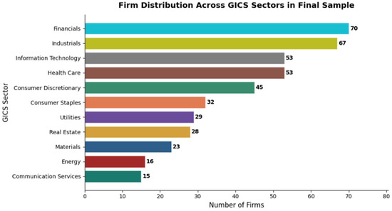
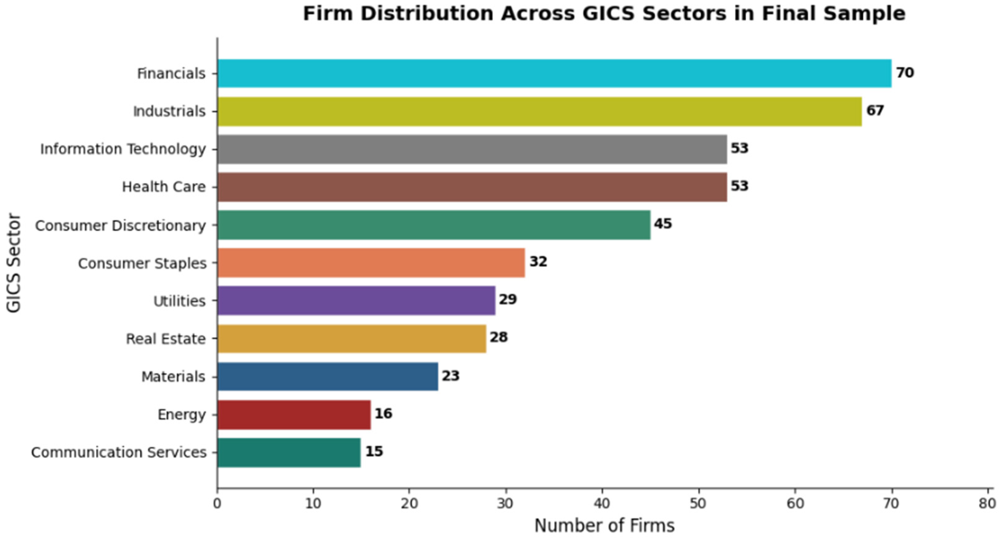
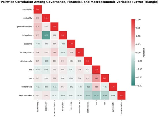
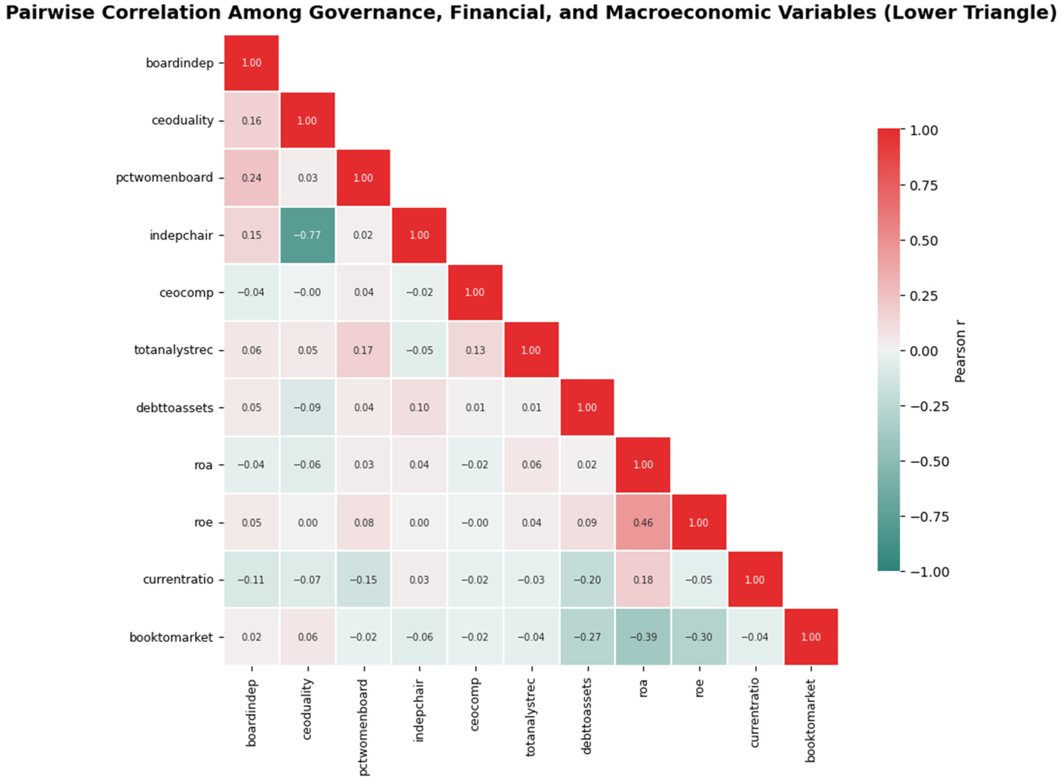
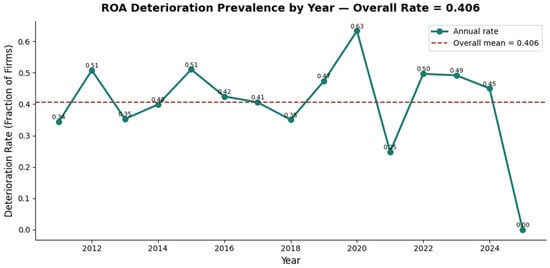
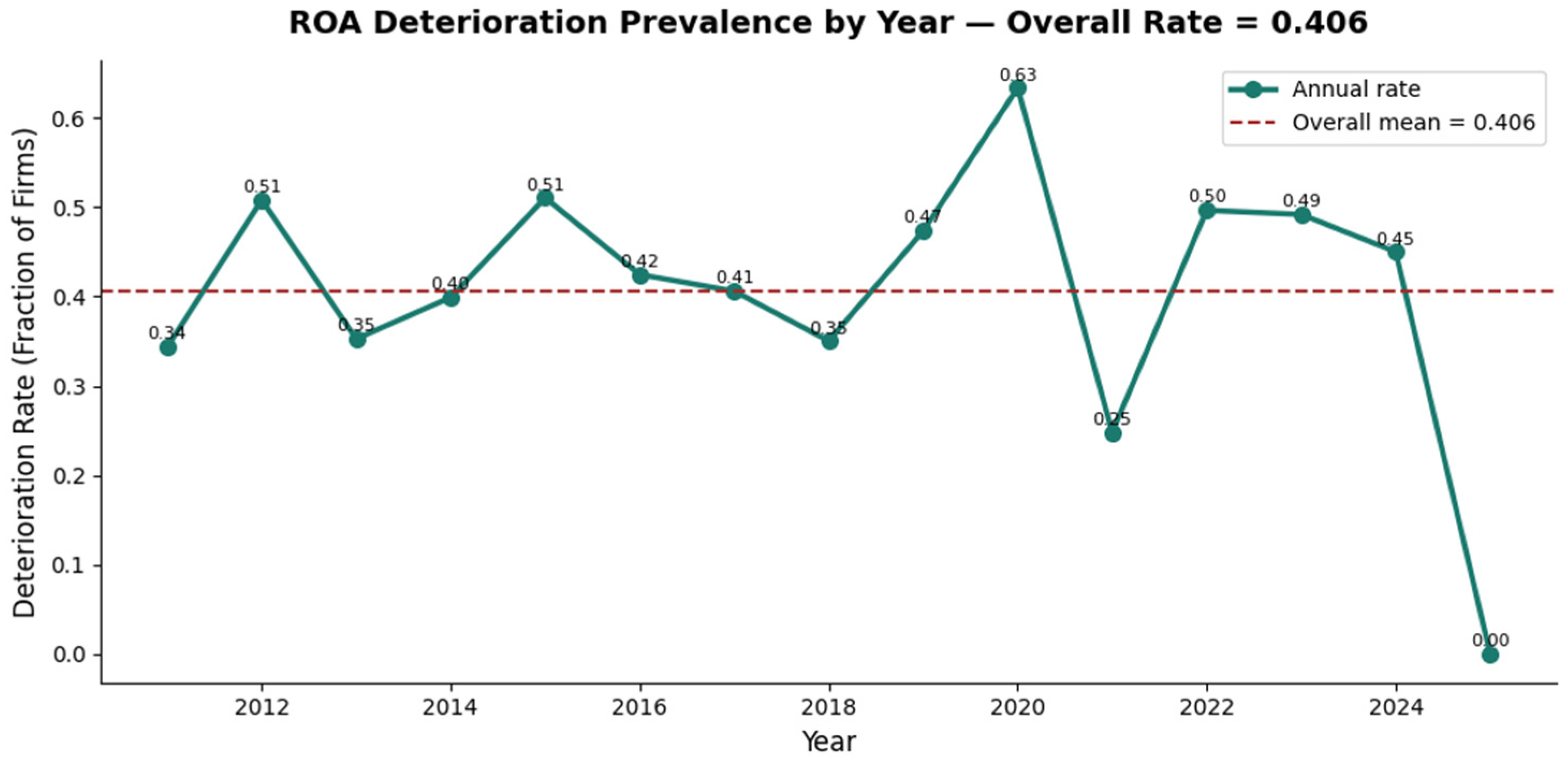
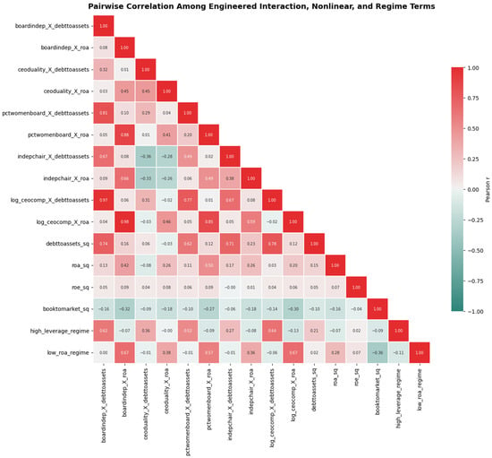
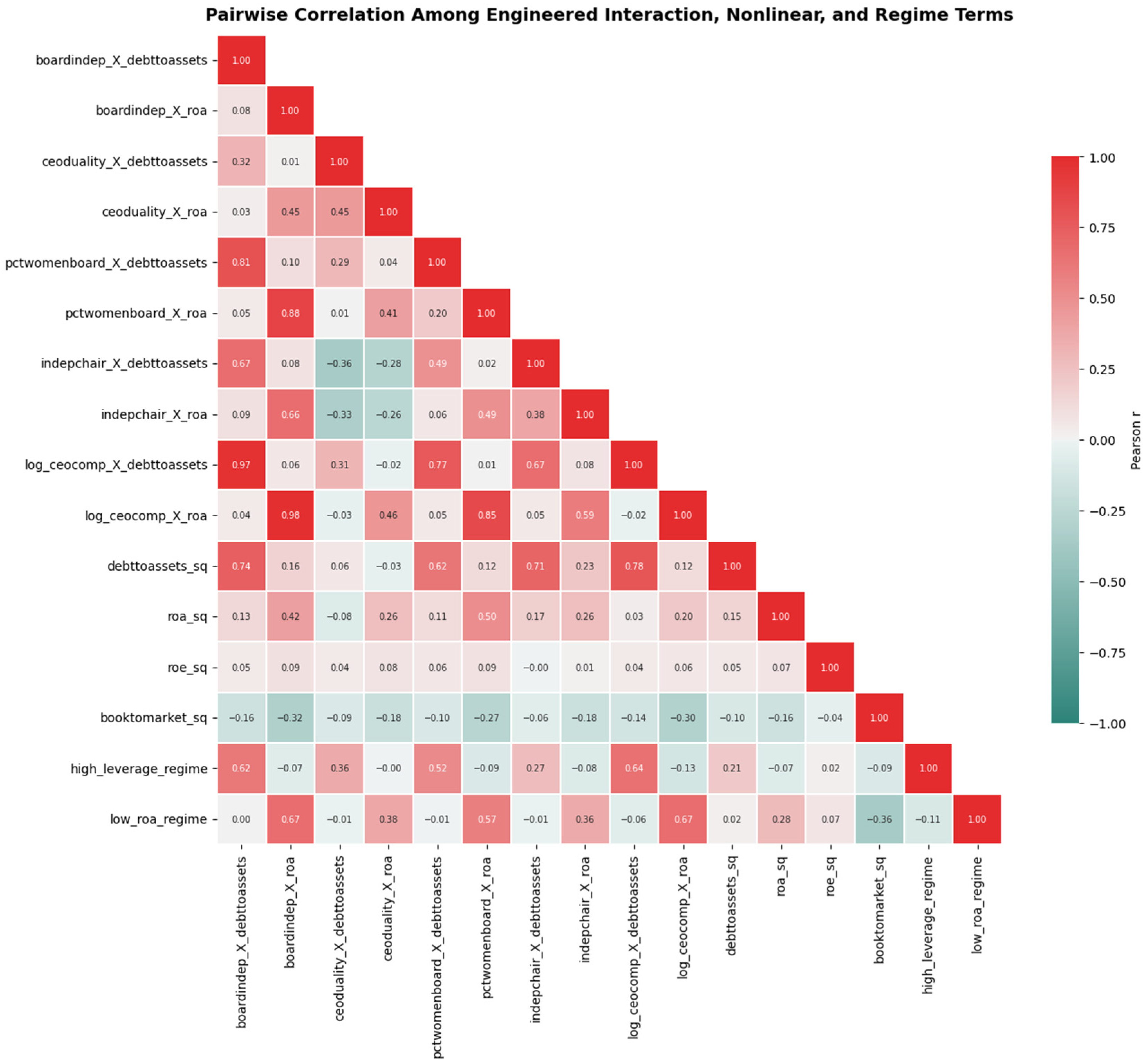
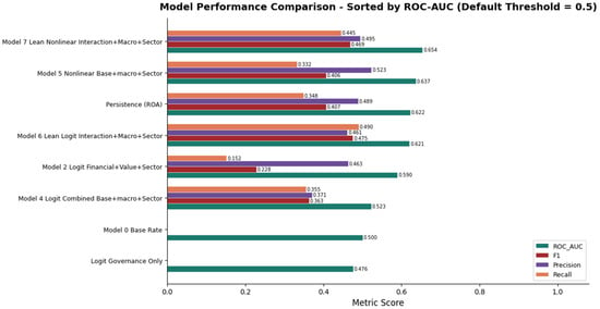
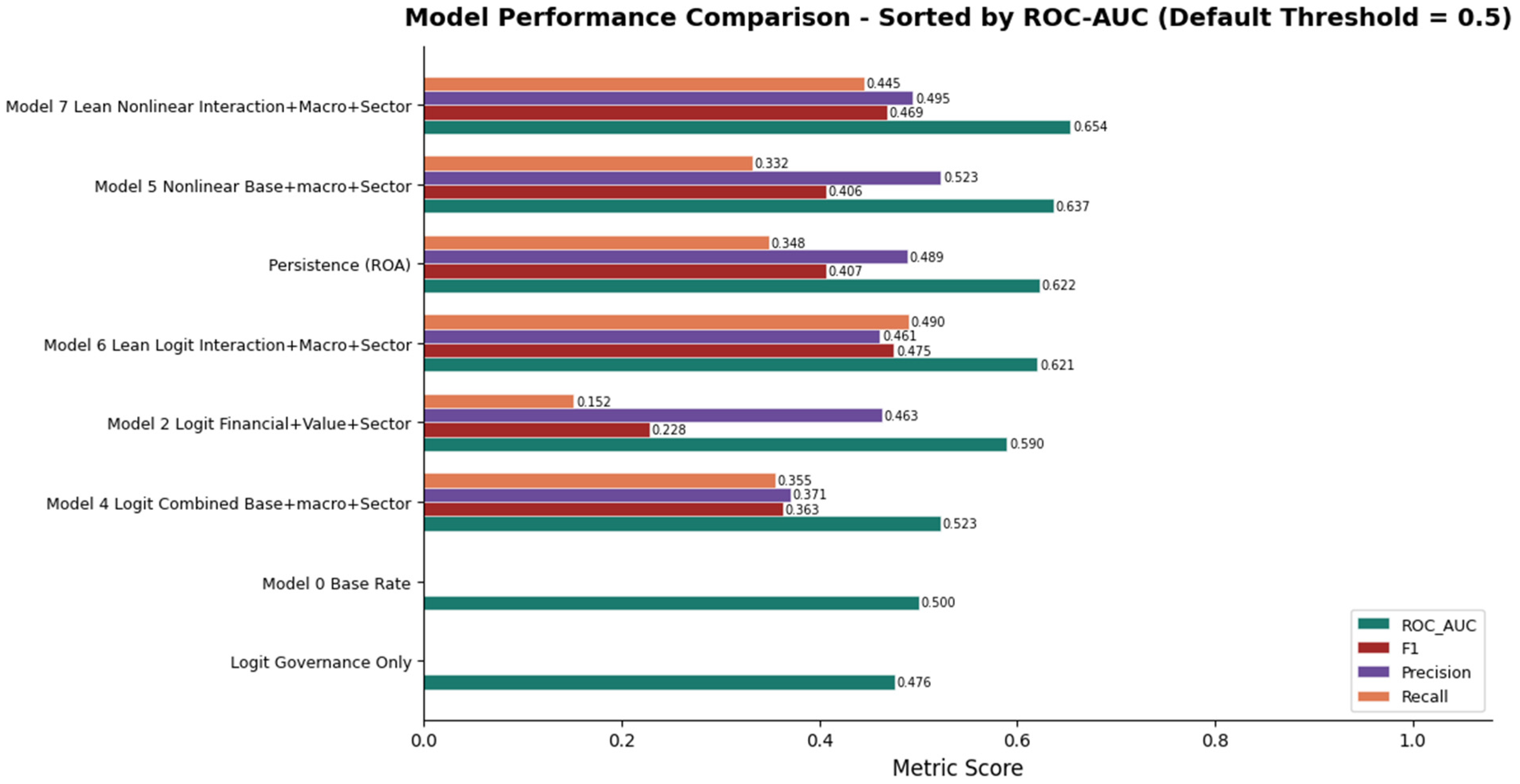
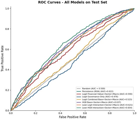
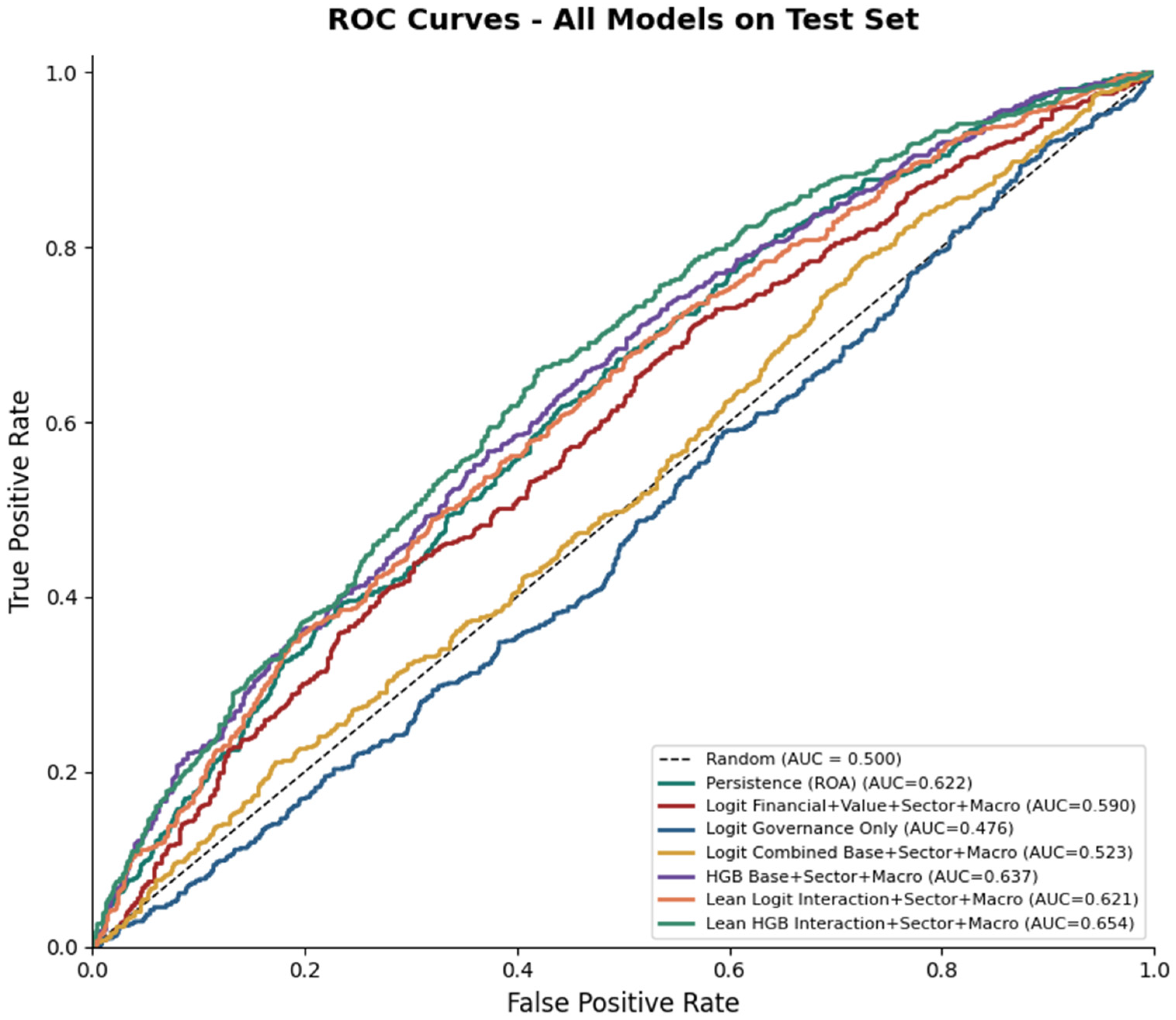
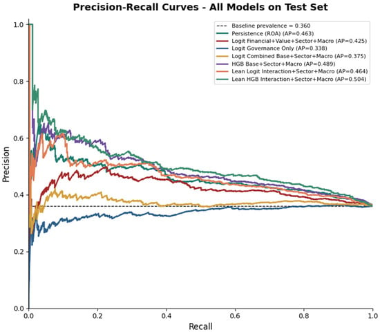
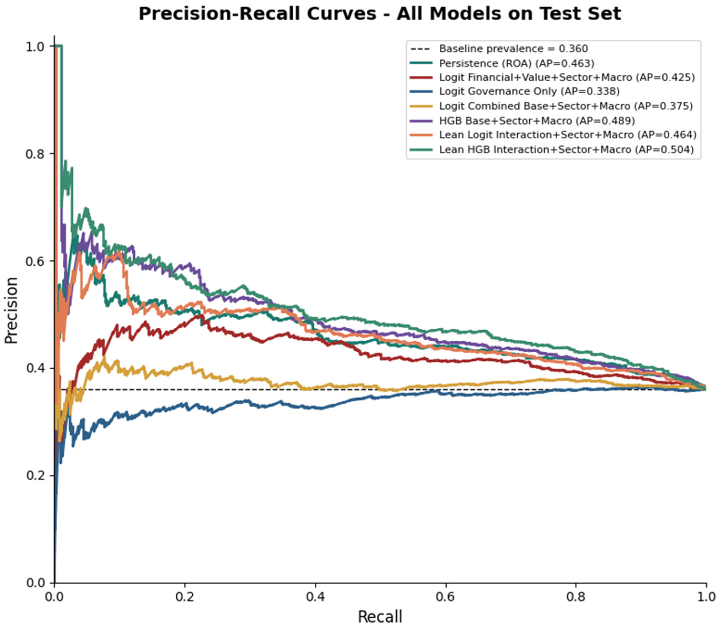
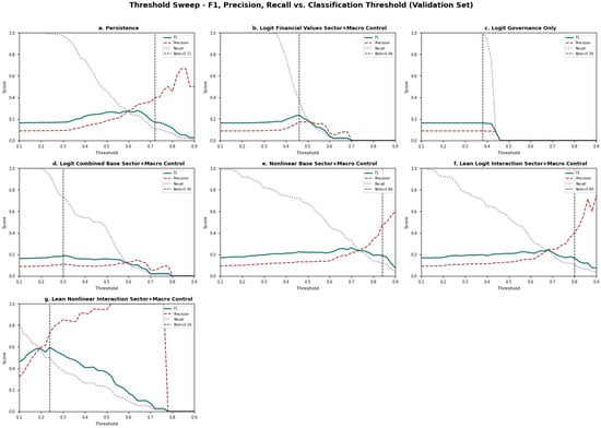
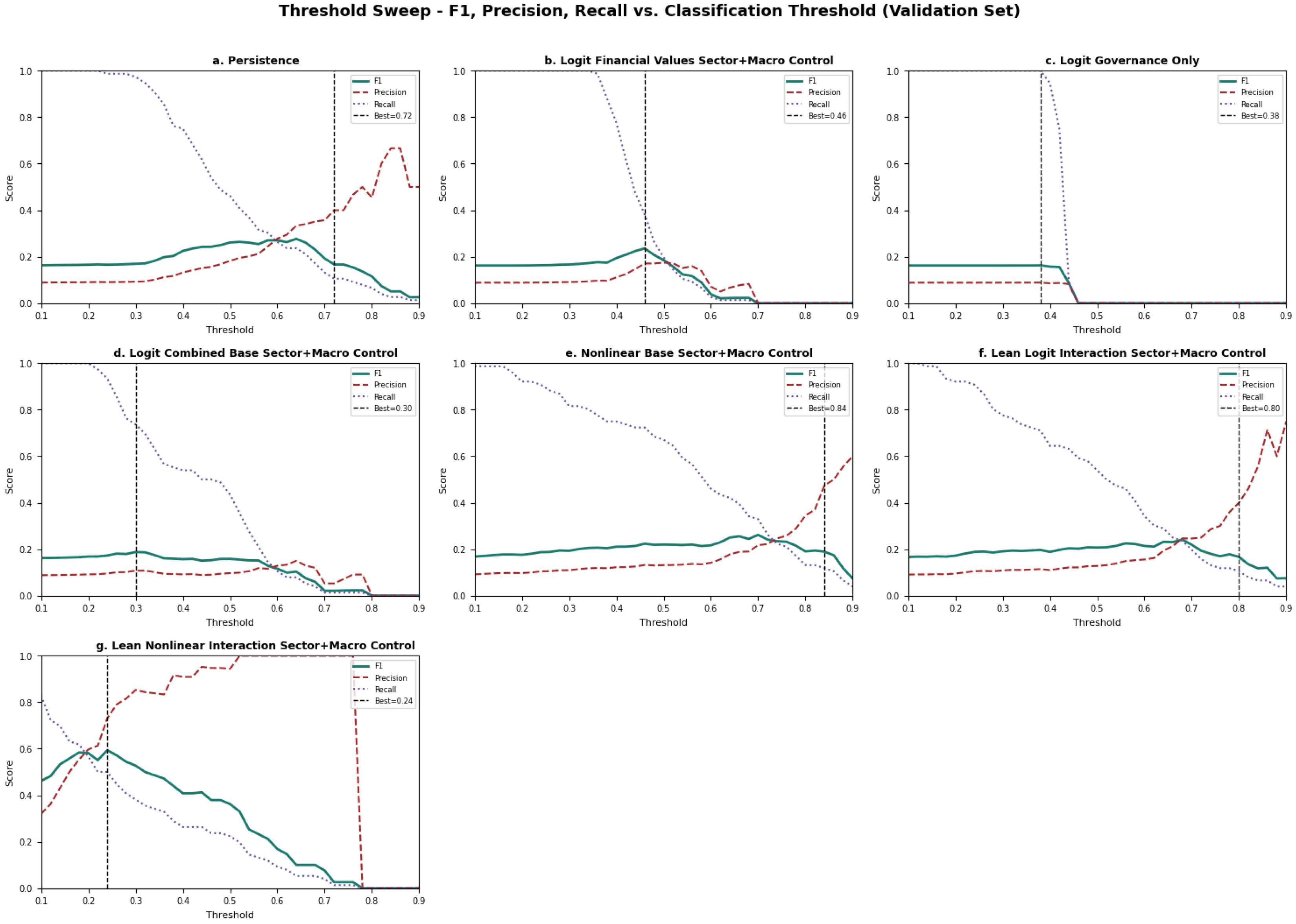
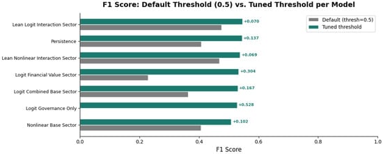
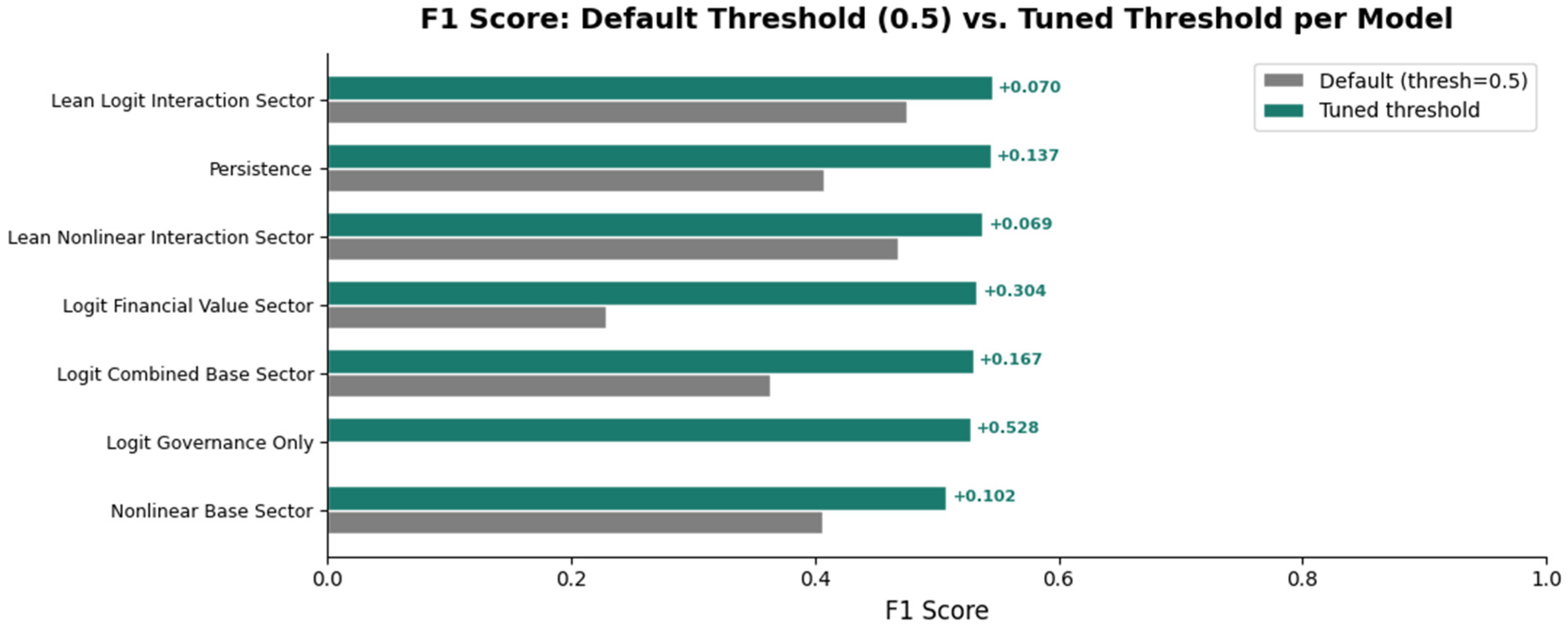
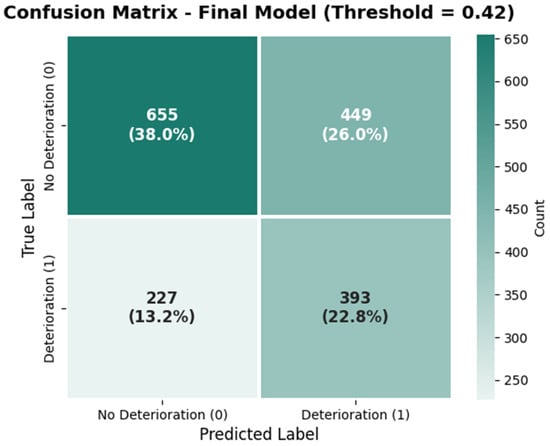
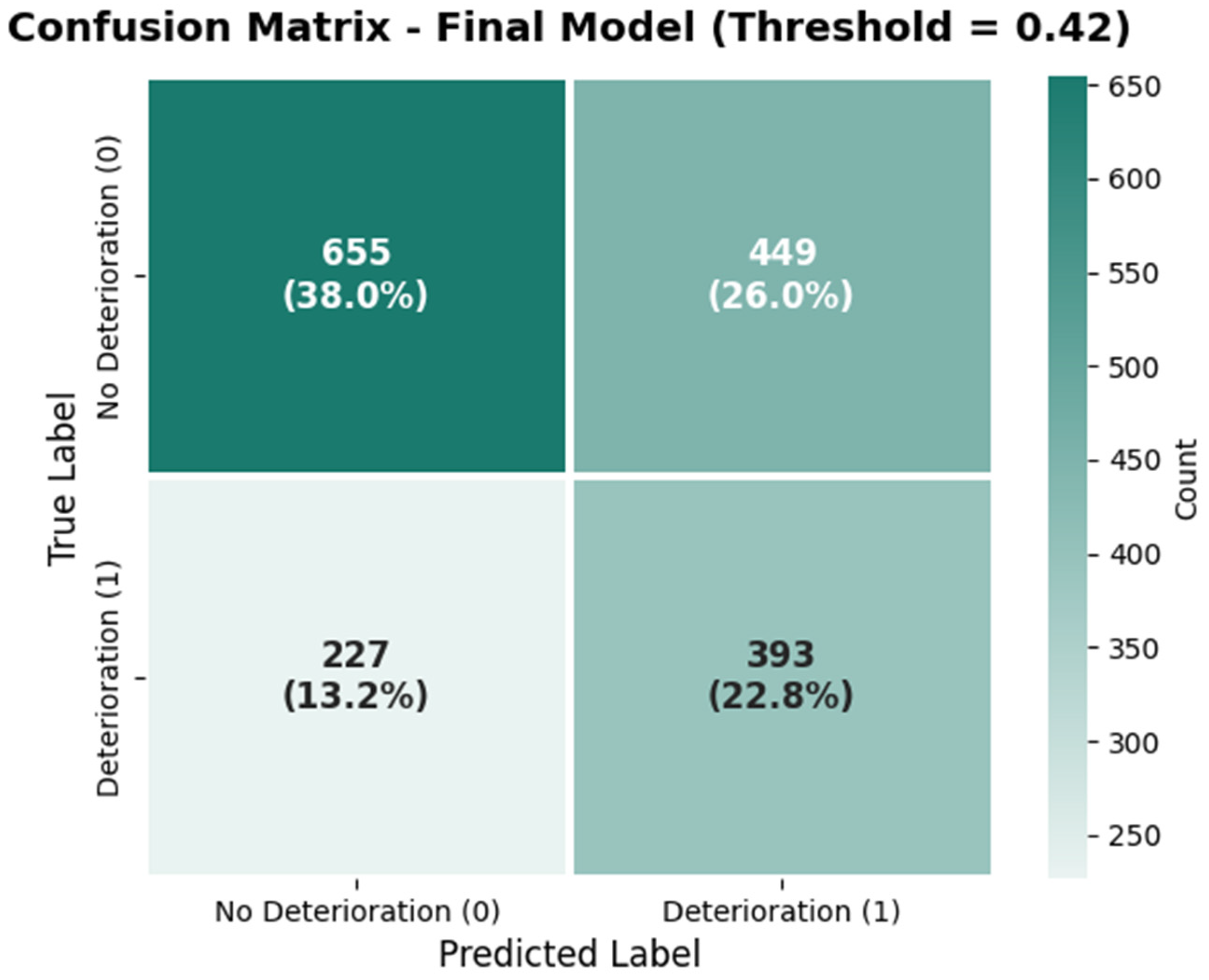
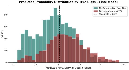
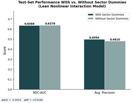
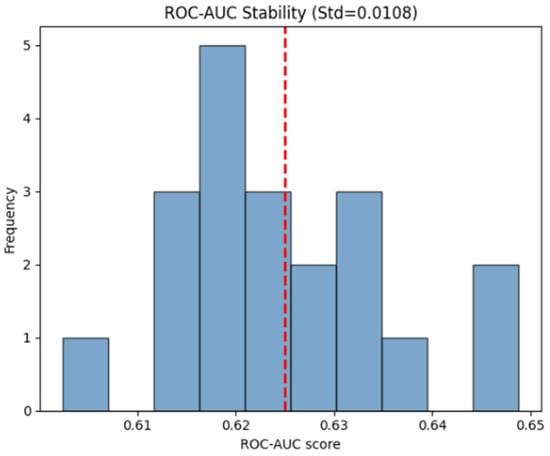
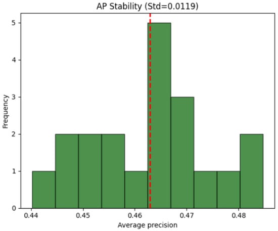
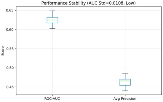
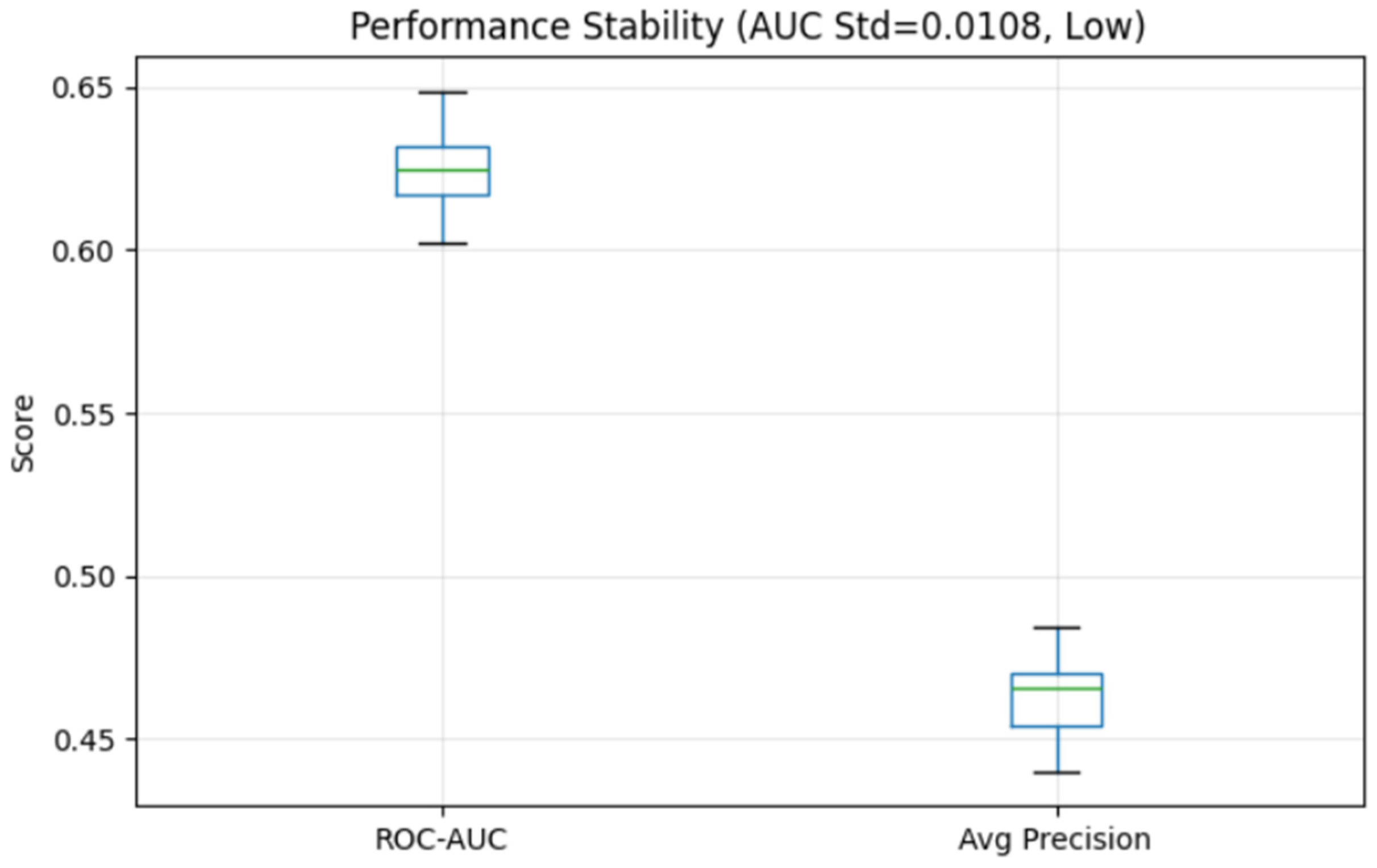
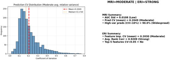
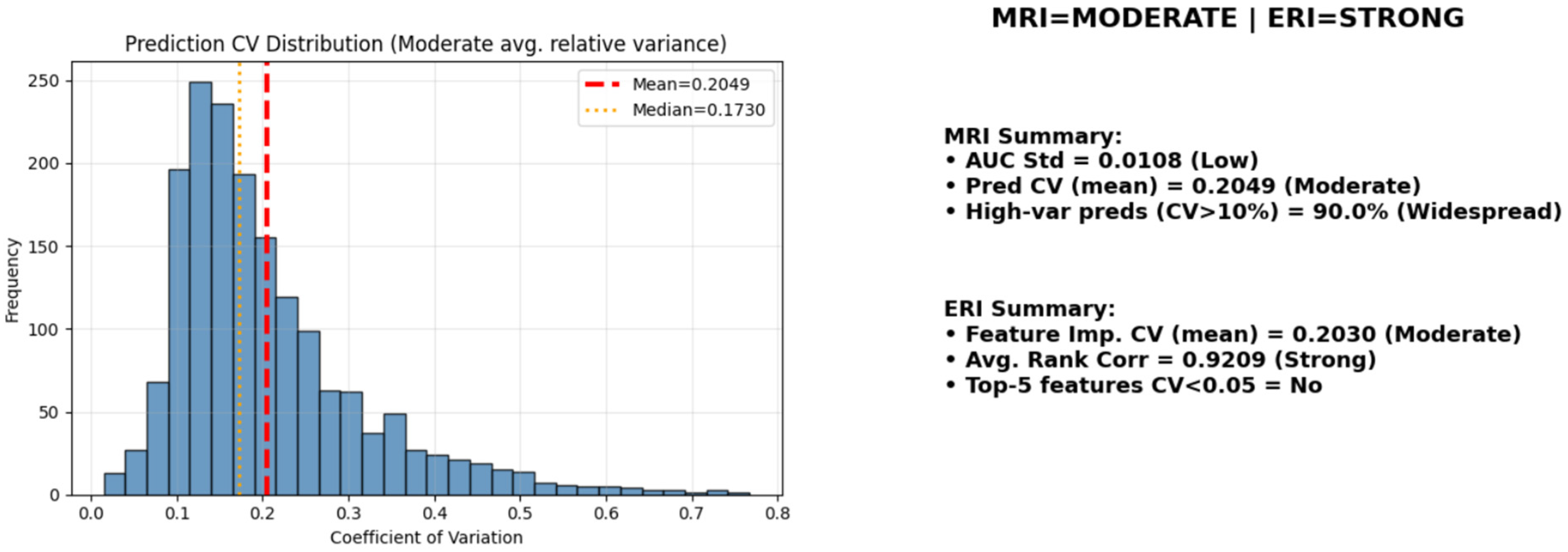
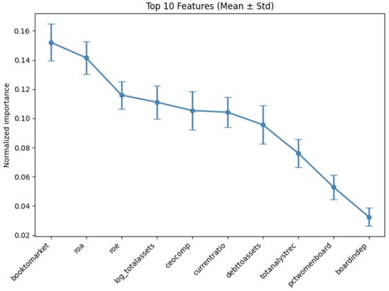
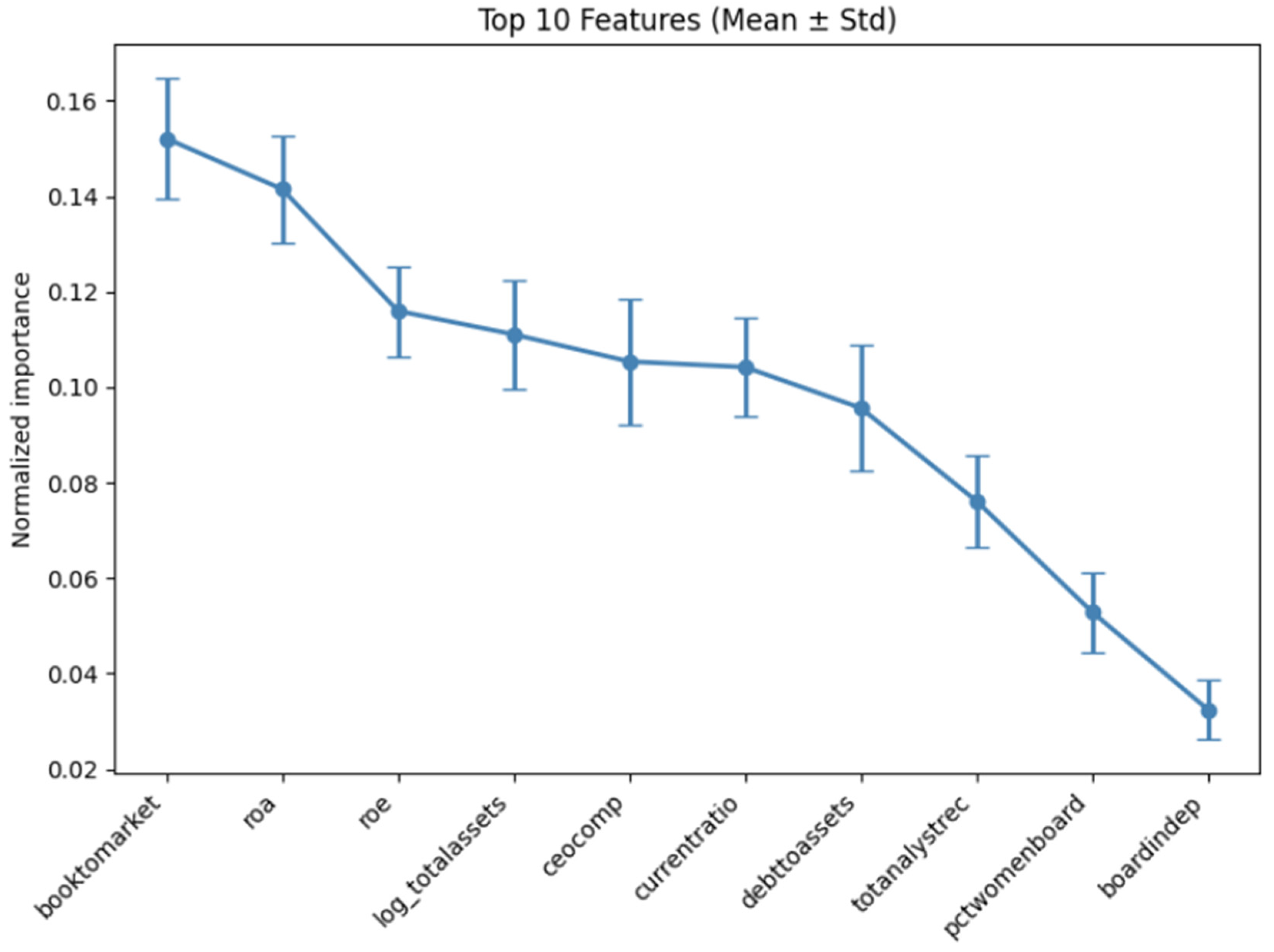
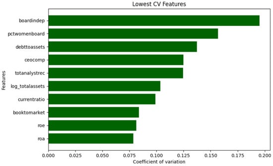
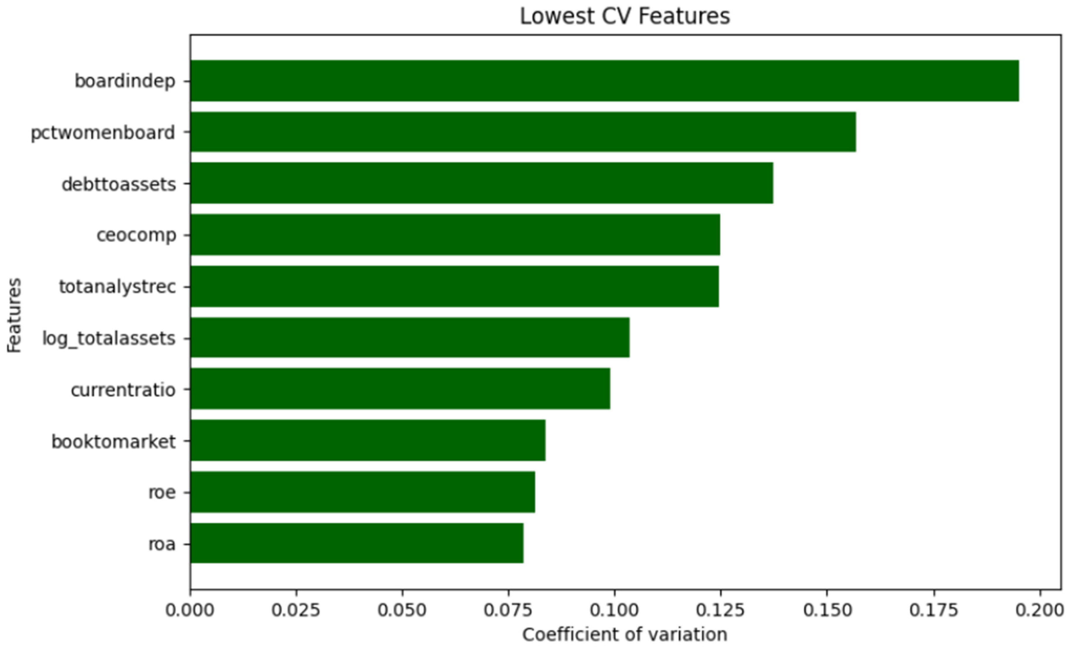
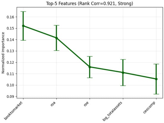
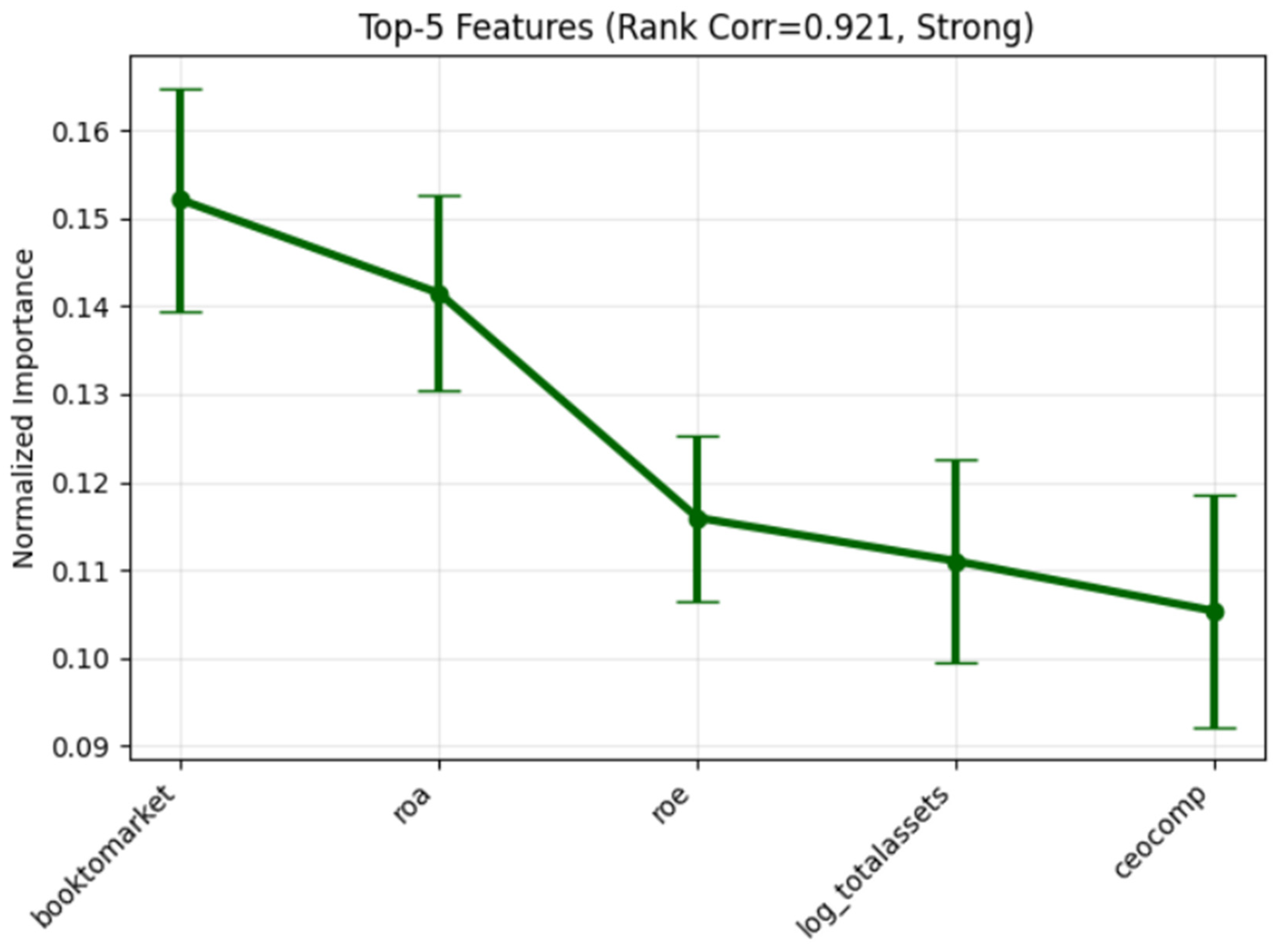
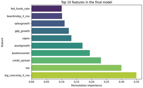
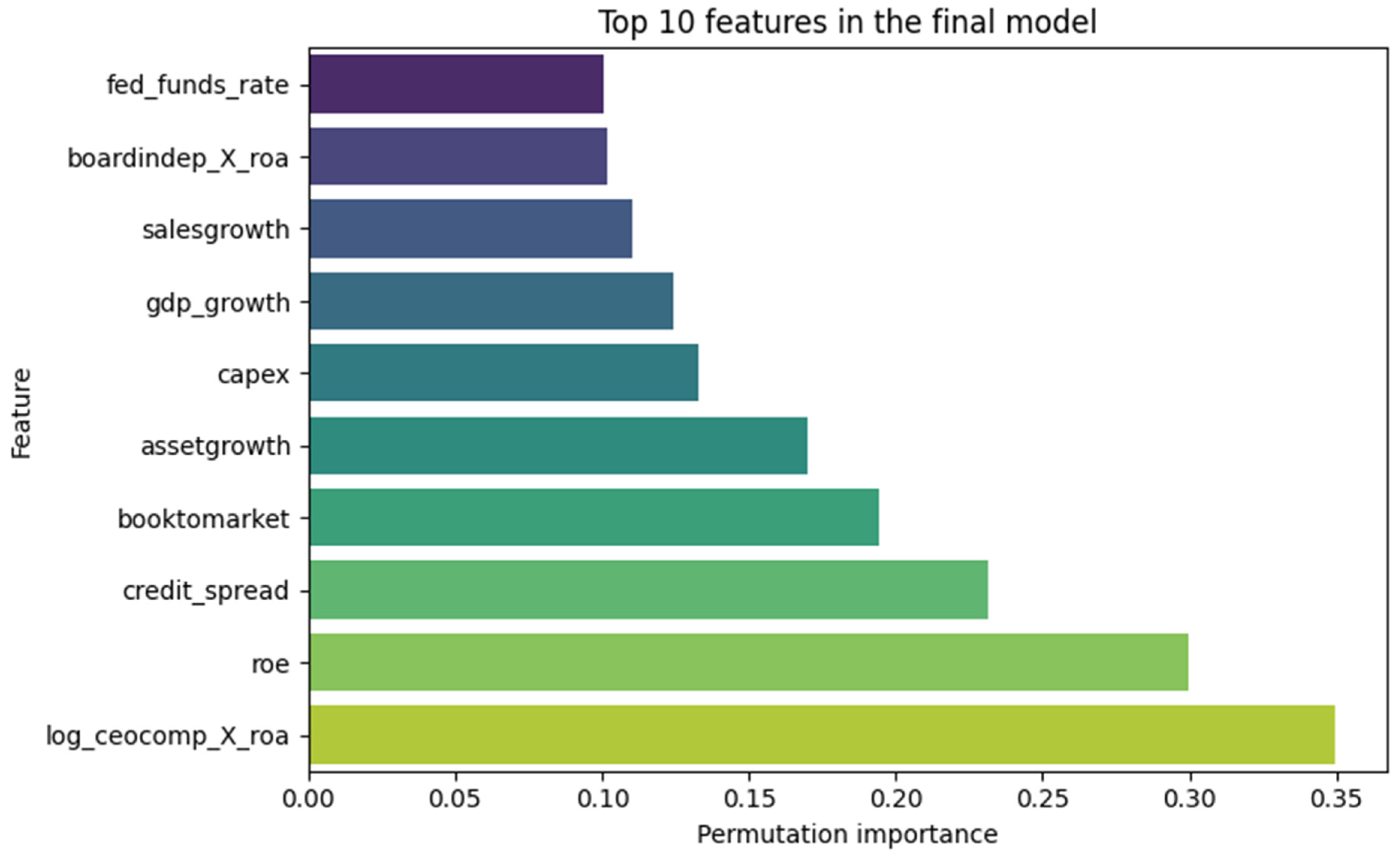
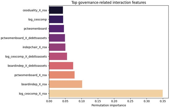
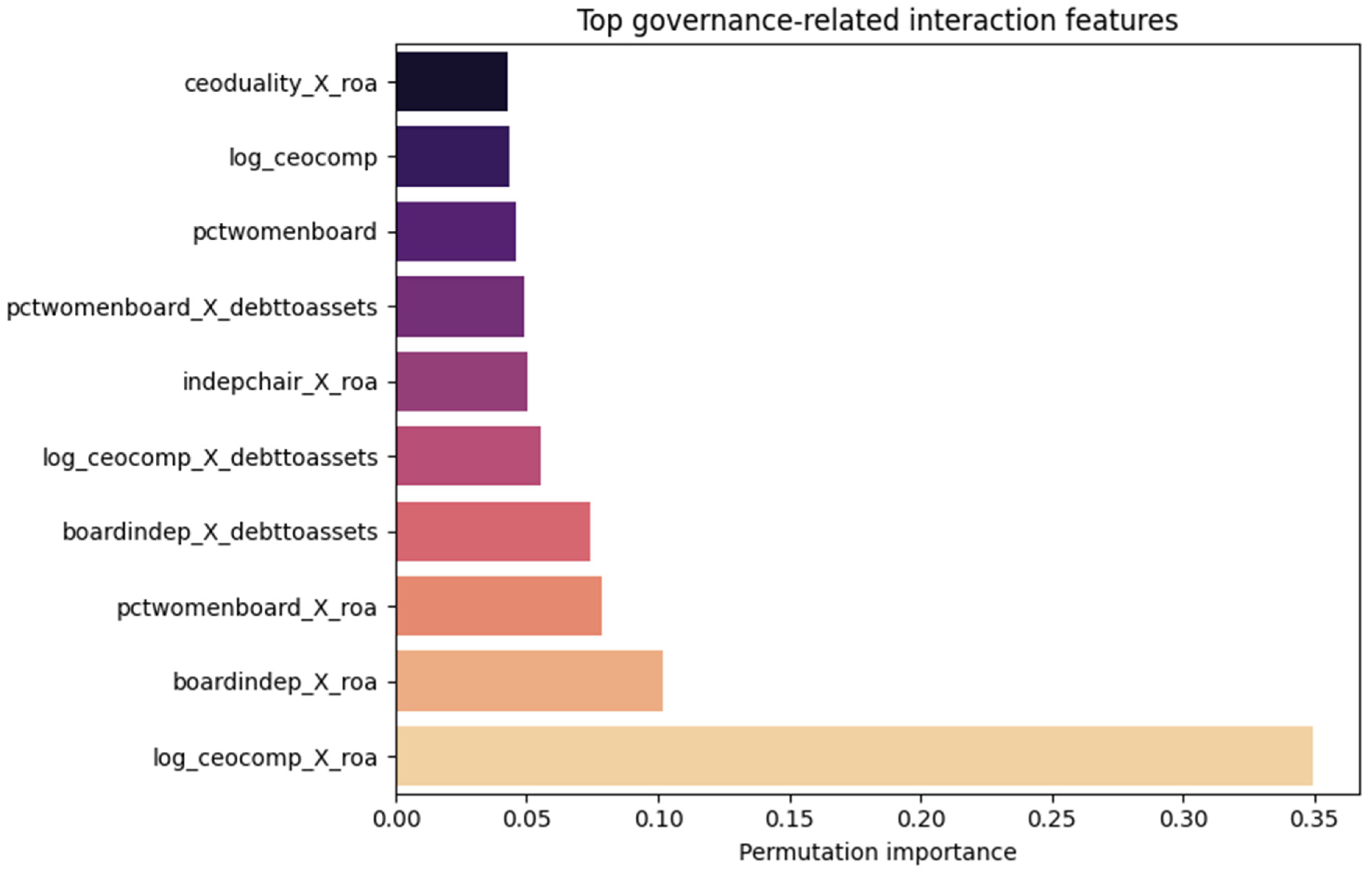
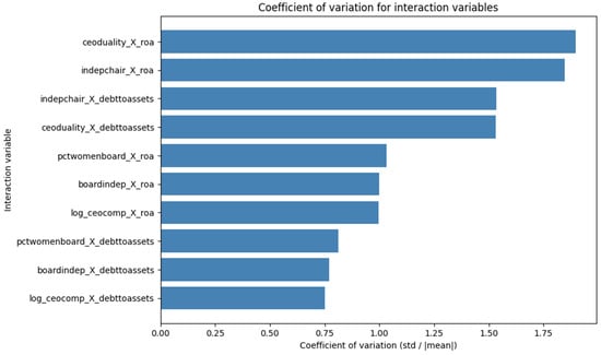
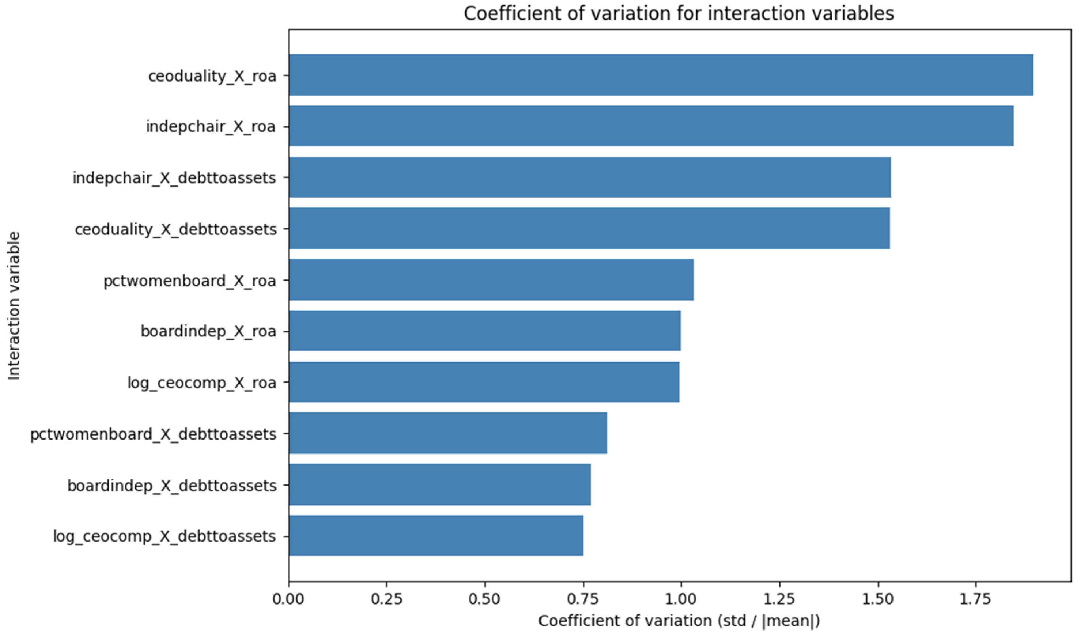
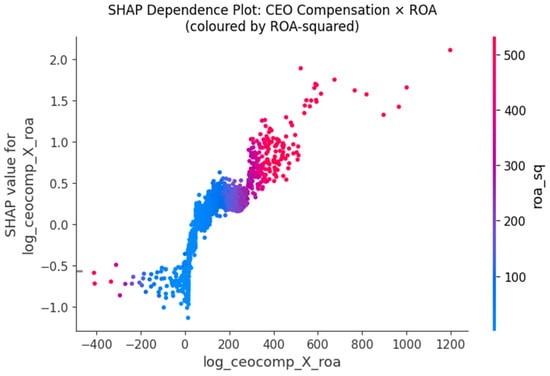
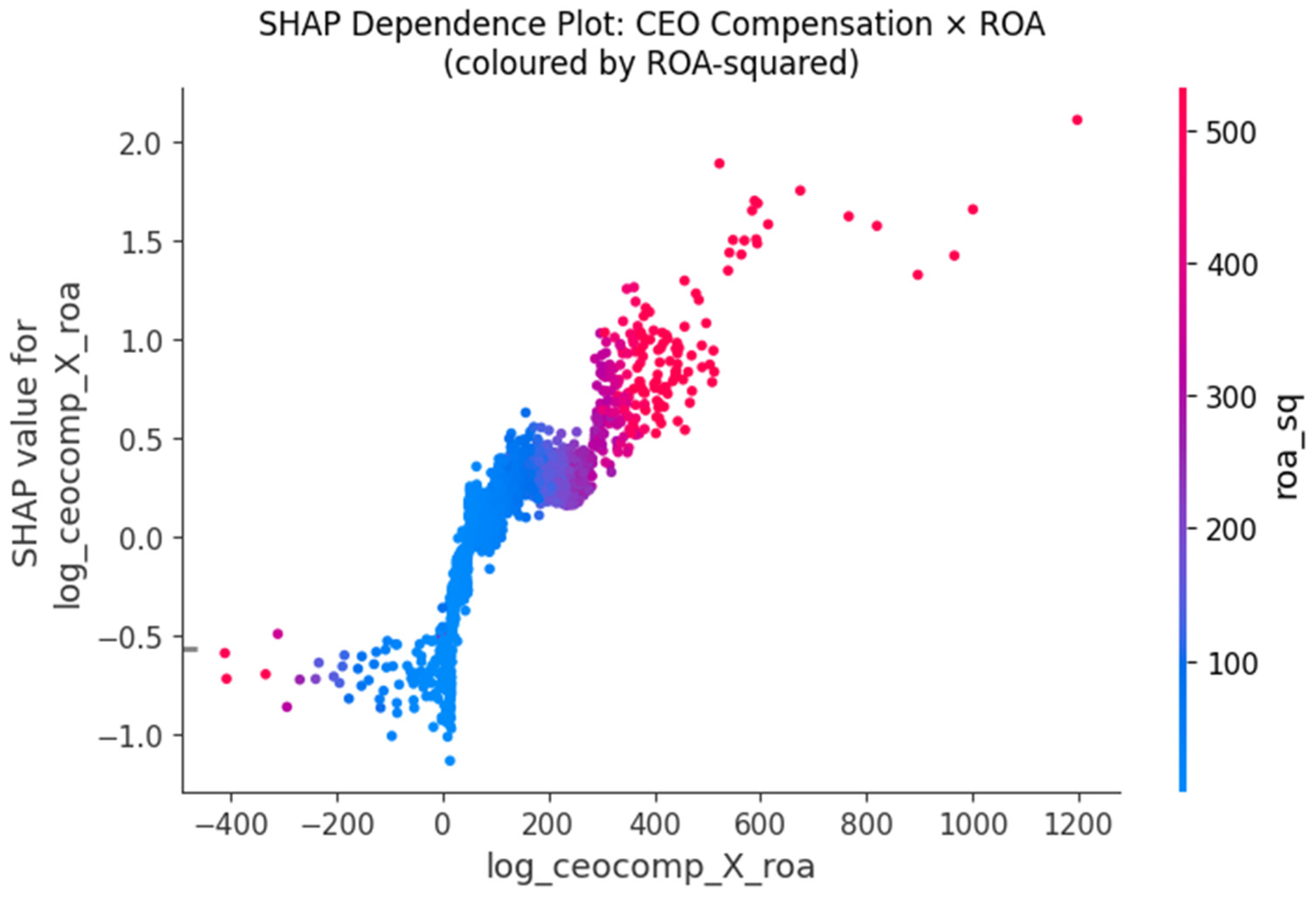
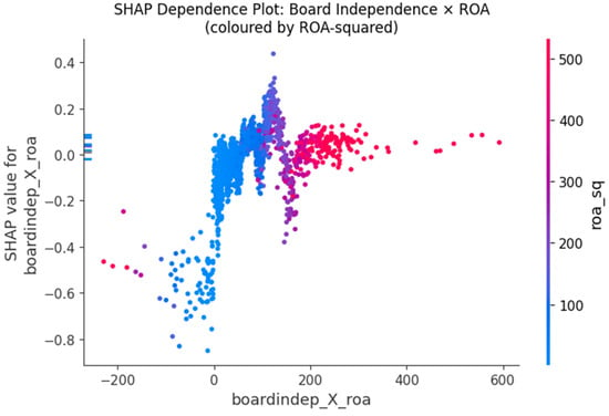
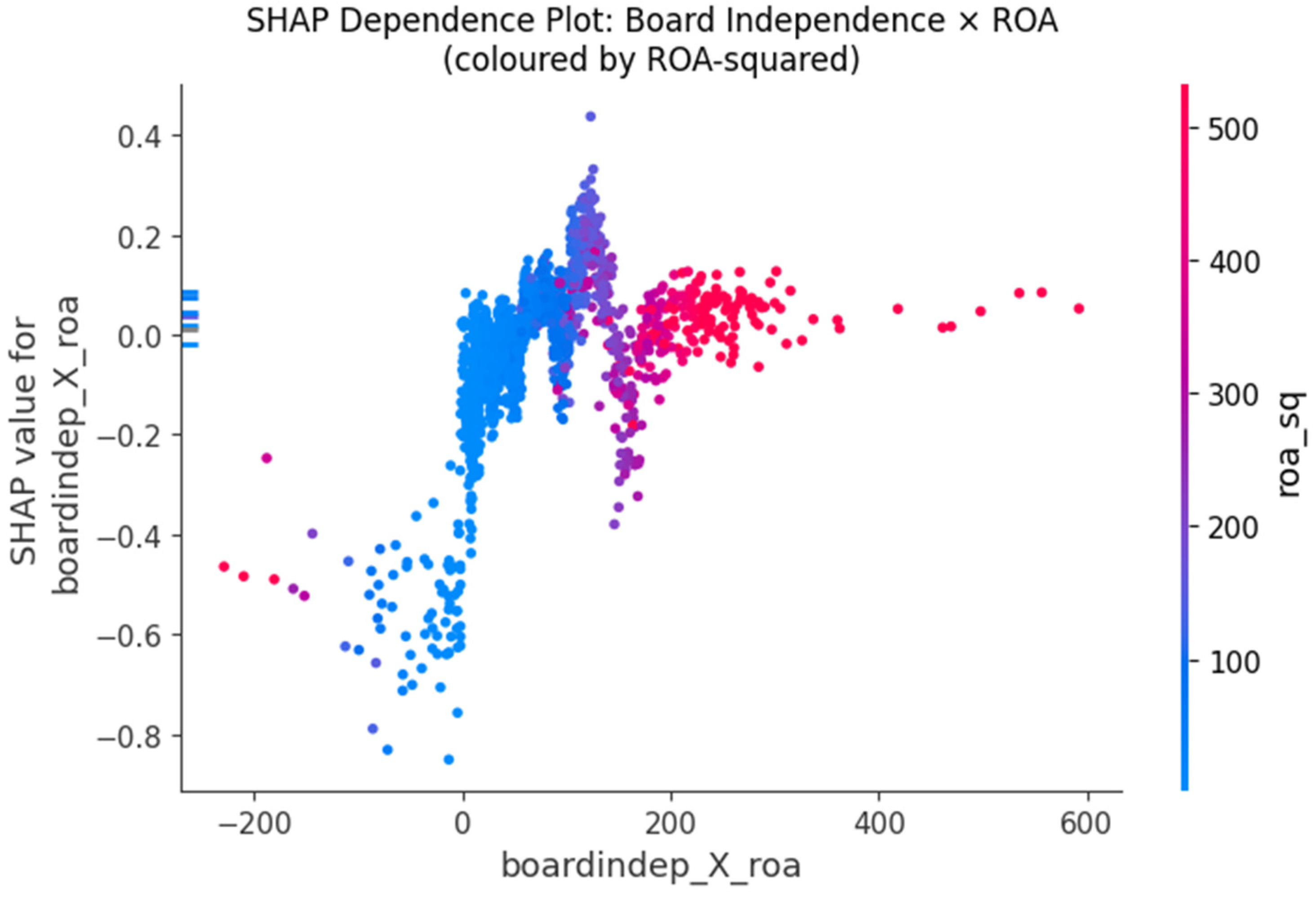
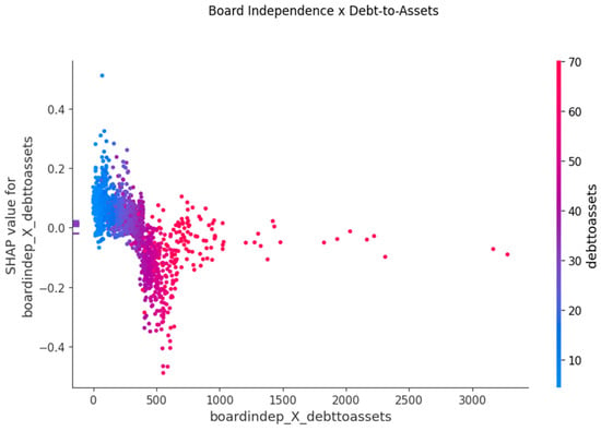
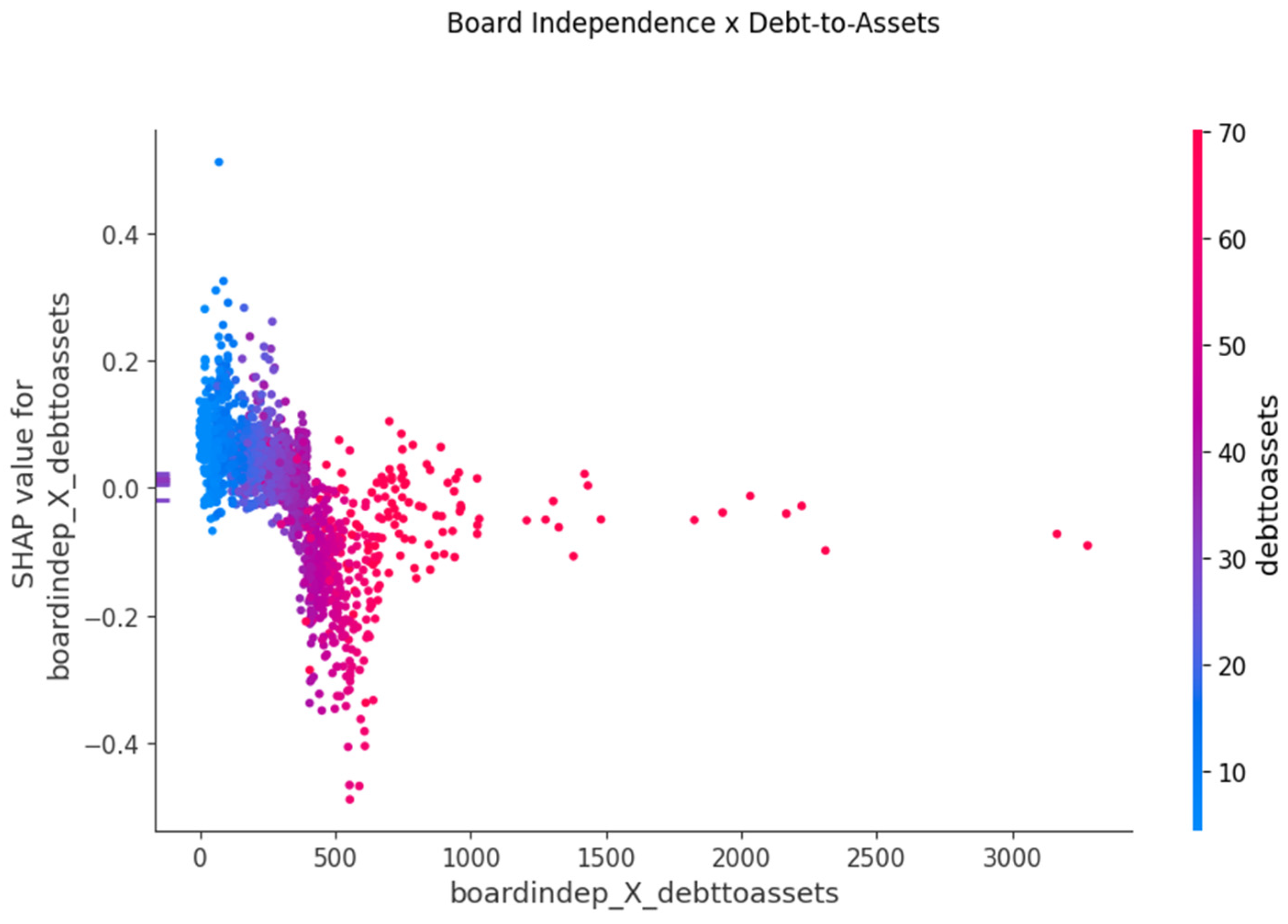
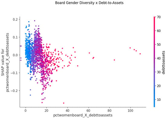
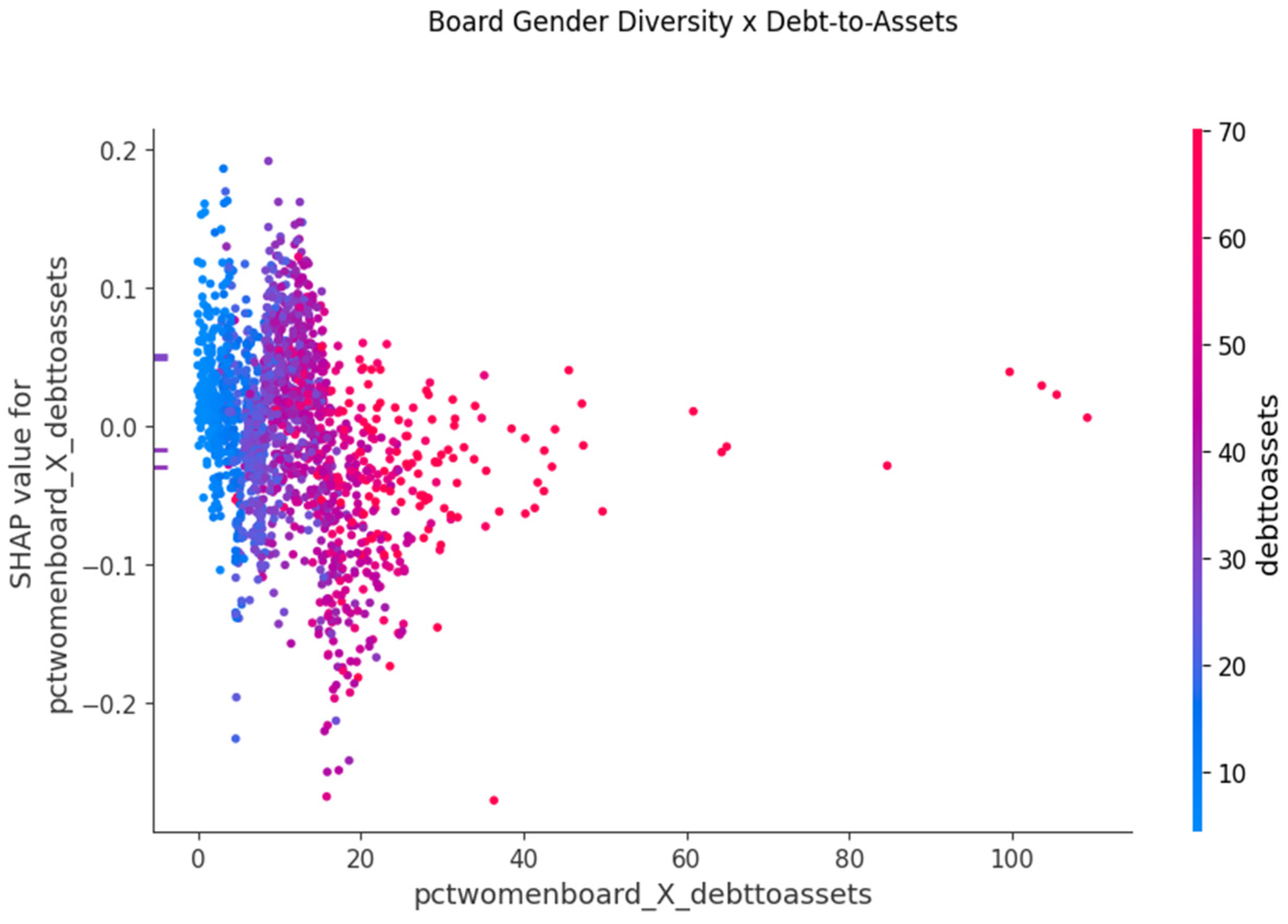
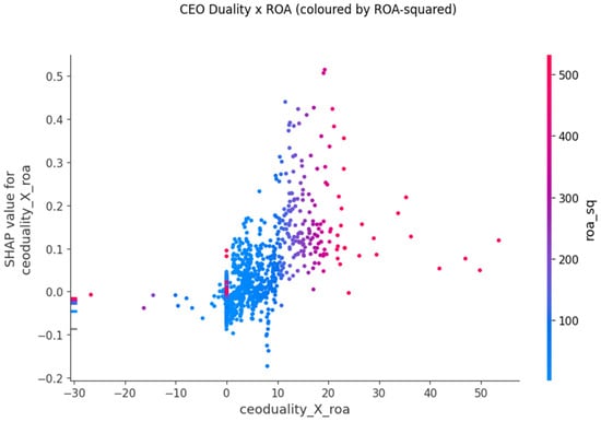
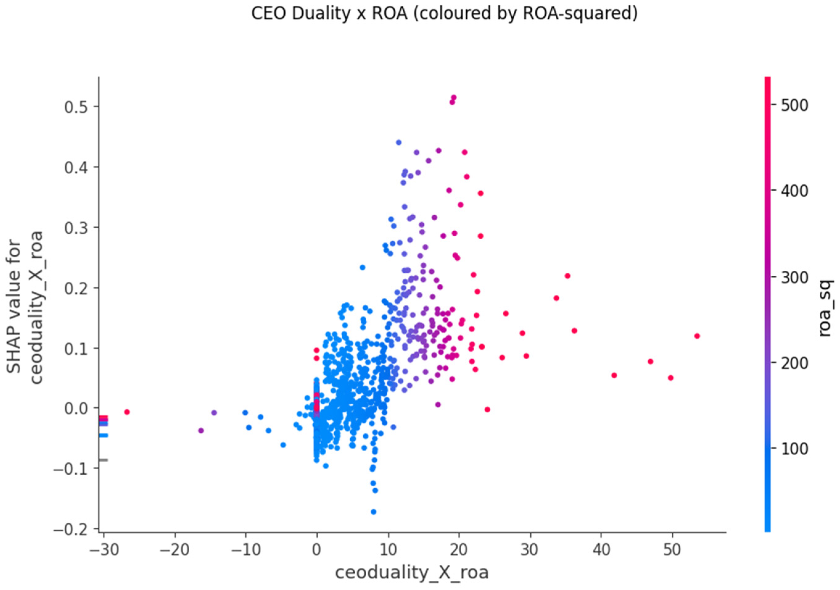
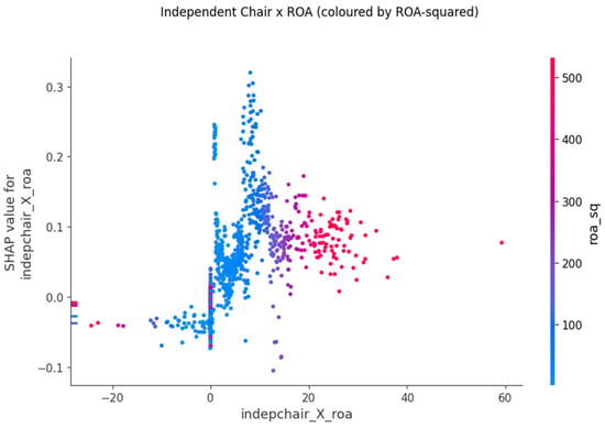
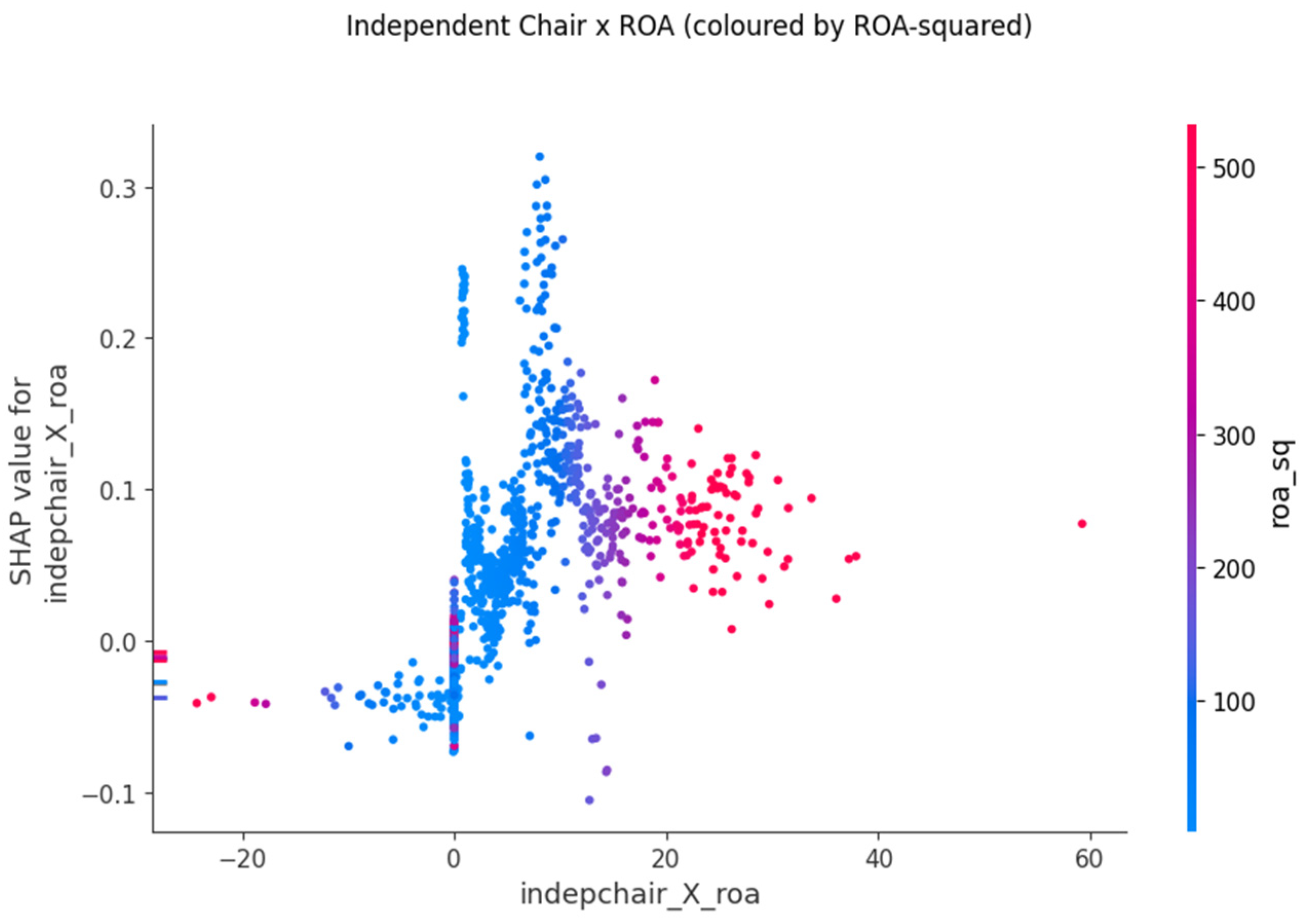
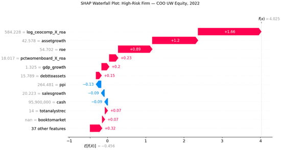
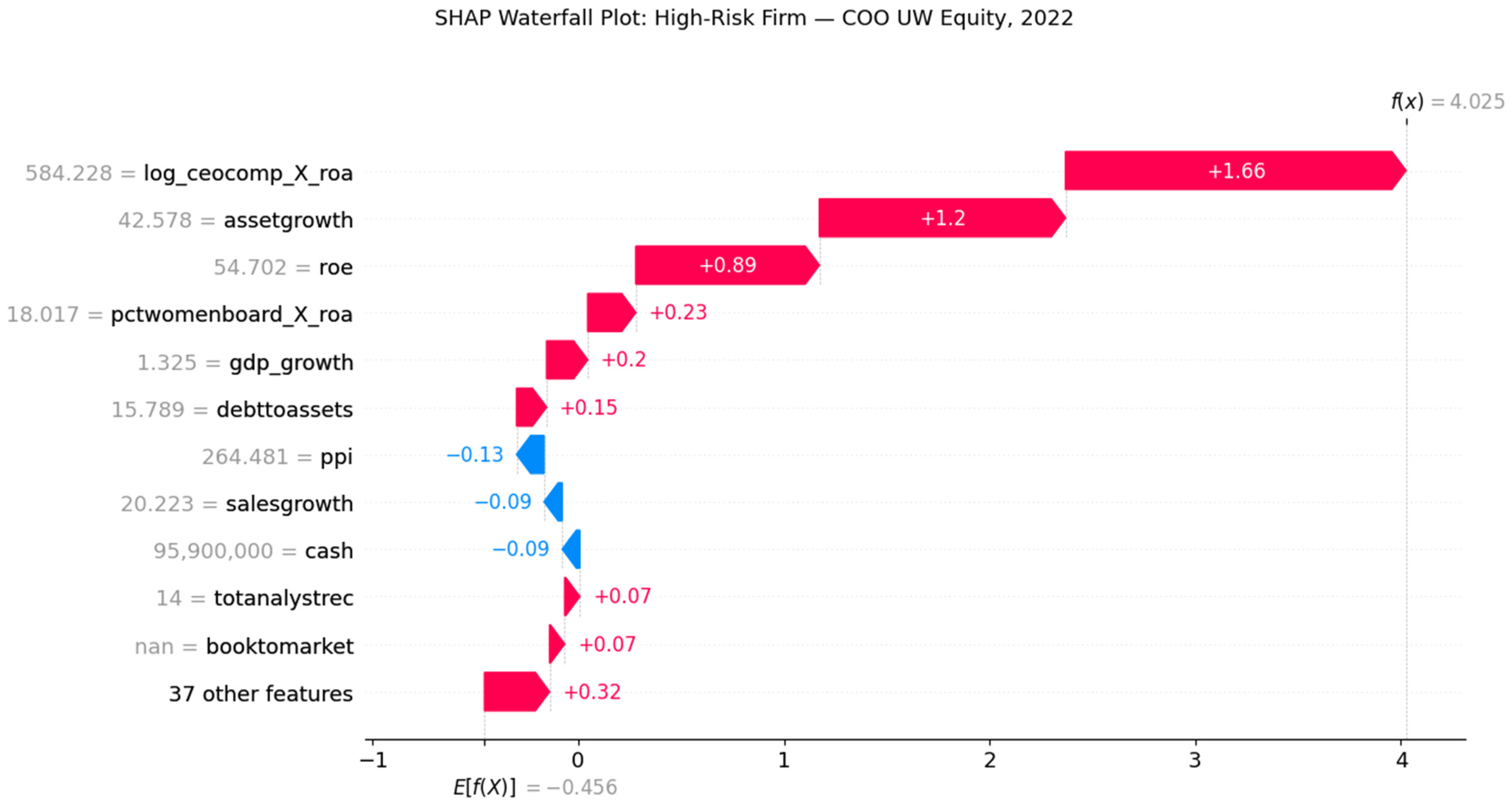
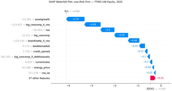
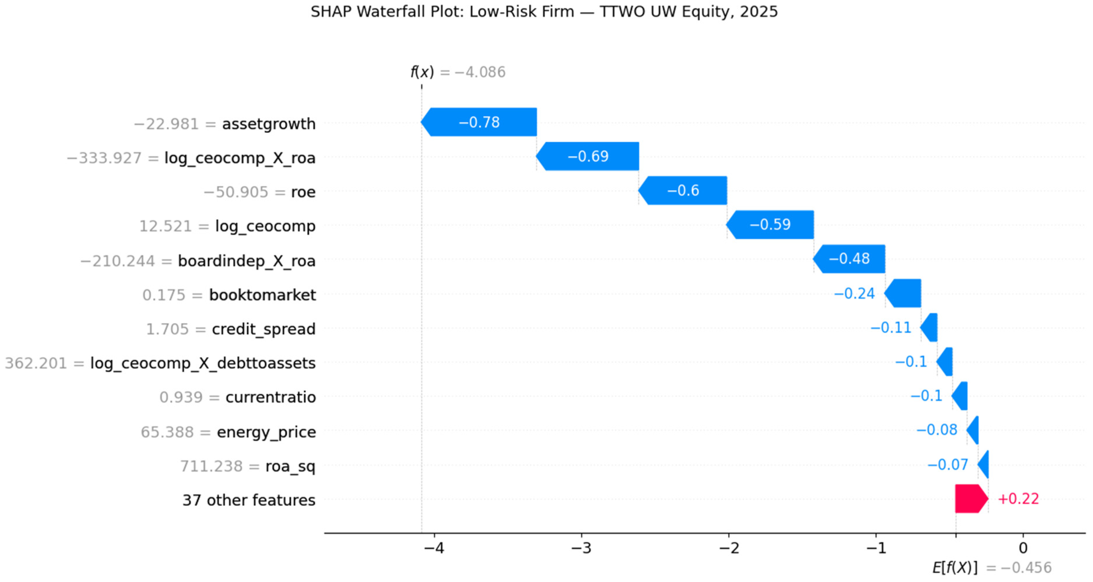
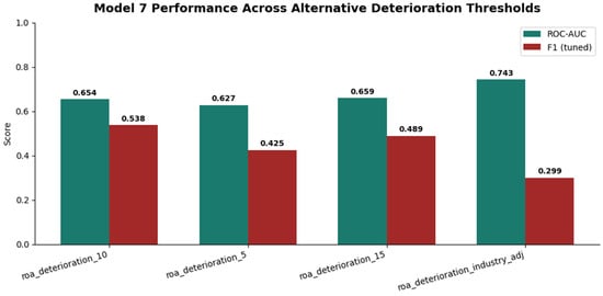
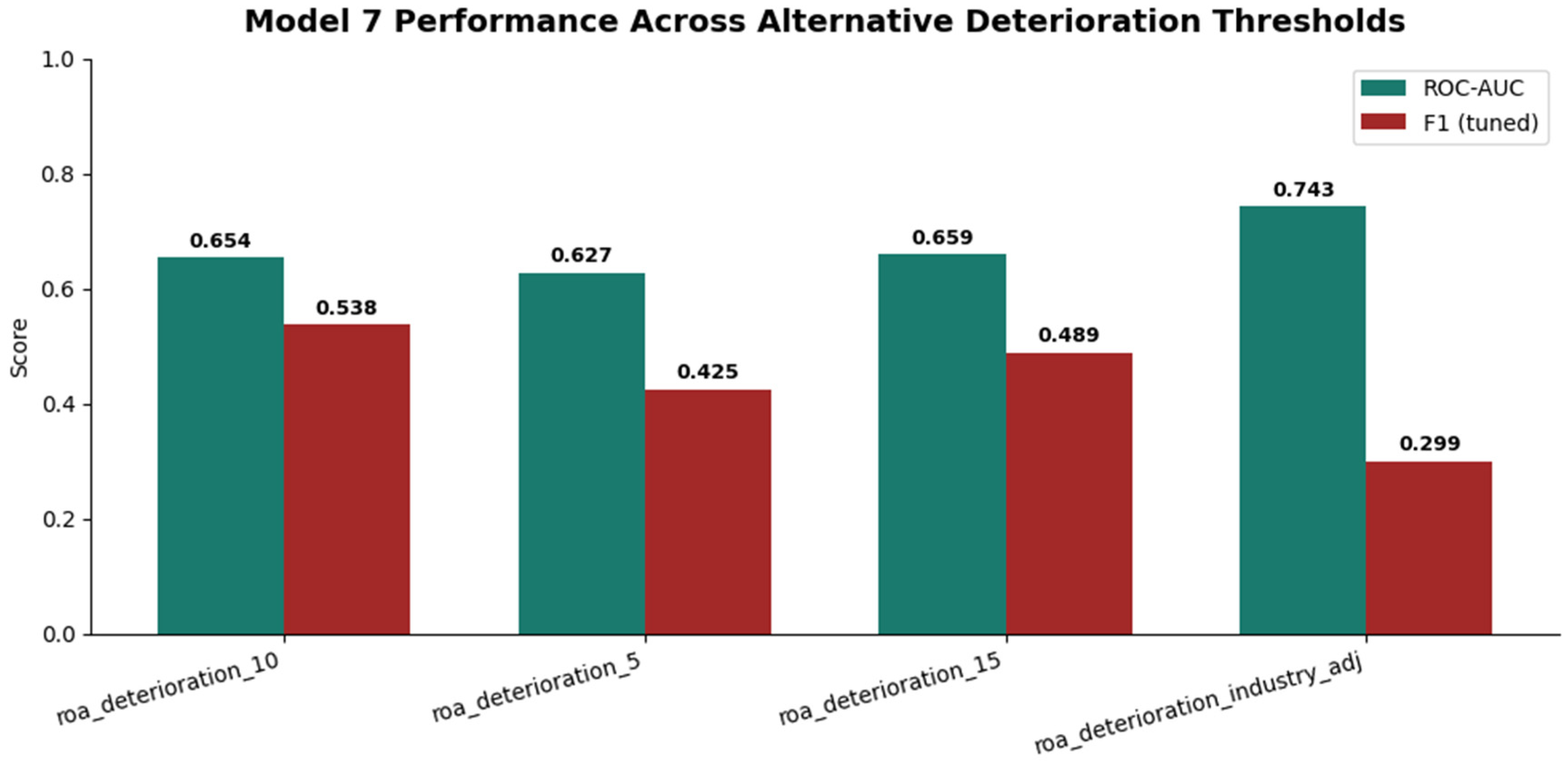

Disclaimer/Publisher’s Note: The statements, opinions and data contained in all publications are solely those of the individual author(s) and contributor(s) and not of MDPI and/or the editor(s). MDPI and/or the editor(s) disclaim responsibility for any injury to people or property resulting from any ideas, methods, instructions or products referred to in the content. |
© 2026 by the authors. Licensee MDPI, Basel, Switzerland. This article is an open access article distributed under the terms and conditions of the Creative Commons Attribution (CC BY) license.