Climate Policy Uncertainty and Corporate Investment: The Real-Estate Concentration Channel

Abstract

Climate policy uncertainty (CPU) suppresses corporate investment broadly, but its effect is not uniform across firms. Using a sample of 60,185 firm-year observations for nonfinancial U.S. firms from 1990 to 2024, this paper shows that industry-adjusted real-estate concentration within the hard-asset base moderates the investment response to CPU. Firms with more real-estate-concentrated tangible assets have lower investment rates on average ($\beta =-0.042$, $t=-18.3$), but under high climate policy uncertainty this negative relation is significantly attenuated in the continuous CPU specification ($t=5.88$). The attenuation is consistent with a structural floor: real-estate-heavy firms already operate in a conservative investment regime, so the additional delay induced by CPU falls disproportionately on firms with more discretionary capital deployment. The financing evidence is mixed rather than uniformly null: leverage interactions are negative (inconsistent with a collateral mechanism), and cash rises modestly under high CPU, but neither pattern absorbs the core investment interaction, pointing to real capital budgeting rather than financial structure as the dominant margin. The result is robust across alternative CPU measures and core specification checks. The evidence is associational rather than causal, but it identifies real-estate concentration as a novel, financial-statement-observable source of firm-level heterogeneity in how climate policy uncertainty transmits to corporate investment, distinct from the aggregate policy shocks, financing constraints, and industry membership emphasized in prior work.

1. Introduction

Climate policy uncertainty (CPU) has become an increasingly important dimension of transition risk for firms making long-lived capital commitments. Unlike general macroeconomic uncertainty, CPU concerns the timing, scope, and distribution of the regulation associated with the transition to a low-carbon economy, including carbon pricing, disclosure rules, and emissions standards, and it remains contested across governments and industries. Gavriilidis (2021) constructs a monthly CPU index from newspaper coverage of climate policy debates and documents a pronounced upward trend since the early 1990s, particularly around major regulatory and international policy episodes, and Ren et al. (2022) link this measure to lower firm-level total factor productivity in China through reduced R&D and free-cash-flow channels, evidence that CPU has real rather than purely financial consequences. The financial relevance of climate-related policy risk is now well established in asset pricing, derivatives markets, and corporate finance (Bolton and Kacperczyk 2021; Ilhan et al. 2021; Sautner et al. 2023), and recent work formalizes climate change itself as a source of model uncertainty and ambiguity with first-order asset-pricing consequences (Barnett et al. 2020). A closely related transition-risk literature studies stranded assets, namely the possibility that regulatory or technological change strands physical capital before the end of its useful life, and Daumas (2024) surveys the theoretical and applied evidence linking this risk to financial stability; the mechanism studied in the present paper is a milder, continuous version of the same underlying concern, in which uncertainty about future policy attenuates investment in hard-to-redeploy assets rather than stranding them outright. More recent evidence extends this relevance from valuation to firm-level real and adaptive behavior (Li et al. 2024; Pankratz and Schiller 2024), but much less is known about which firms adjust their investment behavior most strongly when climate policy uncertainty rises; the present paper studies U.S. firms and focuses on investment as the outcome and real-estate concentration as the heterogeneity margin, a combination not examined in that literature.

This question is naturally framed by the broader investment-under-uncertainty literature. When the regulatory environment is unclear, firms facing irreversible capital commitments have an incentive to delay investment until uncertainty is resolved; profitability that depends on an unsettled policy path makes waiting more valuable than committing capital immediately. This logic is central to the real-options framework (Bernanke 1983; Dixit and Pindyck 1994) and has been documented empirically in both aggregate and firm-level settings. Bloom (2009) shows that uncertainty shocks are associated with sharp contractions in investment and hiring, while Baker et al. (2016), Gulen and Ion (2016), and Julio and Yook (2012) find that elevated policy uncertainty is linked to lower corporate investment. More recent climate-specific evidence points the same way: financially constrained firms facing a discrete climate-policy shock reallocate emissions and output across plants rather than adjusting investment uniformly (Bartram et al. 2022), suggesting that policy and transition shocks have real, not merely valuation, effects on corporate behavior. Together, this literature suggests that uncertainty is especially consequential when firms face costly or difficult-to-reverse capital commitments, and this paper adopts the real-options, investment-under-uncertainty framework as its guiding theoretical lens throughout: irreversible capital commitments create option value in waiting, so cross-sectional variation in the cost of reversing a given commitment should generate cross-sectional variation in the strength of the uncertainty–investment relation.

A central open question, however, is why the investment response to climate-related uncertainty should differ across otherwise similar firms. One plausible source of heterogeneity is the composition of the hard-asset base: firms with less redeployable or more asset-specific capital respond differently to uncertainty and face different adjustment margins in investment and financing (Kermani and Ma 2023; Kim and Kung 2017). Owned real estate is a particularly useful setting for this question. Buildings and land are costly to transact, slow to repurpose, and typically embedded in long-lived, location-specific operating decisions, making them a relatively rigid and more committed form of physical capital than machinery or equipment. This distinction is separate from the collateral role of real estate emphasized by Chaney et al. (2012), Kiyotaki and Moore (1997), and Rampini and Viswanathan (2010): the focus here is not on borrowing capacity, but on adjustment costs. Corporate real-estate holdings also carry broader valuation and risk implications (Tuzel 2010), climate-policy-sensitive real-estate markets respond measurably to CPU (Cho et al. 2024), and real-estate asset prices more broadly capitalize climate-related beliefs and discount-rate shifts (Baldauf et al. 2020; Giglio et al. 2021), underscoring that real estate is not a climate-risk-neutral asset class even outside the corporate-investment setting studied here. This paper therefore studies whether the composition of the hard-asset base, and real-estate concentration in particular, shapes firms’ investment response to CPU. Throughout the paper, the word “channel” is used descriptively to label the empirical pathway linking real-estate concentration to the CPU-investment relation, rather than to assert a causally identified mechanism; the reduced-form nature of the design is addressed directly in Section 3.3 and revisited in the concluding discussion of limitations.

These arguments motivate three hypotheses tested in what follows. H1 (baseline rigidity): $RER\text{\_}adj$ is negatively associated with investment, holding total tangible-capital intensity fixed. H2 (attenuation under uncertainty): the negative association in H1 is attenuated when climate policy uncertainty is elevated. H3 (capital-budgeting margin): the attenuation in H2 operates primarily through real investment rather than financing adjustment.

Using a panel of 60,185 firm-year observations for nonfinancial U.S. firms from 1990 to 2024, the paper measures real-estate concentration as the share of gross PP&E held in buildings and land, adjusted relative to two-digit SIC industry-year peers ($RER\text{\_}adj$). This adjustment isolates within-industry variation in asset composition rather than differences between high- and low-real-estate industries. In this associational panel design, real-estate concentration is strongly and negatively related to investment: holding total PP&E intensity fixed, a one-standard-deviation increase in $RER\text{\_}adj$ is associated with a reduction in the investment rate of approximately 0.7 percentage points of assets per year ($\beta =-0.042$, $t=-18.3$), consistent with H1. The interaction with CPU is positive and significant: when climate policy uncertainty is elevated, the negative association between real-estate concentration and investment is attenuated (${\beta }_{interaction}=0.000192$, $t=5.88$ for the continuous CPU index; $t=3.50$ for a high-CPU state indicator), consistent with H2.

The positive interaction should be interpreted carefully. Real-estate-heavy firms do not invest more in absolute terms when CPU rises; rather, the investment gap between high- and low-$RER\text{\_}adj$ firms narrows when climate policy uncertainty is elevated. The most parsimonious interpretation is an asset-commitment floor: firms already concentrated in illiquid real estate have less discretionary capital expenditure left to defer, so the uncertainty-induced delay falls disproportionately on firms with more redeployable assets and more active investment programs (Bernanke 1983; Dixit and Pindyck 1994; Kim and Kung 2017). The financing evidence provides a useful contrast. Leverage interactions are negative, cash rises modestly in high-CPU periods, and adding financing variables directly to the investment regression leaves the core interaction largely unchanged. The evidence is therefore more consistent with a capital-budgeting channel than with a financing channel, consistent with H3.

This distinction matters for the paper’s contribution, which can be stated in one sentence: real-estate concentration within the hard-asset base is a previously unexamined, within-industry source of heterogeneity in how climate policy uncertainty transmits to corporate investment, operating through a real capital-budgeting margin rather than through financing. First, the results document real-estate asset composition as a firm-level, within-industry source of heterogeneity in investment sensitivity to CPU. Prior work on uncertainty and investment has emphasized aggregate policy shocks (Baker et al. 2016; Gulen and Ion 2016; Julio and Yook 2012), financial constraints (Bloom 2009; Gilchrist et al. 2014), or lending reallocation across green and dirty industries (Khalil and Strobel 2023). The evidence here instead points to what this paper labels a real-side rigidity channel, in the descriptive sense defined above, operating through physical asset composition within industries. Second, the paper shows that this interaction is not a fragile artifact of a single proxy or specification: the result survives alternative CPU measures, firm fixed effects, sample splits around the Paris Agreement, raw rather than industry-adjusted real-estate concentration, and additional growth, market, accounting, and inference checks. Third, the paper contributes to the growing literature on how firm-level climate exposure shapes corporate decisions (Bolton and Kacperczyk 2021; Ilhan et al. 2021; Sautner et al. 2023). Recent work in this literature documents that firm-level climate-risk exposure is associated with heterogeneous investment, R&D, and employment responses depending on whether firms respond proactively (Li et al. 2024), and that financially constrained firms facing a discrete climate-policy shock reallocate emissions and output across plants rather than adjusting investment uniformly (Bartram et al. 2022). The present contribution is narrower but distinct from both: the uncertainty object is the aggregate CPU index rather than firm-level text-based exposure or a discrete regulatory event, and the heterogeneity margin is real-estate concentration within the hard-asset base rather than managerial proactiveness or plant-level flexibility. Asset composition, alongside industry membership and other observable climate-exposure dimensions, is thus a relevant but previously unexamined dimension of climate-risk heterogeneity. The paper does not provide causal identification of this mechanism, but it isolates a robust conditional association in the cross-section of firms.

The remainder of the paper is organized as follows. Section 2 describes the data and variable construction. Section 3 presents the main results, including the financing-channel evidence. Section 4 reports the robustness tests. Section 5 concludes.

2. Data and Variable Construction

2.1. Firm-Level Data and Sample Construction

The firm panel is constructed from Compustat annual data. The sample period runs from 1990 to 2024, a span chosen to align with the availability of climate policy uncertainty data and the broader coverage of gross PP&E detail required for the real-estate concentration measure. The sample is restricted in five steps. First, observations must correspond to U.S.-incorporated firms traded on domestic exchanges (exchange codes 1, 11, 12, 14, or 15), which excludes foreign private issuers and unlisted entities. Second, firms in real-estate sectors (SIC codes 6500–6599) are excluded because real-estate holdings are endogenous to their business model rather than a feature of operating capital structure. Third, firms in the financial sector (SIC codes 6000–6999) are excluded because their balance-sheet dynamics and investment definitions are not comparable to those of operating firms. Fourth, observations must have strictly positive total assets (at), net PP&E (ppent), and gross PP&E (ppegt). Fifth, observations must have at least one positive real-estate component, namely Compustat variable fatb for buildings or fatp for land and property improvements. After merging the annual CPU series and dropping observations with missing values in the main regression variables, the baseline sample contains 60,185 firm-year observations for 5231 unique firms.

Table 1 reports the sample-construction sequence in full. The largest single reduction is the U.S.-exchange filter (from 443,117 to 250,585 firm-years), reflecting the exclusion of foreign private issuers and unlisted entities; the real-estate and financial SIC exclusions remove a further 96,975 firm-years combined. The positive-asset-value and positive-real-estate-component restrictions jointly remove observations lacking the balance-sheet detail needed to construct $RER$. The final restriction to non-missing regression controls removes 613 firm-years (60,798 to 60,185), yielding the baseline sample used throughout the paper.

Table 1. Sample construction and attrition.

Restriction	Firm-Years	Firms
Raw Compustat extract	456,976	39,831
1990–2024 window	443,117	38,412
U.S. exchange filter (codes 1, 11, 12, 14, 15)	250,585	18,421
Exclude real-estate SIC 6500–6599	248,570	18,268
Exclude financial SIC 6000–6999	153,612	12,847
Positive $AT$, $PPENT$, $PPEGT$	142,423	12,243
Positive real-estate component ($fatb$ or $fatp$ $>0$)	60,798	5254
After CPU merge	60,798	5254
Main regression sample (drop missing controls)	60,185	5231

Sequential application of the five restrictions described above; each row reflects the sample remaining after applying that restriction in addition to all preceding ones.

2.2. Real-Estate Concentration

The central variable is the firm’s real-estate ratio, denoted $RER$, which measures real-estate concentration within gross PP&E:

$$RE{R}_{it}={\displaystyle \frac{{\mathtt{fatb}}_{it}+{\mathtt{fatp}}_{it}}{{\mathtt{ppegt}}_{it}}},$$

(1)

where fatb is gross buildings, fatp is land and property improvements, and ppegt is gross PP&E. Using gross PP&E in the denominator keeps the real-estate components and the total tangible-capital base on a consistent accounting basis. Cases in which the gross ratio exceeds one are extremely rare in the sample, about 0.03% of observations, and are clipped to one for numerical stability. The sample mean of $RER$ is 0.292, indicating that the typical firm holds roughly 29% of its gross tangible capital in buildings and land, with the remainder in machinery, equipment, vehicles, and other depreciable fixed assets. This still represents a substantial footprint of corporate real estate, consistent with the broader evidence in Tuzel (2010) and Chaney et al. (2012) that buildings and land remain economically important components of nonfinancial firms’ balance sheets.

Raw $RER$ still conflates two sources of variation: genuine within-firm and within-industry differences in asset composition, and mechanical cross-industry differences in what kinds of assets production requires. A manufacturer and a retailer naturally hold different real-estate shares for reasons unrelated to managerial choice about capital structure. This distinction between asset composition and industry technology is central to the corporate real-estate and asset-specificity studies (Kermani and Ma 2023; Tuzel 2010). To isolate firm-level composition, $RER$ is adjusted by the annual mean within each two-digit SIC industry:

$$RER\text{\_}ad{j}_{it}=RE{R}_{it}-{\overline{RER}}_{j\left(i\right),t},$$

(2)

where ${\overline{RER}}_{j\left(i\right),t}$ is the mean $RER$ in firm i’s two-digit SIC industry in year t. The adjusted measure has mean zero by construction and a standard deviation of 0.168, reflecting substantial within-industry variation in real-estate concentration that remains after removing sectoral differences.

Several candidate confounds for this industry-adjusted measure are addressed directly by checks reported later in the paper rather than by the adjustment itself. Firm size is controlled directly via $lnAT$ in every specification. The level of the hard-asset base, as distinct from its composition, is controlled via $PPE\text{\_}Assets$ (Section 2.5), so that $RER\text{\_}adj$ cannot simply be proxying for firms having more or less total tangible capital. Capital age and depreciation policy are addressed by the measurement-control specifications in Section 4.5, which add firm age and the accumulated-depreciation ratio and leave the interaction coefficient intact. The industry adjustment in Equation (2) itself removes the confound of purely mechanical cross-industry differences in real-estate intensity that reflect production technology rather than managerial choice, and Section 4.4 shows the result is not an artifact of this adjustment specifically, since the raw, unadjusted $RER$ produces a qualitatively similar interaction.

2.3. Corporate Investment

Investment is measured as capital expenditure (capx) scaled by current-year total assets (at). This ratio captures the annual flow of new fixed capital commitment relative to the size of the firm’s asset base and is the standard measure in the investment-under-uncertainty literature (Gulen and Ion 2016; Kim and Kung 2017). Scaling by total assets also reduces sensitivity to discrete acquisitions or abrupt changes in the PP&E base. All ratio variables, namely investment, leverage, cash, net debt issuance, the real-estate ratios, and sales growth, are winsorized at the 1st and 99th percentiles within each fiscal year to limit the influence of outliers without censoring the cross-sectional distribution.

2.4. Climate Policy Uncertainty

Climate policy uncertainty is measured using the index of Gavriilidis (2021), constructed from the frequency of newspaper articles discussing climate policy alongside terms indicating uncertainty. The index is available at monthly frequency and is aggregated to annual frequency as the within-year mean. Monthly variation in the index reflects the legislative calendar, international climate summits, and shifts in the political salience of energy and emissions regulation; the annual mean captures the sustained level of policy uncertainty firms face when making capital budgeting decisions, in the spirit of the uncertainty measures used in Baker et al. (2016), Gulen and Ion (2016), and Julio and Yook (2012).

The time-series properties of the index are directly relevant to interpretation. Across firm-year observations in the regression sample, the mean CPU is 105.8 with a standard deviation of 52.2 and a range of 57.6 to 231.3. The distribution is markedly right-skewed and exhibits a structural increase after 2015: the mean CPU in the pre-Paris portion of the sample (1990–2015) is 80.7, compared with 193.1 in the post-Paris period (2016–2024). This near-doubling of average CPU following the Paris Agreement reflects the acceleration of domestic and international climate regulation and its increased coverage in business media, a pattern consistent with the rising salience of climate risk in capital markets documented by Bolton and Kacperczyk (2021), Ilhan et al. (2021), and Sautner et al. (2023). The identification of the interaction between $RER\text{\_}adj$ and CPU therefore draws on variation across a range of policy-uncertainty environments, from the relatively stable 1990s to the markedly elevated climate-risk landscape of the most recent decade.

Three baseline CPU specifications are used in the main analysis to assess robustness to timing and measurement choices. The primary specification uses the continuous annual mean (CPU main). A one-year lagged version (CPU lagged) tests whether the investment response anticipates or follows the uncertainty realization, addressing the concern that fiscal-year investment reporting may lead or lag the calendar-year CPU mean. A binary high-CPU indicator assigns years above the full-sample CPU median to the high-uncertainty regime (High CPU); this specification is easier to interpret economically but absorbs less time-series variation. A fourth shock-based variant (High CPU shock), constructed from the annual mean of the Gavriilidis shock component, is examined separately in the robustness section because it targets the unexpected component of CPU rather than its sustained level. Section 4 further replaces the Gavriilidis index with four alternative constructions, namely the narrow-text, broad-text, news-narrow, and news-broad CPU variants, to confirm that the results are not an artifact of the primary index’s keyword list or text corpus.

2.5. Control Variables and Fixed Effects

All baseline specifications include four firm-level controls. Log total assets ($lnAT$) accounts for size-related differences in investment rates, including the tendency of larger firms to have more stable and predictable capital programs. Return on assets ($ROA=\mathit{oiadp}/at$) controls for internal cash flow generation, which affects investment through the standard investment and financial-frictions channels (Gilchrist et al. 2014; Gulen and Ion 2016). R&D intensity ($RD\text{\_}int=\mathit{xrd}/at$, set to zero when missing) controls for intangible investment that substitutes for or complements physical capital expenditure, an increasingly important margin in firms with mixed capital structures (Kermani and Ma 2023; Sautner et al. 2023). PP&E intensity ($PPE\text{\_}Assets=\mathit{ppent}/at$) is the crucial horse-race control: it holds the level of a firm’s hard-asset base fixed, so that $RER\text{\_}adj$ identifies the incremental effect of composition above and beyond level tangibility. Without this control, the $RER\text{\_}adj$ coefficient partly reflects the well-documented positive relation between tangibility and investment capacity and debt capacity (Chaney et al. 2012; Kiyotaki and Moore 1997; Rampini and Viswanathan 2010); with it, the coefficient isolates the composition effect conditional on total hard-asset scale. Additional specifications later add sales growth, market-characteristic controls, firm age, and accumulated-depreciation intensity.

All baseline specifications include two-digit SIC industry fixed effects and year fixed effects. Industry fixed effects absorb persistent cross-sector differences in investment norms, asset compositions, and exposure to energy-transition risk. Year fixed effects absorb aggregate investment cycles, interest rate environments, and common macroeconomic shocks, including any year-level CPU effects that affect all firms equally. Standard errors are clustered at the firm level to allow for arbitrary serial correlation in investment within firms over time. The within-firm identification robustness in Section 4 replaces industry fixed effects with firm fixed effects, which absorb all time-invariant firm characteristics and reduce concern about between-firm composition differences.

2.6. Sample Descriptive Statistics

Table 2 reports summary statistics for the sample. The mean $RER\text{\_}adj$ is zero by construction, with a standard deviation of 0.168, reflecting substantial within-industry heterogeneity in real-estate concentration after removing sectoral differences. The raw real-estate ratio $RER$ averages 0.292, indicating that the typical firm holds about 29% of its gross tangible capital in buildings and land. The mean investment rate is 5.3% of assets.

Table 2. Summary statistics.

Variable	Definition	Mean	SD	N
Panel A: Investment and Asset Composition
Investment	Capex/Current Total Assets	0.053	0.052	60,185
$RER$	(Buildings + Land)/Gross PP&E	0.292	0.195	60,185
$RER\text{\_}adj$	$RER$ minus two-digit SIC industry-year mean	0.000	0.168	60,185
$PPE\text{\_}Assets$	Net PP&E/Total Assets	0.288	0.202	60,185
Panel B: Financing Margins
Leverage	Total Debt/Total Assets	0.269	0.228	60,185
Net Debt Issuance	$\Delta$ Total Debt/Total Assets	0.014	0.106	55,024
Cash Holdings	Cash and Short-term Investments/Assets	0.136	0.156	60,177
Panel C: Climate Policy Uncertainty
CPU (full sample)	Gavriilidis (2021), annual mean	105.8	52.2	60,185
Pre-Paris mean	Annual mean, 1990–2015	80.7	16.9	46,752
Post-Paris mean	Annual mean, 2016–2024	193.1	37.7	13,433

Nonfinancial U.S. firms, 1990–2024; N = 60,185 firm-years (5231 firms); ratios winsorized at 1st/99th percentiles within year; CPU from Gavriilidis (2021), range 57.6–231.3. Cash Holdings N = 60,177: 8 firm-years have missing Compustat cash-and-short-term-investments data. Net Debt Issuance N = 55,024: this is a first-difference measure and is therefore undefined in each firm’s first sample year (5161 firm-years), which lack a prior-year debt observation to difference against.

Leverage averages 0.269 and cash holdings 0.136, consistent with the broader Compustat literature on U.S. nonfinancial firms. The CPU index has a sample mean of 105.8, but the median is substantially lower at 88.3, confirming the right-skewed distribution noted above. The post-Paris surge in CPU, from a pre-2016 average of 80.7 to a 2016–2024 average of 193.1, means that the high-CPU binary indicator still mostly tracks the most recent nine years of the sample. This is still useful as a regime comparison, but the continuous CPU specification is cleaner because it uses the full annual variation rather than a coarse period split.

3. Main Results

3.1. Baseline: Real-Estate Concentration and Investment

Table 3 documents the unconditional relation between real-estate concentration and corporate investment. Investment declines across $RER\text{\_}adj$ quintiles, from a mean of 6.4% of assets in the lowest quintile to 4.9% in the highest, a raw spread of 1.5 percentage points, or about 28% of the sample mean of 5.3%. The pattern is not mechanically driven by industry differences: $RER\text{\_}adj$ is already industry-adjusted, so it captures within-sector variation in asset composition. The broad economic intuition is consistent with prior evidence that hard-to-redeploy assets and asset specificity shape firms’ investment behavior even before uncertainty interactions are introduced (Kermani and Ma 2023; Kim and Kung 2017).

Table 3. Investment by industry-adjusted real-estate concentration quintile.

Quintile	Mean $\mathit{RER}\text{\_}\mathit{adj}$	Mean Investment	N
1 (Low)	−0.211	0.064	12,051
2	−0.090	0.057	12,028
3	−0.017	0.052	12,029
4	0.064	0.045	12,029
5 (High)	0.253	0.049	12,048
Q5 − Q1	0.465	−0.015	60,185

Firms are sorted annually into quintiles by $RER\text{\_}adj$; cells report time-series means of annual cross-sectional quintile averages. Investment is Capex/Total Assets, winsorized at the 1st and 99th percentiles within year.

Table 4 confirms the pattern in the regression. Two baseline specifications are estimated. Column (1) includes the baseline controls (log assets, ROA, R&D intensity, industry fixed effects, and year fixed effects) but not PP&E intensity. The coefficient on $RER\text{\_}adj$ is $-0.033$ ($t=-11.5$). Column (2) adds PP&E intensity ($PPE\text{\_}Assets$) to the control set, separating the level of a firm’s hard-asset base from its composition. PP&E intensity and $RER\text{\_}adj$ are not mechanically related: firms can have the same total tangible assets while differing substantially in how much is held in buildings versus machinery and equipment. In column (2), the coefficient on $RER\text{\_}adj$ becomes $-0.042$ ($t=-18.3$), representing the pure composition effect conditional on the overall stock of hard assets. The inclusion of $PPE\text{\_}Assets$ raises the $R^2$ from 0.215 to 0.423, confirming that the level of tangibility is a powerful predictor of investment, while $RER\text{\_}adj$ captures the incremental composition effect.

Table 4. Real-estate concentration and corporate investment.

	Baseline Specifications		CPU Interaction Specifications
	(1) No PPE Ctrl	(2) PPE Ctrl	(3) CPU: Continuous	(4) CPU: Indicator
$RER\text{\_}adj$	−0.033 ***	−0.042 ***	−0.063 ***	−0.048 ***
	(−11.5)	(−18.3)	(−13.9)	(−16.1)
$CPU$			—	−0.007 ***
				(−16.5)
$RER\text{\_}adj\times CPU$			0.000192 ***	0.0113 ***
			(5.88)	(3.50)
$PPE\text{\_}Assets$	No	Yes	Yes	Yes
Controls	Yes	Yes	Yes	Yes
Industry FE	Yes	Yes	Yes	Yes
Year FE	Yes	Yes	Yes	No
N	60,185	60,185	60,185	60,185
$R^2$	0.215	0.423	0.424	0.406

OLS; dep. var. = Investment (Capex/Assets); firm-clustered SEs; t-stats in parentheses; *** p < 0.01; controls: $lnAT$, ROA, R&D, $PPE\text{\_}Assets$ (cols 2–4); in col. (3), the main effect of continuous CPU is absorbed by year fixed effects and is not separately identified; col (4) uses an above-median CPU indicator and omits year FE.

The sign and magnitude of the baseline effect are consistent with the operating-rigidity view of Kermani and Ma (2023) and with the uncertainty-sensitive investment patterns in Kim and Kung (2017): assets that are costly to redeploy are associated with lower and more conservative investment rates. Firms concentrated in owned real estate have already committed a large share of their capital stock to an illiquid position; the option value of further investment is correspondingly lower because returns to new capex are discounted by the adjustment costs of the surrounding asset base, in line with the irreversibility logic of Bernanke (1983) and Dixit and Pindyck (1994).

3.2. Empirical Specification

The baseline regression relates investment to industry-adjusted real-estate concentration:

$$Investmen{t}_{it}=\alpha +{\beta }_{1}RER\text{\_}ad{j}_{it}+{\gamma }^{\prime }{X}_{it}+{\delta }_j+{\delta }_t+{\epsilon }_{it},$$

(3)

where $X_{it}$ collects log assets, ROA, and R&D intensity, ${\delta }_j$ denotes two-digit SIC industry fixed effects, ${\delta }_t$ denotes year fixed effects, and standard errors are clustered at the firm level. Table 4 columns (1) and (2) estimate this baseline specification. Column (1) omits PP&E intensity, while column (2) adds $PPE\text{\_}Assets=\mathit{ppent}/at$ to separate the composition of the hard-asset base from its overall level.

The main specification augments the baseline with the climate policy uncertainty measure and its interaction with real-estate concentration:

$$Investmen{t}_{it}=\alpha +{\beta }_{1}RER\text{\_}ad{j}_{it}+{\beta }_{2}CP{U}_t+{\beta }_3(RER\text{\_}ad{j}_{it}\times CP{U}_t)+{\gamma }^{\prime }{X}_{it}+{\delta }_j+{\delta }_t+{\epsilon }_{it},$$

(4)

where $CP{U}_t$ is the annual mean of the Gavriilidis climate policy uncertainty index in year t. Table 4 columns (3) and (4) estimate variants of this interaction model. Column (3) uses the continuous annual CPU mean with year fixed effects, so the main effect of $CP{U}_t$ is absorbed and only the interaction is identified. Column (4) replaces the continuous series with an above-median high-CPU indicator and omits year fixed effects to avoid perfect collinearity with the year-level uncertainty measure.

The coefficient mapping is straightforward. In the continuous specification, the marginal effect of $RER\text{\_}adj$ on investment is ${\beta }_1+{\beta }_{3}CP{U}_t$. In the indicator specification, the corresponding marginal effect is ${\beta }_1$ in low-CPU years and ${\beta }_1+{\beta }_3$ in high-CPU years. When the discussion below translates these estimates into percentage points of assets, it evaluates these marginal effects at specific CPU values and multiplies them by the sample standard deviation of $RER\text{\_}adj$ (0.168) to express the effect of a one-standard-deviation increase in real-estate concentration.1

Three features of the specification warrant emphasis. First, $CP{U}_t$ varies only across years, so its main effect is identified from the aggregate time-series of climate policy uncertainty and cannot be separately estimated when year fixed effects are included. Second, $RER\text{\_}ad{j}_{it}$ varies within firm and within industry-year because it is the firm’s raw real-estate share minus the industry-year mean. Third, the interaction term $RER\text{\_}ad{j}_{it}\times CP{U}_t$ varies both across firms and across years, so it is not absorbed by either industry or year fixed effects. The identifying variation for ${\beta }_3$ is therefore the covariance of cross-sectional differences in asset composition with the time series of climate policy uncertainty.

3.3. The CPU Interaction: Estimates and Interpretation

Table 4 also reports the estimates of Equation (4). Across the reported CPU specifications, the interaction estimates are consistent in sign and significant at the 1% level.

Main effects. In column (3), the main effect of $RER\text{\_}adj$ is $-0.063$ ($t=-13.9$). This coefficient is evaluated at $CP{U}_t=0$, which lies outside the support of the data (the minimum annual CPU value is 57.6). Evaluated at the sample mean CPU of 105.8, the marginal effect of $RER\text{\_}adj$ on investment is $-0.063+0.000192\times 105.8=-0.043$, closely consistent with the column (2) baseline estimate of $-0.042$. The main effect of $CPU$ in column (3) is absorbed by the year fixed effects and is not separately identified; the corresponding cell is suppressed in Table 4. Column (4), which omits year fixed effects and uses the binary high-CPU level indicator, reports ${\widehat{\beta }}_2=-0.007$ ($t=-16.5$), a pattern consistent with lower average investment in high-CPU years, as in Gulen and Ion (2016) and Bloom (2009).

The interaction. The central estimate is ${\widehat{\beta }}_3=0.000192$ ($t=5.88$) for the continuous specification. The positive sign indicates that the negative relation between real-estate concentration and investment is attenuated when CPU is higher: the marginal effect of $RER\text{\_}adj$ on investment is less negative in high-CPU years than in low-CPU years. The high-CPU state indicator in column (4) yields ${\widehat{\beta }}_3=0.0113$ ($t=3.50$). Both estimates are significant at the 1% level and are consistent in sign and economic interpretation.

Interpretation. The interaction does not mean that real-estate-heavy firms invest more in absolute terms when CPU rises. Evaluating the full marginal effect at a range of CPU values clarifies the economic content. Using the continuous-specification marginal effect ${\beta }_1+{\beta }_{3}CP{U}_t$ and scaling by one standard deviation of $RER\text{\_}adj$, the implied investment effect varies materially across the CPU distribution. At the 25th percentile of the annual CPU distribution ($CPU=67.5$), a one-standard-deviation increase in $RER\text{\_}adj$ is associated with a reduction in investment of 0.84 percentage points of assets. At the median CPU ($CPU=88.3$), the same change in $RER\text{\_}adj$ predicts a reduction of 0.77 percentage points. At the 75th percentile ($CPU=114.6$), the reduction narrows further to 0.69 percentage points. The spread from the 25th to the 75th CPU percentile therefore attenuates the composition effect on investment by approximately 0.15 percentage points, or about 18% of the low-CPU effect size, which is a meaningful fraction of the sample mean investment rate.

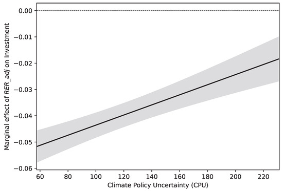
Figure 1 plots this marginal effect, ${\beta }_1+{\beta }_{3}CP{U}_t$, continuously across the observed range of the CPU index (57.6 to 231.3), together with the associated 95% confidence interval. The marginal effect is negative throughout the observed range and moves monotonically toward zero as CPU rises, consistent with an attenuating but not reversing relation between real-estate concentration and investment.

Figure 1. Marginal effect of $RER\text{\_}adj$ on investment across the CPU range. Note: Plots ${\beta }_1+{\beta }_{3}CP{U}_t$ from the column (3) specification of Table 4 across the observed range of the CPU index, with a shaded 95% confidence interval. The dashed line at zero marks the point at which the marginal effect of real-estate concentration on investment would vanish; the estimated effect remains negative throughout the observed range.

The most parsimonious interpretation is a structural floor rooted in asset commitment. Firms already concentrated in illiquid real estate enter each period with less discretionary capital expenditure. They were already investing at the low end of the distribution before CPU rose. When CPU rises, the uncertainty-induced real-options mechanism operates most forcefully on firms that had more new irreversible commitments available to delay. Firms at the high end of $RER\text{\_}adj$ have fewer such commitments and therefore bear a proportionally smaller share of the aggregate investment reduction. This mechanism is consistent with Kim and Kung (2017), who document that firms with less redeployable assets respond differently to uncertainty shocks than firms with more flexible capital, and with the irreversibility-based predictions of Bernanke (1983) and Dixit and Pindyck (1994) at the firm level.

This interpretation rests on a reduced-form interaction coefficient, not a structural estimate of a mechanism. The panel specifications control for industry and time effects and cluster standard errors at the firm level, but they do not exploit an instrument for CPU or a discontinuity in real-estate concentration. The evidence is consistent with the floor mechanism, but it cannot rule out alternatives. For instance, real-estate-heavy firms may simply be less responsive to macro conditions generally, or some unobserved characteristic correlated with $RER\text{\_}adj$ may drive the differential response.

Two features of the design narrow, though do not eliminate, these concerns. First, reverse causality from investment to $RER\text{\_}adj$ is an unlikely source of the interaction: $RER\text{\_}adj$ is built from the stock of gross buildings and land relative to gross PP&E, a slow-moving ratio shaped by decades of accumulated capital structure rather than the current period’s investment flow, and $CP{U}_t$ is a national, firm-invariant series that no single firm’s investment decision can plausibly move. It is difficult to construct a channel by which reverse causation would generate the interaction coefficient specifically, as opposed to simply the investment level. Second, the omitted-variable concern that some time-invariant firm characteristic correlated with $RER\text{\_}adj$ drives the differential response is addressed directly by the firm fixed-effects specification (Section 4.2), which absorbs any such confound and leaves the interaction intact; a residual confound would therefore have to co-move with $RER\text{\_}adj$ within firms over time and interact specifically with the national CPU series, a considerably narrower requirement than merely correlating with $RER\text{\_}adj$ in levels. As a further check, replacing the interaction term with $BaselineRE{R}_i\times CP{U}_t$, where $BaselineRE{R}_i$ is each firm’s real-estate concentration in its first sample year, fixed years before any observation used to estimate investment, while retaining contemporaneous $RER\text{\_}adj$ as a control, leaves the interaction positive and significant ($t=2.38$, reported in the additional specification-robustness checks in Section 4.6); the differential investment response to CPU is therefore not an artifact of using a contemporaneous measure of real-estate concentration.

A related alternative explanation is that the attenuation mechanically reflects firms with low baseline investment simply having less room left to fall, rather than a genuine asset-commitment floor. This is addressed using a pre-determined baseline-investment measure, each firm’s average investment rate over its first three sample years, sorted into quartiles. If the low-baseline-investment story were correct, the interaction should be concentrated among firms with the lowest baseline investment. Instead, the interaction is smallest and least significant in the lowest baseline-investment quartile ($t=1.47$) and largest and most significant in the highest baseline-investment quartile ($t=3.44$), and a triple interaction of $RER\text{\_}adj\times CPU\times$ High baseline investment is positive and significant ($t=2.06$). This pattern is the opposite of what a mechanical low-baseline-investment explanation predicts and is instead consistent with the asset-commitment floor binding hardest precisely among firms that otherwise had the most discretionary investment available to defer.

3.4. Economic Magnitude in Context

Using the indicator specification, the attenuation of the $RER\text{\_}adj$ effect on investment moving from low- to high-CPU years is 0.19 percentage points per standard deviation of $RER\text{\_}adj$ (from $-0.81$ to $-0.62$ percentage points of assets), representing a 23% narrowing of the investment gap between asset-composition groups. Relative to the sample mean investment rate of 5.3%, this offset is economically meaningful at the firm level for capital budgeting purposes.

Returning to the continuous specification, the main effect of $RER\text{\_}adj$ is never eliminated: even at the sample maximum of the CPU index (231.3), the marginal effect of a one-standard-deviation increase in $RER\text{\_}adj$ on investment remains negative at $-0.31$ percentage points. The floor mechanism attenuates but does not reverse the investment disadvantage of real-estate-heavy firms. Real-estate concentration is a persistent drag on investment regardless of the policy environment; climate policy uncertainty changes the size of that drag, not its direction.

3.5. Mechanism Discrimination: Financing Channels

The investment attenuation documented above is consistent with an asset-commitment floor, but it could still be accompanied by financing adjustments. Distinguishing the dominant real-side margin from any balance-sheet overlay is therefore more informative than asking whether financing moves at all. Table 5 reports the financing regressions using the gross-denominator concentration measure and the baseline sample restrictions. The financing evidence is mixed and should be interpreted as complementary rather than exclusionary.

Table 5. CPU Interaction: Financing margins.

	Leverage		Net Debt Issuance		Cash Holdings
	Cont.	Ind.	Cont.	Ind.	Cont.	Ind.
$RER\text{\_}adj$	$0.0117$	−0.0358 **	$0.0023$	$-0.0055$	0.0092	0.0281 ***
	(0.44)	(−2.23)	(0.34)	(−1.34)	(0.61)	(3.17)
$RER\text{\_}adj\times CPU$	−0.000551 **	−0.0287	−0.000087	−0.0028	0.000280 **	0.0303 ***
	(−2.59)	(−1.57)	(−1.62)	(−0.48)	(2.17)	(2.76)
N	60,185	60,185	55,024	55,024	60,177	60,177

OLS; firm-clustered SEs; t-stats in parentheses; *** p < 0.01, ** p < 0.05; Cont. = continuous CPU (year FE included); Ind. = above-median CPU binary (year FE omitted); controls: $lnAT$, ROA, R&D, $PPE\text{\_}Assets$, industry FE. Net Debt Issuance $N=\mathrm{55,024}$ and Cash Holdings $N=\mathrm{60,177}$ are smaller than the $N=\mathrm{60,185}$ baseline for the reasons given in Table 2’s note (missing cash data; first-sample-year firms lacking a lagged debt observation for the net-debt-issuance difference).

Credit and leverage adjustment. If real-estate-heavy firms carried a pure collateral advantage under high CPU, one would expect them to sustain investment by borrowing more when uncertainty rises (Chaney et al. 2012; Kiyotaki and Moore 1997; Rampini and Viswanathan 2010). The leverage regressions show the opposite sign in the continuous specification: the $RER\text{\_}adj\times CPU$ interaction is negative at $-0.00055$ ($t=-2.59$). The indicator specification is also negative, though less precise ($-0.0287$, $t=-1.57$). This pattern is inconsistent with a story in which high-real-estate-concentration firms preserve investment during high-CPU periods by expanding leverage.

Cash and precautionary balance-sheet adjustment. Cash holdings move in the opposite direction. The continuous interaction in the cash regression is positive at $0.00028$ ($t=2.17$), and the indicator specification is also positive at $0.0303$ ($t=2.76$). This is consistent with a precautionary-savings motive under uncertainty (Gilchrist et al. 2014): firms build liquidity buffers when future financing conditions or investment opportunities are uncertain, rather than committing that liquidity to current capital expenditure, and the pattern here suggests some precautionary balance-sheet adjustment among real-estate-heavy firms when climate policy uncertainty is elevated. Net debt issuance, however, does not show a comparably strong pattern: the continuous interaction is $-0.000087$ ($t=-1.62$), and the indicator interaction is $-0.00276$ ($t=-0.48$). Taken together, the financing results suggest some conservatism in leverage and liquidity management, but not a coherent financing expansion that could mechanically account for the investment result.

The decisive diagnostic is whether financing variables absorb the investment interaction once they are included directly in the investment regression. They do not. In supplemental specifications estimated on the $N=\mathrm{55,018}$ subsample with non-missing net debt issuance, adding leverage, cash holdings, and net debt issuance as controls leaves the continuous $RER\text{\_}adj\times CPU$ interaction at $0.000170$ ($t=5.43$). Adding their interactions with CPU attenuates it only modestly further, to $0.000161$ ($t=5.16$). The reduction from the full-sample baseline ($t=5.88$, $N=\mathrm{60,185}$) thus reflects both the smaller sample and the additional controls; within the $N=\mathrm{55,018}$ subsample, the interaction is stable across both specifications. The central investment result therefore survives even when financing margins are allowed to co-move with climate policy uncertainty.

The financing evidence thus points to a more nuanced mechanism. The dominant adjustment still appears to operate through capital budgeting: firms with more real-estate-concentrated hard assets enter high-uncertainty periods with less discretionary investment left to defer. At the same time, these firms also exhibit some balance-sheet adjustment, especially lower leverage and higher cash. The mechanism is therefore best understood as an asset-commitment channel in investment with a secondary precautionary financing overlay, rather than as a pure financing story or a pure no-financing story. This also distinguishes the paper from the financial intermediation channel in Khalil and Strobel (2023), who study lending reallocation across carbon-intensive and low-carbon industries rather than firm-level investment responses conditional on asset composition. The direction of the leverage and cash results is also consistent with a broader cross-setting literature linking climate-related risk to more conservative capital structure, including firm-level physical climate risk (Ginglinger and Moreau 2023; Jiang et al. 2025) and discrete climate-policy regulatory shocks (Dang et al. 2023). These studies document the financing-side pattern using different countries and different risk measures; the contribution here is to show that, in the U.S. CPU setting studied in this paper, the financing adjustment is secondary to a real capital-budgeting response concentrated among firms with less real-estate-concentrated hard assets.

4. Robustness

The results of Section 3 rest on three main choices: the Gavriilidis CPU index, industry and year fixed effects, and the industry-adjusted real-estate concentration ratio. Section 4.1, Section 4.2, Section 4.3 and Section 4.4 examine these choices and add a sample split to assess stability across the pre- and post-Paris regimes. Section 4.5 reports additional checks on growth controls, measurement, and inference. Table 6 reports the CPU-measure robustness; Table 7 reports the main specification checks; Table A1 in the Appendix A reports the supplementary growth, measurement, and inference checks.

Table 6. Robustness: Alternative CPU index constructions.

CPU Measure	$\mathit{\beta }\left(\mathit{RER}\text{\_}\mathit{adj}\right)$	t	$\mathit{\beta }(\mathit{RER}\text{\_}\mathit{adj}\times \mathit{CPU})$	t	${\mathit{R}}^2$
Panel A: Continuous CPU (year FE included)
Gavriilidis (primary)	$-0.063$ ***	$-13.9$	$0.000192$ ***	$5.88$	0.424
Narrow-text	$-0.055$ ***	$-15.4$	$0.000089$ ***	$5.48$	0.424
Broad-text	$-0.060$ ***	$-13.9$	$0.000141$ ***	$5.47$	0.424
News narrow	$-0.058$ ***	$-13.8$	$0.000125$ ***	$5.15$	0.424
News broad	$-0.072$ ***	$-11.0$	$0.000254$ ***	$5.20$	0.423
Panel B: Indicator CPU (year FE replaced by CPU binary)
Gavriilidis (primary)	$-0.048$ ***	$-16.1$	$0.0113$ ***	$3.50$	0.406
Narrow-text	$-0.047$ ***	$-15.2$	$0.0106$ ***	$2.85$	0.407
Broad-text	$-0.047$ ***	$-15.1$	$0.0100$ ***	$2.70$	0.407
News narrow	$-0.047$ ***	$-15.2$	$0.0106$ ***	$2.85$	0.407
News broad	$-0.047$ ***	$-15.2$	$0.0106$ ***	$2.85$	0.407
Panel C: Shock indicator (unexpected CPU component)
CPU shock indicator †	$-0.047$ ***	$-17.5$	$0.000116$	$0.05$	0.407

OLS; $N=\mathrm{60,185}$ except Panel C ($N=\mathrm{52,707}$); firm-clustered SEs; *** $p<0.01$; controls: $lnAT$, ROA, R&D, $PPE\text{\_}Assets$, industry FE; Panel B replaces year FE with CPU binary; ^† Panel C uses CPU shock indicator, no year FE.

Table 7. Additional specification robustness.

Specification	$\mathit{\beta }\left(\mathit{RER}\text{\_}\mathit{adj}\right)$	t	$\mathit{\beta }(\mathit{RER}\text{\_}\mathit{adj}\times \mathit{CPU})$	t	N	${\mathit{R}}^2$
Baseline (industry + year FE)	$-0.063$ ***	$-13.9$	$0.000192$ ***	$5.88$	60,185	0.424
Firm FE + year FE	$-0.063$ ***	$-10.0$	$0.000167$ ***	$4.21$	60,185	0.632
Post-Paris subsample (2016–2024)	$-0.077$ ***	$-6.86$	$0.000281$ ***	$4.95$	13,433	0.411
Pre-Paris subsample (1990–2015)	$-0.047$ ***	$-5.46$	$-0.000017$	$-0.17$	46,752	0.421
Raw $RER$ (unadjusted)	$-0.054$ ***	$-12.73$	$0.000129$ ***	$4.09$	60,185	0.423
Predetermined: $BaselineRER\times CPU$ (RER_adj retained)	$-0.044$ ***	$-10.78$	$0.0048$ **	$2.38$	60,185	0.631
Industry-year FE	$-0.063$ ***	$-14.2$	$0.000197$ ***	$6.36$	60,185	0.468
Dynamic (lagged Investment control)	$-0.034$ ***	$-13.6$	$0.0000954$ ***	$5.18$	54,954	0.608
Alt. investment: Capex/lagged Assets	$-0.072$ ***	$-12.0$	$0.000214$ ***	$5.08$	54,954	0.344
Alt. investment: (Capex + R&D)/Assets	$-0.057$ ***	$-7.94$	$0.000238$ ***	$4.27$	60,185	0.274
Tighter winsorization (2%/98%)	$-0.063$ ***	$-14.6$	$0.000196$ ***	$6.29$	60,185	0.439

OLS; dep. var. = Investment (Capex/Assets), except the two alternative-investment-measure rows, whose dependent variables are Capex/lagged Assets and (Capex + R&D)/Assets respectively; continuous Gavriilidis CPU with year FE; controls: ln AT, ROA, R&D, PPE_Assets, industry FE (except firm-FE and industry-year-FE rows; the (Capex + R&D)/Assets row omits the R&D control since R&D is already embedded in the dependent variable); firm-clustered SEs; *** p < 0.01, ** p < 0.05. Supplementary growth, measurement, and inference robustness checks are reported in Table A1 in the Appendix A. In the “Predetermined” row, the reported interaction is BaselineRER_i × CPU_t, not RER_adj × CPU: BaselineRER_i is each firm’s real-estate concentration in its first sample year, held fixed over time, CPU is standardized to unit variance for numerical conditioning of the firm-fixed-effects design matrix, and the specification includes firm and year fixed effects with contemporaneous RER_adj retained as a control (its coefficient and t-statistic are reported in the first two columns of that row).

4.1. Alternative CPU Measures

A natural concern is that the interaction result is sensitive to how climate policy uncertainty is measured. The Gavriilidis index is constructed from a specific keyword list and newspaper corpus; a different construction could produce a different time series of CPU and thereby a different interaction. That concern is standard in text-based uncertainty measurement, where alternative term dictionaries and source sets can alter the level and persistence of the resulting index (Baker et al. 2016; Gavriilidis 2021). Table 6 addresses this by replacing the primary index with four alternatives that span a meaningful range of construction choices.

The five indices differ along two dimensions. The first is text scope: the narrow-text index counts articles containing a tightly defined set of climate and policy keywords, while the broad-text index casts a wider net. The second is source: the cpnews variants are based on news coverage intensity rather than the broader editorial and opinion content that enters the primary index. These distinctions matter because a narrow keyword list will miss some relevant policy debates, while a broad list may admit noise from articles that mention climate and policy in unrelated contexts. A robust result should be insensitive to these design choices.

The evidence in Table 6 supports this. For continuous CPU specifications, t-statistics on the interaction range from $5.15$ to $5.88$ across all five indices. For high-CPU indicator specifications, t-statistics range from $2.70$ to $3.50$. The direction and significance of the interaction are invariant to the choice of index. In the indicator specification, the narrow-text, news-narrow, and news-broad indices produce similar interaction estimates (${\widehat{\beta }}_3\approx 0.0106$, $t\approx 2.85$ in each case). This is because these three indices are sufficiently correlated in levels that the binary above-median classification identifies the same set of high-CPU years. The replication of the result across this common timing is itself informative: any construction that assigns years to the high-CPU regime in the same way recovers the same differential investment response.

A supplemental specification replaces the level CPU measure with a binary indicator for above-median CPU shocks (the unexpected component of the Gavriilidis index, as described in Section 2.4). This specification is estimated on a smaller sample because the shock series is available for fewer firm-years. It yields a null interaction (${\widehat{\beta }}_3=0.0001$, $t=0.05$; Table 6 Panel C), indicating that the interaction documented in Section 3 is specific to the sustained level of climate policy uncertainty rather than discrete surprise shocks. This level-versus-shock distinction is consistent with the floor mechanism proposed in Section 3.3 rather than evidence against it. The asset-commitment floor describes the position of a firm’s discretionary investment capacity relative to its real-estate-concentrated hard-asset base, a slow-moving state that does not change because the current year happens to register an unexpected jump in policy risk. A firm that has already committed most of its capital budget to illiquid real estate has little additional room to cut regardless of whether uncertainty is high because of a discrete shock or because it has settled at a persistently elevated level; the mechanism instead operates through the sustained elevation of the uncertainty regime, which changes the option value of the marginal unit of remaining discretionary investment across many years rather than in response to a single surprise. A null shock coefficient cannot by itself identify which feature of CPU drives the result; it can only fail to contradict a given interpretation. With that caveat, the null shock result is more naturally read as consistent with the mechanism operating on the sustained level of CPU rather than its innovation, and it does not constitute evidence against the mechanism itself.

4.2. Within-Firm Identification

The baseline specification uses industry fixed effects to control for permanent differences across sectors and year fixed effects to control for aggregate time trends. A stricter benchmark replaces industry fixed effects with firm fixed effects, absorbing all time-invariant firm characteristics, including persistent differences in business model, ownership structure, and financing that might be correlated with real-estate concentration and with investment sensitivity to macroeconomic conditions.

Row 2 of Table 7 reports this within-firm specification. The interaction remains positive and significant: ${\widehat{\beta }}_3=0.000167$ with $t=4.21$, compared with $t=5.88$ in the baseline. The interaction is identified by the covariance of within-firm changes in $RER\text{\_}adj$ over time with the time-series of CPU. That the estimate remains significant under firm fixed effects reduces concern that the baseline result is upward-biased by between-firm heterogeneity. Firms whose real-estate concentration rises relative to the prior period invest less than their own historical norm when CPU is high, consistent with the baseline interaction documented in Section 3.

4.3. Sample Period Splits: Pre- and Post-Paris

The Paris Agreement of December 2015 constitutes a structural shift in the salience and institutional weight of climate policy. Before Paris, climate policy uncertainty largely reflected domestic legislative cycles and international negotiations. After Paris, it reflects the salience, persistence, and decision-relevance of nationally determined contribution targets, the evolving carbon pricing landscape across major economies, and the acceleration of climate-risk pricing in financial markets (Bolton and Kacperczyk 2021; Ilhan et al. 2021; Sautner et al. 2023). This matters because the mechanism in Section 3 should be most visible when policy uncertainty is high. The annual mean CPU is 193.1 in the post-Paris period, more than double the pre-Paris mean of 80.7.

Rows 3 and 4 of Table 7 split the sample at 2016. In the post-Paris subsample (13,433 observations), the interaction is positive and significant ($t=4.95$), despite the much smaller sample and the compression of the CPU distribution (all years are in the high-CPU regime by historical standards, reducing the time-series variation that identifies the interaction). In the pre-Paris subsample (46,752 observations), the interaction is close to zero and statistically indistinguishable from zero ($t=-0.17$).

This subsample comparison is suggestive but is not, by itself, a formal test of a discontinuity at 2016: comparing two subsample t-statistics does not distinguish a genuine break from a smooth trend that simply has more identifying variation in the later, higher-CPU years. That distinction was tested directly in two ways. First, a single pooled specification interacting $RER\text{\_}adj\times CPU$ with a post-2016 indicator yields a triple-interaction coefficient of $0.0000767$ ($t=1.69$), below conventional significance; allowing the interaction to also follow a smooth linear trend and testing whether a discrete jump remains on top of that trend leaves the jump term smaller still ($t=1.34$). Second, a complementary test uses each firm’s predetermined real-estate concentration interacted with calendar-year effects, deliberately excluding CPU from the specification to avoid its collinearity with calendar time; this shows a strong, smooth, monotonic trend in the RER-investment relationship across the full 1990–2024 sample ($t=5.14$) with no additional discontinuity at 2016 ($t=-0.25$, robust to excluding the 2020–2021 COVID years).

Together, these tests indicate that the empirical pattern is better described as a continuous strengthening of the interaction as climate policy uncertainty itself has risen and become more volatile, rather than a discrete break triggered by the Paris Agreement specifically. This is consistent with the CPU index nearly doubling in mean level from the pre-2016 to the post-2016 period (80.7 to 193.1) through a gradual accumulation of climate-policy salience rather than a single event. The pre/post-2016 comparison in Table 7 is retained as a useful descriptive regime comparison, since it corresponds to a widely recognized shift in the policy environment, but it is not interpreted as evidence of a structural trigger at the Paris Agreement specifically, and neither Bernanke (1983) nor Dixit and Pindyck (1994) predicts a discontinuity at a particular calendar date in the first place; the real-options framework predicts that attenuation should be more visible when uncertainty is higher and more persistent, which is the pattern the data show.

4.4. Industry Adjustment of the Real-Estate Measure

The primary measure, $RER\text{\_}adj$, subtracts the industry-year mean from each firm’s raw real-estate share. This adjustment removes cross-industry differences in real-estate intensity, which could otherwise allow industry effects to masquerade as a firm-level composition mechanism. A skeptic might argue that the adjustment is too aggressive, in the sense that much of the genuine variation is across industries and that removing it attenuates the result.

Row 5 of Table 7 uses the raw, unadjusted $RER$ in place of $RER\text{\_}adj$. The interaction remains positive and significant ($t=4.09$), with a coefficient somewhat smaller than the adjusted baseline ($0.000129$ versus $0.000192$). The main effect of raw $RER$ on investment is also negative ($-0.054$, $t=-12.73$), consistent with the adjusted measure. The industry adjustment therefore does not appear to create or eliminate the result: the interaction signal is present in the full cross-sectional variation in real-estate concentration, not just the within-industry component. Industry fixed effects already absorb industry-average real-estate intensity, so the additional adjustment in $RER\text{\_}adj$ is useful but not essential for interpretation.

4.5. Measurement, Growth Controls, and Inference

Three additional checks address the most natural residual concerns about the baseline specification; Table A1 in Appendix A reports these estimates. First, the interaction is robust to standard growth-opportunity controls. Adding firm-level sales growth leaves the interaction at $0.000185$ ($t=5.78$) on the subsample of $N=\mathrm{54,756}$ firm-years with a non-missing prior-year sales figure. Adding market-characteristic controls, namely $lnME$ and book-to-market, reduces the estimate but does not eliminate it: the interaction remains positive at $0.000163$ ($t=4.91$; $N=\mathrm{39,505}$), and when sales growth is included alongside these controls, it remains $0.000153$ ($t=4.78$; $N=\mathrm{38,418}$). The sample reduction under market-characteristic controls, roughly 35% below the full-sample baseline, is driven by firms without Compustat market data, which are predominantly smaller and less actively traded. The reduction from the full-sample baseline ($t=5.88$, $N=\mathrm{60,185}$) thus reflects both the restricted samples and the additional controls; within the $N\approx \mathrm{39,000}$ market-characteristics subsample, the interaction is stable across both growth-control configurations. The differential investment response to CPU is therefore not explained by a simple low-growth or maturity proxy story.

Second, the baseline interaction also survives direct measurement-related controls tied to the book-value construction of $RER$. Adding firm age and its interaction with CPU leaves the estimate at $0.000194$ ($t=6.00$). Adding the accumulated-depreciation ratio $\mathtt{dpact}/\mathtt{ppegt}$ and its interaction with CPU changes the coefficient to $0.000269$ while leaving it strongly significant ($t=8.04$). This increase is consistent with the floor mechanism rather than a specification artifact: the depreciation ratio proxies for how far a firm’s real-estate stock is through its useful life, and more heavily depreciated buildings are, if anything, less liquid and less readily repurposed than newer ones, so conditioning on depreciation stage removes measurement noise in the illiquidity signal carried by $RER\text{\_}adj$ rather than introducing a new confound. When firm age, the depreciation ratio, and the cap-hit indicator for observations where the raw gross-over-net ratio would exceed one are included jointly, the interaction remains positive at $0.000295$ with $t=7.62$. The age and cap-hit interactions are themselves not reliably different from zero, reducing concern that the main estimate is mechanically driven by older or more heavily depreciated capital stocks.

Third, inference is robust to stricter standard-error treatment: re-estimating the baseline continuous CPU specification with firm-and-year two-way clustered standard errors lowers the interaction t-statistic from $5.88$ to $5.55$, while leaving the coefficient unchanged. Taken together, these checks suggest that the main interaction is not an artifact of the particular control set, the omission of simple growth controls, or overly permissive one-way clustering.

4.6. Additional Robustness: Fixed-Effects Structure, Dynamics, Investment Measurement, and Redeployability

Four further checks address specification concerns not covered above. First, replacing the additive industry and year fixed effects with fully interacted industry-year fixed effects, which absorb any industry-specific shock common to all firms in that industry-year, leaves the interaction essentially unchanged (${\widehat{\beta }}_3=0.000197$, $t=6.36$). Second, a dynamic specification adding lagged investment as a control (a partial-adjustment-style check, not a full dynamic-panel GMM estimator) shows the interaction survives controlling for investment persistence (${\widehat{\beta }}_3=0.0000954$, $t=5.18$), with a highly persistent lagged-investment coefficient (0.51, $t=61.8$). Third, two alternative investment measures confirm the result is not specific to the primary definition: capital expenditure scaled by lagged rather than contemporaneous total assets, which addresses mechanical contemporaneous-denominator concerns (${\widehat{\beta }}_3=0.000214$, $t=5.08$), and capital expenditure plus R&D scaled by assets (${\widehat{\beta }}_3=0.000238$, $t=4.27$). Fourth, tightening the winsorization thresholds from 1st/99th to 2nd/98th percentiles leaves the interaction essentially unchanged (${\widehat{\beta }}_3=0.000196$, $t=6.29$); the replication package retains only already-winsorized ratio variables rather than raw Compustat components, so only tighter thresholds could be tested, and loosening the thresholds is left as a disclosed limitation rather than worked around.

A fifth, exploratory check tests the asset-commitment floor mechanism more directly by asking whether the interaction varies with the flexibility of a firm’s non-real-estate capital, using each firm’s predetermined operating-lease intensity ($\mathit{xrent}/at$, averaged over its first three sample years) as a proxy: firms that lease more of their operating space have an outside option that owned-real-estate-heavy firms lack, so the floor mechanism predicts a weaker interaction among high-lease-intensity firms. This prediction is not supported: a triple interaction of $RER\text{\_}adj\times CPU\times$ low lease intensity is small and only marginally significant, and in the opposite direction from the prediction ($t=-1.75$). This test is reported as an inconclusive, exploratory check rather than confirmatory evidence for or against the mechanism; the stronger mechanism evidence remains the firm-fixed-effects result (Section 4.2) and the baseline-investment-quartile test reported above, both of which show the pattern predicted by the floor mechanism and the opposite of what the leading mechanical alternative predicts.

5. Conclusions

This paper studies whether climate policy uncertainty transmits uniformly across firms or whether the composition of the hard-asset base shapes the response. Using a panel of 60,185 firm-year observations for U.S. nonfinancial firms from 1990 to 2024, it measures real-estate concentration as the share of gross PP&E held in buildings and land, adjusted relative to two-digit SIC industry-year peers. These arguments and results can be summarized as three hypotheses. H1 (baseline rigidity): $RER\text{\_}adj$ is negatively associated with investment, holding total tangible-capital intensity fixed; this is supported ($\beta =-0.042$, $t=-18.3$). H2 (attenuation under uncertainty): the negative association in H1 is attenuated when climate policy uncertainty is elevated; this is supported (${\beta }_{interaction}=0.000192$, $t=5.88$), and the attenuation strengthens continuously as CPU itself rises and becomes more volatile rather than appearing as a discrete break at any single calendar date. H3 (capital-budgeting margin): the attenuation in H2 operates primarily through real investment rather than financing adjustment; this is also supported, since leverage interactions are negative, cash rises modestly in high-CPU periods, and adding financing variables directly to the investment regression leaves the core interaction largely unchanged.

The paper’s contribution can be stated in three parts. First, it identifies real-estate concentration within the hard-asset base as a previously unexamined, within-industry source of heterogeneity in how climate policy uncertainty transmits to corporate investment (H1–H2), distinct from the aggregate policy shocks, financing constraints, and industry membership emphasized in prior work. Second, it shows this heterogeneity operates through a real capital-budgeting margin rather than financing (H3), and that it is not a fragile artifact of a single proxy, sample period, or control set: the interaction survives industry, firm, and industry-year fixed effects, a dynamic specification with lagged investment, alternative investment measures, alternative CPU indices, and stricter winsorization and clustering. Third, it contributes a firm-level, financial-statement-observable heterogeneity dimension to the climate-risk literature, alongside industry membership and firm-level text-based exposure measures used elsewhere. Real-estate concentration is observable from standard financial statements and helps identify which firms’ capital programs are likely to adjust differently when transition uncertainty rises.

The practical implications differ by stakeholder. For corporate managers, the asset-commitment floor implies that firms with real-estate-heavy balance sheets have comparatively little room to further compress investment as a hedge against rising CPU, so precautionary adjustment on the financing side, such as building cash or reducing leverage, may be a more relevant lever than further capital-expenditure deferral. For investors and lenders, real-estate concentration is an easily observable, financial-statement-based screen for identifying which firms’ investment programs are least sensitive to transition-policy uncertainty, independent of industry classification; firms that appear similar on industry screens may still differ materially in the flexibility of their investment response because their hard-asset composition differs. For policymakers, the result implies that the real economic impact of climate policy uncertainty is not distributed uniformly even within an industry: firms with more redeployable asset bases bear a disproportionate share of any uncertainty-induced investment slowdown, which is relevant for calibrating the timing and predictability of climate-related policy itself.

Several limitations remain. The design is reduced-form and associational; a credible instrument for either real-estate concentration or climate policy uncertainty is not available, so causal identification is not claimed. An exploratory test using predetermined lease intensity as a proxy for non-real-estate capital flexibility did not cleanly discriminate the proposed mechanism from alternatives, and is reported as inconclusive rather than confirmatory (Section 4.6). The sample is limited to U.S. nonfinancial firms, so external validity to other institutional settings remains open. The real-estate concentration measure also has known limitations: it is constructed from book-value gross PP&E rather than market values, so it does not capture unrealized appreciation or depreciation in the underlying real estate; the measure pools fatb and fatp into a single ratio by construction, since the paper’s interest is in the combined footprint of illiquid, difficult-to-redeploy hard assets rather than in separating buildings from land, which may have different adjustment costs and different climate exposures;2 and the measure captures owned real estate only, so firms that substitute toward leased space, which would not appear as a reduction in $RER\text{\_}adj$ but could reflect a similar underlying flexibility preference, are not distinguished from firms with genuinely lower real-estate intensity. The analysis also does not directly incorporate firm-level carbon intensity or property-level geographic exposure; if real-estate-heavy firms are also more carbon-intensive within industries, part of the estimated interaction could reflect a lending-reallocation channel operating alongside the real capital-budgeting margin studied here, a possibility that would not contradict the present results mechanically, since that literature studies lending composition rather than firm-level investment and balance-sheet outcomes, but would narrow the interpretation of the channel. If property portfolios differ systematically in local physical or regulatory risk, a single scalar measure of real-estate concentration will necessarily miss that dimension. Future work extending the analysis with a credible identification strategy, carbon-intensity controls, location-based physical and transition risk data, and a direct redeployability measure for non-real-estate capital would sharpen the interpretation and help connect the asset-composition channel documented here to the broader climate-risk measurement agenda.

References

- Baker, Scott R., Nicholas Bloom, and Steven J. Davis. 2016. Measuring economic policy uncertainty. Quarterly Journal of Economics 131: 1593–636. [Google Scholar] [CrossRef] [Scilit]
- Baldauf, Markus, Lorenzo Garlappi, and Constantine Yannelis. 2020. Does climate change affect real estate prices? Only if you believe in it. Review of Financial Studies 33: 1256–95. [Google Scholar] [CrossRef] [Scilit]
- Barnett, Michael, William Brock, and Lars Peter Hansen. 2020. Pricing uncertainty induced by climate change. Review of Financial Studies 33: 1024–66. [Google Scholar] [CrossRef] [Scilit]
- Bartram, Soehnke M., Kewei Hou, and Sehoon Kim. 2022. Real effects of climate policy: Financial constraints and spillovers. Journal of Financial Economics 143: 668–96. [Google Scholar] [CrossRef] [Scilit]
- Bernanke, Ben S. 1983. Irreversibility, uncertainty, and cyclical investment. Quarterly Journal of Economics 98: 85–106. [Google Scholar] [CrossRef] [Scilit]
- Bloom, Nicholas. 2009. The impact of uncertainty shocks. Econometrica 77: 623–85. [Google Scholar] [CrossRef] [Scilit]
- Bolton, Patrick, and Marcin Kacperczyk. 2021. Do investors care about carbon risk? Journal of Financial Economics 142: 517–49. [Google Scholar] [CrossRef] [Scilit]
- Chaney, Thomas, David Sraer, and David Thesmar. 2012. The collateral channel: How real estate shocks affect corporate investment. American Economic Review 102: 2381–409. [Google Scholar] [CrossRef] [Scilit]
- Cho, Chulyoung, Jinseok Yang, and Beakcheol Jang. 2024. Climate policy uncertainty and its impact on real estate market dynamics: A sectoral and regional analysis. PLoS ONE 19: e0311688. [Google Scholar] [CrossRef] [Scilit] [PubMed]
- Dang, Viet Anh, Ning Gao, and Tiancheng Yu. 2023. Climate policy risk and corporate financial decisions: Evidence from the nox budget trading program. Management Science 69: 7517–39. [Google Scholar] [CrossRef] [Scilit]
- Daumas, Louis. 2024. Financial stability, stranded assets and the low-carbon transition—A critical review of the theoretical and applied literatures. Journal of Economic Surveys 38: 601–716. [Google Scholar] [CrossRef] [Scilit]
- Dixit, Avinash K., and Robert S. Pindyck. 1994. Investment Under Uncertainty. Princeton: Princeton University Press. [Google Scholar]
- Gavriilidis, Konstantinos. 2021. Measuring Climate Policy Uncertainty. Working Paper. Stirling: University of Stirling. [Google Scholar]
- Giglio, Stefano, Matteo Maggiori, Krishna Rao, Johannes Stroebel, and Andreas Weber. 2021. Climate change and long-run discount rates: Evidence from real estate. Review of Financial Studies 34: 3527–71. [Google Scholar] [CrossRef] [Scilit]
- Gilchrist, Simon, Jae W. Sim, and Egon Zakrajsek. 2014. Uncertainty, Financial Frictions, and Investment Dynamics. NBER Working Paper No. 20038. Cambridge: NBER. [Google Scholar]
- Ginglinger, Edith, and Quentin Moreau. 2023. Climate risk and capital structure. Management Science 69: 7492–516. [Google Scholar] [CrossRef] [Scilit]
- Gulen, Huseyin, and Mihai Ion. 2016. Policy uncertainty and corporate investment. Review of Financial Studies 29: 523–64. [Google Scholar] [CrossRef] [Scilit]
- Ilhan, Emirhan, Zacharias Sautner, and Grigory Vilkov. 2021. Carbon tail risk. Review of Financial Studies 34: 1576–607. [Google Scholar] [CrossRef] [Scilit]
- Jiang, Chao, Youwei Li, Xinyue Zhang, and Yang Zhao. 2025. Climate risk and corporate debt decision. Journal of International Money and Finance 151: 103261. [Google Scholar] [CrossRef] [Scilit]
- Julio, Brandon, and Youngsuk Yook. 2012. Political uncertainty and corporate investment cycles. Journal of Finance 67: 45–83. [Google Scholar] [CrossRef] [Scilit]
- Kermani, Amir, and Yueran Ma. 2023. Asset specificity of nonfinancial firms. Quarterly Journal of Economics 138: 329–81. [Google Scholar] [CrossRef] [Scilit]
- Khalil, Makram, and Felix Strobel. 2023. Capital Reallocation Under Climate Policy Uncertainty. Discussion Paper 23/2023. Frankfurt am Main: Deutsche Bundesbank. [Google Scholar]
- Kim, Hyunseob, and Howard Kung. 2017. The asset redeployability channel: How uncertainty affects corporate investment. Review of Financial Studies 30: 245–80. [Google Scholar] [CrossRef] [Scilit]
- Kiyotaki, Nobuhiro, and John Moore. 1997. Credit cycles. Journal of Political Economy 105: 211–48. [Google Scholar] [CrossRef] [Scilit]
- Li, Qing, Hui Shan, Yuehua Tang, and Vincent Yao. 2024. Corporate climate risk: Measurements and responses. Review of Financial Studies 37: 1778–830. [Google Scholar] [CrossRef] [Scilit]
- Pankratz, Nora M., and Christoph M. Schiller. 2024. Climate change and adaptation in global supply-chain networks. Review of Financial Studies 37: 1729–77. [Google Scholar] [CrossRef] [Scilit]
- Rampini, Adriano, and S. Viswanathan. 2010. Collateral, risk management, and the distribution of debt capacity. Journal of Finance 65: 2293–2336. [Google Scholar] [CrossRef] [Scilit]
- Ren, Xiaohang, Xueyong Zhang, Cheng Yan, and Giray Gozgor. 2022. Climate policy uncertainty and firm-level total factor productivity: Evidence from china. Energy Economics 113: 106209. [Google Scholar] [CrossRef] [Scilit]
- Sautner, Zacharias, Laurence van Lent, Grigory Vilkov, and Ruishen Zhang. 2023. Firm-level climate change exposure. Journal of Finance 78: 1449–520. [Google Scholar] [CrossRef] [Scilit]
- Tuzel, Selale. 2010. Corporate real estate holdings and the cross-section of stock returns. Review of Financial Studies 23: 2231–69. [Google Scholar] [CrossRef] [Scilit]
Disclaimer/Publisher’s Note: The statements, opinions and data contained in all publications are solely those of the individual author(s) and contributor(s) and not of MDPI and/or the editor(s). MDPI and/or the editor(s) disclaim responsibility for any injury to people or property resulting from any ideas, methods, instructions or products referred to in the content. |
© 2026 by the author. Licensee MDPI, Basel, Switzerland. This article is an open access article distributed under the terms and conditions of the Creative Commons Attribution (CC BY) license.