


Abstract
Using daily data from Investing.com South Africa, this study investigates the forecasting performance of four Rand currency rate markets (EUR/ZAR, CHF/ZAR, BRL/ZAR, and CNY/ZAR) from 13 February 2018 until 24 February 2025. The predictive fitness of three competing models, Support Vector Regression (SVR), Principal Component Regression (PCR), and eXtreme Gradient Boosting (XGBoost), is explored between 80%/20% and 95%/5% training-testing splits. Forecasting accuracy is evaluated based on evaluation errors, i.e., Mean Absolute Error (MAE) and Root Mean Square Error (RMSE). The Diebold–Mariano test is employed to check for statistical significance. Empirical results show that the linear SVR model outperforms PCR across all markets, while XGBoost achieves competitive predictive accuracy on average; the trade-offs between SVR and XGBoost are often very small. The data indicate that linear kernel methods provide a robust prediction pipeline, especially when macroeconomic factors (gold, oil, platinum prices, and the USD/ZAR exchange rate) and calendar-based factors are taken into account, and offer a strong framework for predicting daily exchange rate fluctuations. The results of this research provide practitioners (traders, risk managers, and policymakers) with insights into the relative efficiency of the kernel vs. ensemble learning approaches for forecasting the value of emerging-market currencies in the presence of structural volatility.
1. Introduction
1.1. Forecasting of Currency Exchange Rates
After the collapse of the Bretton Woods system in the 1970s, forecasting financial time series, especially exchange rates, has become increasingly prominent in economics. According to Potgieter (2005), forecasting of exchange rates is important for international trade, risk management, and investment. As noted in Lothian (2001), exchange rates specify the relative worth of a pair of currencies. Meese and Rogoff (1983), which was one of the first studies to study exchange rate prediction and compare structural models (i.e., purchasing power parity, interest rate parity, monetary models, and so on) for exchange rate forecasting, their work was the first of its kind to compare them with a naive random walk. Known as the Meese–Rogoff puzzle, they found that failure to outperform the random walk model was due to their discovery. Researchers such as Mark (1995) and Cheung et al. (2005) extended these findings by combining previous studies. They established in their research and solidified the fact that traditional structural models are fundamentally ill-suited for the forecasting of exchange rate behaviour. Researchers pursuing improvements in forecasting performance had also explored using machine learning techniques to model nonlinear dynamics that structural models could not.
Several neural network variations have also been implemented in predictive analysis (Zheng et al. 2019). One of the earliest contributions was made by Zhang and Berardi (2001), which found that ensemble neural networks trained on multiple datasets outperformed single models in predicting the GBP/USD exchange rate. Expanding on such research He and Shen (2007), it was found that ensemble neural networks enhanced prediction accuracy for six currencies: Euro (EUR), Australian dollar (AUD), Canadian dollar (CAD), British pound (GBP), Japanese yen (JPY), and Swiss franc (CHF). Other researchers then examined ANNs’ potential more broadly. In Plasmans et al. (1998), ANNs could not yield a proper prediction of monthly exchange rates in an early stage. However, even with these initial failures, Panda and Narasimhan (2007) found that ANN methods outperformed conventional models in predicting exchange rate dynamics better than Choudhry et al. (2012), while Choudhry et al. (2012) found that bid/ask prices significantly affected ANN-based exchange rate prediction. Despite their promising prospects, most neural network studies are still challenged by the need for large datasets for stable performance (Ince and Trafalis 2006). This dependence is especially challenging in emerging market environments, where high-frequency, high-quality financial data are rare and characterised by structural discontinuities. Support Vector Regression (SVR) overcomes these shortcomings by providing strong theoretical guarantees, particularly convex optimisation guarantees of globally optimal solutions. It can efficiently generalise to smaller, noisy financial datasets, without the explicit large-sample requirement of ANN-based models (Tay and Cao 2001). Given data constraints and market-focused currency volatility, SVR’s theoretical advantage makes it an applicable method well-suited for predicting currencies like the South African Rand, where data constraints and the idiosyncratic volatility patterns of the market can hamper conventional modelling methods. Efficient prediction of exchange rates is therefore difficult due to the heterogeneous, nonstationary nature of financial data (Moosa 2016).
Emerging-market currencies like the South African Rand also face unique forecasting challenges that set them apart from other advanced-market currencies. These include high commodity price sensitivity and political risk pricing, with breaks in structure that follow. In addition, there are challenges posed by capital-market outflow swings driven by dynamic shifts in global risk sentiment, dynamics that models originally developed for the developed-market environment have not sufficiently accounted for (Ndlovu and Schaling 2018). This structurally different divergence demonstrates a gap in the literature; while SVR provides benefits for major currency pairs, its utility for ZAR-denominated pairs remains underexplored. As a result, we do not know whether the reported benefits of SVR extend beyond the currency treated with different volatility policies. Moreover, the period 2018-25 is significant for exchange rate forecasting studies, as it includes several structural breaks (e.g., the COVID-19 crisis) that induced idiosyncratic exchange rate instability in both developed and emerging markets (Chaudhary et al. 2020). As per Ryan (2023), the rand was one of the worst-affected emerging-market currencies during this period, losing value sharply relative to major currencies in early 2020 but recovering somewhat. Given that this period serves as natural stress testing of the forecasting model’s performance, it provides an opportunity to evaluate whether SVR produces stable predictions during extreme market turbulence.
1.2. Support Vector Regression in Forecasting Exchange Rates
Financial time series are among the most complex and difficult-to-predict phenomena owing to their high noise-to-signal ratio and nonstationarity Lu et al. (2009). Vapnik’s -insensitive loss function, Vapnik (1999), has made SVR a very efficient extension of Support Vector Machines (SVMs) for regression. Because SVR can capture nonlinear interactions with minimal sample sizes, it has attracted considerable interest among researchers in financial forecasting and has found strong application in exchange rate prediction. Several studies have assessed SVR forecasting and have generally reported similar results. Cao et al. (2005) also predicted daily fluctuations in USD/GBP using SVR. It was concluded that it can produce globally optimal predictions while reducing the risk of overfitting.
Tay and Cao (2001) showed the remarkable impact that small changes to SVR parameters can have on forecasting accuracy, emphasising that tuning hyperparameters is more important than default tuning. Yaohao and Albuquerque (2019) developed ninety different SVR models and observed that among them all kernel functions, such as Log, Cauchy, Stable Spline, etc., were generally better than the random walk benchmark. Bahramy and Crone (2013) reaffirmed the capability of SVR to handle the nonlinearity and nonstationarity of financial data. Although beneficial, Kim et al. (2002) observed that the predictive performance of SVR depended strongly on hyperparameter tuning, especially the kernel function and the regularisation parameter C. One key limitation of this body of literature has been the predominance of developed-market currency pairs.
Although the technical characteristics of SVR have been thoroughly explored and verified, the extent to which these factors can be consistently applied in emerging-market settings, where volatility shapes are fundamentally different, is unresolved. As one of the most actively traded emerging-market currencies, the South African rand offers arguably the most meaningful test case. Its response to commodity cycles, domestic political events, and shifts in global risk appetite creates a volatility regime not found in the G10 currencies, underpinning an established SVR forecasting framework. To fill this void, the current analysis applies SVR on four pairs denominated in ZAR. It systematically examines whether the methodological advantages found in developed-market contexts remain valid in emerging-market contexts. Because of its flexibility and high performance, as evidenced by empirical results across diverse datasets, the RBF kernel is one of the most popular kernels for exchange rate forecasting (Kim et al. 2002). However, recent results indicate a need for an empirical approach to selecting kernels rather than making a single choice. Non-standard kernels, such as Cauchy and Stable Spline, outperform RBFs on specific currency pairs, suggesting that their use should be an empirical decision rather than a predefined choice. This observation highlights a second uncharted territory in the literature: optimal kernel choice may depend not only on the dataset but also on the structural characteristics of the currency pair being predicted. We tackle this problem by evaluating kernel performance in four ZAR pairs of separate economic linkages: the euro for regional trade integration, the Swiss franc for safe-haven dynamics, the Brazilian real for commodity-driven emerging-market co-movement, and the Chinese yuan for policy-driven bilateral trade exposure, in an exploratory manner to see whether kernel selection interacts with regimes of volatility that matter more to currency.
To mitigate multicollinearity among input features, a problem in SVR-based exchange rate forecasting, researchers often adopt dimensionality reduction methods. Tay and Cao (2001) suggests using PCA, where closely correlated features are transformed into uncorrelated principal components, although much of the variance is retained to improve the model’s generalisation. Recursive Feature Elimination (RFE) (Kim and Shin 2007) is a second alternative approach to obtain predictors by picking the most significant ones and deleting similar predictors. This work adheres to these principles by incorporating dimensionality reduction into the modelling pipeline, thereby ensuring that multicollinearity does not disrupt SVR forecasting performance for the four ZAR pairs.
1.3. Principal Component Regression
Principal Component Regression (PCR) combines PCA with linear regression to address multicollinearity and overfitting (Jolliffe 2002). Correlated predictors are reduced to a smaller set of more orthogonal components that account for a larger share of the data’s variability and are included in the regression model. This approach is particularly suitable for predicting exchange rates since macroeconomic conditions and currency trends are often closely correlated (Jolliffe and Cadima 2016). Ponomareva et al. (2019) estimated the foreign exchange rate by using the PCR model. However, they found that PCA-based models were significantly better than random walks across several currencies, including the Australian dollar and British pound.
In another study, Ibekwe and Shiro (2022) demonstrated enhanced predictive ability by analysing the Nigerian Naira/USD exchange rate using PCA extracted from macroeconomic factors, one of the few works to apply dimensionality reduction to a newly introduced currency. This restriction is essential in emerging-market environments, where macroeconomic data-related variables, such as exchange rates, are frequently unstable due to structural breaks and fluctuating economic policy regimes. New approaches, e.g., guided PCR and sparse PCA, overcome these constraints by introducing supervised information in dimensionality reduction (Bair et al. 2006). The present study continues this methodological trend by using PCR not as a stand-alone forecasting model, but as a preprocessing step in the SVR framework, and by integrating the multicollinearity-reducing advantages of PCR with SVR’s ability to capture nonlinear relationships. The goal was not only to explore the same dimensionality reduction as in Ibekwe and Shiro (2022), but also to make our work applicable to four structurally distinct ZAR pairs and to assess whether the reduced dimensions generalise to other kinds of currency linkages being explored in emerging markets.
1.4. eXtreme Gradient Boosting
XGBoost (eXtreme Gradient Boosting) was introduced by Tianqi Chen and Carlos Guestrin in 2016 (Ge et al. 2022) and is an enhancement of the gradient boosting mechanism first described in (Aydin and Ozturk 2021). It is recognised as a highly efficient and scalable implementation of gradient boosting (Chen 2016), in which decision trees are constructed incrementally, with each tree correcting the prediction errors of the previous trees. XGBoost is widely known for its efficiency and robustness on structured or tabular datasets (Abir et al. 2024). Zhu (2023) highlights XGBoost’s feature selection and heterogeneous financial data management capabilities, whereas Raudys and Goldstein (2022) demonstrates that XGBoost performs more reliably in predicting financial price movements and volatility risk than traditional models.
The addition of XGBoost for this study contributes to a distinct methodological framework. SVR is a kernel-based method (suitable for processes with nonlinearity) that maps data to a high-dimensional feature space. In contrast, XGBoost is an ensemble-based method (which achieves nonlinearity via sequential error correction). Comparison of these two models within the same forecasting framework raises an unresolved question in the literature: whether the theoretical advantages of SVR (convex optimisation and global solution guarantees) are reflected in better empirical performance than ensemble methods that introduce nonlinearity via a fundamentally different mechanism. XGBoost provides greater interpretability using feature importance rankings than SVR and handles nonstationarity much more robustly thanks to its ensemble configuration. However, it requires careful tuning of multiple hyperparameters and can be prone to overfitting on smaller datasets. By using XGBoost as a benchmark model, this study provides a comparative view of kernel- and ensemble-based methods in the same emerging-market forecasting environment, thereby supporting the investigation of the interaction between methodological decision-making and the structure of the currency pair that may be forecasted.
1.5. Synthesis and Contribution to the Study
The first source listed in this literature review and three other related research gaps will be considered in the present paper. First, while SVR performs exceptionally well on developed-market currency pairs, much remains to be studied about emerging-market currencies, particularly the South African rand. Emerging-market currencies display a different structural profile than their G-10 counterparts, owing to their sensitivity to commodity prices, political risk, and shifts in global risk sentiment.
Second, the literature on SVR kernel selection already establishes that data dependency is an important factor in selecting an appropriate kernel type for an SVR model. However, none of those previous works has investigated whether kernel performance is influenced by the type of currency linkage to be forecasted. In this study, we bridge this gap by using a similar SVR model for predicting exchange rates of four currency pairs with markedly different economic relationships to South Africa (EUR/ZAR (regional trade integration), CHF/ZAR (safe-haven effects), BRL/ZAR (commodity-related co-movements in emerging markets), and CNY/ZAR (policy-driven trade relationships)).
Third, the studies have concentrated on the use of dimensionality reduction methods, including PCR, in developed countries or pairs of developing nations. This study adds to the findings by using a PCR-empowered SVR paradigm with four ZAR pairs. It allows for more comprehensive tests of whether the benefits of dimensionality reduction techniques are valid across categories of emerging-market currency pairs.
Table 1 summarises existing literature on exchange rate forecasting with five thematic streams. It shows that previous studies have found that one cannot beat random walk performance. However, new approaches such as neural networks and support vector regression techniques, as well as new technologies for selecting effective kernels, feature reduction techniques, and ensemble methods such as XGBoost, have benefited from more recent research. It also outlines the key authors in these thematic streams, their contributions, and the gaps that inspired this paper.
Table 1.
Summary of key literature by thematic stream.
1.6. Contribution and Research Highlights
This study adds scientific insight by comparing SVR performance with XGBoost and PCR across different ZAR-denominated currencies with distinct economic conditions.
The highlights of this study are:
- SVR with a linear kernel shows lower prediction errors (RMSE and MAE) for three out of four ZAR currency pairs (EUR/ZAR, BRL/ZAR, and CNY/ZAR), outperforming PCR and XGBoost.
- Diebold–Mariano (DM) test shows that SVR-Linear is more accurate than PCR on all four currency pairs (). This suggests that SVR has a greater capacity to capture nonlinear dynamics than linear dimensionality-reduction methods.
- The overall directional accuracy of 69.40%, along with very low RMSE (0.0125) and MAE (0.0099) of the CNY/ZAR pair, shows that an economical forecasting strategy of SVR-Linear is suitable for a dynamic exchange rate controlled pair such as this.
- Even though SVR-Linear produced lower point forecast error compared with the more complicated XGBoost model, DM results did not show statistically significant differences in forecasting accuracy in any of the four currency pairs. This provides a more robust level of statistical predictive power for the SVR-Linear. The POCID metric, which accounts for more than 65% of the change in direction predicted for the four currency pairs, suggests that predicting the short-term trend of emerging-market exchange rates is successful.
2. Models
2.1. Support Vector Regression
Support Vector Regression (SVR), proposed by Vapnik (1998), aims to estimate an unknown function from a training set , where and . The regression function is defined as
where denotes a nonlinear feature mapping, is the weight vector, and b is the bias term.
SVR minimises a regularised empirical risk using the -insensitive loss function
which leads to the following primal optimisation problem:
subject to
Introducing Lagrange multipliers and applying the Karush–Kuhn–Tucker conditions, the problem can be expressed in its dual form as
subject to
The optimal weight vector is given by
and the resulting SVR regression function can be written as
where denotes the kernel function. The SVR parameters are estimated by solving a convex quadratic programming problem, ensuring a unique global optimum (Smola and Schölkopf 2004).
2.2. Hyperparameter Tuning
This section describes the kernel functions used in SVR and the key hyperparameters that control model complexity and regularisation. Hyperparameter optimisation aims to identify optimal settings for the kernel, regularisation parameter C, and the epsilon , enabling SVR to effectively map input data into an appropriate feature space while achieving strong predictive performance and generalisation Vlok (2024).
2.2.1. Regularisation Parameter C
The regularisation parameter C controls the trade-off between model complexity and tolerance for errors beyond the -insensitive margin in SVR (Kamruzzaman et al. 2003). Larger values of C reduce regularisation and encourage closer fitting to the training data, increasing the risk of overfitting. In comparison, smaller values enhance regularisation, allowing greater deviations and potentially improving generalisation at the risk of underfitting (Tharwat 2019).
2.2.2. Epsilon-
A tolerance margin surrounding the predicted function is defined by the parameter in SVR. Data points that fall within this range are considered accurately predicted and do not affect the loss function. According to Wang et al. (2023), points outside the tube experience a loss proportionate to their distance from the boundary.
- Small : This results in a narrow -insensitive tube, which increases the risk of overfitting and makes the model sensitive to small deviations.
- Large : This results in a broad tube, which enables the model to ignore more significant deviations. This makes the model simpler and improves generalisation, but if significant patterns are ignored, it can lead to underfitting.
2.2.3. Gamma
In SVR, the gamma parameter is very important as it defines the role each data point plays for the model, especially when the Radial Basis Function (RBF) kernel is employed. A high gamma value makes the model highly sensitive to individual observations, leading to a complex, inconsistent regression function that overfits the training data and can generate noise rather than the underlying patterns (Devos et al. 2009). Lower gamma values increase the influence of each data point, resulting in a smoother, more generalised regression function that is less vulnerable to overfitting and better suited to identifying and displaying wider trends in the data.
2.2.4. Kernel Functions
Among kernel functions such as the sigmoid, polynomial, linear, and Radial Basis Function (RBF), these are among the most commonly used kernel functions in SVR. Each kernel is tailored to a particular data type according to dataset features (Vapnik 2013). The simplest of the four, we prefer using a linear kernel when the data are almost linearly separable. Moreover, in very clear visibility, it is the best choice to feature the target. The linear kernel can be precisely denoted as:
When the relationship between features and the target exhibits a polynomial pattern, the polynomial kernel can be particularly helpful. It requires selecting both the regularisation parameter C and the polynomial degree d. Adjusting the degree allows the model to match the complexity of the underlying data. The polynomial kernel is defined as:
The RBF kernel is the most commonly used in SVR, particularly when there is no prior knowledge about the underlying data distribution. It is capable of modelling complex, nonlinear relationships and often performs well across a wide range of problems (Shoko and Sigauke 2023). Two parameters must be specified for the RBF kernel: the regularisation parameter C and the kernel width parameter . The RBF kernel is defined as:
Finally, when the data exhibit a sigmoidal relationship, the sigmoid kernel, which is mathematically connected to neural network activation functions, is employed. The sigmoid function is defined as:
where is a hyperparameter controlling the scale of the input features.
2.3. Principal Component Regression Model
The benchmark model for this project is the principal component regression (PCR). PCR combines Principal Component Analysis (PCA) with linear regression to address multicollinearity by transforming correlated predictors into a reduced set of orthogonal principal components (Liu et al. 2003). These components capture most of the variance in the data and are used as regressors in the linear model
with the least squares estimator
PCA is obtained through eigenvalue decomposition or Singular Value Decomposition (SVD), where eigenvectors define component directions, and eigenvalues represent explained variance (Kerschen and Golinval 2002). To get the first b Principal Components (PCs), we can approximate the data matrix using Singular Value Decomposition (SVD):
where represents the low-rank approximation using the first b principal components, ) denotes the truncated SVD components, represents the principal component scores, represents the principal component loadings, and represents the residual matrix. Regressing on the scores leads to:
2.4. eXtreme Gradient Boost
The second benchmark model for this study is eXtreme Gradient Boosting (XGBoost). Gradient boosting is an ensemble learning technique in which decision trees are added iteratively to form a strong predictive model. At each iteration, a new tree is trained to minimise a specified loss function by fitting the residuals of the existing model (Abir et al. 2024). XGBoost constructs a predictive model in the form of an additive ensemble of decision trees, defined as
where denotes the predicted value, represents the k-th regression tree, K is the total number of trees, and is the input feature vector.
The model parameters are learned by minimising the following regularised objective function:
where is a differentiable loss function, and is a regularisation term that controls model complexity and prevents overfitting.
The regularisation term is defined as
where is the regularisation parameter and measures the complexity of the tree through its leaf weights.
To optimise the objective function, XGBoost applies a second-order Taylor expansion around the current prediction , yielding
where
represent the first- and second-order gradients of the loss function, respectively.
2.5. Evaluation Metrics
2.5.1. Mean Absolute Error
Mean absolute error (MAE) quantifies the average magnitude of errors in predictions. The equation for MAE is given by:
where denotes the predicted value from the model, represents the actual value, and n indicates the sample size. MAE uses the same scale as the data being evaluated. This is a scale-dependent accuracy metric; hence, it cannot be used to compare series with different scales Karunasingha (2022).
2.5.2. Root Mean Square Error
Root mean square error (RMSE) computes the square root of the average of squared errors. The formula for RMSE is as follows:
where n is the number of observations, is the actual value and is the predicted value.
2.6. Prediction of Directional Change
A main limitation of widely used evaluation indicators like RMSE and MAE is that they do not assess whether a model correctly captures the direction of changes in predicted values. The Prediction of Change in Direction (POCID) metric addresses this limitation. POCID tells us the ratio of the number of times the predicted direction matches the actual direction (Fallahtafti et al. 2022). POCID is defined as:
where m is the total number of forecast periods, and is the directional indicator denoted by:
This condition confirms whether the true change and the predicted one have the same sign. If both are positive or both negative, the prediction is correct (). Otherwise, we declare that it is wrong (). POCID analyses directional accuracy; however, it does not assess the magnitude of prediction distance to actual observations. Building on the proposed combined fitness metric (Fallahtafti et al. 2022) by integrating POCID and MSE, it has been proposed in this study that a composite metric should be developed, i.e., a combination of POCID and RMSE. This metric is a data-driven weight w, and it is defined as:
The weight w is computed as:
where k represents the number of models.
Thus, the final fitness metric becomes:
Higher values of the fitness metric indicate better model performance, reflecting both improved directional prediction and greater numerical accuracy.
2.7. Diebold–Mariano Test
Beyond standard forecast accuracy measures, this study uses the Diebold–Mariano (DM) test Diebold and Mariano (2002); Triacca (2018) to assess whether observed differences in forecasting performance across models are statistically significant rather than attributable to chance.
Let , for , denote the observed values of the exchange-rate series of interest. Let and represent the forecasts generated by two distinct models i and j, respectively, where and . The forecast error for model i is defined as:
Let denote a loss function applied to the forecast errors. In this study, squared error loss is employed, defined as
implying symmetric penalisation of forecast deviations. The loss differential between the two competing forecasts is then given by
The null hypothesis of the Diebold–Mariano test states that both models have equal predictive accuracy:
The alternative hypothesis indicates a statistically significant difference in forecasting performance:
2.8. Random Walk Model
The random walk model is a widely accepted benchmark in exchange rate forecasting, often employed to evaluate the relative effectiveness of more complicated models Meese and Rogoff (1983). Under the random walk assumption, the most recently observed value of the exchange rate provides the one-step-ahead forecast:
where denotes the forecast at time t, and is the observed value at time . In this study, the random walk model is applied to the raw exchange rate levels rather than the first-differenced series, meaning that the forecast at each period is simply the last observed exchange rate level. This approach is consistent with the original formulation of the random walk benchmark proposed by Meese and Rogoff (1983), in which the current level of the exchange rate is used directly as the forecast for the next period.
3. Empirical Results
3.1. Exploratory Data Analysis
3.1.1. Data Source
This study employs daily secondary data made publicly available on Investing.com’s website. The website is accessible at the following link: Investing.com (EUR/ZAR Historical Data) (https://za.investing.com/currencies/eur-zar-historical-data, accessed on 18 September 2025). The data range from 12 February 2018 to 24 February 2025. The data are collected over a five-day trading week.
3.1.2. Data Characteristics
To assess the effectiveness and reliability of machine learning models, the dataset is split into training and validation sets at 80% and 20%, respectively. This method allows you to evaluate the model’s consistency and ability to function well even with minimal training data. For exchange rate forecasting, where recent observations tend to carry the most predictive information, this method is particularly appropriate. The target variable for prediction is the first-differenced series of exchange rates, including Rand/Euro, Rand/CHF, Rand/BRL, and Rand/CNY, which serves as the response variable in the models.
where denotes the first difference at time t, is the closing price at time t, and is the closing price of the previous day.
The explanatory variables of the dataset are:
- difflag2: two-day lag difference between time t and time t-2 in the exchange rates.
- difflag5: five-day lag difference between time t and time t-5 in the exchange rates.
- diffUSD/ZAR: the first difference of the US dollar and the South African rand spot exchange rate.
- diffOilPrice (Brent crude): the first difference of the Brent crude oil spot price in USD per barrel.
- diffPlatPrice: the first difference of the international platinum spot price.
- diffGoldPrice: the first difference of the international gold spot price.
- Day: represents the day of the week.
- Month: represents the month of the year.
The covariates used in this model, which are gold, platinum, crude oil prices (Brent) and the USD/ZAR exchange rate, were obtained from the following website:
- Gold: https://www.investing.com/commodities/gold-historical-data (accessed on 18 September 2025).
- USD/ZAR exchange rate: https://www.investing.com/currencies/usd-zar (accessed on 18 September 2025).
- platinum: https://www.investing.com/commodities/platinum-historical-data (accessed on 18 September 2025).
- oil price(Brent crude): https://www.investing.com//brent-crude-historical-data (accessed on 18 September 2025).
3.1.3. Data Processing
Prior to model estimation, all variables were standardised to guarantee comparability across features with different scales. This was achieved using the scale = TRUE argument in the e1071 Support Vector Regression framework, which automatically normalises the predictors to zero mean and unit variance based on the training data Karatzoglou et al. (2006). The same scaling parameters were then applied to the test set for prediction, preventing data leakage and ensuring consistency between the training and assessment phases. Although each exchange rate was modelled separately, all series were initially synchronised to a common date index using the VLOOKUP function to ensure sample-period consistency and comparable forecasting performance across currency pairs. Missing observations from non-trading days were handled via forward-fill imputation to ensure a balanced dataset and maintain the continuity of the financial time series.
3.1.4. Dataset Description
Figure 1 below shows the performance of the rand against each of the euro, Swiss franc, Brazilian real, and Chinese yuan from 13 February 2018 through 24 February 2025. For all exchange rate pairs, a long-term upward trend indicates the rand’s depreciation relative to the respective currencies, with volatility varying markedly. The exchange rates were stable until 2020, then depreciated sharply and became more volatile during the COVID-19 pandemic, leading to increased volatility during global crises and to capital outflows from emerging markets. A partial recovery is visible during 2020–2021, but the period is again dominated by renewed and ongoing depreciation, particularly in the case of the euro and Swiss franc, and from 2022 onwards. Because volatility shows trends and clustering, the series are nonstationary and require differencing before forecasting.
Figure 1.
Rand/euro exchange rate plot (top left panel), rand/CHF exchange rate plot (top right panel), rand/BRL exchange rate plot (bottom left panel), rand/CNY exchange rate plot (bottom right panel).
3.1.5. Summary Statistics
Table 2 presents the descriptive statistics of the first-differenced exchange rate series for four ZAR currency pairs. All four pairs have means and medians nearly equal to zero, indicating that the differencing technique successfully removed the trend component from the data and that none of the pairs shows a significant, consistent appreciation or depreciation tendency. Significant volatility differences are observed across the pairings, with CHF/ZAR having the highest standard deviation (0.1525), followed closely by EUR/ZAR (0.1484), while BRL/ZAR (0.0337) and CNY/ZAR (0.0203) exhibit far lower volatility. All four currency pairs exhibit near-perfect quartile symmetry around zero, implying that the ZAR will appreciate and depreciate nearly equally. The four currency pairs show positive excess kurtosis, confirming leptokurtic distributions with fatter tails than the normal distribution. This supports the adoption of SVR, whose -insensitive loss function is assumed to be robust to outliers and extreme observations.
Table 2.
Descriptive statistics of the first difference series.
3.2. LASSO/Elastic Net Variable Selection
The first-difference series of the exchange rates can be modelled by selecting the most important predictors using regularised regression techniques, particularly LASSO and elastic net. These techniques perform automatic variable selection and lower the risk of overfitting, especially when predictors are numerous or correlated, by adding a penalty term to the regression objective, reducing coefficients, and setting some to zero (Zou and Hastie 2005). To effectively apply these techniques, R’s glmnet package can be utilised (Tibshirani 2014). Using coordinate descent and warm-start strategies, glmnet solves the penalised maximum-likelihood problem across a grid of regularisation parameters (). It supports ridge (), LASSO (), or elastic net () penalties.
The plot of cross-validation error versus alpha given in Figure 2 shows that the minimum cross-validation error of 0.01124, obtained during the tuning process for the EUR/ZAR pair, occurs at = 0.95 (red dot). This indicates that an elastic net model combining LASSO and ridge penalties provides the best predictive performance for this currency pair. The parameter places the model closer to the LASSO end of the regularisation spectrum while retaining a small but meaningful ridge component, suggesting that sparse variable selection is the primary regularisation requirement for the EUR/ZAR dataset, with modest coefficient reduction used to stabilise estimates among correlated predictors. This is particularly crucial in the EUR/ZAR context, where commodity prices such as gold and platinum are known to be correlated with one another and with lagged exchange rate movements, resulting in a form of multicollinearity structure that favours the elastic net over pure LASSO or ridge alone. Pure LASSO discards correlated but informative predictors, while pure ridge retains all predictors without eliminating irrelevant ones. The elastic net at = 0.95 strikes an optimal balance between these two extremes, achieving the lowest cross-validation error by combining aggressive variable selection with just enough coefficient shrinkage to handle correlated inputs effectively.
Figure 2.
CV Error vs. Alpha plot ( = 0.95).
The plots of cross-validation error versus alpha for the other currency pairs, BRL/ZAR, CHF/ZAR, and CNY/ZAR, are given in Figure A1, Figure A2 and Figure A3, respectively.
Table 3 displays the final elastic net coefficients at for all four ZAR currency pairs. The second lag of the differenced exchange rate (difflag2) is by far the most influential predictor across all pairs, with consistently large positive coefficients of 0.4852 for EUR, 0.4892 for BRL, 0.4778 for CHF, and 0.4726 for CNY, indicating that short-term autocorrelation is the primary driver of ZAR exchange rate movements in all four bilateral relationships. Several predictors were reduced to zero across all four pairs, including difflag5, diffUSD/ZAR, and Month, indicating that the fifth lag, the US dollar difference, and seasonal trends provide no useful predictive information for short-term ZAR exchange rate predictions. DiffPlatPrice, the only commodity price variable retained across all four pairs, displays negative coefficients in all cases, which is economically reasonable given South Africa’s status as the world’s largest platinum producer. diffOilPrice is retained only for the EUR/ZAR (−0.0041) and CHF/ZAR (−0.0057) pairs, implying that oil price movements have a greater influence on ZAR movements against developed-market currencies than against emerging market peers, whereas diffGolPrice is retained only for the BRL/ZAR pair (−0.0000843), possibly reflecting South Africa and Brazil’s shared sensitivity to gold price fluctuations. The Day variable is preserved only for the EUR/ZAR pair (−0.0013), indicating a little day-of-week effect that is absent from the other three pairs. Overall, the elastic net results indicate that ZAR exchange rate forecasting is predominantly influenced by short-term autocorrelation rather than macroeconomic fundamentals, with commodity prices having a secondary, market-specific impact.
Table 3.
Final LASSO coefficients at .
3.3. Linear Model Relative Importance
Table 4 shows the relative importance of predictors for the first-differenced exchange rate among all four ZAR currency pairs as calculated by the LMG (Lindeman, Merenda, and Gold) metric. The metric decomposes the full into non-negative contributions for each predictor. In this way, the results show that short-term autocorrelation dominates the predicted structure of the four markets, with most of the explained variance appearing in difflag2 per pair, with importance values between 0.6944 (CNY) and 0.7475 (BRL). The fifth lag (difflag5) comes in second for predictors for all pairs, with a coefficient of 0.2225–0.2323, indicating that short-term momentum rather than macroeconomic fundamentals mostly drives ZAR exchange rate variation. DiffPlatPrice emerges as the principal macroeconomic predictor across all pairs, with the strongest platinum price sensitivity for the CNY/ZAR pair (0.0649), consistent with China being one of the largest consumers of South African platinum exports. In comparison, diffOilPrice is more relevant for developed-market pairs than for emerging-market counterparts. All pairs have p-values less than 0.001 for the calendar variables Day and Month, suggesting no statistically significant seasonal or day-of-week effects on the ZAR exchange rate.
Table 4.
Relative importance of predictors for difflag1 (lmg metric).
3.4. Support Vector Regression
Table 5 presents the prediction performance of the SVR model on its four kernel functions and 4 ZAR currency pairs (80%/20% training-testing split). Because the best test RMSE and MAE come from the linear kernel in EUR/ZAR (RMSE = 0.0871 and MAE = 0.0676), BRL/ZAR (RMSE = 0.0872, MAE = 0.0676), CNY/ZAR (RMSE = 0.0125, MAE = 0.0099), and CHF/ZAR, it shows the best performance in all four markets. In most pairs, the radial kernel is the other best candidate with test RMSE values of 0.0919 (EUR), 0.0901 (BRL), 0.1104 (CHF), and 0.0131 (CNY), which indicate that it can replace the linear kernel (e.g., between the BRL/ZAR pair with negligible change of performance between them). The polynomial kernel is consistently outperformed by the linear and radial kernels across all four pairs and all three measures, ranking second among the leading factors of the largest errors after the sigmoid kernel in all cases. From the test RMSE values of 4.9291 (EUR), 7.4283 (BRL), 3.5026 (CHF), and 0.6432 (CNY), we can observe that the Sigmoid kernel performs significantly worse than all four of the other kernels between them, confirming that the Sigmoid kernel is not suitable for ZAR exchange rate prediction even when two other countries share a currency pair. CNY/ZAR shows even smaller absolute errors than any of the three total models, indicating the relatively low volatility and narrow range of exchange rates in the CNY/ZAR data. The ZAR-CHF pair consistently produced the greatest errors among the four pairs across all kernels, with a linear test RMSE of 0.1092 and an MAE of 0.0848; the latter showed greater volatility and a wider range, as noted earlier in the descriptive data. This finding is consistent with the observation that the linear and radial kernels exhibit relatively small train-test gaps when their RMSE values are compared; thus, they appear to generalise well without heavy overfitting. On the other hand, the gap for the polynomial kernel might be larger, suggesting some overfitting on the training data. Overall, the SVR results suggest that the linear kernel has the best short-term forecasting capability for ZAR exchange rate prediction across all four bilateral currency relations studied.
Table 5.
SVR model forecasting performance based on an 80%/20% training–testing split.
Table 6 shows the SVR model’s forecasting performance across four kernel functions and four ZAR currency pairs with a 95%/5% training–testing split. The linear kernel exhibits the lowest test RMSE and MAE in three of the four currency pairs, namely EUR/ZAR (RMSE: 0.0782, MAE: 0.0621), BRL/ZAR (RMSE: 0.0206, MAE: 0.0159), and CNY/ZAR (RMSE: 0.0112, MAE: 0.0089), confirming its constant dominance across these markets. The CHF/ZAR pair again presents an exception, with the radial kernel recording lower test RMSE (0.0878) and MAE (0.0663) than the linear kernel (RMSE: 0.0892, MAE: 0.0688), implying that the increased volatility of this pair favours a degree of nonlinear modelling that the linear kernel cannot fully capture. The Sigmoid kernel remains unfit across all four markets, with test RMSE values higher than those of the other kernels. Compared with the 80%/20% split results, all models have lower test errors at the 95% split across all four pairs, consistent with the anticipated improvement in forecasting accuracy as the volume of training data increases.
Table 6.
SVR model forecasting performance based on a 95%/5% training–testing split.
3.5. Principal Component Regression
The optimal number of components in the PCR model is determined using cross-validation, following the framework of Mevik and Wehrens (2015). The please package implements this procedure via the validation option, producing cross-validated prediction errors. To avoid subjective interpretation of validation plots, two objective criteria are employed: the one-sigma heuristic and the randomisation test. The one-sigma rule selects the most parsimonious model within one standard error of the minimum RMSEP, while the randomisation test assesses whether additional components yield statistically significant improvements.
Figure 3 and Figure 4 show the validation plots for the optimal number of components for training sets of 80% and 95%, respectively. The validation results for the 80% training split show that eight components are sufficient to account for the variation in difflag1. As the number of components increases, the RMSEP steadily decreases until it reaches a minimum at eight. The model’s stability and robustness are demonstrated by the accurate alignment of the CV and adjusted CV RMSEP curves.
Figure 3.
Validation plot showing optimal number of components for 80% training set.
Figure 4.
Validation plot showing optimal number of components for 95% training set.
PCR cross-validation results are summarised in Table 7 for two different training datasets: 80% and 95%. Both sets identify the number of 8 components as optimal. The dataset with 95% of the data shows a slightly lower cross-validation RMSEP (0.1079 vs. 0.1107), indicating that its predictions are slightly more accurate. In both cases, the explained variance in X equals 100%, while the explained variance in Y is around 49% (48.66% and 49.07%).
Table 7.
PCR Cross-Validation RMSEP and Variance Explained (X and Y) for the 80% Training Split.
Table 8 displays the PCR forecasting performance for four ZAR currency pairs with an 80% training split. The results exhibit impressively similar performance across all four markets, with RMSE values ranging from 0.09221 (BRL/ZAR) to 0.09463 (EUR/ZAR) and MAE values ranging from 0.07142 (BRL/ZAR) to 0.07355 (EUR/ZAR). The BRL/ZAR pair has the best forecasting performance of the four markets, with the lowest RMSE (0.09221) and MAE (0.07142), implying that the principal components extracted from macroeconomic predictors capture the underlying structure of the BRL/ZAR relationship more effectively than the other three pairs, possibly reflecting South Africa and Brazil’s shared commodity-dependent economic structures. The EUR/ZAR pair has the highest RMSE (0.09463) and MAE (0.07355) of the four pairs, indicating that the PCR model struggles most with the EUR/ZAR relationship, consistent with the higher volatility and broader range reported in the descriptive data. The CHF/ZAR and CNY/ZAR pairs perform very similarly, with RMSE values of 0.09446 and 0.09451 and MAE values of 0.07337 and 0.07339, respectively, indicating that the PCR model handles these two pairs with comparable effectiveness despite their fundamentally different volatility profiles, with the CHF/ZAR being highly volatile. The CNY/ZAR is the least volatile of the four pairs.
Table 8.
PCR forecasting performance for different markets at 80% training split.
The PCR forecasting performance for each of the four ZAR currency pairs at the 95% training split is shown in Table 9. With RMSE values ranging from 0.0858 (BRL/ZAR) to 0.0888 (EUR/ZAR) and MAE values ranging from 0.0687 (BRL/ZAR) to 0.0699 (EUR/ZAR), the results show a consistently narrow performance range across all four markets. The EUR/ZAR pair consistently records the highest errors, whereas the BRL/ZAR pair performs best, with the lowest RMSE and MAE across both the 80% and 95% splits. All four currency pairs show lower errors at the 95% split than at the 80% split, demonstrating that PCR forecasting accuracy increases with training sample size.
Table 9.
PCR forecasting performance for different markets at 95% training split.
3.6. eXtreme Gradient Boosting
Table 10 shows the predicting accuracy of the XGBoost model across four ZAR currency pairs, using 5-fold cross-validation with 1000 trees at the 80% training split. The findings show a consistent pattern of performance across all four markets, with RMSE values ranging from 0.09566 (BRL/ZAR) to 0.09839 (CNY/ZAR), and MAE values ranging from 0.07490 (EUR/ZAR) to 0.07822 (CNY/ZAR). Unlike the SVR and PCR findings, where the CNY/ZAR pair continuously recorded the lowest errors due to its low volatility, the XGBoost model performs poorly on the CNY/ZAR pair, with the highest RMSE (0.09839) and MAE (0.07822) among the four markets. This unexpected finding shows that XGBoost’s ensemble tree structure may be less effective at capturing the smooth, low-volatility dynamics of the regulated CNY/ZAR exchange rate than kernel-based SVR or PCR’s dimensionality-reduction technique. The BRL/ZAR pair has the lowest RMSE (0.09566), while the EUR/ZAR pair has the lowest MAE (0.07490), indicating that XGBoost works best on pairs with moderate and well-structured volatility patterns.
Table 10.
Forecasting accuracy of the XGBoost model across various markets employing 5-fold cross-validation with 1000 trees at 80% training split.
Table 11 displays the XGBoost forecasting performance across the four ZAR currency pairs at the 95% training split, employing 5-fold cross-validation with 1000 trees. With RMSE values ranging from 0.0823 (EUR/ZAR) to 0.0854 (BRL/ZAR), and MAE values between 0.0637 (BRL/ZAR) and 0.0688 (CNY/ZAR), indicating broadly comparable performance across all four markets. Compared to the 80% split, all pairs record lower errors at the 95% split, confirming that XGBoost accuracy improves consistently as the training sample increases.
Table 11.
Forecasting accuracy of the XGBoost model across various markets employing 5-fold cross-validation with 1000 trees at 95% training split.
3.7. Model Comparison
Forecasting Accuracy
Table 12 provides the forecast accuracy of the three respective prediction models, SVR-Linear, PCR, and XGBoost, considering the difference of ZAR in the currency pair used in an 80% training and 20% testing split. We provide a clear and consistent pattern of model performance across most markets, with SVR-Linear being the dominant forecasting model for three of the four currency pairs. For the EUR/ZAR pair, SVR-Linear produces the lowest RMSE (0.0871) and MAE (0.0676), followed by PCR (RMSE: 0.0946, MAE: 0.0736) and XGBoost (RMSE: 0.0958, MAE: 0.0749). Likewise, for the BRL/ZAR pair, SVR-Linear has the lowest RMSE (0.0872) and MAE (0.0676), with far superior RMSE and MAE than PCR (RMSE: 0.0922, MAE: 0.0714) and XGBoost (RMSE: 0.0957, MAE: 0.0758), further validating its superiority for this emerging market currency pair. The CNY/ZAR pair yields the most striking result, with SVR Linear recording an exceptionally low RMSE of 0.0125 and MAE of 0.0099, substantially lower than both PCR (RMSE: 0.0945, MAE: 0.0734) and XGBoost (RMSE: 0.0984, MAE: 0.0782), showcasing the low fluctuations and managed exchange rate dynamic of the CNY/ZAR pair and its combination of the CNY/ZAR pair and SVR-Linear model with the SVR-Linear kernel’s parsimonious model. The CHF/ZAR pair shows the least extreme result for SVR-Linear, indicating that the SVR-Linear model has the highest error rate (e.g., the lowest RMSE and the lowest MAE; PCR (0.0945, 0.0734), XGBoost (0.0963, 0.0757), and SVR-Linear have the worst error rate for the three models (RMSE; 0.1092, 0.0848; MAE; SVR-Linear). CHF/ZAR’s significantly higher volatility can potentially exceed the linear kernel’s limited ability to capture the general nonlinear dynamics, supporting the dimension-reducing strategy of PCR in this market. For all four combinations, XGBoost has the most significant errors among the three models of EUR/ZAR, BRL/ZAR, and CNY/ZAR, only being second for CHF/ZAR, which implies that the ensemble tree structure of XGBoost had little advantage over simpler SVR-Linear and PCR methods for short-term ZAR exchange rate prediction. In general, this outcome confirms that the SVR-Linear forecast is the most accurate short-term ZAR exchange rate prediction model for most bilateral currency pairs studied, and that it models nonstationary and nonlinear behaviour in emerging-market exchange rate data.
Table 12.
Forecast accuracy of competing models using an 80% training and 20% testing split.
Table 13 shows the forecast accuracy of three competing models across four ZAR currency pairs with a 95% training and 5% testing split. SVR-Linear has the lowest RMSE and MAE for three of the four currency pairs, confirming its consistent superiority over both benchmark models across both training splits. The CHF/ZAR pair again presents an exception, with both XGBoost (RMSE: 0.0847, MAE: 0.0674) and PCR (RMSE: 0.0887, MAE: 0.0697) outperforming SVR-Linear (RMSE: 0.0892, MAE: 0.0688). This suggests that the increased volatility of this pair continues to hinder the effectiveness of the linear kernel across training splits. A key finding at the 95% split is that XGBoost outperforms PCR across three of the four pairs, reversing the pattern seen at the 80% split and indicating that XGBoost’s ensemble structure becomes more effective as the training data volume increases. Overall, all three models record lower errors at the 95% split than at the 80% split across all four currency pairs, demonstrating that forecasting accuracy improves with larger training samples.
Table 13.
Forecast accuracy of competing models using a 95% training and 5% testing split.
3.8. Diebold–Mariano Test
We present the results from the Diebold–Mariano (DM) tests based on the 80% and 95% training splits. The models considered are M1 (SVR-Linear), M2 (PCR), and M3 (XGBoost). The null hypothesis is:
H0:
Forecasts from the two competing models are equally accurate.
H1:
The two competing models have different accuracies.
Table 14 presents the Diebold–Mariano (DM) test statistics comparing the forecast accuracy of SVR-Linear against PCR and XGBoost for the four ZAR currency pairs at both the 80% and 95% training splits, where a negative test statistic indicates that SVR-Linear produces lower forecast errors than the competing model. SVR-Linear considerably outperforms PCR across all four currency pairs at the 80% split, with DM statistics of −3.84 () for EUR/ZAR, −3.77 () for CHF/ZAR, −2.88 () for BRL/ZAR, and −3.77 () for CNY/ZAR, all falling well below the conventional 5% significance threshold. This pattern is maintained at the 95% split, where DM statistics of −3.25 () for EUR/ZAR, −3.20 () for CHF/ZAR, −2.84 () for BRL/ZAR, and −3.21 () for CNY/ZAR again confirm SVR-Linear’s statistically significant superiority over PCR across all four markets, demonstrating that this finding is robust to the choice of training split. Despite PCR recording marginally lower point forecast errors than SVR-Linear for the CHF/ZAR pair at both splits, the DM test statistics of −3.77 () at the 80% split and −3.20 () at the 95% split consistently confirm SVR-Linear’s statistical superiority for this pair, indicating that SVR-Linear’s overall forecast error distribution is statistically superior to that of PCR when evaluated over the full test period regardless of the training configuration used. These results collectively confirm that SVR-Linear outperforms PCR across all four bilateral currency pairs and that SVR’s kernel-based framework is better equipped to capture the nonlinear dynamics of emerging-market exchange rate data than PCR’s linear dimensionality-reduction approach. By contrast, the DM test reveals no statistically significant difference in forecasting performance between SVR-Linear and XGBoost across any of the four pairs at either training split, with p-values of 0.326 (EUR/ZAR), 0.571 (CHF/ZAR), 0.430 (BRL/ZAR), and 0.311 (CNY/ZAR) at the 80% split, and 0.671 (EUR/ZAR), 0.601 (CHF/ZAR), 0.706 (BRL/ZAR), and 0.423 (CNY/ZAR) at the 95% split, all substantially exceeding the 5% threshold, indicating that the observed differences in point forecast errors between SVR-Linear and XGBoost are not statistically distinguishable from zero at either training configuration. Overall, the DM test results are consistent across both training splits and corroborate two key conclusions: SVR-Linear is statistically superior to PCR across all four ZAR currency pairs, while SVR-Linear and XGBoost are statistically equivalent in forecasting accuracy, suggesting that SVR-Linear is the preferred model on grounds of parsimony, interpretability, and computational efficiency.
Table 14.
Diebold–Mariano test results for model comparisons.
Table 15 gives the performance metrics for the SVR-Linear model among the four pairs of ZAR currency measures as well as Mean Absolute Error (MAE) and Root Mean Square Error (RMSE), which reflect the mean of error and the standard deviation of error and are in the same units as the target variable; the score represents the proportion of variance in the dependent variable which the model explains; the Prediction of Change in Direction (POCID) represents the percentage of correctly predicted directional changes in the target variable; and a composite Fitness Score represents the combined metrics of all these metrics. With respect to forecast error, the CNY/ZAR pair has the smallest MAE (0.0099) and RMSE (0.0125), and the CHF/ZAR pair has the largest MAE (0.0848) and RMSE (0.1092), indicating that it is the most volatile pair in the data. Overall, we find that the scores are quite evenly distributed across the four pairs, ranging from 0.46999 (BRL/ZAR) to 0.53009 (CHF/ZAR), indicating the SVR-Linear model’s effect on exchange rate variance across structurally different bilateral currency pairs. Most strikingly, all four pairs demonstrate POCID values very high (>50% random benchmark), ranging from 65.03% (BRL/ZAR) to 69.40% (CNY/ZAR), indicating that the SVR-Linear model actually exhibits directional forecasting capability across all four ZAR currency markets. However, in terms of directional accuracy, the CNY/ZAR pair has the best, with 254 observations being true across 366 intervals. The fitness ratings are highest, with the greatest variability among pairs; CHF/ZAR is the highest (0.5835) and CNY/ZAR is the lowest (0.0106), indicating the greatest cross-pair variation.
Table 15.
Summary of results for euro, BRL, CHF, and CNY.
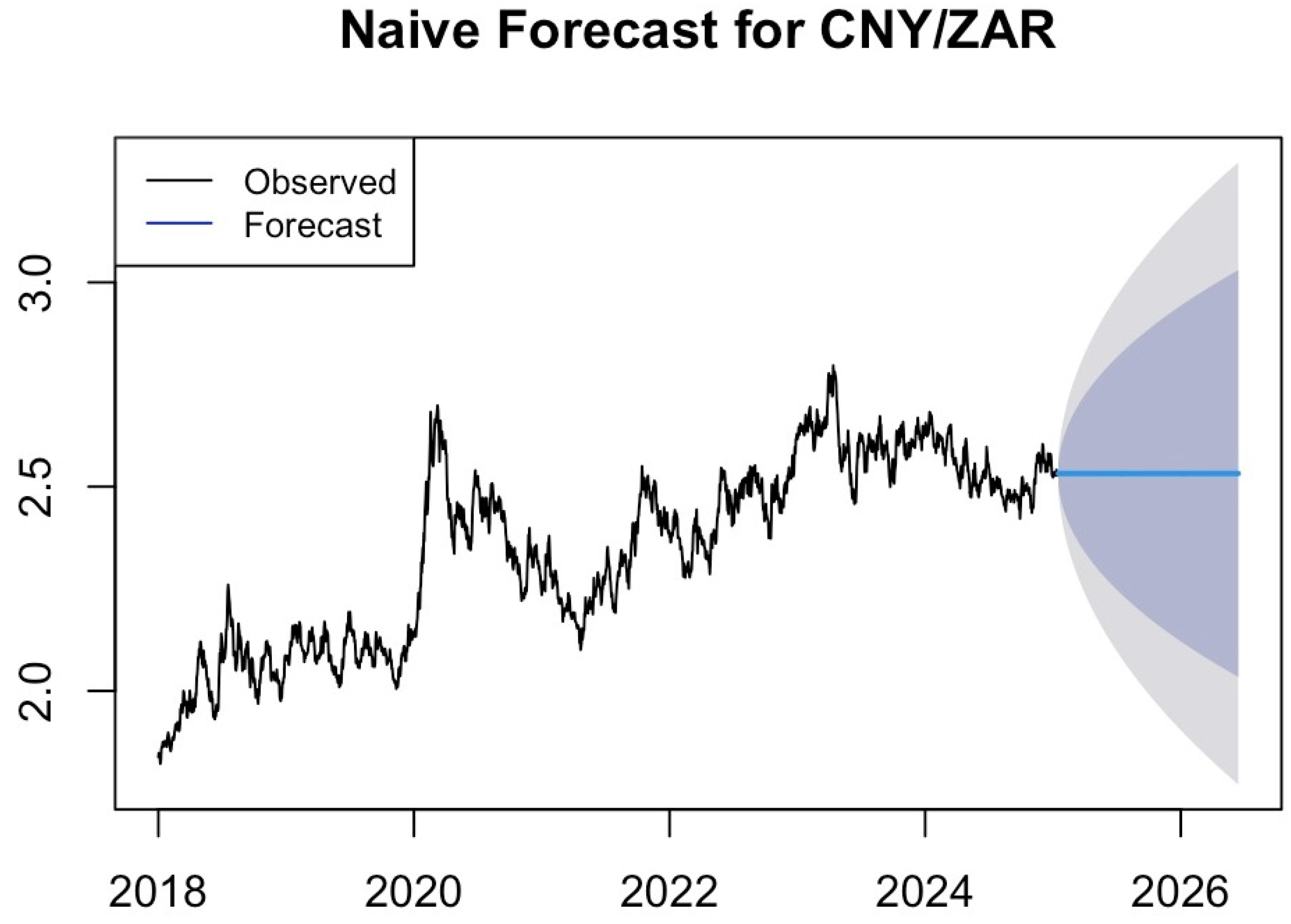
Figure 5 displays a naive random walk forecast for the EUR/ZAR exchange rate. The flat, horizontal point forecast line extending from the last observed value, accompanied by rapidly widening 80% and 95% prediction intervals, visually confirms that the naive model provides no meaningful directional guidance and fails to capture the dynamic, volatile nature of EUR/ZAR exchange rate movements over the forecast horizon. The naive forecast plots for the remaining three currency pairs, BRL/ZAR, CHF/ZAR, and CNY/ZAR, are shown in Appendix A and have broadly similar characteristics, confirming the inferiority of the naive random walk benchmark across all four exchange rate markets examined in this study.
Figure 5.
Naive random walk forecast for the EUR/ZAR exchange rate.
4. Discussion
4.1. General Discussion
This study examined the short-term performance of SVR when compared to PCR and XGBoost over four ZAR exchange rate markets of EUR/ZAR, CHF/ZAR, BRL/ZAR, and CNY/ZAR, using 80% and 95% training splits, with forecast accuracy evaluated using RMSE, MAE, and the Diebold–Mariano (DM) test. At the 80% training split, SVR-Linear outperforms PCR across all four currency pairs, with DM test statistics ranging from −2.88 to −3.84 (), confirming that these differences are statistically significant and reflect genuine improvements in predictive performance attributable to SVR’s superior ability to capture the nonlinear and nonstationary dynamics of emerging market exchange rate data that PCR’s linear framework cannot adequately model. This finding is robust to the choice of training split, as the 95% split produces consistent results with DM statistics ranging from −2.84 to −3.25 () across all four currency pairs, confirming that SVR-Linear’s statistical superiority over PCR is maintained regardless of the volume of training data used. Notably, despite PCR recording marginally lower point forecast errors than SVR-Linear for the CHF/ZAR pair at both splits, the DM test statistics of −3.77 () at the 80% split and −3.20 () at the 95% split consistently confirm SVR-Linear’s statistical superiority for this pair when the full distribution of forecast errors is considered over the complete test period, while SVR-Linear records lower point forecast errors than XGBoost across most pairs at both training splits, DM test statistics ranging from −0.57 to −1.01 ( to 0.571) at the 80% split and from −0.38 to −0.80 ( to 0.706) at the 95% split indicate that the two models are statistically equivalent in forecasting accuracy at both training configurations, suggesting that XGBoost’s additional ensemble complexity offers no statistically meaningful forecasting advantage over the more parsimonious SVR-Linear approach in the short-term ZAR exchange rate forecasting context.
4.2. Limitations of the Analysis
This study has several important limitations that should be considered when interpreting the findings. First, although this study employed two training splits of 80% and 95% to assess the robustness of the results, the use of only two fixed training and testing splits may still limit the reliability and generalisability of the accuracy measurements compared to more comprehensive cross-validation approaches such as rolling window or expanding window estimation, which are commonly employed in financial time series forecasting to simulate real-world forecasting conditions better. Second, we did not consider other useful approaches, such as random forests, LSTM networks, and hybrid models; only 3 forecasting models (support vector regression (SVR), XGBoost, and principal component regression (PCR)) were examined. This could influence the generalisability of the findings to other modelling frameworks. Third, hyperparameter tuning was restricted to SVR and XGBoost; a broader optimisation might have enhanced prediction performance. Fourth, given that the study was mainly conducted on exchange rate markets with varying levels of volatility, liquidity, and macroeconomic features (specific to EUR/ZAR, CHF/ZAR, BRL/ZAR, and CNY/ZAR), its conclusions may not be as generalisable to other currencies. Lastly, if XGBoost is not well regularised, it may overfit, leading to less interpretability. SVR and XGBoost both have well-accepted natural nonlinearities, though extreme outliers, kernel choice, and scaling can affect performance.
5. Conclusions
The research uses daily secondary data from Investing.com to forecast short-term changes in four South African Rand exchange rates, namely, EUR/ZAR, CHF/ZAR, BRL/ZAR, and CNY/ZAR, collected from 13 February 2018 to 24 February 2025. The proposed forecasting method—Support Vector Regression (SVR)—is compared with two other models: Principal Component Regression (PCR) and eXtreme Gradient Boosting (XGBoost). The accuracy of forecasts is assessed using the Root Mean Square Error (RMSE) and Mean Absolute Error (MAE) metrics, calculated for two sample splits: 80/20 and 95/5. SVR-Linear achieves the lowest RMSE and MAE for the EUR/ZAR, BRL/ZAR, and CNY/ZAR exchange rates, indicating its greater ability to accurately forecast changes in those rates.
Regarding the CHF/ZAR currency pair, PCR indicates a lower raw forecast error. However, it is important to note that Diebold–Mariano test results indicate that the forecast error distribution of SVR-Linear is statistically better than PCR’s during the entire test period. The difference between the two models is crucial for risk managers, as a better statistical distribution will affect VaR calculations and improve the effectiveness of hedging decisions during periods of market volatility. Finally, XGBoost performs fairly well, achieving the same accuracy as SVR-Linear in some cases, making it a possible choice depending on risk tolerance and computational resources.
Author Contributions
Conceptualisation, T.R., T.H.T. and C.S.; methodology, S.A.F.; software, S.A.F.; validation, S.A.F., T.R., T.H.T. and C.S.; formal analysis, S.A.F.; investigation, S.A.F., T.R. and C.S.; data curation, S.A.F.; writing—original draft preparation, S.A.F.; writing—review and editing, S.A.F., T.R., T.H.T. and C.S.; visualisation, S.A.F.; supervision, T.R., T.H.T. and C.S.; project administration, T.R. and C.S.; funding acquisition, S.A.F. All authors have read and agreed to the published version of the manuscript.
Funding
This research was funded by the 2025 NRF Honours Postgraduate Scholarship, grant number REF NO: PMDS240916269105.
Institutional Review Board Statement
Not applicable.
Informed Consent Statement
Not applicable.
Data Availability Statement
The data were obtained from, and are openly available on the Gold website: https://www.investing. com/commodities/gold-historical-data, the USD/ZAR exchange rate website: https://www.investing.com/currencies/usd-zar, the platinum website: https://www.investing.com/commodities/platinum-historical-data, and the oil price (Brent crude) website: https://www.investing.com//brent-crude-historical-data. (all accessed on 18 September 2025). The analytic data can be accessed on https://github.com/csigauke/-Short-term-forecasting-of-the-Euro-Rand-exchange-rate-using-support-vector-regression (accessed on 20 March 2026).
Acknowledgments
The support from the 2025 NRF Honours Postgraduate Scholarship is gratefully acknowledged. Opinions expressed and conclusions arrived at are those of the authors and are not necessarily to be attributed to the NRF. The authors also thank the anonymous reviewers for their insightful comments that helped improve this manuscript.
Conflicts of Interest
The authors declare no conflicts of interest. The funders had no role in the design of the study; in the collection, analyses, or interpretation of data; in the writing of the manuscript; or in the decision to publish the results.
Abbreviations
The following abbreviations are used in this manuscript:
| ANN | Artificial Neural Networks |
| BRL | Brazilian Real |
| CHF | Swiss Franc |
| CNY | Chinese Yuan |
| DM | Diebold–Mariano |
| GARCH | Generalised Autoregressive Conditional Heteroskedasticity |
| JSE | Johannesburg Stock Exchange |
| MAE | Mean Absolute Error |
| PCR | Principal Component Regression |
| PCA | Principal Component Analysis |
| PC | Principal Components |
| POCID | Prediction of Change in Direction |
| RBF | Radial Basis Function |
| RMSE | Root Mean Square Error |
| SVD | Singular Value Decomposition |
| SVM | Support Vector Machines |
| SVR | Support Vector Regression |
| USD | United States Dollar |
| XGBoost | eXtreme Gradient Boosting |
| ZAR | South African Rand |
Appendix A. Supplementary Plots
Figure A1.
Best for BRL.
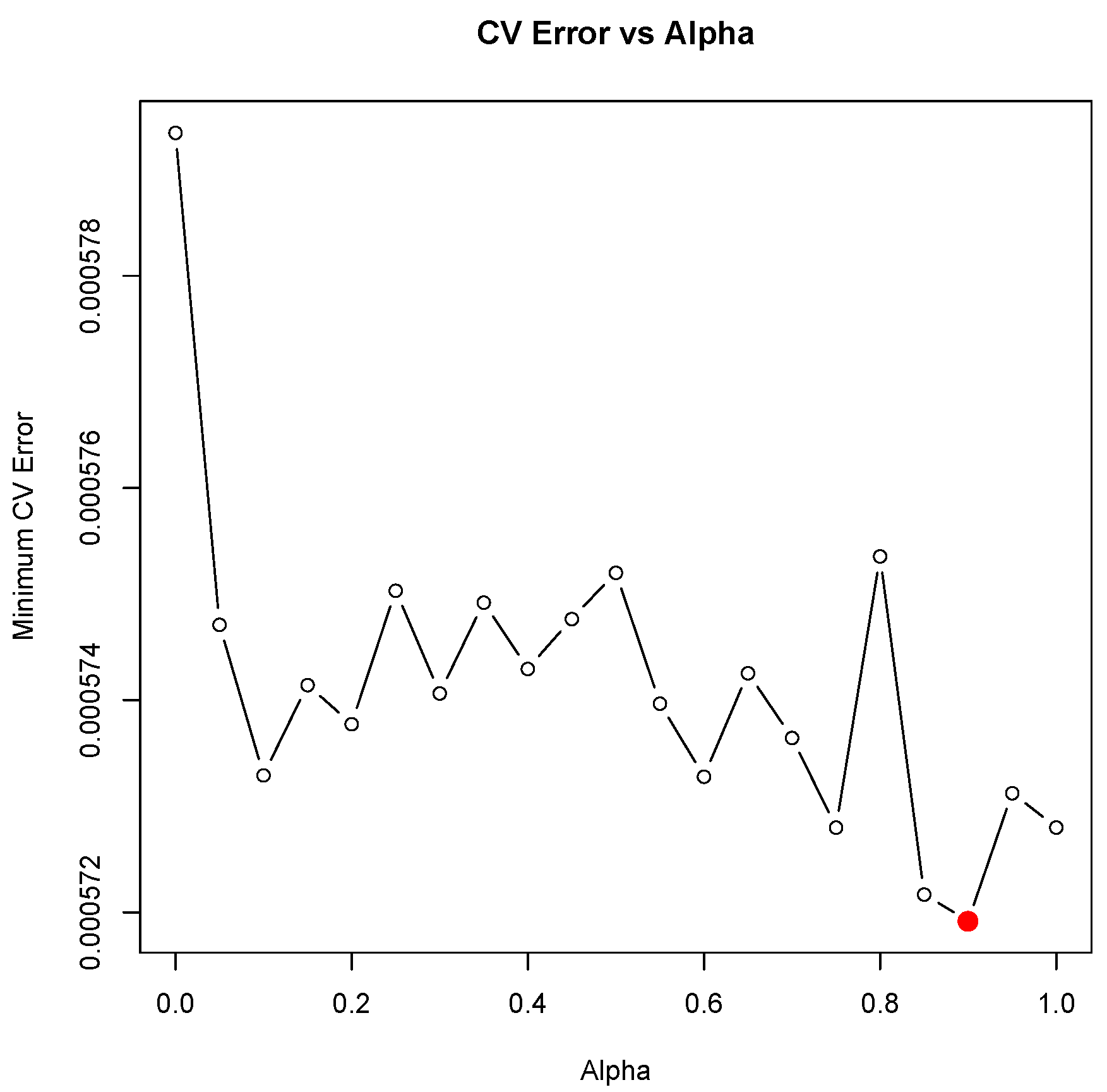
Figure A2.
Best for CHF.
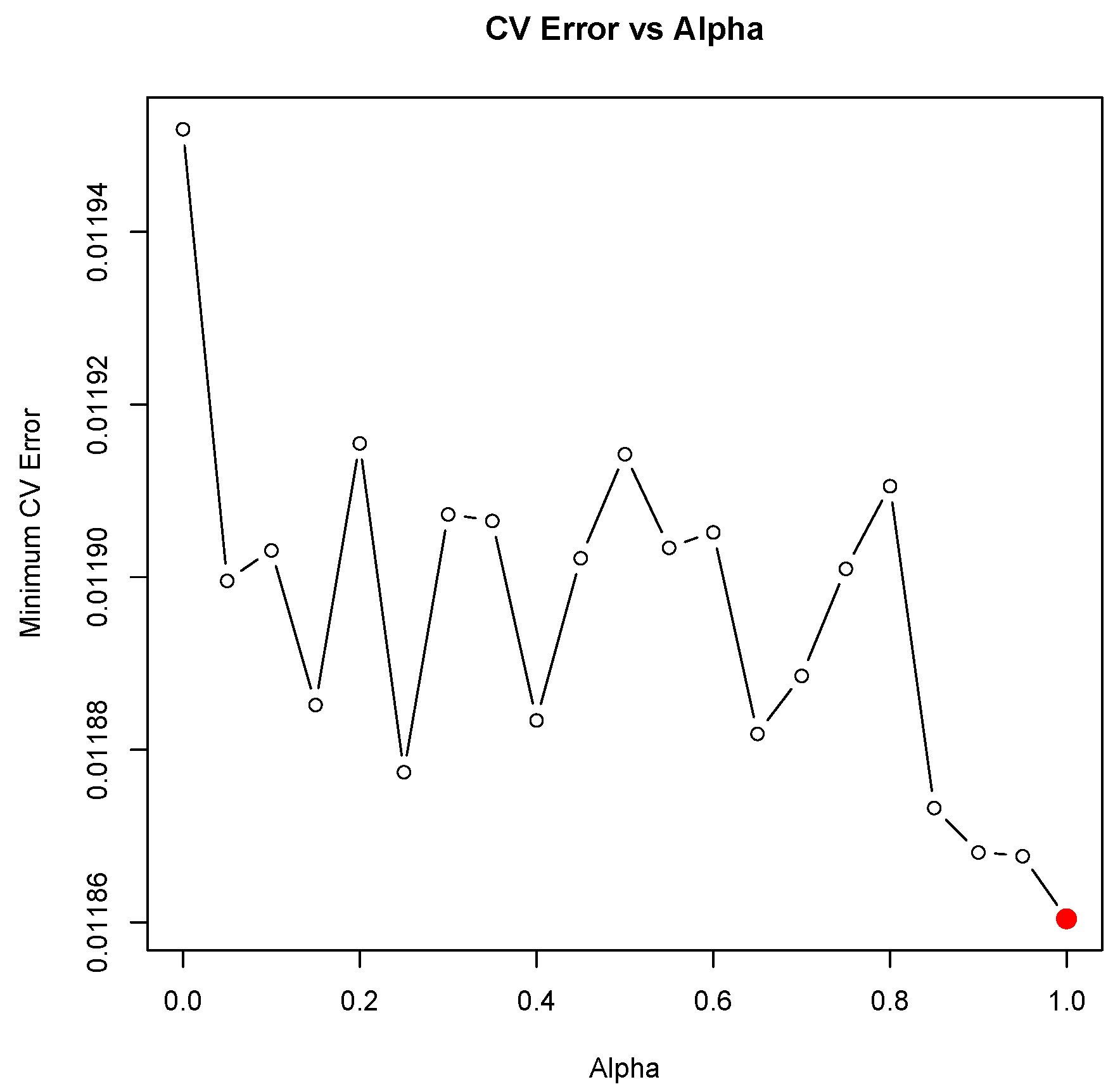
Figure A3.
Best CNY.
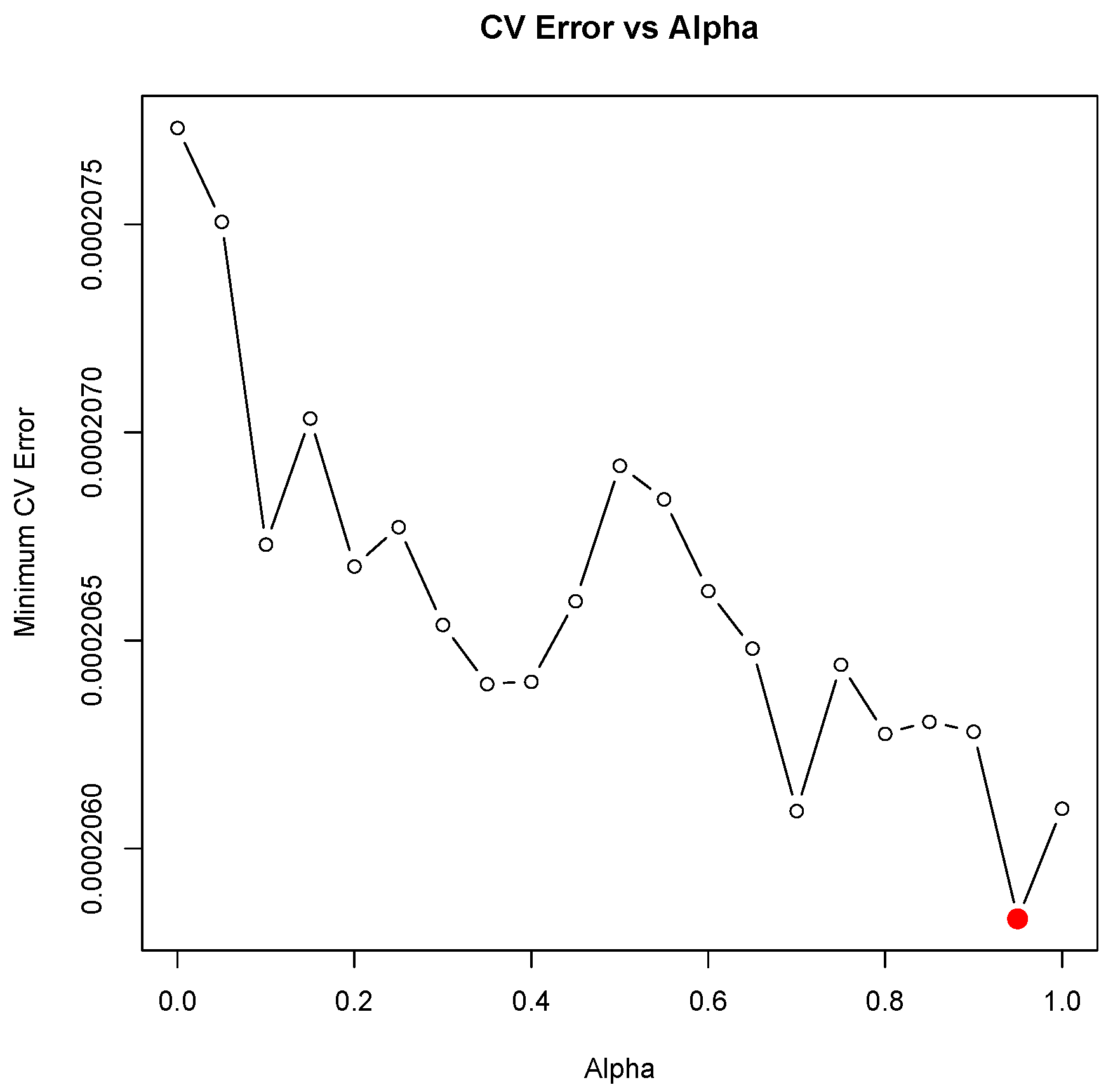
Figure A4.
Naive random walk forecast for the BRL/ZAR exchange rate.
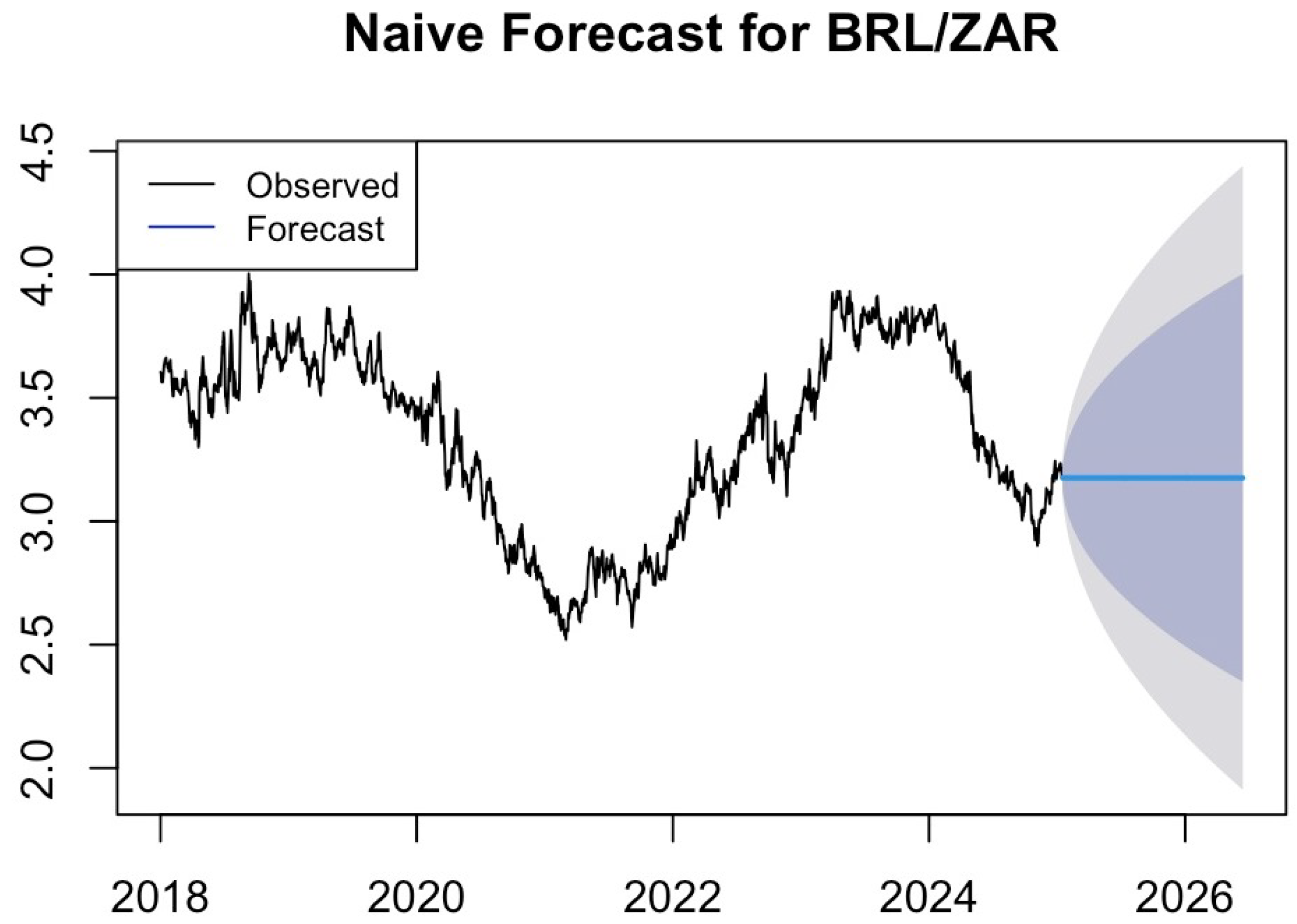
Figure A5.
Naive random walk forecast for the CHF/ZAR exchange rate.
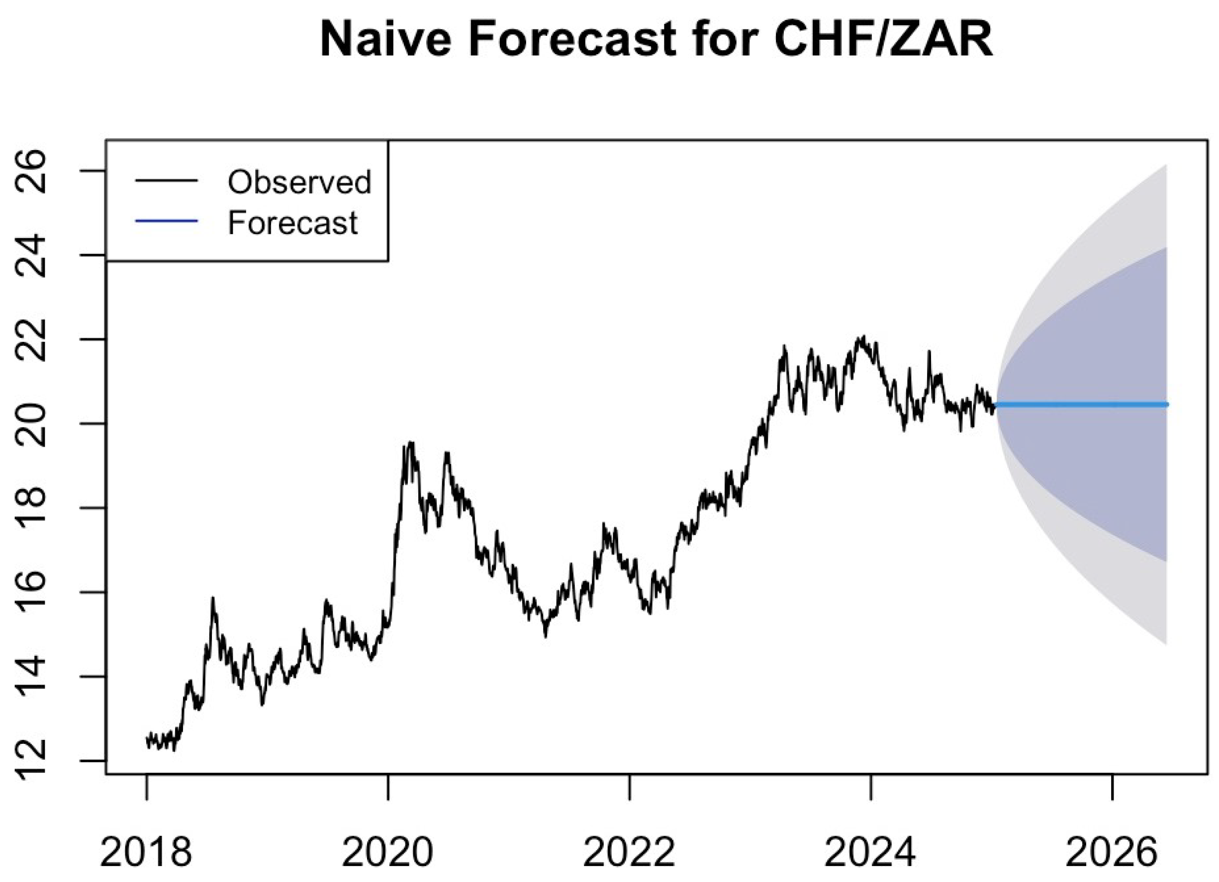
Figure A6.
Naive random walk forecast for the CNY/ZAR exchange rate.
References
- Abir, Shake Ibna, Sarder Abdulla Al Shiam, Rafi Muhammad Zakaria, Abid Hasan Shimanto, SM Shamsul Arefeen, Md Shah Ali Dolon, Nigar Sultana, and Shaharina Shoha. 2024. Use of AI-Powered Precision in Machine Learning Models for Real-Time Currency Exchange Rate Forecasting in BRICS Economies. Journal of Economics, Finance and Accounting Studies 6: 66–83. [Google Scholar] [CrossRef] [Scilit]
- Aydin, Zeliha Ergul, and Zehra Kamisli Ozturk. 2021. Performance Analysis of XGBoost Classifier with Missing Data. Manchester Journal of Artificial Intelligence and Applied Sciences 2: 2021. [Google Scholar]
- Bahramy, Farhad, and Sven F. Crone. 2013. Forecasting Foreign Exchange Rates Using Support Vector Regression. Paper presented at 2013 IEEE Conference on Computational Intelligence for Financial Engineering & Economics (CIFEr), New York, NY, USA, March 28–30; pp. 34–41. [Google Scholar]
- Bair, Eric, Trevor Hastie, Debashis Paul, and Robert Tibshirani. 2006. Prediction by Supervised Principal Components. Journal of the American Statistical Association 101: 119–37. [Google Scholar] [CrossRef] [Scilit]
- Cao, Ding-Zhou, Su-Lin Pang, and Yuan-Huai Bai. 2005. Forecasting Exchange Rate Using Support Vector Machines. Paper presented at 2005 International Conference on Machine Learning and Cybernetics, Guangzhou, China, August 18–21, vol. 6, pp. 3448–52. [Google Scholar]
- Chaudhary, Rashmi, Priti Bakhshi, and Hemendra Gupta. 2020. Volatility in International Stock Markets: An Empirical Study during COVID-19. Journal of Risk and Financial Management 13: 208. [Google Scholar] [CrossRef] [Scilit]
- Chen, Tianqi, and Carlos Guestrin. 2016. XGBoost: A Scalable Tree Boosting System. Paper presented at 22nd ACM SIGKDD International Conference on Knowledge Discovery and Data Mining, San Francisco, CA, USA, August 13–17; pp. 785–94. [Google Scholar]
- Cheung, Yin-Wong, Menzie D. Chinn, and Antonio Garcia Pascual. 2005. Empirical Exchange Rate Models of the Nineties: Are Any Fit to Survive? Journal of International Money and Finance 24: 1150–75. [Google Scholar] [CrossRef] [Scilit]
- Choudhry, Taufiq, Frank McGroarty, Ke Peng, and Shiyun Wang. 2012. High-Frequency Exchange-Rate Prediction with an Artificial Neural Network. Intelligent Systems in Accounting, Finance and Management 19: 170–78. [Google Scholar] [CrossRef] [Scilit]
- Devos, Olivier, Cyril Ruckebusch, Alexandra Durand, Ludovic Duponchel, and Jean-Pierre Huvenne. 2009. Support Vector Machines (SVM) in Near Infrared (NIR) Spectroscopy: Focus on Parameters Optimization and Model Interpretation. Chemometrics and Intelligent Laboratory Systems 96: 27–33. [Google Scholar] [CrossRef] [Scilit]
- Diebold, Francis X., and Robert S. Mariano. 2002. Comparing Predictive Accuracy. Journal of Business & Economic Statistics 20: 134–44. [Google Scholar] [CrossRef] [Scilit]
- Fallahtafti, Alireza, Mohammadreza Aghaaminiha, Sara Akbarghanadian, and Gary R. Weckman. 2022. Forecasting ATM Cash Demand Before and During the COVID-19 Pandemic Using an Extensive Evaluation of Statistical and Machine Learning Models. SN Computer Science 3: 164. [Google Scholar] [CrossRef] [Scilit]
- Ge, Jiankun, Linfeng Zhao, Zihui Yu, Huanhuan Liu, Lei Zhang, Xuewen Gong, and Huaiwei Sun. 2022. Prediction of Greenhouse Tomato Crop Evapotranspiration Using XGBoost Machine Learning Model. Plants 11: 1923. [Google Scholar] [CrossRef] [Scilit]
- He, Haibo, and Xiaoping Shen. 2007. Bootstrap Methods for Foreign Currency Exchange Rates Prediction. Paper presented at 2007 International Joint Conference on Neural Networks, Orlando, FL, USA, August 12–17; pp. 1272–77. [Google Scholar]
- Ibekwe, Uche Amaraa, and Abass A. Shiro. 2022. Modelling the Determinants of Naira/US Dollar Currency Exchange Rates Using Principal Component Analysis (PCA) and Singular Value Decomposition (SVD). Nigerian Journal of Risk and Insurance 12: 77–97. [Google Scholar]
- Ince, Huseyin, and Theodore B. Trafalis. 2006. A Hybrid Model for Exchange Rate Prediction. Decision Support Systems 42: 1054–62. [Google Scholar] [CrossRef] [Scilit]
- Jolliffe, Ian T. 2002. Choosing a Subset of Principal Components or Variables. In Principal Component Analysis. New York: Springer, pp. 92–114. [Google Scholar]
- Jolliffe, Ian T., and Jorge Cadima. 2016. Principal Component Analysis: A Review and Recent Developments. Philosophical Transactions of the Royal Society A: Mathematical, Physical and Engineering Sciences 374: 20150202. [Google Scholar] [CrossRef] [Scilit] [PubMed]
- Kamruzzaman, Joarder, Ruhul A. Sarker, and Iftekhar Ahmad. 2003. SVM Based Models for Predicting Foreign Currency Exchange Rates. In Third IEEE International Conference on Data Mining, Melbourne, FL, USA, November 19–22. New York: IEEE, pp. 557–60. [Google Scholar]
- Karatzoglou, Alexandros, David Meyer, and Kurt Hornik. 2006. Support vector machines in R. Journal of Statistical Software 15: 1–28. [Google Scholar] [CrossRef] [Scilit]
- Karunasingha, Dulakshi Santhusitha Kumari. 2022. Root Mean Square Error or Mean Absolute Error? Use Their Ratio as Well. Information Sciences 585: 609–29. [Google Scholar] [CrossRef] [Scilit]
- Kerschen, Gaëtan, and J.-C. Golinval. 2002. Non-Linear Generalization of Principal Component Analysis: From a Global to a Local Approach. Journal of Sound and Vibration 254: 867–76. [Google Scholar] [CrossRef] [Scilit]
- Kim, Hyun-jung, and Kyung-shik Shin. 2007. A Hybrid Approach Based on Neural Networks and Genetic Algorithms for Detecting Temporal Patterns in Stock Markets. Applied Soft Computing 7: 569–76. [Google Scholar] [CrossRef] [Scilit]
- Kim, Kwang In, Keechul Jung, Se Hyun Park, and Hang Joon Kim. 2002. Support Vector Machines for Texture Classification. IEEE Transactions on Pattern Analysis and Machine Intelligence 24: 1542–50. [Google Scholar] [CrossRef] [Scilit]
- Liu, R. X., J. Kuang, Qiong Gong, and X. L. Hou. 2003. Principal Component Regression Analysis with SPSS. Computer Methods and Programs in Biomedicine 71: 141–47. [Google Scholar] [CrossRef] [Scilit]
- Lothian, James R. 2001. Exchange Rates. In Oxford Encyclopedia of Economic History. Oxford: Oxford University Press. [Google Scholar]
- Lu, Chi-Jie, Tian-Shyug Lee, and Chih-Chou Chiu. 2009. Financial Time Series Forecasting Using Independent Component Analysis and Support Vector Regression. Decision Support Systems 47: 115–25. [Google Scholar] [CrossRef] [Scilit]
- Mark, Nelson C. 1995. Exchange Rates and Fundamentals: Evidence on Long-Horizon Predictability. The American Economic Review 85: 201–18. [Google Scholar]
- Meese, Richard A., and Kenneth Rogoff. 1983. Empirical Exchange Rate Models of the Seventies: Do They Fit Out of Sample? Journal of International Economics 14: 3–24. [Google Scholar] [CrossRef] [Scilit]
- Mevik, Bjørn-Helge, and Ron Wehrens. 2015. Introduction to the Pls Package. Help Section of the “Pls” Package of R Studio Software 1: 1–23. [Google Scholar]
- Moosa, Imad A. 2016. Exchange Rate Forecasting: Techniques and Applications. Berlin and Heidelberg: Springer. [Google Scholar]
- Ndlovu, Xolani, and Eric Schaling. 2018. The South African Rand, Fundamentals and Commodity Prices. African Review of Economics and Finance 10: 23–31. [Google Scholar]
- Panda, Chakradhara, and V. Narasimhan. 2007. Forecasting Exchange Rate Better with Artificial Neural Network. Journal of Policy Modeling 29: 227–36. [Google Scholar] [CrossRef] [Scilit]
- Plasmans, Joseph, William Verkooijen, and Hennie Daniels. 1998. Estimating Structural Exchange Rate Models by Artificial Neural Networks. Applied Financial Economics 8: 541–51. [Google Scholar] [CrossRef] [Scilit]
- Ponomareva, Natalia, Jeffrey Sheen, and Ben Zhe Wang. 2019. Forecasting Exchange Rates Using Principal Components. Journal of International Financial Markets, Institutions and Money 63: 101131. [Google Scholar] [CrossRef] [Scilit]
- Potgieter, Janette. 2005. Fundamentals of the Rand/Euro Exchange Rate: A Behavioural Approach. Ph.D. thesis, North West University, North West, South Africa. [Google Scholar]
- Raudys, Aistis, and Edvinas Goldstein. 2022. Forecasting Detrended Volatility Risk and Financial Price Series Using LSTM Neural Networks and XGBoost Regressor. Journal of Risk and Financial Management 15: 602. [Google Scholar] [CrossRef] [Scilit]
- Ryan, Janine. 2023. Understanding Why the Rand is Bleeding. Farmer’s Weekly 2023: 4. [Google Scholar]
- Shoko, Claris, and Caston Sigauke. 2023. Short-Term Forecasting of COVID-19 Using Support Vector Regression: An Application Using Zimbabwean Data. American Journal of Infection Control 51: 1095–107. [Google Scholar] [CrossRef] [Scilit]
- Smola, Alex J., and Bernhard Schölkopf. 2004. A Tutorial on Support Vector Regression. Statistics and Computing 14: 199–222. [Google Scholar] [CrossRef] [Scilit]
- Tay, Francis E. H., and Lijuan Cao. 2001. Application of Support Vector Machines in Financial Time Series Forecasting. Omega 29: 309–17. [Google Scholar] [CrossRef] [Scilit]
- Tharwat, Alaa. 2019. Parameter Investigation of Support Vector Machine Classifier with Kernel Functions. Knowledge and Information Systems 61: 1269–302. [Google Scholar] [CrossRef] [Scilit]
- Tibshirani, Robert J. 2014. Lasso and Sparsity in Statistics. Statistics in Action: A Canadian Outlook 79: 14. [Google Scholar]
- Triacca, U. 2018. Comparing Predictive Accuracy of Two Forecasts. Available online: https://www.lem.sssup.it/phd/documents/Lesson19.pdf (accessed on 18 September 2025).
- Vapnik, Vladimir. 2013. The Nature of Statistical Learning Theory. Berlin and Heidelberg: Springer. [Google Scholar]
- Vapnik, Vladimir N. 1998. The Nature of Statistical Learning Theory. Berlin and Heidelberg: Springer. [Google Scholar]
- Vapnik, Vladimir N. 1999. An Overview of Statistical Learning Theory. IEEE Transactions on Neural Networks 10: 988–99. [Google Scholar] [CrossRef] [Scilit]
- Vlok, Cassius Ray. 2024. On Retraining Intervals and Sequence Lengths for Machine Learning Models in Foreign Exchange Rate Forecasting. Ph.D. dissertation, Stellenbosch University, Stellenbosch, South Africa. [Google Scholar]
- Wang, You-Gan, Jinran Wu, Zhi-Hua Hu, and Geoffrey J. McLachlan. 2023. A New Algorithm for Support Vector Regression with Automatic Selection of Hyperparameters. Pattern Recognition 133: 108989. [Google Scholar] [CrossRef] [Scilit]
- Yaohao, Peng, and Pedro Henrique Melo Albuquerque. 2019. Non-Linear Interactions and Exchange Rate Prediction. Applied Mathematical Finance 26: 69–100. [Google Scholar] [CrossRef] [Scilit]
- Zhang, Guoqiang Peter, and Victor L. Berardi. 2001. Time Series Forecasting with Neural Network Ensembles. Journal of the Operational Research Society 52: 652–64. [Google Scholar] [CrossRef] [Scilit]
- Zheng, Jing, Xiao Fu, and Guijun Zhang. 2019. Research on Exchange Rate Forecasting Based on Deep Belief Network. Neural Computing and Applications 31: 573–82. [Google Scholar] [CrossRef] [Scilit]
- Zhu, Yiming. 2023. Stock Price Prediction Based on LSTM and XGBoost Combination Model. Transactions on Computer Science and Intelligent Systems Research 1: 94–109. [Google Scholar] [CrossRef] [Scilit]
- Zou, Hui, and Trevor Hastie. 2005. Regularization and Variable Selection via the Elastic Net. Journal of the Royal Statistical Society Series B: Statistical Methodology 67: 301–20. [Google Scholar] [CrossRef] [Scilit]
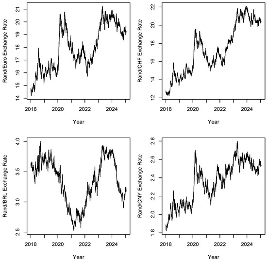
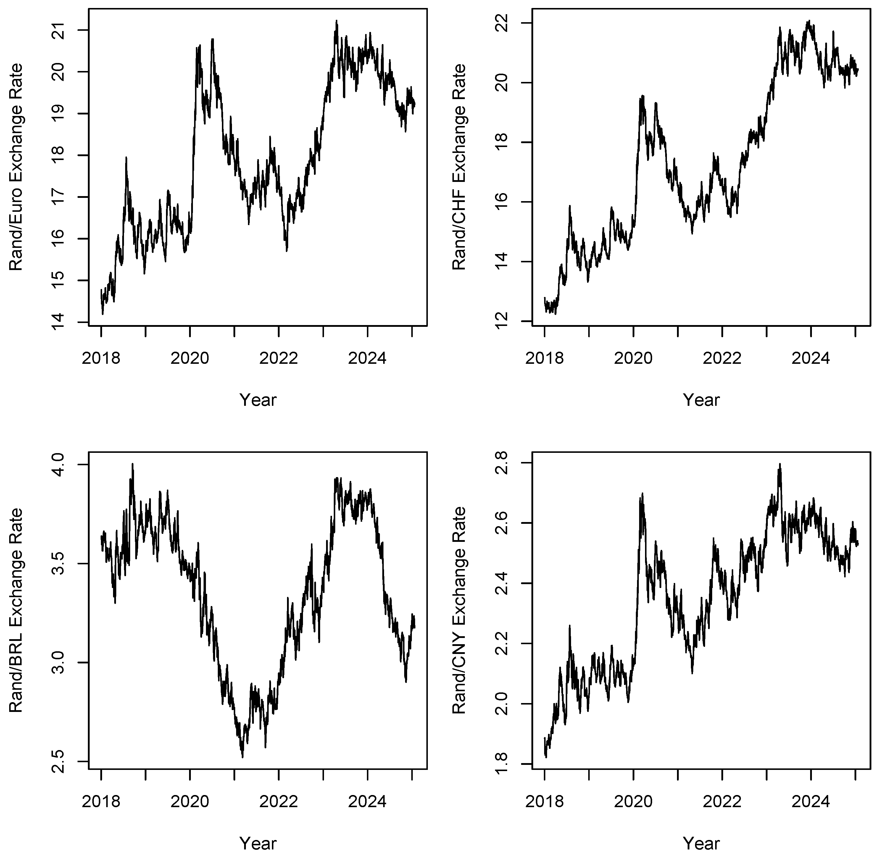
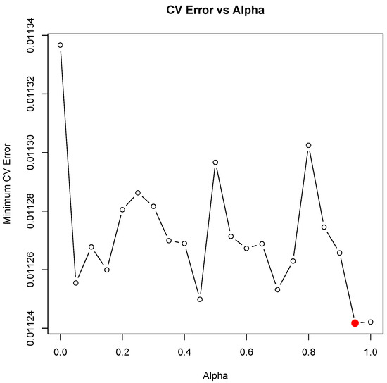
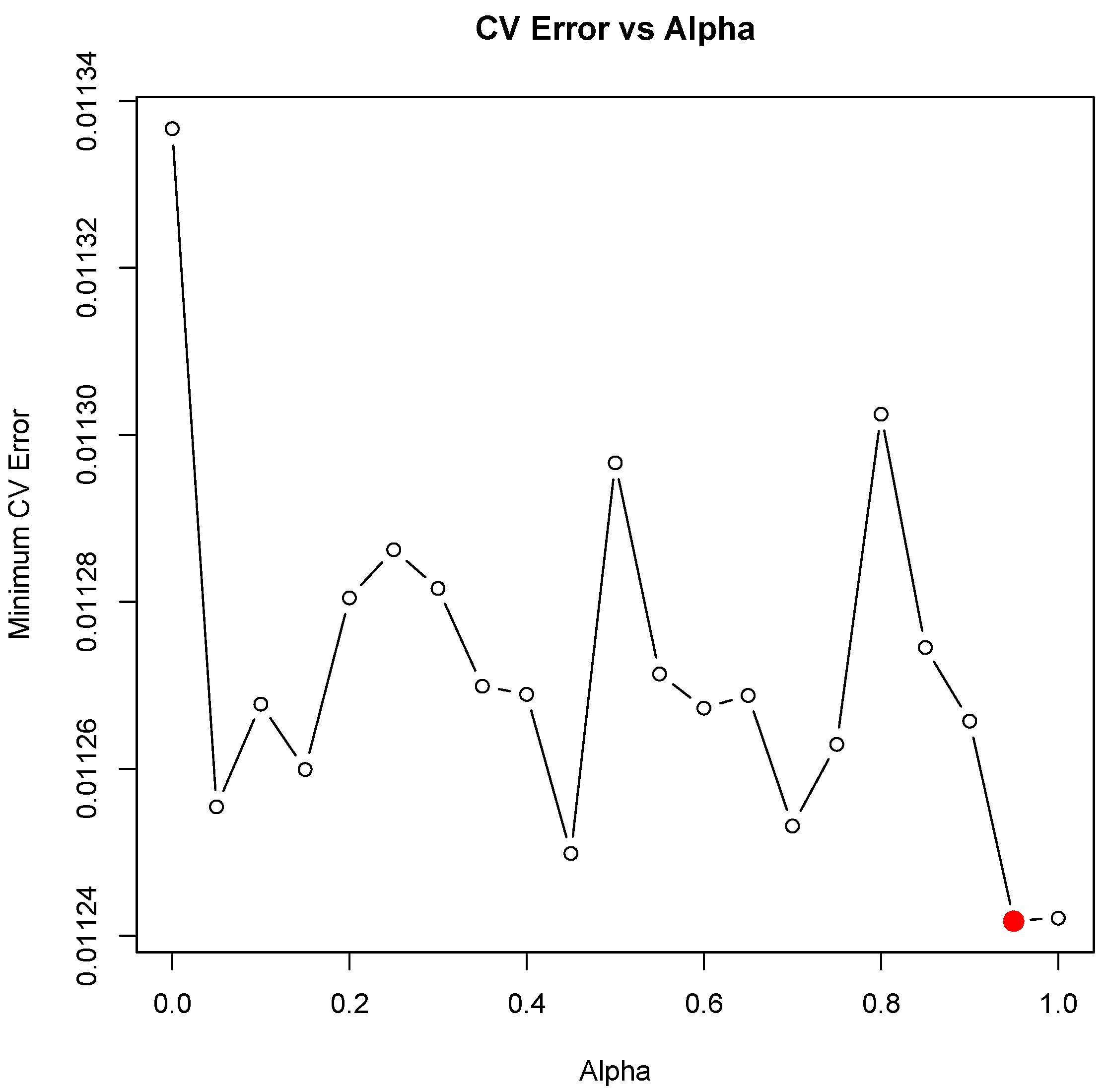
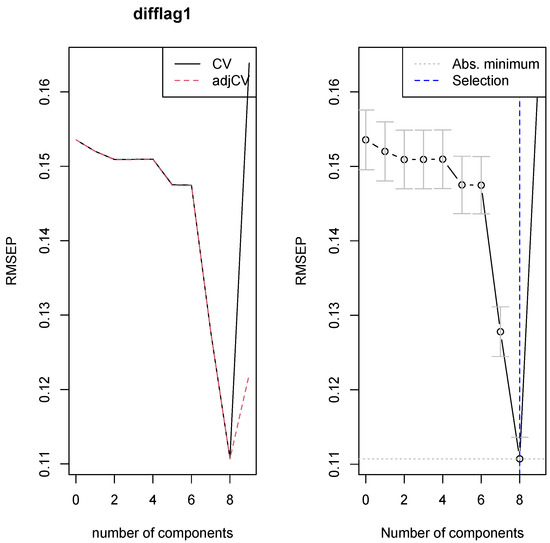
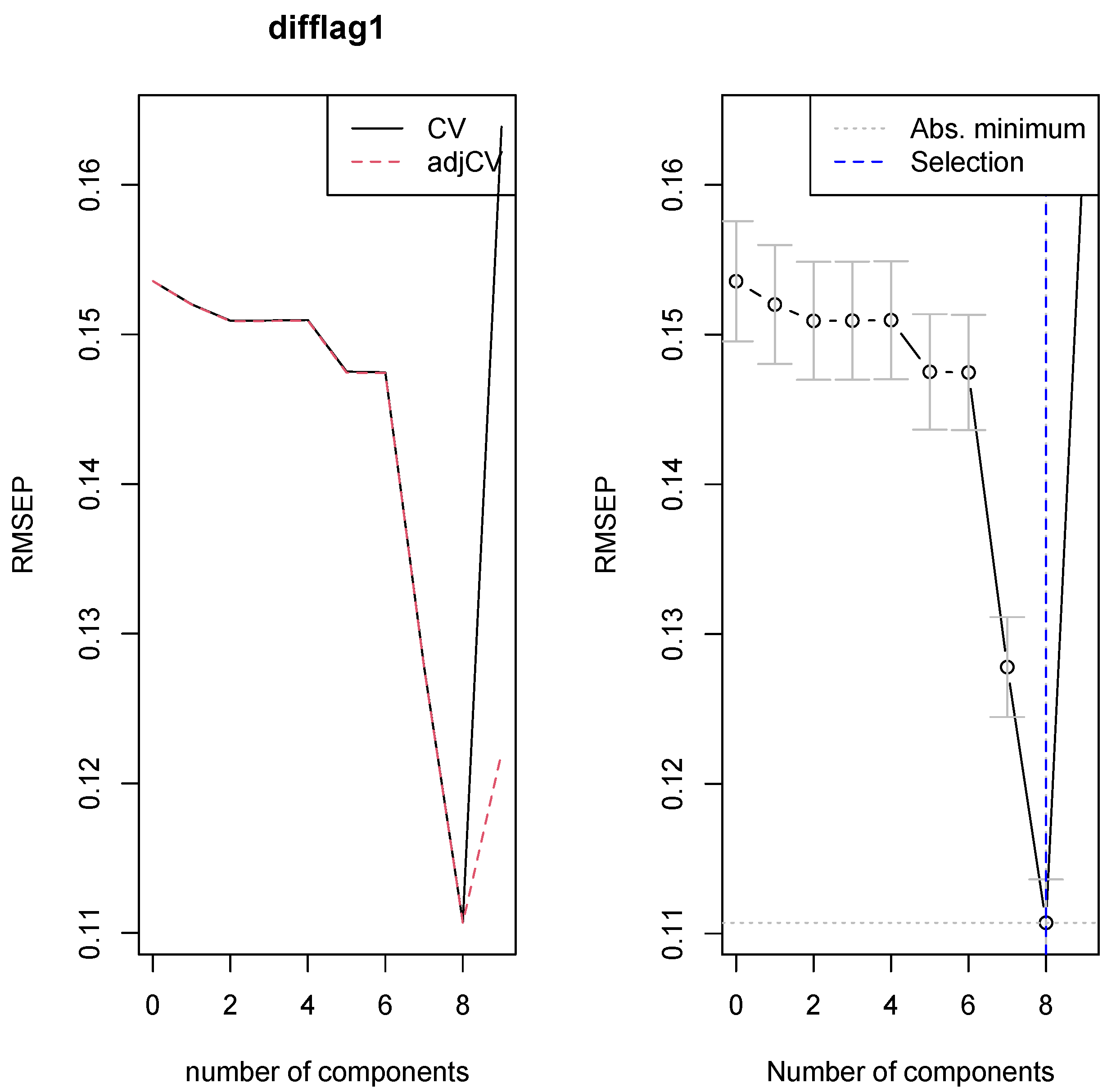
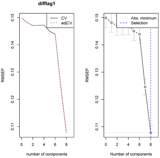
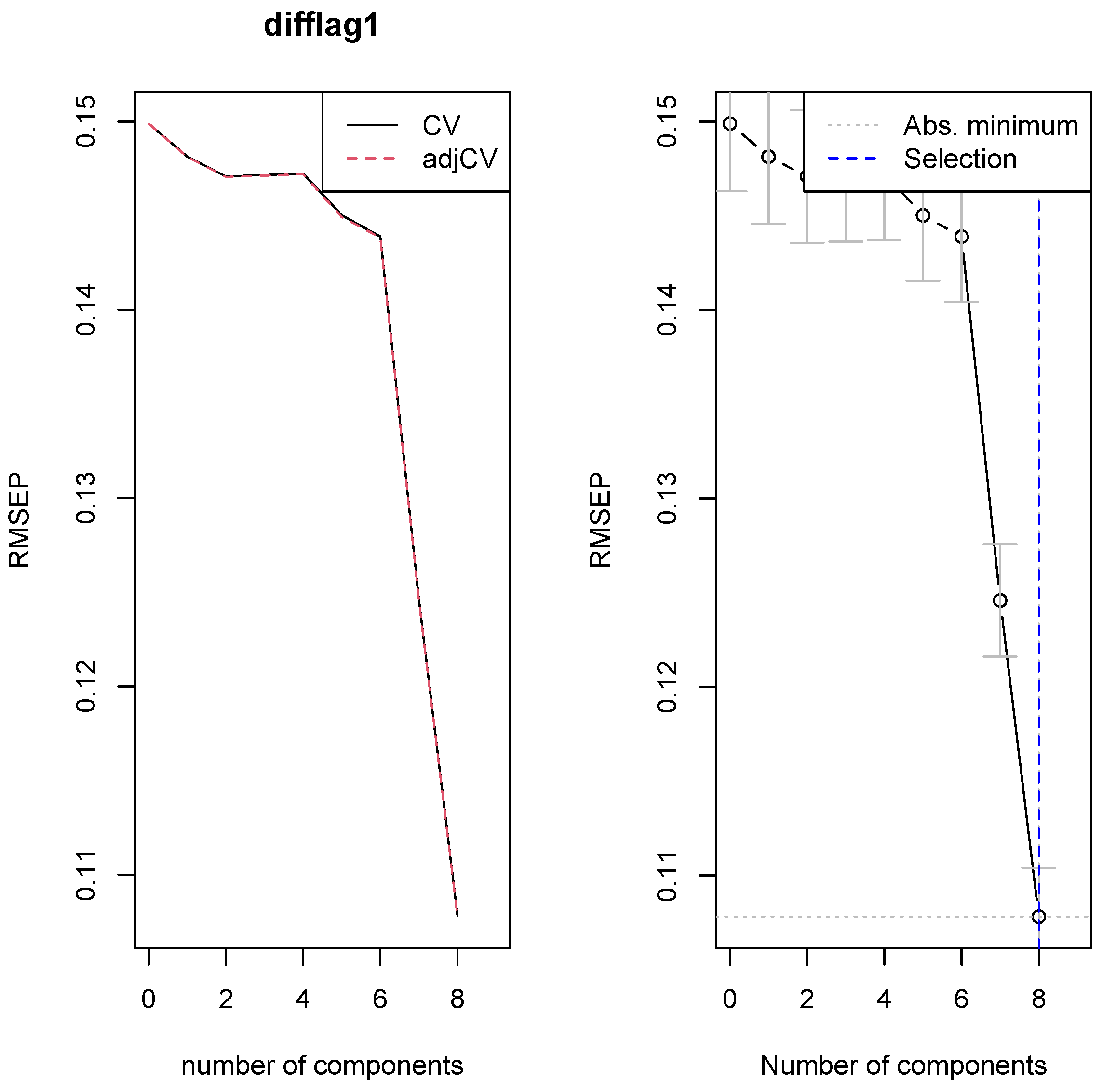
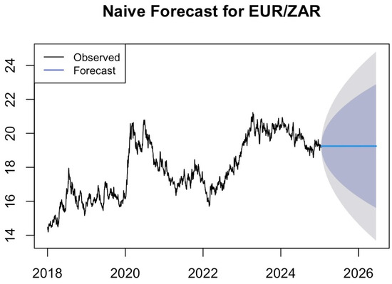
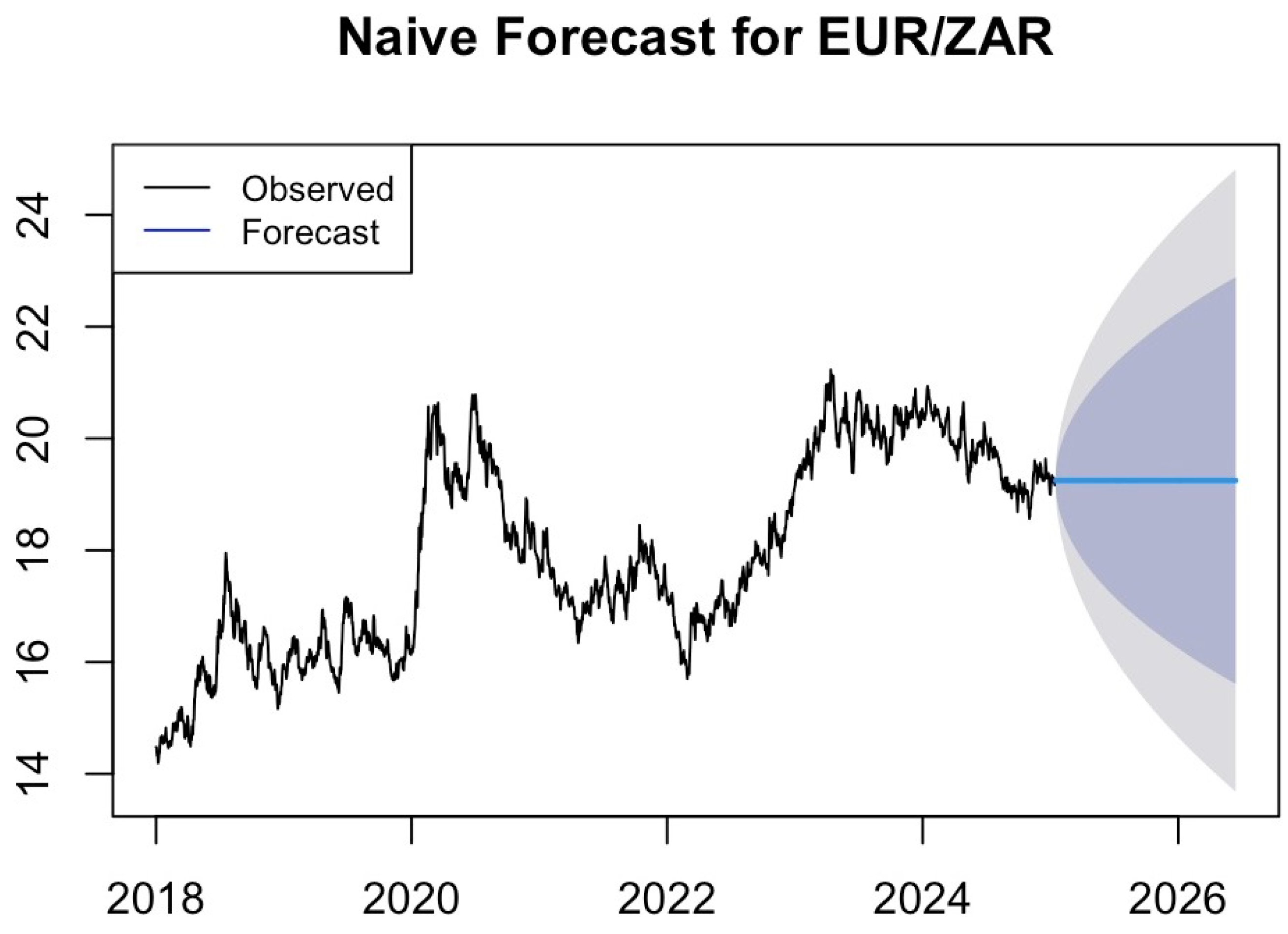

Disclaimer/Publisher’s Note: The statements, opinions and data contained in all publications are solely those of the individual author(s) and contributor(s) and not of MDPI and/or the editor(s). MDPI and/or the editor(s) disclaim responsibility for any injury to people or property resulting from any ideas, methods, instructions or products referred to in the content. |
© 2026 by the authors. Licensee MDPI, Basel, Switzerland. This article is an open access article distributed under the terms and conditions of the Creative Commons Attribution (CC BY) license.