


Abstract
Cryptocurrency markets combine persistent volatility, heavy tails, and recurrent stress episodes. This study asks whether portfolio optimization is sufficient to manage these risks for Bitcoin, Ethereum, Binance Coin, Solana, and XRP, using 1454 daily observations from January 2022 to January 2026. Student-t GARCH and DCC-GARCH forecasts feed static and rolling allocation rules, evaluated out of sample and net of transaction costs against equal-weight, minimum-variance, risk-parity, and minimum-CVaR benchmarks; downside risk is backtested with Kupiec and Christoffersen tests, and three anomaly detectors are validated against four crisis windows, including expanding-window refits. Volatility persistence ranges from 0.912 to 1.000, and average conditional correlations are higher inside four crisis windows than outside (0.76 vs. 0.66), a contrast that exceeds placebo windows but is small relative to neighbouring days. In sample, maximum-Sharpe weights raise the Sharpe ratio (0.88 vs. 0.76) without statistical significance; out of sample, their point estimate is lower than that of equal weighting (0.92 vs. 1.15), a difference that is statistically inconclusive. Risk-based rules cut volatility by about 19% and maximum drawdown by 10 points, whereas GARCH–DCC allocation adds turnover without further gains, and minimum-CVaR cannot be distinguished from minimum-variance allocation in this sample, the tests having limited power. Isolation Forest flags are about 8 times more concentrated in crisis windows than chance, and about 10 times when refitted on an expanding window. Optimization lowers risk, whereas evidence that it improves risk-adjusted performance is inconclusive.
1. Introduction
The increasing institutionalization of cryptocurrency markets has transformed digital assets from speculative instruments into increasingly relevant components of diversified investment portfolios. Bitcoin, Ethereum, Binance Coin, Solana, and XRP now attract substantial attention from both institutional and retail investors. Yet, the repeated occurrence of major market disruptions, including the COVID-19 market collapse, the Terra/Luna crisis, and the failure of FTX, has highlighted the fragility of cryptocurrency markets and renewed concerns regarding volatility, tail risk, and portfolio resilience.
This evolution raises a fundamental question for investment management: can portfolio optimization alone provide adequate protection against the extreme volatility and downside risk that characterize digital assets, or should it be complemented by volatility forecasting and anomaly-detection mechanisms? While cryptocurrencies offer important return opportunities, their return distributions differ markedly from those observed in traditional asset classes. High volatility, volatility clustering, heavy tails, and abrupt reversals challenge conventional allocation frameworks and complicate risk-management decisions.
The foundations of portfolio allocation originate from the seminal work on mean–variance portfolio selection (Markowitz 1952). However, the effectiveness of the mean-variance framework depends critically on how risk is measured and anticipated. In cryptocurrency markets, risk assessment is particularly challenging because return dynamics often violate assumptions commonly adopted in traditional financial modelling. Consequently, investors increasingly require complementary approaches capable of capturing both conditional volatility and exposure to extreme losses (Rockafellar and Uryasev 2000).
Conditional volatility modelling has become a central element of cryptocurrency risk analysis. Following the foundational contributions on conditional heteroskedasticity (Engle 1982; Bollerslev 1986), GARCH-type models have become standard tools for modelling time-varying risk. Empirical evidence consistently documents strong volatility persistence and clustering effects in cryptocurrency returns (Dyhrberg 2016; Chu et al. 2017; Katsiampa 2017; Baur and Dimpfl 2018). At the same time, studies on cryptocurrency portfolio allocation indicate that investment performance may improve when return, volatility, and dependence structures are jointly considered (Platanakis and Urquhart 2019, 2020).
Despite these advances, the literature remains fragmented. Existing studies have generally examined volatility modelling, portfolio optimization, downside-risk assessment, and anomaly detection as separate research streams. Limited evidence is available regarding the extent to which these dimensions interact and jointly contribute to portfolio resilience. This issue is particularly relevant because extreme events may simultaneously affect volatility, diversification benefits, and downside risk.
The objective of this study is to evaluate whether the integration of volatility modelling, portfolio optimization, downside-risk assessment, and anomaly-detection techniques can improve risk-adjusted portfolio performance. Particular attention is devoted to the interaction between volatility persistence, tail risk, and abnormal market conditions, three characteristics that have become increasingly relevant as cryptocurrency markets mature and attract broader investor participation.
The empirical analysis is guided by four expectations derived from the literature. Cryptocurrency returns are expected to exhibit persistent conditional volatility; optimized portfolios are expected to generate superior risk-adjusted performance relative to naïve allocations; downside-risk measures are expected to provide information beyond conventional volatility indicators; and anomaly-detection procedures are expected to improve the identification of abnormal market conditions.
To investigate these issues, the study combines descriptive analysis, Student-t GARCH and DCC-GARCH modelling, static and rolling portfolio optimization, tail-risk measurement, and anomaly detection within a unified empirical framework in which volatility and correlation forecasts feed directly into the allocation rules. The robustness of the findings is assessed through complementary procedures, including KPSS testing, ARCH-LM diagnostics, Ljung–Box tests, asymmetric GARCH specifications, rolling out-of-sample evaluation net of transaction costs, Kupiec and Christoffersen backtesting, block-bootstrap inference, and a sensitivity analysis of the anomaly detectors.
The contribution of this article is threefold. First, it provides an integrated framework in which GARCH–DCC covariance forecasts are used as inputs to the allocation, so that volatility modelling, portfolio construction, downside-risk assessment, and anomaly detection are linked rather than run in parallel. Second, it evaluates static and dynamic allocation rules out of sample and net of transaction costs against risk-based benchmarks (minimum variance, risk parity, and minimum CVaR), and finds that the benefit of optimization that can be demonstrated in cryptocurrency markets lies in risk reduction, whereas the evidence on the Sharpe ratio is inconclusive given the width of the confidence intervals. Third, it validates three anomaly detectors against crisis windows defined independently of the detection output, using precision, recall, enrichment, threshold-free discrimination, and detection delay, and tests their robustness to look-ahead and circularity by refitting them on an expanding window and by applying the Isolation Forest to volatility-standardized returns. A methodological contribution is the documentation of a timestamp-synchronization step and of an out-of-sample risk-forecasting design that prevent spurious diversification and tautological in-sample VaR backtests.
The remainder of the paper is organized as follows. Section 2 reviews the relevant literature. Section 3 presents the data and methodology. Section 4 reports the empirical findings. Section 5 discusses the results and their implications for investors and risk managers. Finally, Section 6 concludes and outlines directions for future research.
2. Literature Review
2.1. Cryptocurrencies as an Emerging Asset Class
Whether cryptocurrencies should be regarded as a distinct asset class remains an important question in the asset-pricing literature. Their growing institutional adoption and increasing integration into investment portfolios suggest that they have moved beyond their original role as speculative digital instruments. At the same time, their economic characteristics continue to differ substantially from those of traditional financial assets. Unlike equities, cryptocurrencies do not generate cash flows, while unlike sovereign securities, they do not benefit from explicit guarantees or monetary support mechanisms.
Existing evidence indicates that cryptocurrency returns are largely driven by market-specific factors rather than conventional macroeconomic determinants (Liu and Tsyvinski 2021). This observation has important implications for portfolio management because assets driven by independent risk factors may provide diversification benefits even when their volatility remains elevated. However, the economic relevance of cryptocurrencies as a portfolio component continues to be debated given their limited fundamental anchors, high sensitivity to investor sentiment, and exposure to extreme market events.
From an investment perspective, the key issue is therefore not whether cryptocurrencies generate high returns, but whether these returns compensate investors for the substantial risks they bear. This perspective shifts the focus from pure performance analysis to the broader question of portfolio efficiency and risk-adjusted investment outcomes.
2.2. Portfolio Optimization and Cryptocurrency Investment
The relationship between cryptocurrencies and portfolio efficiency has attracted growing attention in recent years. Building upon the mean–variance paradigm (Markowitz 1952), researchers have investigated whether cryptocurrencies improve portfolio performance once risk is explicitly incorporated into the allocation process.
Empirical findings are mixed. Some studies report that the inclusion of cryptocurrencies enhances the risk–return trade-off of diversified portfolios (Platanakis and Urquhart 2019, 2020). These improvements are generally attributed to imperfect correlations between cryptocurrencies and other assets, as well as their occasionally elevated expected returns. However, the benefits of diversification appear sensitive to market conditions and may weaken significantly during periods of financial stress. Comparative evidence based on hourly data further indicates that the ranking of optimization strategies depends on the estimation approach and the investment horizon (Sahu et al. 2024). More generally, estimated mean–variance rules rarely outperform naïve 1/N diversification out of sample once estimation error is taken into account (DeMiguel et al. 2009), and recent theory shows that the 1/N rule becomes difficult to beat when returns are driven by a dominant common factor (Yuan and Zhou 2024), a structure that closely resembles a universe of highly correlated cryptocurrencies.
A central limitation of much of the existing literature is its reliance on static measures of risk and dependence. Cryptocurrency returns are characterized by rapidly changing volatility regimes and unstable correlation structures. As a consequence, portfolio allocations based exclusively on historical moments may underestimate future risk exposure. This observation motivates the integration of volatility forecasting and downside-risk measures into portfolio construction frameworks.
Viewed from this perspective, portfolio optimization should not be understood solely as an allocation exercise. Rather, it represents a broader risk-management problem in which return expectations, volatility forecasts, and exposure to extreme losses must be jointly considered.
2.3. Volatility Dynamics and Risk Forecasting
Volatility occupies a central position in modern financial economics because it directly influences asset allocation, risk measurement, and investment decisions. The ARCH model (Engle 1982) and the GARCH framework (Bollerslev 1986) provide the foundations of conditional volatility modelling and remain among the most widely employed tools in empirical finance.
Evidence from cryptocurrency markets consistently reveals strong volatility persistence and clustering effects (Dyhrberg 2016; Chu et al. 2017; Katsiampa 2017; Baur and Dimpfl 2018), as summarized in a recent systematic review (Ahmed et al. 2024). Periods of high uncertainty tend to be followed by additional periods of elevated volatility, while tranquil market conditions often persist over time. Such behaviour implies that risk evolves dynamically and cannot be adequately represented through constant-variance assumptions.
A second characteristic frequently reported in cryptocurrency returns concerns the presence of heavy tails and extreme observations (Dyhrberg 2016; Chu et al. 2017; Katsiampa 2017; Baur and Dimpfl 2018). These features raise concerns regarding the adequacy of Gaussian volatility models and have motivated the adoption of alternative specifications, particularly Student-t GARCH models. By allowing for heavier tails, these models provide a more realistic representation of observed cryptocurrency return distributions and improve the measurement of extreme risk. Asymmetric extensions, such as the EGARCH model (Nelson 1991) and the GJR specification (Glosten et al. 1993), allow negative shocks to affect volatility differently from positive ones and constitute natural extensions of the symmetric specification used in this study.
Recent research has also attempted to capture forward-looking expectations of volatility. The VCRIX framework (Kim et al. 2021) represents one such effort, illustrating the growing importance of volatility forecasting in cryptocurrency markets. Collectively, this literature suggests that accurate risk measurement requires models capable of accommodating both time-varying volatility and non-normal return behaviour.
2.4. Dynamic Dependence, Contagion, and Tail-Risk Transmission
The diversification potential of cryptocurrencies depends critically on the stability of relationships between assets. Traditional portfolio theory assumes that correlations can be estimated with reasonable precision. However, empirical evidence increasingly shows that dependence structures in cryptocurrency markets evolve over time and become particularly unstable during periods of market stress.
This issue has stimulated growing interest in dynamic correlation models. The DCC-GARCH specification (Engle 2002) provides a flexible framework for modelling time-varying dependence and has become a standard approach for analysing interconnected financial markets. Unlike static correlations, dynamic models allow diversification benefits to vary through time as market conditions change.
Studies focusing on contagion and spillover effects suggest that cryptocurrencies become considerably more interconnected during periods of turbulence (Corbet et al. 2018; Ji et al. 2019; Umar et al. 2022). Event studies of the Terra/Luna and FTX collapses document abrupt reorganizations of the dependence structure of the market and strong spillovers from the failing tokens to other cryptocurrencies (Briola et al. 2023; Lee et al. 2023; Vidal-Tomás et al. 2023), and DCC-based evidence identifies Bitcoin and Ethereum as net transmitters of shocks to emerging-market assets (Aslam and Brahmana 2025). Such episodes reduce diversification opportunities precisely when investors require protection from downside risk. Consequently, portfolios that appear diversified under normal conditions may become significantly more exposed to common shocks during crises.
The literature therefore increasingly emphasizes the importance of combining volatility dynamics with dependence structures when assessing portfolio risk. This perspective is particularly relevant in cryptocurrency markets, where extreme events may simultaneously affect volatility, correlations, and downside-risk exposure.
2.5. Downside Risk and Anomaly Detection
Although volatility remains the most widely used measure of financial risk, it does not distinguish between upside and downside fluctuations. As a result, a growing body of literature advocates the use of tail-risk measures capable of capturing the severity of extreme losses.
Among these measures, Value-at-Risk (VaR) and Conditional Value-at-Risk (CVaR) have become prominent tools in financial risk management. The theoretical foundations of coherent risk measures were established axiomatically (Artzner et al. 1999), and the advantages of Expected Shortfall and related measures for capturing tail risk were subsequently demonstrated (Acerbi and Tasche 2002). These approaches are particularly relevant in cryptocurrency markets because large and sudden losses occur more frequently than suggested by normal return distributions. Comparative backtests show that the accuracy of VaR forecasts for major cryptocurrencies depends strongly on the volatility model, with quantile-based and combined forecasts performing best (Iqbal et al. 2023).
Alongside advances in downside-risk measurement, anomaly-detection techniques have emerged as complementary tools for monitoring abnormal market behaviour. The Isolation Forest algorithm (Liu et al. 2008) offers an unsupervised approach to detecting unusual observations without imposing strong distributional assumptions. More recent studies have demonstrated that anomaly-detection procedures can complement forecasting frameworks and improve the identification of abnormal market conditions (Alnami et al. 2025).
For investors, anomaly detection provides information that may not be fully captured by conventional volatility models. Consequently, these techniques represent a potentially valuable addition to cryptocurrency risk-management systems, particularly during periods characterized by market disruption and extreme uncertainty.
2.6. Research Gap and Positioning
The literature offers substantial evidence regarding cryptocurrency volatility, portfolio optimization, downside-risk measurement, contagion effects, and anomaly detection. However, these topics have largely evolved as separate research streams. Existing studies rarely investigate how volatility persistence, portfolio allocation, tail risk, and abnormal market events interact within a unified analytical framework.
This separation limits our understanding of cryptocurrency portfolio resilience. While volatility models improve risk forecasting, portfolio optimization determines allocation decisions, downside-risk measures capture exposure to extreme losses, and anomaly-detection techniques identify unusual market conditions. Yet relatively little evidence exists regarding their combined contribution to portfolio management.
The present study addresses this limitation by integrating these dimensions within a single empirical framework. Rather than examining volatility, optimization, and anomaly detection independently, the article evaluates their joint role in shaping portfolio performance and risk. In doing so, it contributes to the growing literature on cryptocurrency risk management and provides a broader perspective on how investors may respond to the unique challenges posed by digital-asset markets.
The methodological framework developed in this study combines statistical diagnostics, Student-t GARCH and DCC-GARCH volatility and correlation modelling, portfolio optimization, downside-risk assessment, and anomaly detection within a unified analytical structure. This integrated approach is designed to capture several dimensions of cryptocurrency risk that are frequently examined separately in the existing literature. The following section describes the data and methodology, and Section 4 presents the empirical findings, evaluating the extent to which volatility persistence, portfolio optimization, tail-risk management, and anomaly-detection procedures contribute to portfolio resilience in cryptocurrency markets.
3. Data and Methodology
3.1. Data and Preprocessing
The empirical analysis uses daily closing prices of five of the largest cryptocurrencies by market capitalization: Bitcoin (BTC), Ethereum (ETH), Binance Coin (BNB), Solana (SOL), and XRP. The prices were obtained from Yahoo Finance and accessed on 11 May 2026 (Yahoo Finance 2026). Cryptocurrency markets trade continuously, so the sample contains no weekend or holiday gaps, and annualization is based on 365 days. Daily log returns are computed as in Equation (1), where Pi,t denotes the closing price of asset i on day t.
The cleaned file contains 1455 daily observations per asset without missing values, duplicated dates, or gaps. A cross-asset timing check, however, revealed a one-day offset in the raw file. The contemporaneous correlation of BTC returns with SOL and XRP returns was −0.03 and −0.03, respectively, against 0.84 for ETH and 0.59 for BNB; the correlations of SOL and XRP with BTC peaked when these two series were lagged by one day, and the extreme returns of SOL and XRP preceded by one day the well-documented crash dates of 2022 (for example, the FTX-related collapse of 9 November 2022 and the Terra/Luna turmoil of 11 May 2022). The SOL and XRP series were therefore shifted forward by one day so that all five returns refer to the same calendar day, which reduces the sample by one observation. After synchronization, the correlations of SOL and XRP with BTC equal 0.74 and 0.61. All results reported below use the synchronized sample of N = 1454 observations per asset, from 22 January 2022 to 14 January 2026. Omitting this step would make SOL and XRP appear uncorrelated with the rest of the market, exaggerate diversification benefits, and distort the optimized allocation. Table 1 summarizes the resulting sample, and Figure 1 plots the cumulative performance of the five assets.
Table 1.
Sample Composition.
Figure 1.
Cumulative value of one unit invested in each cryptocurrency (log scale). Shaded areas mark the four crisis windows used for event-based validation (in chronological order: Terra/Luna collapse, Celsius/Three Arrows Capital contagion, FTX collapse, and the October 2025 liquidation episode). Source: authors’ calculations.
Portfolio calculations aggregate returns across assets, which is exact for simple returns but not for log returns. Portfolio analysis therefore uses simple returns, Ri,t = exp(ri,t) − 1. Static portfolios use fixed weights with daily rebalancing; the rolling strategies of Section 3.4 use weekly rebalancing with proportional transaction costs. Performance is reported with a zero risk-free rate, for comparability with earlier studies, and in excess of the U.S. three-month Treasury bill rate, approximated by the calendar-year averages of the Federal Reserve H.15 series (2.02% in 2022, 5.07% in 2023, 4.97% in 2024, and 4.07% in 2025, the 2025 value being also applied to the 14 days of January 2026). Arithmetic annualized means are accompanied by compound annual growth rates (CAGR), because for assets with annualized volatility above 50% the volatility drag on compound growth, approximately half of the variance in continuously compounded terms, is economically large. Statistical diagnostics and volatility models are applied to log returns. All computations were performed in Python 3.12 with NumPy, SciPy, and scikit-learn; the GARCH, DCC, and diagnostic procedures were implemented directly from the equations reported below.
3.2. Stationarity and ARCH Diagnostics
Stationarity is assessed with the Augmented Dickey–Fuller (ADF) test, whose null hypothesis is a unit root, and with the KPSS test, whose null hypothesis is stationarity. The ADF regression, with a constant and lag length k selected by the Akaike information criterion, is given in Equation (2), and the KPSS statistic in Equation (3), where St is the partial sum of demeaned returns and is the Newey–West long-run variance estimator.
Conditional heteroskedasticity is tested with the ARCH-LM procedure of Equation (4). The squared return is regressed on q = 10 of its own lags, and the statistic T·R2 is asymptotically χ2 distributed with q degrees of freedom under the null of no ARCH effects.
3.3. Student-t GARCH(1,1) Specification
Conditional volatility is modelled with the GARCH(1,1) framework (Engle 1982; Bollerslev 1986), combined with standardized Student-t innovations to accommodate the heavy tails documented in the literature (Dyhrberg 2016; Chu et al. 2017; Katsiampa 2017; Baur and Dimpfl 2018). The model is specified in Equations (5) and (6), where zt follows a unit-variance Student-t distribution with ν degrees of freedom. The volatility persistence is α + β, and the half-life of a volatility shock is ln(0.5)/ln(α + β) days when α + β < 1.
rt = μ + εt, εt = σtzt, zt~tν(0,1)
The parameters (μ, ω, α, β, ν) are estimated by maximum likelihood, maximizing the log-likelihood of Equation (7) subject to ω > 0, α, β ≥ 0, α + β ≤ 1, and ν > 2. The variance recursion is initialized with an exponentially weighted backcast of the first 75 squared residuals. Model adequacy is evaluated with the Ljung–Box statistic of Equation (8), applied to standardized residuals and to squared standardized residuals with ten lags, where is the sample autocorrelation at lag k.
To test whether the symmetric specification is adequate, two asymmetric alternatives are estimated with Student-t innovations: the GJR-GARCH(1,1) model (Glosten et al. 1993), Equation (9), in which γ measures the additional effect of negative shocks, and the EGARCH(1,1) model (Nelson 1991), Equation (10), where E|z| is the expected absolute value of the standardized innovation. The models are compared with the AIC and the BIC, and the symmetric model is tested against GJR with a likelihood-ratio test with one degree of freedom. Standard errors of the GARCH parameters are obtained from the numerical Hessian of the log-likelihood and are unreliable when a parameter lies on the boundary of the parameter space.
Time-varying dependence is modelled with the DCC-GARCH specification (Engle 2002), estimated in two steps. The univariate Student-t GARCH models standardize the returns, zt = Dt−1(rt − μ), where Dt is the diagonal matrix of conditional standard deviations, and the scalar DCC(1,1) recursion of Equation (11) is then estimated by quasi-maximum likelihood on the standardized residuals, with a + b < 1 and the unconditional covariance matrix of zt. The conditional correlation matrix is given by Equation (12), and the one-day-ahead conditional covariance matrix used by the dynamic allocation rules is given by Equation (13).
Rt = diag−1/2(Qt)Qtdiag−1/2(Qt)
Σt+1|t = Dt+1|tRt+1|tDt+1|t
3.4. Portfolio Construction and Out-of-Sample Design
Two static portfolios are compared first. The benchmark is the equally weighted portfolio (20% in each asset). The optimized portfolio solves the long-only maximum-Sharpe problem of Equation (14), in the mean–variance tradition (Markowitz 1952), where μ and Σ are the sample mean vector and covariance matrix of simple returns, and w is the vector of portfolio weights. The long-only, fully invested constraints reflect the practical restrictions faced by most investors in spot cryptocurrency markets. The minimum-variance portfolio is reported as a reference point.
Because weights estimated and evaluated on the same data are mechanically favourable to the optimizer, the design includes a chronological out-of-sample test. Weights are estimated on the first 70% of the sample (the estimation window) and held fixed over the remaining 30% (the evaluation window). Splits of 60% and 80% are used as robustness checks. The annualized mean return and volatility are obtained by scaling the daily mean by 365 and the daily standard deviation by √365; the Sharpe ratio is computed as in Equation (15), where the daily ratio is annualized by √365, and rf is the risk-free rate. Sharpe ratios are reported both with a zero risk-free rate and in excess of the Treasury bill rate, and the compound annual growth rate (CAGR) is reported next to the arithmetic mean.
The static design is complemented by a rolling out-of-sample design in which every allocation rule is re-estimated as new data arrive. Seven long-only, fully invested strategies are compared: (i) the equally weighted portfolio; (ii) a rolling maximum-Sharpe portfolio, Equation (14) applied to the rolling window; (iii) a rolling minimum-variance portfolio and (iv) a rolling risk-parity portfolio, in which each asset contributes equally to portfolio variance, Equation (16), both based on the rolling sample covariance matrix; (v) a rolling minimum-CVaR portfolio, obtained by solving the linear program (Rockafellar and Uryasev 2000), Equation (17), on the historical scenarios of the window; and (vi)–(vii) GARCH–DCC minimum-variance and risk-parity portfolios, which replace the sample covariance with the one-day-ahead conditional covariance matrix of Equation (13). The last two strategies link volatility and correlation modelling directly to the allocation.
wi(Σw)i= wj(Σw)j, for all i, j
The estimation window is 730 days (about two years), with 500 and 1000 days as robustness checks. Weights are updated every seven days; the GARCH and DCC parameters are re-estimated every 28 days on the rolling window (with the previous estimates as starting values), and the evaluation window starts on 22 January 2024 and contains 724 days. Between rebalancing dates, weights drift with asset returns. A proportional transaction cost of c = 10 basis points per unit of traded value, a typical order of magnitude for spot trading of liquid cryptocurrencies, is deducted at each rebalancing, including the initial purchase, as in Equation (18), where wi,t is the target weight and wi,t− is the drifted weight before rebalancing. Turnover is reported as the annualized sum of absolute weight changes.
3.5. Statistical Comparison of Sharpe Ratios
The difference between the Sharpe ratios of the optimized and benchmark portfolios is tested with the Jobson–Korkie test in the form corrected by Memmel, which accounts for the correlation between the two return series. The test statistic is given in Equation (19), where SR1 and SR2 are the daily Sharpe ratios of the benchmark and the optimized portfolio, ρ is their correlation, and T is the number of observations. As a distribution-free complement, a paired circular block bootstrap with 5000 replications and blocks of 10 days is used to construct a percentile confidence interval for the Sharpe difference and a two-sided bootstrap p-value based on the recentered bootstrap distribution. Block resampling preserves the serial dependence and volatility clustering of the returns. The same tests are applied to pairs of dynamic strategies, and the bootstrap also provides confidence intervals for the difference in the logarithm of annualized volatility and in the 95% CVaR. Because a non-significant difference is not evidence of equivalence, the width of each confidence interval is reported, and the minimum difference detectable with 80% power at the 5% level (approximately 2.8 times the bootstrap standard error, backed out from the reported 95% interval) is given alongside the point estimate; a non-significant comparison is interpreted as inconclusive whenever this minimum detectable difference exceeds the economically relevant effect.
3.6. Downside Risk and Backtesting
Downside risk is measured by historical Value-at-Risk and Conditional Value-at-Risk at the 95% and 99% confidence levels, defined in Equations (20) and (21) for the portfolio return Rp and expressed as positive loss fractions. CVaR is a coherent measure of risk (Artzner et al. 1999; Acerbi and Tasche 2002) and is the criterion underlying CVaR optimization (Rockafellar and Uryasev 2000). Maximum drawdown is reported as a path-dependent complement. Whether downside measures convey information beyond volatility is examined through the ratio CVaR95/σ, which equals 2.06 under normality, and by comparing the realized CVaR of the minimum-CVaR strategy with that of the minimum-variance strategy using the block bootstrap of Section 3.5.
VaRα = −qα(Rp)
CVaRα = −E[Rp | Rp ≤ −VaRα]
Evaluating the coverage of an in-sample historical VaR is tautological, because the share of exceedances equals the confidence level by construction. Backtesting is therefore conducted out of sample, over the evaluation window, using two one-day-ahead VaR forecasts: (i) a rolling historical-simulation VaR based on the previous 365 days, and (ii) a Student-t GARCH forecast whose parameters are estimated on the estimation window only and filtered forward with fixed parameters, as in Equation (22), where qν,α is the α-quantile of the Student-t distribution with ν degrees of freedom. Forecast accuracy is assessed with the Kupiec proportion-of-failures test (Equation (23)), where x is the number of exceedances in T days and α is the nominal rate, and with the Christoffersen independence test (Equation (24)), where nij counts transitions from state i to state j of the exceedance indicator, π01 = n01/(n00 + n01), π11 = n11/(n10 + n11), and π = (n01 + n11)/T. The conditional coverage statistic is LRcc = LRuc + LRind, with two degrees of freedom.
3.7. Anomaly Detection
Three detection procedures are applied. The Z-score rule flags an asset-day as anomalous when the standardized return of Equation (25) exceeds three in absolute value. The interquartile-range (IQR) rule of Equation (26) flags returns outside the Tukey fences, where Q1 and Q3 are the first and third quartiles of the asset’s return distribution. Both rules are univariate and are applied to each asset separately; a day is labelled anomalous under these rules if at least one asset is flagged.
ri,t < Q1 − 1.5 · IQR or ri,t > Q3 + 1.5 · IQR
The Isolation Forest algorithm (Liu et al. 2008) is multivariate: it isolates each day, described by the vector of the five returns, through random recursive partitioning. Anomalies are isolated after fewer splits and receive higher scores, as in Equation (27), where E[h(x)] is the average path length over the trees and c(n) is the normalizing average path length of an unsuccessful search. The forest uses 300 trees, a contamination rate of 5% (so that 5% of days are flagged), and a fixed random seed (42) for reproducibility.
Detected anomalies are validated against four documented crisis episodes defined from publicly documented event dates, independently of the detection output: the Terra/Luna collapse (7–16 May 2022), the Celsius and Three Arrows Capital contagion (12–18 June 2022), the FTX collapse (6–14 November 2022), and the October 2025 liquidation episode (10–13 October 2025). The chronology of the 2022 episodes follows event studies of the Terra/Luna and FTX collapses (Briola et al. 2023; Vidal-Tomás et al. 2023). These windows cover 30 days, or 2.06% of the sample. The enrichment ratio of Equation (28) compares the share of flagged days falling inside the windows with the share of all days in the windows, where kw is the number of flagged days inside the windows, k is the total number of flagged days, mw is the number of window days, and N is the sample size. Its significance is assessed with a one-sided Fisher exact test. Three further measures complement the lift. The first is the area under the ROC curve (AUC) of each method’s continuous anomaly score (the maximum absolute z-score across assets, the maximum normalized exceedance of the Tukey fences, and the Isolation Forest score) for separating window days from other days, which depends neither on a threshold nor on a contamination rate. The second is the sensitivity of the Isolation Forest results to the contamination rate (1%, 2.5%, 5%, and 10%) and to the random seed (30 seeds). The third is the detection delay, defined as the number of days between the start of each window and the first flagged day inside it. The COVID-19 crash of March 2020 lies outside the five-asset sample, because Solana has price history only from April 2020 and the Binance Coin series used here starts in January 2022; a three-asset extension (Bitcoin, Ethereum, and XRP) is reported in Section 4.10. The present sample is in any case not confined to rising markets, since it contains the 2022 bear market (the Terra/Luna, Celsius/Three Arrows Capital, and FTX episodes), and the equally weighted portfolio has a maximum drawdown of 68.5% over the sample (Section 4.6). Two features of this design are treated explicitly. To remove look-ahead, the Z-score and IQR parameters and the Isolation Forest are also re-estimated on an expanding window: after a burn-in of 90 days, the flag of day t uses only data available before t, and the Isolation Forest is refitted every seven days with a contamination rate of 5%. To address circularity, since crisis windows are days of very large returns that any amplitude-based rule would flag, the Isolation Forest is also applied to returns standardized by the lagged exponentially weighted volatility (decay factor 0.94), so that it detects surprises relative to prevailing volatility. This evaluation covers the 1364 days after the burn-in, which include all four windows. Finally, the crisis-time correlation contrast is assessed with a placebo test: four non-overlapping windows with the same lengths (10, 7, 9, and 4 days) are placed at random 5000 times, and the observed contrast is compared with the placebo distribution over the full sample, relative to the 30 days around each window, and, for the three 2022 windows, within 2022 only.
4. Results
4.1. Descriptive Statistics and Distributional Properties
The empirical analysis begins with the distributional properties of the five return series. Descriptive statistics are reported in Table 2 and the pairwise correlations in Table 3.
Table 2.
Descriptive Statistics of Daily Cryptocurrency Log Returns.
Table 3.
Pairwise Correlations of Daily Log Returns.
The results reveal substantial heterogeneity across assets. XRP records the highest average daily return (0.00083), closely followed by Bitcoin (0.00067) and Binance Coin (0.00063), whereas Ethereum and Solana average only 0.00019. Solana is the most volatile asset (daily standard deviation of 0.0512), while Bitcoin is the least volatile (0.0268). Mean returns are small relative to volatility for every asset, so the sample means are estimated with considerable error, an observation that matters for mean–variance optimization.
All series depart markedly from normality. Excess kurtosis ranges from 4.10 for Ethereum to 22.96 for XRP, whose distribution is also strongly right-skewed (skewness of 1.86; the largest daily log return of 0.549 occurred on 13 July 2023, the day of the court ruling in the SEC v. Ripple case). Solana and Binance Coin display negative skewness (−0.72 and −0.64), reflecting severe single-day losses such as the Solana return of −0.550 on 9 November 2022 during the FTX collapse. The Jarque–Bera statistics, all above 1000, reject normality at any conventional level. Correlations are positive and substantial, between 0.44 and 0.83, with the highest value for the Bitcoin–Ethereum pair, which limits the diversification available within this asset set.
4.2. Stationarity Analysis
The stationarity properties of the return series are evaluated with the ADF and KPSS tests. The corresponding results are reported in Table 4.
Table 4.
ADF and KPSS Unit Root Tests.
All ADF statistics lie far below the 1% critical value and strongly reject the unit-root null, while the KPSS statistics remain below the 5% critical value of 0.463 and fail to reject stationarity. The two procedures agree, which reduces the risk that the subsequent volatility and portfolio analyses are affected by non-stationary dynamics. Stationarity of returns does not, of course, imply stability of the return distribution over time, a point taken up in the analysis of volatility regimes.
4.3. ARCH Effects and Conditional Heteroskedasticity
Before estimating conditional volatility models, the presence of time-varying variance is examined with the ARCH-LM test. The results are reported in Table 5.
Table 5.
ARCH-LM Test Results (10 Lags).
The ARCH-LM statistics indicate highly significant conditional heteroskedasticity for Bitcoin, Ethereum, Binance Coin, and Solana. For XRP, the statistic (17.60) is significant only at the 10% level (p = 0.062), indicating weaker, though still suggestive, volatility clustering. Taken together, the evidence provides a strong econometric justification for GARCH-type models.
4.4. Student-t GARCH Estimation Results
Conditional volatility dynamics are estimated with Student-t GARCH(1,1) models. The parameter estimates are presented in Table 6 and the implied conditional volatilities in Figure 2.
Table 6.
Student-t GARCH(1,1) Estimation Results (Standard Errors in Parentheses).
Figure 2.
Annualized conditional volatility implied by the Student-t GARCH(1,1) models. Shaded areas mark the four crisis windows. Source: authors’ calculations.
The estimated persistence coefficients range from 0.912 (Solana) to 1.000 (Ethereum), indicating highly persistent volatility processes for all assets. Ethereum’s estimate sits on the stationarity boundary, an integrated-GARCH pattern in which shocks to volatility do not decay, while the half-life of a volatility shock is about 91 days for Bitcoin and 37 days for Binance Coin, against only 7.5 and 8.4 days for Solana and XRP, whose volatility is driven more by short-lived shocks (α = 0.113 and 0.261). The estimated degrees of freedom are low for every asset (from 2.89 for Bitcoin to 5.57 for Solana). For Bitcoin, Ethereum, and XRP, ν is below 4, which implies that even the conditional fourth moment is not finite, a stronger form of heavy-tailedness than usually assumed.
These results highlight a defining feature of cryptocurrency markets: volatility shocks remain influential over extended periods, so short-term volatility forecasts are informative for risk management, but historical averages are poor guides to future risk during stress episodes. Model adequacy is evaluated with the post-estimation diagnostics of Table 7.
Table 7.
Ljung–Box Diagnostic Tests on Standardized Residuals (10 Lags).
The diagnostics are generally satisfactory but not uniformly so. The standardized residuals show no significant serial correlation for Bitcoin, Ethereum, Solana, and XRP. For Binance Coin, however, residual autocorrelation remains (p < 0.001), suggesting that the constant-mean specification is incomplete for this asset. For the squared residuals, the Ljung–Box tests are not significant for Binance Coin and XRP, and borderline for Bitcoin (p = 0.079), whereas Ethereum (p = 0.049) and Solana (p = 0.028) show mild residual volatility dynamics at the 5% level. The GARCH(1,1) specification therefore captures most, but not all, of the volatility clustering; whether asymmetric specifications improve the fit is examined next.
The asymmetric extensions bring limited gains (Table 8). The GJR asymmetry coefficient is significantly positive only for Bitcoin (0.086, likelihood-ratio p = 0.028) and Ethereum (0.119, p = 0.038), the two largest assets, for which negative shocks raise volatility more than positive ones. For Binance Coin, Solana, and XRP, the symmetric model is not rejected. The EGARCH model has the lowest AIC for three of the five assets, but the BIC, which penalizes the additional parameters more heavily, selects EGARCH only for Bitcoin and Ethereum and the symmetric GARCH for the other three assets. The asymmetry is therefore real but modest for the two largest assets. The symmetric Student-t GARCH(1,1) is retained in the remainder of the analysis for comparability across assets and because the DCC step and the allocation rules use only standardized residuals and one-day-ahead variances, for which the differences are small; none of the alternatives resolves the residual autocorrelation of Binance Coin, which concerns the mean equation.
Table 8.
Symmetric and Asymmetric Student-t Volatility Models.
The DCC estimates (Table 9) indicate persistent but moderately responsive dependence (a = 0.020, b = 0.973, a + b = 0.993). The average pairwise conditional correlation fluctuates between 0.44 and 0.80 and is 0.76 inside the crisis windows against 0.66 outside, a difference of 0.10 (Figure 3). The Welch statistic of Table 9 is descriptive only: daily DCC correlations are highly persistent (a + b = 0.993), so the effective number of independent observations is only about four (first-order autocorrelation of 0.994), and the 30 crisis days come from four episodes, three of which fall in 2022, a year of generally high correlation (0.72 on average against 0.64 in the other years). The contrast is therefore assessed with a placebo test (Section 4.10): it exceeds 99.9% of the contrasts obtained with randomly placed windows, but it shrinks to 0.018 when the windows are compared with the 30 surrounding days (placebo p = 0.044), so most of the 0.10 gap reflects the high-correlation regime in which the episodes occurred. Taken at face value, the contrast is consistent with evidence of crisis-time contagion in cryptocurrency markets (Corbet et al. 2018; Ji et al. 2019; Umar et al. 2022).
Table 9.
DCC-GARCH Estimation Results.
Figure 3.
Average pairwise conditional correlation among the five cryptocurrencies from the DCC-GARCH model. Shaded areas mark the crisis windows. Source: authors’ calculations.
4.5. Portfolio Optimization Results
Portfolio optimization is performed within the long-only mean–variance framework of Section 3.4 and evaluated relative to the equally weighted benchmark. Table 10 describes the benchmark and Table 11 reports the optimal weights.
Table 10.
Equally Weighted Benchmark Portfolio.
Table 11.
Optimal Portfolio Weights.
The optimized allocation differs substantially from the benchmark (Figure 4). The procedure invests 35.61% in Bitcoin, 29.61% in Binance Coin, and 34.78% in XRP, and assigns zero weight to Ethereum and Solana. The exclusion of Ethereum reflects its high correlation with Bitcoin (0.83) combined with a lower mean return, and the exclusion of Solana reflects its high volatility and low mean return. The minimum-variance portfolio is even more concentrated, with 90.8% in Bitcoin.
Figure 4.
Long-only efficient frontier (annualized, simple returns) with the five assets, the equally weighted portfolio, and the maximum-Sharpe portfolio. Source: authors’ calculations.
These findings illustrate the selective nature of mean–variance optimization. They also reveal its fragility: the weights estimated on the 70% estimation window (57.8% Bitcoin, 23.0% Binance Coin, 19.3% Solana, and zero XRP) differ markedly from the full-sample weights. XRP moves from 34.8% to zero and Solana from zero to 19.3%, which is consistent with the estimation-risk problem documented for cryptocurrency portfolios (Platanakis and Urquhart 2019, 2020). The robustness of the optimized allocation is assessed through the out-of-sample validation reported in Table 12.
Table 12.
Out-of-Sample Portfolio Validation.
The out-of-sample results qualify the in-sample picture. In the 70/30 design, the optimized portfolio has a lower annualized volatility (48.4% vs. 60.2%) and a lower realized CVaR95 (5.60% vs. 6.99%), but also a lower annualized Sharpe ratio (0.84 vs. 1.13), because the equally weighted benchmark, which retains Solana and Ethereum, earns a higher mean return during the evaluation window (68.3% vs. 40.6%). The same ordering appears in the 60/40 and 80/20 designs, and none of the Jobson–Korkie–Memmel statistics is significant. Optimization thus preserves a risk-reduction benefit out of sample, but the in-sample Sharpe advantage is not confirmed out of sample: the point estimates are lower for the optimized portfolio, yet with 291 to 582 evaluation days the tests have little power, so the comparison is inconclusive rather than evidence of equality.
The static split is informative but limited: it relies on a single estimation window, ignores transaction costs, and does not compare the maximum-Sharpe portfolio with the risk-based rules that the literature considers more robust to estimation error. The rolling out-of-sample design of Section 3.4 addresses these limitations (Table 13).
Table 13.
Rolling Out-of-Sample Performance of Allocation Rules (22 January 2024–14 January 2026, 724 Days, Net of Costs).
A caveat applies to the non-significant entries of Table 14. Backing out the bootstrap standard errors from the reported 95% intervals, the smallest Sharpe difference that the design could detect with 80% power at the 5% level (about 2.8 standard errors) is roughly 0.66 for maximum-Sharpe versus equal weight, 0.70 for minimum-variance versus equal weight, 0.84 for minimum-CVaR versus equal weight, and 0.78 for GARCH–DCC minimum-variance versus equal weight, against observed differences between −0.23 and +0.22. Only for the two risk-parity comparisons (about 0.12 and 0.18) is the design informative about small differences. Non-significant Sharpe comparisons are therefore inconclusive rather than evidence of no difference: the data are compatible with both sizeable gains and sizeable losses relative to equal weighting. By contrast, the volatility reductions, whose intervals exclude zero, are statistically supported.
Table 14.
Statistical Comparison of Allocation Rules (Paired Block Bootstrap, 5000 Replications).
The rolling comparison changes the assessment of optimization in three ways. First, the rolling maximum-Sharpe portfolio does not outperform the equally weighted benchmark (Figure 5): its net Sharpe ratio is 0.92 against 1.15, with a turnover of 8.0 times the portfolio value per year against 2.5 for equal weighting, and the difference is not significant (Table 14). The 95% interval of the Sharpe difference (−0.72 to 0.21) is wide, so this comparison is also inconclusive. The result holds for the 500-day and 1000-day windows (Table 15), where the rolling maximum-Sharpe portfolio ranks last among the strategies. Second, the rules that ignore expected returns clearly dominate in risk terms: the rolling minimum-variance portfolio reduces annualized volatility from 57.6% to 46.6%, the maximum drawdown from 42.9% to 32.5%, and the realized CVaR95 from 6.64% to 5.27%, with a net Sharpe ratio of 1.37. The volatility reduction (about 19%) is statistically significant, whereas the Sharpe improvement is not (bootstrap p = 0.367). The risk-parity portfolio, which remains close to equal weighting in this highly correlated universe, behaves almost like the benchmark.
Figure 5.
Wealth index (net of transaction costs) and drawdown of selected strategies in the rolling out-of-sample evaluation. Source: authors’ calculations.
Table 15.
Robustness of the Rolling Evaluation to the Estimation Window (Annualized Sharpe Ratio/Annualized Volatility).
Third, and most relevant for the integrated framework, GARCH–DCC covariance forecasts do not improve the allocation. The GARCH–DCC minimum-variance portfolio achieves a volatility (47.4%) comparable to that of the rolling sample-covariance minimum-variance portfolio (46.6%), but a larger maximum drawdown (41.1% vs. 32.5%), a lower net Sharpe ratio (0.94 vs. 1.37; Sharpe difference of −0.43, bootstrap p = 0.040), and a turnover of 25.1 times the portfolio value per year, more than ten times that of its sample-covariance counterpart. Conditional volatility forecasts fluctuate quickly, in line with the short half-lives estimated for several assets, and the resulting weight changes are costly: the gross Sharpe ratio of the strategy is 1.00 against 0.94 net of costs. The GARCH–DCC risk-parity portfolio, with a turnover of 6.6, performs similarly to the sample-covariance version (1.12 vs. 1.17). The GARCH–DCC minimum-variance strategy ranks below its sample-covariance counterpart for each of the three estimation windows, and the GARCH–DCC risk-parity strategy is equal or lower. The evidence thus does not support the claim that conditional covariance modelling adds value to a long-only five-asset allocation at a weekly rebalancing frequency; its contribution lies in risk measurement and monitoring, not in portfolio construction.
4.6. Portfolio Performance Comparison
The economic relevance of portfolio optimization is assessed by comparing the optimized allocation with the equally weighted benchmark over the full sample. Performance indicators are reported in Table 16 and the wealth paths in Figure 6.
Table 16.
Portfolio Performance Comparison (Full Sample).
Figure 6.
Wealth index and drawdown of the equally weighted and maximum-Sharpe portfolios. The dashed line marks the start of the 30% evaluation window used for out-of-sample validation. Source: authors’ calculations.
In sample, the optimized portfolio dominates the benchmark on every indicator. The annualized return rises from 48.0% to 51.5%, volatility falls from 63.2% to 58.5%, the annualized Sharpe ratio increases from 0.76 to 0.88, and the maximum drawdown is reduced from 68.5% to 58.2%. Because the weights are estimated on the very data used for evaluation, these figures are an upper bound on what an investor could have achieved. The arithmetic mean returns of Table 16 also overstate the compound growth experienced by an investor: the CAGR is 32.2% for the equally weighted portfolio and 41.2% for the optimized one. Subtracting the Treasury bill rate (an average of 4.1% over the sample) lowers the annualized Sharpe ratios to 0.69 and 0.81, a Jobson–Korkie–Memmel test on excess returns giving p = 0.406, so that the conclusions do not depend on the zero risk-free rate convention.
Whether the Sharpe improvement is statistically distinguishable from zero is tested formally in Table 17. The daily Sharpe ratio rises from 0.0397 to 0.0461, a difference of 0.0064, but the Jobson–Korkie–Memmel statistic is only 0.87 (p = 0.386), so the null hypothesis of equal Sharpe ratios cannot be rejected. The low power of the test is partly structural: the two portfolios are very highly correlated (ρ = 0.96). With a bootstrap standard error of 0.0075 on the daily Sharpe difference, the smallest difference detectable with 80% power is about 0.021 per day (roughly 0.40 in annualized terms), more than three times the observed difference of 0.0064 (about 0.12 annualized), so the tests are not informative about Sharpe improvements below about 0.4.
Table 17.
Jobson–Korkie–Memmel Sharpe Ratio Test.
To reinforce this conclusion, a bootstrap validation is performed. The resulting confidence interval for the Sharpe difference is reported in Table 18.
Table 18.
Bootstrap Validation of the Sharpe Ratio Difference.
The bootstrap results corroborate the parametric test. The 95% confidence interval for the Sharpe difference ([−0.0084, 0.0208]) includes zero, and the bootstrap p-value (0.396) is far from conventional significance levels. Combined with the out-of-sample evidence of Section 4.5, the conclusion is that the Sharpe advantage of the optimized portfolio is economically visible in sample but statistically indistinguishable from zero in sample and not confirmed out of sample, where the evidence is inconclusive rather than negative.
4.7. Risk Measurement Results
Because variance does not fully capture the risk of large losses, portfolio performance is also assessed through downside-risk measures. The in-sample results are reported in Table 19.
Table 19.
Portfolio Risk Measures (Full Sample, Daily Horizon).
The optimized portfolio records lower downside risk than the benchmark at both confidence levels. VaR95 declines from 5.07% to 4.48% and CVaR95 from 7.60% to 6.96%, while CVaR99 falls from 12.29% to 11.21%. The reduction is proportionally similar for VaR and CVaR, which indicates that the optimizer lowers the scale of the loss distribution rather than reshaping its tail (Table 20). The higher excess kurtosis of the optimized portfolio (7.54 vs. 4.43) is a reminder that a lower variance does not remove extreme outcomes.
Table 20.
Tail Severity Relative to Volatility (Daily Simple Returns, Full Sample).
A central question is whether downside measures carry information that variance does not. Table 20 suggests that, at the portfolio level, they add little beyond volatility, although with three highly similar portfolios this is a descriptive observation and not a test of equivalence. The ratio of CVaR95 to the standard deviation is 2.30 for the equally weighted portfolio, 2.27 for the maximum-Sharpe portfolio, and 2.29 for the minimum-variance portfolio, essentially constant and slightly above the Gaussian value of 2.06. The reduction in VaR and CVaR achieved by the optimizer is therefore almost entirely a reduction in volatility, and ranking the three portfolios by CVaR or by standard deviation gives the same ordering. Some cross-sectional information remains at the asset level, where the ratio ranges from 1.88 for XRP to 2.27 for Bitcoin, reflecting the right-skewed distribution of XRP returns. The rolling evaluation is consistent with this finding, but cannot establish it: the minimum-CVaR strategy does not achieve a significantly lower realized CVaR95 than the minimum-variance strategy (difference of −0.08 percentage points, 95% confidence interval [−0.19, 0.04], bootstrap p = 0.165), although both are significantly below that of the equally weighted portfolio. The two portfolios are very similar (realized CVaR95 of 5.19% and 5.27%), the minimum-CVaR rule relies on a noisy tail of about 36 scenarios per 730-day window, and the interval implies a minimum detectable difference of roughly 0.16 percentage points, twice the observed gap. The absence of a significant CVaR gain is therefore inconclusive and not proof that CVaR adds nothing.
Since the coverage of an in-sample historical VaR is satisfied by construction, the reliability of the VaR forecasts is assessed out of sample over the 437-day evaluation window, using rolling historical simulation and the Student-t GARCH forecast. The results are shown in Table 21.
Table 21.
Out-of-Sample VaR Backtesting (Kupiec and Christoffersen Tests).
No VaR model is rejected by the unconditional coverage, independence, or conditional coverage tests (the smallest conditional-coverage p-value is 0.22). The empirical exceedance rates, between 1.1% and 5.5%, are close to their nominal levels of 5% and 1%. The only borderline result is the independence test for the GARCH-based 95% VaR of the optimized portfolio (p = 0.094), consistent with some residual clustering of exceedances. The 1% results rest on only five exceedances per model and should be interpreted with caution. These findings indicate that the downside-risk estimates of the optimized portfolio are reliable out of sample, which supports their use in risk monitoring.
4.8. Anomaly Detection Results
The final stage of the empirical analysis investigates whether abnormal market events can be identified consistently through statistical and algorithmic procedures. Three methods are considered, and their outputs are validated against the crisis windows defined in Section 3.7.
The first approach is the Z-score rule. Under normality, a threshold of three standard deviations would flag only about 0.27% of observations, or roughly four days per asset in this sample; the heavy tails documented above make the actual count much larger (Table 22).
Table 22.
Z-Score Anomaly Detection Results (|z| > 3).
The Z-score rule flags between 16 (Solana) and 27 (Bitcoin and XRP) days per asset, four to seven times the Gaussian expectation, which confirms that the normality assumption underlying this rule is violated. Its flags are nevertheless limited and concentrated in the most extreme observations. To account for the non-Gaussian nature of the returns, the interquartile-range procedure is applied next (Table 23).
Table 23.
Interquartile Range (IQR) Anomaly Detection Results.
The IQR method flags 429 asset-days, more than three times the Z-score count, because the Tukey fences are narrow relative to the heavy-tailed distributions: they flag roughly 6–7% of observations for most assets. The IQR rule is therefore a sensitive screening device rather than a detector of crises. To complement these univariate approaches, the Isolation Forest algorithm (Liu et al. 2008) is applied to the joint five-dimensional return vector (Table 24 and Figure 7).
Table 24.
Isolation Forest Anomaly Detection Results.
Figure 7.
Daily return of the equally weighted portfolio with Isolation Forest anomalies. Shaded areas mark the crisis windows: (A) Terra/Luna, (B) Celsius/Three Arrows Capital, (C) FTX, (D) October 2025. Source: authors’ calculations.
By construction, the Isolation Forest flags 5% of the days (73 days), fewer than the IQR rule (259 days) and slightly fewer than the union of Z-score flags (78 days). The flagged days are economically meaningful: the average absolute return across assets is 9.42% on flagged days against 2.32% on other days, about four times higher. The anomalies are two-sided, with 35 of 73 flagged days showing a negative portfolio return, so the algorithm captures abnormal rallies as well as crashes. Its distinctive feature is that it considers the cross-section of returns jointly, rather than each asset in isolation.
To compare the strengths and limitations of the three approaches, a synthetic assessment is provided in Table 25, which combines qualitative characteristics with quantitative validation results.
Table 25.
Comparative Evaluation of Detection Methods.
The comparison shows that each method captures a different dimension of abnormality. The Z-score rule is transparent and simple but relies on a normality assumption that the data reject. The IQR rule achieves the highest recall (73.3% of the crisis days are flagged) but at the lowest precision (8.5%), because it flags many ordinary days. The Isolation Forest achieves the highest precision (16.4%) and the highest enrichment ratio (8.0), with a recall of 40.0%. All three methods flag crisis days significantly more often than chance (Fisher exact p < 0.001), so the result does not hinge on the choice of method; because the windows consist of days of very large returns, which any amplitude-based rule would tend to flag, this significance is partly expected, and Section 4.10 examines whether it survives the removal of look-ahead and standardization by volatility. The threshold-free comparison is less favourable to the Isolation Forest: the areas under the ROC curve of the three continuous scores are close (0.88, 0.86, and 0.88), so the higher precision of the Isolation Forest reflects mainly its more selective operating point rather than a markedly better ranking of days. This distinction matters because the number of flagged days depends directly on the contamination rate, a user choice, as Table 26 shows.
Table 26.
Sensitivity of the Isolation Forest to the Contamination Rate.
As expected, the number of flagged days is mechanically proportional to the contamination rate, and the trade-off between precision and recall follows: lowering the rate from 10% to 1% raises the precision from 11.0% to 53.3% and lowers the recall from 53.3% to 26.7%. The enrichment is significant at every rate, and results across random seeds are stable. The claim that one method detects more anomalies than another is therefore meaningless without a reference; the relevant criteria are precision, recall, and discrimination against documented events.
To evaluate the economic relevance of the detected anomalies, the outputs are compared with the four documented market disruptions. The results are reported in Table 27.
Table 27.
Event-Based Validation of Anomalies (Flagged Days inside Each Window).
The event analysis shows that abnormal observations concentrate around major market crises. The Isolation Forest flags 4 of the 10 days in the Terra/Luna window, 3 of 7 in the Celsius/Three Arrows Capital window, 3 of 9 in the FTX window, and 2 of 4 in the October 2025 window. Although the crisis windows represent only 2.06% of the sample, they contain 16.4% of the Isolation Forest flags and 14.1% of the Z-score flags. Most flagged days nevertheless fall outside these four windows, which reflects both the abundance of idiosyncratic shocks in cryptocurrency markets and the fact that the windows are a deliberately conservative benchmark rather than an exhaustive list of stress events.
Detection delays are short (Table 28): the three methods flag a day within the first two days of the Terra/Luna, Celsius/Three Arrows Capital, and FTX windows and on the first day of the October 2025 window, wherever a flag occurs. These procedures are, however, contemporaneous detectors: they identify abnormal days when they occur and do not forecast them, and the evidence therefore supports their use for monitoring rather than for anticipation.
Table 28.
Detection Delay: Days between the Start of Each Window and the First Flagged Day.
The delays above use detectors fitted on the full sample; Section 4.10 shows that they are unchanged for the Z-score and the Isolation Forest, and at most two days longer for the IQR rule, when the detectors are refitted on an expanding window, so the monitoring result does not rely on look-ahead.
Taken together, the results indicate that anomaly detection provides a valuable complement to volatility modelling. While GARCH models quantify the persistence and scale of volatility, anomaly-detection procedures identify the specific days on which market behaviour departs from its usual pattern.
4.9. Synthesis of Empirical Findings
The empirical results provide a coherent, though nuanced, picture of cryptocurrency portfolio risk. First, the five return series are stationary but strongly non-normal, with excess kurtosis between 4.1 and 23.0 and substantial cross-asset correlations. Second, the Student-t GARCH(1,1) models reveal highly persistent and heavy-tailed volatility, with persistence from 0.912 to 1.000 and degrees of freedom between 2.9 and 5.6; diagnostics are satisfactory for most assets, with residual structure for Binance Coin.
Third, mean–variance optimization concentrates the portfolio in Bitcoin, Binance Coin, and XRP and improves the in-sample risk–return profile (annualized Sharpe ratio of 0.88 vs. 0.76), but the improvement is not statistically significant; the weights are unstable across estimation windows, and the rolling maximum-Sharpe strategy has a lower point estimate than equal weighting out of sample net of costs (0.92 vs. 1.15), although this difference is not statistically significant. Fourth, risk-based rules that ignore expected returns reduce volatility by about 19% and the maximum drawdown by 10 percentage points, and GARCH–DCC covariance forecasts add turnover without further improvement. Fifth, CVaR conveys no detectable information beyond volatility at the portfolio level in this sample (an inconclusive result, given the low power of the comparison), although out-of-sample VaR forecasts, both historical and GARCH-based, pass formal backtests. Sixth, anomaly flags are concentrated in crisis days, with enrichment ratios between 4.1 and 8.0 in sample and between 3.6 and 9.7 with expanding-window detectors, with the Isolation Forest the most precise and the IQR rule the most sensitive, while threshold-free discrimination is similar across methods.
Taken together, the results suggest that cryptocurrency portfolio management benefits from a multidimensional framework in which optimization, volatility forecasting, downside-risk measurement, and anomaly monitoring play complementary roles.
4.10. Robustness: Placebo Test, Expanding-Window Detection, and the COVID-19 Episode
This section reports additional robustness analyses, using the returns, the GARCH–DCC estimates, and the crisis windows of Section 3 and Section 4. Re-estimation on the same data reproduces the DCC persistence (a + b = 0.993), the average correlation of 0.76 inside and 0.66 outside the crisis windows, and the full-sample detectors of Table 25 (up to one flagged day for the IQR rule).
Table 29 compares the observed contrast with its placebo distribution. The unconditional contrast of 0.10 exceeds the 95th percentile of the placebo distribution (0.06; p < 0.001). Because the 2022 episodes occurred when correlations were already high, the contrast is also computed relative to the 30 days around each window: it falls to 0.018, which is at the 95th percentile of its placebo distribution (p = 0.044). Within 2022 alone, the three windows have an average correlation 0.043 higher than the other 2022 days (placebo 95th percentile 0.035; p = 0.021). The rise in correlation in stress periods is therefore unlikely to be an artefact of random placement, but it is modest once the persistent level of correlation is taken into account, and the Welch p-value of Table 9, which treats daily correlations as independent, should not be used for inference.
Table 29.
Placebo Test for the Crisis-Time Correlation Contrast.
Table 30 shows that removing look-ahead does not weaken the results. With an expanding window, the Z-score rule flags 49 days (9 in the windows, enrichment 8.4), the Isolation Forest 42 days (9 in the windows, enrichment 9.7, AUC 0.88, against 8.4 and 0.89 for the full-sample fit over the same period), and the IQR rule is somewhat less specific (enrichment 3.6 against 4.2). Delays are unchanged for the Z-score rule and the Isolation Forest and at most two days longer for the IQR rule. Standardizing returns by prevailing volatility is more demanding: the Isolation Forest then flags 72 days, 7 of them in the windows (enrichment 4.4, AUC 0.76), about half the raw enrichment but still significant (p < 0.001), which indicates that the detector captures surprises relative to current volatility and not only high-volatility days. Recall remains low (23% to 47% of window days), so the detectors flag the sharpest days of each episode and not the whole windows.
Table 30.
Anomaly Detectors Fitted on the Full Sample and on an Expanding Window.
COVID-19 episode. The five-asset sample cannot be extended to March 2020, because Solana has no price history before April 2020 and the Binance Coin series used here starts in January 2022. As a three-asset extension, the same procedures were applied to Bitcoin, Ethereum, and XRP over 2 January 2020 to 31 December 2021 (730 days; GARCH persistence between 0.93 and 1.00; DCC a + b = 0.986), with a window of 9 to 16 March 2020 defined from documented events: the declaration of the pandemic on 11 March and the crash of 12 March, when daily log returns were −0.43, −0.56 and −0.40. The average conditional correlation is 0.90 inside the window against 0.70 outside, a contrast of 0.20 that exceeds the 95th percentile of placebo windows (0.17; p = 0.034) but not that relative to the 30 surrounding days (0.073 against a 95th percentile of 0.075; p = 0.052), the same pattern as in 2022. The expanding-window detectors all flag the crash day, 12 March, as the first flagged day of the window (Z-score 1 of 8 window days, IQR 3 of 8, Isolation Forest 2 of 8), but with one episode of eight days, the enrichment (2.0 to 4.1) is not statistically significant (p between 0.08 and 0.23). Over March to December 2020, a 60-day rolling minimum-variance portfolio had an annualized volatility of 75.6% against 86.1% for equal weighting, a CVaR95 of 8.9% against 10.4%, and a maximum drawdown of 45.6% against 47.3%, a smaller risk reduction than in the 2022–2026 sample.
5. Discussion
5.1. Volatility Persistence and Risk Dynamics
One of the most striking findings of this study is the magnitude of volatility persistence. Persistence coefficients between 0.912 and 1.000 imply that volatility shocks decay slowly or not at all, in line with earlier GARCH evidence for cryptocurrencies (Dyhrberg 2016; Chu et al. 2017; Katsiampa 2017; Baur and Dimpfl 2018). The heterogeneity across assets is informative: shocks to Bitcoin volatility take roughly 91 days to halve, whereas those to Solana take about 7.5 days. Bitcoin, the most established asset, thus exhibits long-memory volatility, while the newer and more speculative assets are characterized by sharper but shorter-lived bursts. The very low degrees of freedom (between 2.9 and 5.6) confirm that tail risk is not a marginal feature but a central one, and that Gaussian risk measures would materially understate the probability of extreme losses.
From a portfolio-management perspective, highly persistent volatility implies that risk cannot be treated as a transitory phenomenon. Once a stress episode begins, elevated risk is likely to last, so allocation decisions based on long-run historical averages will be miscalibrated precisely when risk control matters most. The diagnostics also show the limits of the symmetric specification: residual autocorrelation for Binance Coin and mild remaining volatility dynamics for Ethereum and Solana suggest that asymmetric or regime-dependent models (Nelson 1991; Glosten et al. 1993) could improve the description of volatility. The comparison of asymmetric specifications shows that the leverage-type effect is real but modest, being significant at the 5% level only for Bitcoin and Ethereum, so that the symmetric specification remains a reasonable parsimonious choice.
The DCC estimates add a second dimension to the risk dynamics. Conditional correlations are not only high but also higher, on average, in the crisis windows: the average pairwise correlation rises from 0.66 outside the crisis windows to 0.76 inside them. Diversification benefits therefore appear weakest when they are most needed, although the contrast is small relative to neighbouring days and largely reflects the high-correlation regime of 2022 (Section 4.10); this qualifies any gain from allocating across a small set of assets that all respond to the same market-wide shocks (Corbet et al. 2018; Ji et al. 2019; Umar et al. 2022).
Volatility forecasting also plays a role that extends beyond risk measurement. Because volatility drives portfolio weights, margin requirements, and risk budgets, a persistent and forecastable volatility process creates a case for dynamic allocation rules. Section 4.5 shows, however, that feeding these forecasts into weekly-rebalanced allocations does not improve performance net of transaction costs, so that their value lies mainly in risk measurement and monitoring.
5.2. Portfolio Diversification and Optimization
The optimization results provide several insights into the diversification properties of cryptocurrency markets. Although all five assets belong to the same asset class, their correlations (from 0.44 to 0.83) leave only limited room for diversification, and the optimizer responds by concentrating the portfolio in Bitcoin, Binance Coin, and XRP, the combination with the most favourable estimated reward per unit of risk. Equally weighted portfolios implicitly assume that all assets contribute equally to the risk–return trade-off, which is not the case here.
Yet the optimizer’s advantage is modest and fragile. In sample, the Sharpe ratio rises from 0.76 to 0.88, but the Jobson–Korkie–Memmel test and the block bootstrap both fail to reject equality, and the out-of-sample evidence is unfavourable: in the static 70/30 split the optimized portfolio has a lower Sharpe ratio (0.84 vs. 1.13), and in the rolling evaluation, net of transaction costs, the rolling maximum-Sharpe portfolio also trails equal weighting (0.92 vs. 1.15) at several times the turnover. The mechanism is the well-known estimation-risk problem (DeMiguel et al. 2009; Platanakis and Urquhart 2019, 2020): with daily mean returns that are small relative to their standard errors, estimated expected returns are dominated by noise, and the weights chase past performance. The change in weights between the full sample and the estimation window, where XRP drops out and Solana enters, illustrates this instability. The finding is consistent with the observation that the relative performance of optimization strategies in cryptocurrency markets depends on the estimation approach and the horizon (Sahu et al. 2024), and with the theoretical result that the 1/N rule is hard to beat when a common factor dominates returns (Yuan and Zhou 2024), as the high cross-correlations documented here suggest.
This result has an important implication for investors. The portfolios that perform best in the rolling evaluation are those that do not rely on expected returns: the minimum-variance and minimum-CVaR rules reduce volatility by about 19% and the maximum drawdown by about 10 percentage points relative to equal weighting, with a net Sharpe ratio that is higher than that of the benchmark (1.37 and 1.25, respectively, vs. 1.15) but not significantly so. The risk reduction is statistically reliable, whereas the evidence on return enhancement is inconclusive. The apparent gains from return-based optimization should therefore be interpreted cautiously, and the prudent use of optimization in cryptocurrency markets is risk control rather than return enhancement. This message is also relevant for regulators and risk managers, since a statistically insignificant improvement in the Sharpe ratio is no justification for the concentration that maximum-Sharpe weights entail.
The evidence also tempers the expectation that volatility modelling should improve allocation. Feeding GARCH–DCC covariance forecasts into the minimum-variance problem produces a portfolio that is no less volatile than its sample-covariance counterpart, has a larger drawdown, and requires about 14 times the turnover, which makes it inferior net of costs in each of the three estimation windows. Three explanations are consistent with this result: the short half-lives of volatility shocks for several assets generate weight changes that reverse quickly; the correlation structure is dominated by a common factor that leaves little room for reallocation within a long-only five-asset universe; and the sample-covariance estimator, estimated on 730 days, already adapts to the prevailing regime. These explanations are conjectures that the present design does not discriminate between, and a different rebalancing frequency, a turnover penalty, or a larger asset universe could change the conclusion.
5.3. Tail Risk and the Role of CVaR
One of the central challenges in cryptocurrency portfolio management is the measurement and control of extreme losses. Variance treats gains and losses symmetrically and does not describe the tail of the distribution, which is particularly heavy in these markets. Downside-risk measures confirm the risk reduction achieved by optimization. VaR95 and CVaR95 decline from 5.07% to 4.48% and from 7.60% to 6.96%, respectively, and the maximum drawdown falls from 68.5% to 58.2%. The out-of-sample evidence confirms the direction of these results: the realized 95% expected shortfall in the evaluation window is 5.60% for the optimized portfolio against 6.99% for the benchmark.
The results nevertheless qualify the added value of CVaR. At the portfolio level, the ratio of CVaR95 to the standard deviation is practically constant (2.30, 2.27, and 2.29 for the three static portfolios), so that the reduction in CVaR is the reduction in volatility, and the minimum-CVaR rule (Rockafellar and Uryasev 2000) does not deliver a significantly lower realized CVaR than the minimum-variance rule (a comparison with limited power, see Section 4.7). CVaR remains a coherent and informative description of tail severity (Artzner et al. 1999; Acerbi and Tasche 2002), and it varies across assets (the ratio for XRP is 1.88, against 2.27 for Bitcoin), but within this set of long-only portfolios of highly correlated, similarly heavy-tailed assets it does not provide, in this sample, ranking information that is detectably different from that of volatility.
The reliability of the downside-risk framework is reinforced by the out-of-sample backtests. Neither the rolling historical VaR nor the GARCH-based VaR is rejected by the Kupiec or Christoffersen tests, and the exceedance rates are close to nominal. The backtest design matters: an in-sample coverage test would be satisfied mechanically and would carry no information about forecasting reliability, whereas the out-of-sample test shows that risk estimates calibrated on past data remained valid during the following 437 days. The simple historical VaR performs as well as the GARCH model at these horizons, which suggests that the benefit of volatility modelling lies more in anticipating regime changes than in improving average coverage in a relatively stable evaluation window.
The evidence suggests that volatility remains the primary state variable of cryptocurrency risk, while tail measures are valuable for communicating the severity of extreme losses and for validating risk models out of sample, rather than as a source of additional ranking information for portfolios of this kind.
5.4. Advanced Anomaly Detection and Risk Monitoring
The results indicate that cryptocurrency markets are characterized not only by persistent volatility and elevated tail risk, but also by recurrent episodes in which returns depart abruptly from their usual behaviour. Conventional volatility models absorb such episodes into the conditional variance and do not flag them as events.
The three detection methods show distinct profiles. The Z-score rule flags 117 asset-days, four to seven times the Gaussian expectation, which demonstrates that its normality assumption is inappropriate. The IQR rule flags 429 asset-days and reaches a recall of 73.3% for the crisis days, but its precision is only 8.5%, so it behaves as a broad screening tool. The Isolation Forest, which exploits the joint distribution of the five returns, combines the highest precision (16.4%) with a recall of 40.0%. It is therefore the most selective of the three procedures for identifying market-wide stress, although it is not more prolific: its flag count is set by the contamination rate, a user choice that should be calibrated to the monitoring objective.
The event-based validation reinforces the economic relevance of the anomalies. Crisis windows account for 2.06% of the days but contain 16.4% of the Isolation Forest flags, and the enrichment is statistically significant for all three methods. Because the windows were defined from documented events before the detection results were examined, the choice of windows is not driven by the detector output. Two refinements address the remaining concerns about look-ahead and circularity (Section 4.10). Refitting the detectors on an expanding window leaves the enrichment, the discrimination, and the detection delays essentially unchanged (enrichment of 9.7 for the Isolation Forest against 8.4 over the same period), so the results do not rely on information unavailable at the time. Applying the Isolation Forest to volatility-standardized returns halves the enrichment (4.4) and lowers the AUC to 0.76, which shows that part of the original signal reflects high-volatility days, but flags remain significantly concentrated in the crisis windows, so the detectors capture more than the level of volatility. The threshold-free comparison is more cautious, since the three scores discriminate crisis days from other days with similar areas under the ROC curve (about 0.88), and the detection delay is nil to two days for all methods, so that the detectors are best viewed as monitoring tools rather than early-warning systems. The validation remains descriptive: it demonstrates correspondence with known crises but does not by itself establish that anomalies are predictive of subsequent losses.
The findings highlight the complementarity between volatility modelling and anomaly detection. Student-t GARCH models provide information on the persistence and scale of volatility, whereas anomaly detection identifies the specific days on which the cross-section of returns is abnormal. For investors, volatility measures indicate how much risk is present, while anomaly signals indicate when market behaviour has changed in character, which may call for a review of exposures or risk limits. Anomaly detection should not be viewed as a substitute for econometric risk models but as a complementary monitoring layer.
5.5. Practical Implications for Investors and Portfolio Managers
The results have several implications for investors operating in cryptocurrency markets. First, diversification across a small set of large cryptocurrencies provides limited protection, because correlations are high and appear to be higher in stress periods; allocation rules should therefore be assessed on risk reduction and net-of-cost performance, not only on the in-sample Sharpe ratio. Second, the persistence documented through the Student-t GARCH models highlights the importance of dynamic risk monitoring: risk limits and position sizes should adapt to the prevailing volatility regime, even if volatility forecasts do not improve the allocation itself. Third, the lower volatility, VaR, CVaR, and drawdown of risk-based portfolios demonstrate the practical value of downside-risk control, and the out-of-sample backtests show that VaR estimates can be used with reasonable confidence if they are regularly validated.
Fourth, practitioners should be wary of point estimates of optimal weights and of strategies with high turnover: with transaction costs of 10 basis points, strategies that rebalance in response to volatility forecasts lose much of their gross performance. Shrinkage, resampling, weight caps, turnover constraints, or simple minimum-variance rules can reduce sensitivity to estimation error. Fifth, anomaly signals can complement volatility forecasts in monitoring dashboards. From an institutional perspective, the findings support risk-management frameworks that combine risk-based allocation rules, volatility forecasting, tail-risk measurement with explicit backtesting, and abnormality monitoring. Cryptocurrency investment is better approached through a risk-management perspective than through a purely speculative one.
The findings also bear on the regulatory treatment of crypto-asset exposures. Under the Basel Committee’s prudential standard for cryptoasset exposures (Basel Committee on Banking Supervision 2022), unbacked crypto-assets such as the five studied here are classified in Group 2 and subject to substantially more conservative capital requirements than traditional assets. The evidence partly supports and partly qualifies this approach. On the one hand, volatility persistence close to one, conditional degrees of freedom below four for three of the five assets, and the higher average conditional correlation in crisis windows (0.76 vs. 0.66, a descriptive contrast) imply that diversification within a basket of large cryptocurrencies offers little protection in stress, and that capital or margin requirements calibrated on unconditional or Gaussian measures would understate tail losses. On the other hand, simple historical-simulation and Student-t GARCH VaR forecasts pass unconditional coverage, independence, and conditional coverage tests out of sample, which suggests that internal risk models for these assets can be validated, provided that backtesting is conducted out of sample and over periods that include stress episodes.
For institutional investors and asset managers, including issuers of exchange-traded products, whose crypto exposure has grown since spot Bitcoin exchange-traded products were approved in the United States in January 2024, the results favour risk-based allocation rules with explicit turnover and concentration limits over return-based optimization, whose in-sample gains are neither statistically significant nor robust out of sample. For supervisors in emerging markets where crypto-asset frameworks are still being developed, the absence of a statistically reliable improvement in risk-adjusted return from optimized crypto portfolios argues for investor-protection rules centred on the disclosure of drawdown and tail risk rather than on historical performance, and the significant concentration of multivariate anomaly signals in documented crisis windows suggests that such signals can usefully complement volatility-based indicators in market surveillance.
5.6. Synthesis of the Main Findings
Taken together, the results revisit the four expectations stated in the Introduction. The first, persistent conditional volatility, is clearly supported, together with higher average correlations in the crisis windows (a descriptive contrast). The second, superior risk-adjusted performance of optimized portfolios, is supported in sample in economic terms, with a Sharpe ratio of 0.88 against 0.76, but not statistically, and not confirmed out of sample; what survives is the reduction of volatility and drawdown, which is largest for risk-based rules that do not use expected returns. The third, that downside-risk measures provide information beyond variance, is not supported at the portfolio level in this sample, although the tests have limited power: the ratio of CVaR to volatility is essentially constant, and CVaR-based allocation does not significantly improve on minimum variance; VaR forecasts do, however, pass formal out-of-sample backtests. The fourth, that anomaly-detection procedures improve the identification of abnormal market conditions, is supported by the significant concentration of flagged days in documented crisis windows, with the caveat that the three methods discriminate similarly in threshold-free terms and that the number of flagged days depends on the user-chosen contamination rate.
Collectively, these findings suggest that portfolio resilience in cryptocurrency markets depends on more than diversification or optimization alone. The most robust gains come from risk-based allocation, validated out-of-sample risk measurement, and monitoring, while the sophistication of the volatility model matters more for measuring risk than for allocating capital.
6. Conclusions
This study examined whether portfolio optimization alone is sufficient to address the extreme volatility and downside risk that characterize cryptocurrency markets. Using daily data for Bitcoin, Ethereum, Binance Coin, Solana, and XRP over January 2022–January 2026, it combined Student-t GARCH and DCC-GARCH modelling, static and rolling portfolio optimization evaluated out of sample and net of transaction costs, downside-risk measurement with backtesting, and three anomaly-detection methods validated against documented crises.
The findings provide several insights. First, all return series are stationary but strongly non-normal; the Student-t GARCH(1,1) models reveal highly persistent, heavy-tailed volatility (persistence from 0.912 to 1.000); the asymmetry of volatility responses is modest, and average conditional correlations are higher in crisis windows (0.76 vs. 0.66), a contrast that exceeds placebo windows but largely reflects the high-correlation regime of 2022. Second, in sample, maximum-Sharpe optimization concentrates the portfolio in Bitcoin (35.6%), Binance Coin (29.6%), and XRP (34.8%) and raises the annualized Sharpe ratio from 0.76 to 0.88, with a lower CVaR95 (6.96% vs. 7.60%).
Third, these gains are not confirmed by more demanding tests. The Sharpe difference is not statistically significant (Jobson–Korkie–Memmel p = 0.386; bootstrap p = 0.396), the weights are unstable across estimation windows, and in the rolling out-of-sample evaluation net of costs the maximum-Sharpe strategy trails equal weighting in point estimate (0.92 vs. 1.15), although the wide confidence intervals make the Sharpe comparisons inconclusive. Rules that ignore expected returns reduce volatility by about 19% and the maximum drawdown by 10 percentage points. Fourth, feeding GARCH–DCC covariance forecasts into the allocation does not improve on sample-covariance rules and multiplies turnover, and the ratio of CVaR to volatility is essentially constant across portfolios, so that CVaR adds no detectable information at the portfolio level, a result that rests on very similar portfolios and low-power tests. Out-of-sample VaR forecasts, historical and GARCH-based, pass the Kupiec and Christoffersen tests. Finally, anomaly flags are concentrated in crisis days well beyond chance, also with expanding-window detectors, with the Isolation Forest reaching an enrichment ratio of 8.0 and the highest precision, although the three methods have similar threshold-free discrimination and the Isolation Forest results depend on the contamination rate.
From a theoretical perspective, the article contributes to the literature by linking volatility and correlation modelling, portfolio construction, downside-risk assessment, and anomaly detection within one empirical framework, and by documenting that the benefit of optimization in cryptocurrency markets lies in risk reduction, with inconclusive evidence of any improvement in risk-adjusted return, and that more sophisticated conditional covariance forecasts do not improve long-only allocation net of costs. From a methodological perspective, it shows that a one-day timestamp misalignment in two of the five series would have produced spurious diversification and a materially different optimal portfolio, that coverage tests of in-sample VaR are uninformative, and that anomaly-detection results must be assessed with threshold-free measures and sensitivity analysis.
From a practical perspective, risk-based allocation rules and volatility monitoring should be considered core components of cryptocurrency risk management; point estimates of optimal weights should be treated with caution; transaction costs should be explicit in any dynamic strategy; VaR models should be validated out of sample; and anomaly detection can serve as a monitoring layer rather than as an early-warning device.
Several limitations should be acknowledged. The analysis relies on daily data and does not capture intraday dynamics. Transaction costs are modelled as a proportional fee of 10 basis points, without market impact, slippage, or liquidity constraints, and the Treasury bill rate is approximated by calendar-year averages rather than the daily series. The portfolio is restricted to five large cryptocurrencies, which excludes broader digital-asset ecosystems, stablecoins, and tokenized instruments, and the rolling evaluation covers a single 724-day period that includes a strong bull market and the October 2025 liquidation episode. The GARCH specification is symmetric with a constant mean, and the DCC is scalar; the diagnostics show residual structure for Binance Coin; the number of VaR exceedances at the 1% level is small; and the crisis windows are a judgemental benchmark whose definition affects precision and recall. The crisis windows consist of very-large-return days that any amplitude-based rule would flag, so the anomaly results remain a consistency check based on four episodes and 30 crisis days, even after expanding-window refits and volatility standardization; the correlation contrast is small relative to neighbouring days. Several non-significant differences, notably the out-of-sample Sharpe comparisons and the CVaR comparison, are inconclusive because of wide confidence intervals and limited power. The one-day synchronization of the SOL and XRP series, although supported by the correlation structure and by known event dates, should be verified against the original exchange timestamps when replicating the study.
Future research may extend the analysis in several directions. Because the COVID-19 episode was examined for three assets only (Section 4.10), a natural extension is to apply the full five-asset framework to the COVID-19 crash and other market declines, which requires price histories for Binance Coin before 2022 and for Solana before April 2020. Regime-switching or asymmetric DCC specifications could capture changing dependence more flexibly, and filtered historical simulation could combine GARCH volatility with an empirical tail for CVaR optimization. Shrinkage, resampling, or turnover-penalized versions of the dynamic rules may reduce the cost of volatility-timing strategies, and a larger asset universe could widen the scope for diversification. Learning-based approaches that combine volatility forecasting and anomaly detection (Alnami et al. 2025) represent a further avenue, as do macroeconomic and energy-market variables, such as oil prices and the energy and carbon intensity of economic activity, whose links with growth and financial development are documented in recent work (Gafsi and Bakari 2024; Gafsi 2025), together with investor sentiment and high-frequency market information.
Concluding Remarks
This study was motivated by a central question in cryptocurrency portfolio management: whether portfolio optimization alone is sufficient to address the extreme risks of these markets. The evidence suggests that it is not. Optimization helps to reduce the scale of losses, mainly when it ignores expected returns, but it neither delivers a statistically reliable improvement in risk-adjusted performance nor protects against the persistent, heavy-tailed volatility, the crisis-time rise in correlations, and the abrupt episodes of market stress that characterize the asset class.
The analysis illustrates the value of an integrated but critical risk-management perspective. Volatility and correlation models describe the dynamics of risk, downside measures quantify potential losses, out-of-sample backtesting verifies their reliability, and anomaly detection signals when market behaviour becomes abnormal. As digital assets are increasingly integrated into institutional portfolios, such a multidimensional and carefully validated approach, which does not assume that more sophisticated models necessarily produce better allocations, will be essential for resilient investment decisions.
Author Contributions
Conceptualization, N.Z. and N.G.; methodology, N.Z.; software, N.Z.; validation, N.G.; formal analysis, N.Z.; investigation, N.Z. and N.G.; resources, N.Z.; data curation, N.Z.; writing—original draft preparation, N.Z.; writing—review and editing, N.Z. and N.G.; visualization, N.Z.; supervision, N.G.; project administration, N.Z. All authors have read and agreed to the published version of the manuscript.
Funding
This research received no external funding.
Institutional Review Board Statement
Not applicable.
Informed Consent Statement
Not applicable.
Data Availability Statement
The daily price data analysed in this study are publicly available from Yahoo Finance (https://finance.yahoo.com/; accessed on 11 May 2026). The synchronized return dataset, the results underlying all tables and figures, and the Python code used to produce them are available from the corresponding author upon reasonable request. During the preparation of this manuscript, the authors used ChatGPT (GPT-6, OpenAI) for spelling and grammar correction. The authors have reviewed and edited the output and take full responsibility for the content of this publication.
Conflicts of Interest
The authors declare no conflicts of interest.
References
- Acerbi, Carlo, and Dirk Tasche. 2002. Expected Shortfall: A Natural Coherent Alternative to Value-at-Risk. Economic Notes 31: 379–88. [Google Scholar] [CrossRef] [Scilit]
- Ahmed, Mohamed Shaker, Ahmed A. El-Masry, Aktham I. Al-Maghyereh, and Satish Kumar. 2024. Cryptocurrency Volatility: A Review, Synthesis, and Research Agenda. Research in International Business and Finance 71: 102472. [Google Scholar] [CrossRef] [Scilit]
- Alnami, Hani, Muhammad Mohzary, Basem Assiri, and Hussein Zangoti. 2025. An Integrated Framework for Cryptocurrency Price Forecasting and Anomaly Detection Using Machine Learning. Applied Sciences 15: 1864. [Google Scholar] [CrossRef] [Scilit]
- Artzner, Philippe, Freddy Delbaen, Jean-Marc Eber, and David Heath. 1999. Coherent Measures of Risk. Mathematical Finance 9: 203–28. [Google Scholar] [CrossRef] [Scilit]
- Aslam, Adnan, and Rayenda Khresna Brahmana. 2025. Connectedness and Investment Strategies of Volatile Assets: DCC-GARCH R2 Analysis of Cryptocurrencies and Emerging Market Sectors. Borsa Istanbul Review 25: 649–60. [Google Scholar] [CrossRef] [Scilit]
- Basel Committee on Banking Supervision. 2022. Prudential Treatment of Cryptoasset Exposures. Basel: Bank for International Settlements. Available online: https://www.bis.org/bcbs/publ/d545.htm (accessed on 10 October 2026).
- Baur, Dirk G., and Thomas Dimpfl. 2018. Asymmetric Volatility in Cryptocurrencies. Economics Letters 173: 148–51. [Google Scholar] [CrossRef] [Scilit]
- Bollerslev, Tim. 1986. Generalized Autoregressive Conditional Heteroskedasticity. Journal of Econometrics 31: 307–27. [Google Scholar] [CrossRef] [Scilit]
- Briola, Antonio, David Vidal-Tomás, Yuanrong Wang, and Tomaso Aste. 2023. Anatomy of a Stablecoin’s Failure: The Terra-Luna Case. Finance Research Letters 51: 103358. [Google Scholar] [CrossRef] [Scilit]
- Chu, Jeffrey, Stephen Chan, Saralees Nadarajah, and Joerg Osterrieder. 2017. GARCH Modelling of Cryptocurrencies. Journal of Risk and Financial Management 10: 17. [Google Scholar] [CrossRef] [Scilit]
- Corbet, Shaen, Andrew Meegan, Charles Larkin, Brian Lucey, and Larisa Yarovaya. 2018. Exploring the Dynamic Relationships between Cryptocurrencies and Other Financial Assets. Economics Letters 165: 28–34. [Google Scholar] [CrossRef] [Scilit]
- DeMiguel, Victor, Lorenzo Garlappi, and Raman Uppal. 2009. Optimal Versus Naive Diversification: How Inefficient Is the 1/N Portfolio Strategy? Review of Financial Studies 22: 1915–53. [Google Scholar] [CrossRef] [Scilit]
- Dyhrberg, Anne Haubo. 2016. Bitcoin, Gold and the Dollar: A GARCH Volatility Analysis. Finance Research Letters 16: 85–92. [Google Scholar] [CrossRef] [Scilit]
- Engle, Robert F. 1982. Autoregressive Conditional Heteroscedasticity with Estimates of the Variance of United Kingdom Inflation. Econometrica 50: 987–1007. [Google Scholar] [CrossRef] [Scilit]
- Engle, Robert F. 2002. Dynamic Conditional Correlation: A Simple Class of Multivariate Generalized Autoregressive Conditional Heteroskedasticity Models. Journal of Business & Economic Statistics 20: 339–50. [Google Scholar] [CrossRef] [Scilit]
- Gafsi, Nesrine. 2025. Analysing the Impact of Renewable Energy Use, CO2 Emissions, Oil Production, and Oil Prices on Sustainable Economic Growth: Evidence from Saudi Arabia Using the ARDL Approach. Edelweiss Applied Science and Technology 9: 2317–26. [Google Scholar] [CrossRef] [Scilit]
- Gafsi, Nesrine, and Sayef Bakari. 2024. Impacts of Agricultural CO2 Emissions, Agricultural Exports and Financial Development on Economic Growth: Insights from East Asia and Pacific Countries. International Journal of Energy Economics and Policy 14: 136–53. [Google Scholar] [CrossRef] [Scilit]
- Glosten, Lawrence R., Ravi Jagannathan, and David E. Runkle. 1993. On the Relation between the Expected Value and the Volatility of the Nominal Excess Return on Stocks. Journal of Finance 48: 1779–801. [Google Scholar] [CrossRef]
- Iqbal, Farhat, Mamoona Zahid, and Dimitrios Koutmos. 2023. Cryptocurrency Trading and Downside Risk. Risks 11: 122. [Google Scholar] [CrossRef] [Scilit]
- Ji, Qiang, Elie Bouri, David Roubaud, and Ladislav Kristoufek. 2019. Information Interdependence among Energy, Cryptocurrency and Major Commodity Markets. Energy Economics 81: 1042–55. [Google Scholar] [CrossRef] [Scilit]
- Katsiampa, Paraskevi. 2017. Volatility Estimation for Bitcoin: A Comparison of GARCH Models. Economics Letters 158: 3–6. [Google Scholar] [CrossRef] [Scilit]
- Kim, Alisa, Simon Trimborn, and Wolfgang Karl Härdle. 2021. VCRIX: A Volatility Index for Crypto-Currencies. International Review of Financial Analysis 78: 101915. [Google Scholar] [CrossRef] [Scilit]
- Lee, Seungju, Jaewook Lee, and Yunyoung Lee. 2023. Dissecting the Terra-LUNA Crash: Evidence from the Spillover Effect and Information Flow. Finance Research Letters 53: 103590. [Google Scholar] [CrossRef] [Scilit]
- Liu, Fei Tony, Kai Ming Ting, and Zhi-Hua Zhou. 2008. Isolation Forest. In Proceedings of the IEEE International Conference on Data Mining (ICDM 2008). Pisa: IEEE, pp. 413–22. [Google Scholar] [CrossRef] [Scilit]
- Liu, Yukun, and Aleh Tsyvinski. 2021. Risks and Returns of Cryptocurrency. Review of Financial Studies 34: 2689–727. [Google Scholar] [CrossRef] [Scilit]
- Markowitz, Harry. 1952. Portfolio Selection. Journal of Finance 7: 77–91. [Google Scholar] [CrossRef] [Scilit]
- Nelson, Daniel B. 1991. Conditional Heteroskedasticity in Asset Returns: A New Approach. Econometrica 59: 347–70. [Google Scholar] [CrossRef] [Scilit]
- Platanakis, Emmanouil, and Andrew Urquhart. 2019. Portfolio Management with Cryptocurrencies: The Role of Estimation Risk. Economics Letters 177: 76–80. [Google Scholar] [CrossRef] [Scilit]
- Platanakis, Emmanouil, and Andrew Urquhart. 2020. Should Investors Include Bitcoin in Their Portfolios? A Portfolio Theory Approach. British Accounting Review 52: 100837. [Google Scholar] [CrossRef] [Scilit]
- Rockafellar, R. Tyrrell, and Stanislav Uryasev. 2000. Optimization of Conditional Value-at-Risk. Journal of Risk 2: 21–41. [Google Scholar] [CrossRef] [Scilit]
- Sahu, Sonal, José Hugo Ochoa Vázquez, Alejandro Fonseca Ramírez, and Jong-Min Kim. 2024. Analyzing Portfolio Optimization in Cryptocurrency Markets: A Comparative Study of Short-Term Investment Strategies Using Hourly Data Approach. Journal of Risk and Financial Management 17: 125. [Google Scholar] [CrossRef] [Scilit]
- Umar, Zaghum, Mariya Gubareva, Tamara Teplova, and Dang K. Tran. 2022. COVID-19 Impact on NFTs and Major Asset Classes Interrelations: Insights from the Wavelet Coherence Analysis. Finance Research Letters 47: 102725. [Google Scholar] [CrossRef] [Scilit]
- Vidal-Tomás, David, Antonio Briola, and Tomaso Aste. 2023. FTX’s Downfall and Binance’s Consolidation: The Fragility of Centralised Digital Finance. Physica A: Statistical Mechanics and Its Applications 625: 129044. [Google Scholar] [CrossRef] [Scilit]
- Yahoo Finance. 2026. Historical Cryptocurrency Market Data. Available online: https://finance.yahoo.com/ (accessed on 11 May 2026).
- Yuan, Ming, and Guofu Zhou. 2024. Why Naive 1/N Diversification Is Not So Naive, and How to Beat It? Journal of Financial and Quantitative Analysis 59: 3601–32. [Google Scholar] [CrossRef] [Scilit]
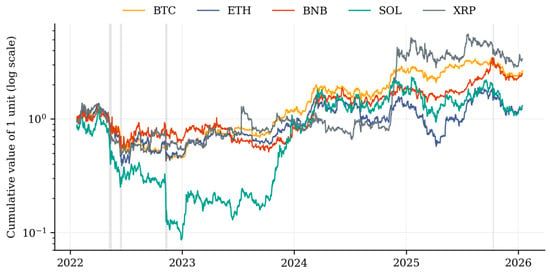
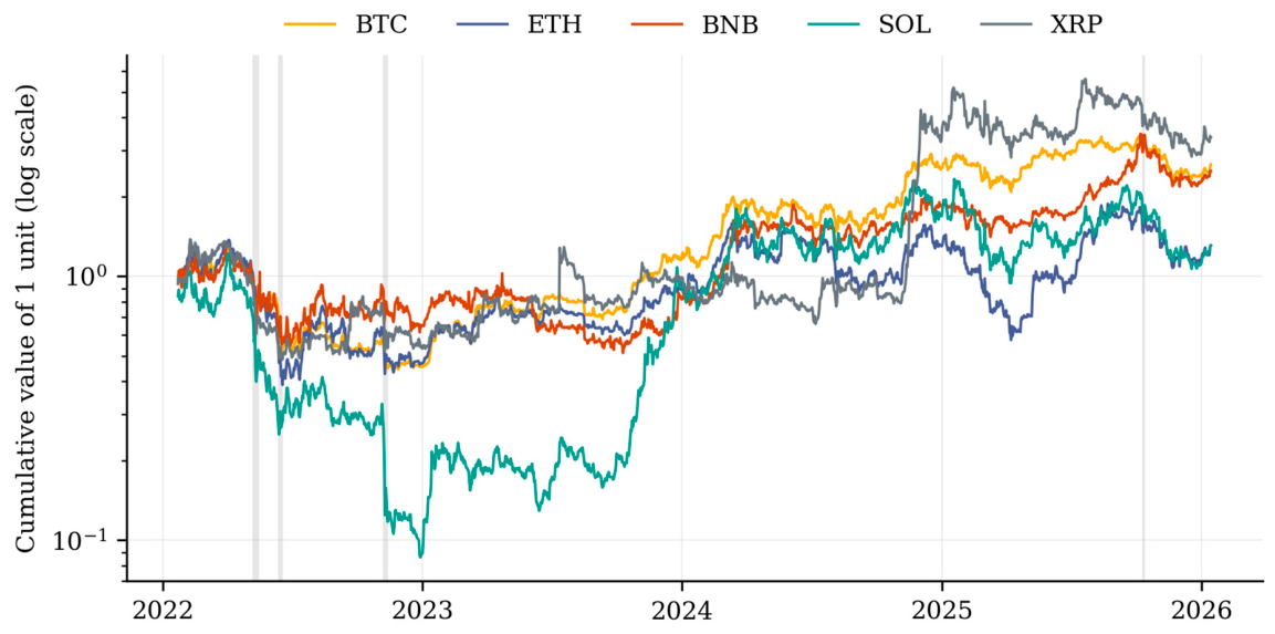
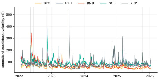
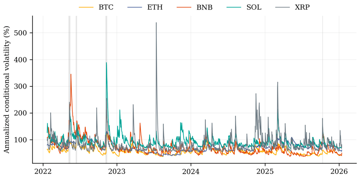
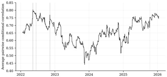
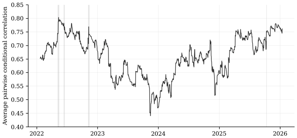
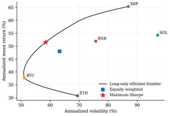
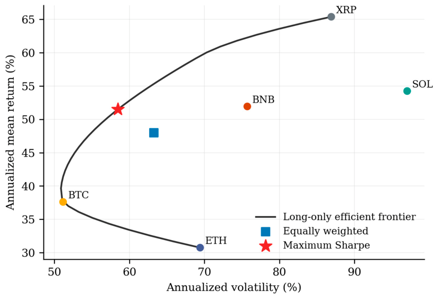
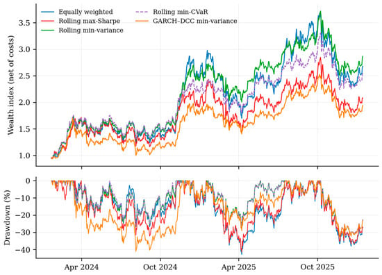
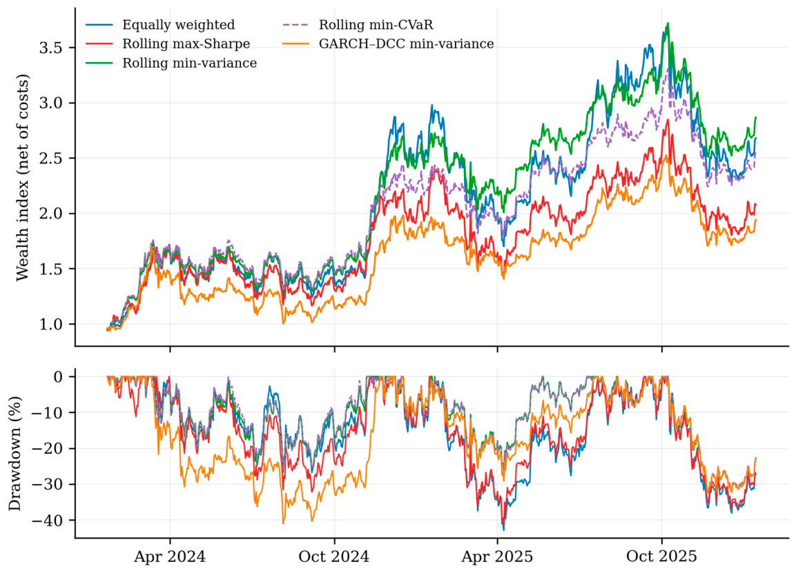
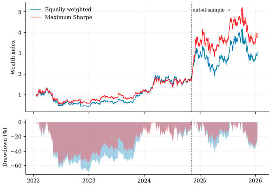
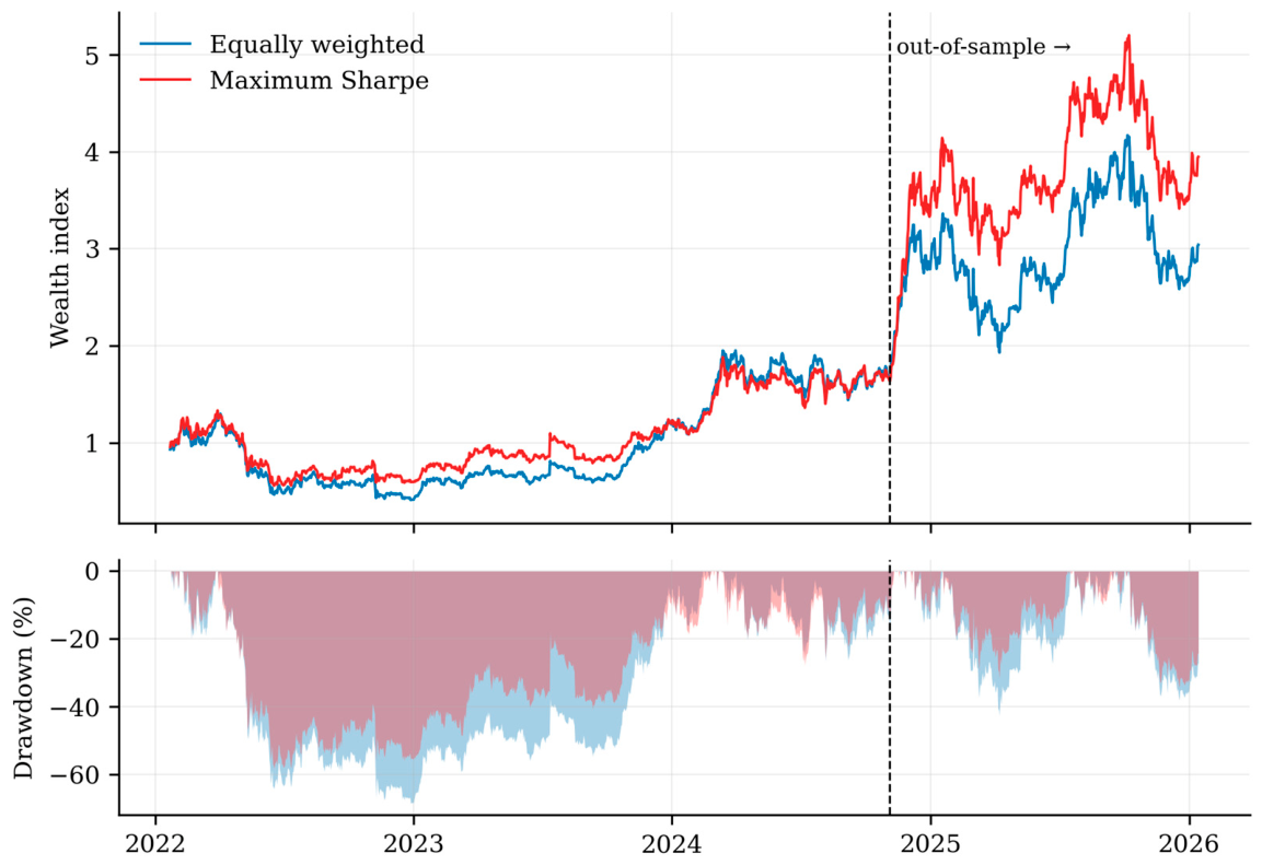
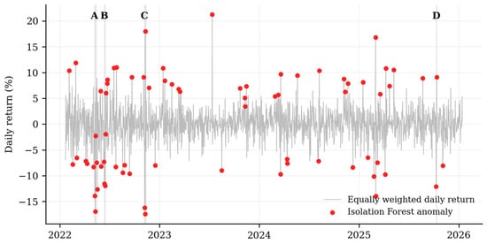
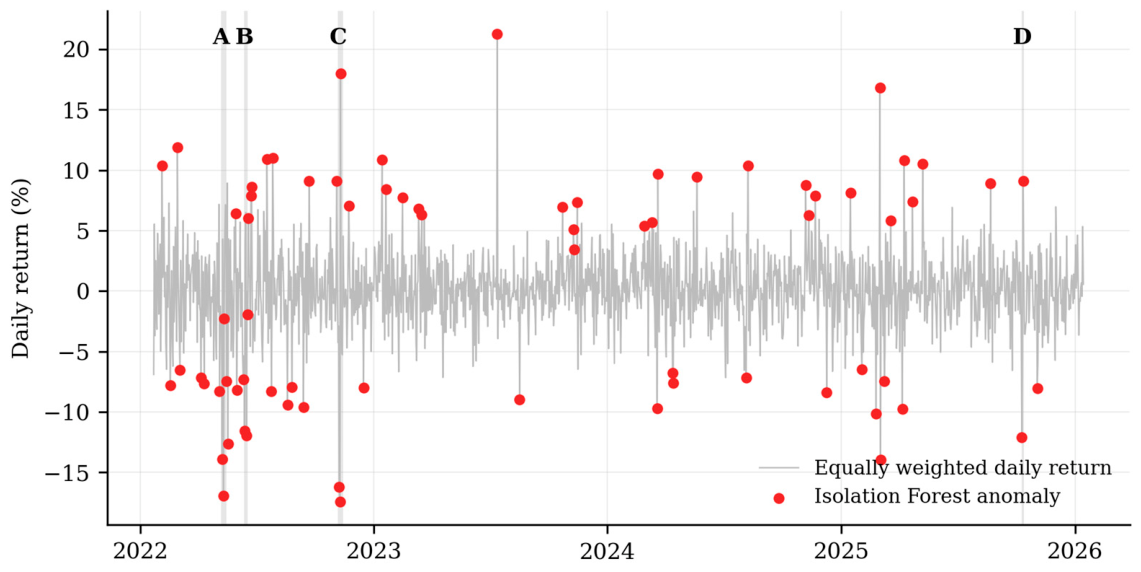

Disclaimer/Publisher’s Note: The statements, opinions and data contained in all publications are solely those of the individual author(s) and contributor(s) and not of MDPI and/or the editor(s). MDPI and/or the editor(s) disclaim responsibility for any injury to people or property resulting from any ideas, methods, instructions or products referred to in the content. |
© 2026 by the authors. Licensee MDPI, Basel, Switzerland. This article is an open access article distributed under the terms and conditions of the Creative Commons Attribution (CC BY) license.