


Abstract
This paper evaluates whether dynamic abnormal performance acts as a transmission channel for macroeconomic policy innovations during crisis regimes. Applying a daily State-Space Fama–French five-factor framework—extended to heteroscedastic specifications across a majority of test assets—dynamic Jensen’s alphas and market betas are recursively estimated via the Kalman filter across 47 international equity markets. Second-stage regressions test policy and orthogonalized exchange rate innovations extracted via OLS detrending. Results confirm broad macroeconomic policy neutrality and market efficiency across 44 markets under extreme stress. However, localized friction-driven departures emerge in specific structural settings, notably the Czech Republic, India, and Mexico.
Keywords:
state-space GARCH (1,1); dynamic equity market performance; time-varying Jensen’s alpha; monetary and fiscal policies JEL Classification:
G11; G12; G13; G14; G15
1. Introduction
Performance evaluation in the management of equity portfolios—comprising large, mid, and small capitalization stocks across both developed and emerging markets—represents a critical concern for investment managers, pension funds, and insurance companies. In a globalized environment, these institutional investors seek to construct efficient portfolios within the risk–return framework through international diversification. This pursuit gains heightened relevance when contrasting equity performance during crisis periods, such as the COVID-19 pandemic—characterized by systemic volatility shocks (Baker et al. 2020; Gormsen and Koijen 2020)—against the relative normalcy of the post-pandemic recovery period.
Since the seminal work of Jensen (1968), a manager’s ability to generate abnormal returns by detecting mispriced financial assets has been the cornerstone of active management. While the single-factor Capital Asset Pricing Model (CAPM) by Sharpe (1964) laid the groundwork in the field, the discipline has evolved toward complex multi-factor frameworks. The Fama and French (2015) five-factor model has emerged as a contemporary standard, allowing for the isolation of abnormal market performance (alpha) after controlling for risks associated with market, size, value, profitability, and investment factors.
Departing from traditional constant parameter estimations, this research implements time-varying State-Space specifications that incorporate heteroscedastic conditional residual variances alongside the Fama and French (2015) model framework. Crucially, to maintain model parsimony and prevent numerical instability, this dynamic framework specifically models the time-varying trajectories of Jensen’s alpha and the systematic market beta, while treating the remaining style factor sensitivities as constant unconditional exposures. This methodology effectively captures the time-varying nature of Jensen’s alpha and systematic risks, overcoming the limitations of fixed-parameter models when faced with high-frequency financial data that typically exhibit leptokurtosis and volatility clustering (Bollerslev 1986; Cont 2001).
The central objective of this study is to establish whether short-run, dynamic abnormal performance in international equity markets acts as an immediate transmission channel for macroeconomic policy interventions during systemic crisis regimes. Understanding this relationship is critical for two primary reasons. First, for institutional investors and risk managers, distinguishing between transient factor risk shifts and genuine asset mispricing is essential for dynamic portfolio allocation during high-volatility events. Second, for monetary and fiscal authorities, evaluating the real-time response of dynamic alpha provides direct empirical feedback on whether emergency liquidity injections and macro policy shocks effectively stabilize pricing mechanisms or inadvertently introduce temporary informational frictions into equity markets.
To ensure optimal goodness-of-fit and parsimony, in most cases, five econometric specifications of the Fama and French (2015) model are contrasted:
- Static OLS: Fixed parameters and constant residual variance.
- OLS-GARCH (1,1): Fixed parameters and conditional residual variance under a GARCH (1,1) process.
- State-Space (Homoscedastic): Dynamic alphas and market betas with fixed sensitivity to the remaining four risk factors and under a constant residual variance.
- State-Space (Heteroscedastic): Dynamic alphas and market betas with fixed sensitivity to the remaining four risk factors and conditional residual variance under a GARCH (1,1) process, Bollerslev (1986).
- State-Space (Heteroscedastic): Dynamic alphas and market betas with fixed sensitivity to the remaining four risk factors and conditional residual variance under a EGARCH (1,1,1) process, Nelson (1991).
Therefore, this study offers three primary contributions to the literature:
First, this study establishes the statistical superiority of advanced State-Space volatility modeling within global equity markets. By utilizing the MSCI World IMI and MSCI Emerging Markets IMI indices—benchmarks widely followed by global institutional investors—the empirical findings confirm that, in most cases, the State-Space GARCH (1,1) and EGARCH (1,1,1) specifications outperform constant parameter alternatives when applied to high-frequency data across developed and emerging markets, respectively. While a standard GARCH (1,1) model assumes a symmetric volatility response to positive and negative innovations—an assumption that frequently fails during market crises—this research leverages the State-Space EGARCH (1,1,1) framework to capture potential asymmetries and the well-documented “leverage effect,” wherein negative shocks generate higher subsequent volatility than positive shocks of equal magnitude. Furthermore, by specifying time-varying alphas and market betas alongside fixed sensitivities for the remaining risk factors, this framework successfully mitigates the Kalman filter convergence issues (Brooks 2019) that typically arise from over-parameterization when attempting to model all risk coefficients dynamically.
Second, it maps the evolution of the Fama and French (2015) risk factors through recent macroeconomic shifts. By tracking these factors across both the COVID-19 pandemic and post-pandemic periods, the study offers a comprehensive comparative analysis of how stock market performance and systematic risk dynamics diverged between developed and emerging market regimes.
Third, and most significantly, it quantifies the asymmetric impacts of economic policies. It identifies how independent monetary and fiscal policies and exchange rate shocks influence equity performance, providing critical empirical evidence on how these macroeconomic innovations can either catalyze or constrain stock market outcomes.
The remainder of this article is organized as follows. Section 2 reviews the relevant literature, while Section 3 presents the Fama and French (2015) model alongside the econometric estimation methods. Section 4 describes the sample and data utilized in the study. Section 5 reports the stock market performance results. Section 6 details the second-stage empirical design, focusing on macroeconomic policy shocks and the relationship with stock market performance, followed by Section 7, which discusses the interaction between stock market performance and macroeconomic policy innovations. Section 8 presents the methodological boundaries and future research lines, and finally, Section 9 concludes the article.
2. Literature Review
The performance evaluation literature has progressively evolved from static, single-factor measures toward dynamic, multi-factor specifications. This section synthesizes relevant theoretical and empirical findings into a focused framework centered on dynamic factor pricing, state-space modeling, and macroeconomic policy transmission during crisis windows.
2.1. Theoretical Foundations and Dynamic State-Space Modeling
The foundational measure of abnormal performance, Jensen’s alpha (Jensen 1968), was established under the static single-factor Capital Asset Pricing Model (Sharpe 1964; Sandoval and Germany 2018). While multi-factor specifications—such as the Fama and French (2015) five-factor model—resolve CAPM’s primary theoretical limitation by controlling for size, value, profitability, and investment risk dimensions, standard fixed-parameter formulations still assume time-invariant risk–pricing relationships.
Consequently, static models remain incapable of capturing short-run efficiency shocks or transient mispricing during severe crisis regimes. To track the temporal dynamics of asset returns, the performance evaluation literature has increasingly adopted state-space architectures. Precedents established by Mamaysky et al. (2008) demonstrate that Kalman filter tracking of latent, mean-reverting mutual fund alphas and betas effectively captures structural risk shifts. Similarly, Adrian and Franzoni (2009) show that unobserved time variation in factor exposures explains pricing anomalies that static models miss entirely. Building upon these architectures, this study jointly tracks unobserved time-varying alpha (αt) and market beta (βmkt,t) parameters within a multi-factor Fama–French framework, integrated with asymmetric conditional heteroscedasticity across a global panel of 47 sovereign equity markets during the COVID-19 pandemic and post-pandemic periods. Constraining secondary style factor loadings (SMB, HML, RMW, CMA) to a fixed baseline stabilizes the filter, isolating daily abnormal performance from broad market volatility.
To account for structural instability and non-linear parameter dynamics during extreme market stress, recent asset pricing literature emphasizes the necessity of modeling time-varying risk exposures and regime shifts. Ang and Timmermann (2011) and Guidolin and Timmermann (2008) demonstrate that conditional returns and factor exposures undergo rapid, discrete transitions across market states, making static linear models insufficient during systemic shocks. In this context, Guidolin (2011) highlights how failing to incorporate structural breaks distorts optimal asset allocation and risk estimation. Econometrically, Abdymomunov and Morley (2011) show that dynamic state-space frameworks effectively capture time variation in both systematic market risk and localized alpha, while Turtle and Zhang (2015) confirm that modeling conditional volatility shifts alongside time-varying parameters significantly improves empirical factor model performance across distinct market regimes.
2.2. Dynamic Pricing and Heteroscedasticity Across International Markets
Empirical factor sensitivities vary significantly by the degree of market development and experience severe disruptions during systemic crisis events (Tarakcioglu et al. 2023; Sandoval and Molina 2022). In emerging and frontier market contexts, local idiosyncratic risks, market segmentation, and liquidity shocks frequently dominate globally integrated factors (Mosoeu and Kodongo 2022; Mbengue et al. 2023). Standard fixed-coefficient linear regressions fail to capture these non-linear dynamics and persistent variance clustering during acute market panics (Goo and Wang 2024; Huber et al. 2023).
Integrating dynamic state-space parameter tracking with conditional error volatility specifications (GARCH and EGARCH) is therefore essential to isolate genuine excess return dynamics from estimation bias and crisis-induced variance spikes (Liu et al. 2025; Laopodis 2025). This combined framework adheres to three core modeling principles: (1) multi-factor baseline controls to mitigate omitted variable bias; (2) dynamic state tracking of latent alpha and market beta trajectories; and (3) heteroscedastic error equations to accommodate volatility clustering.
2.3. Macroeconomic Policy Channels and Dynamic Performance
A distinguishing component of this study is the evaluation of how latent alpha trajectories interact with real-world macroeconomic policy innovations during crisis windows. From a theoretical perspective, expansionary monetary policy reduces the cost of capital by lowering real interest rates (Mishkin 1996) while strengthening balance sheet collateral values and reducing external financing premiums (Bernanke and Gertler 1995). Concurrently, expansionary fiscal policy acts as a direct catalyst for aggregate demand, enabling sector-specific cash flow recoveries (Blanchard and Perotti 2002).
By evaluating state-space risk parameters alongside macroeconomic policy indicators across diverse international equity markets, this article fills a critical literature gap—reconciling dynamic factor pricing and short-term market efficiency with empirical macro policy variations across sovereign markets.
3. Model and Econometric Methods of Estimation
The Fama and French (2015) five-factor model is a multivariate linear framework that takes, in its empirical form, the following expression:
where
Rjt − Rft = βj1t(Rmt − Rft) + βj2SMBt + βj3HMLt + βj4RMWt + βj5CMAt + ujt
- Rjt is the realized return on portfolio j in period t.
- Rft is the risk-free rate in period t.
- (Rmt − Rft) is the realized market risk premium in period t.
- (SMBt) is the realized return differential between small-cap and large-cap portfolios in period t (Small Minus Big).
- (HMLt) is the realized return differential between high- and low-book-to-market equity portfolios in period t (High Minus Low).
- (RMWt) is the realized return differential between portfolios of robust and weak profitability firms in period t (Robust Minus Weak).
- (CMAt) is the realized return differential between portfolios of conservative and aggressive investment firms in period t (Conservative Minus Aggressive).
Furthermore, the coefficients βj1t, βj2, βj3, βj4, βj5 are assumed to capture the dynamic sensitivity of portfolio j to the market factor and the unconditional sensitivities to the remaining four risk factors, respectively.
The Fama–French five-factor model is expressed through Equation (1) in realized data rather than ex-ante expectations. Deriving this equation assumes that stock markets are efficient in a fair game sense. However, if this efficiency fails to hold over time, it may lead to abnormal performance relative to the equilibrium return-generating process. To account for this, we incorporate a dynamic alpha, αjt y αkt (Jensen’s alpha) for both the COVID-19 pandemic period (d1 = 1 during the pandemic, 0 otherwise) and the post-pandemic period (d2 = 1 during the post-pandemic period, 0 otherwise). Thus, Equation (1) is rewritten as:
A critical econometric consideration in estimating multi-factor asset pricing models via state-space representation concerns the balance between parameter flexibility and computational stability. In Equation (2), time variation is explicitly restricted to the intercept alpha and the primary market exposure beta, while style factor loadings (SMB, HML, RMW, CMA) remain fixed across sub-periods. This specification is methodologically grounded in three key principles:
First, from a parsimony and estimation stability standpoint, allowing all factor loadings to vary simultaneously in a dynamic state-space filter significantly inflates the dimension of the state vector. In continuous daily estimation across international panels, high-dimensional state-space models frequently suffer from over-parameterization, non-positive definiteness of the variance–covariance matrix, and optimization instability in Kalman filter convergence. Constraining secondary style loadings fixes the baseline coordinates of the risk space, enabling the filter to reliably isolate dynamic adjustments in excess returns alpha and systematic market sensitivity beta without absorbing estimation noise.
Second, market risk beta represents the primary transmission channel for macro-financial shocks and systemic liquidity drawdowns during crisis episodes, whereas firm-level style attributes (e.g., market capitalization, book-to-market ratios, profitability, and investment) evolve at structural, lower-frequency horizons. Fixing style loadings ensures that sub-period dummy indicators d1 and d2 cleanly split baseline shifts in mean risk-adjusted performance without distorting the structural baseline risk exposures across distinct economic regimes (Fama and French 2020).
Finally, this hybrid formulation aligns with the established regime-switching and time-varying parameter literature (e.g., Bianchi et al. 2015), which demonstrates that maintaining constant loadings on secondary factors provides a controlled benchmark for detecting genuine parameter drift in systematic risk and unmodeled abnormal performance during acute market disruptions.
Statistically, the coefficient αjt in Equation (2) may be positive, negative, or zero on any given day. A statistically significant positive value captures superior performance, while a negative value indicates inferior performance relative to the returns generated by the dynamic Fama and French (2015) fair game model. A value of zero indicates normal performance. In line with state-space modeling nomenclature, Equation (2) therefore represents the observation equation, while the following equations represent the transition (state) equations:
The dynamics of the time-varying coefficients of Equations (3)–(5) are assumed to follow a mean-reverting process, following specifications suggested by Brooks et al. (2000), Groenewold and Fraser (1999), and Ortas et al. (2015).
Under the Adaptive Market Hypothesis, a statistically significant state-space alpha in Equation (2) signals a persistent departure from factor-implied efficiency. Tracking this alpha after a policy shock shows how quickly the market returns to equilibrium. Moreover, a rapid mean reversion of alpha to zero indicates efficient information processing, while persistent non-zero trajectories highlight structural frictions.
To explicitly capture the severe excess kurtosis and heavy tails inherent in daily sovereign equity returns, the unknown parameters of the system (Equations (3)–(5)) are estimated by maximizing a Student-t log-likelihood function (Harvey 1990) rather than a standard Gaussian function:
where ) is the expanded vector of hyperparameters, including the degrees of freedom parameters (v), Γ(∙) represents the Gamma function, et, represents the prediction errors, and their conditional variance is recursively estimated using the Kalman filter. Initial values for the hyperparameters are set according to Wells (1996); specifically, an initial value of 0.1 is used for the coefficients capturing the speed at which the time-varying alphas and betas revert to their mean. An initial variance of e−1 is set for the residuals of Equations (3)–(5).
On the other hand, in the financial econometric literature, it is widely recognized that daily returns of risky assets exhibit volatility clustering, which becomes more pronounced during crises. These phenomena can be, in most cases, well captured by either a GARCH (1,1) model or an EGARCH (1,1,1) model. Consequently, it is more realistic to assume that the residuals of the observation Equation (2) follow a conditionally heteroscedastic process:
where
under a GARCH(1,1) model.
It is important to note that the standard GARCH (1,1) model assumes a symmetric response of volatility to positive and negative shocks, an assumption that frequently fails during periods of crisis. To address potential asymmetries and capture the well-documented “leverage effect”—where negative shocks generate higher subsequent volatility than positive shocks of equal magnitude—the GARCH (1,1) model is contrasted with a State-Space EGARCH(1,1,1) model. The conditional variance under the EGARCH framework is modeled in logarithmic form according to Equation (9) as follows:
In Equation (9), the parameter gamma captures the asymmetric leverage effect. If gamma < 0, it implies that bad news (negative innovations) increases conditional volatility more than good news (positive innovations), a characteristic highly relevant for analyzing market behavior during major external shocks such as the COVID-19 pandemic. Furthermore, modeling relaxes the strict non-negativity constraints on the coefficients: omega , chi , gamma and beta, βj,1, providing greater numerical stability during estimation.
The parameters are estimated via a two-step iterative procedure. First, the hyperparameters of the state-space system are estimated under a homoscedastic assumption to generate the initial prediction residuals. Second, the resulting residuals are utilized to model the conditional variance dynamics via either Equation (8) or Equation (9), selecting the optimal specification according to the information criteria.
To ensure that the final state-space specifications captured the conditional variance dynamics and eliminated any remaining heteroscedasticity, a post-estimation diagnostic framework was implemented for the GARCH (1,1) and EGARCH (1,1,1) residuals based on the best-fitting model according to the information criteria for each stock market under study. First, the Ljung–Box test was applied to both the standardized residuals and squared standardized residuals using 20 lags. This choice follows standard practices for daily data (Diebold 2007; Tsay 2010), ensuring that persistent volatility dependencies are captured (see results in Appendix B and Appendix C for developed and emerging stock markets, respectively). Second, the autoregressive conditional heteroskedasticity Lagrange Multiplier (ARCH-LM) test was executed, validating that the residuals behaved as homoscedastic white noise with no remaining ARCH effects (see results in Appendix B and Appendix C for developed and emerging stock markets, respectively).
Finally, the selected conditional variance process was integrated back into the observation Equation (2), and the entire state-space system was re-estimated simultaneously to produce the final time-varying parameters. Crucially, during this final simultaneous estimation, the baseline Gaussian innovation assumption was evaluated and replaced with a Student-t distribution framework. Given the severe excess kurtosis and fatter-than-normal tails observed across the dataset, the Student-t distribution was retained for all 47 markets under study to guarantee that the final estimations accommodate leptokurtic innovations. The resulting estimated degrees of freedom (v) for each market’s dominant heteroscedastic model are reported alongside model selection criteria in Appendix D and Appendix E.
4. Sample and Data
Data for the equity indices of 23 developed markets and 24 emerging markets—classified according to the MSCI ACWI IMI (Investable Market Index)—were retrieved from the MSCI website (www.msci.com), accessed on 1 February 2026. These indices are fundamental for calculating daily returns in U.S. dollars. The sample period spans from 10 March 2020 to 5 May 2023, yielding 823 daily returns (calculated from 11 March 2020 to 5 May 2023). This timeframe covers the onset through the official conclusion of the COVID-19 pandemic, in accordance with World Health Organization (WHO) announcements. Subsequently, a post-pandemic period is considered, with daily returns ranging from 8 May 2023 to 31 October 2025—the latest date for which Fama–French global risk factors were available for both developed and emerging markets—resulting in 650 daily returns per market.
The MSCI IMI for each country captures the performance of a representative portfolio covering 99% of the free-float-adjusted market capitalization across large-, mid-, and small-cap segments. The 23 developed markets, 24 emerging markets, and the MSCI World and Emerging Markets IMI indices (used as respective benchmarks) are listed in Table 1, Table 2, Table 3 and Table 4, later in this article. MSCI classifies these markets based on three general criteria: economic development, size and liquidity requirements, and market accessibility. Further specific criteria used for filtering and classification are available on the MSCI website. The daily yield of one-month U.S. Treasury bills is used as the risk-free rate. The remaining Fama–French risk factors, along with the risk-free rate, were extracted at a daily frequency from Kenneth French’s data library.
Table 1.
Descriptive statistics of excess returns for MSCI IMI developed market equity indices: 11 March 2020 to 5 May 2023 (COVID-19 pandemic start–end period).
Table 2.
Descriptive statistics of excess returns for MSCI IMI developed market equity indices, from 8 May 2023 to 31 October 2025. Post-COVID-19 pandemic period.
Table 3.
Descriptive statistics of excess returns for MSCI IMI Emerging Markets equity indices, from 11 March 2020 to 5 May 2023. COVID-19 pandemic start–end period.
Table 4.
Descriptive statistics of excess returns for MSCI IMI emerging market equity indices, from 8 May 2023, to 31 October 2025. Post-COVID-19 pandemic period.
https://mba.tuck.dartmouth.edu/pages/faculty/ken.french/data_library.html, accessed on 1 February 2026.
To accurately capture the high-frequency transmission mechanism between macroeconomic policy shocks and factor-adjusted abnormal performance, all estimations were conducted using daily frequency data. Emergency policy announcements, central bank interventions, and fiscal relief packages demand a fast portfolio reallocation. Estimating the state-space model at lower frequencies (e.g., monthly or quarterly) introduces severe time aggregation bias, effectively smoothing out acute volatility clusters and short-lived dynamic alpha trajectories. A daily frequency is therefore essential to isolate the exact empirical window during which macro policy innovations impact equity market efficiency.
Table 1 presents the descriptive statistics for the daily excess returns of the 23 developed market equity indices, alongside the MSCI World IMI index used as the benchmark. The statistics cover the COVID-19 pandemic period. The JB column reports the test statistics for the Jarque–Bera normality test. The ADF column displays the results of the Augmented Dickey–Fuller unit root test, with lag lengths selected based on the Schwarz Information Criterion (SIC). The LB2 column reports the Ljung–Box test statistics for the squared daily excess returns of each equity market. In accordance with Tsay (2005), the number of lags for this test was determined by the natural logarithm of the number of observations, ln (823) ≈ 7. Source: Own elaboration based on EViews 13.0 outputs.
Table 1 presents the descriptive statistics for the daily excess returns of the 23 MSCI IMI equity indices within the developed markets group during the pandemic period (11 March 2020 to 5 May 2023). The highest average daily excess return was recorded by the Denmark index (0.0813%), followed by the Netherlands (0.0610%). Conversely, the lowest average daily excess returns were observed in Hong Kong (−0.0021%) and Singapore (−0.0003%), respectively. Regarding risk—measured by the standard deviation of daily excess returns—the Switzerland index exhibited the lowest volatility, while the highest risk was captured by the Austria index. All daily excess return series for the indices reported in Table 1 display negative skewness, with the exceptions of Japan, Hong Kong, and Singapore; that is, the majority (20 out of 23) present a distribution skewed toward negative excess returns. Furthermore, the series exhibit high levels of leptokurtosis, indicating distributions that are more peaked and have fatter tails compared with a normal distribution. The Jarque–Bera test results confirm the rejection of the null hypothesis of normality for all series under study. Additionally, the Augmented Dickey–Fuller (ADF) test confirms the rejection of the null hypothesis of a unit root, establishing that all excess return series are stationary. Finally, the Ljung–Box test indicates that all series are heteroscedastic; this suggests that controlling for the residuals of Equation (4) through their conditional variance (Equation (9)), as proposed in this article, is more appropriate than assuming traditional homoscedastic behavior.
Table 2 presents the descriptive statistics for the daily excess returns of the 23 stock indices and the MSCI World IMI index as a benchmark, covering the post-COVID-19 pandemic period. The JB column reports the values for the Jarque–Bera normality test. The ADF column displays the results of the Augmented Dickey–Fuller unit root test, where the lag lengths were determined based on the Schwarz Information Criterion (SIC). The LB2 column provides the Ljung–Box test statistics for the squared daily excess returns of each equity market. Following Tsay (2005), the number of lags for this test was set according to the natural logarithm of the number of observations, ln (650) ≈ 7. Source: Own elaboration based on EViews 13.0 outputs.
Table 2 presents the descriptive statistics for the daily excess returns of the 23 equity indices within the developed markets set during the post-pandemic period (8 May 2023 to 31 October 2025). The highest average daily excess return was achieved by the Israeli index (0.0875%), followed by Spain (0.0845%). Conversely, the lowest average daily excess returns were recorded by Denmark (−0.0354%) and New Zealand (−0.0307%), respectively.
Regarding risk, as measured by the standard deviation of daily excess returns, the Singaporean index exhibited the lowest volatility, while the Danish index captured the highest risk. Sixteen out of the twenty-three daily excess return series reported in Table 2 display negative skewness, while seven series—Austria, Finland, Germany, Sweden, Australia, New Zealand, and the USA—show positive skewness. This indicates that the majority of the distributions are skewed toward negative excess returns. Furthermore, the series exhibit high levels of leptokurtosis, characterized by more peaked distributions and fatter tails compared to a normal distribution. The results of the Jarque–Bera test confirm the rejection of the null hypothesis of normality for all series under study. Similarly, the Augmented Dickey–Fuller (ADF) test confirms the rejection of the unit root null hypothesis, establishing that all excess return series are stationary. Finally, the Ljung–Box test indicates that all series are heteroscedastic, with the exception of Denmark, the Netherlands, and Israel. This suggests that the control proposed in this study for the residuals of Equation (4) via conditional variance, Equation (9), is more appropriate than a traditional homoscedastic approach.
Comparing both periods reveals that the performance of the MSCI World IMI index was lower during the pandemic than in the post-pandemic period. The pandemic period was characterized by a lower average return (0.0426% versus 0.0495%) and higher risk (1.2870% versus 0.7878%), resulting in Sharpe ratios of 0.0331 and 0.0628 for the pandemic and post-pandemic periods, respectively. This provides preliminary descriptive evidence of the negative impact of the pandemic on the performance of developed equity markets.
Table 3 presents the descriptive statistics for the daily excess returns of the 24 emerging market equity indices, alongside the MSCI Emerging Markets IMI index used as a benchmark. The statistics cover the COVID-19 pandemic period. The JB column reports the values associated with the Jarque–Bera normality test, while the ADF column displays the results of the Augmented Dickey–Fuller unit root test. Lags for the ADF test were determined based on the Schwarz Information Criterion (SIC). The LB2 column reports the Ljung–Box test statistics for the squared daily excess returns of each equity market. Following the suggestion of Tsay (2005), the number of lags for this test was determined by the natural logarithm of the number of observations, ln (823) ≈ 7. Source: Own elaboration based on EViews 13.0 outputs.
Table 3 presents the descriptive statistics for the daily excess returns of the 24 MSCI EM IMI equity indices within the emerging markets group during the pandemic period (11 March to 5 May 2023). The highest mean daily excess return was recorded by the Czech Republic index (0.0938%), followed by Greece (0.0785%). Conversely, the lowest mean daily excess returns were observed for Egypt (−0.0302%) and Colombia (−0.0180%), respectively. Regarding risk, as measured by the standard deviation of daily excess returns, the Kuwaiti index exhibited the lowest volatility, whereas the highest risk was captured by the Turkish index. The majority of the daily excess return series reported in Table 3 exhibit negative skewness. The exceptions are China, Indonesia, Korea, Malaysia, Taiwan, and Turkey; thus, most distributions are skewed toward negative excess returns. Furthermore, the series display high levels of leptokurtosis, characterized by more peaked distributions and fatter tails compared to a normal distribution. Examining the Jarque–Bera test results confirms the rejection of the null hypothesis of normality for all series under study. Additionally, the Augmented Dickey–Fuller (ADF) test results reject the null hypothesis of a unit root, indicating that all excess return series are stationary. Finally, the Ljung–Box test demonstrates that all series exhibit heteroscedasticity. This indicates that controlling for the residuals of Equation (4) through their conditional variance—as proposed in Equation (9)—is more appropriate than assuming traditional homoscedastic behavior.
Table 4 presents the descriptive statistics for the daily excess returns of 24 emerging market equity indices, including the MSCI Emerging Markets IMI as a benchmark, for the post-COVID-19 pandemic period. The JB column reports the values for the Jarque–Bera normality test. The ADF column displays the results of the Augmented Dickey–Fuller unit root test, with lag lengths determined by the Schwarz Information Criterion (SIC). The LB2 column displays the Ljung–Box test statistics for the squared daily excess returns of each equity market. Following Tsay (2005), the number of lags for this test was determined based on the natural logarithm of the number of observations, ln (650) ≈ 7. Source: Own elaboration based on EViews 13.0 outputs.
Table 4 presents the descriptive statistics for the daily excess returns of the 24 stock indices within the emerging markets set during the post-pandemic period (8 May 2023 to 31 October 2025). The highest average daily excess return was achieved by the Hungarian index (0.1076%), followed by Colombia (0.1041%). Conversely, the lowest average daily excess returns were recorded by Indonesia (−0.0511%) and Thailand (−0.0355%), respectively.
Regarding risk, as measured by the standard deviation of daily excess returns, the Kuwaiti index exhibited the lowest risk, while the Egyptian index captured the highest. Nineteen out of the twenty-four daily excess return series associated with the indices reported in Table 4 display negative skewness, whereas five series—Hungary, Peru, Poland, South Africa and Thailand—show positive skewness. This indicates that the majority of the distributions are skewed toward negative excess returns. Furthermore, the series exhibit high levels of leptokurtosis, characterized by more peaked distributions and fatter tails compared to a normal distribution. The Jarque–Bera test results confirm the rejection of the null hypothesis of normality for all series under study. Additionally, the Augmented Dickey–Fuller (ADF) test rejects the null hypothesis of a unit root, confirming that all excess return series are stationary. Finally, the Ljung–Box test shows that nearly all series are heteroscedastic, with the exceptions of Brazil and Egypt. This suggests that the control proposed in this study for the residuals of Equation (4) through its conditional variance, Equation (9), is more appropriate than a traditional homoscedastic approach.
A comparison of both periods reveals that the performance of the MSCI EM IMI stock index was lower during the pandemic than in the post-pandemic period. The pandemic period exhibited a lower average return (0.0090% vs. 0.0386%) and higher risk (1.1727% vs. 0.8539%), resulting in Sharpe ratios of 0.0077 and 0.0452 for the pandemic and post-pandemic periods, respectively. This provides preliminary descriptive evidence of the negative impact of the pandemic on the performance of emerging equity markets.
In global terms, the descriptive statistics reported in Table 1, Table 2, Table 3 and Table 4—encompassing average excess returns and total risk for both developed and emerging equity markets—confirm better stock market performance, as measured by the Sharpe ratio, for the developed markets set (MSCI World IMI) compared with emerging markets (MSCI EM IMI), both during and after the COVID-19 pandemic.
5. Stock Market Performance Results
Table 5 and Table 6 report the coefficients capturing superior (+), normal (0), or inferior (−) stock market performance, represented by the alpha coefficients for the pandemic period and for the post-pandemic period, across developed and emerging equity markets. The reported coefficients focus on mean-reverting values to demonstrate whether a process converges toward persistent and statistically significant long-term values within each evaluated period. Only the results from the best-fitting specification among the five previously mentioned are reported, based on the frequency with which the information criteria favor a specific model. Thus, if a particular specification outperforms the others in two or three of the criteria, it is reported as the best model.
Table 5.
Pre-and post-COVID-19 Alphas and sensitivity coefficients of developed equity market returns relative to the Fama and French (2015) five-factor model. From 11 March 2020 to 5 May 2023 (Pre-COVID-19). From 8 May 2023 to 31 October 2025 (Post-COVID-19).
Table 6.
Pre- and post-COVID-19 pandemic alphas and sensitivity coefficients of emerging stock market returns relative to the Fama and French (2015) five-factor model. From 11 March 2020 to 5 May 2023 (Pre-COVID-19). From 8 May 2023 to 31 October 2025 (Post-COVID-19).
Upon contrasting the five specifications, the results for the developed stock markets—based on the AIC, BIC, and HQ information criteria—confirm that Specification 4 (State-Space GARCH(1,1)) dominates in 14 out of 23 cases, Specification 5 (State-Space EGARCH(1,1,1)) dominates in 3 out of 23 cases, Specification 3 (homoscedastic State-Space) dominates in 4 out of 23 cases, and Specification 2 dominates in just 1 out of 23 cases, specifically the Hong Kong stock market (see Appendix D for the information criteria values of the five specifications). In addition, none of the developed stock markets show any remaining GARCH effects after estimating Specifications 4 and 5, with the exception of Australia, where the remaining heteroscedasticity was eliminated after estimating a GARCH(3,3) process; its information criteria (see Appendix D for the information criteria values of the five specifications).
The results for the emerging stock markets, based on the AIC, BIC, and HQ information criteria, confirm that Specification 4 (State-Space GARCH(1,1)) dominates in 4 out of 24 cases, Specification 5 (State-Space EGARCH(1,1,1)) dominates in 11 out of 24 cases, and Specification 2 dominates in 6 out of 24 cases. In addition, none of the emerging stock markets show any remaining GARCH effects after estimating Specifications 2, 4, and 5, with the exception of Indonesia, Qatar, and Saudi Arabia. For these markets, the remaining heteroscedasticity was eliminated after estimating an EGARCH(2,1,1), a GARCH(5,0), and an EGARCH(5,5,1) process, respectively; their information criteria (see Appendix E for the information criteria values of the five specifications).
Table 5 presents the alphas during the pandemic period in the third column, while the fourth column reports the post-pandemic alphas. Regarding the sensitivity coefficients for the five risk factors—market, size, value, profitability, and investment—these are displayed in the fifth, sixth, seventh, eighth, and ninth columns, respectively. Source: Own elaboration based on EViews 13.0 outputs.
The results reported in Table 5 indicate that none of the developed equity markets under study exhibit statistically significant (at the 1% or 5% levels) mean-reverting alphas during and after the pandemic period. Regarding systematic market risk (Rm-Rf), all twenty-three equity markets display mean-reverting betas that are statistically significant at the 1% level. Sweden is the riskiest market with a beta of 1.2147, while Hong Kong is the least risky with a beta of 0.4777.
In relation to the size risk factor (SMB), four out of the twenty-three markets—the Netherlands, Sweden, Hong Kong, and Singapore—do not show statistically significant sensitivity in their respective stock returns. Regarding the value risk factor (HML), two markets (Belgium and Singapore) lack statistically significant sensitivity. Conversely, for the profitability risk factor (RMW), all twenty-three equity markets exhibit return sensitivity that is statistically significant at the 1% level. Finally, concerning the investment risk factor (CMA), eighteen out of twenty-three markets do not show statistically significant sensitivity; these include Austria, Belgium, Denmark, Finland, France, Germany, Ireland, Italy, Portugal, Spain, the United Kingdom, Australia, Hong Kong, Japan, New Zealand, Singapore, the United States, and Israel.
In summary, among the five risk factors, those demonstrating the highest statistical significance regarding the sensitivity of developed equity market returns are systematic market risk (Rm—Rf) and profitability (RMW), both across 100% of tested markets. These are followed by the value factor (HML) at 91%, size (SMB) at 83%, and finally, the investment factor (CMA) at only 22%. The results reveal that none of the twenty-three developed equity markets exhibit statistically significant mean-reverting alphas during or after the pandemic. From an asset pricing perspective, this implies that alphas are statistically indistinguishable from zero, confirming that the Fama–French five-factor model maintains strong explanatory power even under extreme market stress. Rather than generating structural mispricing, the pandemic-induced volatility was absorbed entirely by the time-varying sensitivity of systematic risk factors—most notably the market risk (Rm—Rf) and profitability (RMW) channels—validating the semi-strong form of market efficiency across the developed stock markets under study.
Table 6 presents the alphas during the pandemic period in the third column, while the fourth column reports the post-pandemic alphas. Regarding the sensitivity coefficients for the five risk factors—market, size, value, profitability, and investment—these are displayed in the fifth, sixth, seventh, eighth, and ninth columns, respectively. Source: Own elaboration based on EViews 13.0 outputs.
The results reported in Table 6 demonstrate that four of the emerging equity markets under study exhibit positive, statistically significant mean-reverting alphas during the pandemic period. The most notable cases include the Czech Republic with +0.1165% per day (+29.36% annualized, significant at the 5% level), Mexico with +0.0777% per day (+19.58% annualized, at the 5% level), India with +0.0771% per day (+19.43% annualized, at the 5% level), and Saudi Arabia with +0.0452% per day (+11.39% annualized, at the 5% level). The sole negative case corresponds to China, the country where the pandemic originated, with −0.0526% per day (−13.26% annualized, at the 5% level). In the post-pandemic period, one equity market shows a negative statistically significant alpha: Thailand, with an alpha of −0.0877% per day (−22.10% annualized, significant at the 5% level).
Regarding systematic market risk (Rm-Rf), all twenty-four equity markets display statistically significant mean-reverting betas at the 1% level. China emerges with the highest systematic beta risk of 1.4122, while Kuwait shows the lowest with a beta risk of 0.2204. In relation to the size risk factor (SMB), eleven of the twenty-four markets—Egypt, India, Indonesia, Korea, Kuwait, the Philippines, Qatar, Saudi Arabia, Taiwan, Thailand, and the UA Emirates—show no statistically significant sensitivity in their respective equity returns. Concerning the value risk factor (HML), fifteen markets do not exhibit statistically significant sensitivity: the Czech Republic, Egypt, Greece, Hungary, India, Indonesia, Kuwait, the Philippines, Poland, Qatar, Saudi Arabia, South Africa, Thailand, Turkey, and the UA Emirates.
For the profitability risk factor (RMW), fourteen markets—Chile, the Czech Republic, Egypt, Greece, Hungary, India, Indonesia, the Philippines, Poland, Saudi Arabia, South Africa, Thailand, Turkey, and the UA Emirates—lack statistically significant sensitivity. Finally, regarding the investment risk factor (CMA), eleven markets show no statistically significant sensitivity: the Czech Republic, Egypt, India, Indonesia, Korea, Kuwait, Qatar, Saudi Arabia, Taiwan, Thailand, and the UA Emirates.
In summary, among the five risk factors, those demonstrating the highest statistical significance regarding the sensitivity of emerging market returns are: systematic market risk (Rm-Rf) at 100%, followed by the size factor (SMB) at 54%, investment (CMA) at 54%, profitability (RMW) at 42%, and finally value (HML) at only 38%.
To enhance the interpretability of the econometric framework, Figure 1 illustrates the daily trajectories of the filtered time-varying Jensen’s alphas obtained via the optimal heteroscedastic state-space specifications, explicitly bounded by their corresponding 2RMSE (Root Mean Squared Error) bands used to represent the statistical 95% confidence intervals. Figure 1A,B display the paths for representative developed stock markets (France and Spain), where the conditional variance errors explicitly account for leptokurtosis through Student-t innovations. Because both markets optimize under dynamic, time-varying state configurations across both analyzed temporal horizons, they provide a continuous visual baseline of mature stock market behavior. Their trajectories are characterized by highly stable, tightly bounded mean-reverting horizons clustered near the zero axis—with their 2RMSE tracking bands compressed inside a narrow range of approximately 0.05% to 0.15% daily—visually reinforcing how deep, informationally efficient markets rapidly process and fully discount short-term macro policy surprises over time.
Figure 1.
Time-Varying Jensen’s Alpha Paths with 2RMSE Bands. (Panel (A)) This displays the daily filtered trajectories for the developed stock market of France, exhibiting narrow tracking intervals. (Panel (B)) This displays the daily filtered trajectories for the developed stock market of Spain, exhibiting narrow tracking intervals. (Panel (C)) This displays the paths for the emerging stock market of India, highlighting its expanded risk premia bands. The underlying conditional variance structures explicitly account for leptokurtosis through Student-t innovations. (Panel (D)) This displays the paths for the emerging stock market of Mexico, highlighting its statistically significant positive drift. The underlying conditional variance structures explicitly account for leptokurtosis through Student-t innovations.
Conversely, Figure 1C,D map the trajectories for the emerging market cohort, contrasting India with Mexico. While the Indian alpha path displays severe structural volatility and considerably wider tracking intervals reflecting heightened risk premia under pandemic stress—with its 2RMSE bands expanding significantly to a volatile range of 0.30% to 0.50% daily—it ultimately exhibits a neutral, non-trending horizon centered around zero. In sharp contrast, the alpha path for Mexico (Figure 1D) documents a persistent, structurally distinct upward shift during the pandemic phase. Crucially, this positive drift is statistically meaningful, as the daily alpha trajectory breaks away from zero, climbing toward a positive range of 0.10% to 0.25% daily, with its lower 2RMSE boundary remaining entirely above the zero baseline during the peak of the crisis. This visual divergence cleanly mirrors our subsequent second-stage regression findings, providing clear graphical confirmation that while the vast majority of global markets adhered to strict performance neutrality, Mexico stood out as a uniquely responsive structural anomaly.
To track the evolution of risk dynamics across the sample horizons using an interpretable return scale, Figure 2 plots the daily conditional standard deviation path derived from the best-fittiing heteroscedastic state-space GARCH model for Mexico. The visual evidence reveals a sharp and significant volatility increase coinciding precisely with the first quarter of 2020, capturing the initial onset of the COVID-19 pandemic shock. This extreme risk clustering underscores the structural necessity of our chosen GARCH framework; modeling the state equations under homoscedastic assumptions would have severely understated the standard errors during the peak of the crisis. Notably, Mexico’s daily conditional standard deviation spikes dramatically from its initial pandemic entry levels to an unprecedented crisis peak of 3.5% daily. This extreme surge reflects heightened country risk premiums and severe localized market stress before gradually decaying back toward a more stable, mean-reverting baseline range of 1.0% to 1.5% during the post-pandemic horizon.
Figure 2.
Daily conditional standard deviation path derived from the best-fitting heteroscedastic state-space GARCH model for the Mexico stock market.
The following section explores the potential relationship between dynamic alpha and the monetary and fiscal policies implemented by central banks and government authorities, as well as foreign exchange variations, during both the pandemic and post-pandemic periods.
6. Second-Stage Empirical Design: Macroeconomic Policy Shocks, Currency Movements, and Stock Market Performance
To identify the independent causal effects of monetary policy, fiscal policy, and exchange rate fluctuations on stock market performance, a second-stage time series econometric analysis was introduced. This stage is based on unanticipated macroeconomic shocks and currency innovations. This analysis is exclusively applied to emerging equity markets that exhibited statistically significant mean-reverting alphas during either the pandemic or post-pandemic sub-periods documented in the first stage of this research.
6.1. Identification of Unanticipated Policy Shocks and Currency Variations
A primary challenge in estimating the impact of macroeconomic policy and exchange rates on asset prices at a high frequency is data mismatch; while stock returns and daily alphas are dynamic, official monetary and fiscal aggregates are unavailable on a daily basis. To address this, all variables were standardized to a monthly frequency.
Unanticipated policy actions and unexpected currency movements—rather than anticipated structural trends—are what drive asset price revaluations under rational expectations. Consequently, we isolated macroeconomic shocks by extracting the residuals of filtering regressions across all three explanatory dimensions:
where t represents a deterministic time trend, Dm.t denotes monthly seasonal dummy variables, and R1j,t is the residual term. Econometrically, R1j,t isolates the unanticipated monetary policy shocks for country j at month t.
An identical procedure was deployed for fiscal policy and exchange rate variations. Monthly public expenditure Gj,t data in local currency, for each stock market/country exhibiting significant mean-reverting alphas, were obtained from national treasury and public finance authorities, converted to USD, and transformed into monthly growth rates ∆Gj,t. The series were filtered to remove constant, trend, and seasonal patterns and were modeled as follows:
Monthly percentage changes in the nominal bilateral exchange rate ERj,t data, expressed in local currency units per USD, were collected for all relevant non-USD emerging stock markets. The series were filtered to remove constant, trend, and seasonal patterns and were modeled as follows:
6.2. Monthly Aggregation of Alpha and Orthogonalization
The daily abnormal returns (alphas), estimated from the dominant optimal specifications in the first stage of the article, were aggregated to a monthly frequency via cumulative summation modeled as follows:
where Yj,m represents the monthly cumulative abnormal return (CAR) of market j in month m and Dm is the number of trading days in that month.
Furthermore, because monetary expansion, fiscal spending, and the exchange rate are highly interdependent and jointly impact market interest rates, entering R1j,t, R2j,t and R3j,t simultaneously into a linear model could introduce severe multicollinearity and confounding effects. To decouple these policies, we followed the orthogonalization process proposed by Jorion (1991). We estimated the contemporaneous relationship between R1j,t and R2j,t shocks via Ordinary Least Squares (OLS) modeled as follows:
R1j,t = τ0 + τ1R2j,t + μj,t
The residual from this regression (μj,t = F1j,t) represents the idiosyncratic component of monetary policy that is strictly orthogonal to, and independent of, fiscal policy interventions. We then estimated:
R3j,t = ∂0 + ∂1R2j,t + ∂2F1j,t + σj,t
The residual from this regression (σj,t = F3j,t) represents the idiosyncratic component of exchange rate innovations that is strictly orthogonal to, and independent of, fiscal interventions and monetary policy expansions.
Finally, we used F2j,t = R2j,t which captures fiscal policy interventions as the baseline factor and, by construction, is independent of monetary and exchange rate innovations.
6.3. Model Specifications and Transmission Lags
Finally, to evaluate the transmission mechanisms and statistical significance of these structural shocks on monthly market performance (Yj,m = Yj,t), we formulated two alternative multiple linear regression models as follows:
Model 1 (Contemporaneous):
Model 2 (Lagged):
Because the Fama and French (2015) five-factor model does not incorporate an explicit currency risk factor, first-stage asset pricing estimation was conducted on US dollar-denominated index returns. This explicitly reflects the posture of an international institutional investor seeking risk-adjusted performance evaluated in a unified global currency (USD) across diverse developed and emerging equity markets.
To prevent high baseline correlation between foreign exchange movements and macroeconomic policy measures (e.g., interest rate shifts or emergency fiscal stimulus), the foreign exchange variable was orthogonalized relative to the policy innovation series prior to second-stage estimation. This step purged joint macroeconomic policy endogeneity from the currency term, ensuring that C(3)j and C(7)j coefficients isolated the marginal currency translation effect without confounding the structural test of macroeconomic policy neutrality.
Model 1 captures the immediate reaction of abnormal returns to macroeconomic policy and exchange rate innovations. Model 2 introduces a one-month lag t − 1 in the explanatory variables. This lagged structure was theoretically grounded in macroeconomic transmission delays; public policy changes and currency adjustments are seldom absorbed instantaneously or uniformly by financial markets (Friedman 1961). Under the semi-strong form of market efficiency (Fama 1970), asset prices incorporate public information rapidly, but the structural transmission of monetary aggregates, government spending, and exchange rate fluctuations to corporate cash flows and systemic risk factors requires an adjustment period. Empirically, lag structures have been extensively utilized to mitigate potential endogeneity and simultaneity issues, ensuring that policy and currency innovations temporally precede changes in equity returns (Jorion 1991; Thorbecke 1997).
In Equations (16) and (17), the parameters C(3)j and C(7)j capture the elasticity of risk-adjusted excess performance to pure foreign exchange contemporaneous and lagged innovations, respectively. A statistically significant negative coefficient indicates that local currency appreciation (a decrease in local currency units per USD) acts as a positive multiplier on USD-denominated excess returns, controlling for domestic monetary and fiscal shocks.
To ensure the statistical validity of our inferences, given that Yj,t, F1j,t, F2j,t, and F3j,t represent generated regressors and targets from prior estimation stages, Models 1 and 2 were estimated using Newey–West (HAC) robust standard errors. This procedure successfully penalizes the covariance matrix against potential heteroscedasticity and residual serial autocorrelation induced by the time series aggregation.
Lastly, to maintain statistical power and prioritize parsimony given the constrained sample sizes of the sub-periods (n = 38 for the pandemic period; n = 30 for the post-pandemic period), additional control variables were omitted. The utilization of filtered innovation residuals inherently purges the data of predictable economic indicators and structural trends, while the sequential orthogonalization process provides an intrinsic control mechanism, preserving the degrees of freedom required for robust statistical inference.
7. Stock Market Performance, Macroeconomic Policies and Exchange Rate Innovations Results
7.1. First Period: During COVID-19 (38 Months, March 2020 to April 2023)
Table 7, Table 8, Table 9, Table 10 and Table 11 report the results of the regressions specified in Equations (16) and (17). According to the estimated coefficients of each regression, no statistically significant association was observed at conventional significance levels between stock market performance and fiscal policy.
Table 7.
China.
Table 8.
Czech Republic.
Table 9.
India.
Table 10.
Mexico.
Table 11.
Saudi Arabia.
On the other hand, a statistically significant negative association was observed at the 5% level between stock market performance and monetary policy for the Czech Republic (C(1) = −0.1140, p-value = 0.0321).
A statistically significant negative association was observed at the 5% level between stock market performance and orthogonalized exchange rate innovations for India (C(3) = −0.4821, p-value = 0.0174). In addition, a statistically significant negative association was also observed at the 1% level between stock market performance and orthogonalized exchange rate innovations for Mexico (C(3) = −0.0801, p-value = 0.0040).
Due to the expansive dimensions of our cross-country empirical setup—encompassing 47 distinct sovereign markets and multiple policy/macro indicators—interpreting individual country-level significance requires explicit consideration of multiple testing risk and family-wise error rate (FWER) inflation (Benjamini and Hochberg 1995).
Assuming a standard family of m = 141 baseline joint comparisons per sub-period (47 countries evaluated across three macroeconomic dimensions: monetary policy, fiscal policy, and foreign exchange innovations), a highly conservative Bonferroni correction establishes a modified significance threshold of approximately 0.000355.
Consequently, the empirical p-values for the Czech Republic, India, and Mexico cases do not cross the ultra-conservative Bonferroni correction boundary of 0.000355. This indicates that while Czech Republic, India and Mexico macro-responsiveness stand as localized exceptions under standard individual asset pricing thresholds, they operate as sovereign anomalies rather than a systemic international shift.
Conversely, the uniform insignificance observed across the remaining 44 global equity markets remains completely invariant under any multiple comparison adjustment, further validating the core conclusion regarding the widespread absence of systematic short-term policy transmission to dynamic portfolio performance.
- We did not include the orthogonalized exchange rate innovation term in Equations (16) and (17), respectively, due to Saudi Arabia having a fixed exchange rate regime.
7.2. Second Period Post COVID-19 (30 Months, from May 2023 to October 2025)
Table 12 reports the results of the regressions specified in the preceding Equations (16) and (17). According to the coefficients of each regression, no significant association was observed at conventional significance levels between stock market performance (alphas) and monetary and fiscal policy, as well as the exchange rate innovations for Thailand, an equity market that exhibited statistically significant, inferior stock market performance during the post-COVID-19 period.
Table 12.
Thailand.
It is important to note that second-stage monthly parameters C(0), C(1), C(2), and C(3) for the stock markets reported in Table 7, Table 8, Table 9, Table 10, Table 11 and Table 12 are conditional estimates derived from monthly aggregated regressions incorporating macroeconomic policy innovations and orthogonalized foreign exchange shocks. As a conditional parameter, the monthly intercept C(0) represents baseline performance after controlling for macroeconomic and currency variables. Consequently, it should not be directly divided by or compared with unconditional daily dynamic alphas estimated in Stage 1.
8. Methodological Boundaries and Future Research Lines
While the deployed heteroscedastic state-space framework yields a dynamic evaluation of asset performance, a transparent interpretation requires outlining its primary methodological boundaries. First, the state equations governing time-varying Fama–French coefficients assume continuous, linear mean-reverting paths. While mathematically rigorous, this structure restricts the model’s capacity to absorb sudden non-linear structural breaks or discrete regime shifts characteristic of extreme crises. Transient spikes observed in dynamic Jensen’s alpha during extreme crisis windows (e.g., March 2020) reflect high-frequency shifts in systematic factor risk premiums and local market illiquidity rather than structural model misspecification. Once these temporary factor adjustments and dollar translation dynamics are accounted for, excess performance rapidly reverts to zero.
Second, the monetary policy shocks, fiscal policy shocks, and orthogonalized exchange rate innovations used in second-stage regressions (Equations (16) and (17)) were extracted as residuals from baseline ordinary least squares (OLS) models that strictly controlled for deterministic time trends and seasonal effects. These residual series were subsequently orthogonalized sequentially as Factor 1, Factor 2, and Factor 3 (representing monetary, fiscal, and foreign exchange innovations, respectively) prior to entering Equations (16) and (17). Although this procedure isolates unanticipated policy and macroeconomic variations from predictable trend trajectories, periodic cycles, and cross-factor collinearity, it remains a statistical proxy that may incompletely decouple purely exogenous policy shifts and currency shocks from localized endogenous responses to high-frequency macro-shocks. Furthermore, multi-parameter vector optimization relies on diffuse priors and localized initial conditional variance matrices. While maximum likelihood convergence was achieved across examined markets, variations in initial parameter bounds could subtly impact the filtered state trajectories in smaller sample windows.
Third, it is crucial to acknowledge a methodological limitation inherent in our two-step estimation framework. The dependent variables utilized in the second-stage policy shock and exchange rate innovation regressions (Equations (16) and (17))—namely, the time-varying Jensen’s alphas—are generated regressors obtained recursively via the first-stage Kalman filter algorithm rather than directly observed market series. As established by Pagan (1984) and Murphy and Topel (2002), two-step estimators can suffer from generated regressor uncertainty, where the standard errors in the second stage may be understated because the model treats the generated variable as a known constant, thereby ignoring the sampling variance transmitted from the first-stage hyperparameter vector. In the context of this study, while the utilization of Newey–West HAC standard errors in Equations (16) and (17) rigorously controls for the autocorrelation and heteroscedasticity found in the daily policy shock and orthogonalized exchange rate innovation series, they do not fully absorb this cross-stage estimation variance. However, given that our empirical findings document a widespread statistical insignificance of monetary, fiscal, and orthogonalized exchange rate innovations across 44 of the 47 global markets during COVID-19—and complete policy neutrality in the post-pandemic period (as observed in Thailand)—this limitation does not compromise the validity of our core conclusions; correcting for first-stage uncertainty would only increase the standard errors and further confirm the lack of systematic policy or currency transmission. Nonetheless, for localized exceptions under standard unadjusted thresholds (such as the Czech Republic, India, and Mexico), or for future expansions of this framework, deploying intensive resampling techniques—such as block bootstrap or moving block bootstrap standard errors—to jointly map parameter uncertainty across both the state-space and linear stages represents a critical methodological avenue for future research.
Fourth, cross-country analysis exposes the empirical design to structural asymmetries in institutional reporting speeds, central bank transparency, exchange rate regimes, and operational policy frameworks across 47 diverse economies. Transmission lags of fiscal innovations and orthogonalized exchange rate innovations operating in deeply open developed markets differ fundamentally from those in heavily regulated emerging markets—a friction that standard time series lags in Equations (16) and (17) only partially mitigate. These constraints highlight fertile research avenues, such as expanding the framework into non-linear Markov-switching state-space configurations or utilizing high-frequency institutional survey data for shock identification.
The widespread statistical insignificance of monetary policy shocks, fiscal policy shocks, and orthogonalized exchange rate innovations (Factors 1, 2, and 3) across 44 of the 47 global markets during COVID-19—and its complete extension into the post-pandemic window—is highly suggestive of the Efficient Market Hypothesis (EMH) operating under extreme stress conditions. In highly integrated developed and mature emerging economies—characterized by substantial market depth, institutional quality, and policy credibility—macroeconomic policy shifts and exchange rate innovations are rapidly digested and discounted into asset prices by institutional investors, leaving time-varying Jensen’s alphas unaltered by short-term policy and currency shocks.
By explicitly connecting latent state–alpha dynamics to macroeconomic policy and orthogonalized exchange rate innovations via Equations (16) and (17), the empirical findings demonstrate that factor-adjusted equity pricing remains remarkably resilient across major international markets. The widespread statistical neutrality of macro policy and currency shocks with respect to dynamic alpha trajectories confirms that short-term market efficiency is maintained even during severe crisis conditions, as emergency policy interventions and exchange rate dynamics are rapidly priced into factor exposures without generating persistent risk-adjusted abnormal performance.
In addition, the magnitude of annualized alpha estimates reported in baseline evaluations warrants careful interpretation. Rather than reflecting persistent managerial excess returns or structural market inefficiencies, annualized estimates of this scale (up to 29% annually) in localized emerging markets during acute stress periods signal that standard global multi-factor pricing models do not fully capture country-specific risks. In these test assets, large residual alphas absorb unmodeled local risk dynamics, including acute crisis period illiquidity, heightened country risk premiums, capital controls, extreme exchange rate volatility, and transient international market segmentation. Consequently, these metrics represent local risk compensation and model pricing frictions during turbulent windows rather than genuine unexploited abnormal performance.
Furthermore, during global macroeconomic crises, cross-border capital traditionally executes a “flight to safety” away from emerging assets regardless of localized domestic stimulus or foreign exchange stability. For the majority of emerging sovereign equity markets, aggressive domestic monetary easing, fiscal expansion, or currency intervention failed to generate abnormal equity returns because strict international capital constraints and heightened risk premiums outweighed local policy and exchange rate dynamics, reinforcing the observed baseline of policy and currency neutrality in Equations (16) and (17).
Conversely, the localized macro-responsiveness documented for the Czech Republic, India, and Mexico during the pandemic period represents localized structural sensitivity under unadjusted individual significance thresholds (p < 0.05), which can be speculatively attributed to specific country-level policy and orthogonalized exchange rate innovation transmission channels that warrant future empirical validation:
Czech Republic (Monetary Policy Sensitivity, C(1) = −0.1140, p = 0.0321): As an exceptionally open, export-dependent European economy deeply integrated into Central European industrial supply chains, the Czech National Bank’s aggressive monetary tightening cycle during the 2021–2023 surge in inflation directly elevated corporate borrowing costs and compressed equity valuations, transmitting a statistically significant negative short-term shock to portfolio alphas.
India (Exchange Rate Innovation Sensitivity, C(3) = −0.4821, p = 0.0174): As a major net energy importer facing severe pandemic-era global commodity price shocks, unexpected exchange rate depreciation (orthogonalized exchange rate innovations, Factor 3) significantly increased import bill pressures and domestic inflation expectations, generating a transient negative drag on risk-adjusted equity market performance.
Mexico (Exchange Rate Innovation Sensitivity, C(3) = −0.0801, p = 0.0040): Mexico’s distinct responsiveness to orthogonalized exchange rate innovations (Factor 3) is driven by three interconnected structural mechanisms:
- USMCA Supply Chain Realignment: Mexico’s strategic positioning as the primary destination for nearshoring and regionalized manufacturing under the USMCA framework made corporate fundamentals hyper-sensitive to foreign exchange dynamics.
- Interest Rate Differentials and MXN Appreciation: Proactive policy rate hikes by Banco de México created large interest rate differentials relative to the U.S. Federal Reserve, anchoring foreign capital inflows and driving a sustained real appreciation of the Mexican peso (MXN). Under our USD-denominated asset pricing framework, these orthogonalized exchange rate innovations mechanically influenced international investor equity returns.
- Market Concentration: The Mexican equity market is heavily concentrated in large-cap, export-oriented conglomerates whose operational revenue streams and supply chain costs interface directly with high-frequency exchange rate volatility.
Because these proposed macro-structural and microstructure explanations are not explicitly tested within our empirical design, they are advanced strictly as provisional hypotheses that open a fertile avenue for future empirical research.
9. Conclusions
A key cross-sectional finding of this study is that expansionary monetary policy shocks, fiscal policy shocks, and orthogonalized exchange rate innovations did not guarantee superior stock market performance (positive Jensen’s alphas) across 44 of the 47 equity markets analyzed. In developed markets—despite interest rates approaching zero and historic fiscal expansions—alphas remained statistically indistinguishable from zero during both the pandemic and post-pandemic periods. This indicates that developed economies efficiently priced and integrated policy and currency stimulus measures, capturing asset returns fully within the systematic risk exposures of the Fama–French five-factor framework.
The central empirical finding of this research is the widespread statistical neutrality of macroeconomic policy shocks (monetary and fiscal) and orthogonalized foreign exchange innovations across 44 out of the 47 sovereign equity markets during both the COVID-19 pandemic and post-pandemic periods. Across the vast majority of global equity markets, dynamic Jensen’s alphas remained statistically indistinguishable from zero, confirming that emergency monetary expansions, fiscal stimulus packages, and currency fluctuations were rapidly priced into systematic factor exposures without creating persistent risk-adjusted mispricing.
In emerging markets, no systematic direct relationship was observed between policy or currency innovations and abnormal performance across the vast majority of test assets. Localized macro-responsiveness emerged as a rare exception confined to specific structural channels: monetary policy tightening in the Czech Republic, and orthogonalized exchange rate innovations in India and Mexico. In Mexico, strategic industrial positioning under USMCA nearshoring, proactive interest rate differentials established by Banco de México, and market concentration in export-oriented conglomerates amplified sensitivity to foreign exchange dynamics, causing orthogonalized exchange rate shocks to mechanically impact international investor returns under our USD-denominated asset pricing framework. Conversely, nations with differing public sector footprints exhibited similar market behaviors regarding the statistical neutrality of their dynamic alphas.
More broadly, emerging economies exhibited greater return dispersion during crisis windows. The Czech Republic, India, and Saudi Arabia generated significant positive alphas throughout the pandemic, demonstrating that localized dynamics, unmodeled country risk premiums, or acute crisis period illiquidity drove returns unexplained by global multi-factor pricing models. Conversely, China exhibited significant underperformance (negative alpha) due to stringent “Zero-COVID” policies and regulatory constraints, while Thailand experienced similar post-pandemic drag.
From an econometric perspective, information criteria (AIC, BIC, HQ) confirm that Specification 4 (State-Space GARCH(1,1)) dominates in 14 of 23 developed markets, Specification 5 (State-Space EGARCH(1,1,1)) dominates in 3 cases, and Specification 3 (homoscedastic State-Space) dominates in 4 cases, with Australia requiring a customized GARCH(3,3) specification. Under these dominant structures, the heteroscedastic Fama–French five-factor model efficiently captured return variability across developed economies.
In contrast, abnormal performance persisted across several emerging markets despite estimation under optimal specifications (where Specification 5 dominated in 11 of 24 cases, Specification 2 in 6 cases, and Specification 4 in 4 cases). Customized volatility adjustments successfully eliminated conditional heteroscedasticity across the remaining markets (Indonesia, Qatar, Saudi Arabia). The persistence of significant alphas in emerging markets demonstrates that abnormal performance is not a statistical artifact of volatility clustering or model misspecification, but rather reflects structural market frictions, international segmentation, and localized risk dynamics during global crisis conditions.
While this study offers comprehensive cross-country evidence, key limitations remain. First, relying on broad aggregate equity indices rather than firm-level portfolios may obscure sub-sector heterogeneity. Second, alternative temporal partitions or endogenous regime-switching boundaries could reveal different transition dynamics. Future research should leverage firm-level micro-data and explicit sectoral controls to isolate specific structural transmission channels driving dynamic abnormal performance under global macroeconomic stress.
Author Contributions
Conceptualization, E.E.S.Á.; methodology, E.E.S.Á.; software, E.E.S.Á. and C.R.M.M.-K.; formal analysis, E.E.S.Á. and C.R.M.M.-K.; investigation, E.E.S.Á. and C.R.M.M.-K.; resources, E.E.S.Á.; data curation, C.R.M.M.-K.; writing—original draft preparation, E.E.S.Á.; writing—review and editing, E.E.S.Á.; visualization, E.E.S.Á.; supervision, E.E.S.Á.; project administration, E.E.S.Á.; funding acquisition, C.R.M.M.-K. All authors have read and agreed to the published version of the manuscript.
Funding
This research received no external funding.
Data Availability Statement
The data that support the findings of this study were mainly collected free from MSCI (www.msci.com), and from EconomaticaTM. Tis last database is not publicly available due to restrictions under licensing agreement. However, they can be made available from the correspondent author upon request and with previous permission from EconomaticaTM.
Conflicts of Interest
The authors declare no conflict of interest.
Appendix A
Non-Convergence of Time-Varying Factor Sensitivities (coefficients are not unique) in the Fama and French (2015) State-Space Model (Specification 3). The case of the USA stock market.
| Space: USA | ||||
| Method: Maximum likelihood (BFGS/Marquardt steps) | ||||
| Sample: 1 1473 | ||||
| Included observations: 1473 | ||||
| Failure to improve likelihood (non-zero gradients) after 73 iterations | ||||
| Coefficient covariance computed using the Huber-White method with | ||||
| observed Hessian | ||||
| WARNING: Singular covariance—coefficients are not unique | ||||
| Coefficient | Std. Error | z-Statistic | Prob. | |
| C(5) | −15.6906 | |||
| C(6) | 0.0001 | |||
| C(7) | −0.2573 | |||
| C(8) | −12.0724 | |||
| C(9) | −0.0001 | |||
| C(10) | −0.1925 | |||
| C(11) | −13.1171 | |||
| C(12) | 0.0055 | |||
| C(13) | 1.0000 | |||
| C(14) | −11.1259 | |||
| C(15) | −0.0007 | |||
| C(16) | −0.0495 | |||
| C(17) | −6.3120 | |||
| C(18) | 0.0031 | |||
| C(19) | −0.2017 | |||
| C(20) | −3.8052 | |||
| C(21) | −0.0034 | |||
| C(22) | −0.4026 | |||
| C(23) | −2.9821 | |||
| C(24) | 0.0506 | |||
| C(25) | −0.0592 | |||
| C(26) | −5.7621 | |||
| Final State | Root MSE | z-Statistic | Prob. | |
| SV1 | 0.00005 | 0.00247 | 0.02095 | 0.98328 |
| SV2 | −0.00006 | 0.00143 | −0.04399 | 0.96491 |
| SV3 | 1.01876 | 0.03127 | 32.57795 | 0.00000 |
| SV4 | −0.05126 | 0.04262 | −1.20250 | 0.22917 |
| SV5 | −0.20171 | 0.14931 | −1.35098 | 0.17670 |
| SV6 | −0.41488 | 0.22549 | −1.83990 | 0.06578 |
| SV7 | −0.00663 | 0.05611 | −0.11817 | 0.90593 |
| Log likelihood | 6876.89041 | Akaike info criterion | −9.30739 | |
| Parameters | 22 | Schwarz criterion | −9.22830 | |
| Diffuse priors | 0 | Hannan–Quinn criter. | −9.27790 | |
Appendix B
(White noise conditional variance tests for 23 developed stock markets).
| Test 1: Ljung–Box Test (20 lags) GARCH (1,1) Student’s t distribution (Specification 4) |
| Test 2: ARCH LM Test (20 lags) GARCH (1,1) Student’s t distribution (Specification 4) |
| Test 3: Ljung–Box Test (20 lags) EGARCH (1,1,1) Student’s t distribution (Specification 5) |
| Test 4: ARCH LM Test (20 lags) EGARCH (1,1,1) Student’s t distribution (Specification 5) |
| * Australia shows more than GARCH (1,1) heteroscedasticity process. This was removed after running a GARCH (3,3), and its white noise tests are presented in this appendix. |
| NA: Not Available |
| Stock Market | Test 1 | p-Value | Test 2 | p-Value | Test 3 | p-Value | Test 4 | p-Value | Best Fitted Specification | |
| 1 | AUSTRIA | 16.6409 | 0.6762 | 0.8478 | 0.6554 | 15.1851 | 0.7657 | 0.7621 | 0.7615 | 5 |
| 2 | BELGIUM | 7.4663 | 0.9949 | 0.3891 | 0.9931 | 12.8453 | 0.8839 | 0.6508 | 0.8757 | 4 |
| 3 | DENMARK | NA | NA | NA | NA | NA | NA | NA | NA | 3 |
| 4 | FINLAND | 19.0237 | 0.5203 | 0.9433 | 0.5309 | 24.7303 | 0.2119 | 1.2185 | 0.2288 | 4 |
| 5 | FRANCE | 23.5675 | 0.2618 | 1.2258 | 0.2228 | 25.4855 | 0.1835 | 1.4114 | 0.1064 | 5 |
| 6 | GERMANY | 24.0958 | 0.2382 | 1.1576 | 0.2834 | 25.3998 | 0.1866 | 1.2274 | 0.2216 | 4 |
| 7 | IRELAND | 18.5767 | 0.5495 | 0.9434 | 0.5308 | 22.5358 | 0.3122 | 1.1248 | 0.3160 | 4 |
| 8 | ITALY | 11.9546 | 0.9176 | 0.5571 | 0.9417 | 12.0636 | 0.9139 | 0.5955 | 0.9183 | 4 |
| 9 | NETHERLANDS | NA | NA | NA | NA | NA | NA | NA | NA | 3 |
| 10 | NORWAY | NA | NA | NA | NA | NA | NA | NA | NA | 3 |
| 11 | PORTUGAL | 15.5492 | 0.7442 | 0.7494 | 0.7762 | 17.7508 | 0.6038 | 0.8859 | 0.6059 | 4 |
| 12 | SPAIN | 7.1781 | 0.9961 | 0.3534 | 0.9964 | 24.3005 | 0.2295 | 0.3970 | 0.9921 | 4 |
| 13 | SWEDEN | 11.5558 | 0.9305 | 0.6151 | 0.9044 | 12.7131 | 0.8894 | 0.6942 | 0.8354 | 4 |
| 14 | SWITZERLAND | 13.1677 | 0.8701 | 0.6607 | 0.8670 | 12.2442 | 0.9074 | 0.6455 | 0.8803 | 4 |
| 15 | UNITED KINGDOM | 9.7103 | 0.9731 | 0.4749 | 0.9760 | 16.4874 | 0.6860 | 0.7714 | 0.7506 | 4 |
| 16 | AUSTRALIA | 26.7490 | 0.1425 | 1.3326 | 0.1477 | 28.6721 | 0.0944 | 1.4036 | 0.1100 | * |
| 17 | HONG KONG | NA | NA | NA | NA | NA | NA | NA | NA | 2 |
| 18 | JAPAN | 17.0403 | 0.6504 | 0.8920 | 0.5979 | 24.4669 | 0.2226 | 1.1612 | 0.2800 | 4 |
| 19 | NEW ZEALAND | 25.6060 | 0.1792 | 1.4900 | 0.0752 | 25.0318 | 0.2002 | 1.4826 | 0.0778 | 4 |
| 20 | SINGAPORE | 39.3016 | 0.0061 | 1.1843 | 0.2585 | 30.1519 | 0.0674 | 1.5402 | 0.0597 | 4 |
| 21 | CANADA | 9.3488 | 0.9785 | 0.5009 | 0.9673 | 32.1967 | 0.0412 | 1.5909 | 0.0470 | 4 |
| 22 | USA | NA | NA | NA | NA | NA | NA | NA | NA | 3 |
| 23 | ISRAEL | 17.2625 | 0.6359 | 0.7452 | 0.7810 | 19.1864 | 0.5097 | 0.8153 | 0.6969 | 5 |
Appendix C
(White noise conditional variance tests for 24 emerging stock markets).
| Test 1: Ljung–Box Test (20 lags) GARCH (1,1) Student’s t distribution (Specification 4) |
| Test 2: ARCH LM Test (20 lags) GARCH (1,1) Student’s t distribution (Specification 4) |
| Test 3: Ljung–Box Test (20 lags) EGARCH (1,1,1) Student’s t distribution (Specification 5) |
| Test 4: ARCH LM Test (20 lags) EGARCH (1,1,1) Student’s t distribution (Specification 5) |
| * Indonesia shows more than EGARCH (1,1,1) heteroscedasticity process. This was removed after running an EGARCH (2,1,1), and its white noise tests are presented in this appendix. |
| ** Qatar shows more than GARCH (1,1) heteroscedasticity process. This was removed after running a GARCH (5,0), and its white noise tests are presented in this appendix. |
| *** Saudi Arabia shows more than EGARCH (1,1,1) heteroscedasticity process. This was removed after running an EGARCH (5,5,1), and its white noise tests are presented in this appendix. |
| NA: Not available |
| Stock Market | Test 1 | p-Value | Test 2 | p-Value | Test 3 | p-Value | Test 4 | p-Value | Best Fitted Specification | |
| 1 | BRAZIL | 19.5677 | 0.4852 | 0.9854 | 0.4771 | 20.1924 | 0.4460 | 1.0201 | 0.4341 | 5 |
| 2 | CHILE | NA | NA | NA | NA | NA | NA | NA | NA | 2 |
| 3 | CHINA | 23.4909 | 0.2653 | 1.1366 | 0.3040 | 26.2074 | 0.1591 | 1.2627 | 0.1942 | 4 |
| 4 | COLOMBIA | NA | NA | NA | NA | NA | NA | NA | NA | 2 |
| 5 | CZECH REP | 8.5979 | 0.9871 | 0.4104 | 0.9902 | 13.4984 | 0.8550 | 0.6416 | 0.8835 | 5 |
| 6 | EGYPT | NA | NA | NA | NA | NA | NA | NA | NA | 2 |
| 7 | GREECE | 19.2019 | 0.5087 | 0.9182 | 0.5636 | 20.2573 | 0.4419 | 0.9643 | 0.5039 | 5 |
| 8 | HUNGARY | 16.0633 | 0.7127 | 0.7879 | 0.7308 | 21.6376 | 0.3605 | 1.0266 | 0.4262 | 5 |
| 9 | INDIA | 22.1144 | 0.3343 | 1.1093 | 0.3322 | 29.2626 | 0.0827 | 1.4697 | 0.0824 | 5 |
| 10 | INDONESIA | 25.9935 | 0.1660 | 1.3983 | 0.1125 | 19.3131 | 0.5016 | 0.9887 | 0.4729 | * |
| 11 | KOREA | 18.1570 | 0.5771 | 1.0179 | 0.4367 | 20.1443 | 0.4489 | 1.1652 | 0.2762 | 5 |
| 12 | KUWAIT | NA | NA | NA | NA | NA | NA | NA | NA | 2 |
| 13 | MALAYSIA | 12.5624 | 0.8954 | 0.6117 | 0.9069 | 13.2031 | 0.8685 | 0.6411 | 0.8839 | 5 |
| 14 | MEXICO | 28.7875 | 0.0920 | 1.4398 | 0.0941 | 62.9469 | 0.0000 | 3.3289 | 0.0000 | 4 |
| 15 | PERU | NA | NA | NA | NA | NA | NA | NA | NA | 2 |
| 16 | PHILIPPINES | 17.6087 | 0.6132 | 0.8900 | 0.6005 | 21.6908 | 0.3575 | 1.1274 | 0.3134 | 5 |
| 17 | POLAND | 23.2713 | 0.2757 | 1.2274 | 0.2215 | 24.2944 | 0.2298 | 1.2521 | 0.2022 | 5 |
| 18 | QATAR | 23.8338 | 0.2497 | 1.1763 | 0.2658 | 43.5115 | 0.0017 | 1.8517 | 0.0124 | ** |
| 19 | SAUDI ARABIA | 8.6690 | 0.9864 | 0.4502 | 0.9825 | 15.0984 | 0.7708 | 0.7248 | 0.8036 | *** |
| 20 | SOUTH AFRICA | 3.9322 | 1.0000 | 0.1953 | 1.0000 | 5.0345 | 0.9997 | 0.2507 | 0.9997 | 4 |
| 21 | TAIWAN | 5.7123 | 0.9992 | 0.2684 | 0.9995 | 5.9067 | 0.9990 | 0.2770 | 0.9994 | 5 |
| 22 | THAILAND | 26.5268 | 0.1491 | 1.3578 | 0.1333 | 35.1105 | 0.0195 | 1.7907 | 0.0172 | 4 |
| 23 | TURKEY | NA | NA | NA | NA | NA | NA | NA | NA | 2 |
| 24 | UA EMIRATES | 20.1495 | 0.4486 | 0.9493 | 0.5232 | 42.4601 | 0.0024 | 2.0649 | 0.0038 | 4 |
Appendix D
This shows information Criteria (AIC, BIC, HQ) for specifications 1 through 5 for 23 developed stock markets. Cells with yellow color show minimum information criteria values and thus, the best-fitting specification. Not all stock markets show any remaining GARCH process after running specifications 2, 4, or 5, with the exception of Australia, which was removed after running a GARCH (3,3) process and whose information criteria are reported in this appendix. Dof (v) = Degrees of freedom (v) for each market’s heteroscedastic model (S4 and S5) are reported alongside model selection criteria. NA = Not Available.
| 1. Austria | S1 | S2 | S3 | S4 | S5 | 13. Sewden | S1 | S2 | S3 | S4 | S5 |
| AIC | −6.1700 | −6.4005 | −6.3081 | −6.4092 | −6.4197 | AIC | −6.2364 | −6.3551 | −6.3634 | −6.3777 | −6.3750 |
| BIC | −6.1448 | −6.3645 | −6.2578 | −6.3625 | −6.3730 | BIC | −6.2112 | −6.3192 | −6.3130 | −6.3309 | −6.3282 |
| HQ | −6.1606 | −6.3871 | −6.2894 | −6.3918 | −6.4023 | HQ | −6.2270 | −6.3417 | −6.3446 | −6.3602 | −6.3575 |
| Dof (v) | NA | NA | NA | 5.24 | 5.43 | Dof (v) | NA | NA | NA | 8.08 | 7.94 |
| 2. Belgium | 14. Switzerland | ||||||||||
| AIC | −6.5056 | −6.6937 | −6.6830 | −6.7190 | −6.7131 | AIC | −6.8882 | −7.0100 | −7.0194 | −7.0249 | −7.0226 |
| BIC | −6.4804 | −6.6577 | −6.6327 | −6.6723 | −6.6663 | BIC | −6.8631 | −6.9741 | −6.9691 | −6.9782 | −6.9758 |
| HQ | −6.4962 | −6.6803 | −6.6642 | −6.7016 | −6.6957 | HQ | −6.8789 | −6.9966 | −7.0007 | −7.0075 | −7.0052 |
| Dof (v) | NA | NA | NA | 5.28 | 5.82 | Dof (v) | NA | NA | NA | 9.95 | 9.75 |
| 3. Denmark | 15. UK | S1 | S2 | S3 | S4 | S5 | |||||
| AIC | −5.8615 | −5.8974 | −5.9486 | −5.9170 | −5.9338 | AIC | −6.8040 | −6.9850 | −7.0159 | −7.0208 | −7.0178 |
| BIC | −5.8363 | −5.8614 | −5.8982 | −5.8702 | −5.8871 | BIC | −6.7788 | −6.9490 | −6.9655 | −6.9741 | −6.9711 |
| HQ | −5.8521 | −5.8840 | −5.9298 | −5.8995 | −5.9164 | HQ | −6.7946 | −6.9716 | −6.9971 | −7.0034 | −7.0004 |
| Dof (v) | NA | NA | NA | NA | NA | Dof (v) | NA | NA | NA | 7.55 | 7.38 |
| 4. Finland | 16. Australia | ||||||||||
| AIC | −6.5349 | −6.6442 | −6.6093 | −6.6537 | −6.6515 | AIC | −6.3166 | −6.5215 | −6.5427 | −6.5438 | −6.5167 |
| BIC | −6.5097 | −6.6082 | −6.5590 | −6.6070 | −6.6047 | BIC | −6.2914 | −6.4856 | −6.4924 | −6.4971 | −6.4700 |
| HQ | −6.5255 | −6.6308 | −6.5905 | −6.6363 | −6.6340 | HQ | −6.3072 | −6.5081 | −6.5239 | −6.5264 | −6.4993 |
| Dof (v) | NA | NA | NA | 7.44 | 7.58 | Dof (v) | NA | NA | NA | 13.03 | 13.81 |
| 5. France | 17. Hong Kong | ||||||||||
| AIC | −6.5481 | −6.6442 | −6.6904 | −6.7262 | −6.7269 | AIC | −6.0176 | −6.1070 | −6.0233 | −6.1055 | −6.1053 |
| BIC | −6.5229 | −6.6082 | −6.6401 | −6.6795 | −6.6802 | BIC | −5.9925 | −6.0711 | −5.9730 | −6.0587 | −6.0585 |
| HQ | −6.5387 | −6.6308 | −6.6717 | −6.7088 | −6.7095 | HQ | −6.0083 | −6.0936 | −6.0045 | −6.0881 | −6.0878 |
| Dof (v) | NA | NA | NA | 5.63 | 5.67 | Dof (v) | NA | NA | NA | 6.24 | 6.15 |
| 6. Germany | 18. Japan | ||||||||||
| AIC | −6.5107 | −6.6858 | −6.6738 | −6.7136 | −6.7096 | AIC | −6.4692 | −6.5575 | −6.5538 | −6.5656 | −6.5569 |
| BIC | −6.4855 | −6.6498 | −6.6234 | −6.6668 | −6.6657 | BIC | −6.4441 | −6.5215 | −6.5034 | −6.5189 | −6.5101 |
| HQ | −6.5013 | −6.6724 | −6.6550 | −6.6962 | −6.6950 | HQ | −6.4599 | −6.5441 | −6.5350 | −6.5482 | −6.5394 |
| Dof (v) | NA | NA | NA | 5.30 | 5.35 | Dof (v) | NA | NA | NA | 9.73 | 9.39 |
| 7. Ireland | 19. New Zealand | ||||||||||
| AIC | −6.1361 | −6.2216 | −6.2114 | −6.2347 | −6.2319 | AIC | −6.3131 | −6.4563 | −6.4263 | −6.4631 | −6.4623 |
| BIC | −6.1109 | −6.1857 | −6.1611 | −6.1880 | −6.1852 | BIC | −6.2880 | −6.4204 | −6.3760 | −6.4163 | −6.4155 |
| HQ | −6.1267 | −6.2082 | −6.1927 | −6.2173 | −6.2145 | HQ | −6.3038 | −6.4429 | −6.4075 | −6.4456 | −6.4448 |
| Dof (v) | NA | NA | NA | 5.97 | 5.86 | Dof (v) | NA | NA | NA | 24.53 | 21.75 |
| 8. Italy | 20. Singapore | ||||||||||
| AIC | −6.3341 | −6.5629 | −6.5238 | −6.5888 | −6.5885 | AIC | −6.7453 | −6.9792 | −6.9171 | −7.0035 | −6.9955 |
| BIC | −6.3089 | −6.5269 | −6.4735 | −6.5420 | −6.5417 | BIC | −6.7201 | −6.9433 | −6.8668 | −6.9568 | −6.9487 |
| HQ | −6.3247 | −6.5495 | −6.5051 | −6.5713 | −6.5711 | HQ | −6.7359 | −6.9658 | −6.8983 | −6.9861 | −6.9780 |
| Dof (v) | NA | NA | NA | 6.61 | 6.77 | Dof (v) | NA | NA | NA | 5.97 | 5.94 |
| 9. Netherlands | 21. Canada | ||||||||||
| AIC | −6.2623 | −6.3142 | −6.3362 | −6.3341 | −6.3276 | AIC | −7.4071 | −7.6126 | −7.5963 | −7.6584 | −7.6468 |
| BIC | −6.2371 | −6.2782 | −6.2858 | −6.2873 | −6.2808 | BIC | −7.3819 | −7.5767 | −7.5460 | −7.6117 | −7.6001 |
| HQ | −6.2529 | −6.3008 | −6.3174 | −6.3167 | −6.3101 | HQ | −7.3977 | −7.5992 | −7.5775 | −7.6410 | −7.6294 |
| Dof (v) | NA | NA | NA | NA | NA | Dof (v) | NA | NA | NA | 10.56 | 10.50 |
| 10. Norway | 22. USA | ||||||||||
| AIC | −6.0851 | −6.1590 | −6.1989 | −6.1797 | −6.1920 | AIC | −9.1467 | −9.2990 | −9.3218 | −9.3203 | −9.3181 |
| BIC | −6.0599 | −6.1230 | −6.1485 | −6.1330 | −6.1453 | BIC | −9.1216 | −9.2631 | −9.2715 | −9.2736 | −9.2713 |
| HQ | −6.0757 | −6.1456 | −6.1801 | −6.1623 | −6.1746 | HQ | −9.1374 | −9.2856 | −9.3031 | −9.3029 | −9.3006 |
| Dof (v) | NA | NA | NA | NA | NA | Dof (v) | NA | NA | NA | 9.80 | 9.96 |
| 11. Portugal | 23. Israel | ||||||||||
| AIC | −6.1944 | −6.2753 | −6.2910 | −6.3166 | −6.2970 | AIC | −6.4505 | −6.5181 | −6.4801 | −6.5249 | −6.5306 |
| BIC | −6.1692 | −6.2393 | −6.2406 | −6.2699 | −6.2503 | BIC | −6.4253 | −6.4822 | −6.4298 | −6.4782 | −6.4839 |
| HQ | −6.1850 | −6.2619 | −6.2722 | −6.2992 | −6.2796 | HQ | −6.4411 | −6.5047 | −6.4614 | −6.5075 | −6.5132 |
| Dof (v) | NA | NA | NA | 9.59 | 9.77 | Dof (v) | NA | NA | NA | 5.46 | 5.61 |
| 12. Spain | |||||||||||
| AIC | −6.4361 | −6.5247 | −6.5490 | −6.5498 | −6.5456 | ||||||
| BIC | −6.4110 | −6.4887 | −6.4987 | −6.5031 | −6.4989 | ||||||
| HQ | −6.4267 | −6.5113 | −6.5303 | −6.5324 | −6.5282 | ||||||
| Dof (v) | NA | NA | NA | 7.71 | 7.55 |
Appendix E
This shows information Criteria (AIC, BIC, HQ) for specifications 1 through 5 for 24 emerging stock markets. Cells with yellow color show minimum information criteria values and thus, the best-fitted specification. All stock markets show no remaining GARCH process after running specifications 2, 4, or 5, except Indonesia, Qatar, and Saudi Arabia, which were removed after running EGARCH(2,1,1), GARCH(5,0), and EGARCH(5,5,1), respectively. Dof (v) = Degrees of freedom (v) for each market’s heteroscedastic model (S4 and S5) are reported alongside model selection criteria. NA = Not Available. NC = Non-Convergence.
| 1. Brazil | S1 | S2 | S3 | S4 | S5 | 13. Malaysia | S1 | S2 | S3 | S4 | S5 |
| AIC | −5.3608 | −5.5099 | −5.4791 | −5.5184 | −5.5244 | AIC | −7.0893 | −7.2166 | −7.1981 | −7.2486 | −7.2556 |
| BIC | −5.3356 | −5.4740 | −5.4287 | −5.4717 | −5.4777 | BIC | −7.0642 | −7.1807 | −7.1478 | −7.2019 | −7.2089 |
| HQ | −5.3514 | −5.4965 | −5.4603 | −5.5010 | −5.5070 | HQ | −7.0799 | −7.2032 | −7.1793 | −7.2312 | −7.2382 |
| Dof (v) | NA | NA | NA | 11.46 | 12.31 | Dof (v) | NA | NA | NA | 8.28 | 8.35 |
| 2. Chile | 14. Mexico | ||||||||||
| AIC | −5.4741 | −5.6184 | −5.6094 | −5.6183 | −5.6216 | AIC | −5.8695 | −5.9577 | −5.9229 | −5.9673 | −5.9652 |
| BIC | −5.4489 | −5.5824 | −5.5591 | −5.5716 | −5.5749 | BIC | −5.8443 | −5.9217 | −5.8726 | −5.9206 | −5.9185 |
| HQ | −5.4647 | −5.6050 | −5.5906 | −5.6009 | −5.6042 | HQ | −5.8601 | −5.9443 | −5.9041 | −5.9499 | −5.9478 |
| Dof (v) | NA | NA | NA | NA | NA | Dof (v) | NA | NA | NA | 9.24 | 8.82 |
| 3. China | 15. Peru | S1 | S2 | S3 | S4 | S5 | |||||
| AIC | −6.4335 | −6.5925 | −6.6730 | −6.7036 | −6.6977 | AIC | −5.4639 | −5.5531 | −5.5233 | −5.5426 | −5.5308 |
| BIC | −6.4083 | −6.5565 | −6.6226 | −6.6569 | −6.6510 | BIC | −5.4388 | −5.5172 | −5.4730 | −5.4958 | −5.4841 |
| HQ | −6.4241 | −6.5791 | −6.6542 | −6.6862 | −6.6803 | HQ | −5.4546 | −5.5397 | −5.5045 | −5.5251 | −5.5134 |
| Dof (v) | NA | NA | NA | 7.43 | 7.22 | Dof (v) | NA | NA | NA | NA | NA |
| 4. Colombia | 16. Philippines | ||||||||||
| AIC | −5.1839 | −5.3531 | −5.3118 | −5.3565 | −5.3522 | AIC | −6.0020 | −6.1576 | −6.1105 | −6.1601 | −6.1716 |
| BIC | −5.1587 | −5.3172 | −5.2614 | −5.3097 | −5.3055 | BIC | −5.9769 | −6.1217 | −6.0601 | −6.1133 | −6.1249 |
| HQ | −5.1745 | −5.3397 | −5.2930 | −5.3390 | −5.3348 | HQ | −5.9926 | −6.1442 | −6.0917 | −6.1426 | −6.1542 |
| Dof (v) | NA | NA | NA | NA | NA | Dof (v) | NA | NA | NA | 7.96 | 8.86 |
| 5. Czech Rep | 17. Poland | ||||||||||
| AIC | −5.8385 | −6.0185 | −5.9493 | −6.0336 | −6.0476 | AIC | −5.4190 | −5.5297 | −5.4943 | −5.5355 | −5.5599 |
| BIC | −5.8134 | −5.9826 | −5.8990 | −5.9869 | −6.0009 | BIC | −5.3938 | −5.4937 | −5.4439 | −5.4888 | −5.5132 |
| HQ | −5.8291 | −6.0051 | −5.9305 | −6.0162 | −6.0302 | HQ | −5.4096 | −5.5163 | −5.4755 | −5.5181 | −5.5425 |
| Dof (v) | NA | NA | NA | 4.68 | 4.80 | Dof (v) | NA | NA | NA | 8.45 | 8.85 |
| 6. Egypt | 18. Qatar | ||||||||||
| AIC | −5.1802 | −5.5982 | −5.2951 | −5.3404 | NC | AIC | −6.7750 | −6.9431 | −6.8691 | −6.9496 | −6.9006 |
| BIC | −5.1550 | −5.5622 | −5.2447 | −5.2937 | NC | BIC | −6.7499 | −6.9071 | −6.8187 | −6.9029 | −6.8539 |
| HQ | −5.1708 | −5.5848 | −5.2763 | −5.3230 | NC | HQ | −6.7657 | −6.9297 | −6.8503 | −6.9322 | −6.8832 |
| Dof (v) | NA | NA | NA | NA | NA | Dof (v) | NA | NA | NA | 2.83 | 2.71 |
| 7. Greece | 19. Saudi Arabia | ||||||||||
| AIC | −5.6727 | −5.8266 | −5.7846 | −5.8422 | −5.8492 | AIC | −6.6392 | −6.7455 | −6.7493 | −6.7547 | −7.1871 |
| BIC | −5.6475 | −5.7906 | −5.7343 | −5.7955 | −5.8024 | BIC | −6.6140 | −6.7096 | −6.6990 | −6.7079 | −7.1403 |
| HQ | −5.6633 | −5.8132 | −5.7658 | −5.8248 | −5.8317 | HQ | −6.6298 | −6.7321 | −6.7306 | −6.7372 | −7.1696 |
| Dof (v) | NA | NA | NA | 5.91 | 5.97 | Dof (v) | NA | NA | NA | 4.18 | 6.23 |
| 8. Hungary | S1 | S2 | S3 | S4 | S5 | 20. South Africa | |||||
| AIC | −5.3215 | −5.6120 | −5.4999 | −5.6285 | −5.6337 | AIC | −5.7721 | −5.8321 | −5.8226 | −5.8272 | −5.8379 |
| BIC | −5.2963 | −5.5760 | −5.4496 | −5.5818 | −5.5870 | BIC | −5.7469 | −5.7962 | −5.7723 | −5.7805 | −5.7911 |
| HQ | −5.3121 | −5.5986 | −5.4811 | −5.6111 | −5.6163 | HQ | −5.7627 | −5.8187 | −5.8038 | −5.8098 | −5.8204 |
| Dof (v) | NA | NA | NA | 5.90 | 6.01 | Dof (v) | NA | NA | NA | 6.41 | 7.03 |
| 9. India | 21. Taiwan | ||||||||||
| AIC | −6.5156 | −6.7506 | −6.7289 | −6.7848 | −6.7893 | AIC | −6.4385 | −6.5054 | −6.5200 | −6.5489 | −6.5567 |
| BIC | −6.4904 | −6.7146 | −6.6785 | −6.7380 | −6.7426 | BIC | −6.4134 | −6.4695 | −6.4697 | −6.5022 | −6.5099 |
| HQ | −6.5062 | −6.7372 | −6.7101 | −6.7673 | −6.7719 | HQ | −6.4292 | −6.4920 | −6.5013 | −6.5315 | −6.5392 |
| Dof (v) | NA | NA | NA | 6.24 | 6.25 | Dof (v) | NA | NA | NA | 6.73 | 6.90 |
| 10. Indonesia | 22. Thailand | ||||||||||
| AIC | −5.8197 | −6.1847 | −5.9369 | −6.1967 | −6.2361 | AIC | −6.3000 | −6.4724 | −6.4215 | −6.4844 | −6.4669 |
| BIC | −5.7945 | −6.1488 | −5.8866 | −6.1499 | −6.1893 | BIC | −6.2748 | −6.4365 | −6.3712 | −6.4377 | −6.4201 |
| HQ | −5.8103 | −6.1713 | −5.9181 | −6.1792 | −6.2186 | HQ | −6.2906 | −6.4590 | −6.4028 | −6.4670 | −6.4495 |
| Dof (v) | NA | NA | NA | 5.82 | 6.43 | Dof (v) | NA | NA | NA | 6.08 | 5.96 |
| 11. Korea | 23. Turkey | ||||||||||
| AIC | −6.2998 | −6.3742 | −6.3985 | −6.4102 | −6.4159 | AIC | −4.8820 | −5.0910 | −4.9479 | −4.9578 | −4.9621 |
| BIC | −6.2747 | −6.3382 | −6.3482 | −6.3634 | −6.3692 | BIC | −4.8569 | −5.0551 | −4.8976 | −4.9110 | −4.9154 |
| HQ | −6.2905 | −6.3608 | −6.3798 | −6.3927 | −6.3985 | HQ | −4.8726 | −5.0776 | −4.9292 | −4.9403 | −4.9447 |
| Dof (v) | NA | NA | NA | 9.83 | 10.41 | Dof (v) | NA | NA | NA | NA | NA |
| 12. Kuwait | 24. UA Emirates | ||||||||||
| AIC | −6.7921 | −7.0190 | −6.9937 | −6.7712 | −6.8519 | AIC | −6.3262 | −6.6140 | −6.5797 | −6.6289 | −6.6266 |
| BIC | −6.7670 | −6.9831 | −6.9434 | −6.7244 | −6.8052 | BIC | −6.3010 | −6.5780 | −6.5294 | −6.5822 | −6.5798 |
| HQ | −6.7828 | −7.0056 | −6.9750 | −6.7538 | −6.8345 | HQ | −6.3168 | −6.6006 | −6.5609 | −6.6115 | −6.6091 |
| Dof (v) | NA | NA | NA | NA | NA | Dof (v) | NA | NA | NA | 4.24 | 4.22 |
References
- Abdymomunov, Azamat, and James Morley. 2011. Time variation of CAPM betas across market volatility regimes. Applied Financial Economics 21: 1463–78. [Google Scholar] [CrossRef] [Scilit]
- Adrian, Tobias, and Francesco Franzoni. 2009. Learning about beta: Time-varying factor loadings, expected returns, and the conditional CAPM. Journal of Empirical Finance 16: 537–56. [Google Scholar] [CrossRef] [Scilit]
- Ang, Andrew, and Allan Timmermann. 2011. Regime Changes and Financial Markets. NBER Working Papers 17182. Cambridge: National Bureau of Economic Research, Inc. Available online: https://ssrn.com/abstract=1879043 (accessed on 13 September 2026).
- Baker, Scott, Nicholas Bloom, Steven Davis, Kyle Kost, Marco Sammon, and Tasaneeya Viratyosin. 2020. The Unprecedented Stock Market Impact of COVID-19. Working Paper No. 26945. Cambridge: National Bureau of Economic Research. [Google Scholar] [CrossRef] [Scilit]
- Benjamini, Yoav, and Yosef Hochberg. 1995. Controlling the false discovery rate: A practical and powerful approach to multiple testing. Journal of the Royal Statistical Society: Series B (Methodological) 57: 289–300. [Google Scholar] [CrossRef] [Scilit]
- Bernanke, Ben S., and Mark Gertler. 1995. Inside the black box: The credit channel of monetary policy transmission. Journal of Economic Perspectives 9: 27–48. [Google Scholar] [CrossRef] [Scilit]
- Bianchi, Daniele, Massimo Guidolin, and Francesco Ravazzolo. 2015. Macroeconomic Factors Strike Back: A Bayesian Change-Point Model of Time-Varying Risk Exposures and Premia in the U.S. Cross-Section. Working Papers 550. Milano: IGIER (Innocenzo Gasparini Institute for Economic Research), Bocconi University. [Google Scholar]
- Blanchard, Olivier, and Roberto Perotti. 2002. An empirical characterization of the dynamic effects of changes in government spending and taxes on output. The Quarterly Journal of Economics 117: 1329–68. [Google Scholar] [CrossRef] [Scilit]
- Bollerslev, Tim. 1986. Generalized autoregressive conditional heteroskedasticity. Journal of Econometrics 31: 307–27. [Google Scholar] [CrossRef] [Scilit]
- Brooks, Chris. 2019. Introductory Econometrics for Finance, 4th ed. Cambridge: Cambridge University Press. [Google Scholar] [CrossRef] [Scilit]
- Brooks, Robert D., Robert W. Faff, Michael D. McKenzie, and Heather Mitchell. 2000. A multi-country study of power ARCH models and national stock market returns. Journal of International Money and Finance 19: 377–97. [Google Scholar] [CrossRef] [Scilit]
- Cont, Rama. 2001. Empirical properties of asset returns: Stylized facts and statistical issues. Quantitative Finance 1: 223–36. [Google Scholar] [CrossRef]
- Diebold, Francis X. 2007. Elements of Forecasting, 4th ed. Florence: South-Western College Publishing. [Google Scholar]
- Fama, Eugene F. 1970. Efficient capital markets: A review of theory and empirical work. The Journal of Finance 25: 383−417. [Google Scholar] [CrossRef] [Scilit]
- Fama, Eugene F., and Kenneth R. French. 2015. A five-factor asset pricing model. Journal of Financial Economics 116: 1–22. [Google Scholar] [CrossRef] [Scilit]
- Fama, Eugene F., and Kenneth R. French. 2020. Comparing Cross-Section and Time series Factor Models. The Review of Financial Studies 33: 1891–926. [Google Scholar] [CrossRef] [Scilit]
- Friedman, Milton. 1961. The lag in effect of monetary policy. Journal of Political Economy 69: 447−66. [Google Scholar] [CrossRef] [Scilit] [PubMed]
- Goo, Yeong-Jia, and Chien-Wen Wang. 2024. Do There Exist Nonlinear Phenomena of the Fama-French Six Factors on Stock Returns? An Empirical Investigation on the Taiwan Stock Market. Modern Economy 15: 394–412. [Google Scholar] [CrossRef]
- Gormsen, Niels J., and Ralph S. Koijen. 2020. Coronavirus: Impact on stock prices and growth expectations. Review of Asset Pricing Studies 10: 574–97. [Google Scholar] [CrossRef] [Scilit]
- Groenewold, Nicolaas, and Patricia Fraser. 1999. Time-varying estimates of CAPM betas. Mathematics and Computers in Simulation 48: 531–39. [Google Scholar] [CrossRef] [Scilit]
- Guidolin, Massimo. 2011. Markov Switching Models in Empirical Finance. A Chapter in Missing Data Methods: Time series Methods and Applications. Bingley: Emerald Group Publishing Limited, pp. 1–86. Available online: https://EconPapers.repec.org/RePEc:eme:aecozz:s0731-9053(2011)000027b004 (accessed on 13 September 2026).
- Guidolin, Massimo, and Allan Timmermann. 2008. Size and Value Anomalies under Regime Shifts. Journal of Financial Econometrics 6: 1–48. [Google Scholar] [CrossRef] [Scilit]
- Harvey, Andrew C. 1990. Forecasting, Structural Time Series Models and the Kalman Filter. Cambridge: Cambridge University Press. [Google Scholar] [CrossRef] [Scilit]
- Huber, Daniel, Heiko Jacobs, Sebastian Müller, and Fabian Preissler. 2023. International factor models. Journal of Banking and Finance 150: 106819. [Google Scholar] [CrossRef] [Scilit]
- Jensen, Michael C. 1968. The performance of mutual funds in the period 1945–1964. The Journal of Finance 23: 389–416. [Google Scholar] [CrossRef]
- Jorion, Philippe. 1991. The pricing of exchange rate risk in the stock market. Journal of Financial and Quantitative Analysis 26: 363–76. [Google Scholar] [CrossRef] [Scilit]
- Laopodis, Nikiforos T. 2025. Do the Fama–French factors proxy geopolitical risks? The Journal of Portfolio Management 51: 131–57. [Google Scholar] [CrossRef] [Scilit]
- Liu, Chen, Chao Wang, Minh-Ngoc Tran, and Robert Kohn. 2025. A long short-term memory enhanced realized conditional heteroskedasticity model. Economic Modelling 142: 106922. [Google Scholar] [CrossRef] [Scilit]
- Mamaysky, Harry, Matthew Spiegel, and Hong Zhang. 2008. Estimating the dynamics of mutual fund alphas and betas. The Review of Financial Studies 21: 233–64. [Google Scholar] [CrossRef] [Scilit]
- Mbengue, Mohamed Lamine, Bara Ndiaye, and Oumar Sy. 2023. Which factors explain African stock returns? Finance Research Letters 54: 103805. [Google Scholar] [CrossRef] [Scilit]
- Mishkin, Frederic S. 1996. The Channels of Monetary Transmission: Lessons for Monetary Policy. NBER Working Paper No. 5464. Cambridge: National Bureau of Economic Research. [Google Scholar] [CrossRef] [Scilit]
- Mosoeu, Selebogo, and Odongo Kodongo. 2022. The Fama-French five-factor model and emerging market equity returns. The Quarterly Review of Economics and Finance 85: 55–76. [Google Scholar] [CrossRef] [Scilit]
- Murphy, Kevin M., and Robert H. Topel. 2002. Estimation and inference in two-step econometric models. Journal of Business & Economic Statistics 20: 88–97. [Google Scholar] [CrossRef] [Scilit]
- Nelson, Daniel B. 1991. Conditional heteroskedasticity in asset returns: A new approach. Econometrica 59: 347–70. [Google Scholar] [CrossRef] [Scilit]
- Ortas, Eduardo, Manuel Salvador, and José M. Moneva. 2015. Improved beta modeling and forecasting: An unobserved component approach with conditional heteroscedastic disturbances. North American Journal of Economics and Finance 31: 27–51. [Google Scholar] [CrossRef] [Scilit]
- Pagan, Adrian. 1984. Econometric issues in the analysis of regressions with generated regressors. International Economic Review 25: 221–47. [Google Scholar] [CrossRef] [Scilit]
- Sandoval, Eduardo, and Benjamín Germany. 2018. Selectividad, timing y liderazgo de los multifondos-AFP en Chile. El Trimestre Económico 85: 753–85. [Google Scholar] [CrossRef] [Scilit]
- Sandoval, Eduardo, and Claudio Molina. 2022. A time-varying application of Fama and French five-factor model to measure the performance of developed stock markets during the COVID-19 crisis. Globalización, Competitividad y Gobernabilidad 16: 70–84. [Google Scholar] [CrossRef] [Scilit]
- Sharpe, William F. 1964. Capital asset prices: A theory of market equilibrium under conditions of risk. The Journal of Finance 19: 425–42. [Google Scholar] [CrossRef] [Scilit]
- Tarakcioglu, Aysenur, Mesut Dogan, Bilge Leyli Demirel Ergun, and Sevdie Alshiqi. 2023. The Fama-French Five-Factor Asset Pricing Model: A Research on Borsa Istanbul. Economic Studies Journal 32: 2. [Google Scholar]
- Thorbecke, Willem. 1997. On stock market returns and monetary policy. The Journal of Finance 52: 635–54. [Google Scholar] [CrossRef]
- Tsay, Ruey S. 2005. Analysis of Financial Time Series, 2nd ed. New York: Wiley-Interscience. [Google Scholar] [CrossRef] [Scilit]
- Tsay, Ruey S. 2010. Analysis of Financial Time Series, 3rd ed. Hoboken: John Wiley & Sons. [Google Scholar] [CrossRef] [Scilit]
- Turtle, Harry J., and Chengping Zhang. 2015. Structural breaks and portfolio performance in global equity markets. Quantitative Finance 15: 909–22. [Google Scholar] [CrossRef] [Scilit]
- Wells, Curt. 1996. The Kalman Filter in Finance. New York: Springer Science & Business Media. [Google Scholar]
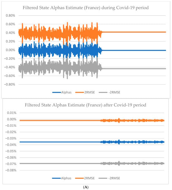
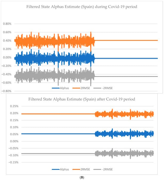
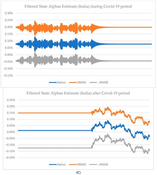
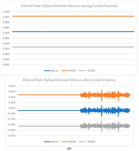
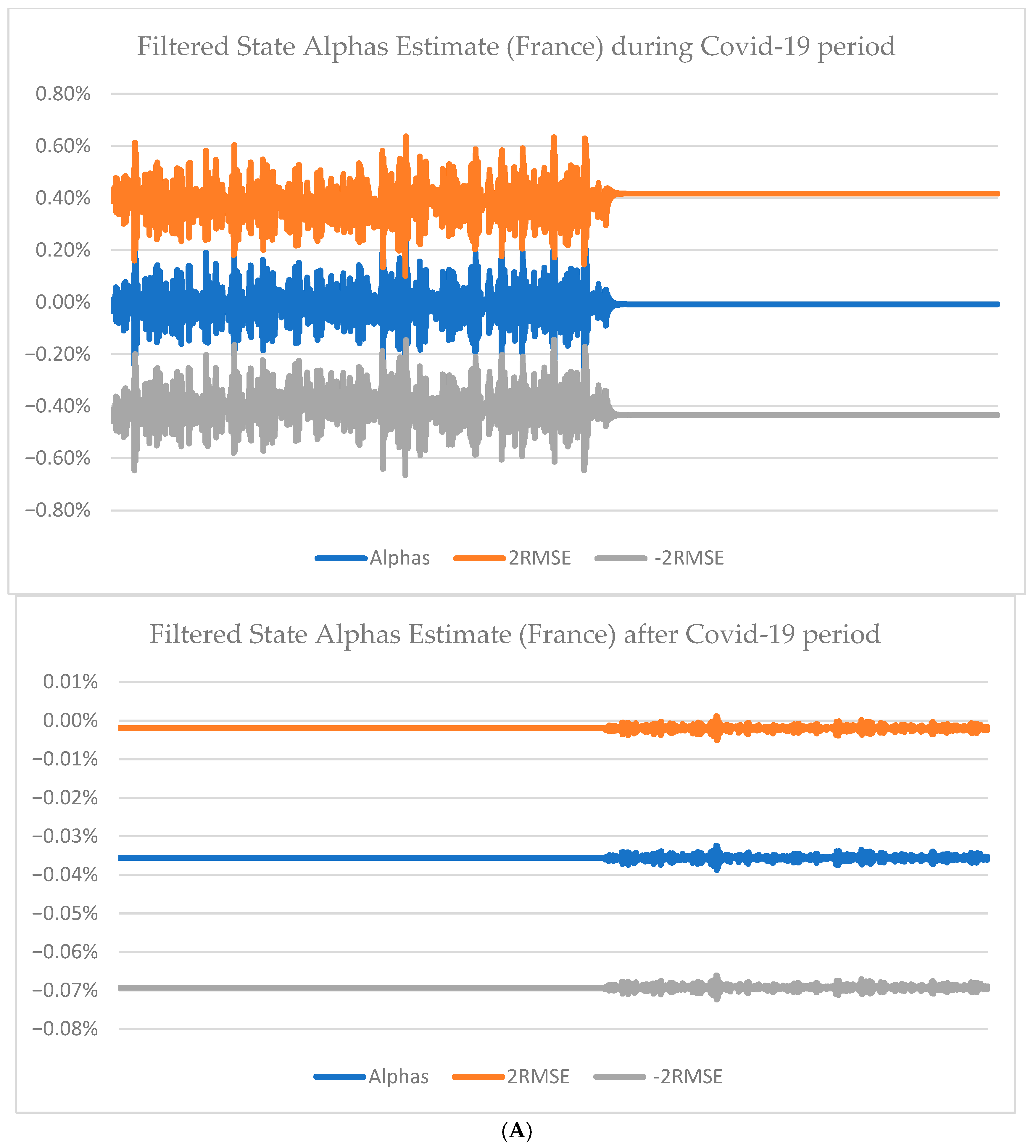
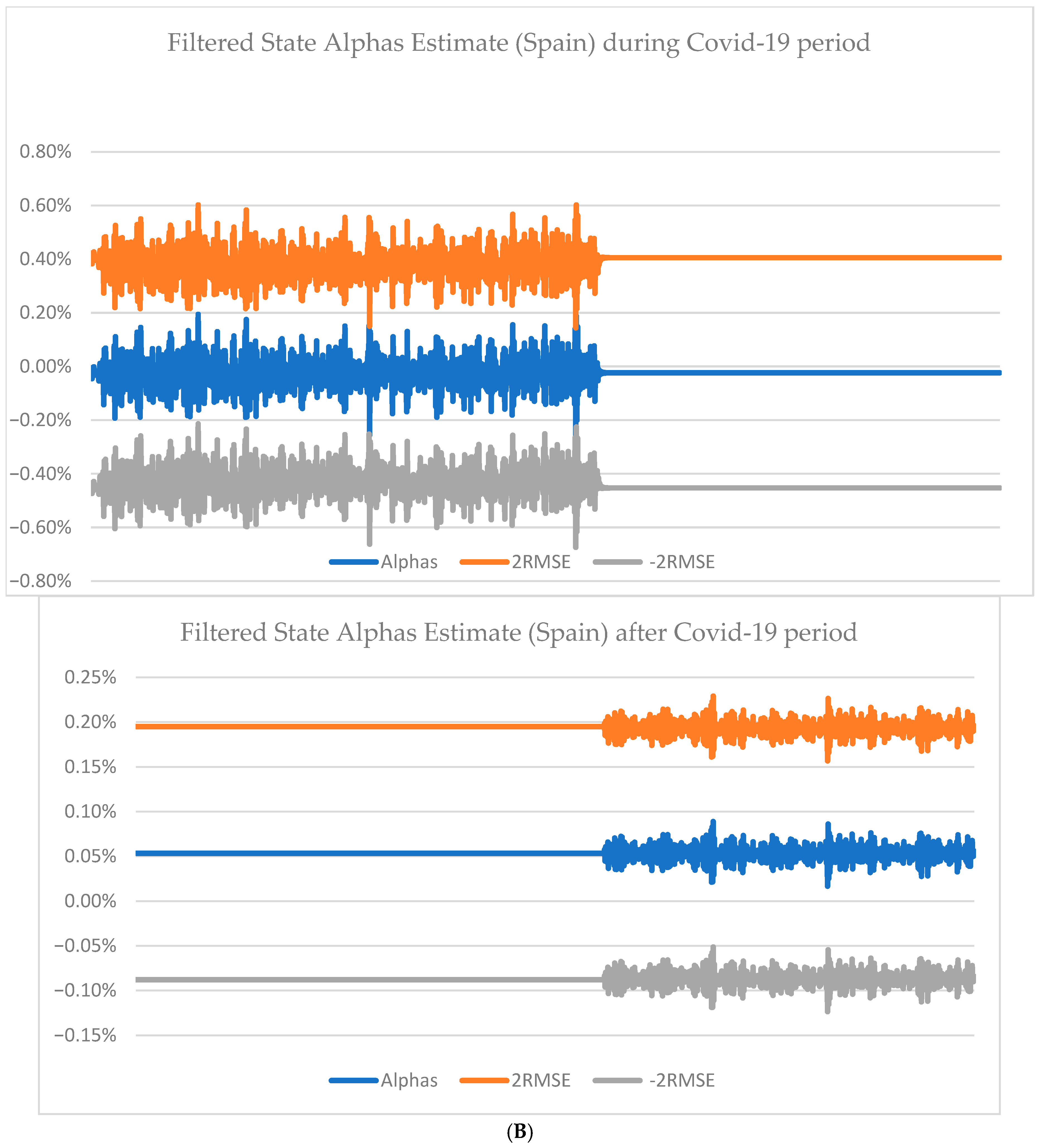
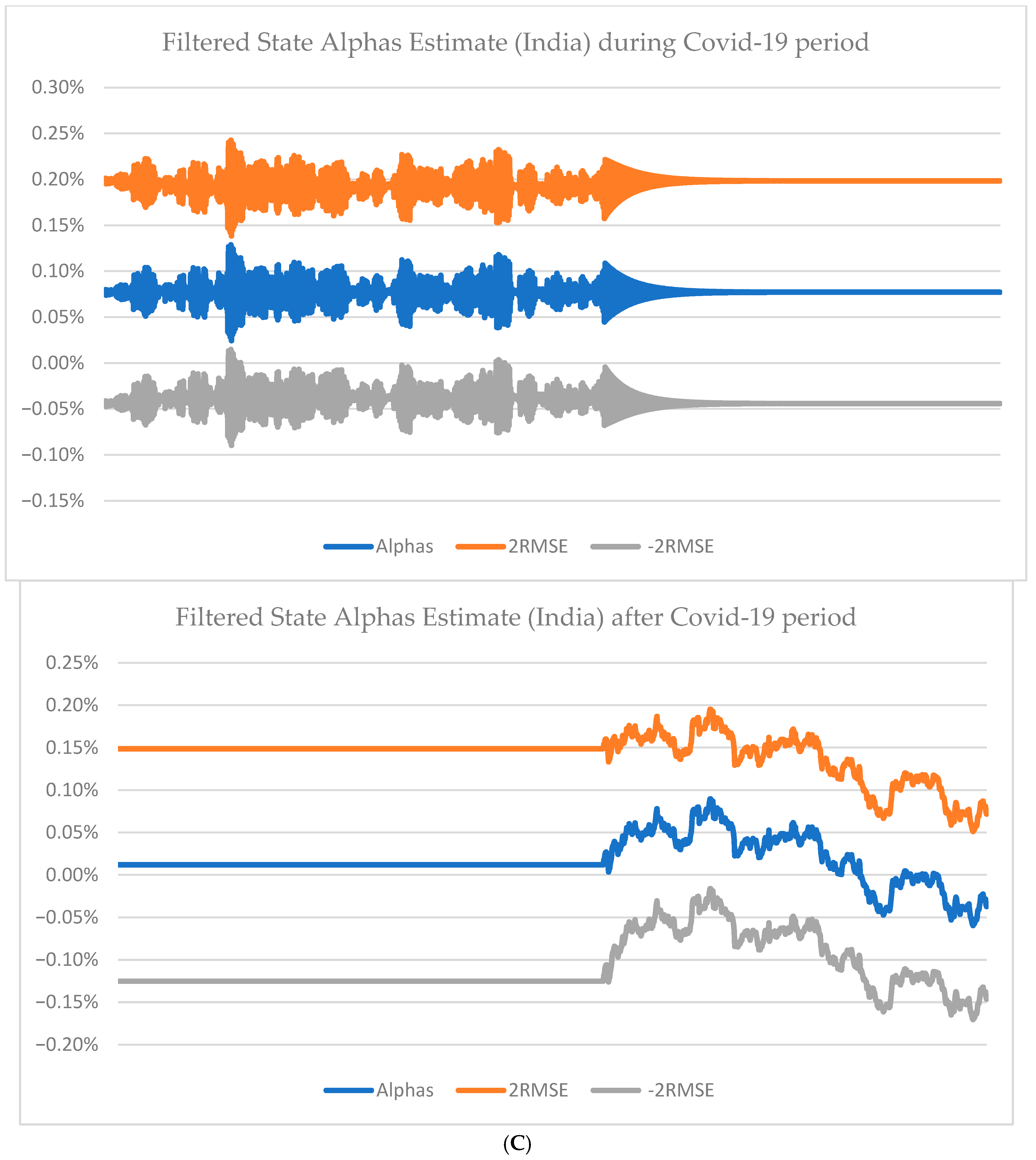
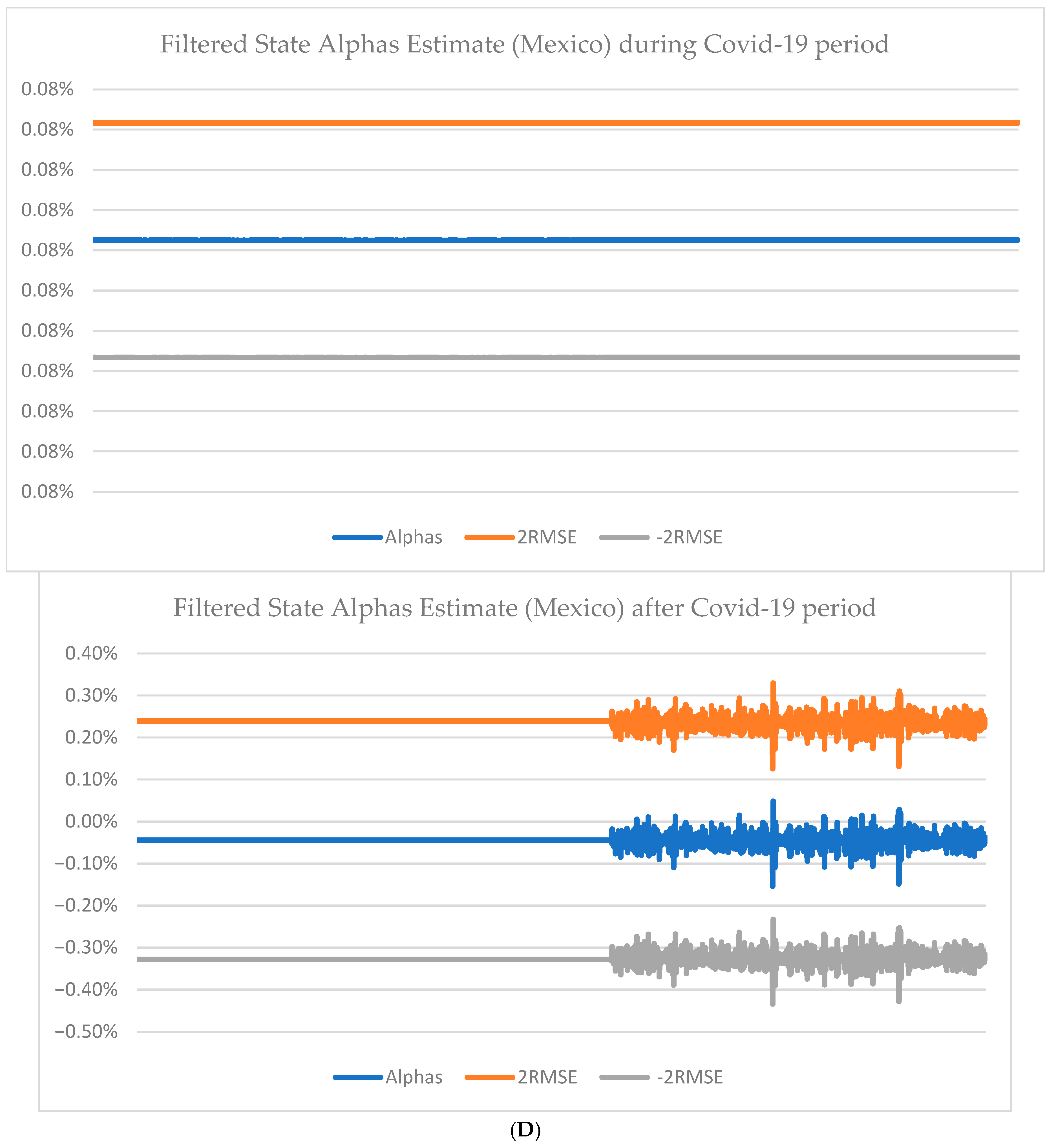
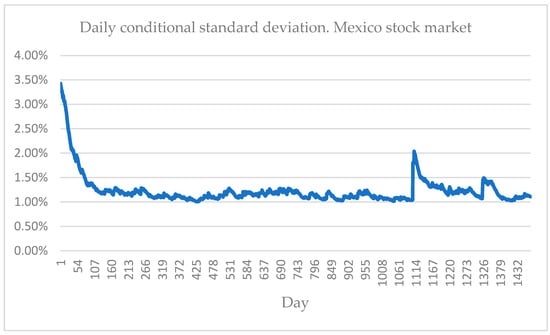

Disclaimer/Publisher’s Note: The statements, opinions and data contained in all publications are solely those of the individual author(s) and contributor(s) and not of MDPI and/or the editor(s). MDPI and/or the editor(s) disclaim responsibility for any injury to people or property resulting from any ideas, methods, instructions or products referred to in the content. |
© 2026 by the authors. Licensee MDPI, Basel, Switzerland. This article is an open access article distributed under the terms and conditions of the Creative Commons Attribution (CC BY) license.