


Abstract
Global value chains can diversify risk, but they can also transmit production disruptions and financial losses across interconnected economies. This study examines whether trade–finance coupling amplifies systemic loss relative to a trade-only benchmark, how diversification-based risk sharing offsets that amplification, and whether multilayer structure changes systemic rankings. We develop a transparent multilayer stress-testing framework linking trade–value–chain dependence, reconstructed foreign currency portfolio exposures, and cross-layer shock transmission for 20 country-sector nodes. The trade layer is based on 2014 WIOD data, while 2023 CPIS foreign currency asset margins are allocated using relative entropy; 5000 common and idiosyncratic shock simulations are evaluated across alternative propagation and absorption regimes. Mean output-weighted loss increases from 1.009% under trade-only propagation to 1.379% in the baseline multiplex model, while the 95th percentile rises from 5.092% to 6.217%. Eliminating diversification-based absorption raises mean loss to 1.541%, whereas stronger absorption lowers it to 1.251%. Robustness checks using alternative financial scaling and a 12-node aggregation preserve the main qualitative result. These calibrated stress-test outcomes, rather than causal or historical estimates, show that the balance between risk sharing and contagion is benchmark- and state-dependent.
1. Introduction
The globalization of production has replaced a large share of arm’s length exchange in final goods with dense systems of intermediate production, contractual specialization, and cross-border financing. A modern export typically embodies inputs, services, intellectual property, and working capital from several jurisdictions. This fragmentation raises productivity by permitting firms to exploit comparative advantage at finer stages of production, but it also means that a disruption originating in one country-sector can become an input shortage, a liquidity problem, and a balance sheet loss elsewhere. The central policy question is therefore no longer whether trade and finance transmit shocks. It is whether the same connections that permit diversification and risk sharing become destabilizing when their topology overlaps (Baldwin 2016; Antràs 2020; World Bank 2020; Hummels et al. 2001; Johnson and Noguera 2012; Koopman et al. 2014; Timmer et al. 2014; Los et al. 2015).
Two analytical traditions address parts of this question. The production network literature shows that idiosyncratic shocks need not wash out when input–output linkages are asymmetric, concentrated, or characterized by low substitution (Acemoglu et al. 2012; Carvalho 2014; Gabaix 2011; Baqaee and Farhi 2019; Barrot and Sauvagnat 2016; Boehm et al. 2019; Carvalho et al. 2021; Inoue and Todo 2019; Bonadio et al. 2021; Pichler et al. 2022). The financial network literature shows that claims among banks, investors, firms, and sovereigns can disperse losses in normal times but create contagion, fire sales, and common exposure effects under stress (Allen and Gale 2000; Eisenberg and Noe 2001; Gai and Kapadia 2010; Battiston et al. 2012; Elliott et al. 2014; Acemoglu et al. 2015; Glasserman and Young 2016; Haldane and May 2011; Billio et al. 2012; Diebold and Yılmaz 2014; Bargigli et al. 2015; Poledna et al. 2015; Aldasoro and Alves 2018). Yet production and finance are usually assessed separately. That separation is increasingly difficult to defend. A supplier’s failure can reduce a customer’s output and cash flow; the customer’s deterioration can then revalue loans and securities held by institutions that also finance other firms in the same production cluster. Conversely, diversified foreign investment can smooth a localized production shock by transferring income across borders, provided that liquidity remains available and portfolios are not exposed to the same impaired nodes.
This paper develops a multilayer trade finance framework in which the same country-sector nodes occupy three analytically distinct layers. The trade–value–chain layer records the dependence of a customer sector on upstream intermediate suppliers. The financial exposure layer records the vulnerability of an investor node to distress at foreign issuer nodes. A third layer captures sequential paths in which a shock moves from production to finance or from finance to production. The layers are combined in a linear stress engine whose stability is governed by its spectral radius. Risk sharing enters as node-specific absorption proportional to the entropy of trade suppliers and financial counterparties. This construction makes it possible to ask not only which nodes are central, but which ones transmit the greatest output-weighted loss, which receive the greatest average distress, and how much the financial layer adds after diversification is taken into account.
The empirical exercise is intentionally reproducible and conservative. The trade layer uses a publicly available aggregation of the 2014 World Input-Output Database (WIOD) into four regions—the United States, Canada, Mexico, and the rest of the world—and five sectors—agriculture, resources, transport equipment, other manufacturing, and services. The financial layer uses 2023 Coordinated Portfolio Investment Survey (CPIS) assets denominated in currencies other than the reporting economy’s domestic currency. The public series used here supplies reporting economy margins but not the complete bilateral country-sector claims needed by the model. The missing bilateral matrix is therefore reconstructed using an entropy-consistent allocation with an observed trade-prior and destination output weights. The reconstruction preserves observed CPIS source margins in dollar levels. Importantly, the baseline propagation operator subsequently normalizes each investor row. The source margin scale therefore cancels from the transition probabilities: the CPIS data constrain the level matrix and exposure composition, whereas β is a stress design coefficient governing the strength of financial transmission. This distinction is made explicit so that the reconstructed financial layer is not interpreted as an empirically estimated mapping from portfolio dollars to propagated distress.
The use of different trade and financial vintages also requires precision. This paper does not claim to estimate a contemporaneous 2014 or 2023 causal system. Instead, it overlays a benchmark global production topology with the latest common financial margin year available for the three individually represented North American economies in the selected CPIS series. The resulting exercise is a two-vintage structural stress test. Its purpose is to identify mechanisms, rankings, and sensitivity—not to forecast realized GDP losses or assign default probabilities to specific firms, countries, or sectors.
To discipline the scope, this paper adopts a hierarchical research design. The primary research question is whether adding financial and cross-layer transmission to a fixed production network materially changes system-wide loss relative to a trade-only benchmark. The first subordinate question concerns mechanism: under what combinations of diversification, liquidity, shock correlation, and propagation strength does risk-sharing absorption offset—or fail to offset—the additional contagion channels? The second subordinate question is diagnostic: does a multilayer stress measure identify systemically important nodes that would be missed or misranked by single-layer centrality or trade-only propagation? Policy implications are treated as consequences of these three analytical questions rather than as a separate research objective.
Four findings emerge. First, trade and finance are related but not redundant. Their node centralities have a Spearman rank correlation of 0.523, while the Jaccard overlap of strong directed edges is only 0.118. Second, adding financial and cross-layer propagation increases both average and tail loss. Across 5000 common and idiosyncratic draws, the mean system loss rises from 1.009% in the trade-only model to 1.379% in the baseline multiplex model, and the 95th percentile rises from 5.092% to 6.217%. Third, diversification materially absorbs contagion: eliminating risk-sharing absorption raises mean loss to 1.541%, whereas stronger absorption lowers it to 1.251%. Fourth, the financial layer changes the identity of important nodes. Rest-of-world services and manufacturing remain dominant because of their output size and production centrality, but Canadian services move sharply upward because reconstructed foreign currency exposure creates an additional transmission channel. Additional robustness checks leave the main qualitative result unchanged: an expanded α − γ grid, variation in the probability of common sectoral shocks, a CPIS scale-sensitive financial operator, and a 12-node alternative aggregation all preserve the benchmark distinction between trade-only and multiplex propagation. In the 12-node aggregation, baseline mean loss is 1.371% and P95 loss is 6.187%, compared with 1.379% and 6.217% in the 20-node system, and the ranking of the 12 comparable broad region-sector transmitters is unchanged (Spearman ρ = 1.000).
The incremental contribution lies in what the joint framework reveals rather than in the mere existence of a multilayer model. First, it distinguishes two counterfactuals that are often conflated: finance can be stabilizing relative to a multiplex system with no risk sharing while remaining destabilizing relative to a trade-only system. Second, it shows that the balance is state-contingent: greater absorption reduces loss, whereas stronger financial and cross-layer transmission together with weaker liquidity buffers move the system toward higher feedback amplification. Third, it separates topological importance from stress-based marginal contribution, so multilayer information can alter systemic rankings even when single-layer centralities are positively correlated. These results refine the conventional diversification-versus-contagion dichotomy by making the sign of integration benchmark-dependent and state-dependent. The contribution is therefore theoretical-mechanistic and calibration-based rather than causal or historical.
The remainder of the paper proceeds as follows. Section 2 reviews the literature on global value chains, production networks, international risk sharing, and financial contagion, and states the paper’s structural propositions. Section 3 documents the data and the status of observed versus reconstructed quantities. Section 4 presents the multilayer model, systemic indicators, scenarios, and robustness design. Section 5 reports the network topology, node rankings, scenario results, Monte Carlo tail losses, and sensitivity analyses. Section 6 and Section 7 discuss interpretation and policy implications. Section 8 sets out the limitations and a research agenda. Section 9 concludes the paper.
2. Literature Review and Analytical Propositions
2.1. Global Value Chains as Mechanisms of Specialization and Risk Sharing
Global value chains (GVCs) permit production stages to be located where capabilities, costs, institutions, and market access are most favorable. Vertical specialization measures the foreign content embodied in exports, while value-added trade accounting separates domestic contribution from gross border crossings (Hummels et al. 2001; Johnson and Noguera 2012; Koopman et al. 2014; Timmer et al. 2014; Los et al. 2015). This distinction matters for systemic risk. A country can appear highly exposed in gross trade while retaining only a small share of the value added, or appear diversified across export destinations while depending on a narrow set of foreign intermediate inputs. Input–output data are therefore better suited than gross bilateral trade alone to identify the channels through which production shocks travel.
The risk-sharing case for integration follows from standard international macroeconomics. Ownership of foreign claims can separate national income from national production, permitting consumption to be smoothed after country-specific disturbances (Obstfeld 1994; Backus et al. 1992; Kose et al. 2009; Imbs 2006). In a complete-markets benchmark, residents diversify claims on domestic output and share risk internationally. Real-world portfolios are incomplete and home biased, but cross-border equity, debt, and bank claims still create channels for income insurance. From this perspective, a financial layer linked to GVCs can be stabilizing: losses in one production node are partially borne by geographically dispersed investors, while credit lines and trade finance can bridge temporary working capital gaps.
The same mechanism has a state-contingent weakness. Risk sharing depends on the solvency and liquidity of intermediaries, on the heterogeneity of portfolios, and on the absence of coordinated deleveraging. When investors hold similar claims, diversification at the individual level may create common exposure at the system level. When collateral values fall, or funding is withdrawn, a network that spreads risk ex ante can accelerate distress ex post. The relevant distinction is thus not between connected and disconnected systems, but between connections that diversify independent shocks and connections that align losses under common stress.
2.2. Production Networks and Shock Propagation
Input–output networks provide a natural representation of technological dependence. Leontief’s accounting system maps final demand into gross output through the inverse of the technical coefficient matrix (Leontief 1936; Miller and Blair 2009). Modern network macroeconomics adds heterogeneity in node size, centrality, substitution, and propagation. Aggregate volatility can emerge from microeconomic shocks when large or central suppliers have disproportionate influence (Acemoglu et al. 2012; Carvalho 2014; Gabaix 2011; Baqaee and Farhi 2019). Higher-order production linkages matter because a disruption to one input can affect customers, their customers, and eventually final demand. The resulting multiplier is determined by both the intensity and the direction of intermediate use.
Empirical evidence from earthquakes, floods, and the COVID-19 pandemic confirms that supply chain relationships transmit shocks beyond directly affected firms and regions (Barrot and Sauvagnat 2016; Boehm et al. 2019; Carvalho et al. 2021; Inoue and Todo 2019; Bonadio et al. 2021; Pichler et al. 2022; Baqaee and Farhi 2020). The magnitude depends on input specificity, inventories, alternative suppliers, adjustment costs, and the duration of the disruption. A purely linear input–output model can overstate losses when substitution is easy and understate them when bottleneck inputs are essential. Nevertheless, linear network models remain valuable as transparent stress-testing devices, particularly when their parameters are interpreted as exposure weights rather than immutable technologies.
The global input–output network is also modular (Cerina et al. 2015). Country-sector communities emerge from geography, trade agreements, industrial specialization, and regional production systems (Dietzenbacher et al. 2013; Timmer et al. 2015). Communities may contain shocks locally when they have redundant external links, but they may also concentrate risk when several members depend on a common upstream supplier. The distinction between transmitter and receiver centrality is therefore essential. A node can be highly vulnerable to incoming shocks without generating large system-wide losses when it is itself impaired; conversely, a large supplier can be a major transmitter while remaining relatively resilient to disturbances elsewhere.
2.3. Financial Networks, Common Exposure, and Contagion
Financial networks have long been understood to generate a robust-yet-fragile trade-off. Interbank and portfolio claims diversify bilateral counterparty losses, but they also create paths for default contagion and valuation spillovers (Allen and Gale 2000; Eisenberg and Noe 2001; Gai and Kapadia 2010; Battiston et al. 2012; Elliott et al. 2014; Acemoglu et al. 2015; Glasserman and Young 2016). In clearing models, payment shortfalls propagate through liabilities. In mark-to-market and fire-sale models, losses propagate before default because institutions sell common assets, tighten credit, or breach leverage constraints. Measures such as DebtRank, network centrality, and variance–decomposition connectedness quantify different aspects of this dependence (Elliott et al. 2014; Billio et al. 2012; Diebold and Yılmaz 2014).
Topology changes the result. Dense networks may absorb small shocks because losses are spread widely, but may transmit large shocks to many counterparties once buffers are exhausted. Core-periphery structures concentrate systemic importance in a small set of intermediaries. Multiplex representations add the fact that the same institutions are connected through unsecured credit, securities, derivatives, foreign exchange, and overlapping portfolios (Haldane and May 2011; Bargigli et al. 2015; Poledna et al. 2015; Aldasoro and Alves 2018; Montagna and Kok 2016; Kivelä et al. 2014; Boccaletti et al. 2014). Aggregating these layers can conceal vulnerabilities because exposures that appear diversified in one market may be concentrated across the system.
Cross-border finance adds currency and jurisdictional dimensions. International portfolios can insure domestic income, but foreign currency positions are sensitive to exchange rates, global funding conditions, and safe-asset demand. Global banks transmit monetary and liquidity shocks through internal capital markets and cross-border lending (Lane and Milesi-Ferretti 2007; Forbes and Chinn 2004; Cetorelli and Goldberg 2012; Kalemli-Ozcan et al. 2013). A GVC firm may therefore face a joint shock: reduced orders or missing inputs on the real side and tighter credit or revaluation losses on the financial side. A multilayer framework is needed to represent this joint exposure.
2.4. Multilayer Integration and Structural Propositions
Multilayer network theory distinguishes relationships by type while preserving a common node set (De Domenico et al. 2013; Newman 2010; Kivelä and Porter 2018). This is preferable to collapsing all exposures into one adjacency matrix because a trade edge and a portfolio edge carry different economic meanings, directions, and loss mechanisms. Interlayer paths are especially important: a production shock can weaken an issuer and impair investors; an investor loss can reduce credit and amplify production constraints. The present model captures these sequences through products of layer-specific transition matrices.
Recent research has begun to bridge production and financial contagion more directly. Tabachová et al. (2024) use firm-level supply relationships and bank loans to show that supply chain contagion can materially amplify financial losses; Fialkowski et al. (2026) develop an econo-financial stress-testing framework linking firm-level supply chains, bank-firm credit, and interbank exposures; and Chae and Inoue (2026) integrate cross-border financial exposures with international trade linkages in a country-level multilayer contagion model. Relative to these studies, the present framework focuses on country-sector global value chain dependence, reconstructs a foreign currency portfolio layer from observed source margins under transparent entropy constraints, models diversification explicitly as a risk-sharing absorption mechanism, and compares trade-only, multiplex, and liquidity-stress regimes using identical Monte Carlo shock draws. The objective is therefore complementary: a reproducible structural stress test of how risk sharing and contagion coexist when production and portfolio channels overlap.
The analysis is organized around four structural propositions. Proposition 1 is non-redundancy: trade and financial centrality rankings should be positively associated because large economies and sectors are important in both layers, but the association should be imperfect because production dependence and foreign currency portfolio exposure are distinct. Proposition 2 is multiplex amplification: holding direct shocks constant, adding financial and cross-layer paths should increase mean and tail system losses relative to a trade-only benchmark. Proposition 3 is conditional risk sharing: greater diversification should lower propagation by distributing shocks and increasing absorption, but may not fully offset the additional channels introduced by finance. Proposition 4 is ranking instability: nodes with modest trade-only impact can become systemically important when financial exposure is included.
The propositions also have an explicit hierarchy. Multiplex amplification is the primary proposition because it answers the central counterfactual question. Conditional risk sharing identifies the countervailing mechanism that can attenuate that amplification. Non-redundancy and ranking instability are diagnostic implications of the multilayer representation: they matter because they show when the additional layer changes what the analyst sees, not because centrality comparison is an independent objective.
These propositions are not conventional causal hypotheses tested on repeated historical crises. They are model-implied statements evaluated within a calibrated stress-testing environment. Their value lies in disciplined comparison across regimes using the same direct shock draws and the same observed production accounts.
3. Data and Network Construction
3.1. World Input–Output Data
The production layer is built from the 2014 WIOD release as transformed by a publicly reproducible aggregation program (World Input-Output Database 2016). The source world input–output table contains 43 countries, a rest-of-world aggregate, and 56 industries. The replication transformation used here aggregates those observations to four regions and five sectors. The four regions are the United States, Canada, Mexico, and the rest of the world. The five sectors are agriculture (A), resource extraction (R), transport equipment, including motor vehicles and other transport equipment (T), other manufacturing (M), and services (S). The resulting 20-industry system preserves intermediate transactions, consumption and investment final demand for each region, value added, and gross output accounting totals.
Let Z be the 20 × 20 matrix of intermediate transactions, where Zij is output from supplier i used by customer j. Let f be the vector of final demand and x gross output. The data satisfy x = Z1 + f by rows and x = Z′1 + v by columns, where v is value added. The maximum numerical discrepancy in the supplied table is 2.84 × 10⁻¹⁴ for the row identity and 6.99 × 10⁻⁷ for the column identity, the latter reflecting text file rounding. The spectral radius of the technical coefficient matrix is 0.595, safely below unity, so the Leontief inverse exists.
This aggregation is coarse relative to the full WIOD, but it is useful for a transparent article-scale stress test. It retains the North American production system as separate economies, distinguishes transport equipment from other manufacturing, and embeds all remaining countries in a rest-of-world block. The cost is substantial: heterogeneity within the rest-of-world aggregate is suppressed, bilateral bottlenecks inside that block cannot be identified, and the 77.23% output share of the rest-of-world mechanically affects absolute impact and community structure. The resulting community assignments and node rankings are therefore conditional diagnostics of the 20-node representation, not empirical claims that the same ordering would survive full WIOD or OECD ICIO disaggregation. As an aggregation-sensitivity check, the analysis also combines agriculture with resources and transport equipment with other manufacturing, producing a 12-node, three-sector-per-region system. Aggregate mean and tail losses remain close to the 20-node results, and the 12 comparable broad-group transmitter ranks are identical (Spearman ρ = 1.000). This coarser alternative supports robustness to the particular five-sector split, but it does not substitute for a materially finer WIOD/OECD ICIO rerun before granular rankings are interpreted externally.
3.2. CPIS Foreign Currency Portfolio Margins
The financial calibration uses the IMF Coordinated Portfolio Investment Survey indicator “Assets, Total Investment, Denominated in Other Currencies” in US dollars, retrieved through the World Bank Data360 interface (International Monetary Fund 2018, 2026; World Bank 2026). The selected 2023 cross-section contains non-missing observations for 50 reporting economies. It records total portfolio assets denominated in currencies other than the reporting economy’s domestic currency against the world counterpart. It is not a measure of all foreign portfolio assets, bank loans, foreign direct investment, derivatives, or trade credit. The interpretation throughout the paper is therefore deliberately narrow: it is a foreign currency portfolio exposure margin.
The United States margin is USD 115.740 billion, Canada USD 257.172 billion, and Mexico USD 70.365 billion. The sum for all other reporting economies is USD 2.460 trillion, producing a four-region total of USD 2.903 trillion. The rest-of-world value is large partly because that aggregate includes financial centers and all reporting economies other than the three separately represented countries. CPIS participation and coverage are not complete, so the margins are lower-bound reported positions rather than a census of global foreign currency assets.
The financial and trade years do not match; 2023 is the only year in the selected public indicator for which the United States, Canada, and Mexico all have non-missing positive observations, whereas the reproducible aggregated WIOD table is for 2014. The model is consequently a structural overlay of a 2014 production topology and 2023 financial margins. This design is appropriate for mechanism-based stress testing but not for historical attribution.
3.3. Observed, Reconstructed, and Simulated Quantities
Table 1 separates the empirical status of each component. This distinction is central to the credibility of the exercise. Observed input–output transactions and CPIS source margins enter the dollar-valued reconstruction directly. Bilateral financial exposures are reconstructed because the selected public series does not contain the required country-sector matrix. In the baseline row-normalized financial operator, CPIS source margins do not scale row-specific transition intensity; β remains a calibrated stress parameter. To assess whether the normalization influences the results, the analysis also considers a CPIS scale-sensitive specification in which each investor row is multiplied by the reporting region’s observed CPIS asset share relative to its WIOD gross output share. Propagation coefficients and shock distributions remain scenario inputs, so all reported losses are conditional model outcomes rather than directly observed losses. Table 2 documents the region–sector aggregation, Table 3 reports the 2023 regional CPIS margins, and Figure 1 summarizes the empirical and analytical architecture of the framework.
Table 1.
Data sources, transformations, and empirical status.
Table 2.
Region–sector aggregation.
Table 3.
2023 CPIS foreign currency portfolio exposure margins used in the financial layer.
Figure 1.
Empirical and analytical architecture of the multilayer trade finance framework.
Accordingly, the results are interpreted at three distinct evidentiary levels. Aggregate system loss comparisons are calibrated stress-test outputs; topology and community statistics are descriptive properties of the chosen aggregation; and node-level financial increments are illustrative, reconstruction-dependent diagnostics rather than empirical estimates of bilateral exposure or realized loss. This distinction is repeated where the corresponding results are discussed so that numerical precision is not mistaken for empirical identification.
4. Methodology
4.1. Trade–Value–Chain Layer
The technical coefficient matrix A is obtained by dividing each intermediate purchase by the gross output of the purchasing node. Thus gives the amount of input i required per unit of output j. The Leontief quantity system is x = Ax + f, so x = (I − A)−1f. For final demand validation exercises, a negative change Δf produces Δx = (I − A)−1Δf. The Leontief multiplier reported for each scenario is the ratio of total gross output change to the direct final demand change.
The shock propagation trade matrix differs from A because the stress engine is expressed as distress transmitted from a supplier to a customer. For customer j, the weight assigned to supplier i is the share of j’s total intermediate purchases obtained from i. Self-dependence is removed, and the remaining weights are renormalized. If hi is distress at supplier i, the trade contribution to next-round distress at customer j is proportional to Tjihi. This orientation makes every row of T a customer’s distribution of upstream exposure.
4.2. Financial Exposure Layer and Relative-Entropy Reconstruction
Let ar denote the observed CPIS foreign currency asset margin for reporting region r. The objective is to allocate ar across foreign destination regions q without claiming access to unobserved bilateral holdings. The prior combines the observed cross-border trade flow from r to q and destination q’s share of gross output. Specifically, 85% of the prior weight is based on the source region’s trade allocation and 15% on destination size. Domestic claims are excluded. With only a source margin constraint, minimizing the Kullback–Leibler divergence from this normalized prior yields Frq = arprq. This is the relative-entropy solution closest to the prior subject to the observed row total (Squartini et al. 2018; Cimini et al. 2015; Anand et al. 2015).
To make the prior in Equation (3) dimensionally coherent, the cross-border trade component is first converted into a source-specific distribution over eligible foreign destinations, and destination gross output is likewise converted into a foreign destination output share. Both components are therefore dimensionless, and each sums to one over eligible foreign destinations before the 85/15 mixture is formed.
Country-level reconstructed claims are allocated to sectors by the gross output shares of source and destination sectors. If sir is the output share of source sector i within region r and djq the output share of destination sector j within q, then the claim from source node i to destination node j is Fij = Frqsirdjq. This allocation preserves every observed region-level source margin exactly. A pure-entropy robustness case replaces the trade component of the prior with destination size alone.
Propagation follows the asset-loss direction. If investor node i holds claims on issuer node j, distress at j affects i. The normalized financial transition weight is therefore the claim Fij divided by investor i’s total reconstructed foreign exposure. Every investor row sums to one before scaling by the financial propagation parameter. We reserve F exclusively for the dollar-valued reconstructed claims matrix and denote the row-normalized financial transition matrix by W. The symbol W is used consistently in all subsequent propagation, cross-layer, and diversification expressions.
An important algebraic implication of this normalization is that the CPIS source amount cancels from the transition weights. For an investor node i in reporting region r, the reconstructed row sum equals the region-level source margin allocated to that investor, . Dividing each bilateral claim by that row sum therefore removes both ar and the source sector scale, leaving only the within-row destination allocation. The baseline financial operator is consequently a conditional exposure share matrix: it identifies where an investor is exposed, not how large the investor’s total foreign currency balance sheet is. The observed CPIS margins remain essential for the reconstructed dollar matrix and any level-based exposure diagnostic, but they do not by themselves increase a row’s propagation strength. Accordingly, β must be interpreted as an assumed financial stress-transmission coefficient rather than an elasticity estimated from CPIS amounts. This clarification separates empirical level information from scenario propagation intensity.
To make the role of observed exposure amounts testable rather than merely interpretive, an additional scale-sensitive robustness operator is defined as Wscale = E W, where the diagonal element for an investor in region r is er = (ar/Σq aq)/(xr/Σq xq). This dimensionless ratio compares the region’s share of reported CPIS foreign currency assets with its share of WIOD gross output; its output-weighted regional mean is one, so the system-wide scale of β remains centered on the baseline while row-specific financial transmission varies with observed relative exposure. The implied factors are 0.206 for the United States, 4.347 for Canada, 1.817 for Mexico, and 1.097 for the rest of the world. This mapping is a transparent robustness design, not an estimated balance sheet elasticity. In the CPIS scale-sensitive robustness calculation, the cross-layer matrix is recomputed from the scaled financial operator before constructing the propagation matrix. The diversification scores, and therefore the absorption matrix D(φ), are held at their baseline values because the regional scale factor multiplies every counterparty exposure in a given investor row proportionally and hence leaves the normalized within-row shares—and their Shannon entropy—unchanged.
prq ∝ 0.85 · Traderq + 0.15 · OutputShareq, prr = 0
Frq = arprq, Fij = Frqsirdjq
4.3. Cross-Layer Paths and Risk-Sharing Absorption
Sequential propagation is represented by the normalized average of TW and WT. The product TW captures a financial transmission followed by an input dependence transmission under the matrix orientation used here; WT captures the reverse sequence. These paths are not additional observed claims. They summarize second-order routes that would be missed if trade and finance were simply added without interaction.
Risk sharing is represented as node-specific absorption. For each node, normalized Shannon entropy is computed over its upstream trade weights and financial counterparty weights (Shannon 1948). The average of the two entropies is the diversification score di. A node with exposure spread across many similarly weighted counterparties has a score closer to one; a concentrated node has a lower score. The diagonal absorption matrix is D(φ) = diag(1 − φdi), where φ controls how strongly diversification reduces incoming propagation. This formulation does not assume that diversification prevents direct losses. It reduces only the feedback transmitted through the network.
For each row, Shannon entropy is calculated over the positive normalized exposure weights and divided by the natural logarithm of the number of positive counterparties in that layer; rows with a single positive counterparty are assigned zero normalized entropy. This places each layer-specific entropy on the unit interval before the trade and financial components are averaged.
The baseline propagation matrix is P = D(φ)(αT + βW + γC), where C is the cross-layer matrix. Parameters α, β, and γ determine the strength of trade, finance, and sequential cross-layer transmission. The baseline values are α = 0.32, β = 0.14, γ = 0.08, and φ = 0.20. The resulting spectral radius is 0.479, below unity, so the infinite feedback series converges. A direct shock vector s produces total distress h = (I − P)−1s. Values are capped at one for simulation outputs, although the selected baseline parameters rarely approach that bound outside the shocked node.
P = D(φ)(αT + βW + γC), h = (I − P)−1s
4.4. Systemic Importance, Vulnerability, and Communities
Systemic transmitter impact is measured by shocking each node by 10% and computing the output-weighted total distress. This metric incorporates node size and all higher-order propagation paths. The trade-only counterpart sets β = γ = 0. The financial increment is the difference between baseline multiplex impact and trade-only impact. The risk-sharing benefit is the difference between multiplex impact with φ = 0 and the baseline with φ = 0.20.
Receiver vulnerability is the expected distress of each node under equally likely 10% shocks at every node. It is therefore a row-based measure of exposure to the rest of the system, distinct from transmitter impact. PageRank and weighted betweenness are reported as topological diagnostics, but the paper gives priority to stress-based impact because centrality alone does not account for node size, layer parameters, or absorption.
Communities are identified in the symmetrized weighted multiplex network using greedy modularity maximization. This procedure is descriptive. It indicates whether country-sector groups are more strongly connected internally than externally, but it does not establish optimal currency areas, legal groups, or causal blocs.
4.5. Stress Scenarios and Monte Carlo Design
Five deterministic scenarios are considered: a 10% shock to United States services; a 10% disruption to rest-of-world manufacturing; a 10% shock to Mexican transport equipment; a 10% shock to Canadian resources; and a correlated 5% shock to transport equipment in all four regions. Each scenario is evaluated under five regimes. The trade-only regime excludes finance and cross-layer paths. The no-sharing multiplex regime sets φ to zero. The baseline uses the parameters above. Strong risk sharing doubles φ to 0.40. The tight liquidity regime raises α, β, and γ to 0.34, 0.24, and 0.12 while reducing φ to 0.10.
Parameter selection follows a stress design logic rather than statistical estimation. The baseline trade weight α = 0.32 gives the production channel the largest direct propagation role; the finance weight β = 0.14 assigns a smaller role to the narrower foreign currency portfolio layer; the cross-layer weight γ = 0.08 keeps sequential transmission below either direct layer; and the absorption coefficient φ = 0.20 represents partial rather than complete diversification-based attenuation. The tight liquidity regime deliberately raises propagation weights and reduces absorption, so its position as the high-loss regime is partly encoded by construction. These coefficients are used to generate economically interpretable comparative statics under a stable propagation matrix and should not be read as estimated elasticities, historical crisis coefficients, or structural parameters identified from data.
The Monte Carlo exercise uses 5000 common random shock vectors, reused across regimes. With probability 0.78, a single node is selected uniformly and receives a severity between 4% and 22%, generated from a scaled beta distribution. With probability 0.22, one sector is selected, and all four regional nodes receive correlated severities generated from a common beta draw and lognormal dispersion, capped at 20%. This mixture creates both idiosyncratic disruptions and common sectoral shocks. Reported statistics are the mean, median, 95th percentile, expected shortfall above the 95th percentile, and the cascade multiplier relative to the direct output-weighted shock. The complete distributional parameterization is reported in Appendix B (Table A3).
The distributions are model-based, not sampling distributions. Consequently, no frequentist confidence intervals are attached to the simulated losses. Reproducibility is achieved by fixing the random seed and releasing every shock draw and regime outcome.
For exact replication, Appendix B reports the beta-shape parameters, the lognormal dispersion parameter, the mixture probabilities, the severity transformations, and the fixed random seed. The same realized 5000 shock vectors are reused across propagation regimes, while the released shock-draw file and analysis scripts provided in the Supplementary Materials allow executable replication of the generator and reported simulations.
4.6. Robustness and Validation
Seven robustness and validation exercises are used in the analysis. First, financial propagation β ranges from 0.05 to 0.30 and absorption φ from 0 to 0.50 in the original 36-cell grid. Second, trade propagation α is varied from 0.20 to 0.44 jointly with cross-layer propagation γ from 0 to 0.16. Third, the probability of a common sector-wide shock is varied from 0 to 0.60 while retaining the same shock-severity laws and random seed. Fourth, the trade-prior financial reconstruction is compared with the pure-entropy destination size reconstruction. Fifth, the CPIS scale-sensitive financial operator defined above is compared with the row-normalized baseline. Sixth, the production and financial networks are re-aggregated from five to three sectors per region—primary activities (agriculture plus resources), manufacturing (transport equipment plus other manufacturing), and services—yielding a 12-node system; the original 5000 shocks are mapped to this system so that direct output-weighted loss is preserved draw by draw. Seventh, selected direct shocks are translated into final demand reductions and evaluated with the Leontief inverse.
The model does not estimate α, β, γ, or φ from historical crises. They are stress-test coefficients chosen to keep the system stable and to create economically interpretable contrasts. The sensitivity grid is therefore more informative than a single point estimate.
The expanded robustness design emphasizes comparative statics rather than point identification. The β − φ grid spans weak to strong financial transmission and zero to substantial diversification absorption; the α − γ grid widens the production and sequential-path coefficients around the baseline pair (0.32, 0.08); and the common-shock exercise varies the incidence of sector-wide disturbances without interpreting those probabilities as estimated real-world frequencies. The alternative 12-node aggregation tests sensitivity to sector grouping, while the CPIS scale specification tests whether retaining observed source-exposure magnitude changes the aggregate conclusion. These exercises still do not constitute joint estimation of all parameters, and the 12-node test is coarser rather than a full-resolution WIOD/ICIO validation. Importantly, the common-shock incidence exercise is a compound shock design sensitivity: changing the mixture probability changes the number of directly shocked nodes and the distribution of direct output-weighted loss, in addition to changing cross-node dependence.
A further identification point follows from the non-negativity of the trade, financial, cross-layer, and absorption-adjusted operators. Holding the network matrices, absorption, and the direct shock vector fixed, increasing α or γ increases the propagation matrix element-wise. Provided the spectral radius remains below one, the Neumann representation of the resolvent implies weakly greater propagated distress. The sign of an α- or γ-sensitivity exercise is therefore structurally imposed by the maintained linear model; the informative objects are the magnitude of the response, the stability boundary, and any change in rankings rather than the direction alone. Shock correlation is conceptually different: with fixed marginal shock severities in the linear uncapped system, greater dependence changes the joint realization pattern and therefore the upper tail of system loss rather than identifying a propagation coefficient. The reported Monte Carlo tail statistics are consequently conditional on the chosen 0.22 probability of common sector shocks and the stated dispersion rule. The paper therefore does not present the direction of these comparative statics as an empirical discovery. The implemented common-shock probability sensitivity therefore does not isolate correlation while holding marginal shock distributions or the number of directly affected nodes fixed. The corresponding robustness scripts and output files are provided in the Supplementary Materials.
5. Results
To avoid result stacking, Section 5 is organized by mechanism and evidentiary status. Section 5.1 and Section 5.2 report descriptive network diagnostics; Section 5.3 examines cross-layer ranking instability; Section 5.4 and Section 5.5 evaluate amplification versus diversification in deterministic and stochastic stress; Section 5.6 identifies parameter boundary conditions and reconstruction uncertainty; and Section 5.7 provides an accounting-based validation benchmark. Unless explicitly stated otherwise, every numerical loss in this section is a model output from the 2014-trade/2023-finance structural overlay, not an observation or estimate for any real year.
5.1. Descriptive Diagnostic: Layer Topology and Non-Redundancy
The trade dependence matrix is nearly dense after aggregation: 379 of 380 possible non-self-directed edges are positive. This density reflects the broad rest-of-world and service aggregates, not an assertion that every individual firm buys from every other firm. Financial exposure is less dense, with 300 directed edges, because domestic claims are excluded and sector allocations occur only across regions. Cross-layer multiplication produces a dense reachability matrix. The unscaled trade and financial transition matrices each have spectral radius one by construction; the economically relevant baseline propagation matrix has radius 0.479 after layer weights and absorption.
Figure 2 and Figure 3 reveal different concentration patterns. Trade-input dependence is strongly block-structured, with substantial domestic sourcing and pronounced reliance on rest-of-world manufacturing and services. The dollar-valued reconstructed financial claims matrix is anchored to the CPIS source margins, but the baseline row-normalized financial transition matrix is shaped by the cross-border allocation prior and sector output shares rather than by the absolute CPIS source amount. Its strongest blocks therefore do not mirror the trade matrix one-for-one. Across all off-diagonal edge weights, the Spearman association is −0.114. Because network edges are interdependent, the associated conventional p-value should not be interpreted as a formal test. More informative is the strong-edge Jaccard overlap of 0.118: fewer than one eighth of edges classified as strong in either layer are strong in both.
Figure 2.
Trade–value–chain propagation matrix.
Figure 3.
Reconstructed financial exposure propagation matrix.
At the node level, trade and finance PageRank are positively but imperfectly related, with a rank correlation of 0.523. In the baseline, financial PageRank reflects the reconstructed destination allocation conditional on each investor row, not the magnitude of the investor’s CPIS source margin. The separate CPIS scale-sensitive robustness specification restores that relative source-size information and is therefore the appropriate test of whether observed exposure magnitude alters the stress results. The baseline non-redundancy result should thus be read as a statement about distinct propagation topology rather than a direct empirical ranking of portfolio balance sheet size.
Because the financial layer is reconstructed and the production system is highly aggregated, this is a within-model non-redundancy result. It does not establish that the exact edge weights, communities, or node ordering would be observed in a contemporaneous full-resolution trade finance network. The corresponding layer-level network statistics are summarized in Table 4.
Table 4.
Layer-level network statistics.
The strongest layer-specific edges and their multilayer connections are visualized in Figure 4.
Figure 4.
Multilayer trade finance network using the strongest layer-specific edges.
5.2. Descriptive Diagnostic: Aggregation and Community Structure
Greedy modularity identifies four communities in the 20-node calibration. The rest-of-world sectors form a five-node community accounting for 77.23% of gross output and the highest mean transmitter impact; the Mexican sectors form a separate community, four Canadian sectors form another, and Canadian transport equipment groups with the United States sectors. These assignments are mechanically influenced by the coarse regional sector aggregation, especially the size and internal compression of the rest-of-world block. They should therefore be read as descriptive properties of the chosen representation rather than as a validated finer-resolution partition of the global economy.
Within that limitation, the community exercise is useful because it separates size-driven absolute impact from marginal cross-layer amplification. A large aggregate can dominate total loss primarily because it carries a large output weight, whereas a much smaller node can display a large financial increment relative to its trade-only impact. The policy-relevant mechanism is therefore the contrast between scale and marginal layer contribution, not the literal persistence of the rest-of-world rank. Table 5 reports the community composition and output shares for the present calibration.
Table 5.
Multiplex communities in the 20-node calibration.
5.3. Mechanism I: Cross-Layer Ranking Instability
In the calibrated 20-node system, rest-of-world services is the largest transmitter: a 10% direct shock produces an output-weighted baseline system loss of 5.898%, compared with 5.491% in the trade-only model. Rest-of-world manufacturing ranks second at 3.952%, followed by United States services at 2.147%. The fourth-ranked node, Canadian services, has a baseline impact of 1.795% but only 0.174% in the trade-only model, producing the largest financial increment in this calibration. Because that increment is generated from a reconstructed bilateral financial layer and a coarse sector allocation, the Canadian services ranking is illustrative and calibration-dependent; it is not an empirical estimate of the sector’s realized systemic importance. The result is used to demonstrate the ranking instability mechanism that a multilayer framework can generate. None of these numerical ranks describes an actual 2014 or 2023 system.
Within the model, the risk-sharing benefit is positive for every leading transmitter because diversification dampens feedback. It reaches 0.363 percentage points for rest-of-world manufacturing, 0.346 for Canadian services, and 0.320 for rest-of-world services when the baseline is compared with a multiplex model that has no absorption. The appropriate benchmark distinction is important: diversification is stabilizing relative to the no-sharing multiplex counterfactual, but it does not fully erase the additional propagation created by finance and cross-layer paths relative to the trade-only benchmark.
Receiver rankings are more compressed than transmitter rankings. Under equally likely shocks, rest-of-world resources, transport equipment, agriculture, services, and manufacturing receive expected distress close to 0.98%. This reflects their broad connection to all regions and the role of the rest-of-world block as both supplier and financial destination. The difference between transmitter and receiver rankings confirms that resilience cannot be inferred from outward systemic importance alone. Table 6 reports the 10 largest transmitters, and Figure 5 compares their trade-only and baseline multiplex impacts. Complete node-level results for all 20 country-sector nodes are reported in Appendix A (Table A1).
Table 6.
Illustrative systemic transmitter ranking under the reconstructed 20-node calibration.
Figure 5.
Largest systemic shock transmitters in the trade-only and baseline multiplex models.
5.4. Mechanism II: Amplification and Diversification in Deterministic Stress
The United States services shock produces a baseline system loss of 2.147%, compared with 1.671% under trade-only propagation and 2.368% without risk sharing. Strong absorption lowers the loss to 1.981%, while tight liquidity raises it to 3.292%. The directly shocked node reaches total distress of 10.564% in the baseline because feedback returns through trade and financial paths.
The rest-of-world manufacturing disruption has the largest loss among the four single-node scenarios: 3.952% in the baseline and 5.085% under tight liquidity. The Mexican transport equipment shock has a small absolute system loss because the node accounts for less than 0.10% of global output in the aggregation. Its cascade multiplier is nevertheless large in the multiplex model because the direct output-weighted shock is tiny. This is why multipliers must be reported alongside absolute losses: a high multiplier at a small node does not necessarily imply large global damage.
The Canadian resource shock displays the same principle. Absolute output loss is limited, but the financial layer increases propagation beyond the trade benchmark. The global transport equipment scenario spreads direct shocks across all four regional nodes and generates a more geographically balanced distress pattern. Figure 6 shows that the identity of the directly shocked node remains visible, but secondary distress is distributed across service and manufacturing nodes through cross-layer pathways.
Figure 6.
Node distress in the baseline multiplex model across deterministic scenarios.
Across the selected scenarios, the calibrated regime ordering is tight liquidity > no-sharing multiplex > baseline multiplex > strong risk sharing > trade-only. This ordering should not be read as an empirical regularity: the tight liquidity regime is deliberately defined by higher propagation weights and lower absorption, so part of the ordering follows from scenario construction. The informative result is the magnitude and consistency of the comparative-static response under identical direct shocks. The exercise identifies a mechanism within the chosen stress design, not a historical ranking of crisis states. Table 7 provides the full deterministic scenario results.
Table 7.
Calibrated deterministic scenario outcomes by propagation regime.
5.5. Mechanism III: Tail-Risk Amplification Under Common and Idiosyncratic Shocks
Within the common set of 5000 simulated shock draws, the financial increment is larger in the tail than at the mean. Under trade-only propagation, mean loss is 1.009%, the 95th percentile is 5.092%, and expected shortfall is 6.596%; under the baseline multiplex calibration, these values are 1.379%, 6.217%, and 8.117%. The resulting financial increment is 0.370 percentage points at the mean, 1.125 points at the 95th percentile, and 1.521 points in expected shortfall. Amplification is therefore more pronounced for severe common sector draws than for ordinary idiosyncratic shocks within this model. These quantities are structural scenario outputs, not sampling estimates or historical loss estimates for any particular year.
Removing risk sharing raises mean loss to 1.541% and expected shortfall to 8.814%, so diversification is stabilizing relative to an otherwise identical multiplex system with no absorption. Strong risk sharing reduces mean loss further to 1.251% and expected shortfall to 7.576%, but both remain above the trade-only values. The interpretation is therefore benchmark-dependent: risk sharing operates as a risk diversifier inside the financialized network, while the financialized network remains a net risk transmitter relative to trade-only over the tested calibration.
Tight liquidity produces a qualitatively different regime. The spectral radius rises to 0.659, mean loss to 2.090%, the 95th percentile to 8.566%, and expected shortfall to 11.404%. The mean cascade multiplier reaches 13.36 because feedback is strong relative to the direct shock at small nodes. These values should not be read as forecasts. They show how a moderate change in transmission and absorption can move the same network toward a high-amplification state.
Figure 7 plots the model-based cumulative distributions. The curves are separated throughout much of the support, with the largest gap in the upper tail. The strong-sharing curve lies between the baseline and trade-only curves, while the tight liquidity curve shifts markedly to the right. The corresponding summary statistics for all five calibrated regimes are reported in Table 8.
Figure 7.
Model-based cumulative distributions of output-weighted system loss across propagation regimes.
Table 8.
Model-based system loss distribution across 5000 common-shock draws.
5.6. Mechanism IV: Extended Parameter, Exposure Scale, and Aggregation Robustness
The expanded robustness analysis quantifies dimensions that were previously discussed only analytically. Across the joint α − γ grid, the baseline multiplex mean loss ranges from 1.028% at α = 0.20 and γ = 0 to 2.095% at α = 0.44 and γ = 0.16; the corresponding P95 loss rises from 5.004% to 8.756%, while the spectral radius rises from 0.301 to 0.656. The baseline point α = 0.32 and γ = 0.08 remains at mean loss 1.379%, P95 6.217%, and spectral radius 0.479. Thus, the monotone direction is structurally expected, but the quantitative range is economically material and remains inside the stable region evaluated here.
The sensitivity grid confirms that financial transmission and diversification have opposing monotonic effects in the selected range. At β = 0.05, increasing φ from zero to 0.50 lowers the 95th-percentile loss from 6.037% to 5.233%. At β = 0.30, the same increase lowers it from 9.345% to 6.431%. Diversification is therefore most valuable when the financial channel is strong, but it does not fully neutralize high β. The interaction is visible in Figure 8: moving right raises tail loss, while moving upward toward greater absorption lowers it.
Figure 8.
Sensitivity of the 95th-percentile system loss to financial propagation and risk-sharing absorption.
The β − φ grid continues to define a useful diversification–contagion frontier. Using the trade-only mean loss of 1.009% and P95 loss of 5.092% as the external benchmark for the baseline shock design, the lowest-loss reported multiplex configuration (β = 0.05, φ = 0.50) produces a mean loss of 1.083% and a P95 loss of 5.233%. Thus, stronger absorption narrows but does not eliminate the financial amplification gap in that grid. The new α − γ results show that weaker trade and cross-layer transmission can move losses closer to or below the baseline trade-only numbers, but those comparisons reflect different propagation coefficients and should be interpreted as stress design sensitivity rather than an estimated dominance threshold. A fully joint frontier over α, β, γ, φ, shock dependence, and network topology is still not identified.
The mechanism nevertheless implies clear state conditions. Diversification is most effective when exposures are genuinely heterogeneous, shocks are predominantly idiosyncratic, liquidity remains available, and absorption is high relative to financial and cross-layer propagation. Contagion becomes dominant as common shocks increase, liquidity tightens, propagation weights rise, or apparently diversified counterparties share common underlying exposures. Because the present entropy measure does not adjust for exposure correlation, the last condition is a theoretical implication of the model architecture rather than an empirically identified threshold.
The alternative financial reconstruction is close at the aggregate system level: the trade-prior layer produces mean loss of 1.379% and a 95th percentile of 6.217%, while the pure-entropy destination size layer produces 1.394% and 6.430%. The mean loss difference is only 0.015 percentage points. This supports the robustness of the aggregate amplification mechanism to these two priors, but it does not validate granular allocations or node rankings because both reconstructions use the same CPIS source margins and the same sector output split.
Common-shock incidence materially changes the loss distribution while preserving multiplex amplification relative to a trade-only model evaluated under the same shock design. This exercise is not a clean shock correlation experiment. Moving probability mass from the idiosyncratic mode to the sector-wide mode changes three features simultaneously: cross-node dependence, the number of directly affected nodes (four rather than one), and the distribution of direct output-weighted losses because the two modes use different severity constructions. Changes in mean and tail loss therefore combine these effects and cannot be attributed to correlation alone. When the probability of a sector-wide common shock is 0, baseline multiplex mean loss is 0.950% versus 0.685% under trade-only, and P95 loss is 4.310% versus 3.900%. At the baseline probability of 0.22, the mean and P95 amplification gaps are 0.370 and 1.125 percentage points, respectively. At probability 0.60, multiplex mean loss reaches 1.972% versus 1.425% under trade-only, and P95 reaches 7.411% versus 5.636%, widening the P95 amplification gap to 1.775 percentage points. These probabilities are scenario design values, not estimates of crisis frequency or stand-alone measures of shock correlation.
The CPIS scale-sensitive specification directly addresses the role of observed source-exposure magnitude. Relative to the row-normalized baseline, retaining regional exposure intensity raises the spectral radius from 0.479 to 0.545, mean loss from 1.379% to 1.524%, P95 loss from 6.217% to 6.705%, and ES95 from 8.117% to 8.822%. The qualitative amplification result therefore does not depend on suppressing CPIS source scale; if anything, the transparent exposure-to-output scaling strengthens aggregate stress in this calibration. The result remains a robustness mapping rather than an empirically estimated financial-loss elasticity.
The alternative 12-node aggregation produces very similar aggregate losses. Using shock vectors mapped to preserve direct output-weighted loss draw by draw, the trade-only mean loss is 1.008% in the 12-node system versus 1.009% in the 20-node system, and baseline multiplex mean loss is 1.371% versus 1.379%. The corresponding P95 values are 5.082% versus 5.092% for trade-only and 6.187% versus 6.217% for the multiplex model. For the 12 comparable broad region-sector transmitters, the ranking under a 10% broad-group shock is identical across the two resolutions (Spearman ρ = 1.000). This materially strengthens the claim that the broad ranking mechanism is not an artifact of the five-sector split, but it does not establish finer-resolution robustness within the rest-of-world block or within the broad sectors.
The robustness results should nevertheless not be overstated. The two financial reconstructions share the same CPIS source margins and sector output allocation; the CPIS scale case uses a transparent exposure-to-output scaling rather than an estimated balance sheet response; and the 12-node exercise is a coarser regrouping of the same 20-node source data rather than an independent full-resolution dataset. A fully observed bilateral portfolio matrix or full WIOD/OECD ICIO implementation could still change granular communities and rankings. Selected β − φ results are reported in Table 9, the alternative financial prior in Table 10, and the extended robustness results in Table 11.
Table 9.
Selected parameter-sensitivity results.
Table 10.
Alternative financial layer reconstruction.
Table 11.
Extended robustness checks.
Accordingly, Section 5.3 and Section 7.1 continue to describe node-level financial rankings as reconstruction-dependent. The new aggregation exercise supports stability of broad region-sector rankings under a coarser sector map, but the paper reserves the term “empirical” for observed source data and accounting quantities, not for inferred bilateral holdings or untested finer-resolution node rankings.
5.7. External Accounting Benchmark: Leontief Validation
The Leontief demand shock calculations provide an accounting-based benchmark independent of the multiplex feedback parameters. A 10% reduction in final demand for United States services yields a gross output multiplier of 1.723 and a total output loss equal to 1.602% of system gross output. A comparable rest-of-world manufacturing demand shock has a multiplier of 2.953 and an output loss of 1.618%. The Mexican transport and Canadian resource cases have multipliers of 2.692 and 1.969, respectively, but small aggregate losses because their direct final demand changes are small in the four-region table.
The ranking is not identical to the multiplex stress ranking because the models answer different questions. The Leontief exercise maps a final demand change through fixed technical coefficients. The multiplex engine starts with node distress and adds financial, cross-layer, and absorption mechanisms. Agreement on the broad importance of large service and manufacturing nodes strengthens the structural interpretation, while differences for smaller financially exposed nodes are precisely the value added by the multilayer model. Table 12 reports the four Leontief validation scenarios and their implied gross output multipliers.
Table 12.
Leontief final demand validation scenarios.
6. Discussion
6.1. The Diversification–Contagion Frontier
The results reconcile two views of international integration that are often presented as alternatives. The first emphasizes diversification: production and asset ownership across borders reduce dependence on domestic demand and permit income to be shared after localized shocks. The second emphasizes contagion: the same links allow disturbances to travel farther and create common exposure. In the present framework, both mechanisms operate simultaneously. Diversification lowers the propagation matrix through node-specific absorption, but finance adds direct and sequential paths. Whether integration is stabilizing depends on shock correlation, liquidity, portfolio concentration, and the relative strength of these mechanisms. In the implemented Monte Carlo design, the sector-wide mixture probability should therefore be interpreted as a joint shock incidence parameter rather than as an isolated correlation parameter.
The comparison between average and tail loss is particularly important. The financial increment in mean loss is modest relative to the increment in the 95th percentile and expected shortfall, which is consistent with robust-yet-fragile network behavior within the calibrated model. However, the sector-wide component of the Monte Carlo design differs from idiosyncratic draws not only in cross-node dependence but also in the number of directly shocked nodes and in the severity construction. The larger tail losses associated with a higher incidence of sector-wide draws should therefore be interpreted as sensitivity to the joint shock design, not as an identified causal effect of correlation alone. Policy based only on average exposure can nevertheless miss states in which several connected nodes are impaired simultaneously.
The theoretical implication is a benchmark-dependent sign of financial integration. Relative to a multiplex system in which the same financial links transmit losses but provide no absorption, diversification is stabilizing. Relative to a trade-only system, however, the same financial layer can remain destabilizing because it creates additional first- and second-order propagation paths. This distinction converts the familiar risk-sharing-versus-contagion dichotomy into a frontier: the sign depends on the relative strength of absorption and propagation rather than on financial openness per se.
Liquidity moves the system along this frontier by changing effective feedback. When liquidity is abundant, diversified claims can spread idiosyncratic losses while limiting feedback; when liquidity deteriorates, stronger propagation and weaker absorption raise the spectral radius and make common shocks more persistent. The model therefore extends the GVC risk-sharing argument in a state-contingent direction: the same network architecture can insure ordinary disturbances and amplify synchronized stress.
6.2. Multilayer Information and the Meaning of Systemic Importance
The ranking results demonstrate why centrality should not be treated as a sufficient measure of systemic importance. Rest-of-world services and manufacturing are important mainly because of size and production centrality. In the reconstructed calibration, Canadian services provide an illustrative contrast because financial exposure adds a channel that is weak in the trade-only model. A trade PageRank dashboard would therefore miss one type of amplification, while a financial dashboard alone would miss production dominance. The general insight concerns the marginal value of multilayer information; the specific Canadian services rank is not presented as an empirical finding because the bilateral financial layer is reconstructed.
The weak overlap of strong edges does not imply that trade and finance are unrelated. The reconstruction itself uses trade as part of the prior, and the node centralities are positively associated. The result instead shows that identical bilateral rankings do not follow from common economic scale. Trade depends on technology and final demand; foreign currency portfolio exposure depends on investor structure, currency denomination, regulation, and financial center activity. The intersection of the layers identifies potential double-exposure corridors, while their differences identify hidden channels.
6.3. Interpretation Boundaries: Aggregation, Reconstruction, and Vintages
The rest-of-world aggregate deserves special attention. Its dominance is partly substantive—most global output lies outside the three separately represented economies—and partly mechanical because a large composite node carries high output weight and broad connectivity. The paper therefore interprets rest-of-world results only as evidence about the behavior of the chosen aggregate, not as proof that the same node or community rank would survive country-sector disaggregation. Full WIOD or OECD ICIO implementation remains the necessary external validation for granular rankings.
The two-vintage design likewise affects interpretation. Production topology changes over time as firms reshore, diversify suppliers, or respond to trade policy. Financial margins change with exchange rates, asset prices, and reporting. Overlaying 2023 financial margins on 2014 production identifies a plausible stress architecture, but it does not replicate the actual joint network in either year. This limitation is made explicit rather than hidden because transparent calibration is preferable to falsely precise claims based on inaccessible bilateral data.
A final interpretive point concerns the meaning of loss. Output-weighted distress is a normalized model variable. It captures direct and propagated impairment relative to the output weights of the network. It is not a national accounts forecast, a probability of recession, or an estimate of welfare. The Leontief validation is closer to a gross output calculation, yet even it assumes fixed coefficients and no price adjustment. The model is best viewed as a comparative stress-testing instrument: it orders scenarios, nodes, and regimes under a common set of assumptions.
7. Policy Implications
7.1. Macroprudential Supervision Beyond Financial Institutions
Macroprudential frameworks typically begin with regulated financial institutions and then map their interconnections. The results suggest that large production nodes and critical supplier sectors should enter the same surveillance perimeter, even when they are not financial institutions. A bank’s exposure to a manufacturer depends not only on the borrower’s leverage but also on the borrower’s position in global input networks. Stress tests can be improved by linking borrower-level credit registers to supplier–customer data, trade credit exposures, and sectoral input–output tables.
Supervisors should report both absolute impact and marginal layer contribution. Large nodes dominate absolute loss, while smaller nodes may reveal where financial exposure changes the ranking most. The calibrated Canadian services case illustrates the latter mechanism, but operational use would require observed bilateral exposures and materially finer sectoral and geographic disaggregation. A practical dashboard could combine trade-only impact, multiplex impact, receiver vulnerability, and risk-sharing benefit, while clearly separating observed inputs from reconstructed exposures.
7.2. Supply Chain Resilience and Strategic Bottlenecks
Supply chain resilience policies often focus on supplier diversification, inventories, and domestic capacity (Miroudot 2020; Baldwin and Freeman 2022). The model adds a financing dimension. Diversifying suppliers without diversifying the banks, investors, insurers, or trade finance providers that support those suppliers can leave a common funding bottleneck. Conversely, geographically concentrated production may be less fragile than it appears if financial claims are diversified and liquidity backstops are credible.
Policy should therefore distinguish redundancy from substitutability. High entropy in supplier weights is useful only when alternative suppliers can expand output and meet technical specifications. The present entropy measure is a tractable proxy, not a substitute for engineering information. Sectoral stress tests should combine network statistics with data on inventories, capacity utilization, certification delays, shipping routes, and input criticality.
7.3. International Risk Sharing and Liquidity Facilities
The contrast between baseline and tight liquidity regimes highlights the value of preserving credit and market liquidity during common shocks. Central bank swap lines, multilateral development-bank facilities, trade finance guarantees, and temporary regulatory flexibility can prevent a production disruption from becoming a synchronized funding withdrawal. Such interventions are most effective when targeted at solvent but illiquid nodes with high transmitter impact.
At the same time, public backstops can create moral hazard if they insure concentrated common exposures. Network-based conditionality can improve design. Institutions receiving liquidity support could be required to disclose material sectoral and cross-border concentrations, maintain continuity of trade finance to critical suppliers, and demonstrate credible diversification plans.
7.4. Data Infrastructure
The largest obstacle to operational multilayer supervision is not the absence of methods but fragmented data. Input–output tables, customs records, securities holdings, bank credit, beneficial ownership, and trade finance are maintained by different authorities and use different identifiers. Legal entity identifiers, harmonized sector codes, and privacy-preserving record linkage would permit country-sector models to be replaced by firm–institution networks.
Public releases can also improve transparency without disclosing confidential positions. Authorities could publish sufficiently aggregated bilateral matrices, uncertainty bands for suppressed cells, and benchmark reconstruction challenges. Releasing row and column margins together is especially valuable because maximum entropy and fitness-based methods are much better constrained when both sides of the network are observed.
8. Limitations and Research Agenda
First, the 20-node aggregation is intentionally small. It obscures heterogeneity within services, manufacturing, and the rest-of-world block. The analysis also considers a 12-node alternative aggregation, in which agriculture is combined with resources and transport equipment is grouped with other manufacturing activities. Aggregate loss statistics remain close to the 20-node results, and the 12 comparable broad-group transmitter ranks are unchanged (Spearman ρ = 1.000). This is useful evidence against sensitivity to the particular five-sector split, but it is a coarser regrouping of the same source matrix and therefore does not validate finer-resolution rankings. Critical industries such as semiconductors, pharmaceuticals, energy transportation, and business services still cannot be isolated. A defensible granular ranking ultimately requires a materially finer WIOD/OECD ICIO rerun and explicit rank stability comparisons at that resolution.
Second, the financial layer is reconstructed from source margins. The CPIS indicator used here is restricted to portfolio assets denominated in other currencies and does not cover all cross-border finance. It omits bank loans, direct investment, derivatives, insurance, and trade credit, and it does not provide the complete bilateral country-sector matrix in the downloaded series. The relative-entropy allocation is transparent but not uniquely identified. Firm- or institution-level holdings would materially strengthen the analysis.
Third, the trade and finance vintages differ. The overlay is a structural scenario, not a contemporaneous panel. A fully aligned implementation should use annual ICIO tables and annual bilateral CPIS, BIS banking, direct investment, and portfolio data. Dynamic analysis could then estimate how layer overlap changes before and after crises, trade policy shocks, or major supply chain disruptions.
Fourth, propagation parameters are calibrated rather than estimated. The linear response model abstracts from defaults, nonlinear production functions, inventories, substitution, prices, and endogenous policy. A nonlinear model could introduce capacity constraints, essential inputs, default thresholds, fire sales, and strategic credit withdrawal. Parameters could be disciplined using event studies or Bayesian estimation around observed disruptions.
Fifth, diversification entropy is an incomplete measure of risk sharing. It treats counterparties as distinct even when they share common owners, banks, currencies, or logistics corridors. Effective diversification should account for correlation. A natural extension is to replace simple entropy with entropy adjusted by a covariance or similarity matrix, so that exposure to several highly correlated counterparties provides less apparent absorption.
Sixth, the Monte Carlo distribution is designed for scenario coverage, not estimated from historical shock frequencies. Its probabilities do not describe the true incidence of global disruptions. More realistic simulations could estimate sectoral shock distributions from price, production, shipping, disaster, and default data and model common factors explicitly.
Seventh, the model focuses on losses and does not optimize welfare or policy. Risk sharing can raise ex ante investment and growth even when it increases some tail losses. A welfare analysis would need household preferences, fiscal capacity, distributional consequences, and the cost of resilience measures. The present framework supplies exposure diagnostics that could feed such a model.
These limitations point to a feasible research program. The next generation of multilayer GVC stress tests should combine firm-level customs transactions, credit registers, security holdings, beneficial ownership, and physical logistics; estimate dynamic responses around identified shocks; quantify uncertainty in reconstructed edges; and compare alternative policy interventions under explicit welfare objectives.
9. Conclusions
Global production and global finance are two layers of the same system. Assessing them independently can understate both the insurance provided by diversification and the contagion generated by overlapping exposure. This paper has developed a reproducible 20-node trade finance stress framework that combines observed WIOD production accounts, observed CPIS foreign currency asset margins, transparent bilateral reconstruction, cross-layer paths, and diversification-based absorption.
The central result is conditional, benchmark-dependent, and model-based. In the tested calibration, finance and cross-layer coupling raise mean and tail loss relative to trade-only, while diversification reduces loss relative to an otherwise identical multiplex system without absorption. The baseline row-normalized operator should not be read as evidence that CPIS dollar amounts directly scale contagion; however, a new CPIS scale-sensitive robustness specification raises mean loss from 1.379% to 1.524% and P95 from 6.217% to 6.705%, so the amplification result survives when observed relative source-exposure magnitude is retained. The wider α − γ grid and common-shock incidence analysis show that loss levels vary materially with propagation strength and joint shock structure, while the 12-node alternative aggregation produces mean and P95 losses of 1.371% and 6.187% and preserves the broad-group transmitter ranking (Spearman ρ = 1.000). These checks strengthen the mechanism-level evidence without converting calibrated coefficients, reconstructed bilateral holdings, or coarse node rankings into causal or fully empirical estimates.
The policy implication is straightforward: supply chain resilience, trade finance, and macroprudential regulation should be designed jointly. Authorities need measures that identify large production transmitters, financially amplified nodes, vulnerable receivers, and double-exposure corridors. The framework presented here is deliberately transparent about what is observed, reconstructed, and assumed. That transparency permits replication today and provides a benchmark against which richer confidential-data models can be evaluated.
Supplementary Materials
The following supporting information can be downloaded at https://www.mdpi.com/article/10.3390/risks14100226/s1. The accompanying reproducibility package contains the raw public source files used in the analysis, processed matrices, edge lists, all reported results tables, 5000 Monte Carlo draws, publication-resolution figures, and executable Python 3.13.5 scripts for the analysis and manuscript generation.
Funding
This research received no external funding.
Institutional Review Board Statement
Not applicable. The study uses public, aggregated economic and financial data and involves no human participants or identifiable personal information.
Informed Consent Statement
Not applicable.
Data Availability Statement
The production data are from the WIOD 2016 release, and the portfolio data are from the IMF Portfolio Investment Positions by Counterpart Economy dataset (formerly CPIS), retrieved through World Bank Data360. The exact source files used, processed data, reconstructed matrices, simulation draws, and code are included in the accompanying reproducibility archive. The reconstructed financial matrix is a model output and must not be interpreted as observed bilateral holdings. The supplementary package additionally includes code/robustness.py and CSV outputs for the α − γ grid, common-shock incidence sensitivity, CPIS exposure scale specification, and 12-node alternative aggregation.
Acknowledgments
The author acknowledges the institutions that maintain and disseminate WIOD and CPIS data. No institution is responsible for the analysis or conclusions. During the preparation of this work, the author used OpenAI’s ChatGPT-5.6 to assist with language refinement and document formatting. The author reviewed, verified, and edited the complete manuscript, data transformations, calculations, and references and takes full responsibility for the content of the publication.
Conflicts of Interest
The author declares no conflicts of interest.
Appendix A. Complete Node-Level Results
Table A1 reports all country-sector node metrics. Systemic impact is the output-weighted loss generated by a 10% shock to the node. Receiver distress is expected node distress under equally likely 10% shocks to every node. Financial increment is baseline multiplex impact minus trade-only impact. Risk-sharing benefit is no-sharing multiplex impact minus baseline impact.
Table A1.
Complete node-level systemic risk metrics.
Appendix B. Parameterization and Reproducibility
Table A2 collects the baseline and counterfactual propagation parameters used throughout the stress tests.
These parameters are stress design coefficients rather than estimates. Their selection preserves a hierarchy in which direct production propagation exceeds the narrower financial channel, cross-layer propagation remains second-order, and diversification provides partial absorption. The counterfactual regimes then alter these quantities in directions that encode the intended mechanism. Consequently, the table is a reproducibility map for comparative statics, not an empirical parameter table.
Table A2.
Stress design parameters and counterfactual propagation regimes.
Table A3 makes the Monte Carlo shock generator fully reproducible in the appendix. For idiosyncratic draws, u ∼ Beta(2, 4) and severity equals 0.04 + 0.18u. For sector-wide draws, b ∼ Beta(2, 3), the common base severity equals 0.03 + 0.10b, and each regional severity is multiplied by an independent lognormal factor with log-mean 0 and log-standard-deviation 0.18 before being capped at 0.20. The baseline mixture probabilities are 0.78 and 0.22, respectively, and the fixed random seed is 20260730.
Table A3.
Monte Carlo shock generator parameters.
The reproducibility archive is organized into data, results, figures, and code directories. Running code/run_analysis.py regenerates all processed matrices, results, and figures. Running code/build_manuscript.py regenerates this document. The random seed is 20260730. Source checksums are supplied so that users can verify that the raw inputs have not changed.
The financial claims matrix in data/reconstructed_financial_claims_usd.csv is a calibrated output. It preserves the four CPIS source margins used by the model but does not represent confidential or observed bilateral security holdings. Researchers replacing it with observed bilateral data should retain the same orientation: rows are investor nodes, and columns are issuer nodes; the propagation matrix transmits issuer distress to investors.
For interpretive clarity, preserving CPIS row totals in the dollar-valued claims matrix is not equivalent to using those totals as propagation intensities. In the baseline specification, row normalization removes source margin scale before the financial operator enters P. As a separate robustness case, the analysis employs a unit-free scale factor defined as each region’s share of CPIS foreign currency assets divided by its share of WIOD gross output. This makes observed relative exposure magnitude affect financial propagation while keeping the output-weighted average scale equal to one. The mapping is transparent but not estimated from crisis data, so β remains a stress design coefficient rather than an empirically identified elasticity. In the scale-sensitive calculation, the cross-layer operator is recomputed using the scaled financial matrix. The diversification scores are left unchanged because their financial component is computed from normalized within-row counterparty shares, which are invariant to a positive scalar applied uniformly to an investor row.
The model can be extended without changing its core architecture. Additional layers may include cross-border bank credit, foreign direct investment, trade credit, shipping, energy, ownership, or common directors. Each layer should be documented separately, normalized according to its economic meaning, and subjected to stability and sensitivity analysis before aggregation.
References
- Acemoglu, Daron, Asuman Ozdaglar, and Alireza Tahbaz-Salehi. 2015. Systemic risk and stability in financial networks. American Economic Review 105: 564–608. [Google Scholar] [CrossRef] [Scilit]
- Acemoglu, Daron, Vasco M. Carvalho, Asuman Ozdaglar, and Alireza Tahbaz-Salehi. 2012. The network origins of aggregate fluctuations. Econometrica 80: 1977–2016. [Google Scholar] [CrossRef] [Scilit]
- Aldasoro, Iñaki, and Iván Alves. 2018. Multiplex interbank networks and systemic importance: An application to European data. Journal of Financial Stability 35: 17–37. [Google Scholar] [CrossRef] [Scilit]
- Allen, Franklin, and Douglas Gale. 2000. Financial contagion. Journal of Political Economy 108: 1–33. [Google Scholar] [CrossRef] [Scilit]
- Anand, Kartik, Ben Craig, and Goetz von Peter. 2015. Filling in the blanks: Network structure and interbank contagion. Quantitative Finance 15: 625–36. [Google Scholar] [CrossRef] [Scilit]
- Antràs, Pol. 2020. Conceptual aspects of global value chains. The World Bank Economic Review 34: 551–74. [Google Scholar] [CrossRef] [Scilit]
- Backus, David K., Patrick J. Kehoe, and Finn E. Kydland. 1992. International real business cycles. Journal of Political Economy 100: 745–75. [Google Scholar] [CrossRef] [Scilit]
- Baldwin, Richard. 2016. The Great Convergence: Information Technology and the New Globalization. Cambridge, MA: Harvard University Press. [Google Scholar]
- Baldwin, Richard, and Rebecca Freeman. 2022. Risks and global supply chains: What we know and what we need to know. Annual Review of Economics 14: 153–80. [Google Scholar] [CrossRef] [Scilit]
- Baqaee, David Rezza, and Emmanuel Farhi. 2019. The macroeconomic impact of microeconomic shocks: Beyond Hulten’s theorem. Econometrica 87: 1155–203. [Google Scholar] [CrossRef] [Scilit]
- Baqaee, David Rezza, and Emmanuel Farhi. 2020. Nonlinear Production Networks with an Application to the COVID-19 Crisis. NBER Working Paper No. 27281. Cambridge, MA: National Bureau of Economic Research. [Google Scholar]
- Bargigli, Leonardo, Giovanni di Iasio, Luigi Infante, Fabrizio Lillo, and Federico Pierobon. 2015. The multiplex structure of interbank networks. Quantitative Finance 15: 673–91. [Google Scholar] [CrossRef] [Scilit]
- Barrot, Jean-Noël, and Julien Sauvagnat. 2016. Input specificity and the propagation of idiosyncratic shocks in production networks. The Quarterly Journal of Economics 131: 1543–92. [Google Scholar] [CrossRef] [Scilit]
- Battiston, Stefano, Michelangelo Puliga, Rahul Kaushik, Paolo Tasca, and Guido Caldarelli. 2012. DebtRank: Too central to fail? Financial networks, the FED and systemic risk. Scientific Reports 2: 541. [Google Scholar] [CrossRef] [Scilit]
- Billio, Monica, Mila Getmansky, Andrew W. Lo, and Loriana Pelizzon. 2012. Econometric measures of connectedness and systemic risk in the finance and insurance sectors. Journal of Financial Economics 104: 535–59. [Google Scholar] [CrossRef] [Scilit]
- Boccaletti, Stefano, Ginestra Bianconi, Regino Criado, Charo I. del Genio, Jesús Gómez-Gardeñes, Miguel Romance, Irene Sendiña-Nadal, Zhen Wang, and Massimiliano Zanin. 2014. The structure and dynamics of multilayer networks. Physics Reports 544: 1–122. [Google Scholar] [CrossRef] [Scilit]
- Boehm, Christoph E., Aaron Flaaen, and Nitya Pandalai-Nayar. 2019. Input linkages and the transmission of shocks: Firm-level evidence from the 2011 Tōhoku earthquake. Review of Economics and Statistics 101: 60–75. [Google Scholar] [CrossRef] [Scilit]
- Bonadio, Barthélémy, Zhen Huo, Andrei A. Levchenko, and Nitya Pandalai-Nayar. 2021. Global supply chains in the pandemic. Journal of International Economics 133: 103534. [Google Scholar] [CrossRef] [Scilit]
- Carvalho, Vasco M. 2014. From micro to macro via production networks. Journal of Economic Perspectives 28: 23–48. [Google Scholar] [CrossRef] [Scilit]
- Carvalho, Vasco M., Makoto Nirei, Yukiko U. Saito, and Alireza Tahbaz-Salehi. 2021. Supply chain disruptions: Evidence from the Great East Japan earthquake. The Quarterly Journal of Economics 136: 1255–321. [Google Scholar] [CrossRef] [Scilit]
- Cerina, Federica, Zhen Zhu, Alessandro Chessa, and Massimo Riccaboni. 2015. World input-output network. PLoS ONE 10: e0134025. [Google Scholar] [CrossRef] [Scilit]
- Cetorelli, Nicola, and Linda S. Goldberg. 2012. Banking globalization and monetary transmission. The Journal of Finance 67: 1811–43. [Google Scholar] [CrossRef] [Scilit]
- Chae, Junhyun, and Hiroyasu Inoue. 2026. Multilayer propagation of cross-country systemic risk. Journal of Risk and Financial Management 19: 197. [Google Scholar] [CrossRef] [Scilit]
- Cimini, Giulio, Tiziano Squartini, Diego Garlaschelli, and Andrea Gabrielli. 2015. Systemic risk analysis on reconstructed economic and financial networks. Scientific Reports 5: 15758. [Google Scholar] [CrossRef] [Scilit]
- De Domenico, Manlio, Albert Solé-Ribalta, Emanuele Cozzo, Mikko Kivelä, Yamir Moreno, Mason A. Porter, Sergio Gómez, and Alex Arenas. 2013. Mathematical formulation of multilayer networks. Physical Review X 3: 041022. [Google Scholar] [CrossRef] [Scilit]
- Diebold, Francis X., and Kamil Yılmaz. 2014. On the network topology of variance decompositions: Measuring the connectedness of financial firms. Journal of Econometrics 182: 119–34. [Google Scholar] [CrossRef] [Scilit]
- Dietzenbacher, Erik, Bart Los, Robert Stehrer, Marcel Timmer, and Gaaitzen de Vries. 2013. The construction of world input-output tables in the WIOD project. Economic Systems Research 25: 71–98. [Google Scholar] [CrossRef] [Scilit]
- Eisenberg, Larry, and Thomas H. Noe. 2001. Systemic risk in financial systems. Management Science 47: 236–49. [Google Scholar] [CrossRef] [Scilit]
- Elliott, Matthew, Benjamin Golub, and Matthew O. Jackson. 2014. Financial networks and contagion. American Economic Review 104: 3115–53. [Google Scholar] [CrossRef] [Scilit]
- Fialkowski, Jan, Christian Diem, András Borsos, and Stefan Thurner. 2026. A data-driven econo-financial stress-testing framework to estimate the effect of supply chain networks on financial systemic risk. Journal of Economic Dynamics and Control 188: 105333. [Google Scholar] [CrossRef] [Scilit]
- Forbes, Kristin J., and Menzie D. Chinn. 2004. A decomposition of global linkages in financial markets over time. Review of Economics and Statistics 86: 705–22. [Google Scholar] [CrossRef] [Scilit]
- Gabaix, Xavier. 2011. The granular origins of aggregate fluctuations. Econometrica 79: 733–72. [Google Scholar] [CrossRef] [Scilit]
- Gai, Prasanna, and Sujit Kapadia. 2010. Contagion in financial networks. Proceedings of the Royal Society A: Mathematical, Physical and Engineering Sciences 466: 2401–23. [Google Scholar] [CrossRef] [Scilit]
- Glasserman, Paul, and H. Peyton Young. 2016. Contagion in financial networks. Journal of Economic Literature 54: 779–831. [Google Scholar] [CrossRef] [Scilit]
- Haldane, Andrew G., and Robert M. May. 2011. Systemic risk in banking ecosystems. Nature 469: 351–55. [Google Scholar] [CrossRef] [Scilit]
- Hummels, David, Jun Ishii, and Kei-Mu Yi. 2001. The nature and growth of vertical specialization in world trade. Journal of International Economics 54: 75–96. [Google Scholar] [CrossRef] [Scilit]
- Imbs, Jean. 2006. The real effects of financial integration. Journal of International Economics 68: 296–324. [Google Scholar] [CrossRef] [Scilit]
- Inoue, Hiroyasu, and Yasuyuki Todo. 2019. Firm-level propagation of shocks through supply-chain networks. Nature Sustainability 2: 841–47. [Google Scholar] [CrossRef] [Scilit]
- International Monetary Fund. 2018. Coordinated Portfolio Investment Survey Guide, 3rd ed. Washington, DC: IMF. [Google Scholar]
- International Monetary Fund. 2026. Portfolio Investment Positions by Counterpart Economy (Formerly Coordinated Portfolio Investment Survey). IMF Data. Available online: https://data.imf.org/en/datasets/IMF.STA%3APIP (accessed on 11 August 2026).
- Johnson, Robert C., and Guillermo Noguera. 2012. Accounting for intermediates: Production sharing and trade in value added. Journal of International Economics 86: 224–36. [Google Scholar] [CrossRef] [Scilit]
- Kalemli-Ozcan, Sebnem, Elias Papaioannou, and Fabrizio Perri. 2013. Global banks and crisis transmission. Journal of International Economics 89: 495–510. [Google Scholar] [CrossRef] [Scilit]
- Kivelä, Mikko, Alex Arenas, Marc Barthelemy, James P. Gleeson, Yamir Moreno, and Mason A. Porter. 2014. Multilayer networks. Journal of Complex Networks 2: 203–71. [Google Scholar] [CrossRef] [Scilit]
- Kivelä, Mikko, and Mason A. Porter. 2018. Isomorphisms in multilayer networks. IEEE Transactions on Network Science and Engineering 5: 198–211. [Google Scholar] [CrossRef] [Scilit]
- Koopman, Robert, Zhi Wang, and Shang-Jin Wei. 2014. Tracing value-added and double counting in gross exports. American Economic Review 104: 459–94. [Google Scholar] [CrossRef] [Scilit]
- Kose, M. Ayhan, Eswar S. Prasad, Kenneth Rogoff, and Shang-Jin Wei. 2009. Financial globalization: A reappraisal. IMF Staff Papers 56: 8–62. [Google Scholar] [CrossRef] [Scilit]
- Lane, Philip R., and Gian Maria Milesi-Ferretti. 2007. The external wealth of nations mark II: Revised and extended estimates of foreign assets and liabilities, 1970–2004. Journal of International Economics 73: 223–50. [Google Scholar] [CrossRef] [Scilit]
- Leontief, Wassily W. 1936. Quantitative input and output relations in the economic systems of the United States. Review of Economics and Statistics 18: 105–25. [Google Scholar] [CrossRef] [Scilit]
- Los, Bart, Marcel P. Timmer, and Gaaitzen J. de Vries. 2015. How global are global value chains? A new approach to measure international fragmentation. Journal of Regional Science 55: 66–92. [Google Scholar] [CrossRef] [Scilit]
- Miller, Ronald E., and Peter D. Blair. 2009. Input-Output Analysis: Foundations and Extensions, 2nd ed. Cambridge: Cambridge University Press. [Google Scholar]
- Miroudot, Sébastien. 2020. Resilience versus robustness in global value chains: Some policy implications. In COVID-19 and Trade Policy: Why Turning Inward Won’t Work. Edited by Richard E. Baldwin and Simon J. Evenett. London: CEPR Press, pp. 117–30. [Google Scholar]
- Montagna, Mattia, and Christoffer Kok. 2016. Multi-Layered Interbank Model for Assessing Systemic Risk. ECB Working Paper No. 1944. Frankfurt: European Central Bank. [Google Scholar]
- Newman, Mark E. J. 2010. Networks: An Introduction. Oxford: Oxford University Press. [Google Scholar]
- Obstfeld, Maurice. 1994. Risk-taking, global diversification, and growth. American Economic Review 84: 1310–29. [Google Scholar]
- Pichler, Anton, Marco Pangallo, R. Maria del Rio-Chanona, François Lafond, and J. Doyne Farmer. 2022. In and out of lockdown: Propagation of supply and demand shocks in a dynamic input-output model. Economic Systems Research 34: 444–71. [Google Scholar]
- Poledna, Sebastian, José Luis Molina-Borboa, Serafín Martínez-Jaramillo, Marco van der Leij, and Stefan Thurner. 2015. The multi-layer network nature of systemic risk and its implications for the costs of financial crises. Journal of Financial Stability 20: 70–81. [Google Scholar] [CrossRef] [Scilit]
- Shannon, Claude Elwood. 1948. A mathematical theory of communication. Bell System Technical Journal 27: 379–423, 623–656. [Google Scholar] [CrossRef] [Scilit]
- Squartini, Tiziano, Guido Caldarelli, Giulio Cimini, Andrea Gabrielli, and Diego Garlaschelli. 2018. Reconstruction methods for networks: The case of economic and financial systems. Physics Reports 757: 1–47. [Google Scholar] [CrossRef] [Scilit]
- Tabachová, Zlata, Christian Diem, András Borsos, Csaba Burger, and Stefan Thurner. 2024. Estimating the impact of supply chain network contagion on financial stability. Journal of Financial Stability 75: 101336. [Google Scholar] [CrossRef] [Scilit]
- Timmer, Marcel P., Abdul Azeez Erumban, Bart Los, Robert Stehrer, and Gaaitzen J. de Vries. 2014. Slicing up global value chains. Journal of Economic Perspectives 28: 99–118. [Google Scholar] [CrossRef] [Scilit]
- Timmer, Marcel P., Erik Dietzenbacher, Bart Los, Robert Stehrer, and Gaaitzen J. de Vries. 2015. An illustrated user guide to the World Input-Output Database: The case of global automotive production. Review of International Economics 23: 575–605. [Google Scholar] [CrossRef] [Scilit]
- World Bank. 2020. World Development Report 2020: Trading for Development in the Age of Global Value Chains. Washington, DC: World Bank. [Google Scholar]
- World Bank. 2026. Data360. Available online: https://data360.worldbank.org/ (accessed on 11 August 2026).
- World Input-Output Database. 2016. WIOD 2016 Release: World Input-Output Tables and Underlying Data, 2000–2014. Available online: https://www.rug.nl/ggdc/valuechain/wiod/?lang=en (accessed on 11 August 2026).
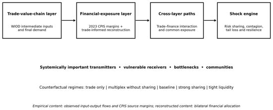
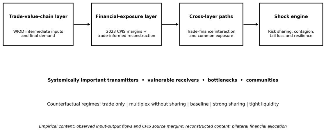
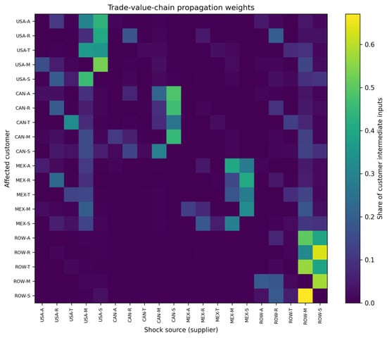
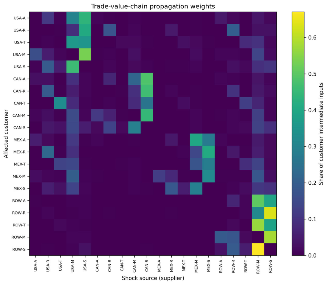
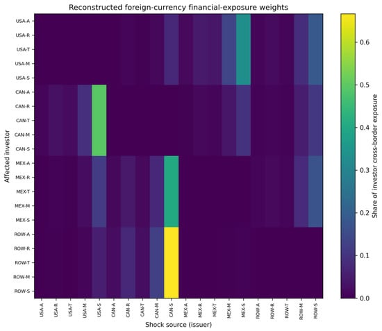
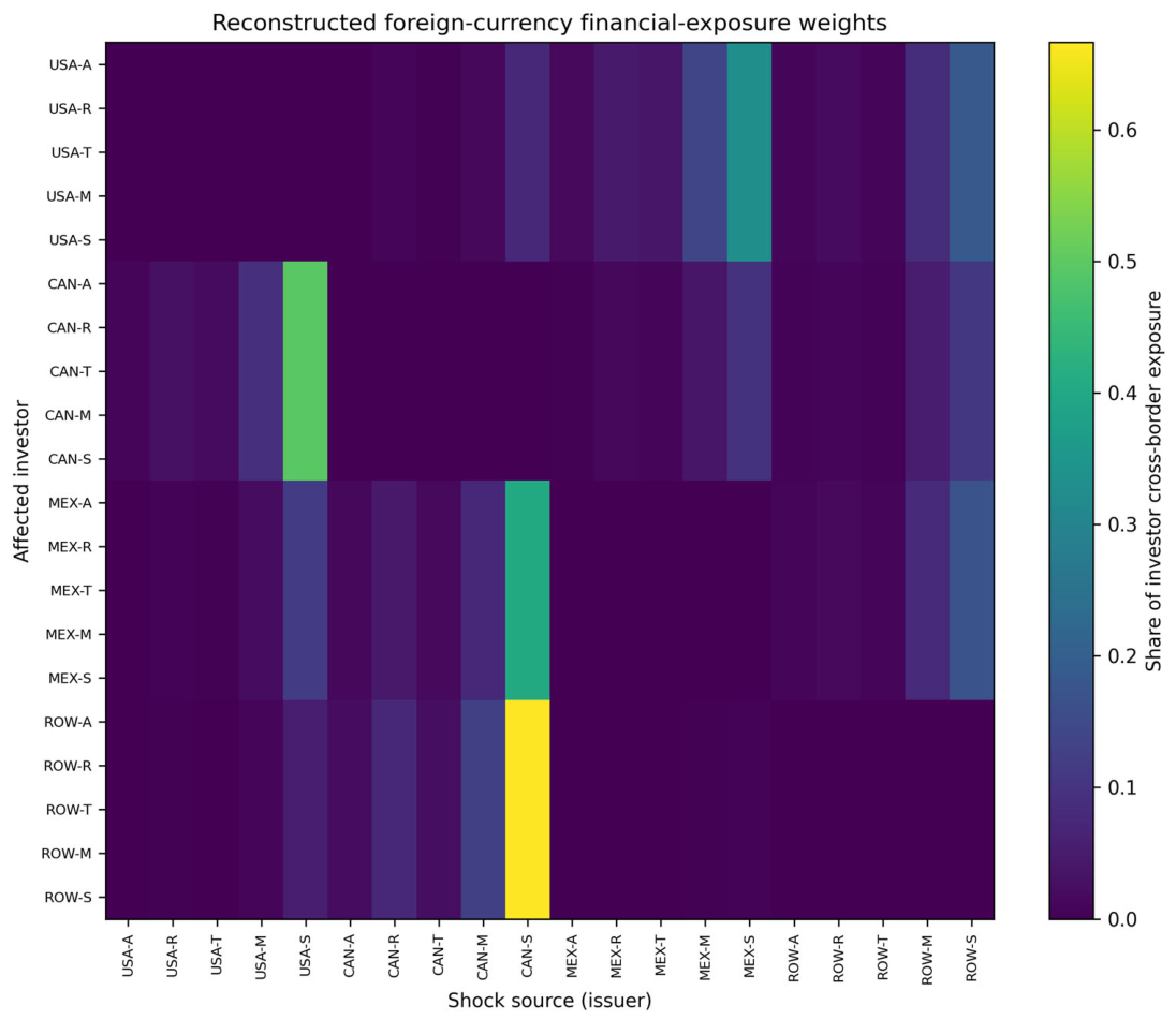
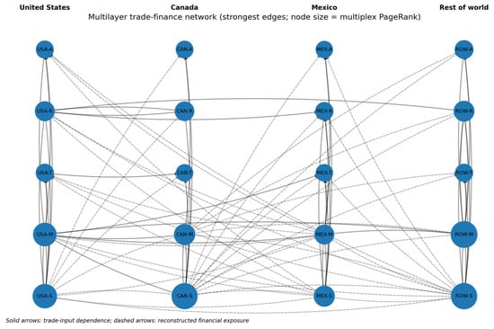
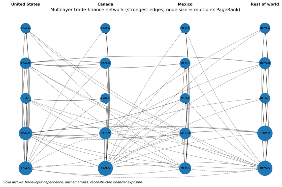
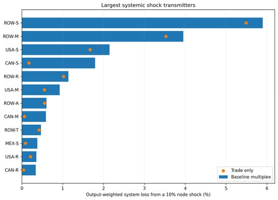
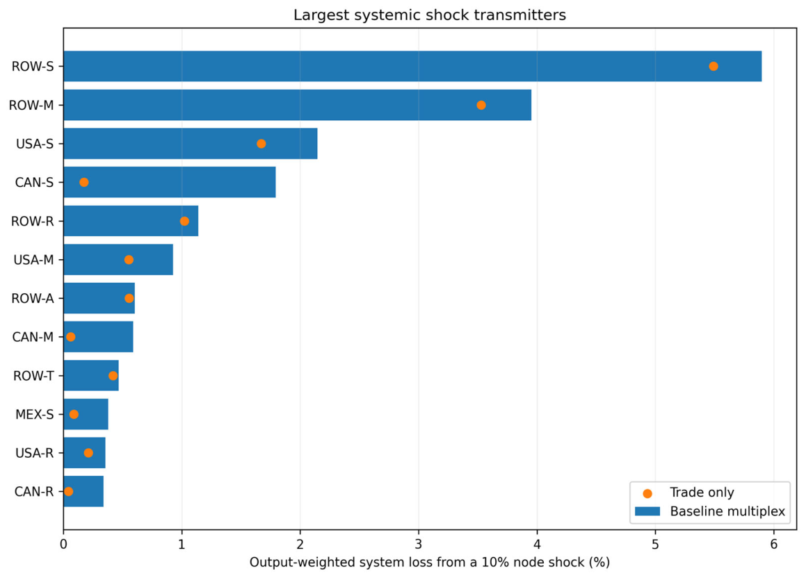
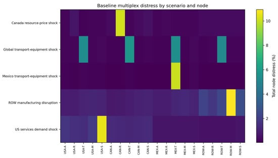
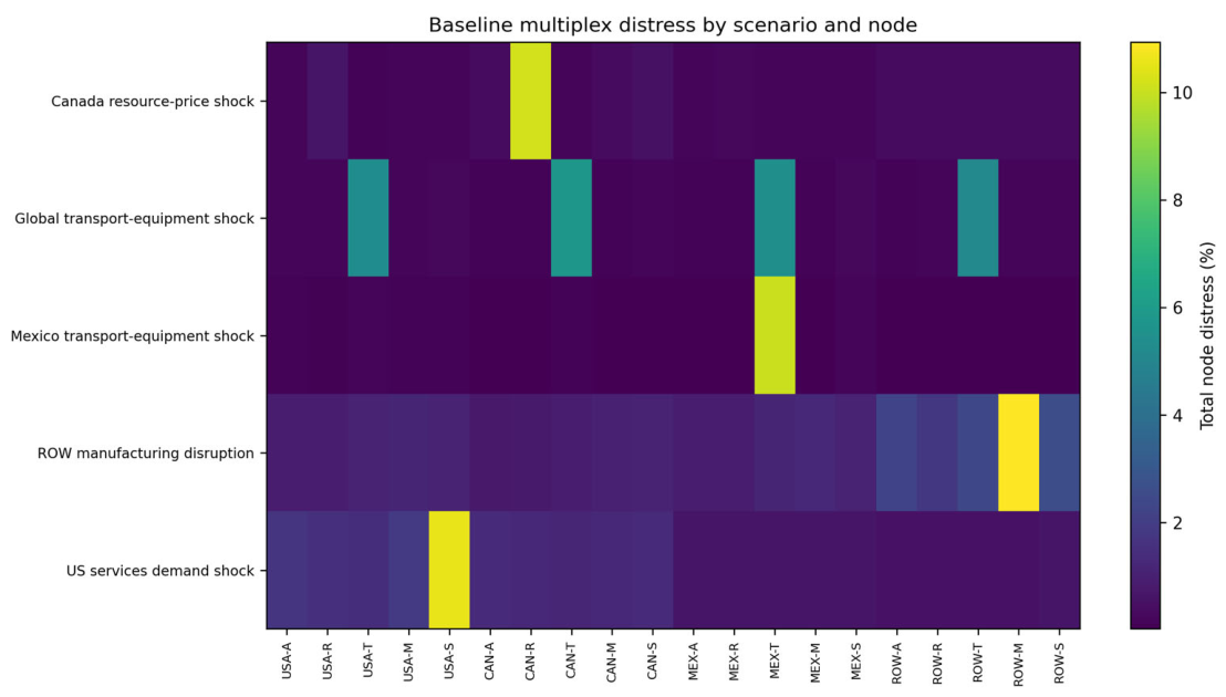
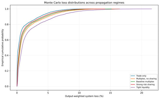
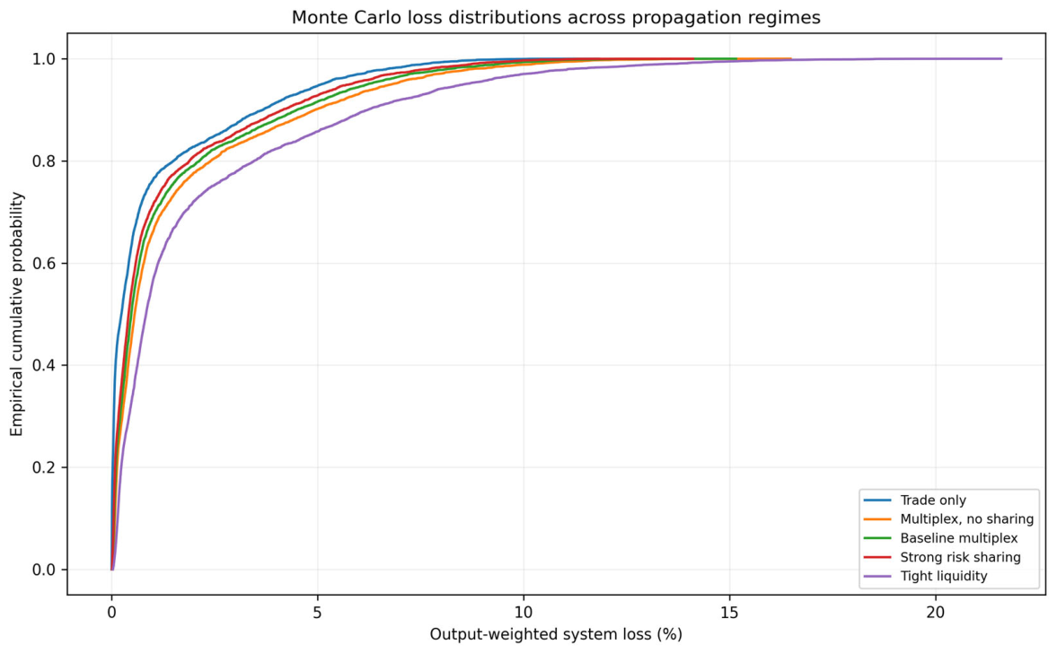
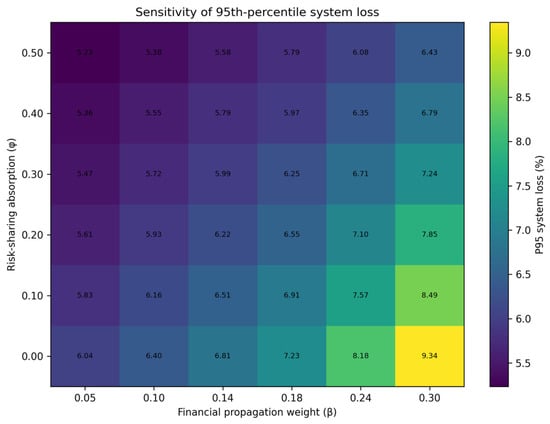
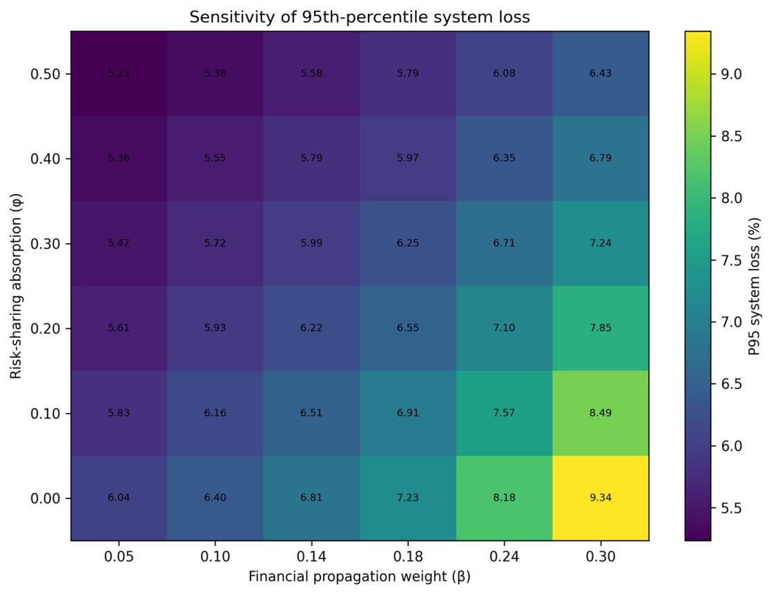

Disclaimer/Publisher’s Note: The statements, opinions and data contained in all publications are solely those of the individual author(s) and contributor(s) and not of MDPI and/or the editor(s). MDPI and/or the editor(s) disclaim responsibility for any injury to people or property resulting from any ideas, methods, instructions or products referred to in the content. |
© 2026 by the author. Licensee MDPI, Basel, Switzerland. This article is an open access article distributed under the terms and conditions of the Creative Commons Attribution (CC BY) license.