Calibration Method and Uncertainty Evaluation for X-Ray Fluorescence Chlorine Analyzers

Abstract

X-ray fluorescence (XRF) chlorine analyzers are widely used for chlorine determination in crude oil and petroleum products. Although analytical test procedures are standardized, a calibration-oriented uncertainty framework for the analyzer itself remains insufficiently developed. This study establishes a metrological framework for relative indication error and limit of detection (LOD), supported by repeatability and linearity evaluations, and compares uncertainty propagation using the Guide to the Expression of Uncertainty in Measurement (GUM) and the Monte Carlo method (MCM). For relative indication error, residual matrix mismatch was quantified using paired isooctane-based light-oil and 75 cSt mineral-oil reference materials and incorporated with measurement repeatability and certified-value uncertainty. At 100, 300 and 500 mg/L, GUM and MCM produced closely agreeing standard uncertainties of approximately 0.0115, 0.0103 and 0.0081, respectively. For LOD, both methods used the same dual-axis error-weighted regression, accounting for uncertainties in certified concentrations and mean instrumental responses; in the MCM, the regression was repeated for every simulated calibration data set. The resulting standard uncertainties were 0.0048 mg/L (GUM) and 0.0047 mg/L (MCM), and the MCM equal-tailed 95% coverage interval was 0.0122–0.0307 mg/L. The framework’s distinctive value is the consistent treatment of calibration measurands, matrix transfer and dual-axis error-weighted regression across both propagation methods. It provides an auditable GUM budget for routine calibration and certificate reporting, while MCM offers a verification route when repeated regression, finite-sample blank dispersion or asymmetric output intervals are important.

1. Introduction

Chlorine is a key corrosive element in crude oil and petroleum products; even trace amounts of chlorides can lead to catalyst poisoning in catalytic reforming units [1] and hydrochloric acid corrosion in distillation columns [2]. Consequently, standardized analytical methods, such as ASTM D4929 [3], have been established for the determination of organic chloride in crude oil and petroleum products, and accurate chlorine determination is important for process safety and product quality.

X-ray fluorescence (XRF) spectroscopy is widely used for quantitative chlorine analysis in petroleum products because sample preparation is simple, analysis is rapid and measurements are non-destructive [4]. Both monochromatic wavelength-dispersive X-ray fluorescence (MWDXRF) and energy-dispersive X-ray fluorescence (EDXRF) systems have advanced substantially [5]. In particular, double-curved-crystal MWDXRF instruments reduce spectral background and sulfur interference and can achieve chlorine detection limits as low as 0.13 mg/kg [6]. EDXRF remains important for rapid industrial screening.

Previous studies have developed bottom-up uncertainty budgets for particular XRF measurements [7] and compared GUM and MCM in ICP-OES, HPLC, GFAAS and LC-MS/MS applications [8,9,10,11]. These studies demonstrate the value of both propagation approaches, while JCGM 100 and JCGM 101 provide their general metrological basis [12,13]. However, the published work is mainly organized around sample-specific analytical results or established analytical models; it does not directly provide a calibration procedure for an XRF chlorine analyzer that links relative indication error, residual petroleum-matrix transfer and LOD to traceable uncertainty budgets.

Accordingly, this study contributes a calibration-oriented framework with three distinctive features: (1) the analyzer, rather than a single petroleum sample, is treated as the calibration object; (2) residual light-oil/heavy-oil mismatch after the built-in correction is quantified experimentally and propagated as an indication-error component with an explicit applicability boundary; and (3) the same dual-axis error-weighted regression model is used in both GUM and MCM for LOD, with the regression repeated in each Monte Carlo trial. Practically, the GUM budget provides an auditable route for routine calibration and certificate reporting, whereas MCM checks the effects of repeated regression, finite-sample blank dispersion and output asymmetry.

2. Measurement Principles and Calibration Methods

2.1. Measurement Response of the XRF Chlorine Analyzer

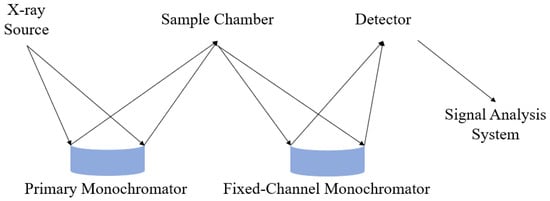
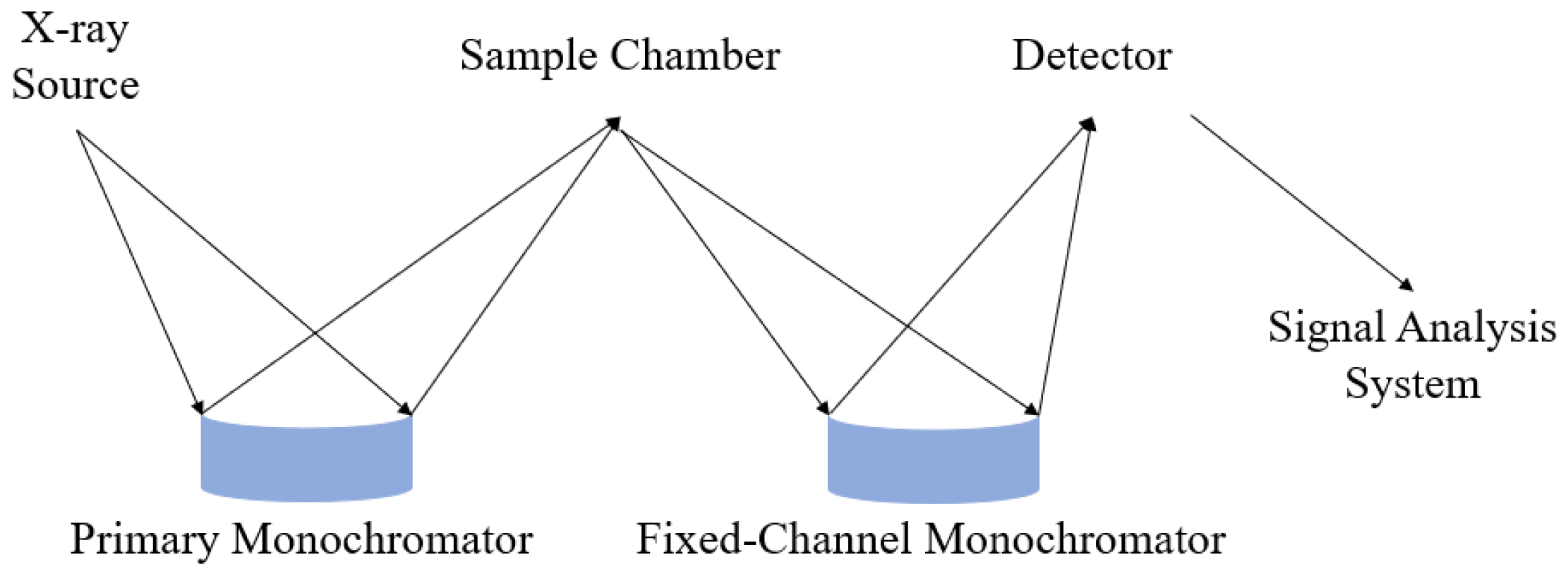
In an X-ray fluorescence chlorine analyzer, the chlorine-related response is obtained from the Cl Kα characteristic line generated under specified excitation and detection conditions. Element-specific X-ray emission and spectral-line energy provide the physical basis for selective chlorine detection [14]. The instrument converts the measured response into an indicated chlorine concentration through a calibration curve established using reference materials. A representative measurement configuration is shown in Figure 1.

Figure 1. Schematic measurement configuration of the XRF chlorine analyzer.

In XRF, attenuation and enhancement of characteristic radiation, background scattering, spectral interference and sample heterogeneity can change the response-to-concentration relationship. Studies of chlorine in crude oil and edible oils emphasize homogenization and matrix-appropriate calibration [15,16], while simultaneous chlorine/sulfur XRF and uncertainty studies identify matrix composition and calibration as material contributors [17]. Consequently, an analyzer calibrated with light-oil reference materials cannot be assumed to give an identical response for a heavier oil matrix without experimental verification.

Accordingly, this study treats the XRF chlorine analyzer as the object of calibration. The reported uncertainty applies to the instrument indication and LOD under the stated measurement and matrix conditions. Contributions from crude-oil distillation, extraction, recovery, or other sample-preparation steps are outside the present measurands and must be evaluated separately when an analytical method such as ASTM D4929 is implemented.

2.2. Experimental Measurement Conditions and Reference Materials

An E-lite500 X-ray fluorescence spectrometer (SuZhou JiaPu Scientific Co., Ltd., Suzhou, China) was used. The analyzer employs a doubly curved crystal and a silicon drift detector for low-background measurement of light elements in petroleum products. All measurement experiments used the conditions summarized in Table 1.

Table 1. Experimental measurement conditions.

Item	Parameter value
Analytical line	Cl Kα characteristic peak
X-ray tube voltage	30 kV
X-ray tube current	0.7 mA
Single measurement time	300 s

Certified reference materials (CRMs) for chlorine in light petroleum products were obtained from Sinopec Research Institute of Petroleum Processing Co., Ltd., Beijing, China. Their certified values and expanded uncertainties (k = 2) were taken directly from the certificates. Standard uncertainties were obtained by dividing the expanded uncertainties by the stated coverage factor, consistent with ISO/IEC Guide 98-3:2008 [18].

GBW(E)062534–GBW(E)062538 (1–30 mg/L) were used for the low-concentration calibration and LOD evaluation; GBW(E)062540–GBW(E)062542 (100, 300, and 500 mg/L) were used for indication-error evaluation. Table 2 summarizes their intended uses.

Table 2. Reference materials and their intended uses.

Reference Material No.	Certified Value	Expanded Uncertainty	Intended Use
GBW(E)062534	1.0 mg/L	0.15 mg/L	Low-concentration calibration curve fitting and limit of detection evaluation
GBW(E)062535	3.0 mg/L	0.11 mg/L
GBW(E)062536	5.0 mg/L	0.15 mg/L
GBW(E)062537	10.0 mg/L	0.25 mg/L
GBW(E)062538	30.0 mg/L	0.70 mg/L
GBW(E)062540	100 mg/L	1.50 mg/L	Relative indication error and uncertainty evaluation
GBW(E)062541	300 mg/L	5.00 mg/L
GBW(E)062542	500 mg/L	7.00 mg/L

The reference materials and blank matrix were introduced into the same type of sample cup and measured under identical instrumental conditions without dilution, so as to maintain consistency in sample loading and matrix conditions.

Residual matrix mismatch was examined with paired CRM sets at 100, 300, and 500 mg/L. The calibration was established with isooctane-based light-oil CRMs, after which both the light-oil CRMs and 75 cSt mineral-oil CRMs were measured three times at each matched nominal level under identical instrument conditions. The comparison therefore estimates the residual response difference after the analyzer’s built-in matrix correction; it is not a universal matrix-correction function.

All CRMs used in this comparison contained less than 3.0 g/kg sulfur. Sulfur was therefore not varied independently, and its possible spectral contribution was included only as part of the observed overall matrix mismatch. The resulting component is applicable to the tested isooctane/75 cSt mineral-oil pair and the stated low-sulfur conditions. Other crude oils, high-sulfur samples, or substantially different viscosities and compositions require matrix-matched CRMs or additional validation.

2.3. Calibration Design

The calibration design complements analytical standards such as ASTM D4929-24 [3]: the standard specifies sample treatment and chlorine determination, whereas the present design evaluates the analyzer’s metrological performance under controlled calibration conditions.

This study evaluated relative indication error, repeatability, linearity, and LOD; the uncertainty evaluation focused on relative indication error and LOD. The data-acquisition schemes are summarized in Table 3.

Table 3. Calibration items and data acquisition schemes.

Calibration Item	Reference Material or Sample	Data Acquisition Method	Output Quantity
Relative indication error	GBW(E)062540, GBW(E)062541, GBW(E)062542	Each concentration level was measured three times, and the arithmetic mean was taken as the instrument indication	Relative indication error
Measurement repeatability	GBW(E)062540, GBW(E)062541, GBW(E)062542	Ten consecutive measurements at each of 100, 300, and 500 mg/L	Standard deviation or relative standard deviation
Linearity	GBW(E)062534–GBW(E)062538	Each concentration level was measured three times, and the linear relationship was evaluated from the calibration data.	Slope, intercept, and correlation coefficient
Limit of detection	Isooctane blank matrix solution	The blank sample was measured 11 times, and the limit of detection was calculated in combination with the slope of the calibration curve	Limit of detection

• Relative indication error

Indication error characterizes the agreement between the instrument indication and the certified value. For concentrations within (0, 7] mg/L, it is expressed as an absolute indication error; for concentrations greater than 7 mg/L, it is expressed as a relative indication error. The present study evaluates relative indication error at 100, 300, and 500 mg/L.

• Limit of detection

According to the matrix of the reference materials, isooctane or another matrix-matched solution was selected as the blank sample. The blank was measured 11 times, and the experimental standard deviation was combined with the slope of the low-concentration calibration curve to determine the instrumental LOD [19].

3. Uncertainty Evaluation Using the GUM Framework

This section evaluates relative indication error and LOD in accordance with JCGM 100. The measurement models, input assumptions, uncertainty budgets and final results are retained; routine numerical substitutions are not repeated. The GUM evaluation included four main steps: defining the measurement model; assigning estimates, standard uncertainties, and relevant covariances to the input quantities; propagating these quantities using the first-order law of propagation of uncertainty; and reporting the combined and, where appropriate, expanded uncertainty. The GUM framework does not require all input quantities to follow normal distributions, but it does require an adequate measurement model and valid linearization. In this study, the input quantities for the indication-error model and the two LOD inputs were treated as mutually uncorrelated, while the covariance structure arising from the dual-axis error-weighted regression was retained in the estimation of the slope uncertainty.

3.1. Evaluation of Relative Indication Error Using the GUM Framework

3.1.1. Measurement Models and Measurement Methods

Measurement model: The dimensionless relative indication error was evaluated using Equation (1).

$$\Delta c_{\mathrm{r}}={\displaystyle \frac{\overline{c}-c_{\mathrm{s}}+{\delta }_{\mathrm{mat}}}{c_{\mathrm{s}}}},$$

(1)

where: $\Delta c_{\mathrm{r}}$ is the relative indication error of the instrument, dimensionless; $\overline{c}$ is the arithmetic mean of three replicate measurements, in mg/L; $c_{\mathrm{s}}$ is the concentration of the reference material, in mg/L; ${\delta }_{\mathrm{mat}}$ is the residual matrix-effect correction term.

Under the calibration conditions used in this study, no explicit residual matrix correction was applied; therefore, its estimated value was taken as zero. However, the matrix difference between light oil and heavy oil may introduce a residual bias, and the corresponding standard uncertainty was estimated from the supplementary matrix comparison experiment and included in the uncertainty budget.

Measurement method: Chlorine CRMs at 100, 300, and 500 mg/L were each measured three times under the conditions specified in Table 1, and the arithmetic mean was taken as the instrument indication. The relative indication error was then calculated according to the measurement model.

3.1.2. Uncertainty Analysis and Evaluation

Analysis of the measurement model shows that the uncertainty of the relative indication error arises mainly from $\overline{c}$, $c_{\mathrm{s}}$, and ${\delta }_{\mathrm{mat}}$. As the various input quantities are independent of one another, the formula for calculating the uncertainty of the relative indication error calibration results can be derived from the model equations as follows:

$$u_c=\sqrt{c_1^2{u}^2(\overline{c})+c_2^2{u}^2(c_{\mathrm{s}})+c_3^2{u}^2({\delta }_{\mathrm{mat}})},$$

(2)

The sensitivity coefficients are: $c_1={\displaystyle \frac{\partial \Delta c_r}{\partial \overline{c}}}={\displaystyle \frac{1}{c_{\mathrm{s}}}}$; $c_2={\displaystyle \frac{\partial \Delta c_r}{\partial c_{\mathrm{s}}}}=-{\displaystyle \frac{\overline{c}+{\delta }_{\mathrm{mat}}}{c_{\mathrm{s}}^2}}$; $c_3={\displaystyle \frac{\partial \Delta c_r}{\partial {\delta }_{\mathrm{mat}}}}={\displaystyle \frac{1}{c_{\mathrm{s}}}}$.

• Uncertainty components arising from instrument measurements $u(\overline{c})$

The standard uncertainty associated with the instrument measurement was evaluated from measurement repeatability and concentration readout resolution. The latter denotes the smallest increment of the displayed chlorine concentration. These two contributions are related: with finer resolution, variations due to repeatability are more readily observed, whereas with coarse resolution, the contribution from repeatability may become negligible. Therefore, to avoid double counting, only the larger of the two uncertainty contributions was included in the uncertainty budget.

• Uncertainty introduced by measurement repeatability $u_1(\overline{c})$:

The repeatability results and corresponding statistical quantities are listed in Table 4. The ten-result series was used to estimate the repeatability standard deviation; because the reported indication-error result is the mean of three consecutive measurements, its repeatability-related standard uncertainty was obtained by dividing the repeatability standard deviation by $\sqrt{3}$.

Table 4. Repeatability data and type A standard uncertainty evaluation.

Measurement No.	Calibration Points (mg/L)
	100 mg/L	300 mg/L	500 mg/L
1	98.17	314.56	509.63
2	97.98	315.61	510.11
3	97.86	314.89	510.36
4	98.24	315.24	509.22
5	98.11	315.71	509.94
6	97.64	315.02	511.01
7	97.55	314.99	510.87
8	97.68	314.87	511.12
9	98.36	314.25	511.34
10	98.71	313.98	511.26
$\overline{c}$ (mg/L)	98.030	314.912	510.486
$s$ (mg/L)	0.362	0.546	0.741
$u_1(\overline{c})$ (mg/L)	0.209	0.315	0.428

2.

Uncertainty introduced by concentration readout resolution $u_2(\overline{c})$:

The concentration readout resolution is 0.01 mg/L. Assuming a rectangular distribution over ±0.005 mg/L gives a standard uncertainty of 0.0029 mg/L.

In this study, the repeatability contribution was larger than the resolution contribution at all three concentration levels. Therefore, only the repeatability contribution was considered in the uncertainty budget.

• Uncertainty introduced by CRM certified values $u(c_{\mathrm{s}})$

The CRM certificates report expanded uncertainties of 1.50, 5.00 and 7.00 mg/L at 100, 300 and 500 mg/L, respectively, with k = 2. Division by the stated coverage factor gives standard uncertainties of 0.75, 2.50 and 3.50 mg/L.

• Uncertainty introduced by the residual matrix effect $u({\delta }_{\mathrm{mat}})$

XRF response is matrix dependent because attenuation/enhancement, spectral background and sample homogeneity can alter analytical sensitivity [3]. Petroleum studies likewise show that direct XRF measurement requires appropriate homogenization and matrix-matched calibration or correction. Therefore, repeatability and CRM certificate uncertainty alone do not cover transfer of a calibration from a light-oil matrix to a heavier oil matrix, and a residual matrix-mismatch term was included in the indication-error model.

The calibration was established with isooctane-based light-oil CRMs. Matched light-oil and 75 cSt mineral-oil CRMs were then measured three times at 100, 300 and 500 mg/L after the analyzer’s built-in matrix correction. All materials contained less than 3.0 g/kg sulfur; sulfur was not varied independently, so any remaining sulfur-related spectral contribution was included in the observed overall mismatch. At each level, the absolute difference between the two matrix means was used as the half-width of a zero-centered rectangular distribution, giving $u({\delta }_{\mathrm{mat}})={\Delta }_{\mathrm{mat}}/\sqrt{3}$. The resulting matrix differences and standard uncertainties are summarized in Table 5.

Table 5. Residual matrix-mismatch results after the built-in instrument correction.

Nominal Concentration (mg/L)	100	300	500
Mean measured value for the light-oil matrix (mg/L)	98.12	315.40	510.45
Mean measured value for the heavy-oil matrix (mg/L)	96.63	312.59	507.26
Light-oil/heavy-oil difference (mg/L)	−1.49	−2.81	−3.19
Standard uncertainty (mg/L)	0.86	1.62	1.84

Residual differences remained after correction and were retained in the uncertainty budget. This empirical component applies only to the tested analyzer and the low-sulfur isooctane/75 cSt mineral-oil matrices. Petroleum samples with substantially different composition, density, viscosity or sulfur content require matrix-matched CRMs or separate validation.

3.1.3. Summary and Combination of Uncertainty Components

The various uncertainty components are summarized in Table 6:

Table 6. Summary of uncertainty components for relative indication error.

Calibration Points	Sources of Uncertainty	Standard Uncertainty	Sensitivity Coefficient
100 mg/L	Measurement repeatability	0.209 mg/L	0.0100 L/mg
100 mg/L	CRM certified value	0.750 mg/L	−0.0098 L/mg
100 mg/L	Residual matrix effect	0.860 mg/L	0.0100 L/mg
300 mg/L	Measurement repeatability	0.315 mg/L	0.0033 L/mg
300 mg/L	CRM certified value	2.50 mg/L	−0.0035 L/mg
300 mg/L	Residual matrix effect	1.62 mg/L	0.0033 L/mg
500 mg/L	Measurement repeatability	0.428 mg/L	0.0020 L/mg
500 mg/L	CRM certified value	3.50 mg/L	−0.0020 L/mg
500 mg/L	Residual matrix effect	1.84 mg/L	0.0020 L/mg

At 100, 300, and 500 mg/L, the relative indication errors were −0.0197, 0.0497, and 0.0210, respectively. The corresponding GUM standard uncertainties were 0.0115, 0.0103, and 0.0081, and the expanded uncertainties (k = 2) were 0.0230, 0.0207, and 0.0162. All values are dimensionless.

Variance-component analysis clarifies the numerical results. At 100 mg/L, repeatability, CRM certification, and residual matrix mismatch contributed 3.3%, 40.8%, and 55.9% respectively. At 300 mg/L the corresponding contributions were 1.0%, 71.7%, and 27.3%; at 500 mg/L they were 1.1%, 78.2%, and 20.7%. Thus, matrix transfer dominated at the lowest level, whereas CRM certification dominated at the two higher levels.

3.2. Evaluation of Instrument LOD Using the GUM Framework

3.2.1. Measurement Model and Measurement Method

Measurement model: The LOD was evaluated using Equation (3), where $s_0$ is the experimental standard deviation of 11 blank responses (cps) and b is the low-concentration calibration slope (cps·L·mg⁻¹).

$$\mathrm{LOD}={\displaystyle \frac{3s_0}{b}},$$

(3)

Measurement method: An isooctane blank was measured 11 times to determine $s_0$. Five low-concentration CRMs, GBW(E)062534–GBW(E)062538, were each measured three times, and the mean response at each level was used for calibration. Because the certified concentrations and mean instrumental responses have non-negligible, heteroscedastic standard uncertainties, the slope was estimated by dual-axis error-weighted regression.

3.2.2. Uncertainty Analysis and Evaluation

According to Equation (3), the combined standard uncertainty of the LOD arises from the uncertainties associated with the calibration slope and the blank-response standard deviation. Assuming that the two input quantities are independent, the combined standard uncertainty is expressed as

$$u_c=\sqrt{c_1^2{u}^2(b)+c_2^2{u}^2(s_0)},$$

(4)

The sensitivity coefficients are: $c_1={\displaystyle \frac{\partial \mathrm{LOD}}{\partial b}}=-{\displaystyle \frac{3s_0}{b^2}}$; $c_2={\displaystyle \frac{\partial \mathrm{LOD}}{\partial s_0}}={\displaystyle \frac{3}{b}}$.

• Uncertainty introduced by the calibration slope b $u(b)$

The slope uncertainty was obtained from the covariance matrix of the dual-axis error-weighted fit. For the linear relation ${\overline{y}}_i=a+b{C}_i^{*}$, the intercept and slope were estimated by minimizing the objective function in Equation (5).

$${\chi }^2={\displaystyle \sum _{i=1}^N\left[\frac{{(c_{\mathrm{s},i}-C_i^{*})}^2}{u^2(c_{\mathrm{s},i})}+\frac{{({\overline{y}}_i-a-b{C}_i^{*})}^2}{u^2({\overline{y}}_i)}\right]},$$

(5)

where: N = 5; $c_{\mathrm{s},i}$ is the certified concentration at calibration point i; $C_i^{*}$ is the fitted latent concentration; ${\overline{y}}_i$ is the observed mean response; $u(c_{\mathrm{s},i})$ is obtained from the CRM certificate; and $u({\overline{y}}_i)$ is the Type A standard uncertainty of the mean response, evaluated from the three replicate responses.

The data and associated standard uncertainties used to establish the calibration curve are listed in Table 7.

Table 7. Calibration curve data and standard uncertainty.

Number	${\mathit{c}}_{\mathbf{s},\mathit{i}}$ (mg/L)	$\mathit{u}({\mathit{c}}_{\mathbf{s},\mathit{i}})$ (mg/L)	Measured (Response) Value (cps)			${\overline{\mathit{y}}}_{\mathit{i}}$ (cps)	$\mathit{s}({\mathit{y}}_{\mathit{i}})$ (cps)	$\mathit{u}({\overline{\mathit{y}}}_{\mathit{i}})$ (cps)
			1	2	3
1	1.0	0.075	126	122	121	123.0	2.956	1.708
2	3.0	0.055	344	347	348	346.3	2.367	1.367
3	5.0	0.075	577	581	576	578.0	2.959	1.708
4	10.0	0.125	1121	1124	1130	1125.0	5.325	3.075
5	30.0	0.350	3286	3295	3272	3284.3	13.609	7.857

The fitted relation was $\overline{y}=18.336+110.088C^{*}$, where b was 110.088 cps·L·mg⁻¹ and $u(b)$ was 1.13 cps·L·mg⁻¹.

• Uncertainty introduced by the blank-response standard deviation $s_0$ $u(s_0)$

The 11 blank responses were 32, 31, 32, 31, 31, 32, 32, 32, 30, 30, and 31 cps, giving a mean of 31.3 cps and $s_0$ of 0.786 cps.

For n = 11 normally distributed blank responses, the chi-square sampling model for the sample standard deviation gave $u(s_0)=0.18\mathrm{cps}$.

3.2.3. Summary and Combination of Uncertainty Components

The various uncertainty components are summarized in Table 8. The resulting LOD was 0.0214 mg/L, with a combined standard uncertainty of 0.0048 mg/L and an expanded uncertainty of 0.0096 mg/L (k = 2).

Table 8. Summary table of uncertainty components for instrument limit of detection.

Sources of Uncertainty	Standard Uncertainty	Sensitivity Coefficient
Slope b of the calibration line $u(b)$	1.13 cps·L·mg−1	−1.95 × 10−4 mg2·cps−1·L−2
Blank-response standard deviation $s_0$ $u(s_0)$	0.18 cps	0.0273 mg·cps−1·L−1

The blank-response dispersion dominated the LOD uncertainty; the contribution from the calibration slope was comparatively small under the present conditions.

4. Uncertainty Evaluation Using the Monte Carlo Method

4.1. Basic Principles and Implementation Steps of MCM

The MCM implementation followed JCGM 101 and propagated the same measurement functions and input information used in the corresponding GUM evaluations. Input probability distributions were assigned from repeatability or range-based Type A evaluations, CRM certificates and the matrix comparison. Inputs were sampled independently where no covariance information was available; dependence between fitted calibration parameters was generated by refitting the regression in every trial. Output distributions were summarized directly by their estimates, standard uncertainties and 95% coverage intervals. For the tabulated MCM results, the effective k value was calculated as the half-width of the equal-tailed 95% interval divided by the MCM standard uncertainty; it is reported as a descriptive ratio rather than as a GUM coverage factor.

4.2. Evaluation of Relative Indication Error Using the MCM Framework

Equation (1) was evaluated independently at 100, 300, and 500 mg/L. The main input quantities were the instrument measurement mean $\overline{c}$, the certified concentration $c_{\mathrm{s}}$, and the residual matrix-effect correction term ${\delta }_{\mathrm{mat}}$. The input quantities were assumed to be mutually independent.

For $\overline{c}$, a normal distribution was assigned. Its expectation was taken as the arithmetic mean of three replicate measurements, and its standard deviation was set equal to the corresponding standard uncertainty derived from the repeatability experiment.

For the certified concentration, a normal distribution was assigned, with the certified value given in the CRM certificate as the expectation and the standard uncertainty converted from the reported expanded uncertainty as the standard deviation. The distribution parameters at the three concentration levels are listed in Table 9.

Table 9. MCM input parameters for relative indication error.

Calibration Point (mg/L)	Input Value	Distribution Type	Mean (mg/L)	Standard Deviation (mg/L)
100	$\overline{c}$	Normal distribution	98.03	0.209
	$c_{\mathrm{s}}$	Normal distribution	100	0.750
	${\delta }_{\mathrm{mat}}$	Rectangular distribution	0	0.860
300	$\overline{c}$	Normal distribution	314.91	0.315
	$c_{\mathrm{s}}$	Normal distribution	300	2.500
	${\delta }_{\mathrm{mat}}$	Rectangular distribution	0	1.620
500	$\overline{c}$	Normal distribution	510.49	0.428
	$c_{\mathrm{s}}$	Normal distribution	500	3.500
	${\delta }_{\mathrm{mat}}$	Rectangular distribution	0	1.840

The residual matrix-effect correction term ${\delta }_{\mathrm{mat}}$ was assigned a zero-centered rectangular distribution because no explicit residual correction was applied to the measured result. The absolute difference observed between the light-oil and heavy-oil measurements at each concentration level was taken as the half-width of this distribution.

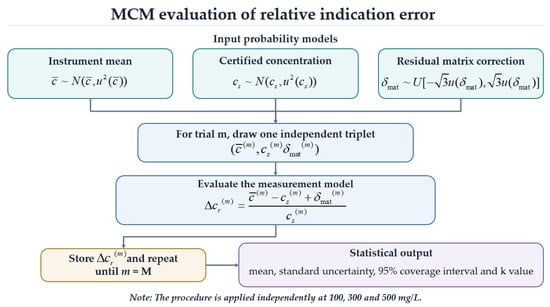
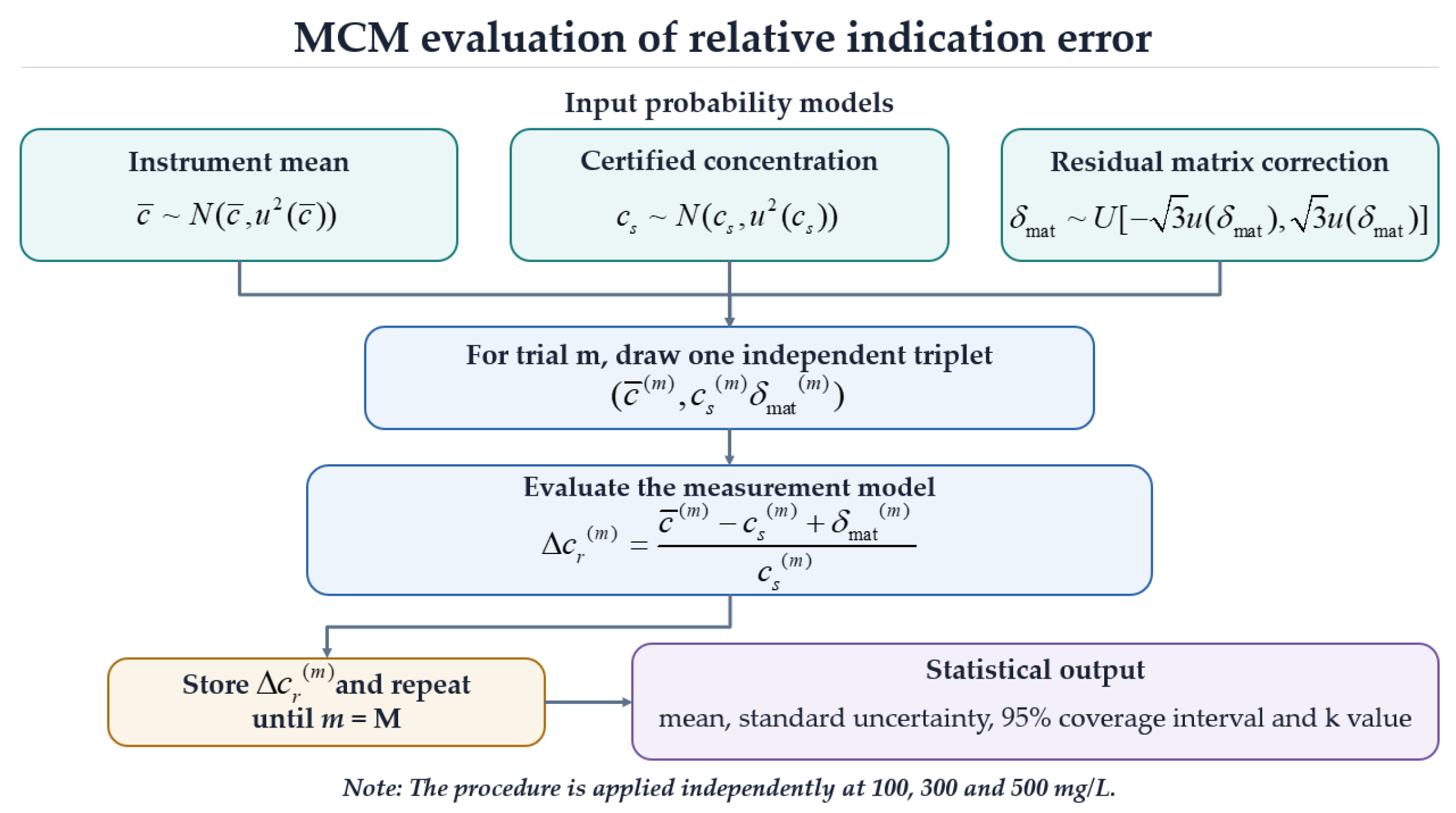
The sampling and model-evaluation procedure for the relative indication error is illustrated in Figure 2. The MATLAB implementation of the MCM evaluation for relative indication error is provided in Supplementary File S1.

Figure 2. MCM flowchart for the relative indication error evaluation.

In each trial, $\overline{c}$, $c_{\mathrm{s}}$ and ${\delta }_{\mathrm{mat}}$ were sampled and substituted into Equation (1). After 10⁶ trials, the mean and standard deviation of the output sample were taken as the estimate and standard uncertainty, respectively, and the 2.5th and 97.5th percentiles defined the equal-tailed 95% coverage interval.

Table 10 summarizes the MCM results. Their agreement with the GUM values supports the adequacy of first-order propagation for this indication-error model under the stated calibration conditions.

Table 10. MCM results for relative indication error.

Calibration Point (mg/L)	Estimate	Standard Uncertainty	95% Coverage Interval	k Value
100	−0.0196	0.0115	(−0.0414, 0.0024)	1.91
300	0.0498	0.0103	(0.0298, 0.0701)	1.95
500	0.0210	0.0081	(0.0053, 0.0370)	1.96

4.3. Evaluation of Instrument LOD Using the MCM Framework

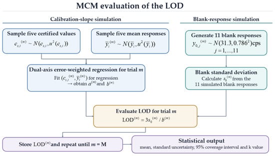
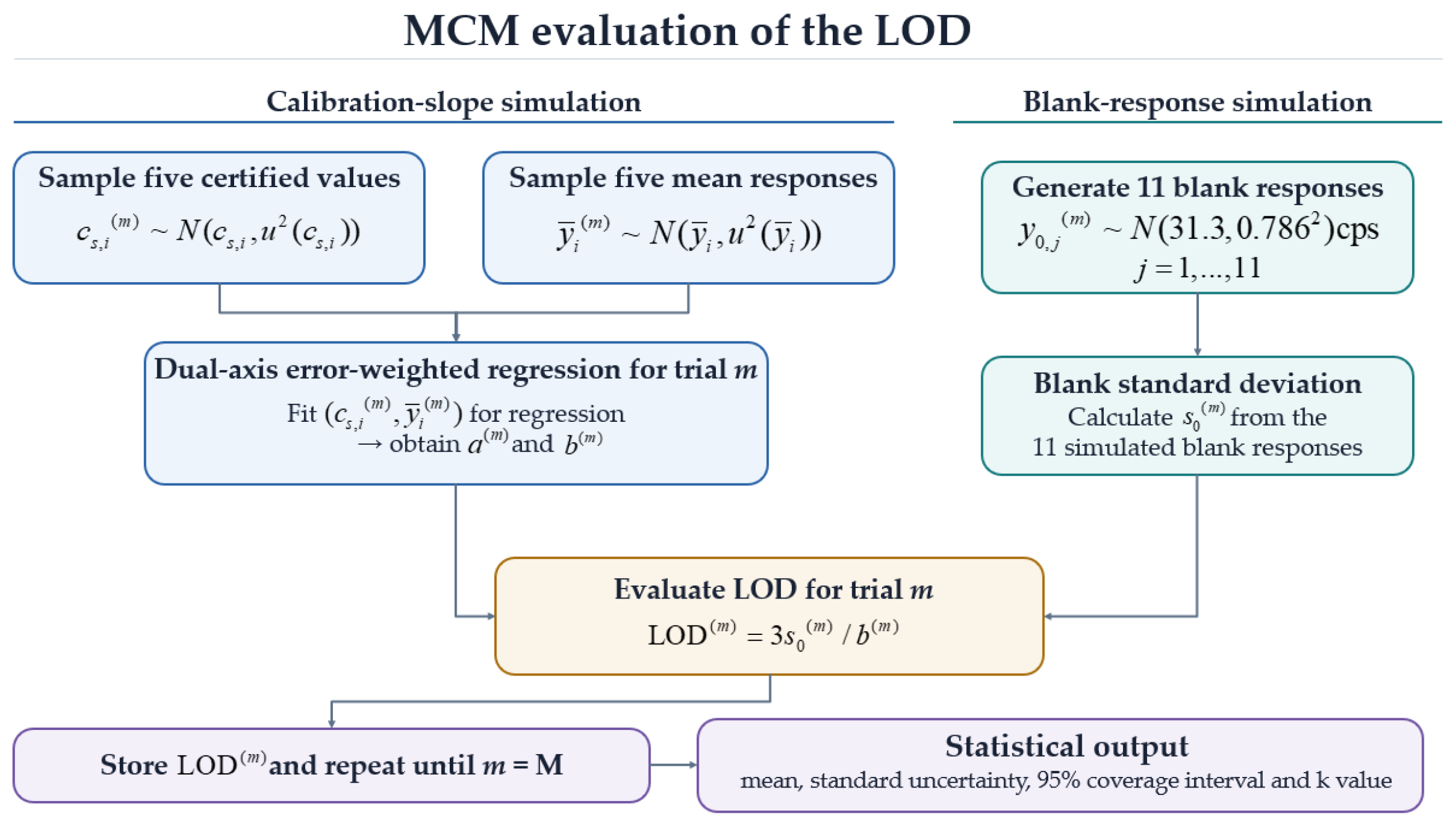
The LOD simulation comprised two synchronized branches (Figure 3). In the calibration branch, the five certified concentrations $c_{\mathrm{s},i}$ and five mean responses ${\overline{y}}_i$ were sampled from their assigned distributions. Each simulated five-point data set was then fitted by the same dual-axis error-weighted regression used in Section 3.2, with pointwise $u(c_{\mathrm{s},i})$, $u({\overline{y}}_i)$ and zero within-point error correlation. Sampling propagates possible input values, whereas weighting defines how the slope is estimated from each simulated data set; the two operations therefore do not duplicate an uncertainty component.

Figure 3. MCM flowchart for LOD evaluation.

In the blank branch, 11 responses were generated from $N\left(31.3,{0.786}^2\right)\mathrm{cps}$ and their sample standard deviation s₀ was calculated for that trial. The branches were combined through ${\mathrm{LOD}}^{(m)}=3s_0^{(m)}/b^{(m)}$. Repeating the complete procedure 10⁶ times propagated the uncertainties of both calibration coordinates, the fitted slope and the finite-sample blank dispersion.

Table 11 summarizes the input models used in the MCM evaluation of the LOD. The certified concentrations $c_{\mathrm{s},i}$ and mean instrumental responses ${\overline{y}}_i$ were assigned normal distributions based on their respective estimates and standard uncertainties. For each calibration level, the standard uncertainty of the mean response was evaluated from the three replicate responses using the range method. The blank response was represented by a normal distribution with a mean of 31.3 cps and a standard deviation of 0.786 cps. In each Monte Carlo trial, 11 blank responses were generated and their sample standard deviation was used as $s_0$.

Table 11. Summary table of distribution parameters for MCM assessment inputs of LOD.

Input	Calibration Point (mg/L)	Distribution Type	Mean	Standard Deviation
Concentration of standard material $c_{s,i}$	1.0	Normal distribution	1.0 mg/L	0.075 mg/L
	3.0		3.0 mg/L	0.055 mg/L
	5.0		5.0 mg/L	0.075 mg/L
	10.0		10.0 mg/L	0.125 mg/L
	30.0		30.0 mg/L	0.350 mg/L
Mean responses ${\overline{y}}_i$	1.0		123.0 cps	1.708 cps
	3.0		346.3 cps	1.367 cps
	5.0		578.0 cps	1.708 cps
	10.0		1125.0 cps	3.075 cps
	30.0		3284.3 cps	7.857 cps
Blank matrix response $y_{0,j}$	iso-octane j = 1, …, 11		31.3 cps	0.786 cps
Calibration curve parameters $a,b$	/	Not preset, generated in each trial by regression

The calibration intercept $a$ and slope b were not sampled independently. Instead, the five concentration-response pairs were sampled in each trial and refitted using dual-axis error-weighted regression. The resulting b and $s_0$ were then substituted into the LOD model. This procedure was repeated 10⁶ times to obtain the LOD distribution, standard uncertainty, and 95% coverage interval.

The MATLAB implementation of the MCM evaluation for LOD, including repeated dual-axis error-weighted regression, is provided in Supplementary File S2. The MCM gave an LOD estimate of 0.0209 mg/L, a standard uncertainty of 0.0047 mg/L and an equal-tailed 95% coverage interval of (0.0122, 0.0307) mg/L (Table 12). The slight positive skewness arose mainly from the finite-sample distribution of the blank-response standard deviation and the ratio form 3s₀/b, rather than from the slope term alone.

Table 12. MCM results for the limit of detection.

Statistic	Value
Estimate (mg/L)	0.0209
Standard uncertainty (mg/L)	0.0047
95% coverage interval (mg/L)	(0.0122, 0.0307)
k value	1.95

4.4. Comparison of GUM and MCM Results

For relative indication error, the absolute differences between the GUM and MCM standard uncertainties did not exceed 0.0001 in dimensionless units (Table 13). The close interval overlap is consistent with a smooth model and limited output asymmetry under the present input distributions.

Table 13. Comparison of GUM and MCM results for relative indication error.

Point (mg/L)	Method	Relative Indication Error	Standard Uncertainty	Coverage-Interval Half-Width	95% Coverage Interval
100	GUM	−0.0197	0.0115	0.0230	(−0.0427, 0.0033)
	MCM	−0.0196	0.0115	0.0219	(−0.0414, 0.0024)
300	GUM	0.0497	0.0103	0.0207	(0.0290, 0.0704)
	MCM	0.0498	0.0103	0.0202	(0.0298, 0.0701)
500	GUM	0.0210	0.0081	0.0162	(0.0048, 0.0372)
	MCM	0.0210	0.0081	0.0159	(0.0053, 0.0370)

GUM coverage results are reported as estimate ± 2u, whereas MCM coverage results are direct 2.5th–97.5th percentile intervals. Relative indication errors and their uncertainties are dimensionless. The coverage-interval half-width is 2u for the GUM results and half the difference between the percentile limits for the MCM results.

For LOD, the estimates differed by 0.0005 mg/L and the standard uncertainties by 0.0001 mg/L. The GUM interval (0.0118, 0.0310) mg/L, based on k = 2, closely overlapped the MCM percentile interval (0.0122, 0.0307) mg/L (Table 14). This agreement supports the GUM linearization for this data set but does not imply universal equivalence of the two propagation methods.

Table 14. Comparison of the limit of detection between GUM and MCM.

Method	LOD (mg/L)	Standard Uncertainty (mg/L)	Coverage-Interval Half-Width (mg/L)	95% Coverage Interval (mg/L)
GUM	0.0214	0.0048	0.0096	(0.0118, 0.0310)
MCM	0.0209	0.0047	0.0092	(0.0122, 0.0307)

For routine calibration, GUM is generally preferable when the model can be adequately linearized, input estimates and covariances can be summarized by standard uncertainties, and a transparent component-by-component budget is required. MCM is preferable, or provides a useful validation, when the model is strongly nonlinear, bounded or non-normal inputs are important, regression-parameter dependence must be propagated, or the output interval is asymmetric. Here, GUM is efficient for routine indication-error evaluation, whereas MCM is especially informative for checking the ratio-based LOD model with repeated calibration fits and finite-sample blank dispersion.

5. Discussion

The close GUM/MCM agreement demonstrates internal consistency under the stated calibration conditions; it does not establish that the methods are interchangeable in all applications. The choice between the GUM and MCM approaches should be based on model nonlinearity, input distributions, covariance information, and interval asymmetry.

The results also show that the uncertainty evaluation of XRF chlorine analyzers should not be limited to repeatability and certified-value uncertainty. For petroleum products, the response-to-concentration relationship may be affected by matrix composition, background scattering and coexisting elements. The supplementary light-oil/heavy-oil comparison confirmed that a residual matrix difference remained after instrument correction. Therefore, introducing the residual matrix effect into the indication-error model improves the completeness of the uncertainty budget and makes the calibration result more representative of practical petroleum-matrix measurements.

The proposed framework should be understood as a calibration-oriented complement to existing analytical standards for chlorine determination in petroleum products, rather than as an alternative sample-testing procedure. Existing standards mainly specify how chlorine content is determined in samples, whereas this study focuses on how the XRF chlorine analyzer itself is calibrated and how the uncertainty of its calibration characteristics is evaluated. Under matrix-controlled conditions, the framework can support metrological traceability and calibration certificate reporting. For samples with high sulfur content or substantially different matrix compositions, further matrix correction, matrix-matched calibration or validation using additional reference materials is still required.

6. Conclusions

This study established a calibration-oriented uncertainty framework for relative indication error and LOD of an XRF chlorine analyzer, supported by repeatability and linearity evaluations. For relative indication error, residual light-oil/heavy-oil mismatch was incorporated into the measurement model and uncertainty budget. At 100, 300 and 500 mg/L, GUM and MCM standard uncertainties agreed at approximately 0.0115, 0.0103 and 0.0081, respectively. For LOD, both methods used the same dual-axis error-weighted regression; the standard uncertainties were 0.0048 mg/L (GUM) and 0.0047 mg/L (MCM), and the MCM equal-tailed 95% interval was 0.0122–0.0307 mg/L.

The main contribution is a traceability-oriented link between analyzer calibration, empirical matrix-transfer uncertainty and dual-axis error-weighted regression-based LOD evaluation. Its practical advantage is a tiered workflow: GUM provides routine, auditable uncertainty budgets, while MCM validates cases involving regression dependence, finite-sample blank dispersion, nonlinearity or asymmetric intervals. The empirical matrix component is applicable to the tested analyzer and the low-sulfur isooctane/75 cSt mineral-oil matrices; application to substantially different sample matrices would require additional validation.

References

- Vogt, E.T.C.; Weckhuysen, B.M. The refinery of the future. Nature 2024, 629, 295–306. [Google Scholar] [CrossRef] [Scilit] [PubMed]
- Alabdullah, M.A.; Rodriguez Gomez, A.; Vittenet, J.; Bendjeriou-Sedjerari, A.; Xu, W.; Abba, I.A.; Gascon, J. A viewpoint on the refinery of the future: Catalyst and process challenges. ACS Catal. 2020, 10, 8131–8140. [Google Scholar] [CrossRef] [Scilit]
- ASTM D4929-24; Standard Test Method for Determination of Organic Chloride Content in Crude Oil (Procedure C). ASTM International: West Conshohocken, PA, USA, 2024. [CrossRef] [Scilit]
- Lu, C.; Li, Q.; Li, W.; Wang, K.; Zhang, P.; Wu, M.; Liu, Z. X-ray fluorescence detection system for trace elements in oil based on graphite curved crystal technology. Appl. Opt. 2024, 63, 4590–4597. [Google Scholar] [CrossRef] [Scilit]
- Vanhoof, C.; Bacon, J.R.; Fittschen, U.E.A.; Vincze, L. Atomic spectrometry update: Review of advances in X-ray fluorescence spectrometry and its special applications. J. Anal. At. Spectrom. 2024, 39, 2150–2201. [Google Scholar] [CrossRef] [Scilit]
- Lu, C.; Huang, C.; Wang, X.; Li, Q.; Wu, M.; Wang, K.; Liu, Z. High-precision and high-resolution X-ray fluorescence analysis system for chlorine elements based on double-curved crystal technology. Appl. Spectrosc. 2025, 79, 1198–1205. [Google Scholar] [CrossRef] [Scilit] [PubMed]
- Devi, P.S.R.; Chavan, T.A.; Ghosh, M.; Swain, K.K. Total reflection X-ray fluorescence analysis of high-purity quartz: A bottom-up approach of uncertainty evaluation. Spectrochim. Acta Part B At. Spectrosc. 2021, 178, 106127. [Google Scholar] [CrossRef] [Scilit]
- Li, C.; Xu, L.; Wang, P.; Tang, D.; Xu, J.; Wang, H.; Wang, Y.; Wang, S.; Lu, W. Uncertainty evaluation of Cd concentration in sphalerite by ICP-OES: A comparative study between GUM and Monte Carlo methods. Anal. Methods 2025, 17, 9234–9243. [Google Scholar] [CrossRef] [Scilit] [PubMed]
- Haidara, H.; Assirey, E.A.; Saffaj, T.; Ihssane, B. Metrological Evaluation of Metopimazine HPLC Assay: ISO-GUM and Monte Carlo Simulation Approaches. Pharmaceutics 2025, 17, 1316. [Google Scholar] [CrossRef] [Scilit] [PubMed]
- Theodorou, D.; Meligotsidou, L.; Karavoltsos, S.; Burnetas, A.; Dassenakis, M.; Scoullos, M. Comparison of ISO-GUM and Monte Carlo methods for the evaluation of measurement uncertainty: Application to direct cadmium measurement in water by GFAAS. Talanta 2011, 83, 1568–1574. [Google Scholar] [CrossRef] [Scilit] [PubMed]
- Kim, S.Y.; Shin, D.W.; Hyun, J.; Kwon, N.H.; Cheong, J.C.; Paeng, K.-J.; Lee, J.; Kim, J.Y. Uncertainty Evaluation for the Quantification of Urinary Amphetamine and 4-Hydroxyamphetamine Using Liquid Chromatography–Tandem Mass Spectrometry: Comparison of the Guide to the Expression of Uncertainty in Measurement Approach and the Monte Carlo Method with R. Molecules 2023, 28, 6803. [Google Scholar] [CrossRef] [Scilit] [PubMed]
- JCGM 100:2008; Evaluation of Measurement Data—Guide to the Expression of Uncertainty in Measurement. Joint Committee for Guides in Metrology: Sèvres, France, 2008. [CrossRef] [Scilit]
- JCGM 101:2008; Evaluation of Measurement Data—Supplement 1 to the Guide to the Expression of Uncertainty in Measurement—Propagation of Distributions Using a Monte Carlo Method. Joint Committee for Guides in Metrology: Sèvres, France, 2008. [CrossRef] [Scilit]
- Zschornack, G. Handbook of X-Ray Data; Springer: Berlin/Heidelberg, Germany, 2007; pp. 7–10, 40–49. [Google Scholar]
- Doyle, A.; Saavedra, A.; Tristão, M.L.B.; Nele, M.; Aucélio, R.Q. Direct chlorine determination in crude oils by energy dispersive X-ray fluorescence spectrometry: An improved method based on a proper strategy for sample homogenization and calibration with inorganic standards. Spectrochim. Acta Part B At. Spectrosc. 2011, 66, 368–372. [Google Scholar] [CrossRef] [Scilit]
- Nicolas, M.; Theurillat, X.; Redeuil, K.; Nagy, K. Monochromatic wavelength dispersive X-ray fluorescence as a tool for monitoring the source of chlorine in the formation of monochloropropane-diol esters during vegetable oil refining. J. Agric. Food Res. 2022, 8, 100297. [Google Scholar] [CrossRef] [Scilit]
- Zhao, W.Z.; Lu, B.; Lv, S.N.; Zhou, C.F.; Yang, Y. Simultaneous determination of chlorine and sulfur in geochemical reference samples by wavelength dispersive X-ray fluorescence spectrometry. New J. Chem. 2020, 44, 11224–11230. [Google Scholar] [CrossRef] [Scilit]
- ISO/IEC Guide 98-3:2008; Uncertainty of Measurement—Part 3: Guide to the Expression of Uncertainty in Measurement (GUM:1995). International Organization for Standardization: Geneva, Switzerland, 2008.
- Yuan, L.J.; Jia, Y.H.; Cheng, D.W. Study on methods of detection limit in XRF spectrometry. Spectrosc. Spectr. Anal. 2023, 43, 412–418. [Google Scholar] [CrossRef]
Disclaimer/Publisher’s Note: The statements, opinions and data contained in all publications are solely those of the individual author(s) and contributor(s) and not of MDPI and/or the editor(s). MDPI and/or the editor(s) disclaim responsibility for any injury to people or property resulting from any ideas, methods, instructions or products referred to in the content. |
© 2026 by the authors. Licensee MDPI, Basel, Switzerland. This article is an open access article distributed under the terms and conditions of the Creative Commons Attribution (CC BY) license.