


Abstract
The nondestructive detection of sodium chloride in mural plaster layers is important for assessing salt-related deterioration in cultural heritage materials. However, the weak and indirect spectral response of sodium chloride makes accurate hyperspectral detection challenging. This study developed a hyperspectral regression framework centered on Sparrow Search Algorithm (SSA) optimization, in which continuous wavelet transform (CWT) was used to construct multiscale spectral representations and Pearson correlation analysis combined with the Successive Projections Algorithm (PCC-SPA) was used for compact variable selection. Partial least squares regression (PLSR), support vector regression (SVR), extreme gradient boosting (XGBoost), SSA-optimized SVR, and SSA-optimized XGBoost were evaluated under nested stratified specimen-grouped five-fold cross-validation. Feature selection and hyperparameter optimization were independently performed within each outer training fold, whereas the held-out specimens were reserved for performance evaluation. SVR-SSA maintained high predictive capability across both conventional and multiscale spectral representations. SG + SNV yielded an R2 of 0.8167 ± 0.0690 and an RMSE of 0.3701 ± 0.0636 percentage points. Scale 6 CWT achieved closely comparable R2 and RMSE values of 0.8100 ± 0.0812 and 0.3731 ± 0.0767 percentage points, respectively, together with a lower MAE of 0.2788 ± 0.0620 percentage points. Among the ten CWT scales, Scale 6 achieved the highest mean prediction accuracy, whereas Scale 2 provided the best comprehensive balance between predictive accuracy and fold-to-fold stability. These results demonstrate that the effectiveness of SSA optimization depends on the input feature representation and that CWT provides scale-resolved information beyond a single conventional spectral representation. The proposed framework provides methodological support for the nondestructive quantitative assessment of NaCl-related deterioration in mural plaster materials and establishes a basis for further application in mural conservation.
1. Introduction
Ancient murals are an important part of Chinese cultural heritage, preserving the artistic styles, religious beliefs, and social information of specific historical periods and possessing irreplaceable historical, artistic, and scientific value [1]. However, during long-term preservation, fluctuations in temperature and humidity, groundwater migration, and related processes can promote the transport and crystallization of soluble salts, thereby inducing mural deterioration such as efflorescence, hollowing, flaking, and detachment [2,3].
Conventional salt detection largely relies on field sampling followed by chemical analysis [4]. Although such methods can provide accurate quantitative results, they are inherently destructive and inefficient, making them unsuitable for the in situ, rapid, and large-area monitoring required for precious murals. By contrast, hyperspectral techniques integrate spectral and spatial information and enable non-contact detection, offering clear advantages for identifying subtle spectral differences. Previous studies have explored the use of hyperspectral methods for inverting salt content in mural plaster layer samples and have reported encouraging results. Nevertheless, challenges still remain, such as insufficient feature extraction, limited model stability, and weak generalization capability [5,6].
Hyperspectral inversion of salt content in murals mainly involves three key components which are spectral preprocessing, feature selection, and model establishment. Spectral preprocessing is essential for reducing measurement noise and improving the comparability of hyperspectral observations. Savitzky–Golay (SG) smoothing can suppress high-frequency random noise, whereas standard normal variate (SNV) transformation can reduce baseline and multiplicative scattering differences among specimens. These conventional procedures provide an effective single-representation description of the spectra but do not explicitly characterize spectral variations across different smoothing scales. Continuous wavelet transform (CWT), by contrast, decomposes spectral signals jointly in the wavelength and scale domains and can represent local spectral-shape variations at multiple levels of detail [7,8]. CWT should therefore be considered a complementary multiscale feature-construction strategy rather than simply a replacement for conventional preprocessing. Notably, the optimal wavelet scale varies with the target under investigation. Yao et al. [9] reported that sensitive wavelet features were mainly distributed at relatively high scales for wheat canopy leaf biomass estimation, whereas Cheng et al. [10] found that features at low scales provided better discrimination in rubber tree powdery mildew detection. Li et al. [11] further demonstrated a clear relationship between the hyperspectral response of soil organic matter and decomposition scale. Therefore, a complete scale-wise evaluation is required to determine how multiscale wavelet representations affect feature relevance, prediction accuracy, and model stability in hyperspectral NaCl estimation.
Spectral preprocessing and feature selection alone are insufficient to achieve accurate hyperspectral inversion of salt content in murals, because the relationship between salt content and spectral response is inherently complex, and the applicability of different models varies under small-sample and high-dimensional feature conditions. Partial least squares regression (PLSR) has clear advantages in handling high-dimensional collinear data, whereas support vector regression (SVR) is well suited for nonlinear modeling with limited samples. Previous studies have shown that both PLSR and SVR have been widely applied in quantitative hyperspectral inversion [12,13,14]. Using airborne hyperspectral data, Canero et al. [15] developed models for soil organic matter and clay content based on PLSR and SVR, and found that SVR outperformed PLSR for both soil properties, indicating that model suitability may differ across inversion targets. Wong et al. [16] used hyperspectral data combined with PLSR to predict physiological traits in legumes, further confirming the effectiveness of PLSR for modeling high-dimensional spectral data. As an ensemble learning algorithm, extreme gradient boosting (XGBoost) has strong nonlinear fitting capability and good generalization performance, and has recently been applied in quantitative hyperspectral inversion studies [17,18]. Wu et al. [19] developed an inversion model for copper content in maize leaves based on derivative reflectance spectroscopy (DRS) preprocessing and XGBoost. Good predictive performance was obtained, demonstrating the suitability of XGBoost for modeling high-dimensional nonlinear hyperspectral data. Further studies have shown that combining feature optimization with parameter tuning can further improve the performance of nonlinear models. Using hyperspectral data, Yu et al. [20] developed a particle swarm optimization support vector regression (PSO-SVR) model for high-accuracy prediction of water content, suggesting that swarm intelligence algorithms have considerable potential for SVR parameter optimization. Tan et al. [21] used an improved SSA to optimize the parameters of an SVR model for rapid hyperspectral prediction of soybean fat and protein contents. Gu et al. [22] further developed an XGBoost-SSA model for inversion of leaf nitrogen content in wheat, demonstrating that SSA optimization can improve the predictive accuracy and generalization capability of nonlinear models to a certain extent.
Previous studies have demonstrated the potential of SVR and XGBoost for quantitative hyperspectral analysis. However, the performance of these nonlinear models depends strongly on the selected hyperparameters, particularly under small-sample and high-dimensional conditions. Although SSA has been used to optimize nonlinear regression models in agricultural and environmental applications, its effectiveness for hyperspectral NaCl estimation in mural plaster materials has not been systematically evaluated. Moreover, the benefit of SSA optimization may vary with the spectral feature representation supplied to the model.
CWT provides a means of constructing scale-dependent spectral representations, but the relationships among CWT scale, feature relevance, predictive performance, model stability, and SSA optimization remain unclear for NaCl-containing mural plaster materials. Therefore, the principal objective of this study was to evaluate an SSA-optimized nonlinear regression framework across conventional and multiscale spectral representations. Specifically, this study: (1) used SSA to optimize the key hyperparameters of SVR and XGBoost; (2) compared SSA-optimized models with fixed-parameter SVR, XGBoost, and PLSR using four representative feature sets; (3) evaluated the complete set of ten CWT scales using the strongest regression-model family; and (4) jointly assessed mean predictive accuracy and fold-to-fold stability to clarify the scale dependence of CWT features and the feature dependence of SSA optimization. The study aimed to establish a rigorously evaluated hyperspectral framework for quantitative NaCl assessment in mural plaster layers and to clarify the complementary roles of multiscale CWT feature construction and SSA-based model optimization.
2. Materials and Methods
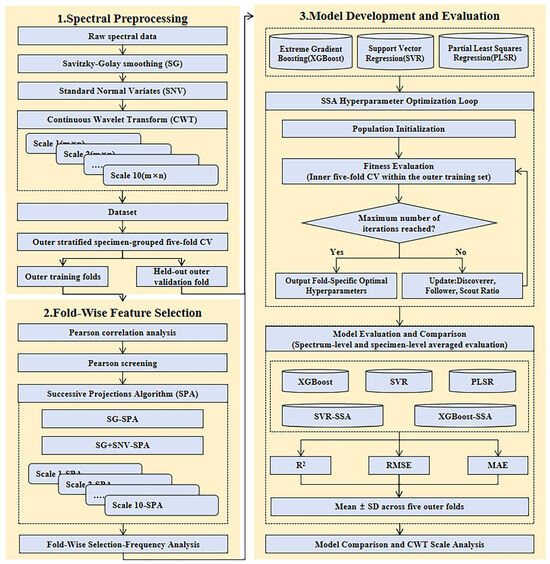
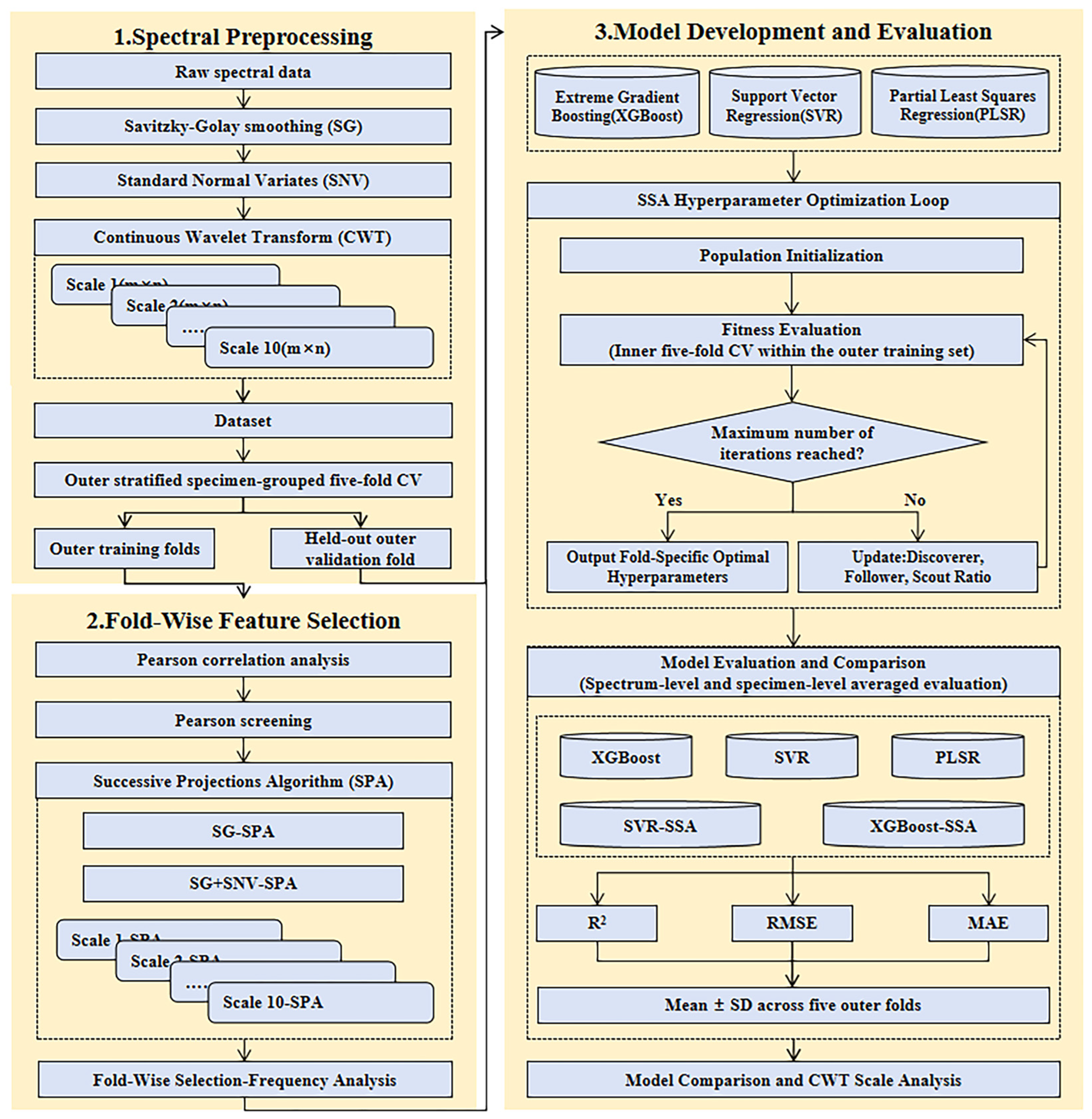
As shown in Figure 1, the analytical workflow consisted of three interconnected stages: spectral feature construction, nested model development, and model evaluation. First, the raw spectra were smoothed using the Savitzky–Golay method. Standard normal variate transformation was subsequently applied to reduce baseline and multiplicative scattering differences, and continuous wavelet transform was used to construct ten scale-dependent spectral representations. The resulting feature sets included SG, SG + SNV, and CWT Scales 1–10.
Figure 1.
Flowchart of the research methodology.
Second, model development was conducted under nested stratified specimen-grouped five-fold cross-validation. In each outer iteration, four folds were used for model development and the remaining fold was retained for independent out-of-fold prediction. Within each outer training fold, the repeated spectra of each physical specimen were averaged for supervised feature selection. Pearson correlation screening was first used to retain the 200 highest-ranked candidate variables, after which near-constant variables were removed, the remaining variables were standardized using training-derived parameters, and SPA was applied to identify a compact low-collinearity subset. The SPA subset size was determined by inner specimen-level five-fold cross-validation. Using the selected variables, PLSR, fixed-parameter SVR, and fixed-parameter XGBoost models were established. SSA was further used to optimize SVR and XGBoost hyperparameters, with the inner grouped five-fold RMSE used as the fitness function. After the maximum number of iterations was reached, the fold-specific optimal parameters were used to refit the corresponding model on the complete outer training fold and to predict the held-out specimen groups.
Third, model performance was evaluated using out-of-fold predictions at both the spectrum and physical-specimen levels. For specimen-level evaluation, the four predictions corresponding to the same physical specimen were averaged. R2, RMSE, and MAE were calculated separately for each outer fold and summarized as the mean ± standard deviation across the five folds. The model comparison was conducted in two stages. In Stage 1, PLSR, SVR, SVR-SSA, XGBoost, and XGBoost-SSA were compared using SG + SNV, Scale 2, Scale 6, and Scale 7. In Stage 2, the strongest model family was evaluated using SG + SNV and all ten CWT scales to quantify scale sensitivity and to identify the CWT representations associated with the highest mean accuracy and the best accuracy–stability balance.
2.1. Sample Preparation and Data Acquisition
In this study, mural plaster layer samples with different salt concentrations were prepared in the laboratory according to traditional ancient mural production methods [23,24]. The raw materials were desalted, naturally air-dried, and sieved to reduce interference from impurities. Each mural plaster layer sample consisted of a bottom coarse plaster and a surface fine plaster. The coarse plaster was prepared by mixing soil, sand, and wheat straw. After deionized water was added and the mixture was thoroughly stirred, it was filled into an iron mold with a diameter of 6 cm and a height of 2 cm. The fine plaster was prepared from soil, fine sand, and cotton fiber. Sodium chloride was dissolved in a fixed amount of distilled water according to the designed concentration, thoroughly mixed with the fine plaster materials, and then coated onto the surface of the coarse plaster.
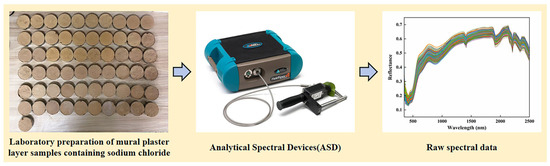
As shown in Figure 2, a total of 61 salt-containing mural plaster layer samples were prepared, with sodium chloride concentrations ranging from 0% to 3.00% at intervals of 0.05%. Salt content was expressed as the percentage of sodium chloride mass relative to the total mass of the solid mixture in the fine plaster. Sample weighing was carried out using an electronic balance (Shanghai Hochoice Apparatus Manufacturer Co., Ltd., Shanghai, China) with a precision of 0.001 g to ensure the accuracy and repeatability of the concentration settings. After preparation, all samples were left to dry under natural indoor conditions, and hyperspectral measurements were acquired after the moisture condition had stabilized.
Figure 2.
Mural plaster layer samples containing sodium chloride, spectral acquisition equipment, and raw spectral curves. The colored lines represent the 244 raw reflectance spectra obtained from the 61 mural plaster specimens.
The reflectance of the mural plaster layer samples was collected using a FieldSpec 4 spectroradiometer manufactured by Analytical Spectral Devices, Inc. (Boulder, CO, USA). The instrument covers a spectral range of 350–2500 nm, with a spectral resolution of 3 nm and a sampling interval of 1.4 nm in the 350–1000 nm range, and a spectral resolution of 8 nm and a sampling interval of 2 nm in the 1000–2500 nm range. Before measurement, the instrument was preheated for 20 min to ensure stable operating conditions of the light source and detector. During measurement, reflectance calibration was performed using the standard white reference panel supplied with the FieldSpec 4 spectroradiometer, and the probe was positioned vertically over the sample surface. For each mural plaster specimen, spectra were collected from four different positions to reduce the influence of local surface heterogeneity. The four positional spectra acquired in one measurement were averaged to obtain one representative spectrum for that measurement. This acquisition procedure was repeated four times for each specimen. Therefore, four averaged spectra were obtained from each specimen, resulting in a total of 244 spectral curves from 61 specimens. The four averaged spectra from the same specimen shared the same sodium chloride concentration and were treated as repeated spectral observations. In the data matrix, the spectra were arranged by measurement round; therefore, the four repeated averaged spectra from the same specimen were treated as one group during model validation.
2.2. Data Preprocessing
Continuous Wavelet Transform
CWT characterizes spectral variations from both the wavelength-position and smoothing-scale dimensions. It can attenuate high-frequency noise while preserving local spectral features, thereby enhancing subtle spectral information associated with sodium chloride content. By decomposing one-dimensional spectra into wavelet coefficients at different scales, CWT provides a richer basis for subsequent feature-band selection [25]. The mathematical expression of CWT is as follows:
where denotes spectral reflectance, is the wavelength, is the mother wavelet function, is the scale factor, is the translation factor, and is the wavelet coefficient corresponding to a given scale and wavelength position.
In this study, the Mexican Hat wavelet (mexh) was selected as the mother wavelet. As the second derivative form of a Gaussian function, mexh is sensitive to local peak-valley variations and absorption features, making it suitable for enhancing weak spectral features in hyperspectral data. The scale factor was set from 21 to 210, yielding a total of 10 decomposition scales. For each sample, wavelet coefficients were calculated separately at different scales, generating wavelet coefficient curves aligned with the original wavelengths. The wavelet coefficients of all samples at the same scale were then assembled column-wise to form the wavelet feature matrix for that scale.
2.3. Nested Specimen-Grouped Validation and Feature Selection
2.3.1. Dataset Partitioning
To ensure that repeated spectral observations from the same physical specimen did not appear simultaneously in the training and validation subsets, the outer cross-validation partitions were constructed at the physical-specimen level rather than at the individual spectrum level. The four repeated averaged spectra obtained from each specimen were always assigned to the same outer fold. Stratified specimen-grouped five-fold cross-validation was used, with grouping based on physical specimen and stratification based on NaCl concentration. The same outer-fold assignments were used for all feature sets and regression models.
In each outer iteration, four folds were used as the outer training set, and the remaining fold was retained as the outer validation set. All data-dependent procedures, including variable standardization, Pearson correlation screening, Successive Projections Algorithm (SPA) subset selection, PLSR latent-variable selection, and SSA hyperparameter optimization, were conducted exclusively using the corresponding outer training specimens. The held-out outer validation specimens were used only for prediction and performance calculation and did not participate in feature selection, preprocessing-parameter estimation, model tuning, or model fitting.
Model performance was evaluated at both the spectrum and specimen levels. Spectrum-level metrics were calculated from all repeated averaged spectra in the outer validation folds. For specimen-level evaluation, the four out-of-fold predictions corresponding to each physical specimen were averaged and compared with the measured NaCl concentration of that specimen. Because the physical specimen was the independent experimental unit, specimen-level averaged performance was used as the primary criterion for model comparison, whereas spectrum-level results were retained as supplementary information.
2.3.2. Pearson Correlation Analysis
PCC is a classical statistical metric used to quantify the linear relationship between two variables, with values ranging from −1 to 1. A larger absolute PCC value indicates a stronger linear correlation. Positive and negative values represent positive and negative correlations, respectively, whereas values close to 0 indicate weak linear correlation [26]. The PCC is calculated as follows:
where and denote the values of the two variables for the -th sample, and denote the corresponding variable means, is the number of samples, and is the Pearson correlation coefficient.
Pearson correlation analysis was used for two different purposes. For the overall descriptive analysis, the four repeated averaged spectra of each physical specimen were further averaged to obtain one specimen-level spectrum. Pearson correlation coefficients were then calculated from the 61 specimen-level spectra and their corresponding NaCl concentrations. This analysis was used only to characterize overall scale-dependent correlation patterns and was not used to determine the variables entering the cross-validated models.
During predictive modeling, PCC screening was repeated independently within each outer training fold. The repeated spectra of each outer training specimen were first averaged to obtain one specimen-level spectrum. Pearson correlation coefficients were then calculated using only the specimen-level spectra and NaCl concentrations in the current outer training fold. Variables were ranked according to the absolute correlation coefficient, and the 200 highest-ranked variables were retained as candidates for SPA selection.
2.3.3. Successive Projections Algorithm
SPA is a forward variable selection method that is mainly used to identify representative variables with low redundancy from high-dimensional data [27]. Its core principle is to iteratively select new variables with minimal collinearity with the variables already selected through vector projection in the subspace spanned by the selected variables, thereby reducing redundancy among features.
SPA begins by selecting an initial variable from the original variable set. The remaining candidate variables are then projected sequentially onto the subspace formed by the selected variables, and a new variable is chosen according to the magnitude of the projection residual. This procedure is repeated until the preset number of variables is reached or the stopping criterion is met. By preferentially retaining variables that share less overlapping information with the variables already selected, SPA can effectively reduce multicollinearity while preserving the main information, thereby improving the compactness and interpretability of the input variables used for subsequent modeling.
Within each outer training fold, near-constant variables were removed from the 200 PCC-screened candidates. The remaining variables were standardized using the means and standard deviations estimated exclusively from the current outer training data. The same training-derived standardization parameters were subsequently applied to the held-out outer validation fold.
SPA was then applied to identify a compact subset with reduced collinearity, with a maximum of 20 variables permitted. The optimal subset size was determined according to the minimum multiple linear regression RMSE obtained from inner specimen-level five-fold cross-validation within the current outer training data. Because specimen-mean spectra were used for supervised feature selection, each observation in the inner procedure represented one independent physical specimen.
The selected variable indices were then applied unchanged to the corresponding outer validation data. Therefore, PCC screening, variable standardization, SPA selection, and subset-size determination were all completed without access to the held-out outer specimens.
2.4. Model Establishment and Evaluation
2.4.1. Partial Least Squares Regression Model
PLSR is a classical linear modeling method suitable for high-dimensional data, small samples, and multicollinear variables. By simultaneously reducing the dimensionality of the predictor matrix and the response variable, PLSR extracts latent variables that maximize the covariance explained between them, thereby enabling regression modeling while reducing variable dimensionality [28].
In this study, the number of latent variables was selected using grouped cross-validation, and the PLSR model was evaluated under the same stratified grouped validation strategy as the other models.
2.4.2. Support Vector Regression Model
SVR is a nonlinear regression method based on statistical learning theory and is well suited for small-sample modeling with good generalization performance. By introducing a kernel function, SVR maps the input data into a high-dimensional feature space, in which an optimal regression hyperplane is constructed to capture nonlinear relationships [29].
In this study, the radial basis function (RBF) kernel was adopted to establish the nonlinear mapping. In the MATLAB R2021b implementation, the RBF kernel width was represented by Gaussian KernelScale σ. Its relationship with the commonly used kernel parameter γ is . The key SVR hyperparameters were the box constraint C, Gaussian KernelScale, and insensitive-loss parameter ε, all of which directly influence model fitting and generalization. An SVR model was first established, after which SSA was introduced to optimize its parameters, and the model performance before and after optimization was compared.
2.4.3. Extreme Gradient Boosting
XGBoost is an ensemble learning algorithm built on the gradient boosting tree framework, with strong nonlinear fitting capability, high computational efficiency, and good generalization performance [30]. It improves prediction accuracy by iteratively constructing multiple regression trees, each of which is trained to fit the residuals of the previous model. Compared with conventional boosting tree models, XGBoost introduces mechanisms such as regularization, column sampling, and subsampling to reduce model complexity and mitigate the risk of overfitting.
In this study, the baseline XGBoost model was used to characterize the basic predictive capability of tree-based models under the current feature conditions. SSA was further introduced to optimize its key hyperparameters, thereby evaluating the effectiveness of intelligent optimization in improving XGBoost performance.
2.4.4. Sparrow Search Algorithm Optimization
SSA is a swarm intelligence optimization algorithm inspired by the coordinated foraging and vigilance behaviors of sparrow populations. By introducing three types of individuals, namely discoverers, followers, and scouts, SSA balances global exploration and local exploitation. Specifically, discoverers are responsible for searching potentially promising regions, followers update their positions according to the current best individuals, and scouts enhance population diversity through perturbation mechanisms to reduce the risk of being trapped in local optima. Owing to its simple structure, limited number of parameters, and fast convergence, SSA is well suited for hyperparameter optimization of complex models [31,32,33].
SSA was used to optimize BoxConstraint, KernelScale, and ε for SVR. For XGBoost, the optimized parameters included n_estimators, max_depth, learning_rate, subsample, colsample_bytree, min_child_weight, reg_lambda, reg_alpha, and gamma. In each outer specimen-grouped fold, hyperparameter optimization was conducted using only the corresponding outer training specimens. The fitness function was the RMSE obtained from grouped five-fold cross-validation within the outer training data. The fold-specific optimal parameters were subsequently used to refit the model on the complete outer training fold and to predict the held-out specimen groups.
For both SVR-SSA and XGBoost-SSA, the population size and maximum number of iterations were set to 10. The discoverer and scout ratios were set to 0.20 and 0.10, respectively, and the remaining individuals acted as followers. A base random seed of 42 was used to generate reproducible fold-specific initial populations by uniform random sampling within the lower and upper bounds of each parameter. The parameter search ranges are presented in Table 1.
Table 1.
Hyperparameter settings and SSA search ranges.
2.4.5. Model Evaluation Metrics
To quantitatively evaluate the predictive performance of different models, the R2, RMSE, and MAE were used as evaluation metrics. Because sodium chloride content was expressed as a percentage, RMSE and MAE are reported in percentage points. The R2 value reflects the explanatory power of a model for variations in the target variable, and a value closer to 1 indicates better model fitting. RMSE measures the overall deviation between predicted and observed values, with a smaller value indicating higher predictive accuracy. MAE reflects the average absolute prediction error, and a smaller value indicates higher predictive accuracy [34,35]. The corresponding equations are as follows:
where denotes the observed value of the -th sample, denotes the corresponding predicted value, denotes the mean observed value, and is the number of samples.
To determine a single CWT scale, mean predictive performance and fold-to-fold stability were evaluated jointly. The ten CWT scales were ranked using six criteria: mean R2 in descending order; mean RMSE and MAE in ascending order; and the SDs of R2, RMSE, and MAE in ascending order. The average of the six ranks was used as the comprehensive accuracy–stability score, with a lower score indicating a better overall balance.
3. Results
3.1. Spectral Characteristics
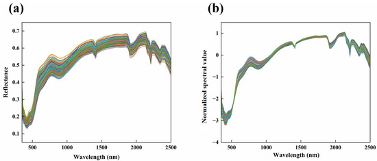
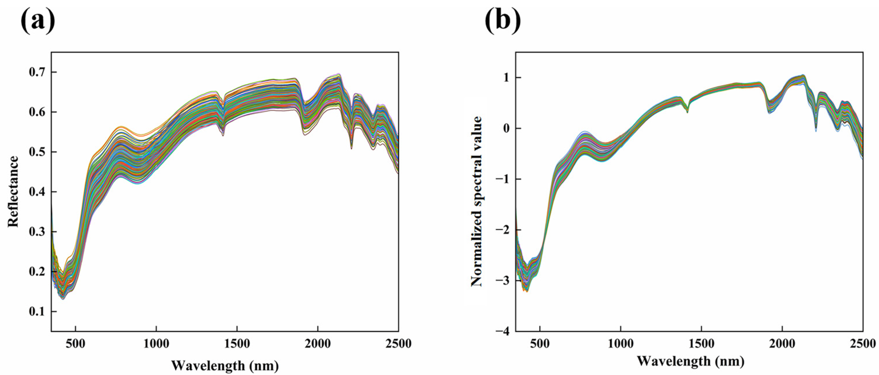
As shown in Figure 3a, after SG smoothing, the overall spectral curves exhibited broadly consistent trends, characterized by low reflectance in the visible region, a gradual increase with wavelength, relatively stable reflectance in the near-infrared and shortwave infrared regions, and distinct absorption features around 1400 nm, 1900 nm, and 2200 nm. SG smoothing reduced the random noise in the original spectra to some extent, making the overall curves more continuous and smoother. However, noticeable baseline differences and amplitude dispersion among samples remained, indicating that variations in surface conditions and scattering effects still influenced the spectral signals.
Figure 3.
(a) Spectral curve after SG smoothing; (b) Spectral curve after SG + SNV processing. Each colored line represents one of the 244 spectral observations obtained from the 61 mural plaster specimens.
As shown in Figure 3b, after SG smoothing followed by SNV transformation, the overall spectral characteristics were largely preserved, whereas baseline drift among samples was markedly reduced. In addition, the dispersion of the spectral curves was clearly lower than that in Figure 3a, particularly in the visible and near-infrared regions. These results indicate that SNV can effectively reduce scattering effects caused by differences in sample surface roughness, particle characteristics, and optical path variation, thereby improving the comparability of spectra among different samples.
3.2. Analysis of Wavelet Coefficient Curves at Different Decomposition Scales
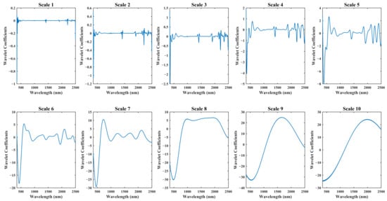
As shown in Figure 4, the SG + SNV-preprocessed spectra were decomposed into wavelet coefficients at 10 scales using CWT. As the decomposition scale increased, the absolute values of the wavelet coefficients gradually increased, and the curve patterns transitioned from high-frequency oscillations at low scales to smoother and more gradual variations at high scales, indicating a clear scale dependence in the representation of spectral information by CWT.
Figure 4.
Wavelet coefficient curves at different decomposition scales.
At Scale 1 to Scale 3, the wavelet coefficient curves showed relatively small overall fluctuations but frequent local oscillations. This suggests that low scale decomposition preserved more detailed information and was more sensitive to subtle local variations in the original spectra, but also retained more high-frequency noise components. As the scale increased from Scale 4 to Scale 7, local peak-valley structures became progressively clearer, and the characteristic variations in the visible, near-infrared, and shortwave infrared regions were more clearly expressed. This indicates that within this scale range, CWT was able to suppress high-frequency noise while still preserving local spectral shape information related to sample differences, thus showing good feature enhancement capability. When the scale further increased to Scale 8 to Scale 10, the wavelet coefficient curves became progressively smoother and local fluctuations decreased markedly. In particular, Scale 9 and Scale 10 exhibited slowly varying large-scale trends, with some subtle features being substantially weakened or even lost, indicating a certain degree of oversmoothing. Overall, the coefficient morphology demonstrated a gradual transition from detail-sensitive low-scale representations to increasingly smoothed high-scale representations. However, visual inspection of the coefficient curves alone was insufficient to identify an optimal CWT scale. The relative suitability of the ten scales was therefore determined quantitatively using nested PCC-SPA selection and specimen-grouped prediction performance.
3.3. Feature Selection
3.3.1. Pearson Correlation Analysis Between NaCl Content and Spectral Features
To characterize the overall scale-dependent relationships between NaCl content and the different spectral feature representations, a descriptive Pearson correlation analysis was conducted for SG, SG + SNV, and the ten CWT scales. The maximum absolute Pearson correlation coefficient was used to represent the strongest locally sensitive variable within each feature set, whereas the mean absolute Pearson correlation coefficient was used to characterize the overall level of correlation across all wavelengths. The resulting statistical summaries are presented in Table 2. This full-dataset descriptive analysis was independent of the nested feature-selection procedure used for predictive modeling; within the regression-model validation procedure, PCC screening was repeated using only the corresponding outer training specimens.
Table 2.
Maximum and Mean Absolute Pearson Correlation Coefficients between Sodium Chloride Content and SG, SG + SNV, and Wavelet Features.
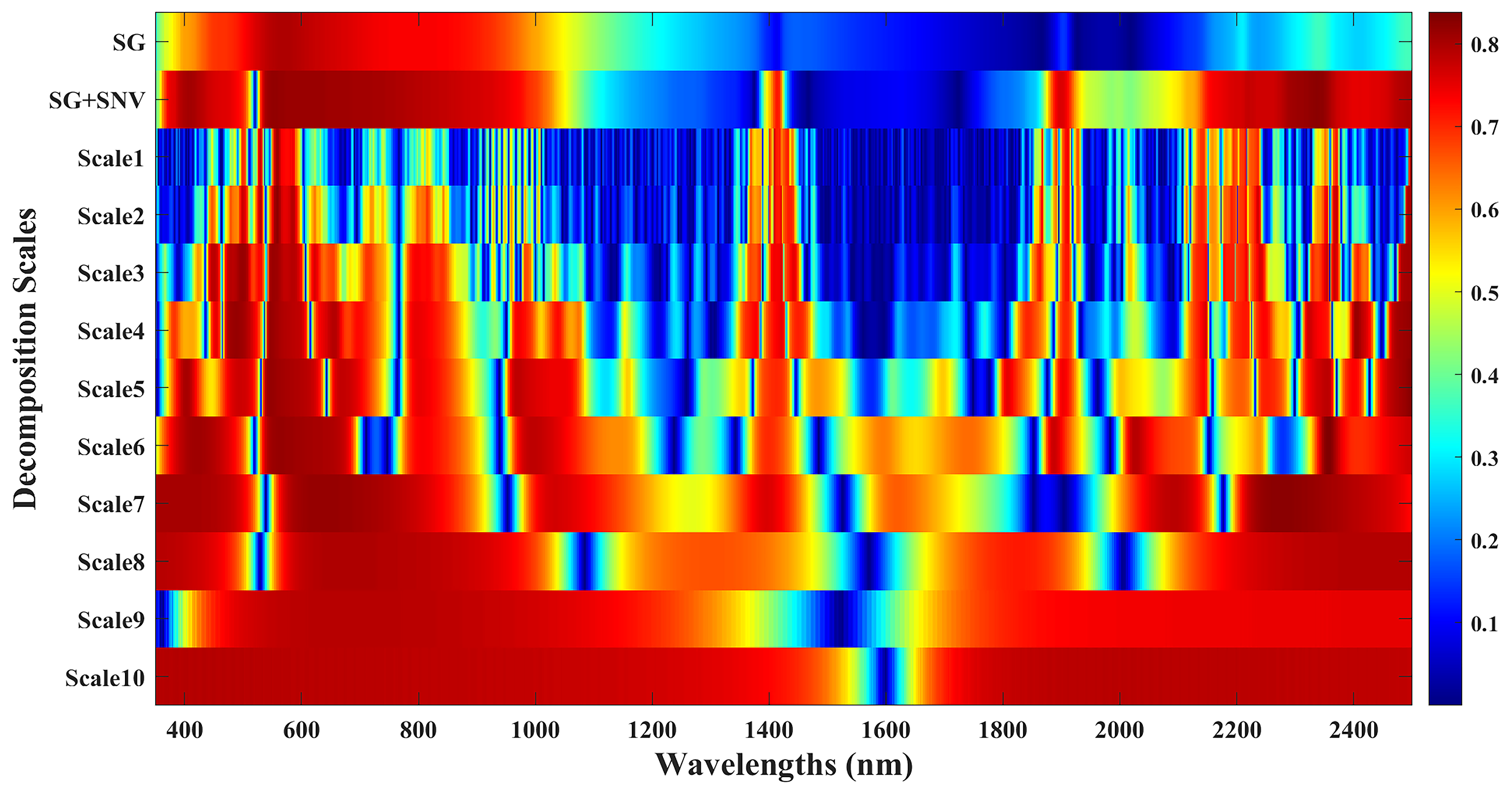
As shown in Table 2, the correlation structure changed markedly with CWT scale. The maximum absolute coefficient reached its highest value at Scale 6, whereas the mean absolute coefficient continued to increase toward the highest scales. This indicates that high-scale smoothing produced broad regions of neighboring coefficients with similar overall trends, but did not necessarily provide the most complementary multivariate feature subset. Therefore, univariate correlation strength alone was insufficient for determining the most suitable CWT scale.
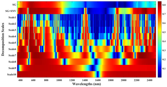
Figure 5 further illustrates the wavelength-dependent correlation patterns. Lower CWT scales produced relatively narrow and discontinuous high-correlation regions, whereas higher scales generated broader and smoother correlation structures. These patterns demonstrate that CWT scale influenced both the spatial extent and redundancy of the salt-related spectral response.
Figure 5.
Absolute Pearson correlations between NaCl content and SG/SG + SNV reflectance or CWT coefficients at different scales.
3.3.2. Fold-Wise Stability of Nested PCC-SPA Feature Selection
Because PCC-SPA selection was repeated independently within each outer training fold, both the number and the exact positions of the selected variables varied among the five folds. The average number of variables selected per fold was 6.6 for SG and 1.2 for SG + SNV. Across the CWT feature sets, the corresponding averages ranged from 1.2 to 5.2 variables per fold. For the representative CWT scales subsequently used in model comparison, Scale 2 retained 2–5 variables per fold, with an average of 3.2; Scale 6 retained 1–2 variables, with an average of 1.8; and Scale 7 retained 1–2 variables, with an average of 1.2. Scale 9 and Scale 10 showed larger fold-to-fold variation, with 1–12 and 1–20 selected variables, respectively.
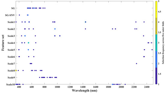
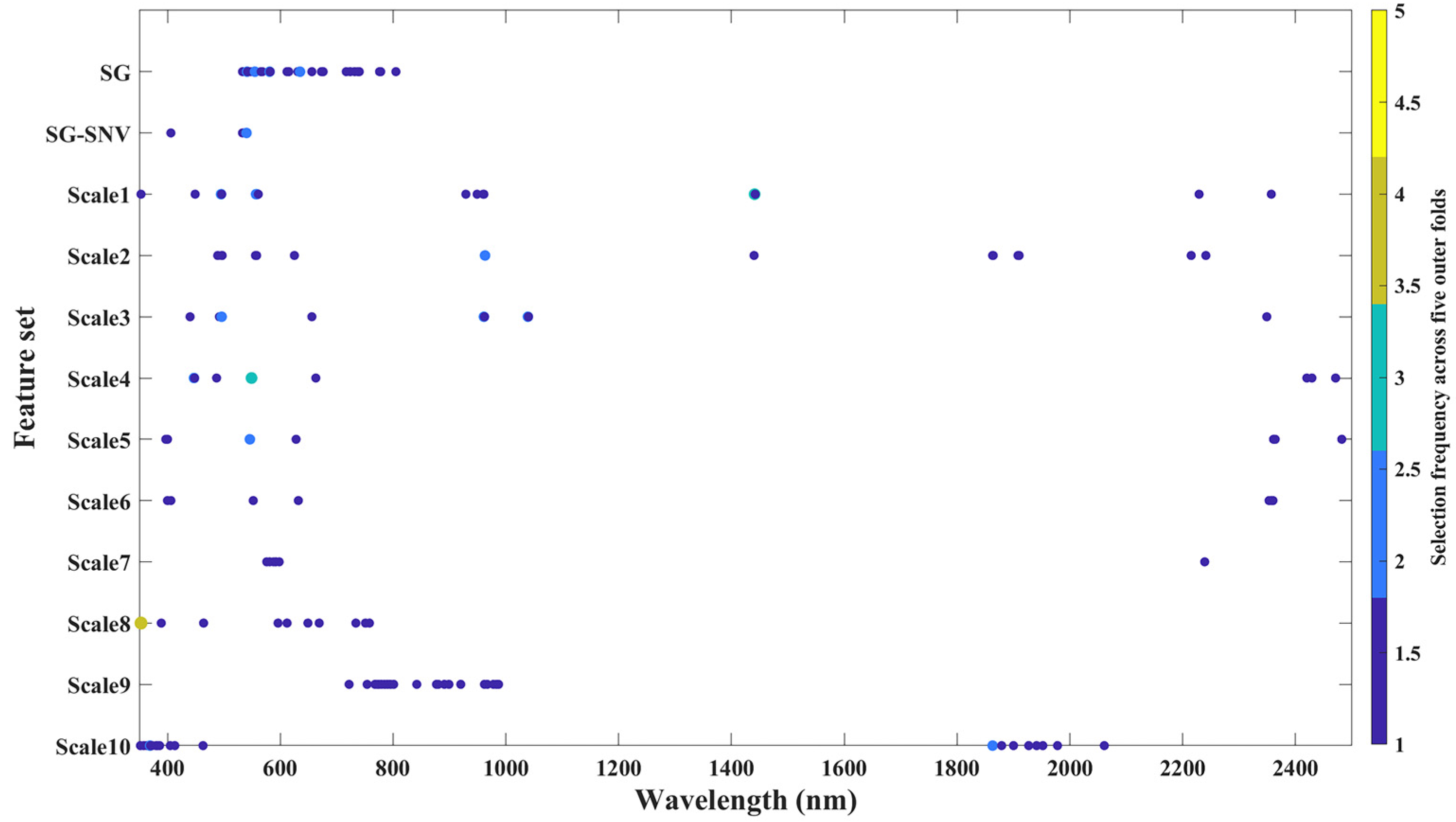
Figure 6 summarizes the fold-wise selection frequencies of the retained variables. Across the 12 feature representations, 167 feature-set-specific wavelength variables were retained at least once. Among these, 148 variables (88.6%) were selected in only one outer fold and 16 variables (9.6%) were selected in two folds. Only three variables were retained in at least three of the five folds: the Scale 1 coefficient at 1441 nm was selected in three folds, the Scale 4 coefficient at 549 nm was selected in three folds, and the Scale 8 coefficient at 353 nm was selected in four folds. No variable was retained in all five folds. These results indicate that exact-wavelength selection was sensitive to the composition of the outer training data and that selection stability was more evident at the level of broader spectral regions than at a single fixed wavelength.
Figure 6.
Fold-wise selection frequencies of wavelength variables retained by nested PCC-SPA for SG, SG + SNV, and the ten CWT scales. The color represents the number of outer training folds in which each scale-specific wavelength variable was selected.
Clear differences were also observed in the spectral distributions of the selected variables. Of the 33 SG selection events across the five folds, 32 occurred in the 350–799 nm region, whereas all six SG + SNV selection events occurred within the same visible range. In contrast, the CWT representations extended the selected variables into the near-infrared and short-wave infrared regions. Scale 2 contained seven visible-region, three 800–1799 nm, and six 1800–2500 nm selection events. Scale 6 contained four visible-region and five short-wave infrared selections, whereas Scale 7 contained five visible-region and one short-wave infrared selection. Thus, CWT expanded the spectral domain contributing to NaCl estimation beyond the predominantly visible-region variables retained from the conventional representations.
Because NaCl has weak and non-unique intrinsic absorption in the measured VNIR-SWIR range, the repeatedly selected regions should not be interpreted as chemically unique NaCl absorption bands. Visible-region variables may reflect changes in surface brightness, crystal coverage, roughness, and light scattering caused by salt crystallization, whereas near-infrared and short-wave infrared variables may reflect hydration-related behavior, hydroxyl-bearing plaster constituents, and salt–matrix interactions. The fold-wise recurrence therefore represents internal statistical relevance within the investigated mural plaster system rather than direct evidence of NaCl-specific absorption.
3.4. Comparison of Detection Results Among Different Models
The model and scale evaluations were conducted in two stages. In Stage 1, five regression approaches were compared using four representative feature sets: SG + SNV as the conventional preprocessing control, Scale 2 as a low-scale representation, Scale 6 as the scale with the highest maximum absolute PCC, and Scale 7 as an intermediate-to-high-scale representation with a relatively high mean absolute correlation. This stage was used to identify the strongest regression-model family. In Stage 2, the selected model family was evaluated using SG + SNV and all ten CWT scales to quantify CWT scale sensitivity and to identify the scales associated with the highest mean accuracy and the best accuracy–stability balance.
3.4.1. Comparison of Regression Models Using Representative Feature Sets
Using the four representative feature sets, PLSR, SVR, XGBoost, SVR-SSA, and XGBoost-SSA were evaluated under nested stratified specimen-grouped five-fold cross-validation. Specimen-level averaged performance was used as the primary comparison criterion, and the results are summarized in Table 3.
Table 3.
Specimen-level averaged prediction performance under nested stratified specimen-grouped five-fold cross-validation. RMSE and MAE are expressed in percentage points.
PLSR achieved specimen-level averaged R2 values ranging from 0.7576 to 0.7929. Scale 6 provided the strongest PLSR result, with R2 = 0.7929 ± 0.0947, RMSE = 0.3891 ± 0.0844 percentage points, and MAE = 0.2874 ± 0.0661 percentage points. This result shows that the performance of the linear model also varied with the spectral feature representation.
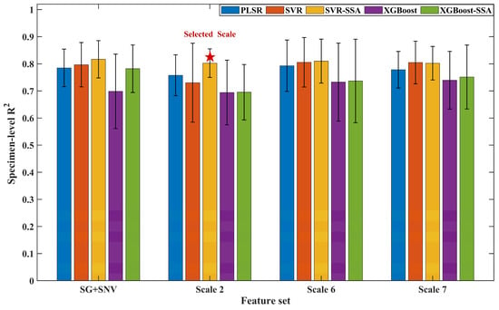
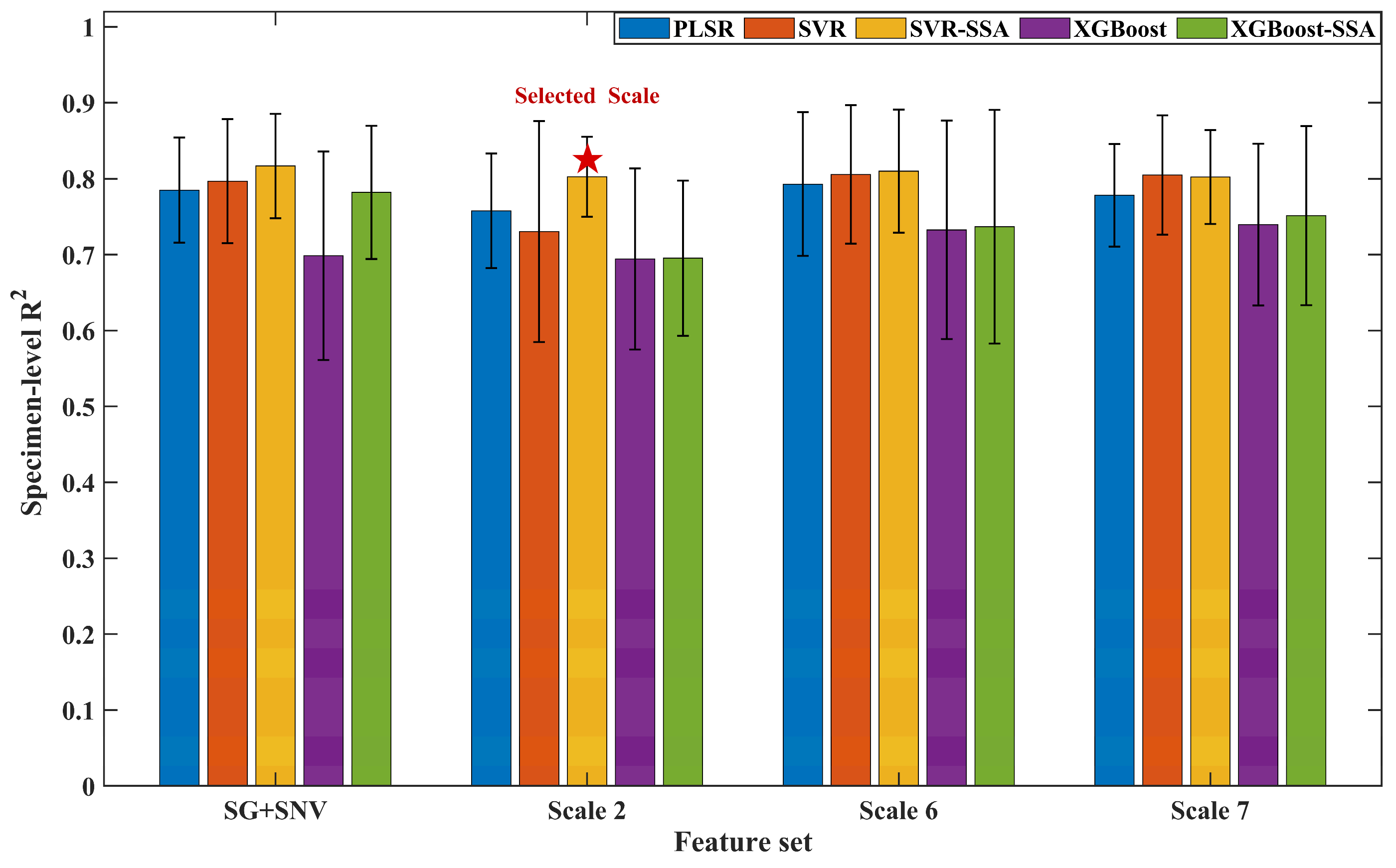
The influence of SSA optimization on SVR was feature-dependent. For SG + SNV, SSA increased the mean R2 from 0.7967 to 0.8167 and reduced the RMSE from 0.3886 to 0.3701 percentage points. The largest improvement occurred for Scale 2, for which the mean R2 increased from 0.7305 to 0.8026 and the RMSE decreased from 0.4408 to 0.3865 percentage points. Scale 6 showed a smaller improvement, whereas Scale 7 produced broadly comparable performance before and after optimization. Averaged across the four representative feature sets, SSA increased the mean R2 of SVR from 0.7845 to 0.8079 and reduced the mean RMSE from 0.3969 to 0.3790 percentage points.
Under SVR-SSA, the conventional SG + SNV representation and the intermediate-scale CWT representations produced closely comparable prediction performance. SG + SNV yielded the highest numerical mean R2 and the lowest numerical RMSE, whereas Scale 6 produced the lowest MAE of 0.2788 ± 0.0620 percentage points. These results identified SVR-SSA as the strongest model family and motivated its use in the complete CWT scale-sensitivity analysis.
SSA optimization also affected XGBoost in a feature-dependent manner. The largest improvement was observed for SG + SNV, whereas the changes for the CWT representations were smaller and less consistent. Overall, XGBoost-SSA remained less accurate than SVR-SSA under the current small-specimen and compact-feature conditions.
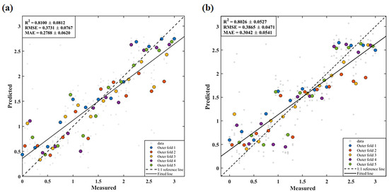
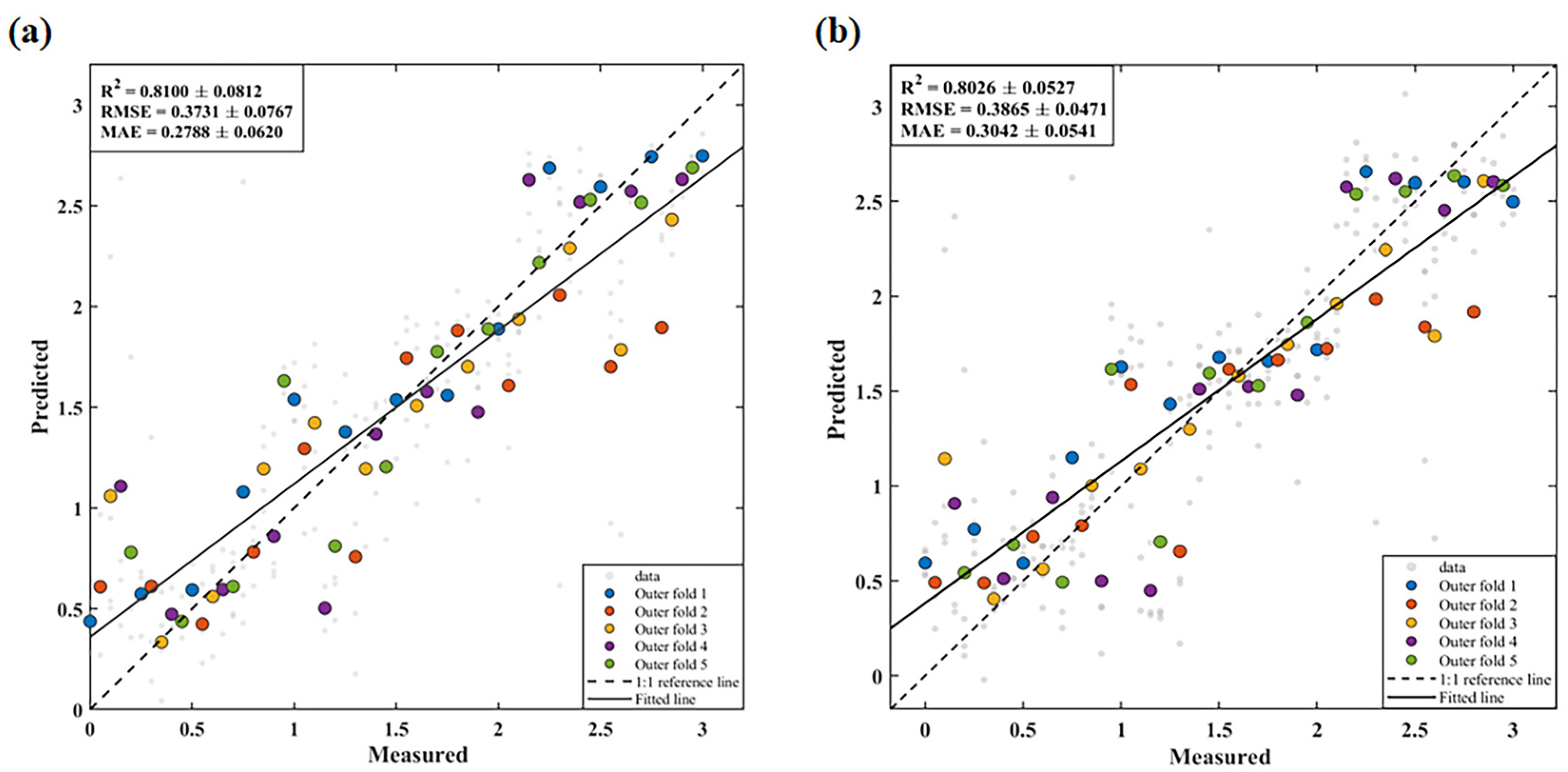
Figure 7 presents the out-of-fold predictions of the two representative CWT configurations identified from the complete scale-sensitivity analysis. Scale 6 represents the CWT configuration with the highest mean prediction accuracy, whereas Scale 2 represents the configuration with the best comprehensive accuracy–stability balance. The specimen-level averaged predictions of both configurations were generally distributed near the 1:1 reference line, demonstrating that useful NaCl-related predictive information was retained under different CWT scales.
Figure 7.
Out-of-fold prediction results of SVR-SSA using (a) Scale 6 CWT features and (b) Scale 2 CWT features under nested stratified specimen-grouped five-fold cross-validation. Gray points represent spectrum-level predictions, and colored circles represent specimen-level averaged predictions. Colors indicate the outer validation folds.
The overall comparison shown in Figure 8 further illustrates that the SSA-tuned SVR configurations generally achieved higher mean R2 values than the fixed-parameter SVR baseline, whereas the improvement obtained for XGBoost was more modest and varied among feature sets.
Figure 8.
Comparison of specimen-level averaged R2 values for the 20 model–feature combinations evaluated in Stage 1 under nested stratified specimen-grouped five-fold cross-validation. Error bars indicate the standard deviation across the five outer folds. The red star indicates Scale 2, which achieved the best comprehensive accuracy–stability rank among the CWT scales.
3.4.2. Scale Sensitivity Analysis of the SVR-SSA Model
Because Table 3 compared only four representative feature sets, SVR-SSA was further evaluated using SG + SNV and all ten CWT scales under the same nested stratified specimen-grouped five-fold cross-validation framework. This analysis was used to quantify the influence of CWT scale on mean prediction accuracy and fold-to-fold stability. The results are presented in Table 4.
Table 4.
Specimen-level averaged performance and comprehensive accuracy–stability ranking of SVR-SSA using SG + SNV and the ten CWT scales under nested stratified specimen-grouped five-fold cross-validation.
SG + SNV and several intermediate CWT scales yielded closely comparable prediction performance. SG + SNV produced a mean R2 of 0.8167 ± 0.0690 and an RMSE of 0.3701 ± 0.0636 percentage points. Among the CWT scales, Scale 6 achieved the highest mean accuracy, with R2 = 0.8100 ± 0.0812, RMSE = 0.3731 ± 0.0767 percentage points, and MAE = 0.2788 ± 0.0620 percentage points. Scale 6 therefore achieved nearly the same R2 and RMSE magnitude as SG + SNV while producing a lower MAE.
Scale 2 obtained the lowest comprehensive average rank of 3.50 because it combined competitive mean prediction performance with relatively low fold-to-fold variability. Therefore, Scale 6 was identified as the highest-accuracy CWT representation, whereas Scale 2 was identified as the most balanced CWT representation. The results demonstrate that CWT scale affected prediction accuracy, error characteristics, and partition stability, and that no single representation was uniformly superior under all evaluation criteria.
4. Discussion
4.1. Scale-Dependent Spectral Characteristics and CWT Modeling Performance
Pearson correlation analysis and multivariate prediction emphasized different aspects of the CWT representations. Scale 6 produced the highest maximum absolute correlation, whereas Scale 10 produced the highest mean absolute correlation. However, higher overall correlation did not directly translate into stronger predictive performance. Pearson correlation describes the marginal linear association between an individual wavelet coefficient and NaCl content, whereas multivariate prediction also depends on feature complementarity, redundancy, nonlinear model response, and partition stability. At higher scales, stronger smoothing can generate broad regions of neighboring coefficients with similar trends, increasing the mean correlation while simultaneously increasing redundancy.
The complete scale-sensitivity analysis further demonstrated that mean accuracy and fold-to-fold stability should be considered separately. Scale 6 achieved the highest mean CWT prediction accuracy and the lowest mean errors, whereas Scale 2 obtained the best comprehensive accuracy–stability rank. The relatively small differences among several intermediate scales indicate that the CWT representations provided a continuum of detail and smoothing rather than one universally optimal scale. Scale 6 preserved a favorable balance for minimizing average prediction error, whereas Scale 2 produced a more stable compromise across the five specimen partitions.
The predictive performance of Scale 6 was close in magnitude to that of the conventional SG + SNV representation, and Scale 6 produced a lower MAE. Therefore, CWT should not be interpreted solely as a procedure intended to exceed conventional preprocessing in every metric. Its principal value lies in introducing a scale dimension through which local spectral variations, prediction error, and model stability can be systematically investigated. This scale-resolved information cannot be obtained from a single SG + SNV representation.
Because PCC-SPA selection was repeated independently within each outer training fold, the exact selected variables varied across folds. Recurrently selected wavelength regions should therefore be interpreted as internally stable predictive regions rather than fixed or chemically unique NaCl markers. Visible-region variables may reflect salt-induced changes in surface brightness, crystal coverage, roughness, and scattering, whereas short-wave infrared variables may reflect hydration, hydroxyl-bearing plaster components, and salt–matrix interactions. These variables represent the combined optical response of NaCl crystallization and the investigated plaster matrix.
4.2. Predictive Performance of Different Models and the Role of SSA Optimization
The grouped comparison demonstrated that the effect of SSA optimization depended on both the regression algorithm and the spectral feature representation. For SVR, the largest gain occurred for Scale 2, where SSA increased the mean R2 by 0.0721 and reduced the RMSE by 0.0543 percentage points. SSA also improved the SG + SNV configuration, whereas the changes for Scale 6 were smaller and the Scale 7 results remained broadly comparable. Averaged across the four representative feature sets, SSA increased the mean R2 of SVR from 0.7845 to 0.8079 and reduced the mean RMSE from 0.3969 to 0.3790 percentage points.
The improvement obtained for XGBoost was less consistent. Although SSA substantially improved the SG + SNV configuration, only modest changes were observed for several CWT feature sets. The stronger overall performance of SVR-SSA indicates that kernel-parameter optimization was particularly effective under the present small-specimen and compact PCC-SPA feature conditions. By contrast, the more complex tree-based XGBoost model remained more sensitive to limited independent sample size despite its internal regularization and subsampling mechanisms.
The methodological contribution of this study lies in integrating fold-specific SSA hyperparameter optimization with conventional and multiscale spectral representations under a leakage-controlled nested specimen-grouped validation framework. Rather than evaluating SSA under only one selected preprocessing condition, the study quantified both the effectiveness of SSA and its dependence on input feature representation. The results indicate that SSA does not mechanically improve every feature-model combination; instead, it provides the greatest benefit when the predefined model parameters are poorly matched to the structure of the selected feature subset.
Table 5 compares the present work with representative hyperspectral or chemometric studies of mural salts and related materials. Direct numerical ranking should be interpreted cautiously because the studies differ in salt type, response variable, concentration range, sample preparation, RMSE units, and validation strategy. The contribution of the present study is therefore not limited to one maximum R2 value, but includes complete CWT-scale evaluation, fold-specific SSA optimization, training-fold-only PCC-SPA selection, and specimen-level evaluation of prediction stability.
Table 5.
Quantitative comparison with representative hyperspectral or chemometric methods for mural salt or salt-related material analysis.
Table 5 places the present results within the context of previous hyperspectral studies on mural salts and salt-related materials. Direct numerical ranking should be interpreted cautiously because these studies differed in salt type, response variable, concentration range, sample preparation, spectral processing, RMSE unit, and validation strategy. Guo et al. [36] and Dong et al. [38]. reported results from single calibration–validation partitions, whereas the present study used specimen-grouped five-fold cross-validation and retained all repeated spectra from the same physical specimen within one fold. The present R2 therefore represents the mean performance across multiple specimen partitions rather than the best result from one validation subset. In addition, the RMSE reported by Ren and Liu [37] was based on electrical conductivity and is not directly comparable with the percentage-point RMSE used for salt concentration in the present study. The main methodological contribution of the present work is the systematic comparison of CWT scales and nonlinear models together with specimen-level evaluation of prediction stability.
4.3. Applicability and Validation Scope for Authentic Mural Materials
The controlled plaster specimens isolated the spectral responses associated with NaCl concentration from major environmental interferences, providing a well-controlled basis for method development and model comparison. Authentic murals additionally contain pigments, mixed salts, heterogeneous minerals, aging products, variable moisture, contamination, and irregular surfaces. The next validation stage will extend the established framework to naturally aged and field-collected materials under these more complex conditions. The current single-salt model cannot establish chemical selectivity for NaCl when multiple salts coexist, and mixed-salt validation is therefore required. In authentic murals, aging, contamination, and irregular surfaces may introduce variable scattering, shadows, and background mixing; fixed measurement geometry, repeated spatial measurements, and representative field calibration may reduce these effects. During in situ acquisition, ambient-light interference should be controlled using a stable artificial light source or shading enclosure together with frequent white-reference and dark-current measurements.
The present internal validation included nested PCC screening, SPA subset selection, standardization, PLSR latent-variable selection, and SSA hyperparameter optimization within the outer training folds. This procedure reduced selection bias and provided a more realistic estimate of internal partition stability. Nevertheless, all outer folds originated from the same controlled experimental population. External validation using additional plaster compositions, naturally aged specimens, field-collected materials, and authentic mural surfaces is therefore required before chemical selectivity, robustness, and transferability can be established.
5. Conclusions
This study developed and evaluated an SSA-centered hyperspectral regression framework for estimating NaCl content in laboratory-prepared mural plaster specimens. CWT was used to construct multiscale spectral representations, and the complete feature-selection and model-optimization procedures were evaluated using nested stratified specimen-grouped five-fold cross-validation. The principal conclusions are as follows.
(1) The fully nested validation framework kept the four repeated spectra from each physical specimen within the same outer fold. PCC screening, SPA subset selection, standardization, PLSR latent-variable selection, and SSA hyperparameter optimization were conducted exclusively within the corresponding outer training folds. This procedure prevented held-out specimens from influencing feature selection or model tuning and provided an internally valid estimate of partition stability.
(2) SSA optimization improved the average predictive performance of SVR across the representative feature sets, although the magnitude of improvement depended on the input feature representation. The largest gain was observed for Scale 2, whereas Scale 6 showed a modest improvement and Scale 7 remained broadly unchanged after optimization. These results demonstrate that the value of SSA lies in its ability to adapt model hyperparameters to feature subsets with different dimensional, scale, and redundancy characteristics.
(3) SVR-SSA maintained high prediction capability under both conventional and multiscale feature representations. SG + SNV produced an R2 of 0.8167 ± 0.0690 and an RMSE of 0.3701 ± 0.0636 percentage points. Scale 6 CWT produced closely comparable values of R2 = 0.8100 ± 0.0812 and RMSE = 0.3731 ± 0.0767 percentage points, together with a lower MAE of 0.2788 ± 0.0620 percentage points. These results indicate complementary advantages among the different spectral representations rather than uniform superiority of one representation across all metrics.
(4) CWT revealed clear scale-dependent behavior in feature relevance, prediction error, and fold-to-fold stability. Scale 6 achieved the highest mean prediction accuracy among the CWT scales, whereas Scale 2 provided the best comprehensive accuracy–stability balance. Therefore, CWT contributed not only predictive variables but also a scale-resolved basis for understanding the indirect NaCl–plaster spectral response.
Overall, the results support the use of fold-specific SSA optimization for hyperspectral NaCl estimation and demonstrate the value of CWT for multiscale spectral characterization. The current conclusions are restricted to internally validated laboratory-prepared mural plaster specimens. External validation on additional plaster compositions, mixed-salt systems, naturally aged materials, and authentic mural surfaces remains necessary before field transferability can be established.
Supplementary Materials
The following supporting information can be downloaded at: https://www.mdpi.com/article/10.3390/chemosensors14080183/s1, Table S1. Fold-specific wavelengths and selection frequencies obtained from nested PCC-SPA feature selection for SG, SG + SNV, and the ten CWT scales.
Author Contributions
Methodology, data collection, formal analysis, investigation, and the writing of the original draft were performed by W.L. Writing—review and editing, and validation were done by S.L. Material preparation, project administration, and supervision were carried out by F.G., S.Z., X.P. and H.Z. All authors have read and agreed to the published version of the manuscript.
Funding
This research was funded by the Open Project of the Chinese Academy of Cultural Heritage, ‘Salt Spectral Response Mechanism and Quantitative Retrieval Method of Typical Temple Murals—Taking Cheng’en Temple in Beijing and Yiju Temple in Shanxi Province as Examples’, and the National Natural Science Foundation of China (Grant No. 42171356).
Institutional Review Board Statement
Not applicable.
Informed Consent Statement
Not applicable.
Data Availability Statement
The data presented in this study are not publicly available due to ongoing research and institutional data management restrictions. The data may be made available from the corresponding author upon reasonable request.
Acknowledgments
The authors would like to thank the laboratory staff for their assistance with sample preparation and hyperspectral data acquisition.
Conflicts of Interest
The authors declare no conflicts of interest. The funders had no role in the design of the study; in the collection, analyses, or interpretation of data; in the writing of the manuscript; or in the decision to publish the results.
Abbreviations
The following abbreviations are used in this manuscript:
| CWT | Continuous wavelet transform |
| SG | Savitzky–Golay |
| SNV | Standard normal variate |
| SPA | Successive projections algorithm |
| PCC | Pearson correlation coefficient |
| PLSR | Partial least squares regression |
| SVR | Support vector regression |
| RBF | Radial basis function |
| XGBoost | Extreme gradient boosting |
| SSA | Sparrow search algorithm |
| R2 | Coefficient of determination |
| RMSE | Root mean square error |
| MAE | Mean absolute error |
References
- Wang, Y.; Wu, X. Current Progress on Murals: Distribution, Conservation and Utilization. Herit. Sci. 2023, 11, 61. [Google Scholar] [CrossRef] [Scilit] [PubMed]
- Li, F.; Liu, H.; Yang, H.; Ayyamperumal, R.; Liu, Y. Influence of Water Vapor Sorption of NaCl-Na2SO4-Containing Mural Earthen Plaster and Preliminary Deterioration Analysis. Total Environ. Res. Themes 2023, 6, 100040. [Google Scholar] [CrossRef] [Scilit]
- Ren, Y.; Liu, F. Investigative Experiment on In-Situ Low-Temperature Crystallization Induction Time Measurement for Dunhuang Murals, Considering Porosity Factors. npj Herit. Sci. 2025, 13, 88. [Google Scholar] [CrossRef] [Scilit]
- Simonelli, G.; Sidoti, G.; Ruggiero, L.; Calia, A.; Quarta, G.; Aramini, F.; Mezzadri, P. The Use of Phosphonates to Inhibit Salt Crystallization: A Laboratory Study for the Sustainable Conservation of Mural Paintings in the Hypogea Context. Sustainability 2024, 16, 9745. [Google Scholar] [CrossRef] [Scilit]
- Guo, Z.Q.; Lyu, S.Q.; Hou, M.L. Estimation of the Soluble Salt Concentration in Murals Based on Spectral Transformation and Feature Extraction Modelling. J. Appl. Spectrosc. 2023, 90, 1123–1132. [Google Scholar] [CrossRef] [Scilit]
- Ren, Y.; Liu, F. The Spectral Inversion Model for Electrical Conductivity in Mural Plaster Following Phosphate Erosion Based on Fractional Order Differentiation and Novel Spectral Indices. Herit. Sci. 2024, 12, 286. [Google Scholar] [CrossRef] [Scilit]
- Tang, Y.; Li, F.; Yang, H.; Hu, Y.; Yu, K. A Transferable MMD-CWT Framework for Accurate Cross-Regional Prediction of Maize Leaf Nitrogen Using Hyperspectral Sensing. Eur. J. Agron. 2026, 177, 128092. [Google Scholar] [CrossRef] [Scilit]
- Yang, J.; Li, X.; Ma, X. Improving the Accuracy of Soil Organic Carbon Estimation: CWT-Random Frog-XGBoost as a Prerequisite Technique for In Situ Hyperspectral Analysis. Remote Sens. 2023, 15, 5294. [Google Scholar] [CrossRef] [Scilit]
- Yao, X.; Si, H.; Cheng, T.; Jia, M.; Chen, Q.; Tian, Y.; Zhu, Y.; Cao, W.; Chen, C.; Cai, J.; et al. Hyperspectral Estimation of Canopy Leaf Biomass Phenotype per Ground Area Using a Continuous Wavelet Analysis in Wheat. Front. Plant Sci. 2018, 9, 1360. [Google Scholar] [CrossRef] [Scilit] [PubMed]
- Cheng, X.; Feng, Y.; Guo, A.; Huang, W.; Cai, Z.; Dong, Y.; Guo, J.; Qian, B.; Hao, Z.; Chen, G.; et al. Detection of Rubber Tree Powdery Mildew from Leaf Level Hyperspectral Data Using Continuous Wavelet Transform and Machine Learning. Remote Sens. 2023, 16, 105. [Google Scholar] [CrossRef] [Scilit]
- Li, R.; Gao, M.; Xu, Z.; Wang, J.; Xie, X. Hyper-Spectral Estimation of Soil Organic Matter in Apple Orchard Based on CWT. IOP Conf. Ser. Earth Environ. Sci. 2021, 734, 012030. [Google Scholar] [CrossRef] [Scilit]
- Jahani, T.; Kashaninejad, M.; Ziaiifar, A.M.; Golzarian, M.; Akbari, N.; Soleimanipour, A. Effect of Selected Pre-Processing Methods by PLSR to Predict Low-Fat Mozzarella Texture Measured by Hyperspectral Imaging. Food Meas. 2024, 18, 5060–5072. [Google Scholar] [CrossRef] [Scilit]
- Zhu, H.; Yu, H.; Liang, S.; Wei, Y.; Zhang, L.; Huang, S. Prediction of Apple Quality Indicators Under Different Bagging Treatments Using Hyperspectral Imaging Integrated with a Stacking SDAE-PLSR-RR Deep Learning Model. J. Food Sci. 2025, 90, e70769. [Google Scholar] [CrossRef] [Scilit] [PubMed]
- Wan, L.; Zhou, W.; He, Y.; Wanger, T.C.; Cen, H. Combining Transfer Learning and Hyperspectral Reflectance Analysis to Assess Leaf Nitrogen Concentration across Different Plant Species Datasets. Remote Sens. Environ. 2022, 269, 112826. [Google Scholar] [CrossRef] [Scilit]
- Canero, F.M.; Rodriguez-Galiano, V.; Chabrillat, S. Evaluating Airborne Hyperspectral Scanner (AHS) for the Mapping of Soil Organic Matter and Clay in a Mediterranean Forest Ecosystem. CATENA 2025, 252, 108889. [Google Scholar] [CrossRef] [Scilit]
- Wong, C.Y.; Gilbert, M.E.; Pierce, M.A.; Parker, T.A.; Palkovic, A.; Gepts, P.; Magney, T.S.; Buckley, T.N. Hyperspectral Remote Sensing for Phenotyping the Physiological Drought Response of Common and Tepary Bean. Plant Phenomics 2023, 5, 0021. [Google Scholar] [CrossRef] [Scilit] [PubMed]
- Huang, L.; Liu, Y.; Huang, W.; Dong, Y.; Ma, H.; Wu, K.; Guo, A. Combining Random Forest and XGBoost Methods in Detecting Early and Mid-Term Winter Wheat Stripe Rust Using Canopy Level Hyperspectral Measurements. Agriculture 2022, 12, 74. [Google Scholar] [CrossRef] [Scilit]
- Ye, M.; Zhu, L.; Li, X.; Ke, Y.; Huang, Y.; Chen, B.; Yu, H.; Li, H.; Feng, H. Estimation of the Soil Arsenic Concentration Using a Geographically Weighted XGBoost Model Based on Hyperspectral Data. Sci. Total Environ. 2023, 858, 159798. [Google Scholar] [CrossRef] [Scilit] [PubMed]
- Wu, B.; Yang, K.; Li, Y.; He, J. Hyperspectral Inversion of Heavy Metal Copper Content in Corn Leaves Based on DRS–XGBoost. Sustainability 2023, 15, 16770. [Google Scholar] [CrossRef] [Scilit]
- Yu, H.; Hu, Y.; Qi, L.; Zhang, K.; Jiang, J.; Li, H.; Zhang, X.; Zhang, Z. Hyperspectral Detection of Moisture Content in Rice Straw Nutrient Bowl Trays Based on PSO-SVR. Sustainability 2023, 15, 8703. [Google Scholar] [CrossRef] [Scilit]
- Tan, K.; Liu, Q.; Chen, X.; Xia, H.; Yao, S. Estimation of Soybean Internal Quality Based on Improved Support Vector Regression Based on the Sparrow Search Algorithm Applying Hyperspectral Reflectance and Chemometric Calibrations. Agriculture 2024, 14, 410. [Google Scholar] [CrossRef] [Scilit]
- Gu, C.; Liu, H.; You, Y.; Zeng, Q.; Zhou, Z.; Song, M.; Shi, Y.; Tian, T. Hyperspectral Inversion of Leaf Nitrogen Content in Wheat by Integrating CWT-SPA Feature Optimization and XGBoost-SSA Model. Smart Agric. Technol. 2026, 13, 101765. [Google Scholar] [CrossRef] [Scilit]
- Wang, Q.; Wang, Y.; Smith, A.S. Atmospheric Paleoart: A Case Study of the Murals in the Paleozoological Museum of China. Geoconserv. Res. 2024, 7, 072409. [Google Scholar] [CrossRef]
- Li, Y.; Hu, X.; Xie, H.; Wu, R.; Zhang, Z.; Guo, Q.; Hokoi, S. The Impact of Cave Opening and Closure on Murals Hygrothermal Behavior in Cave 98 of Mogao Caves, China. Build. Environ. 2024, 256, 111502. [Google Scholar] [CrossRef] [Scilit]
- Arts, L.P.A.; Van Den Broek, E.L. The Fast Continuous Wavelet Transformation (fCWT) for Real-Time, High-Quality, Noise-Resistant Time–Frequency Analysis. Nat. Comput. Sci. 2022, 2, 47–58. [Google Scholar] [CrossRef] [Scilit] [PubMed]
- Zhang, M.; Li, W.; Zhang, L.; Jin, H.; Mu, Y.; Wang, L. A Pearson Correlation-Based Adaptive Variable Grouping Method for Large-Scale Multi-Objective Optimization. Inf. Sci. 2023, 639, 118737. [Google Scholar] [CrossRef] [Scilit]
- Canova, L.D.S.; Vallese, F.D.; Pistonesi, M.F.; De Araújo Gomes, A. An Improved Successive Projections Algorithm Version to Variable Selection in Multiple Linear Regression. Anal. Chim. Acta 2023, 1274, 341560. [Google Scholar] [CrossRef] [Scilit] [PubMed]
- Zhu, J.; Jin, Y.; Zhu, W.; Lee, D.K. VIS-NIR Spectroscopy and Environmental Factors Coupled with PLSR Models to Predict Soil Organic Carbon and Nitrogen. Int. Soil Water Conserv. Res. 2024, 12, 844–854. [Google Scholar] [CrossRef] [Scilit]
- Bargam, B.; Boudhar, A.; Kinnard, C.; Bouamri, H.; Nifa, K.; Chehbouni, A. Evaluation of the Support Vector Regression (SVR) and the Random Forest (RF) Models Accuracy for Streamflow Prediction under a Data-Scarce Basin in Morocco. Discov. Appl. Sci. 2024, 6, 306. [Google Scholar] [CrossRef] [Scilit]
- Li, J.; An, X.; Li, Q.; Wang, C.; Yu, H.; Zhou, X.; Geng, Y. Application of XGBoost Algorithm in the Optimization of Pollutant Concentration. Atmos. Res. 2022, 276, 106238. [Google Scholar] [CrossRef] [Scilit]
- Zhao, J.; Zhu, T.; Qiu, Z.; Li, T.; Wang, G.; Li, Z.; Du, H. Hyperspectral Prediction of Pigment Content in Tomato Leaves Based on Logistic-Optimized Sparrow Search Algorithm and Back Propagation Neural Network. J. Agric. Eng. 2023, 54, 1528. [Google Scholar] [CrossRef] [Scilit]
- Fan, B.; Zhu, R.; He, D.; Wang, S.; Cui, X.; Yao, X. Evaluation of Mutton Adulteration under the Effect of Mutton Flavour Essence Using Hyperspectral Imaging Combined with Machine Learning and Sparrow Search Algorithm. Foods 2022, 11, 2278. [Google Scholar] [CrossRef] [Scilit] [PubMed]
- Yan, Z.; Huang, J.; Xiang, K. Kernel Extreme Learning Machine Optimized by the Sparrow Search Algorithm for Hyperspectral Image Classification. arXiv 2022, arXiv:2204.00973. [Google Scholar] [CrossRef] [Scilit]
- Amjad, M.; Ahmad, I.; Ahmad, M.; Wróblewski, P.; Kamiński, P.; Amjad, U. Prediction of Pile Bearing Capacity Using XGBoost Algorithm: Modeling and Performance Evaluation. Appl. Sci. 2022, 12, 2126. [Google Scholar] [CrossRef] [Scilit]
- Demir, S.; Sahin, E.K. An Investigation of Feature Selection Methods for Soil Liquefaction Prediction Based on Tree-Based Ensemble Algorithms Using AdaBoost, Gradient Boosting, and XGBoost. Neural Comput. Appl. 2023, 35, 3173–3190. [Google Scholar] [CrossRef] [Scilit]
- Guo, Z.Q.; Lyu, S.Q.; Hou, M.L.; Huang, M. Hyperspectral Inversion of Soluble Salt Content in Mural Painting. Int. Arch. Photogramm. Remote Sens. Spat. Inf. Sci. 2022, XLIII-B2-2022, 793–800. [Google Scholar] [CrossRef] [Scilit]
- Ren, Y.; Liu, F. A Model for Inversion of Hyperspectral Characteristics of Phosphate Content in Mural Plaster Based on Fractional-Order Differential Algorithm. Sci. Rep. 2024, 14, 17898. [Google Scholar] [CrossRef] [Scilit] [PubMed]
- Dong, Q.; Lyu, S.; Hou, M.; Jin, Y.; Li, X. An Inversion Approach for Salt Content in Simulated Murals Based on Spectral Enhancement and Sample Partitioning. Int. Arch. Photogramm. Remote Sens. Spat. Inf. Sci. 2025, XLVIII-M-9–2025, 415–422. [Google Scholar] [CrossRef] [Scilit]
- Li, S.; Lyu, S.; Hou, M.; Lin, W.; Meng, F. Hyperspectral Prediction Model for Mixed Salts on the Surfaces of Temple Murals in Northern China Based on Simulated Samples. Int. Arch. Photogramm. Remote Sens. Spat. Inf. Sci. 2025, XLVIII-M-9–2025, 835–842. [Google Scholar] [CrossRef] [Scilit]

Disclaimer/Publisher’s Note: The statements, opinions and data contained in all publications are solely those of the individual author(s) and contributor(s) and not of MDPI and/or the editor(s). MDPI and/or the editor(s) disclaim responsibility for any injury to people or property resulting from any ideas, methods, instructions or products referred to in the content. |
© 2026 by the authors. Licensee MDPI, Basel, Switzerland. This article is an open access article distributed under the terms and conditions of the Creative Commons Attribution (CC BY) license.