Numerical Integral Transform Methods for Random Hyperbolic Models with a Finite Degree of Randomness

Abstract

This paper deals with the construction of numerical solutions of random hyperbolic models with a finite degree of randomness that make manageable the computation of its expectation and variance. The approach is based on the combination of the random Fourier transforms, the random Gaussian quadratures and the Monte Carlo method. The recovery of the solution of the original random partial differential problem throughout the inverse integral transform allows its numerical approximation using Gaussian quadratures involving the evaluation of the solution of the random ordinary differential problem at certain concrete values, which are approximated using Monte Carlo method. Numerical experiments illustrating the numerical convergence of the method are included.

1. Introduction

Analytic-numerical solutions of random mean square partial differential models have been treated recently using random integral transforms [1,2,3]. It is well-known [4] that the type of appropriated integral transform depends closely on the type of equation and initial/boundary conditions due to the properties of the operational calculus of the underlying integral transform. Important hyperbolic models of the telegraph type are relevant in wave propagation [5,6], signal analysis [7] and random walk theory [8]. In real problems, parameters, coefficients and initial/boundary conditions are subject to uncertainties, not only by error measurement but also due to heterogeneity of the media, or the lack of access to the measurement. The evaluation of microwave heating processes in ferrite materials [9] using the classical deterministic model gives inaccurate results because of the complication of the distribution within the oven and the fluctuation in dielectric properties of the material with respect to the density, temperature, moisture content and other elements. Since the seminal paper by Kac [10], several authors have treated telegraph equation with uncertainties with other objectives [11,12].

Efficient methods for solving numerically deterministic problems such as finite-difference methods become unsuitable for the random case because the computation of the expectation and the variance of the approximation stochastic process. This computational complexity arises from the operational random calculus involving big random matrices throughout the iterative levels of the discretization steps and the necessity to store the information of all the previous levels of the iteration process.

These drawbacks for solving random partial differential models, essentially of computational complexity, motives the search for non-iterative alternatives. The random integral transform approach previously quoted has two main steps: The first step is the transformation of the original random partial differential problem into a random ordinary differential system. The second step is the recovery of the solution of the original problem throughout the random inverse integral transform. At this point, the random Gaussian quadrature technique provides an easy expression involving evaluations at the zeros of the underlying family of orthogonal polynomials linked to the Gaussian quadrature. This approach allows the treatment of both cases: the first case where the explicit solution of the random transformed ordinary differential problem is available, as well as when one needs to solve numerically because the evaluation of the Gaussian quadrature rules is required only at concrete points.

In this paper, we address the numerical solution of random hyperbolic models of telegraph type. Section 3 deals with the random linear telegraph type problem

$$\begin{array}{ccc}\hfill u_{tt}(x,t)+2b{u}_t(x,t)+au(x,t)& =& c{u}_{xx}(x,t)+\varphi (x,t),x\in \mathbb{R},t>0,\hfill \end{array}$$

(1)

$$\begin{array}{ccc}\hfill u(x,0)& =& f_1\left(x\right),\hfill \end{array}$$

(2)

$$\begin{array}{ccc}\hfill u_t(x,0)& =& f_2\left(x\right),\hfill \end{array}$$

(3)

where the damping coefficient b, the reaction coefficient a and the diffusion coefficient c, all are random variables (r.v.’s). We also assume that source term $\varphi (x,t)$ and initial conditions $f_1\left(x\right)$ and $f_2\left(x\right)$ are mean square (m.s.) continuous stochastic processes (s.p.’s) with a finite degree of randomness [13,14], and absolutely integrable with respect to the spatial variable in the real line. In this problem, the random numerical approximation of the random inverse Fourier transform is performed using Gauss–Hermite quadrature rule.

Section 4 studies the random heterogeneous telegraph type problem

$$\begin{array}{ccc}\hfill u_{tt}(x,t)& =& {\left(k\left(x\right)u_x(x,t)\right)}_x+a\left(x\right)u(x,t)+\psi (x,t),x>0,t>0,\hfill \end{array}$$

(4)

$$\begin{array}{ccc}\hfill u(0,t)& =& g_1\left(t\right),\hfill \end{array}$$

(5)

$$\begin{array}{ccc}\hfill u_x(0,t)& =& g_2\left(t\right),\hfill \end{array}$$

(6)

$$\begin{array}{ccc}\hfill u(x,0)& =& g\left(x\right),\hfill \end{array}$$

(7)

where $a\left(x\right)$, $k\left(x\right)$, $\psi (x,t)$, $g_1\left(t\right)$, $g_2\left(t\right)$ and $g\left(x\right)$ are m.s. continuous s.p.’s with a finite degree of randomness, and absolutely integrable with respect to the time variable those depending on t. Here, the diffusivity coefficient $k\left(x\right)$ is also assumed to be positive and m.s. differentiable. In this section, we use random Gauss–Laguerre quadrature rules. Section 2 includes some preliminaries about the solution of random linear differential systems that are used in further sections [14]. The paper ends with a conclusion in Section 5.

2. Numerical Solution of Random Linear Differential Problems via Simulations

For the sake of clarity in the presentation, we begin this section recalling some definitions and results of [15].

Given a complete probability space, $(\Omega ,\mathcal{F},\mathbb{P})$, ${\mathrm{L}}_p^{m\times n}(\Omega )$ denotes the set of all random matrices $X={\left(x_{i,j}\right)}_{m\times n}$ (denoted by capital case letters) whose entries $x_{i,j}$ (denoted by lower case letters) are r.v.’s satisfying

$${∥x_{i,j}∥}_p={\left(\mathbb{E}\left[|x_{i,j}{|}^p\right]\right)}^{1/p}<+\infty ,p\ge 1,$$

(8)

that is, $x_{i,j}\in {\mathrm{L}}_p(\Omega )$, where $\mathbb{E}\left[·\right]$ denotes the expectation operator. The space of all random matrices together with the matrix p-norm, that is, $\left({\mathrm{L}}_p^{m\times n}(\Omega ),{\parallel ·\parallel }_p\right)$ defined as follows

$${∥X∥}_p=\sum _{i=1}^m\sum _{j=1}^n{∥x_{i,j}∥}_p,\mathbb{E}\left[|x_{i,j}{|}^p\right]<+\infty ,$$

(9)

is a Banach space. Note that, in the case $m=n=1$, both norms are the same and $({\mathrm{L}}_p^{1\times 1}(\Omega )\equiv {\mathrm{L}}_p(\Omega ),{∥·∥}_p)$ represents the Banach space of real r.v.’s verifying Equation (8). The definition of matrix p-norm in Equation (9) can be extended to matrix s.p.’s $X\left(t\right)={\left(x_{i,j}\left(t\right)\right)}_{m\times n}$ of ${\mathrm{L}}_p^{m\times n}(\Omega )$ where now each entry $x_{i,j}\left(t\right)$ is a s.p., that is a r.v. for each t. We say that a matrix s.p. $X\left(t\right)$ lies in ${\mathrm{L}}_p^{m\times n}(\Omega )$ if ${\left(x_{i,j}\left(t\right)\right)}_{m\times n}\in {\mathrm{L}}_p(\Omega )$ for every $1\le i\le m$ and $1\le j\le n$. The definitions of continuity, differentiability and integrability of matrix s.p.’s lying in ${\mathrm{L}}_p^{m\times n}(\Omega )$ follow in a straightforwardly manner using matrix p-norm in Equation (9). The cases $p=2$ and $p=4$ correspond to the so-called mean square (m.s.) and mean fourth (m.f.) convergence, respectively. Specifically, when dealing with random differential equations, the reference space is ${\mathrm{L}}_2^{m\times n}(\Omega )$ ($p=2$) because in practise most r.v.’s have finite variance. However, the space ${\mathrm{L}}_4^{m\times n}(\Omega )$ ($p=4$), ${\mathrm{L}}_4^{m\times n}(\Omega )\subset {\mathrm{L}}_2^{m\times n}(\Omega )$, is also used in order to legitimize some mean square operational rules. Let us consider the random vector initial value problem (IVP)

$$Y^{\prime }\left(s\right)=L\left(s\right)Y\left(s\right),Y\left(0\right)=Y_0,s>0,$$

(10)

where $L\left(s\right)\in L_{2p}^{n\times n}(\Omega )$ is a matrix s.p. and $Y_0\in L_{2p}^{n\times 1}(\Omega )$, being $L\left(s\right)$$2p$-locally absolutely integrable, that is ${\int }_0^T{\parallel L\left(s\right)\parallel }_{2p}\mathrm{ds}<+\infty$. Assume that the random system in Equation (10) is random $2p$-regular, $p\ge 1$, in the sense of Definition 3, page 943, of [15], and let ${\Phi }_L(s;0)$ be the random fundamental matrix solution of Equation (10) satisfying

$${\Phi }_L^{\prime }(s;0)=L\left(s\right){\Phi }_L(s;0);{\Phi }_L(0;0)=I_n,$$

(11)

being $I_n$ the identity matrix of size n.

If $B\left(s\right)$ lies in $L_{2p}^{n\times 1}(\Omega )$ and is $2p$-integrable, with previous hypothesis on the random problem in Equation (10) and assuming that the entries of matrix s.p. $L\left(s\right)={\left({\ell }_{i,j}\left(s\right)\right)}_{n\times n}$ satisfies the moment condition of [15] for every $s>0$, that is

$$\mathbb{E}\left[{\left|{\ell }_{i,j}\left(s\right)\right|}^r\right]\le m_{i,j}{\left(h_{i,j}\right)}^r<+\infty ,\forall r\ge 0,\forall i,j:1\le i,j\le m,$$

(12)

then, by Theorem 1, page 944, of [15], the solution of the non-homogeneous problem

$$X^{\prime }\left(s\right)=L\left(s\right)X\left(s\right)+B\left(s\right),X\left(0\right)=Y_0,$$

(13)

is given by

$$X\left(s\right)={\Phi }_L(s;0)Y_0+{\Phi }_L(s;0){\int }_0^s{\Phi }_L^{-1}(v;0)B\left(v\right)\mathrm{dv}.$$

(14)

In particular, if $L\left(s\right)=L$ is a constant random matrix, see Section 3 of [16], the corresponding solution in Equation (14) of Equation (13) can be written as

$$X\left(s\right)=e^{Ls}\left\{Y_0+{\int }_0^s{e}^{-Lv}B\left(v\right)\mathrm{dv}\right\}.$$

(15)

Note that the m.s. solution of Equation (13), given by Equation (14), is not available, apart from very limited cases, see Example 5 of [15], because the random fundamental matrix ${\Phi }_L(s;0)$ is not known.

This motivates the search of alternative approximations via simulations, the so called Monte Carlo approach [17], that provides the expectation $\mathbb{E}\left[X\right(s\left)\right]$ throughout the average of an appropriate number of realizations $\omega \in \Omega$ of the deterministic problem

$$X^{\prime }(s,\omega )=L(s,\omega )X(s,\omega )+B(s,\omega ),X(0,\omega )=Y_0\left(\omega \right).$$

(16)

For the sake of convenience, we introduce an interesting example with known exact solution that is used below for solving a random hyperbolic problem.

Example 1.

Let $m\left(s\right)$, $n\left(s\right)$, and $q\left(s\right)$ be $2p$-continuous s.p.’s and let ${[y_1,y_2]}^T$ be a r.v. in $L_{2p}^{2\times 1}(\Omega )$. Assume that $n\left(s\right)$ and $q\left(s\right)$ satisfy the moment condition in Equation (12) for each s. Consider the random initial value problem in $L_{2p}^{2\times 1}(\Omega )$.

$$X^{\prime }\left(s\right)=\left[\begin{array}{cc}0& 1\\ n\left(s\right)& q\left(s\right)\end{array}\right]X\left(s\right)+\left[\begin{array}{c}0\\ m\left(s\right)\end{array}\right],X\left(0\right)=\left[\begin{array}{c}{y}_1\\ y_2\end{array}\right],$$

(17)

with

$$\begin{array}{c}\hfill \left.\begin{array}{c}n\left(s\right)=n(s;a,b)=-e^{(b-a)s},q\left(s\right)=q(s;b)=b,\hfill \\ m\left(s\right)=m(s;a,b)=1+(a-b)(a-2b)e^{(a-b)s},\hfill \\ y_1=1;y_2=y_2(a,b)=a-b,\hfill \end{array}\right\}\end{array}$$

(18)

where a is the truncated Gaussian r.v., $a\sim N_{[0.9,1.1]}(1,0.05)$, and b is the truncated beta r.v., $b\sim Bet{a}_{[0.1,0.8]}(2,0.25)$. Both r.v.’s, a and b, are independent.

It is easy to check that the exact m.s. solution of the test random problem in Equations (17) and (18) is given by

$$X\left(s\right)=\left[\begin{array}{c}{e}^{(a-b)s}\hfill \\ (a-b)e^{(a-b)s}\hfill \end{array}\right]=e^{(a-b)s}\left[\begin{array}{c}1\\ a-b\end{array}\right].$$

(19)

The expectation and the standard deviation of the random vector exact solution s.p. in Equation (19) at $s=1$, denoted by $X\left(1\right)={[x_1\left(1\right),x_2\left(1\right)]}^T$, take the following values

$$\begin{array}{ccc}\hfill \mathbb{E}\left[X\right(1\left)\right]& =& {\left[\mathbb{E}\left[x_1\left(1\right)\right],\mathbb{E}\left[x_2\left(1\right)\right]\right]}^T={[1.52728,0.671897]}^T\hfill \end{array}$$

(20)

$$\begin{array}{ccc}\hfill \sqrt{\mathrm{Var}\left[X\right(1\left)\right]}& =& {\left[\sqrt{\mathrm{Var}\left[x_1\left(1\right)\right]},\sqrt{\mathrm{Var}\left[x_2\left(1\right)\right]}\right]}^T={[0.284533,0.43069]}^T.\hfill \end{array}$$

(21)

Now, we illustrate and compare the numerical approximations with the exact solutions for the unfavorable and usual case when the solution s.p. of a random system of the type in Equation (17) is not available because the random fundamental matrix ${\Phi }_L(s;0)$ is not known. The search of alternative approximations is made via Monte Carlo approach, as we have just commented in this Section. Firstly, we consider in the system in Equations (17) and (18), for both r.v.’s, a and b, a different number of realizations $K_0={10}^4$, $K_1=2\times {10}^4$, $K_2=4\times {10}^4$, $K_3=8\times {10}^4$ and $K_4=1.6\times {10}^5$ for fixed value of s, obtaining $K_i$, $i=0,\dots ,4$, deterministic numerical solutions, denoted by $\overline{X}\left(s\right)={[{\overline{x}}_1\left(s\right),{\overline{x}}_2\left(s\right)]}^T$. Then, for a fixed realization $K_i$ and taking the average of the $K_i$ numerical solutions obtained, we compute the expectation ${\mathbb{E}}_{MC}^{K_i}\left[\overline{X}\left(1\right)\right]$. In a similar way, we compute the standard deviation $\sqrt{{\mathrm{Var}}_{MC}^{K_i}\left[\overline{X}\left(1\right)\right]}$ for a fixed realization $K_i$. Table 1, Table 2 and Table 3 include all these values together with the absolute errors and the numerical convergence ratios for a number $K_i$ of realizations, computed by

$$\begin{array}{ccc}\hfill {\mathit{ErrAbs}}_{{\mathbb{E}}_{MC}^{K_i}\left(s\right)}& =& \left|{\mathbb{E}}_{MC}^{K_i}\left[{\overline{x}}_j\left(s\right)\right]-\mathbb{E}\left[x_j\left(s\right)\right]\right|,j=1,2,\hfill \end{array}$$

(22)

$$\begin{array}{ccc}\hfill {\mathit{ErrAbs}}_{\sqrt{{\mathrm{Var}}_{MC}^{K_i}\left(s\right)}}& =& \left|\sqrt{{\mathrm{Var}}_{MC}^{K_i}\left[{\overline{x}}_j\left(s\right)\right]}-\sqrt{\mathrm{Var}\left[x_j\left(s\right)\right]}\right|,j=1,2,\hfill \end{array}$$

(23)

$$\begin{array}{ccc}\hfill {\mathit{ratio}}_{{\mathbb{E}}_{MC}^{K_{i-1}{K}_i}\left(s\right)}& =& \frac{\left|{\mathbb{E}}_{MC}^{K_{i-1}}\left[{\overline{x}}_j\left(s\right)\right]-\mathbb{E}\left[x_j\left(s\right)\right]\right|}{\left|{\mathbb{E}}_{MC}^{K_i}\left[{\overline{x}}_j\left(s\right)\right]-\mathbb{E}\left[x_j\left(s\right)\right]\right|},j=1,2,\hfill \end{array}$$

(24)

$$\begin{array}{ccc}\hfill {\mathit{ratio}}_{\sqrt{{\mathrm{Var}}_{MC}^{K_{i-1}{K}_i}\left(s\right)}}& =& \frac{\left|\sqrt{{\mathrm{Var}}_{MC}^{K_{i-1}}\left[{\overline{x}}_j\left(s\right)\right]}-\sqrt{\mathrm{Var}\left[x_j\left(s\right)\right]}\right|}{\left|\sqrt{{\mathrm{Var}}_{MC}^{K_i}\left[{\overline{x}}_j\left(s\right)\right]}-\sqrt{\mathrm{Var}\left[x_j\left(s\right)\right]}\right|}j=1,2,\hfill \end{array}$$

(25)

respectively. Table 1 and Table 2 show the values of both the expectation and the standard deviation of the numerical approximations at $s=1$ obtained when simulations via Monte Carlo are used considering a different number of realizations $K_i$ of both r.v.’s a and b in the system in Equations (17) and (18). Using the definition of the numerical convergence ratio for a number $K_i$ of realizations, given by Equations (24) and (25), the expected numerical convergence of both the expectation and the standard deviation of the numerical solutions of the Monte Carlo simulated problems to those of the exact random solution is shown. Although the convergence provided by Monte Carlo method is slow, it is a useful tool to manage the high computational problem. Table 1 and Table 2 show the good approximations to the exact values, $\mathbb{E}\left[x_j\left(s\right)\right]$ and $\sqrt{\mathrm{Var}\left[x_j\left(s\right)\right]}$, $j=1,2$, obtained by Monte Carlo method for $K=1.6\times {10}^5$ realizations, although the value of parameter s increases.

Table 1. Approximate values of the expectations, ${\mathbb{E}}_{MC}^{K_i}\left[{\overline{x}}_j\left(1\right)\right]$, their absolute errors, ${\mathrm{ErrAbs}}_{{\mathbb{E}}_{MC}^{K_i}\left(1\right)}$ (Equation (22)), and the numerical convergence ratios, ${\mathrm{ratio}}_{{\mathbb{E}}_{MC}^{K_{i-1}{K}_i}\left(1\right)}$ (Equation (24)), at $s=1$ for each component $j=1,2$ of the approximate vector solution of Equations (17) and (18) obtained by Monte Carlo method, $\overline{X}\left(1\right)=[{\overline{x}}_1\left(1\right),{\overline{x}}_2\left(1\right)]$, considering consecutive simulations $K_i$, $i=0,\cdots ,4$.

		${\mathbb{E}}_{\mathbf{MC}}^{{\mathit{K}}_{\mathit{i}}}\left[{\overline{\mathit{x}}}_{\mathit{j}}\left(1\right)\right]$	${\mathbf{ErrAbs}}_{{\mathbb{E}}_{\mathbf{MC}}^{{\mathit{K}}_{\mathit{i}}}\left(1\right)}$	${\mathbf{ratio}}_{{\mathbb{E}}_{\mathbf{MC}}^{{\mathit{K}}_{\mathit{i}-1}{\mathit{K}}_{\mathit{i}}}\left(1\right)}$
$K_0={10}^4$	$j=1$	$1.52545$	$1.82301e-03$	−
	$j=2$	$0.669022$	$2.87531e-03$	−
$K_1=2\times {10}^4$	$j=1$	$1.52640$	$8.72148e-04$	$2.09025$
	$j=2$	$0.67048$	$1.41528e-03$	$2.03162$
$K_2=4\times {10}^4$	$j=1$	$1.52826$	$9.86689e-04$	$0.88391$
	$j=2$	$0.67354$	$1.63892e-03$	$0.86355$
$K_3=8\times {10}^4$	$j=1$	$1.52568$	$1.59686e-03$	$0.61789$
	$j=2$	$0.66951$	$2.38523e-03$	$0.68711$
$K_4=1.6\times {10}^5$	$j=1$	$1.52708$	$2.00882e-04$	$7.94925$
	$j=2$	$0.67160$	$2.96101e-04$	$8.05546$

Table 2. Approximate values of the standard deviations, $\sqrt{{\mathrm{Var}}_{MC}^{K_i}\left[{\overline{x}}_j\left(1\right)\right]}$, their absolute errors, ${\mathrm{ErrAbs}}_{\sqrt{{\mathrm{Var}}_{MC}^{K_i}\left(1\right)}}$ (Equation (22)), and the numerical convergence ratios, ${\mathrm{ratio}}_{\sqrt{{\mathrm{Var}}_{MC}^{K_{i-1}{K}_i}\left(1\right)}}$ (Equation  (25)), at $s=1$ for each component $j=1,2$ of the approximate vector solution of Equations (17) and (18) obtained by Monte Carlo method, $\overline{X}\left(1\right)=[{\overline{x}}_1\left(1\right),{\overline{x}}_2\left(1\right)]$, considering consecutive simulations $K_i$, $i=0,\cdots ,4$.

		$\sqrt{{\mathbf{Var}}_{\mathbf{MC}}^{{\mathit{K}}_{\mathit{i}}}\left[{\overline{\mathit{x}}}_{\mathit{j}}\left(1\right)\right]}$	${\mathbf{ErrAbs}}_{\sqrt{{\mathbf{Var}}_{\mathbf{MC}}^{{\mathit{K}}_{\mathit{i}}}\left(1\right)}}$	${\mathbf{ratio}}_{\sqrt{{\mathbf{Var}}_{\mathbf{MC}}^{{\mathit{K}}_{\mathit{i}-1}{\mathit{K}}_{\mathit{i}}}\left(1\right)}}$
$K_0={10}^4$	$j=1$	$0.28309$	$1.44459e-03$	−
	$j=2$	$0.42914$	$1.54728e-03$	−
$K_1=2\times {10}^4$	$j=1$	$0.28352$	$1.00834e-03$	$1.43264$
	$j=2$	$0.42916$	$1.52672e-03$	$1.01346$
$K_2=4\times {10}^4$	$j=1$	$0.28609$	$1.55768e-03$	$0.64733$
	$j=2$	$0.43368$	$2.98663e-03$	$0.51119$
$K_3=8\times {10}^4$	$j=1$	$0.28377$	$7.61522e-04$	$2.04548$
	$j=2$	$0.42931$	$1.38278e-03$	$2.15987$
$K_4=1.6\times {10}^5$	$j=1$	$0.28453$	$2.50041e-06$	$304.559$
	$j=2$	$0.43082$	$1.32738e-04$	$10.4173$

Table 3. Exact values of the expectation, $\mathbb{E}\left[x_j\left(s\right)\right]$, and the standard deviation, $\sqrt{\mathrm{Var}\left[x_j\left(s\right)\right]}$, for each component $j=1,2$, of the random vector solution in Equation (19). The approximate values of both the expectations and the standard deviations, ${\mathbb{E}}_{MC}^K\left[{\overline{x}}_j\left(s\right)\right]$ and $\sqrt{{\mathrm{Var}}_{MC}^K\left[{\overline{x}}_j\left(s\right)\right]}$, respectively, and their absolute errors, ${\mathrm{ErrAbs}}_{{\mathbb{E}}_{MC}^K\left(s\right)}$ (Equation (22)) and ${\mathrm{ErrAbs}}_{\sqrt{{\mathrm{Var}}_{MC}^K\left(s\right)}}$ (Equation (23)) were computed by Monte Carlo method considering $K=1.6\times {10}^5$ simulations at different values of the parameter $s=\left\{0.5,1,1.5,2\right\}$.

		$\mathbb{E}\left[{\mathit{x}}_{\mathit{j}}\left(\mathit{s}\right)\right]$	${\mathbb{E}}_{\mathit{M}\mathit{C}}^{\mathit{K}}\left[{\overline{\mathit{x}}}_{\mathit{j}}\left(\mathit{s}\right)\right]$	${\mathbf{ErrAbs}}_{{\mathbb{E}}_{\mathbf{MC}}^{\mathit{K}}\left(\mathit{s}\right)}$	$\sqrt{\mathbf{Var}\left[{\mathit{x}}_{\mathit{j}}\left(\mathit{s}\right)\right]}$	$\sqrt{{\mathbf{Var}}_{\mathbf{MC}}^{\mathit{K}}\left[{\overline{\mathit{x}}}_{\mathit{j}}\left(\mathit{s}\right)\right]}$	${\mathbf{ErrAbs}}_{\sqrt{{\mathbf{Var}}_{\mathbf{MC}}^{\mathit{K}}\left(\mathit{s}\right)}}$
	$j=1$	$1.23086$	$1.23078$	$7.83976e-05$	$0.11073$	$0.11070$	$3.23642e-05$
$s=0.5$
	$j=2$	$0.52105$	$0.52085$	$1.97325e-04$	$0.27619$	$0.27618$	$1.52591e-05$
	$j=1$	$1.52728$	$1.52708$	$2.00882e-04$	$0.28453$	$0.28453$	$2.50041e-06$
$s=1$
	$j=2$	$0.67190$	$0.671601$	$2.96101e-04$	$0.43069$	$0.43082$	$1.32738e-04$
	$j=1$	$1.91133$	$1.91095$	$3.78171e-04$	$0.55336$	$0.55348$	$1.2166e-04$
$s=1.5$
	$j=2$	$0.874369$	$0.873953$	$4.16073e-04$	$0.66385$	$0.66419$	$3.3551e-04$
	$j=1$	$2.41353$	$2.41291$	$6.20018e-04$	$0.96546$	$0.96583$	$3.70421e-04$
$s=2$
	$j=2$	$1.14844$	$1.14788$	$5.55237e-04$	$1.01592$	$1.01649$	$5.69849e-04$

Computations were carried out by Mathematica${}^{\copyright }$ software version 11.3.0.0 [18] for Windows 10Pro (64-bit) Intel(R) Core(TM) i7-7820X CPU, 3.60 GHz 8 kernels. The timings (CPU time spent in the Wolfram Language kernel) for $K=1.6\times {10}^5$ and $s=1.5$ in Table 3 correspond to the most expensive scenario. They  were $86.25$ s for the generation of these K realizations of both r.v.’s a and b, and $174.047$ s to obtain the approximations of both the expectation and the standard deviation in Table 3.

3. Gauss–Hermite Solution of Random Telegraph Model

In this section, we construct numerical solution of the random telegraph model in Equations (1)–(3) in two-stages. Firstly, using the Fourier exponential transform, an infinite integral form solution of the theoretical solution is obtained. Then, using random Gauss–Hermite quadrature formulae a random numerical solution is represented that is further computer by means of Monte Carlo simulations.

Let $u(x,t)$ be the theoretical solution s.p. of the random problem in Equations (1)–(3), and let

$$U\left(t\right)\left(\xi \right)=\mathfrak{F}\left[u(·,t)\right]\left(\xi \right)=\frac{1}{\sqrt{2\pi }}{\int }_{-\infty }^{+\infty }u(x,t)e^{-ix\xi }\mathrm{dx},$$

(26)

be the Fourier exponential transform of the one-variable s.p. $u(·,t)$, for a fixed time t. Using the properties of the random Fourier exponential (see [1]), we have

$$\begin{array}{ccc}\hfill \mathfrak{F}\left[u_{xx}(·,t)\right]\left(\xi \right)& =& -{\xi }^2\mathfrak{F}\left[u(·,t)\right]\left(\xi \right)=-{\xi }^{2}U\left(t\right)\left(\xi \right),\hfill \end{array}$$

(27)

$$\begin{array}{ccc}\hfill \mathfrak{F}\left[u_t(·,t)\right]\left(\xi \right)& =& \frac{d}{dt}\left(\mathfrak{F}\left[u\right(·,t\left)\right]\right)\left(\xi \right)=\frac{d}{dt}\left(U\left(t\right)\right)\left(\xi \right),\hfill \end{array}$$

(28)

$$\begin{array}{ccc}\hfill \mathfrak{F}\left[u_{tt}(·,t)\right]\left(\xi \right)& =& \frac{d^2}{d{t}^2}\left(U\left(t\right)\right)\left(\xi \right).\hfill \end{array}$$

(29)

We assume that the r.v.’s a, b and c of Equation (1) are mutually independent lying in $L_4(\Omega )$ and the s.p.’s $\varphi (·,t)$, $f_1\left(x\right)$ and$f_2\left(x\right)$ are m.f. continuous but $\varphi (·,t)$ having at most a finite number of jump discontinuities in the variable x. Let $f_1\left(x\right)$, $f_2\left(x\right)$ and $\varphi (·,t)$ be m.f. absolutely integrables in $x\in \mathbb{R}$, that is,

$${\int }_{-\infty }^{+\infty }{\parallel \varphi (x,t)\parallel }_4\mathrm{d}x<+\infty (t>0\mathrm{fixed}),{\int }_{-\infty }^{+\infty }\parallel f_1{\left(x\right)\parallel }_4\mathrm{d}x<+\infty ,{\int }_{-\infty }^{+\infty }{\parallel f_2\left(x\right)\parallel }_4\mathrm{d}x<+\infty ,$$

then, by formal application of the random Fourier exponential transform to problem in Equations (1)–(3) one achieves the random initial value transformed problem

$$\begin{array}{ccc}\hfill \frac{d^2}{d{t}^2}\left(U\left(t\right)\right)\left(\xi \right)+2b\frac{d}{dt}\left(U\left(t\right)\right)\left(\xi \right)+(a+{\xi }^{2}c)U\left(t\right)\left(\xi \right)& =& \Phi \left(t\right)\left(\xi \right),t>0,\hfill \end{array}$$

(30)

$$\begin{array}{ccc}\hfill U\left(0\right)\left(\xi \right)& =& \mathfrak{F}\left[f_1\left(x\right)\right]\left(\xi \right)=F_1\left(\xi \right),\hfill \end{array}$$

(31)

$$\begin{array}{ccc}\hfill \frac{d}{dt}\left(U\left(0\right)\right)\left(\xi \right)& =& \mathfrak{F}\left[f_2\left(x\right)\right]\left(\xi \right)=F_2\left(\xi \right),\hfill \end{array}$$

(32)

where

$$\Phi \left(t\right)\left(\xi \right)=\mathfrak{F}\left[\varphi \right(·,t\left)\right]\left(\xi \right),$$

(33)

is the Fourier transform of the source term $\varphi (·,t)$. Note that random linear inhomogeneous problem in Equations (30)–(33) can be written in the extended random linear system

$$X^{\prime }\left(t\right)\left(\xi \right)=L\left(\xi \right)X\left(t\right)\left(\xi \right)+B\left(t\right)\left(\xi \right),X\left(0\right)\left(\xi \right)=Y_0\left(\xi \right),t>0,$$

(34)

where

$$\begin{array}{c}\hfill L\left(\xi \right)=\left[\begin{array}{cc}0& 1\\ -\alpha & -2b\end{array}\right],\alpha =a+{\xi }^{2}c,\end{array}$$

(35)

$$\begin{array}{c}\hfill B\left(t\right)\left(\xi \right)=\left[\begin{array}{c}0\\ \Phi \left(t\right)\left(\xi \right)\end{array}\right],Y_0=Y_0\left(\xi \right)=\left[\begin{array}{c}{F}_1\left(\xi \right),\\ F_2\left(\xi \right),\end{array}\right].\end{array}$$

(36)

According to the theory shown in Section 2, the entries of the random matrix $L\left(\xi \right)={\left({\ell }_{i,j}\right)}_{2\times 2}\in L_4^{2\times 2}(\Omega )$, for $\xi \in \mathbb{R}$ fixed, must be absolute moments with respect to the origin that increases at the most exponentially, that is,

$$\mathbb{E}\left[{\left|{\ell }_{i,j}\right|}^r\right]\le m_{i,j}{\left(h_{i,j}\right)}^r<+\infty ,\forall r\ge 0,\forall i,j:1\le i,j\le m,$$

(37)

then we assume that the r.v.’s a, b and c satisfy the condition in Equation (37). Furthermore, the condition in Equation (37) guarantees that $L\left(\xi \right)$ is 4-locally absolutely integrable. Because the random matrix $L\left(\xi \right)$ in Equation (34) is constant in time, we may use Equation (15) to capture explicitly $X\left(t\right)\left(\xi \right)$ from Equations (35) and (36), where the exponential matrix in Equation (15) takes a particular form depending on the following cases

• Case 1. $b^2>\alpha$

  $$\begin{array}{c}\hfill e^{L\left(\xi \right)t}=e^{-bt}\left[\begin{array}{cc}cosh\left(t\sqrt{b^2-\alpha }\right)+{\displaystyle \frac{bsinh\left(t\sqrt{b^2-\alpha }\right)}{\sqrt{b^2-\alpha }}}& {\displaystyle \frac{sinh\left(t\sqrt{b^2-\alpha }\right)}{\sqrt{b^2-\alpha }}}\\ -{\displaystyle \frac{\alpha sinh\left(t\sqrt{b^2-\alpha }\right)}{\sqrt{b^2-\alpha }}}& cosh\left(t\sqrt{b^2-\alpha }\right)-{\displaystyle \frac{bsinh\left(t\sqrt{b^2-\alpha }\right)}{\sqrt{b^2-\alpha }}}\end{array}\right],\end{array}$$

  (38)
• Case 2. $b^2<\alpha$

  $$\begin{array}{c}\hfill e^{L\left(\xi \right)t}=e^{-bt}\left[\begin{array}{cc}cos\left(t\sqrt{\alpha -b^2}\right)+{\displaystyle \frac{bsin\left(t\sqrt{\alpha -b^2}\right)}{\sqrt{\alpha -b^2}}}& {\displaystyle \frac{sin\left(t\sqrt{\alpha -b^2}\right)}{\sqrt{\alpha -b^2}}}\\ -{\displaystyle \frac{\alpha sin\left(t\sqrt{\alpha -b^2}\right)}{\sqrt{\alpha -b^2}}}& cos\left(t\sqrt{\alpha -b^2}\right)-{\displaystyle \frac{bsin\left(t\sqrt{\alpha -b^2}\right)}{\sqrt{\alpha -b^2}}}\end{array}\right],\end{array}$$

  (39)
• Case 3. $b^2=\alpha$

  $$\begin{array}{c}\hfill e^{L\left(\xi \right)t}=e^{-bt}\left[\begin{array}{cc}1+bt& t\\ -b^{2}t& 1-bt\end{array}\right].\end{array}$$

  (40)

The solution s.p. of the random initial value transformed problem in Equations (30)–(33) takes the form

$$U\left(t\right)\left(\xi \right)=[1,0]X\left(t\right)\left(\xi \right)=[1,0]e^{L\left(\xi \right)t}\left\{Y_0+{\int }_0^t{e}^{-L\left(\xi \right)v}B\left(v\right)\left(\xi \right)\mathrm{dv}\right\},t>0,$$

(41)

with $L\left(\xi \right)\in L_4^{2\times 2}(\Omega )$ locally absolutely integrable whose entries satisfy the condition in Equation (37), $Y_0\in L_4^{2\times 1}(\Omega )$ and $B\left(v\right)\in L_4^{2\times 1}(\Omega )$ absolutely integrables in $x\in \mathbb{R}$ and $e^{L\left(\xi \right)s}$ defined in Equations (35), (36) and (38)–(40), respectively. By using the inverse Fourier exponential transform, one gets

$$u(x,t)=\frac{1}{\sqrt{2\pi }}{\int }_{-\infty }^{+\infty }[1,0]X\left(t\right)\left(\xi \right)e^{i\xi x}\mathrm{d}\xi ,-\infty <x<+\infty ,t>0.$$

(42)

Apart from the fact that, in this case, $X\left(t\right)\left(\xi \right)$ can be written as Equation (15), we are interested in the approximation of the random infinite integral using random Gauss–Hermite quadratures (see Section 2.1 of [15]). Note that the random integral in Equation (42) can be written in the form

$$\begin{array}{ccc}\hfill u(x,t)& =& [1,0]\frac{1}{\sqrt{2\pi }}{\int }_{-\infty }^{+\infty }{e}^{-{\xi }^2}\mathcal{J}(t,\xi )\mathrm{d}\left(\xi \right),-\infty <x<+\infty ,t>0,\hfill \end{array}$$

(43)

$$\begin{array}{ccc}\hfill \mathcal{J}(t,\xi )& =& X\left(t\right)\left(\xi \right)e^{\xi (ix+\xi )},t>0.\hfill \end{array}$$

(44)

Let ${\rho }_j$ be the weights of the Gauss–Hermite quadrature formula,

$${\rho }_j=\frac{2^{N-1}N!\sqrt{\pi }}{{\left(N{H}_{N-1}\left({\theta }_j\right)\right)}^2},1\le j\le N,$$

(45)

where ${\theta }_j$ are the roots of the deterministic Hermite polynomial, $H_N$, of degree N, see page 890 of [19]. Then, the random Gauss–Hermite quadrature formula of degree N approximating the integral of Equations (43) and (44) takes the form

$$I_N^{\mathrm{G}-\mathrm{H}}\left[\mathcal{J}\right]=\sum _{j=1}^N{\rho }_j\mathcal{J}(t,{\theta }_j).$$

(46)

From Equations (43)–(46), the resulting approximation $u_N^{\mathrm{G}-\mathrm{H}}(x,t)$ of $u(x,t)$ becomes the s.p.

$$u_N^{\mathrm{G}-\mathrm{H}}(x,t)=\frac{1}{\sqrt{2\pi }}\sum _{j=1}^N{\rho }_j{e}^{{\theta }_j(ix+{\theta }_j)}{X}_1\left(t\right)\left({\theta }_j\right),$$

(47)

where $X_1\left(t\right)\left({\theta }_j\right)=[1,0]X\left(t\right)\left({\theta }_j\right)$. We can obtain the following explicit expression for the expectation of the approximated solution s.p. in Equation (47) of the random telegraph in Equations (1)–(3)

$$\mathbb{E}\left[u_N^{\mathrm{G}-\mathrm{H}}(x,y)\right]=\frac{1}{\sqrt{2\pi }}\sum _{j=1}^N{\rho }_j{e}^{{\theta }_j(ix+{\theta }_j)}\mathbb{E}\left[X_1\left(t\right)\left({\theta }_j\right)\right]t>0.$$

(48)

With respect to the computation of the variance of the approximate solution s.p. $u_N^{\mathrm{G}-\mathrm{H}}(x,t)$, given by Equation (47), one gets

$$\mathrm{Var}\left[u_N^{\mathrm{G}-\mathrm{H}}(x,t)\right]=\mathbb{E}\left[{\left(u_N^{\mathrm{G}-\mathrm{H}}(x,t)\right)}^2\right]-{\left(\mathbb{E}\left[u_N^{\mathrm{G}-\mathrm{H}}(x,t)\right]\right)}^2,$$

(49)

or the equivalent explicit expression by using Equations (47) and (48)

$$\begin{array}{ccc}\hfill \mathrm{Var}\left[u_N^{\mathrm{G}-\mathrm{H}}(x,t)\right]& =& \frac{1}{2\pi }\sum _{j,\ell =1}^N{\rho }_j{\rho }_{\ell }{e}^{{\theta }_j(ix+{\theta }_j)+{\theta }_{\ell }(ix+{\theta }_{\ell })}\left(\mathbb{E}\left[X_1\left(t\right)\left({\theta }_j\right)X_1\left(t\right)\left({\theta }_{\ell }\right)\right]-\right.\hfill \\ & & \left.\mathbb{E}\left[X_1\left(t\right)\left({\theta }_j\right)\right]\mathbb{E}\left[X_1\left(t\right)\left({\theta }_{\ell }\right)\right]\right)\hfill \end{array}$$

(50)

$$\begin{array}{cc}=& \frac{1}{2\pi }\sum _{j=1}^N\sum _{\ell =1}^N{\rho }_j{\rho }_{\ell }{e}^{{\theta }_j(ix+{\theta }_j)+{\theta }_{\ell }(ix+{\theta }_{\ell })}\mathrm{Cov}\left[X_1\left(t\right)\left({\theta }_j\right),X_1\left(t\right)\left({\theta }_{\ell }\right)\right].\hfill \end{array}$$

(51)

A Numerical Example

In this example, we illustrate the theoretical results developed in Section 3. We consider the following random telegraph equation

$$\begin{array}{ccc}\hfill u_{tt}(x,t)+2b{u}_t(x,t)+au(x,t)& =& u_{xx}(x,t)+\varphi (x,t),x\in \mathbb{R},t>0,\hfill \end{array}$$

(52)

$$\begin{array}{ccc}\hfill u(x,0)& =& f_1\left(x\right)=0,\hfill \end{array}$$

(53)

$$\begin{array}{ccc}\hfill u_t(x,0)& =& f_2\left(x\right)=e^{-x^2/2},\hfill \end{array}$$

(54)

where the source term $\varphi (x,t)$ is the rectangular pulse function

$$\begin{array}{c}\hfill \varphi (x,t)=\left\{\begin{array}{ccc}\hfill 0,& \mathrm{if}\hfill & \left|x\right|>1,\hfill \\ \hfill 1,& \mathrm{if}\hfill & \left|x\right|\le 1,\hfill \end{array}\right.\end{array}$$

(55)

the r.v. $a>0$ has a Gaussian distribution of parameters $(1;0.05)$ truncated on the interval $[0.9,1.1]$, that is, $a\sim N_{[0.9,1.1]}(1;0.05)$, and the r.v. b has a beta distribution of parameters $(2;2)$ truncated on the interval $[0.4,0.6]$, that is, $b\sim {\mathrm{Beta}}_{[0.4,0.6]}(2;2)$. Both a and b are considered independent r.v.’s.

It is known that the exact solution of the problem in Equations (52)–(55), when both a and b are deterministic and $\gamma =a-b^2>0$, is given by (see Section 4.4.1 of [20])

$$\begin{array}{cc}\hfill u(x,t)& =\frac{e^{-bt}}{2}{\int }_{x-t}^{x+t}{J}_0\left(\sqrt{\gamma }\sqrt{t^2-{(x-s)}^2}\right)f_2\left(s\right)\mathrm{d}s\hfill \\ \hfill & +\frac{1}{2}{\int }_0^t\left[{\int }_{x-(t-\tau )}^{x+(t-\tau )}{e}^{-b(t-\tau )}{J}_0\left(\sqrt{\gamma }\sqrt{{(t-\tau )}^2-{(x-s)}^2}\right)\varphi \left(s\right)\mathrm{d}s\right]\mathrm{d}t,\hfill \end{array}$$

(56)

where we have denoted $J_0\left(r\right)$ the Bessel function of the first kind, that is

$$J_0\left(r\right)=\frac{1}{\pi }{\int }_0^{\pi }cos(rsin\left(s\right))\mathrm{d}s.$$

(57)

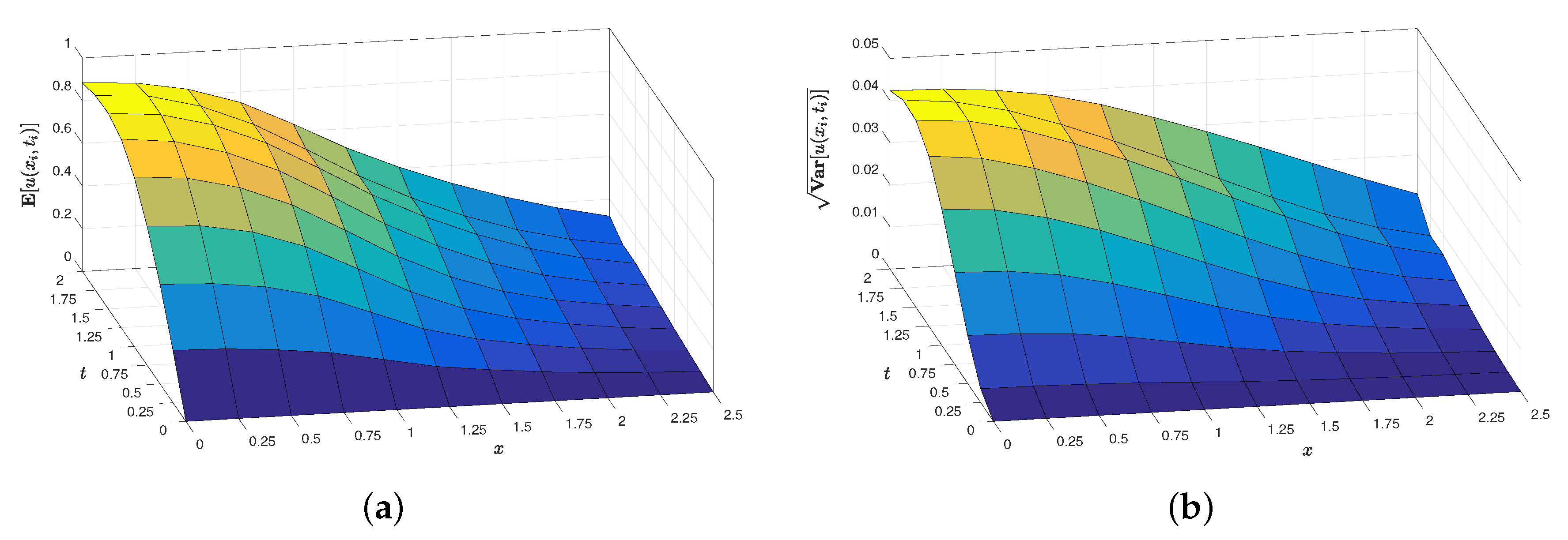
The exact computation of the expectation and the standard deviation of the solution s.p. in Equations (56) and (57), considering both a and b r.v.’s, is not available as an exact point of view. The use of numerical techniques to compute the expectation and the standard deviation of the integrals appearing in Equation (56) is required. Therefore, it is necessary to transform these random integrals into deterministic ones before applying numerical techniques. To carry out this task, firstly, for a fixed point $(x,t)$, we took $K=2\times {10}^5$ realizations of the independent r.v.’s a and b, then we computed numerically these K deterministic integrals and finally we obtained the mean and the standard deviation of these K values. Figure 1a,b shows the numerical values for the expectation and the standard deviation of the exact solution s.p. in Equations (56) and (57).

Figure 1. (a) Surface of the expectation $\mathbb{E}\left[u\right(x,t\left)\right]$; and (b) surface of the standard deviation $\sqrt{\mathrm{Var}\left[u\right(x,t\left)\right]}$. Both statistical moment functions correspond to the exact solution s.p. in Equations (56) and (57) of the random IVP in Equations (52)–(55) on the domain $(x,t)\in [0,2.5]\times [0,2]$ considering $a\sim N_{[0.9,1.1]}(1;0.05)$ and $b\sim {\mathrm{Beta}}_{[0.4,0.6]}(2;2)$.

Now, we obtain our approximation solution s.p. for the problem in Equations (52)–(55) as well as its expectation and standard deviation. Finally, we establish the corresponding comparisons between both statistical moment functions the approximate ones and the exact ones. By applying the random Fourier exponential transform to the problem in Equations (52)–(55) the random initial value transformed problem in Equations (30)–(33) is obtained with $c=1$, which can be expressed as the random linear system in Equation (34) with fixed $\xi \in \mathbb{R}$ and

$$L\left(\xi \right)=\left[\begin{array}{cc}0& 1\\ -(a+{\xi }^2)& -2b\end{array}\right],B\left(t\right)\left(\xi \right)=B\left(\xi \right)=\left[\begin{array}{c}0\\ \Phi \left(\xi \right)\end{array}\right]=\left[\begin{array}{c}0\\ \sqrt{\frac{2}{\pi }}\frac{sin\left(\xi \right)}{\xi }\end{array}\right],Y_0=Y_0\left(\xi \right)=\left[\begin{array}{c}0\\ e^{-\frac{{\xi }^2}{2}}\end{array}\right].$$

(58)

Random matrix $L\left(\xi \right)\in L_4^{2\times 2}(\Omega )$ because r.v.’s a and b are truncated r.v.’s. The condition in Equation (37) on the matrix $L\left(\xi \right)$, defined in Equation (58), is satisfied because the r.v.’s a and b are truncated ones, and furthermore $B\left(\xi \right)$ and $Y_0\left(\xi \right)$ are 4-absolutely integrables in $\mathbb{R}$. Note that $L\left(\xi \right)$ is a constant matrix with respect to t, then we can use Equation (15). Furthermore ,as $B\left(\xi \right)$ is also constant an explicit solution s.p. for the random linear system in Equation (34), Equation (58) is given by

$$\begin{array}{ccc}\hfill X\left(t\right)\left(\xi \right)=e^{L\left(\xi \right)t}\left\{Y_0+{\int }_0^t{e}^{-L\left(\xi \right)v}B\left(\xi \right)\mathrm{d}v\right\}& =& e^{L\left(\xi \right)t}\left\{Y_0+{\left[-L{\left(\xi \right)}^{-1}{e}^{-L\left(\xi \right)s}\right]}_{s=0}^{s=t}B\left(\xi \right)\right\}\hfill \\ & =& e^{L\left(\xi \right)t}\left\{Y_0+\left[-L{\left(\xi \right)}^{-1}\left(e^{-L\left(\xi \right)t}-I\right)\right]B\left(\xi \right)\right\}\hfill \\ & =& e^{L\left(\xi \right)t}\left(Y_0+L{\left(\xi \right)}^{-1}B\left(\xi \right)\right)-L{\left(\xi \right)}^{-1}B\left(\xi \right),\hfill \end{array}$$

(59)

being

$$L{\left(\xi \right)}^{-1}=\left[\begin{array}{cc}{\displaystyle \frac{-2b}{\alpha }}& -{\displaystyle \frac{1}{\alpha }}\\ 1& 0\end{array}\right],L{\left(\xi \right)}^{-1}B\left(\xi \right)=\left[\begin{array}{c}-{\displaystyle \frac{1}{\alpha }}\sqrt{{\displaystyle \frac{2}{\pi }}}{\displaystyle \frac{sin\left(\xi \right)}{\xi }}\\ 0\end{array}\right],\alpha =a+{\xi }^2.$$

(60)

and

$$e^{L\left(\xi \right)t}\mathrm{the}\mathrm{exponential}\mathrm{matrix}\mathrm{defined}\mathrm{in}\mathrm{Case}2,\mathrm{Equation}(),\mathrm{with}c=1,$$

(61)

because the parameter $\gamma =a-b^2>0$ and hence $b^2<a+{\xi }^2$, that is, $b^2<\alpha$.

Using Equations (59) and (60) and the introduced notation $[1,0]X\left(t\right)\left(\xi \right)=U\left(t\right)\left(\xi \right)$, the solution s.p. $U\left(t\right)\left(\xi \right)$ of the random initial value transformed problem in Equations (30)–(33) with $c=1$ is given by Equation (41) and takes the form

$$\begin{array}{c}U\left(t\right)\left(\xi \right)=\hfill \\ \hfill {\displaystyle \frac{e^{-bt}sin\left(t\sqrt{\alpha -b^2}\right)}{\sqrt{\alpha -b^2}}}{e}^{-\frac{{\xi }^2}{2}}+{\displaystyle \frac{1}{\alpha }}\sqrt{{\displaystyle \frac{2}{\pi }}}{\displaystyle \frac{sin\left(\xi \right)}{\xi }}\left(1-e^{-bt}\left(cos\left(t\sqrt{\alpha -b^2}\right)+{\displaystyle \frac{bsin\left(t\sqrt{\alpha -b^2}\right)}{\sqrt{\alpha -b^2}}}\right)\right),\end{array}$$

(62)

for $t>0$ and fixed $\xi \in \mathbb{R}$. Now, taking into account that $U\left(t\right)\left(\xi \right)=U\left(t\right)(-\xi )$ and lies in $\mathbb{R}$ for each $\xi \in \mathbb{R}$, the recovered solution s.p. $u(x,t)$ of the original random partial differential problem in Equations (52)–(55) given by Equation (42) takes the form

$$u(x,t)=\frac{1}{\sqrt{2\pi }}{\int }_{-\infty }^{+\infty }U\left(t\right)\left(\xi \right)cos\left(\xi x\right)\mathrm{d}\xi ,-\infty <x<+\infty ,t>0.$$

(63)

Using that $U\left(t\right)\left(\xi \right)$ is an even function in $\xi \in \mathbb{R}$ and denoting $U\left(t\right)\left(\xi \right)=X_1\left(t\right)\left(\xi \right)$, the  numerical values of the expectation in Equation (48) of the approximate solution s.p. of the problem in Equations (52)–(55) can be written as follows

$$\mathbb{E}\left[u_N^{\mathrm{G}-\mathrm{H}}(x,t)\right]=\frac{1}{\sqrt{2\pi }}\sum _{j=1}^N{\rho }_{j}cos\left({\xi }_{j}x\right)e^{{\xi }_j^2}\mathbb{E}\left[X_1\left(t\right)\left(\xi \right)\right],t>0,$$

(64)

where ${\rho }_j$, $j=1,\dots ,N$ are the weights of the Gauss–Hermite quadrature formula (see Equation (45)) and ${\xi }_j$ are the roots of the deterministic Hermite polynomial, $H_N$, of degree N. The approximate values of the standard deviation can be computed by

$$\sqrt{\mathrm{Var}\left[u_N^{\mathrm{G}-\mathrm{H}}(x,t)\right]}=\sqrt{\mathbb{E}\left[{\left(u_N^{\mathrm{G}-\mathrm{H}}(x,t)\right)}^2\right]-{\left(\mathbb{E}\left[u_N^{\mathrm{G}-\mathrm{H}}(x,t)\right]\right)}^2},$$

(65)

where

$$\mathbb{E}\left[{\left(u_N^{\mathrm{G}-\mathrm{H}}(x,t)\right)}^2\right]=\frac{1}{2\pi }\sum _{j=1}^N\sum _{\ell =1}^N{\rho }_j{\rho }_{\ell }cos\left({\xi }_{j}x\right)cos\left({\xi }_{\ell }x\right)e^{{\xi }_j^2+{\xi }_{\ell }^2}\mathbb{E}\left[X_1\left(t\right)\left({\xi }_j\right)X_1\left(t\right)\left({\xi }_{\ell }\right)\right],t>0.$$

(66)

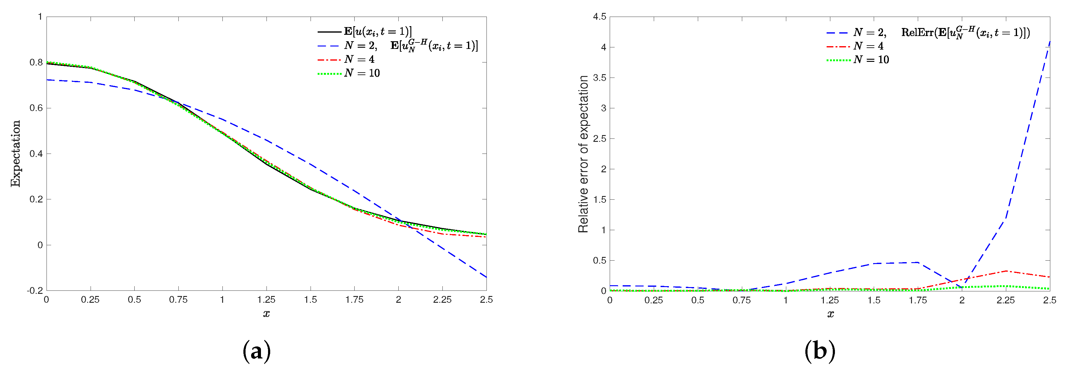
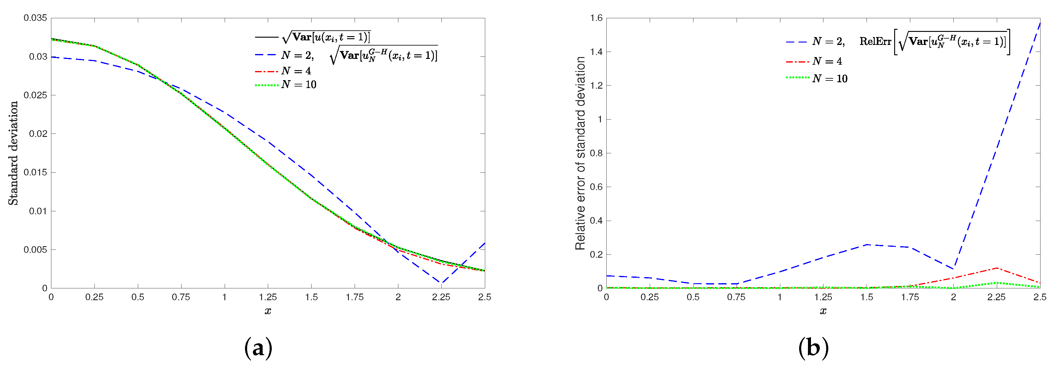
Figure 2 and Figure 3 show a comparative study of both the expectation and the standard deviation at $t=1$ on the spatial domain $x_i\in [0,2.5]$, $x_i=ih$, $0\le i\le 10$, $h=0.25$, for both the theoretical and the approximate solution s.p. of the random problem in Equations (52)–(55). Computation time of our method is competitive for the degrees N of the Hermite’s polynomial considered. For example, $2.34625$ s (CPU time spent in the Wolfram Language kernel) in total for computing both approximations the expectation $\mathbb{E}\left[u_N^{\mathrm{G}-\mathrm{H}}(x_i,1)\right]$ (Equation (64)), and the standard deviation $\sqrt{\mathrm{Var}\left[u_N^{\mathrm{G}-\mathrm{H}}(x_i,1)\right]}$ (Equations (64)–(66)) versus $20.2656$ s in total used in the calculation of the theoretical ones. The computation times are reduced for our method when the degree N of the Hermite’s polynomial decreases, for example, taking $N=6$ the time spent is $1.6567$ s.

Figure 2. (a) Expectation, $\mathbb{E}\left[u(x_i,1)\right]$, of the exact solution s.p. in Equations (56) and (57) vs. their corresponding numerical approximations, $\mathbb{E}\left[u_N^{\mathrm{G}-\mathrm{H}}(x_i,1)\right]$ (Equation (64)), by random Gauss–Hermite quadrature using Hermite’s polynomials of degree $N\in \{2,4,10\}$, at the time instant $t=1$ and on the spatial domain $0\le x\le 2.5$. (b) Relative errors of the expectation, $\mathrm{RelErr}\left[{\mathbb{E}}_N^{\mathrm{G}-\mathrm{H}}(x_i,1)\right]$ (Equation (67)) when it is considered Hermite’s polynomials of degree $N\in \{2,4,10\}$ and the spatial domain $0\le x\le 2.5$.

Figure 3. (a) Standard deviation, $\sqrt{\mathrm{Var}\left[u(x_i,1)\right]}$, of the exact solution s.p. in Equations (56) and (57) vs. their corresponding numerical approximations, $\sqrt{\mathrm{Var}\left[u_N^{\mathrm{G}-\mathrm{H}}(x_i,1)\right]}$ (Equations (64)–(66)), by random Gauss–Hermite quadrature using Hermite’s polynomials of degree $N\in \{2,4,10\}$, at the time instant $t=1$ and on the spatial domain $0\le x\le 2.5$. (b) Relative errors of the standard deviation, $\mathrm{RelErr}\left[\sqrt{{\mathrm{Var}}_N^{\mathrm{G}-\mathrm{H}}(x_i,1)}\right]$ (Equation (68)) when it is considered Hermite’s polynomials of degree $N\in \{2,4,10\}$ and the spatial domain $0\le x\le 2.5$.

In Figure 2a and Figure 3a, we plot at $t=1$ the expectation, $\mathbb{E}\left[u(x_i,1)\right]$, and the standard deviation, $\sqrt{\mathrm{Var}\left[u(x_i,1)\right]}$, respectively, of the exact solution s.p. in Equations (56) and (57) vs. the respective approximate ones, $\mathbb{E}\left[u_N^{\mathrm{G}-\mathrm{H}}(x_i,1)\right]$ (Equation (64)), and $\sqrt{\mathrm{Var}\left[u_N^{\mathrm{G}-\mathrm{H}}(x_i,1)\right]}$ (Equations (64)–(66)), for different degrees N of the Hermite polynomials: $N=\{2,4,10\}$. In Figure 2b and Figure 3b, it is observed that the approximations improve as the degree N increases because the relative errors computed using the following expressions decrease

$$\begin{array}{ccc}\hfill \mathrm{RelErr}\left(\mathbb{E}\left[u_N^{\mathrm{G}-\mathrm{H}}(x,t)\right]\right)& =& \left|\frac{\mathbb{E}\left[u(x,t)\right]-\mathbb{E}\left[u_N^{\mathrm{G}-\mathrm{H}}(x,t)\right]}{\mathbb{E}\left[u\right(x,t\left)\right]}\right|,\hfill \end{array}$$

(67)

$$\begin{array}{ccc}\hfill \mathrm{RelErr}\left(\sqrt{\mathrm{Var}\left[u_N^{\mathrm{G}-\mathrm{H}}(x,t)\right]}\right)& =& \left|\frac{\sqrt{\mathrm{Var}\left[u\right(x,t\left)\right]}-\sqrt{\mathrm{Var}\left[u_N^{\mathrm{G}-\mathrm{H}}(x,t)\right]}}{\sqrt{\mathrm{Var}\left[u\right(x,t\left)\right]}}\right|.\hfill \end{array}$$

(68)

An interesting quantitative study of global errors, in the spatial domain $[0,2.5]$ for a fixed time t and a number n of spatial points $x_i$, $0\le i\le n$, was also carried out considering the root mean squared errors (RMSEs):

$$\begin{array}{ccc}\hfill \mathrm{RMSE}\left[\mathbb{E}(x_i,t)\right]& =& \sqrt{\frac{1}{(n+1)}{\sum }_{i=0}^n{\left(\mathbb{E}\left[u(x_i,t)\right]-\mathbb{E}\left[u_N^{\mathrm{G}-\mathrm{H}}(x_i,t)\right]\right)}^2},\hfill \end{array}$$

(69)

$$\begin{array}{ccc}\hfill \mathrm{RMSE}\left[\sqrt{\mathrm{Var}(x_i,t)}\right]& =& \sqrt{\frac{1}{(n+1)}{\sum }_{i=0}^n{\left(\sqrt{\mathrm{Var}\left[u(x_i,t)\right]}-\sqrt{\mathrm{Var}\left[u_N^{\mathrm{G}-\mathrm{H}}(x_i,t)\right]}\right)}^2},\hfill \end{array}$$

(70)

Table 4 collects the results obtained and shows that the proposed method provides good approximations to the numerical values of the expectation and the standard deviation of the exact solution s.p. in Equations (56) and (57). We observe that it is sufficient to consider a Hermite’s polynomial of degree $N=6$, in order to obtain reasonable approximations to the exact ones.

Table 4. Values of the RMSEs for the expectation, $\mathrm{RMSE}\left[\mathbb{E}(x_i,t)\right]$ (Equation (69)) and the standard deviation $\mathrm{RMSE}\left[\sqrt{\mathrm{Var}(x_i,t)}\right]$ (Equation (70)), at the time instant $t=1$ along the spatial domain $[0,2.5]$ considering the set of points $x_i=ih$, $0\le i\le n=10$, with the stepsize $h=0.25$.

N	$\mathbf{RMSE}\left[\mathbb{E}({\mathit{x}}_{\mathit{i}},1)\right]$	$\mathbf{RMSE}\left[\sqrt{\mathbf{Var}({\mathit{x}}_{\mathit{i}},1)}\right]$
2	$8.8178e-02$	$2.2916e-03$
4	$1.1892e-02$	$1.7732e-04$
6	$9.0351e-03$	$1.4160e-04$
8	$8.9287e-03$	$1.1546e-04$
10	$6.0334e-03$	$6.4509e-05$

Note that in this example the errors due to the calculus of an approximate solution s.p. of the auxiliary system in Equations (34) and (58) do not appear in the errors computed because this solution, $U\left(t\right)\left(\xi \right)$, was calculated in an exact way (see Equation (62)). Then, the relative errors plotted in Figure 2b and Figure 3b and the RMSEs collect in Table 4 include mainly the errors due to the random Gauss–Hermite quadrature formula of degree N.

Algorithm 1 summarizes the steps to compute the approximations of the expectation and the standard deviation of the solution s.p. in Equation (47).

Algorithm 1 Calculation procedure for the expectation and the standard deviation of the approximated solution s.p. $u_N^{\mathrm{G}-\mathrm{H}}(x,t)$ (Equation (47)) of the problem in Equations (1)–(3).

Require:  Guarantee that the random input data of problem in Equations (1)–(3): a, b and c are r.v.’s in $L_4(\Omega )$ and $\varphi (x,t)$, $f_1\left(x\right)$ and $f_2\left(x\right)$ are m.f. continuous s.p.’s with a finite degree of randomness and m.f. absolutely integrable with respect to the spatial variable in the real line. Additionally, the s.p. $\varphi (x,t)$ can be chosen with at most a finite number of jump discontinuities in the variable x.   1: Fix a point $(x,t)$, $x\in \mathbb{R}$, $t>0$.  2: Choose the degree N of the Hermite polynomial, $H_N(·)$, and compute $H_{N-1}(·)$ and $H_N(·)$.  3: for$j=1$ to N do 4:   Compute the j roots, ${\theta }_j$, of $H_N(·)$;  5: end for  6: for$j=1$ to N do 7:   Compute the weights, ${\rho }_j$, of $H_N(·)$ using Equation (45).  8: end for  9: Construct the random matrix $L\left({\theta }_j\right)$ using Equation (35) where $\xi$ represent a particular ${\theta }_j$.  10: if the entries of random matrix $L\left({\theta }_j\right)$ verifies the condition in Equation (37) then 11:   continue to the following step  12: else 13:   change the election of the r.v.’s a, b and c and check again the condition in Equation (37).  14: end if  15: Compute the random Fourier exponential transforms of the input data $\varphi (x,t)$, $f_1\left(x\right)$ and $f_2\left(x\right)$.  16: Construct the random vector s.p. $B\left(x\right)\left({\theta }_j\right)$ and the random vector $Y_0\left({\theta }_j\right)$ using Equation (36).  17: for$j=1$ to N do 18:   Compute numerically the expectation of the j-solutions s.p.’s, $X_1\left(t\right)\left({\theta }_j\right)=[1,0]X\left(t\right)\left({\theta }_j\right)$, of the random linear system in Equations (34)–(36) using Equation (41) and the adequate case in Equations (38)–(40) for the exponential matrix of $L\left({\theta }_j\right)t$. These j expectations are denoted by $\mathbb{E}\left[X_1\left(t\right)\left({\theta }_j\right)\right]$.  19: end for  20: Compute the expectation, $\mathbb{E}\left[u_N^{\mathrm{G}-\mathrm{H}}(x,t)\right]$, and the standard deviation, $\sqrt{\mathrm{Var}\left[u_N^{\mathrm{G}-\mathrm{H}}(x,t)\right]}$, of the approximated solution s.p. $u_N^{\mathrm{G}-\mathrm{H}}(x,t)$ (Equation (47)) using the explicit expressions in Equations (48), (49) and (50).

4. Gauss–Laguerre Solution of a Random Heterogeneous Telegraph Model

This section is addressed to construct random Gauss–Laguerre quadrature formulae for the numerical solution of the model in Equations (4)–(7). Although the approach is similar to the one developed in Section 3, here we use the random Fourier sine transform acting on the temporal variable. The random variable coefficient transformed problem requires a numerical approach that is constructed in two stages. Firstly, the Gauss–Laguerre quadrature of the random inverse Fourier sine transform and further Monte Carlo simulations at appropriated root points of the Laguerre polynomials.

Let $V\left(x\right)\left(\xi \right)={\mathfrak{F}}_s\left[u(x,·)\right]\left(\xi \right)$ be the Fourier sine transform of the unknown $u(x,·)$:

$$V\left(x\right)\left(\xi \right)={\mathfrak{F}}_s\left[u(x,·)\right]\left(\xi \right)={\int }_0^{+\infty }u(x,t)sin\left(\xi t\right)\mathrm{dt},\xi >0,x>0.$$

(71)

From Theorem 1 of [16], we have

$${\mathfrak{F}}_s\left[h^{\prime \prime }\left(t\right)\right]\left(\xi \right)=\xi h\left(0\right)-{\xi }^2{\mathfrak{F}}_s\left[h\left(t\right)\right]\left(\xi \right),\xi >0.$$

(72)

Let us denote

$$\begin{array}{ccc}\hfill G_1\left(\xi \right)& =& {\mathfrak{F}}_s\left[u(0,·)\right]\left(\xi \right)={\mathfrak{F}}_s\left[g_1\left(t\right)\right]\left(\xi \right),\xi >0,\hfill \end{array}$$

(73)

$$\begin{array}{ccc}\hfill G_2\left(\xi \right)& =& {\mathfrak{F}}_s\left[u_x(0,·)\right]\left(\xi \right)={\mathfrak{F}}_s\left[g_2\left(t\right)\right]\left(\xi \right),\xi >0,\hfill \end{array}$$

(74)

$$\begin{array}{ccc}\hfill \Psi \left(x\right)\left(\xi \right)& =& {\mathfrak{F}}_s\left[\psi (x,·)\right]\left(\xi \right),x>0,\xi >0.\hfill \end{array}$$

(75)

Let us assume that the s.p.’s $k\left(x\right)$, $a\left(x\right)$, $\psi (x,t)$, $g_1\left(t\right)$, $g_2\left(t\right)$ and $g\left(x\right)$ of the problem in Equations (4)–(7) are m.f. continuous with a finite degree of randomness. Let $k\left(x\right)$ be a positive s.p. 4-differentiable and let $\psi (x,t)$, $g_1\left(t\right)$, $g_2\left(t\right)$ be m.f. absolutely integrable s.p.’s in $t>0$, that is,

$${\int }_0^{+\infty }{\parallel \psi (x,t)\parallel }_4\mathrm{d}t<+\infty (x>0\mathrm{fixed}),{\int }_0^{+\infty }\parallel g_1{\left(t\right)\parallel }_4\mathrm{d}t<+\infty ,{\int }_0^{+\infty }{\parallel g_2\left(t\right)\parallel }_4\mathrm{d}t<+\infty .$$

By applying random Fourier sine transform to the problem in Equations (4)–(7) and using Equations (72)–(74), one gets

$$\xi g\left(x\right)-{\xi }^{2}V\left(x\right)\left(\xi \right)=\frac{d}{dx}\left(k\left(x\right)\frac{d}{dx}\left(V\left(x\right)\right)\left(\xi \right)\right)+a\left(x\right)V\left(x\right)\left(\xi \right)+\Psi \left(x\right),$$

(76)

or

$$\frac{d^2}{d{x}^2}\left(V\left(x\right)\right)\left(\xi \right)+\frac{k^{\prime }\left(x\right)}{k\left(x\right)}\frac{d}{dx}\left(V\left(x\right)\right)\left(\xi \right)+\frac{a\left(x\right)+{\xi }^2}{k\left(x\right)}V\left(x\right)\left(\xi \right)=\frac{\Psi \left(x\right)\left(\xi \right)-\xi g\left(x\right)}{k\left(x\right)},\xi >0\mathrm{fixed},$$

(77)

together with

$$\begin{array}{c}\hfill \begin{array}{c}V\left(0\right)\left(\xi \right)=G_1\left(\xi \right),\hfill \\ {\displaystyle \frac{d}{dx}}\left(V\left(0\right)\right)\left(\xi \right)=G_2\left(\xi \right).\hfill \end{array}\end{array}$$

(78)

The solution to the problem in Equations (77) and (78) is the first component of the solution of extended random linear differential system, $V\left(x\right)\left(\xi \right)=[1,0]X\left(x\right)\left(\xi \right)$,

$$\begin{array}{c}\hfill \left.\begin{array}{ccc}\hfill X^{\prime }\left(x\right)\left(\xi \right)& =& L\left(x\right)\left(\xi \right)X\left(x\right)\left(\xi \right)+B\left(x\right)\left(\xi \right),x>0,\hfill \\ \hfill X\left(0\right)\left(\xi \right)& =& Y_0\left(\xi \right),\hfill \end{array}\right\}\end{array}$$

(79)

where

$$\begin{array}{c}\hfill L\left(x\right)\left(\xi \right)=\left[\begin{array}{cc}0& 1\\ -{\displaystyle \frac{{\xi }^2+a\left(x\right)}{k\left(x\right)}}& -{\displaystyle \frac{k^{\prime }\left(x\right)}{k\left(x\right)}}\end{array}\right],B\left(x\right)\left(\xi \right)=\left[\begin{array}{c}0\\ {\displaystyle \frac{\Psi \left(x\right)\left(\xi \right)-\xi g\left(x\right)}{k\left(x\right)}}\end{array}\right],Y_0\left(\xi \right)=\left[\begin{array}{c}{G}_1\left(\xi \right)\\ G_2\left(\xi \right)\end{array}\right].\end{array}$$

(80)

By Section 2, assuming that 4-s.p.’s $a\left(x\right)$, $k\left(x\right)$ and $k^{\prime }\left(x\right)$ satisfy the moment condition in Equation (12) for every $x>0$, it is guaranteed that the entries of the matrix s.p. $L\left(x\right)\left(\xi \right)={\left({\ell }_{i,j}\left(x\right)\right)}_{2\times 2}\in L_4^{2\times 2}(\Omega )$, for $\xi >0$ fixed, and satisfy the condition in Equation (12). Furthermore, the condition in Equation (12) guarantees that $L\left(x\right)\left(\xi \right)$ is 4-locally absolutely integrable in $x\in [0,x_1]$:

$${\int }_0^{x_1}{\parallel {\ell }_{i,j}\left(x\right)\parallel }_4\mathrm{d}x={\int }_0^{x_1}{\left(\mathbb{E}\left[\right|{\ell }_{i,j}\left(x\right){|}^4]\right)}^{1/4}\mathrm{d}x\le {\int }_0^{x_1}{\left(m_{i,j}{\left(h_{i,j}\right)}^4\right)}^{1/4}\mathrm{d}x={\left(m_{i,j}\right)}^{1/4}{h}_{i,j}{x}_1<+\infty .$$

Furthermore, it is verified that vector s.p.’s both $B\left(x\right)\left(\xi \right)$ and $Y_0\left(x\right)\left(\xi \right)$ lie in $L_4^{2\times 1}(\Omega )$ and they are absolutely integrables in $x\in [0,+\infty )$.

Note that, unlike the case of Section 3, here the system in Equations (79) and (80) does not have an explicit solution s.p. because, in Equation (14), the random fundamental matrix ${\Phi }_L(x;0)$ is unknown and thus one needs a numerical approach. By using random inverse Fourier sine transform to $V\left(x\right)\left(\xi \right)$, one gets

$$u(x,t)=\frac{2}{\pi }{\int }_0^{\infty }V\left(x\right)\left(\xi \right)sin\left(\xi t\right)\mathrm{d}\xi =\frac{2}{\pi }{\int }_0^{\infty }[1,0]X\left(x\right)\left(\xi \right)sin\left(\xi t\right)\mathrm{d}\xi =\frac{2}{\pi }{\int }_0^{\infty }{X}_1\left(x\right)\left(\xi \right)sin\left(\xi t\right)\mathrm{d}\xi ,$$

(81)

where $X_1\left(x\right)\left(\xi \right)=[1,0]X\left(x\right)\left(\xi \right).$ Now, we apply random Gauss–Laguerre quadrature to approximate the integral of Equation (81). For s.p. $\mathcal{J}\left(\xi \right)\in L_2(\Omega )$ being m.f.-absolutely integrable with respect to $\xi >0$, let us consider the following integral

$$I=I\left[\mathcal{J}\right]={\int }_0^{\infty }\mathcal{J}\left(\xi \right)e^{-\xi }\mathrm{d}\xi ,\xi >0,$$

(82)

which is a r.v. Since $0<e^{-\xi }\le 1$ for all $\xi >0$ and s.p. $\mathcal{J}\left(\xi \right)\in L_2(\Omega )$ being m.f.-absolutely integrable respect to $\xi >0$ one gets

$${\parallel I\parallel }_2={∥{\int }_0^{+\infty }\mathcal{J}\left(\xi \right)e^{-\xi }\mathrm{d}\xi ∥}_2\le {\int }_0^{+\infty }{∥\mathcal{J}\left(\xi \right)e^{-\xi }∥}_2\mathrm{d}\xi \le {\int }_0^{+\infty }{∥\mathcal{J}\left(\xi \right)∥}_2\mathrm{d}\xi <+\infty .$$

Then, $I=I\left[\mathcal{J}\right]$ is well-defined. Assuming that $\mathcal{J}\left(\xi \right)\in L_2(\Omega )$ has continuous sample trajectories, i.e., $\mathcal{J}\left(\xi \right)\left(\omega \right)$ is continuous with respect to $\xi >0$ for all $\omega \in \Omega$, then r.v. in Equation (82) coincides, with probability 1, with the (deterministic) sample integrals

$$I\left(\omega \right)=I\left[\mathcal{J}\right]\left(\omega \right)={\int }_0^{+\infty }\mathcal{J}(\xi ;\omega )e^{-\xi }\mathrm{d}\xi ,\omega \in \Omega ,$$

which are well-defined and thus they are convergent for all $\omega \in \Omega$ (see Appendix I of [13]). Then, taking advantage of the Gauss–Laguerre quadrature formula of degree N, see page 890 of [19], we can consider the following numerical approximation for each event $\omega \in \Omega$

$$I_N^{\mathrm{G}-\mathrm{L}}\left[\mathcal{J}\right]\left(\omega \right)=\sum _{j=1}^N{\nu }_j\mathcal{J}({\vartheta }_j;\omega ),{\nu }_j=\frac{{\vartheta }_j}{{\left[(N+1)L_{N+1}\left({\vartheta }_j\right)\right]}^2},$$

(83)

where ${\vartheta }_j$ is the jth root of the deterministic Laguerre polynomial, $L_N\left(\vartheta \right)$, of degree N and ${\nu }_j$ is the weight. This quadrature formula to approximate a random integral of the type in Equation (82) is applied to the r.v. $u(x,t)$ given by Equation (81) taking

$$\mathcal{J}\left(\xi \right)=\mathcal{J}(x,t,\xi )=\frac{2}{\pi }{X}_1\left(x\right)\left(\xi \right)sin\left(\xi t\right)e^{\xi }.$$

Given the degree N, let us denote by $u_N^{\mathrm{G}-\mathrm{L}}(x,t)$ the Gauss–Laguerre s.p. approximation of degree N of the exact solution s.p. $u(x,t)$ of the random problem in Equations (4)–(7), evaluated at $(x,t)$ and expressed as the r.v.

$$u_N^{\mathrm{G}-\mathrm{L}}(x,t)=\frac{2}{\pi }\sum _{j=1}^N{\nu }_{j}sin\left({\vartheta }_{j}t\right)e^{{\vartheta }_j}{X}_1\left(x\right)\left({\vartheta }_j\right).$$

(84)

Note that, unlike to the problem of Section 3, the exact solution $X_1\left(x\right)\left({\vartheta }_j\right)$ is obtained using Monte Carlo simulation because it is not available. That is, the evaluation of the solution s.p. of the random linear system in Equation (79) at ${\vartheta }_j$ is not available in an explicit form, thus the expectation is approximated using Monte Carlo approach, as treated in Section 2, and denoted by ${\mathbb{E}}_{MC}^K\left[{\overline{X}}_1\left(x\right)\left({\vartheta }_j\right)\right]$ where K represents the number of realizations used in the Monte Carlo simulation and ${\overline{X}}_1\left(x\right)\left({\vartheta }_j\right)$ the deterministic numerical solution obtained after taking K realizations. Thus, the final expression for the approximation of the $\mathbb{E}\left[u\right(x,t\left)\right]$ takes the form

$$\mathbb{E}\left[u_N^{\mathrm{G}-\mathrm{L}}(x,t)\right]\approx \mathbb{E}\left[u_{N,K}^{\mathrm{G}-\mathrm{L}}(x,t)\right]=\frac{2}{\pi }\sum _{j=1}^N{\nu }_{j}sin\left({\vartheta }_{j}t\right)e^{{\vartheta }_j}{\mathbb{E}}_{MC}^K\left[{\overline{X}}_1\left(x\right)\left({\vartheta }_j\right)\right],x>0,t>0.$$

(85)

The standard deviation of the approximate solution s.p. $u_N^{\mathrm{G}-\mathrm{L}}(x,t)$ (Equation (84)), can be computed taking the square root of the following expression

$$\begin{array}{c}\mathrm{Var}\left[u_N^{\mathrm{G}-\mathrm{L}}(x,t)\right]\approx \mathrm{Var}\left[u_{N,K}^{\mathrm{G}-\mathrm{L}}(x,t)\right]=\hfill \\ {\left(\frac{2}{\pi }\right)}^2\sum _{j=1}^N\sum _{\ell =1}^N{\nu }_j{\nu }_{\ell }sin\left({\vartheta }_{j}t\right)sin\left({\vartheta }_{\ell }t\right)e^{{\vartheta }_j+{\vartheta }_{\ell }}\left({\mathbb{E}}_{MC}^K\left[{\overline{X}}_1\left(x\right)\left({\vartheta }_j\right){\overline{X}}_1\left(x\right)\left({\vartheta }_{\ell }\right)\right]\right.\\ \left.-{\mathbb{E}}_{MC}^K\left[{\overline{X}}_1\left(t\right)\left({\vartheta }_j\right)\right]{\mathbb{E}}_{MC}^K\left[{\overline{X}}_1\left(t\right)\left({\vartheta }_{\ell }\right)\right]\right)\\ \hfill ={\left(\frac{2}{\pi }\right)}^2\sum _{j=1}^N\sum _{\ell =1}^N{\nu }_j{\nu }_{\ell }sin\left({\vartheta }_{j}t\right)sin\left({\vartheta }_{\ell }t\right)e^{{\vartheta }_j+{\vartheta }_{\ell }}{\mathrm{Cov}}_{MC}^K\left[{\overline{X}}_1\left(x\right)\left({\vartheta }_j\right),{\overline{X}}_1\left(x\right)\left({\vartheta }_{\ell }\right)\right].\end{array}$$

(86)

A Numerical Example

Consider the random heterogeneous telegraph type problem in Equation (4)–(7) with the following input data

$$\begin{array}{cc}\hfill \left.\begin{array}{c}k\left(x\right)=1+bcos\left(\pi x\right),a\left(x\right)=e^{-ax},\psi (x,t)=e^{-(x+t)}\hfill \\ g_1\left(t\right)=0,g_2\left(t\right)=0,g\left(x\right)=0\hfill \end{array}\right\},& x>0,t>0,\end{array}$$

(87)

where parameters a and b are assumed to be independent r.v.’s; specifically, a has a uniform distribution giving values in $[0,1]$, that is, $a\sim Un(0,1)$, and $b>0$ has an exponential distribution of parameter 2 truncated on the interval $[0.1,0.2]$, that is, $b\sim Ex{p}_{[0.1,0.2]}\left(2\right)$. Then, it is verified that s.p.’s $k\left(x\right)$ and $a\left(x\right)$ and functions $\psi (x,t)$, $g_1\left(t\right)$, $g_2\left(t\right)$ and $g\left(x\right)$ are 4-continuous and 4-absolutely integrable with respect to the time variable those depending on t. Furthermore, $k\left(x\right)$ is positive and 4-differentiable. Note that s.p.’s $k\left(x\right)$ and $a\left(x\right)$ depend on a single r.v., that is, they have a finite degree of randomness.

In this example, the elements of the auxiliary random linear differential system in Equations (79) and (80) take the form

$$\begin{array}{c}\hfill L\left(x\right)\left(\xi \right)=\left[\begin{array}{cc}0& 1\\ -{\displaystyle \frac{{\xi }^2+e^{-ax}}{1+bcos\left(\pi x\right)}}& {\displaystyle \frac{b\pi sin\left(\pi x\right)}{1+bcos\left(\pi x\right)}}\end{array}\right],\\ \hfill B\left(x\right)\left(\xi \right)=\left[\begin{array}{c}0\\ {\displaystyle \frac{e^{-x}\xi }{(1+{\xi }^2)(1+bcos\left(\pi x\right))}}\end{array}\right],Y_0\left(\xi \right)=\left[\begin{array}{c}0\\ 0\end{array}\right],\end{array}$$

(88)

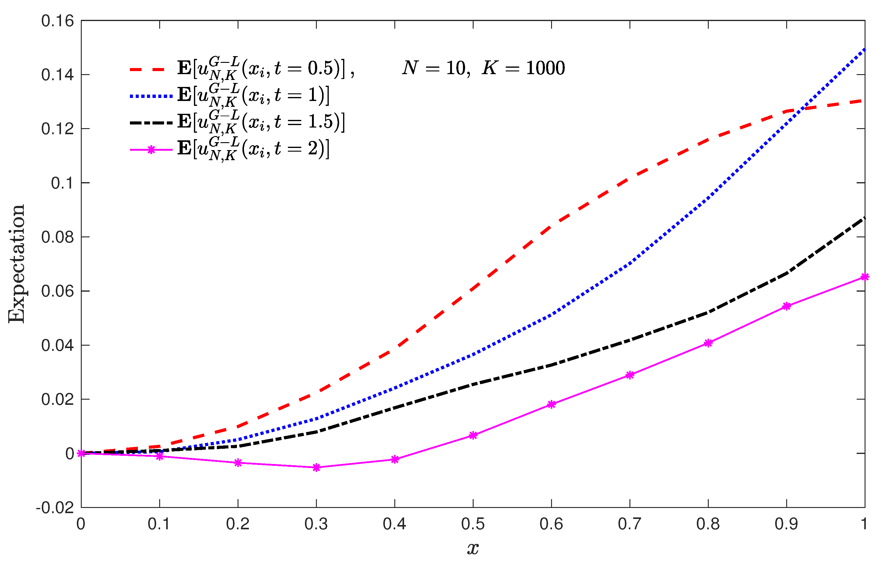
where in $B\left(x\right)\left(\xi \right)$ it is obtained that $\Psi \left(x\right)\left(\xi \right)={\mathfrak{F}}_s\left[\psi (x,t)\right]\left(\xi \right)=e^{-x}{\displaystyle \frac{\xi }{1+{\xi }^2}}$, $x>0$ for a fixed $\xi >0$. Observe that the entries of the matrix s.p. $L\left(x\right)\left(\xi \right)$ given in Equation (88) satisfies the moment condition in Equation (12) for every x because r.v.’s a and b are bounded. The random linear differential system in Equations (79) and (88) does not have an explicit solution s.p., thus we proceed as shown in Example 1 searching alternative approximations of Equations (79) and (88) via Monte Carlo simulations. Taking a particular number of realizations, K, over the r.v.’s a and b, we solve the K deterministic systems corresponding to Equations (79) and (88) for each ${\xi }_j$, $j=1,\cdots ,N$. The integer N represents the roots of the Laguerre polynomial of degree N and it must be fixed befor the computation of the K deterministic systems. We computed, for each ${\xi }_j$, the mean of the K solutions obtained, that is, ${\mathbb{E}}_{MC}^K\left[{\overline{X}}_1\left(x\right)\left({\xi }_j\right)\right]$, $j=1,\cdots ,N$. Finally, we can provide an approximation of the first and the second moments of the solution s.p. of the original problem in Equations (4)–(7) and (87) using the explicit expressions in Equations (85) and (86) where ${\vartheta }_j$ represents the jth root ${\xi }_j$, $j=1,\cdots ,N$. Algorithm 2 summarizes the procedure described above to compute the approximations of the expectation and the standard deviation of the solution s.p. in Equation (84). Figure 4 shows simulations of the expectation of the solution s.p. in Equation (84) at time instants $t=\{0.5,1,1.5,2\}$ on the spatial domain $0\le x\le 1$ considering the set of points $x_i=ih$, $0\le i\le n=10$, with the stepsize $h=0.1$. To carry out these simulations, $K=1000$ realizations for Monte Carlo method and $N=10$ for the Gauss–Laguerre quadrature were considered.

Figure 4. Simulations of the evolution along the time instants $t=0.5$, $t=1$, $t=1.5$ and $t=2$ of the approximated expectation, $\mathbb{E}\left[u_{N,K}^{\mathrm{G}-\mathrm{L}}(x_i,t)\right]$ (Equation (85)), of the solution s.p. $u_N^{\mathrm{G}-\mathrm{L}}(x,t)$ (Equation (84)) on the spatial domain $0\le x\le 1$ for $K=1000$ realizations via Monte Carlo and $N=10$ the degree of the Laguerre polynomial.

Now, to study the numerical convergence of the approximations of both the expectation and the standard deviation, we studied the behavior of their root mean square deviations (RMSD) in two stages: firstly, varying the number K of realizations in the Monte Carlo method but considering fixed the N in the Gauss–Laguerre quadrature; and, secondly, varying N but considering the number of realizations K fixed. For the first stage, Table 5 collects the RMSDs computed using the following notation

$$\begin{array}{ccc}\hfill \mathrm{RMSD}\left[\mathbb{E}\left[u_{N,K_{\ell }{K}_{\ell +1}}^{\mathrm{G}-\mathrm{L}}(x_i,t)\right]\right]& =& \sqrt{\frac{1}{(n+1)}{\sum }_{\ell =0}^n{\left(\mathbb{E}\left[u_{N,K_{\ell +1}}^{\mathrm{G}-\mathrm{L}}(x_i,t)\right]-\mathbb{E}\left[u_{N,K_{\ell }}^{\mathrm{G}-\mathrm{L}}(x_i,t)\right]\right)}^2},\hfill \end{array}$$

(89)

$$\begin{array}{ccc}\hfill \mathrm{RMSD}\left[\sqrt{\mathrm{Var}[u_{N,K_{\ell }{K}_{\ell +1}}^{\mathrm{G}-\mathrm{L}}(x_i,t)}]\right]& =& \sqrt{\frac{1}{(n+1)}{\sum }_{\ell =0}^n{\left(\sqrt{\mathrm{Var}[u_{N,K_{\ell +1}}^{\mathrm{G}-\mathrm{L}}(x_i,t)}-\sqrt{\mathrm{Var}[u_{N,K_{\ell }}^{\mathrm{G}-\mathrm{L}}(x_i,t)}\right)}^2},\hfill \end{array}$$

(90)

at time instant $t=1$ along the spatial domain $[0,1]$ considering the set of points $x_i=ih$, $0\le i\le n=10$, with the stepsize $h=0.1$. The integers $K_{\ell }$ and $K_{\ell +1}$ denote the realizations taken using Monte Carlo method to solve numerically the random linear differential system in Equations (79) and (88). The simulations $K_{\ell }$, $\ell =0,\cdots ,5$, correspond to $K_0=2500$, $K_1=5000$, $K_2={10}^4$, $K_3=2\times {10}^4$, $K_4=4\times {10}^4$ and $K_5=5\times {10}^4$ and $N=6$ is the degree fixed for the Laguerre polynomials. The decreasing trend of the RMSDs when compared to the previous realization is observed. A similar behavior can be observed when other degrees N are considered.

Table 5. Values of the RMSDs for the approximations of the expectation, $\mathrm{RMSD}\left[{\mathbb{E}}_{N,K_{\ell }{K}_{\ell +1}}^{\mathrm{G}-\mathrm{L}}(x_i,t)\right]$ (Equation (89)), and the standard deviation, $\mathrm{RMSD}\left[\sqrt{{\mathrm{Var}}_{N,K_{\ell }{K}_{\ell +1}}^{\mathrm{G}-\mathrm{L}}(x_i,t)}\right]$ (Equation (90)), at $t=1$ on the spatial domain $0\le x\le 1$, $N=6$ the degree of the Laguerre polynomial and the realizations $K_0=2500$, $K_1=5000$, $K_2={10}^4$, $K_3=2\times {10}^4$, $K_4=4\times {10}^4$ and $K_5=5\times {10}^4$.

${\mathit{K}}_{\mathit{\ell }}{\mathit{K}}_{\mathit{\ell }+1}$	$\mathbf{RMSD}\left[\mathbb{E}\left[{\mathit{u}}_{6,{\mathit{K}}_{\mathit{\ell }}{\mathit{K}}_{\mathit{\ell }+1}}^{\mathbf{G}-\mathbf{L}}({\mathit{x}}_{\mathit{i}},1)\right]\right]$	$\mathbf{RMSD}\left[\sqrt{\mathbf{Var}[{\mathit{u}}_{6,{\mathit{K}}_{\mathit{\ell }}{\mathit{K}}_{\mathit{\ell }+1}}^{\mathbf{G}-\mathbf{L}}({\mathit{x}}_{\mathit{i}},1)}]\right]$
$K_0{K}_1$	$2.81922e-05$	$2.91484e-05$
$K_1{K}_2$	$1.96565e-05$	$1.18180e-05$
$K_2{K}_3$	$1.11618e-05$	$2.49163e-06$
$K_3{K}_4$	$1.07918e-05$	$4.96128e-06$
$K_4{K}_5$	$3.59937e-06$	$2.83452e-06$

Algorithm 2 Calculation procedure for the expectation and the standard deviation of the approximated solution s.p. $u_N^{\mathrm{G}-\mathrm{L}}(x,t)$ (Equation (84)) of the problem in Equations (4)–(7).

Require:  Guarantee that the random input data $k\left(x\right)$, $a\left(x\right)$, $\psi (x,t)$, $g_1\left(t\right)$, $g_2\left(t\right)$ and $g\left(x\right)$ of problem in Equations (4)–(7) are m.f. continuous s.p.’s with a finite degree of randomness, and m.f. absolutely integrable s.p.’s with respect to the time variable those depending on t. Furthermore, $k\left(x\right)$ must be positive and 4-differentiable.  1: Fix a point $(x,t)$, $x>0$, $t>0$.   2: Choose the degree N of the Laguerre polynomial, $L_N(·)$, and compute $L_N(·)$ and $L_{N+1}(·)$.  3: for$j=1$ to N do 4:   Compute the j roots, ${\vartheta }_j$, of $L_N(·)$;  5: end for  6: for$j=1$ to N do 7:   Compute the weights, ${\nu }_j$, of $L_N(·)$ using Equation (83).   8: end for  9: Choose and carry out a number K of the realizations over the r.v.’s involve in the s.p.’s of the input data: $k\left(x\right)$, $a\left(x\right)$, $\psi (x,t)$, $g_1\left(t\right)$, $g_2\left(t\right)$ and $g\left(x\right)$.  10: Construct the matrix s.p. $L\left(x\right)\left({\vartheta }_j\right)$ given by Equation (80) where $\xi$ represent a particular ${\vartheta }_j$.  11: if the entries of matrix s.p. $L\left(x\right)\left({\vartheta }_j\right)$ verifies the condition in Equation (12) then 12:   continue to the following step  13: else 14:   change the election of the s.p.’s $a\left(x\right)$ and $k\left(x\right)$ and check again the condition in Equation (12).  15: end if  16: Compute the random Fourier sine transforms of the input data: $\psi (x,t)$, $g_1\left(t\right)$ and $g_2\left(t\right)$.   17: Construct the random vector s.p. $B\left(x\right)\left({\vartheta }_j\right)$ and the random vector $Y_0\left({\vartheta }_j\right)$ using Equation (80).  18: for$j=1$ to N do 19:   Obtain numerically the K deterministic solutions, ${\overline{X}}_1\left(x\right)\left({\vartheta }_j\right)$, of the K linear differential system in Equations (79) and (80) for each root ${\vartheta }_j$,  20:   Compute the mean of the K solutions obtained and denote it by ${\mathbb{E}}_{MC}^K\left[{\overline{X}}_1\left(x\right)\left({\vartheta }_j\right)\right]$.   21: end for  22: Compute an approximation of the expectation, $\mathbb{E}\left[u_N^{\mathrm{G}-\mathrm{L}}(x,t)\right]$, and the standard deviation, $\sqrt{\mathrm{Var}\left[u_N^{\mathrm{G}-\mathrm{L}}(x,t)\right]}$, of the approximated solution s.p. $u_N^{\mathrm{G}-\mathrm{L}}(x,t)$ (Equation (84)) using the explicit expressions in Equations (85) and (86).

For the second stage, Table 6 collects the RMSDs computed fixing K using the following expressions

Table 6. Values of the RMSDs for the approximations of the expectation, $\mathrm{RMSD}\left[{\mathbb{E}}_{N_{\ell }{N}_{\ell +1},K}^{\mathrm{G}-\mathrm{L}}(x_i,t)\right]$ (Equation (91)), and the standard deviation, $\mathrm{RMSD}\left[\sqrt{{\mathrm{Var}}_{N_{\ell }{N}_{\ell +1},K}^{\mathrm{G}-\mathrm{L}}(x_i,t)}\right]$ (Equation (92)), at the time instant $t=1$ on spatial domain $0\le x\le 1$ and several degrees of the Laguerre polynomial taking values in the subset $N=\{4,6,8,10,12\}$.

${\mathit{N}}_{\mathit{\ell }}{\mathit{N}}_{\mathit{\ell }+1}$	$\mathbf{RMSD}\left[\mathbb{E}\left[{\mathit{u}}_{{\mathit{N}}_{\mathit{\ell }}{\mathit{N}}_{\mathit{\ell }+1},\mathit{K}}^{\mathbf{G}-\mathbf{L}}({\mathit{x}}_{\mathit{i}},1)\right]\right]$	$\mathbf{RMSD}\left[\sqrt{\mathbf{Var}[{\mathit{u}}_{{\mathit{N}}_{\mathit{\ell }}{\mathit{N}}_{\mathit{\ell }+1},\mathit{K}}^{\mathbf{G}-\mathbf{L}}({\mathit{x}}_{\mathit{i}},1)}]\right]$
$\{4,6\}$	$8.68910e-03$	$1.51443e-04$
$\{6,8\}$	$4.00353e-03$	$7.17175e-05$
$\{8,10\}$	$2.69052e-03$	$5.10703e-05$
$\{10,12\}$	$2.01171e-03$	$3.80140e-05$

$$\begin{array}{ccc}\hfill \mathrm{RMSD}\left[\mathbb{E}\left[u_{N_{\ell }{N}_{\ell +1},K}^{\mathrm{G}-\mathrm{L}}(x_i,t)\right]\right]& =& \sqrt{\frac{1}{(n+1)}{\sum }_{\ell =0}^n{\left(\mathbb{E}\left[u_{N_{\ell +1},K}^{\mathrm{G}-\mathrm{L}}(x_i,t)\right]-\mathbb{E}\left[u_{N_{\ell },K}^{\mathrm{G}-\mathrm{L}}(x_i,t)\right]\right)}^2},\hfill \end{array}$$

(91)

$$\begin{array}{ccc}\hfill \mathrm{RMSD}\left[\sqrt{\mathrm{Var}[u_{N_{\ell }{N}_{\ell +1},K}^{\mathrm{G}-\mathrm{L}}(x_i,t)}]\right]& =& \sqrt{\frac{1}{(n+1)}{\sum }_{\ell =0}^n{\left(\sqrt{\mathrm{Var}[u_{N_{\ell +1},K}^{\mathrm{G}-\mathrm{L}}(x_i,t)}-\sqrt{\mathrm{Var}[u_{N_{\ell },K}^{\mathrm{G}-\mathrm{L}}(x_i,t)}\right)}^2}.\hfill \end{array}$$

(92)

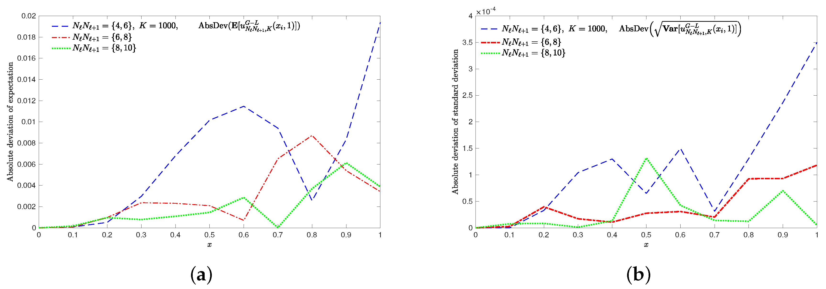
Computations were carried out at time $t=1$ along the spatial domain $[0,1]$ considering the set of points $x_i=ih$, $0\le i\le n=10$, $h=0.1$, fixing the number of realizations $K=1000$ and increasing the degree N of Laguerre polynomials from $N=4$ to $N=12$. The decrease of the RMSDs in Equations (91) and (92) is in full agreement with the results shown in Figure 5, where it is illustrated how the successive approximations of the absolute deviations for both the expectation and the standard deviation, defined as follows

$$\begin{array}{c}\hfill \begin{array}{ccc}\mathrm{AbsDev}\left(\mathbb{E}\left[u_{N_{\ell }{N}_{\ell +1},K}^{\mathrm{G}-\mathrm{L}}(x,t)\right]\right)\hfill & =& \left|\mathbb{E}\left[u_{N_{\ell +1},K}^{\mathrm{G}-\mathrm{L}}(x,t)\right]-\mathbb{E}\left[u_{N_{\ell },K}^{\mathrm{G}-\mathrm{L}}(x,t)\right]\right|,\hfill \\ \mathrm{AbsDev}\left(\sqrt{\mathrm{Var}\left[u_{N_{\ell }{N}_{\ell +1},K}^{\mathrm{G}-\mathrm{L}}(x,t)\right]}\right)\hfill & =& \left|\sqrt{\mathrm{Var}\left[u_{N_{\ell +1},K}^{\mathrm{G}-\mathrm{L}}(x,t)\right]}-\sqrt{\mathrm{Var}{[}_{N_{\ell },K}^{\mathrm{G}-\mathrm{L}}(x,t)]}\right|,\hfill \end{array}\end{array}$$

(93)

have a decreasing trend as N increases.

Figure 5. (a) Comparative graphics of the absolute deviations for successive approximations to the expectation $\mathbb{E}\left[u_{N_{\ell }{N}_{\ell +1},K}^{\mathrm{G}-\mathrm{L}}(x_i,1)\right]$ (Equation (93)). (b) Comparative graphics of the absolute deviations for successive approximations to the standard deviation $\sqrt{\mathrm{Var}\left[u_{N_{\ell }{N}_{\ell +1},K}^{\mathrm{G}-\mathrm{L}}(x_i,1)\right]}$ (Equation (93)). Both graphics correspond to the time $t=1$ on the spatial interval $0\le x\le 1$, $K=1000$ realizations and the degrees $N=\{4,6,8,10\}$ for the Laguerre polynomials.

5. Conclusions

This paper proposes an efficient numerical method to approximate the stochastic process solution of random hyperbolic models of telegraph type by a low order finite sum. This expression makes manageable the computational complexity of its statistical moments. The method combines the random Fourier transform approach and random Gaussian quadrature technique together with Monte Carlo method. The role of Gaussian quadrature is related to the approximation of the inverse Fourier transform while the Monte Carlo method provides the approximation of random ordinary differential transformed problem. Both cases, the random constant coefficient and the heterogeneous case, with random coefficient are treated and illustrated with numerical examples. Numerical experiments varying the degree of Gaussian quadrature and the amount of Monte Carlo simulations are discussed. The fact that the solution of the intermediate ODE problem is solved using Monte Carlo, and that the random inverse Fourier transform is approximated using quadratures allows an easy computation that can be checked with real experiments and applicable to real problems, even outside of our telegraph type hyperbolic models.

References

- Casabán, M.C.; Company, R.; Cortés, J.C.; Jódar, L. Solving the random diffusion model in an infinite medium: A mean square approach. Appl. Math. Model. 2014, 38, 5922–5933. [Google Scholar] [CrossRef] [Scilit]
- Casabán, M.C.; Cortés, J.C.; Jódar, L. Solving random mixed heat problems: A random integral transform approach. J. Comput. Appl. Math. 2016, 291, 5–19. [Google Scholar] [CrossRef] [Scilit]
- Casabán, M.C.; Cortés, J.C.; Jódar, L. Analytic-Numerical solution of random parabolic models: A mean square Fourier transform approach. Math. Model. Anal. 2018, 23, 79–100. [Google Scholar] [CrossRef] [Scilit]
- Farlow, S.J. Partial Differential Equations for Scientists and Engineers; John Wiley & Sons: New York, NY, USA, 1993. [Google Scholar]
- Saadatmandi, A.; Dehghan, M. Numerical solution of hyperbolic telegraph equation using the Chebyshev tau method. Numer. Meth. Part. Differ. Equ. 2010, 26, 239–252. [Google Scholar] [CrossRef] [Scilit]
- Weston, V.H.; He, S. Wave splitting of the telegraph equation in ℝ3 and its application to inverse scattering. Inverse Probl. 1993, 9, 789–812. [Google Scholar] [CrossRef] [Scilit]
- Jordan, P.M.; Puri, A. Digital signal propagation in dispersive media. J. Appl. Phys. 1999, 85, 1273–1282. [Google Scholar] [CrossRef] [Scilit]
- Banasiak, J.; Mika, J.R. Singularly perturved telegraph equations with applications in the random walk theory. J. Appl. Math. Stoch. Annal. 1998, 11, 9–28. [Google Scholar] [CrossRef] [Scilit]
- Pozar, D.M. Microwave Engineering, 2nd ed.; John Wiley & Sons, Inc.: New York, NY, USA, 1998. [Google Scholar]
- Kac, M. A stochastic model related to the telegrapher’s equation. Rocky Mt. J. Math. 1974, 4, 497–509. [Google Scholar] [CrossRef] [Scilit]
- Iacus, S.M. Statistical analysis of the inhomogeneous telegrapher’s process. Stat. Probab. Lett. 2001, 55, 83–88. [Google Scholar] [CrossRef] [Scilit]
- Kolesnik, A.D. Moment analysis of the telegraph random process. Bull. Acad. Sci. Mold. Ser. Math. 2012, 68, 90–107. [Google Scholar]
- Soong, T.T. Random Differential Equations in Science and Engineering; Academic Press: New York, NY, USA, 1973. [Google Scholar]
- Casabán, M.C.; Cortés, J.C.; Jódar, L. A random Laplace transform method for solving random mixed parabolic differential problems. Appl. Math. Comput. 2015, 259, 654–667. [Google Scholar] [CrossRef] [Scilit]
- Casabán, M.C.; Cortés, J.C.; Jódar, L. Solving linear and quadratic random matrix differential equations using: A mean square approach. The non-autonomous case. J. Comput. Appl. Math. 2018, 330, 937–954. [Google Scholar] [CrossRef] [Scilit]
- Casabán, M.C.; Cortés, J.C.; Jódar, L. Solving linear and quadratic random matrix differential equations: A mean square approach. Appl. Math. Model. 2016, 40, 9362–9377. [Google Scholar] [CrossRef] [Scilit]
- Kroese, D.P.; Taimre, T.; Botev, Z.I. Handbook of Monte Carlo Methods; Wiley Series in Probability and Statistics; John Wiley & Sons: New York, NY, USA, 2011. [Google Scholar]
- Wolfram Research, Inc. Mathematica, version 11.3; Wolfram Research, Inc.: Champaign, IL, USA, 2018. [Google Scholar]
- Abramowitz, M.; Stegun, I.A. Handbook of Mathematical Functions with Formulas, Graphs, and Mathematical Tables; Dover Publications, Inc.: New York, NY, USA, 1972. [Google Scholar]
- Polyanin, A.D.; Zaitsev, V.F. Handbook of Nonlinear Partial Differential Equations; Chapman & Hall: New York, NY, USA, 2004. [Google Scholar]
© 2019 by the authors. Licensee MDPI, Basel, Switzerland. This article is an open access article distributed under the terms and conditions of the Creative Commons Attribution (CC BY) license (http://creativecommons.org/licenses/by/4.0/).