Dynamic Analysis of Sugarcane Pokkah Boeng Model with Time Delay in Removal or Chemical Control

Abstract

In this paper, a sugarcane pokkah boeng SEIR model with time delay due to removal or chemical treatment of diseased sugarcane plants is investigated. By analyzing the characteristic equations, the stability of each feasible equilibrium of the system is discussed, and the existence of a Hopf bifurcation at the positive equilibrium is established. Furthermore, by choosing the delay as a bifurcation parameter, we show that Hopf bifurcations can occur as $\tau$ crosses some critical values. Meanwhile, we adopt a hierarchical Bayesian model to conduct statistical inference on time delay and combine it with the former to carry out an empirical analysis on the prevention and control of sugarcane pokkah boeng. These provide a more comprehensive and effective theoretical basis for decision-making in the prevention and control of sugarcane pokkah boeng. Numerical simulations are carried out to illustrate the main theoretical results.

1. Introduction

Sugarcane is the world’s largest commercial crop, which is cultivated in more than 120 countries on approximately 26.27 million hectares, with a global harvest of 1.9 billion tonnes [1]. Approximately 80% of the world’s sugar is derived from sugarcane [2,3]. Unfortunately, various diseases caused by fungi, bacteria, viruses, and phytoplasmas severely affect sugarcane productivity worldwide. No country is immune to the adverse effects of sugarcane diseases [4].

Sugarcane pokkah boeng (PB), alternatively referred to as twisted top disease (TTD), is a fungal disease affecting sugarcane caused by multiple Fusarium species. It primarily targets the apical and tender tissues, inducing twisting and deformation of the top leaves. In severe cases, it can lead to necrosis and rot of young heart leaves at the apex, with diseased plants exhibiting shortened internodes; extreme infections may even cause the entire plant to wither and die, significantly impairing yield and sugar accumulation, rendering crops economically valueless, and resulting in substantial losses [5,6].

While previous studies hold diverse views on PB transmission, aerial dispersal is widely recognized as its primary pathway [7,8,9]. Common control measures (including monitoring, chemical use, resistant breeding, and integrated management) have inherent limitations: chemicals effectively inhibit pathogens but induce drug resistance with long-term application, and despite progress in resistant breeding, its promotion is hampered by insufficient genetic resources and poor adaptability, necessitating optimized strategies [10,11,12,13]. Notably, scientific field management and human intervention (regular field surveys, timely removal of infected plants, targeted pesticide spraying) are indispensable; when combined with rational chemical use, these measures can effectively curb PB outbreaks [6]. Thus, developing targeted mathematical models to analyze PB’s epidemic dynamics is crucial for supporting human intervention strategy formulation.

To better model the transmission dynamics of PB, we construct a time-delay SEIR model that incorporates the critical lag between pathogen detection and the implementation of control measures. As an extension of the classical SIR compartmental model, the SEIR framework is supported by foundational studies [14,15,16], with recent frontier applications reported in the literature [17,18,19].

Specifically, informed by the actual field delay in responding to detected infected sugarcane plants, we introduce a time lag $\tau$ into the SEIR model to more realistically represent PB transmission dynamics. However, accurately estimating this key parameter remains challenging due to field variability and data scarcity. To address this, we employ a Hierarchical Bayesian Model (HBM). HBMs are well-suited for this task as they mitigate over-reliance on priors through hyperparameters, improve estimation accuracy, and robustly handle uncertainty and limited data [20,21]. We compute the HBM posterior distributions using Markov Chain Monte Carlo (MCMC) methods, such as Metropolis–Hastings and Gibbs sampling, which enable inference for complex models. Finally, we validate the HBM-inferred $\tau$ within the time-delay SEIR framework and conduct an empirical control analysis, creating a mutually reinforcing research cycle.

The rest of this paper is organized as follows. In Section 2, the SEIR transmission model for sugarcane PB boeng with time delay is proposed. In Section 3, the basic reproduction number of the model is calculated, and the asymptotic stability of the disease-free equilibrium is discussed. In Section 4, the stability and Hopf bifurcation of the PB disease equilibrium are analyzed, and the critical values of the time delay are derived under specific parameter conditions based on statistical data. In Section 5, via the construction of the Bayesian hierarchical model, the statistical inference on time delay is given. Finally, the corresponding prevention and control of sugarcane PB is discussed according to the practical dynamic behaviors from the oscillations of disease spreading, and the internal laws of PB dissemination are elucidated by combining the obtained results with numerical simulations; some conclusions are given.

2. SEIR Transmission Model for Sugarcane PB

Based on the core structure of the classic SEIR (Susceptible-Exposed-Infectious-Recovered) model, we establish a transmission model for sugarcane PB. This study focuses on a field sugarcane population comprising N individual plants (corresponding to the sugarcane population in a specific planting area). These N sugarcane plants are treated as individual units in the model to simulate the disease transmission process within the population.

According to the infection stages and transmission status of sugarcane plants with respect to the pathogen causing PB, the sugarcane plants in the population are divided into four categories, each corresponding to a different health status, as follows:

S (Susceptible): The number of susceptible sugarcane plants that have not been exposed to the PB pathogen. These plants are free from pathogen infection and are susceptible to infection.

E (Exposed): The number of exposed sugarcane plants that have been in contact with the pathogen but show no symptoms. These plants are infected with the pathogen but have not yet exhibited PB symptoms (such as shoot rot and yellowing of heart leaves) and temporarily lack the ability to transmit the disease.

I (Infectious): The number of infectious sugarcane plants that show symptoms and can transmit the pathogen. These plants display typical PB symptoms, carry viable pathogens, and can spread the disease through air currents, rainwater, or agricultural operations.

R (Removed/Recovered): The number of sugarcane plants that have been removed or recovered. These plants have been manually removed or recovered after chemical control, and they no longer participate in disease transmission.

If we let $N\left(t\right)$ be the total number of sugarcane plants at time t, then we have the equation:

$$N\left(t\right)=S\left(t\right)+E\left(t\right)+I\left(t\right)+R\left(t\right).$$

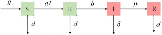
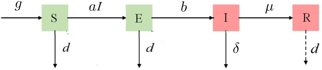
For the SEIR transmission process of sugarcane PB, Figure 1 can clearly show the complete transmission path and transformation relationship from susceptible plants to exposed plants and infectious plants, and then to removed/recovered plants.

Figure 1. Structure of sugarcane PB SEIR spreading process.

And the transmission rules of the model are summarized as follows:

(i) Two ways for infectious plants I to turn into removed/recovered plants R are integrated into a unified framework. The first is spatial isolation: clearing infected plants I blocks the pathogen’s spread, stops infectious plants I from contacting susceptible ones, and thus turns them into R. The second is chemical control: spraying fungicides, accompanied by pruning diseased shoots, makes infectious plants I lose infectivity quickly and become R faster.

(ii) To better reflect field realities, a time delay $\tau$ is introduced into the SEIR model. This delay represents the interval between the detection of infected plants and the implementation of control measures, such as manual removal or chemical treatment. Incorporating this delay enhances the model’s ability to accurately capture the disease transmission dynamics.

(iii) Infectious sugarcane plants I generally remain infectious even after death, and such dead plants are considered together with living infectious plants. Field survey results from Viswanathan et al. [12] and Siva et al. [6] show that dead plants infected with sugarcane PB contribute approximately 15–20% of the total pathogen transmission in the field, thus representing a non-negligible source of infection.

This feature is absent from conventional SEIR models. Furthermore, we define a very small parameter $\delta$ as the probability that an infectious plant, upon dying without being removed, simultaneously loses its infectivity. This contrasts with the majority of infectious plant deaths, which do not entail such a loss.

(iv) Other key parameters in the model, adapted to the characteristics of sugarcane PB, are defined as follows:

a: Pathogen infection rate coefficient—The probability that a susceptible plant S is infected by the pathogen from an infectious plant I via vectors, which is affected by field humidity and planting density.

b: Conversion rate from exposed period to infectious period—The rate at which exposed plants E develop into symptomatic infectious plants I, which is positively correlated with temperature (with the rate peaking at 25–32°C).

d: Natural mortality rate—The normal death rate of sugarcane unrelated to the disease (caused by other factors such as senescence and insect pests). Note that in the R stage: if it refers to removed plants, there is no mortality rate; if it refers to recovered ones, their mortality rate is assumed to be d. According to the above definition of $\delta$, it can be considered that $d>\delta$.

g: Germination rate of sugarcane seedlings or average replanting rate of seedlings—Related to the efficiency of agricultural management.

$\mu$: Removal rate due to disease (including the effect of chemical control)—The rate at which infectious plants are transformed into category R plants after manual uprooting or pesticide spraying following a time delay $\tau$.

According to the above rules, the dynamics of the PB propagation model SEIR are governed by the following nonlinear ordinary differential system:

$$\begin{array}{c}\left\{\begin{array}{c}{\displaystyle \frac{\mathrm{d}S\left(t\right)}{\mathrm{d}t}}=g-aS\left(t\right)I\left(t\right)-dS\left(t\right),\hfill \\ {\displaystyle \frac{\mathrm{d}E\left(t\right)}{\mathrm{d}t}}=aS\left(t\right)I\left(t\right)-bE\left(t\right)-dE\left(t\right),\hfill \\ {\displaystyle \frac{\mathrm{d}I\left(t\right)}{\mathrm{d}t}}=bE\left(t\right)-\mu I(t-\tau )-\delta I\left(t\right),\hfill \\ {\displaystyle \frac{\mathrm{d}R\left(t\right)}{\mathrm{d}t}}=\mu I(t-\tau )-dR\left(t\right),\hfill \end{array}\right.\hfill \end{array}$$

(1)

where $0\le a,b,d,g,\mu ,\delta \le 1$, $\delta <d$ and $\tau \ge 0$. Namely, there are a total of 7 parameters in the model (1) at this time.

Obviously, for system (1), the fourth equation can be decoupled from the first three equations. That is to say, substituting the solutions obtained from the first three equations into the fourth equation allows us to determine the fourth unknown function $R\left(t\right)$. Therefore, we firstly consider the three-dimensional reduced form of system (1) as follows

$$\begin{array}{c}\left\{\begin{array}{c}{\displaystyle \frac{\mathrm{d}S\left(t\right)}{\mathrm{d}t}}=g-aS\left(t\right)I\left(t\right)-dS\left(t\right),\hfill \\ {\displaystyle \frac{\mathrm{d}E\left(t\right)}{\mathrm{d}t}}=aS\left(t\right)I\left(t\right)-bE\left(t\right)-dE\left(t\right),\hfill \\ {\displaystyle \frac{\mathrm{d}I\left(t\right)}{\mathrm{d}t}}=bE\left(t\right)-\mu I(t-\tau )-\delta I\left(t\right).\hfill \end{array}\right.\hfill \end{array}$$

(2)

It should be noted that the variables $S\left(t\right)$, $E\left(t\right)$, $I\left(t\right)$, $R\left(t\right)$ represent the numbers of sugarcane individuals in different compartments; therefore, they must remain biologically non-negative at all times. Moreover, the total population of sugarcane is biologically bounded due to limited planting area and natural growth constraints.

To determine the existence of equilibrium, we let the right side of the system (1) equal zero; a direct calculation shows that there are at most two equilibrium points. Then system (2) always has an equilibrium $P_0({\displaystyle \frac{g}{d}},0,0)$, which corresponds to the disease-free equilibrium. And if the following condition holds:

$$\begin{array}{c}{\mathrm{H}}_1:abg-dm(b+d)>0,\hfill \end{array}$$

then the other equilibrium of system (2) is a positive one, namely a endemic equilibrium $P_1(S^{*},E^{*},I^{*})$ with

$$\begin{array}{c}\{S^{*}={\displaystyle \frac{m(b+d)}{ab}},E^{*}={\displaystyle \frac{abg-dm(b+d)}{ab(b+d)}},I^{*}={\displaystyle \frac{abg-dm(b+d)}{am(b+d)}}\}\hfill \end{array}$$

(3)

where $m=\mu +\delta$ denotes the total removal rate of infected individuals, which includes the chemical/manual removal rate $\mu$ and the infectious mortality (death with infectivity loss) $\delta$; then the endemic equilibrium value R in system (1) becomes $R^{*}={\displaystyle \frac{\mu (abg-dm(b+d\left)\right)}{adm(b+d)}}$.

3. Basic Reproductive Number and Stability of Disease-Free Equilibrium

The basic reproductive number plays an important role in the dynamic analysis of online disease propagation. It can be used to reveal the average number of new infections caused by infected individuals during the disease propagation. Obviously, for system (2), the disease-free equilibrium point $P_0=({\displaystyle \frac{g}{d}},0,0)$, which implies that in a certain state, there will be no disease propagation within a certain area.

Next, we compute the basic reproductive number by applying the method of the next generation matrix, which is defined by linearizing the system at the disease-free equilibrium $P_0$. Combining the forms of the second and third equations of system (2), we decompose the system equations into new infection terms and transition terms, compute the partial derivative matrices at the disease-free equilibrium $P_0$, yielding

$$\begin{array}{c}F=\left(\begin{array}{cc}{\displaystyle \frac{ag}{d}}& 0\\ 0& 0\end{array}\right),V=\left(\begin{array}{cc}b+d& 0\\ -b& \delta +\mu e^{-\lambda \tau }\end{array}\right).\hfill \end{array}$$

where the intermediate matrix V contains the $e^{-\lambda \tau }$ term, which is a direct result of the linearization of the delayed removal term $\mu I(t-\tau )$ in the infectious compartment $I\left(t\right)$, and reflects the impact of the time-delay effect on the state transition of infectious individuals. Correspondingly, we can get the next-generation matrix

$$\begin{array}{c}F{V}^{-1}=\left(\begin{array}{cc}{\displaystyle \frac{ag}{d(b+d)}}& 0\\ 0& 0\end{array}\right).\hfill \end{array}$$

The spectral radius of $F{V}^{-1}$ is defined as the basic reproductive number $R_0$ of system (2), which is similar to that in epidemic models and is independent of $\lambda$ and $\tau$ due to the direct matrix inversion and spectral radius calculation, and we have

$$\begin{array}{c}{R}_0=\rho \left(F{V}^{-1}\right)={\displaystyle \frac{ag}{d(b+d)}}.\hfill \end{array}$$

(4)

Therefore, if (H₁) holds, namely under the existence condition of $P_1$, then basic reproductive number $R_0>{\displaystyle \frac{m}{b}}$; if the following holds:

$$\begin{array}{c}{\mathrm{H}}_2:abg-dm(b+d)<0,\hfill \end{array}$$

then basic reproductive number $R_0<{\displaystyle \frac{m}{b}}$. Thus, we can obtain a basis for judgment of the basic reproductive number $R_0<1$ or $R_0>1$ by verifying whether ${\displaystyle \frac{m}{b}}$ is greater than 1.

Furthermore we analyze the local stability of system (2) at the disease-free equilibrium $P_0=({\displaystyle \frac{g}{d}},0,0)$. The Jacobian matrix at the disease-free equilibrium $P_0$ of system (2) with $\tau =0$ is given as

$$J\left(P_0\right)=\left(\begin{array}{ccc}-d& 0& -{\displaystyle \frac{ag}{d}}\\ 0& -b-d& {\displaystyle \frac{ag}{d}}\\ 0& b& -\delta -\mu \end{array}\right).$$

The corresponding characteristic equation at $P_0$ can be calculated as

$$\begin{array}{c}(\lambda +d)f\left(\lambda \right)=0,\hfill \end{array}$$

where $f\left(\lambda \right)=(b+d+\lambda )\left(\delta +\lambda +\mu e^{-\lambda \tau }\right)-{\displaystyle \frac{abg}{d}}.$ It is clear that one eigenvalue of the characteristic equation is $\lambda =-d<0$. If (H₁) holds, it is easy to show that, for real $\lambda$,

$$f\left(0\right)=(b+d)(\delta +\mu )-{\displaystyle \frac{abg}{d}}<0,{lim}_{\lambda \to +\infty }f\left(\lambda \right)=+\infty .$$

Hence, $f\left(\lambda \right)=0$ has at least one positive real root. Therefore, if (H₁) holds, then the equilibrium $P_0$ is unstable for all $\tau \ge 0$.

If ${\mathrm{H}}_2:abg-dm(b+d)<0$ holds, then it is easy to show that $f\left(0\right)>0$. And by the Routh–Hurwitz criterion, under the condition of H₂, we can verify that the equilibrium $P_0$ is locally asymptotically stable when $\tau =0$. The case of $\tau >0$ requires further analysis but is not discussed here, as the main focus is on the endemic equilibrium $P_1$.

Therefore, we can obtain the following results:

Theorem 1. 

For system (2), we have the following:

(i) 

If (H₁) and $m>b$ hold, then basic reproductive number $R_0>1$; if (H₂) and $m<b$ hold, then basic reproductive number $R_0<1$.

(ii) 

If (H₁) holds, then the disease-free equilibrium $P_0({\displaystyle \frac{g}{d}},0,0)$ is unstable for all $\tau \ge 0$; if (H₂) holds, then it is locally asymptotically stable for $\tau =0$.

4. Stability of Endemic Equilibrium and Hopf Bifurcation

Now we investigate the stability and bifurcated periodic solutions at the positive equilibrium $P_1(S^{*},E^{*},I^{*})$ of system (2), i.e., the endemic equilibrium. In particular, the introduction of time delay will affect the dynamic behavior of the model, possibly leading to complex dynamic phenomena such as stability switches or Hopf bifurcations. This is of great significance for understanding the transmission rules of sugarcane diseases and formulating prevention and control strategies.

The Jacobian matrix of system (2) linearized at the endemic equilibrium $P_1(S^{*},E^{*},I^{*})$ is given by

$$J\left(P_1\right)=\left(\begin{array}{ccc}-a{I}^{*}-d& 0& -a{S}^{*}\\ a{I}^{*}& -(b+d)& a{S}^{*}\\ 0& b& -\mu e^{-\lambda \tau }-\delta \end{array}\right).$$

The corresponding characteristic equation is

$$\begin{array}{c}(\lambda +b+d)\left(\lambda +{\displaystyle \frac{abg}{m(b+d)}}\right)\left(\lambda +\delta +\mu e^{-\lambda \tau }\right)-(\lambda +d)m(b+d)=0.\hfill \end{array}$$

(5)

where $\delta =m-\mu$. Expanding (5) yields the transcendental characteristic equation

$$\begin{array}{c}f:={\lambda }^3+{\xi }_2{\lambda }^2+{\xi }_1\lambda +{\xi }_0+({\eta }_2{\lambda }^2+{\eta }_1\lambda +{\eta }_0)e^{-\lambda \tau }=0,\hfill \end{array}$$

(6)

where

$$\begin{array}{c}{\xi }_2=b+d+{\displaystyle \frac{abg}{m(b+d)}}+m-\mu ,\hfill \\ {\xi }_1=(b+d){\displaystyle \frac{abg}{m(b+d)}}+(b+d)(m-\mu )+{\displaystyle \frac{abg}{m(b+d)}}(m-\mu )-m(b+d),\hfill \\ {\xi }_0=(b+d){\displaystyle \frac{abg}{m(b+d)}}(m-\mu )-m(b+d){\displaystyle \frac{abg}{m(b+d)}},\hfill \\ {\eta }_2=\mu ,\hfill \\ {\eta }_1=\mu \left(b+d+{\displaystyle \frac{abg}{m(b+d)}}\right),\hfill \\ {\eta }_0=\mu (b+d){\displaystyle \frac{abg}{m(b+d)}}.\hfill \end{array}$$

When $\tau =0$, (6) becomes

$$\begin{array}{c}(\lambda +b+d)\left(\lambda +{\displaystyle \frac{abg}{m(b+d)}}\right)\left(\lambda +m\right)-(\lambda +d)m(b+d)=0.\hfill \end{array}$$

And by the Routh–Hurwitz criterion, under the existence condition of $P_1$: H₁, we can verify that the equilibrium $P_1$ is locally asymptotically stable when $\tau =0$.

To investigate the possibility of a Hopf bifurcation, we substitute $\lambda =\mathbf{i}\omega$ ($\omega >0$) into the characteristic Equation (5). Separating the real and imaginary parts gives the system

$$\begin{array}{c}\mu (b+d)(abg-m{\omega }^2)cos\omega \tau +\mu \omega (abg+m{(b+d)}^2)sin\omega \tau =p_1\left(\omega \right)\hfill \\ \mu (b+d)(abg-m{\omega }^2)sin\omega \tau -\mu \omega (abg+m{(b+d)}^2)cos\omega \tau =p_2\left(\omega \right)\hfill \end{array}$$

(7)

where

$$\begin{array}{c}{p}_1\left(\omega \right)=abg\left[(b+d)(\mu -m)+{\omega }^2\right]+m(b+d)\left[(b+d)(dm+{\omega }^2)+{\omega }^2(m-\mu )\right],\hfill \\ p_2\left(\omega \right)=\omega \left[abg(b+d-\mu +m)-m(b+d)\left((b+d)\mu +{\omega }^2\right)\right].\hfill \end{array}$$

Squaring and adding the two equations in (7) eliminates the trigonometric terms and yields a polynomial equation in ${\omega }^2$:

$$\begin{array}{c}{q}_0+q_1{\omega }^2+q_2{\omega }^4+{\omega }^6=0,\hfill \end{array}$$

(8)

where the coefficients $q_0,q_1,q_2$ are given by

$$\begin{array}{c}{q}_0=[{\displaystyle \frac{abg}{m}}-d(b+d)][abg(m-2\mu )-d{m}^2(b+d)],\hfill \\ q_1=2dm(b+d)(b+d-\mu +m)-2abg(b-\mu +m)+{\displaystyle \frac{a^2{b}^2{g}^2\left({(b+d)}^2+m(m-2\mu )\right)}{m^2{(b+d)}^2}},\hfill \\ q_2={\displaystyle \frac{a^2{b}^2{g}^2}{m^2{(b+d)}^2}}+{(b+d+m)}^2-2\mu m.\hfill \end{array}$$

Under the existence condition of the endemic equilibrium $P_1$, i.e., H₁: $abg-dm(b+d)>0$, it follows from (3) that

$$\begin{array}{c}g>{\displaystyle \frac{d(b+d)m}{ab}},\hfill \end{array}$$

(9)

Moreover, if $q_0>0$, which is equivalent to

$$abg(m-2\mu )-d{m}^2(b+d)>0,$$

then we obtain the sufficient condition

$$\begin{array}{c}\mu <{\displaystyle \frac{m\left(abg-bdm-d^{2}m\right)}{2abg}}<{\displaystyle \frac{m}{2}},\hfill \end{array}$$

(10)

at this time, we can verify that $q_2>0$ holds, and $q_1>0$ also holds as a quadratic polynomial in g. Hence, if $q_0>0$, (8) has no positive real roots. Accordingly, by Theorem 3.4.1 in [22], we see that if $q_0>0$, i.e., (9) and (10) hold, then $P_1$ is locally asymptotically stable for all $\tau \ge 0$. If $q_0<0$ holds, then (8) has a unique positive root ${\omega }_0$, that is, (8) has a pair of purely imaginary roots of the form $\mathbf{i}{\omega }_0$. Denote

$$\begin{array}{c}{\tau }_{0n}={\displaystyle \frac{1}{{\omega }_0}}arccos{\displaystyle \frac{N_1+abg{m}^2{(b+d)}^2(bd+d^2+{\omega }_0^2)-a^2{b}^2{g}^2(m-\mu )[{(b+d)}^2+{\omega }_0^2]}{\mu [{(b+d)}^2+{\omega }_0^2][a^2{b}^2{g}^2+m^2{\omega }_0^2{(b+d)}^2]}}+{\displaystyle \frac{2n\pi }{{\omega }_0}},\hfill \end{array}$$

(11)

where $N_1=m^2{\omega }_0^2{(b+d)}^2[b^2\mu -bd(m-2\mu )-(d^2+{\omega }_0^2)(m-\mu )],n=0,1,2\dots$. By Theorem 3.4.1 in [22] we see that if $q_0<0$, then $P_1$ remains stable for $\tau \le {\tau }_{00}:={\tau }_0$.

We now claim that

$${\left[{\displaystyle \frac{\mathrm{d}\left(\mathrm{Re}\lambda \right)}{\mathrm{d}\tau }}\right]}_{\tau ={\tau }_0}>0.$$

This will show that there exists at least one eigenvalue with a positive real part for $\tau >{\tau }_0$. Moreover, the conditions for the existence of a Hopf bifurcation are then satisfied, yielding a periodic solution. To this end, differentiating (6) with respect to $\tau$, it follows that

$$\begin{array}{c}{\left[{\displaystyle \frac{\mathrm{d}\lambda }{\mathrm{d}\tau }}\right]}^{-1}={\displaystyle \frac{2{\eta }_2\lambda +{\eta }_1}{\lambda \left({\eta }_2{\lambda }^2+{\eta }_1\lambda +{\eta }_0\right)}}-{\displaystyle \frac{3{\lambda }^2+2{\xi }_2\lambda +{\xi }_1}{\lambda \left({\lambda }^3+{\xi }_2{\lambda }^2+{\xi }_1\lambda +{\xi }_0\right)}}-{\displaystyle \frac{{\tau }_0}{\lambda }}.\hfill \end{array}$$

Hence, a direct calculation shows that

$$\begin{array}{c}\mathrm{sgn}{\left[{\displaystyle \frac{\mathrm{d}\left(\mathrm{Re}\lambda \right)}{\mathrm{d}\tau }}\right]}_{\lambda =\mathbf{i}{\omega }_0}=\mathrm{sgn}{\left\{\mathrm{Re}{\left[{\displaystyle \frac{\mathrm{d}\lambda }{\mathrm{d}\tau }}\right]}^{-1}\right\}}_{\lambda =\mathbf{i}{\omega }_0}.\hfill \end{array}$$

(12)

We derive from (12) that

$$\begin{array}{c}\mathrm{sgn}{\left[{\displaystyle \frac{\mathrm{d}\left(\mathrm{Re}\lambda \right)}{\mathrm{d}\tau }}\right]}_{\lambda =\mathbf{i}{\omega }_0}=\mathrm{sgn}\left\{{\displaystyle \frac{2{\omega }_0^2({\xi }_2^2-2{\xi }_1-{\eta }_2^2)-{\eta }_1^2+2{\eta }_0{\eta }_2+{\xi }_1^2-2{\xi }_0{\xi }_2+3{\omega }_0^4}{{\eta }_1^2{\omega }_0^2+{({\eta }_0-{\eta }_2{\omega }_0^2)}^2}}\right\}>0.\hfill \end{array}$$

(13)

Therefore, the transversal condition holds, and a Hopf bifurcation occurs at $\omega ={\omega }_0,\tau ={\tau }_0$. In conclusion, the following results are obtained.

Therefore, we can obtain the following results:

Theorem 2. 

For system (2), suppose that the endemic equilibrium $P_1$ exists (i.e., ${\mathrm{H}}_1$ holds) and that condition (10) is satisfied. Then there exists a sequence of critical delay values

$$0<{\tau }_0<{\tau }_{01}<\cdots <{\tau }_{0k}<\cdots$$

such that the characteristic Equation (6) has a pair of purely imaginary roots $\pm \mathbf{i}{\omega }_0$ at $\tau ={\tau }_{0k}$. Moreover, if the transversality condition

$${\displaystyle \frac{\mathrm{d}}{\mathrm{d}\tau }}\left(\mathrm{Re}\lambda \left(\tau \right)\right){|}_{\tau ={\tau }_{0k},\lambda =\mathbf{i}{\omega }_0}>0$$

holds, then a Hopf bifurcation occurs at $\tau ={\tau }_{0k}$. In particular, the endemic equilibrium $P_1$ is locally asymptotically stable when $0\le \tau <{\tau }_0$ and unstable when $\tau >{\tau }_0$, with a family of periodic solutions bifurcating from $P_1$ for τ sufficiently close to ${\tau }_0$.

Next, we are interested in practically relevant solutions of the system, and choose the specific parameter values of $g,a,b,d,\delta$ and $\mu$ in system (2) of the original model (1), which can be obtained from some existing literature or the real statistical and estimated ranges, as shown in Table 1. When the specific values of other parameters are given as follows:

$$\begin{array}{c}\{g,a,b,d,\delta \}=\left\{{\displaystyle \frac{53}{2000}},{\displaystyle \frac{11}{50}},{\displaystyle \frac{11}{30}},{\displaystyle \frac{1}{200}},{\displaystyle \frac{1}{1000}},{\displaystyle \frac{3}{5}}\right\},\hfill \\ \mathit{i}.\mathit{e}.,\{0.0265,0.22,0.367,0.005,0.001\},\hfill \end{array}$$

(14)

and we retain only $\mu$ as the undetermined parameter. Then $\tau$ can be determined by $\mu$ according to (8) and (11), where $q_0,q_1$ and $q_2$ in (8) are given by

$$\begin{array}{c}{q}_0={\displaystyle \frac{(223000\mu -256297)\left(223000000{\mu }^2+256966000\mu -256297\right)}{14400000000000000(1000\mu +1)}},\hfill \\ q_1={\displaystyle \frac{6199067953000000000{\mu }^3-7164658863161000000{\mu }^2-14051803633381000\mu +20444950552307733}{4475610000000000{(1000\mu +1)}^2}},\hfill \\ q_2={\displaystyle \frac{111890250000000000{\mu }^4-82947972000000000{\mu }^3-15705599263750000{\mu }^2-31161907050500\mu -3716930577649}{111890250000{(1000\mu +1)}^2}}.\hfill \end{array}$$

Table 1. Model parameters and descriptions for the sugarcane PB SEIR model.

Para	Value	Description	Range / Reference
g	0.0265	Sprouting rate of newly planted sugarcane	[4]
a	0.22	Transmission rate of the pathogen to susceptible sugarcane plants via vectors	[0.1, 0.3]
b	0.3667	Conversion rate from exposed period to infectious period	[0.3, 0.5]
d	0.005	Natural mortality rate	[0.001, 0.01]
$\delta$	0.001	Probability that an infected plant dies without being removed or loses infectivity	[0, 0.002]
$\mu$	–	Removal rate due to disease	[0.2, 0.95]

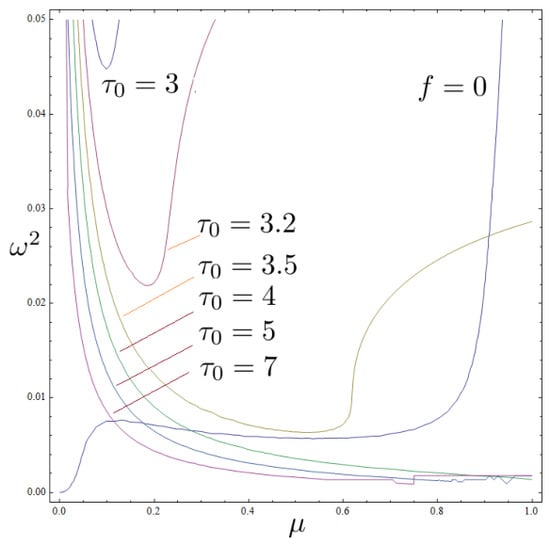
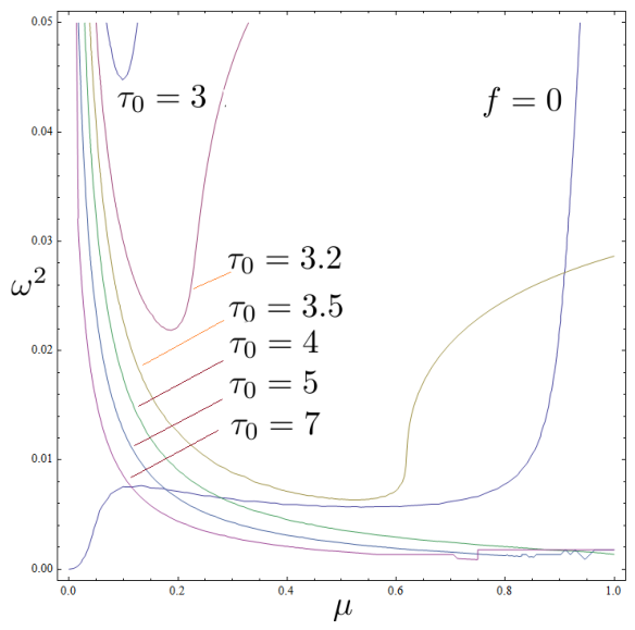
In fact, we can plot the contour graphs of (11) and the function curve of $f=0$ based on (8), as shown in Figure 2. It can be seen that with the increase in $\mu$, the critical delay value ${\tau }_0$ of the Hopf bifurcation becomes smaller and smaller. That is, under the given conditions, a higher removal rate of diseased plants leads to a shorter delay in periodic outbreaks. This result is somewhat inconsistent with practical observations, likely due to the influence of other habitat-related parameters.

Figure 2. The corresponding function curves of ${\omega }^2$ in $\mu$ by setting ${\tau }_0=3,3.2,3.5,4,5,7$ and the intersection points $({\omega }_0^2,\mu )$ between them and the curve of $f=0$ respectively.

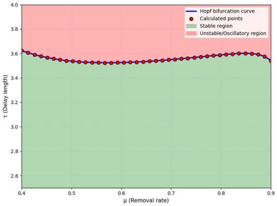
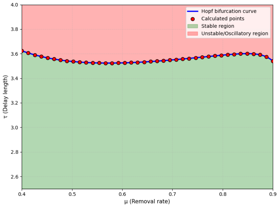
Next, we select the parameter set (14) and treat the removal rate $\mu$ and the time delay $\tau$ as free variables. A Hopf bifurcation diagram for system (2) can then be numerically plotted in the ($\mu$, $\tau$) plane, as shown in Figure 3. This figure presents the Hopf bifurcation curve and indicates the regions corresponding to an asymptotically stable equilibrium and a stable periodic solution.

Figure 3. Hopf bifurcation diagram in the ($\mu$, $\tau$) plane in system (2) under the parameter conditions (14), where only a portion of the bifurcation diagram is given.

To numerically validate Theorem 2, we employ the parameter set (14) from Table 1 and set $\mu =0.6$. Under this configuration, system (2) possesses a unique endemic equilibrium:

$$P_1=\left({\displaystyle \frac{134023}{48400}},{\displaystyle \frac{367491}{10793200}},{\displaystyle \frac{122497}{5897012}}\right)\approx (2.76907,0.0340484,0.0207727).$$

For $\tau =0$, all eigenvalues of the characteristic equation have negative real parts, indicating local asymptotic stability. Solving the polynomial Equation (8) yields ${\omega }_0\approx 0.322$ and the critical delay ${\tau }_0\approx 3.5279$. Moreover, the transversality condition is satisfied, i.e.,

$$\mathrm{sgn}{\left[{\displaystyle \frac{\mathrm{d}\left(\mathrm{Re}\lambda \right)}{\mathrm{d}\tau }}\right]}_{\lambda =\mathbf{i}{\omega }_0}>0.$$

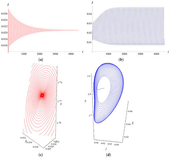
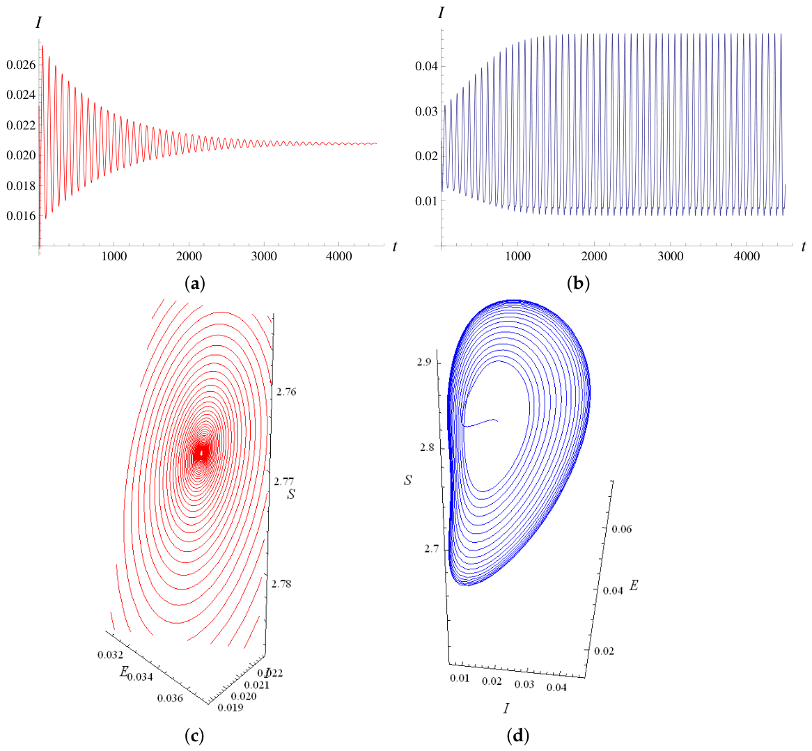
As shown in Figure 4, when $\tau =3.45<{\tau }_0$, the equilibrium $P_1$ remains stable (panels (a) and (c)). When $\tau =3.6>{\tau }_0$, a stable periodic solution emerges near $P_1$ (panels (b) and (d)), confirming the occurrence of a supercritical Hopf bifurcation.

Figure 4. Simulated time histories of I in system (2) for $\tau =3.45$ and $\tau =3.6$ under the initial conditions: (a) $(S,E,I)=(0,0,0.0025)$, (b) $(S,E,I)=(0,0,0.0025)$; trajectories near: (c) the asymptotically stable equilibrium, (d) an asymptotically stable periodic solution.

The numerical verification confirms ${\tau }_0\approx 3.5279$ days as a threshold for periodic dynamics. For $\tau =3.45<{\tau }_0$, the stable equilibrium reflects a controlled field scenario: timely intervention (within 3.5 days) suppresses outbreaks. For $\tau =3.6>{\tau }_0$, stable periodic solutions emerge, indicating recurrent PB outbreaks driven by excessive control delays. These results underscore the need to maintain response delays below ${\tau }_0$, providing a quantitative benchmark for timely control strategies.

5. Statistical Inference on $\mathbf{\tau }$ and Prevention-Control of PB

In the previous section, we analyzed the stability and Hopf bifurcation of the endemic equilibrium $P_1$ of system (2). By fixing all model parameters except the time delay $\tau$ and utilizing statistical data, we derived the critical value ${\tau }_0$ that guarantees the existence of isolated periodic solutions. This finding provides a quantitative reference for understanding periodic outbreaks of sugarcane PB. However, to validate its practical applicability, further verification using statistical methods is required.

The time delay $\tau$—representing the interval from disease detection to the implementation of control measures (removal or chemical treatment)—is difficult to estimate accurately due to variations in planting conditions and farmer behavior. Limited data further exacerbates model uncertainty. To address this challenge, we adopt a hierarchical Bayesian model (HBM), which leverages prior information to improve estimation accuracy under data-constrained conditions. This approach is particularly suitable for $\tau$, and the model structure is outlined below.

5.1. Structure of the Hierarchical Bayesian Model

Observation layer. The time delay ${\tau }_i$ for the i-th infected plant is assumed to follow a Poisson distribution with parameter $\theta$:

$${\tau }_i\sim \mathrm{Poisson}\left(\theta \right),i=1,2,\dots ,n,$$

where ${\tau }_i$ denotes the removal time interval (in days) for the i-th infected plant, and $\theta$ represents the mean time delay.

Parameter layer. The Poisson parameter $\theta$ (which must be positive) is assigned a truncated normal prior distribution with mean $\nu$ and variance ${\sigma }^2$:

$$p(\theta \mid \nu ,{\sigma }^2)={\displaystyle \frac{1}{\sigma \sqrt{2\pi }\Phi (\nu /\sigma )}}exp\left\{-{\displaystyle \frac{{(\theta -\nu )}^2}{2{\sigma }^2}}\right\},\theta >0,$$

where $\Phi (·)$ is the cumulative distribution function of the standard normal distribution. The truncation ensures $\theta >0$, and the denominator $\Phi (\nu /\sigma )$ normalizes the density.

Hyperparameter layer. Hyperpriors are assigned to $\nu$ and ${\sigma }^2$ as follows:

$$\nu \sim N({\nu }_0,{\sigma }_0^2),{\sigma }^2\sim \mathrm{Gamma}(\alpha ,\beta ),$$

where ${\nu }_0$ and ${\sigma }_0^2$ are hyperparameters for the location parameter $\nu$, and $\alpha ,\beta$ are shape and rate parameters for the variance prior. Small values of $\alpha ,\beta$ can be chosen to reflect weak prior knowledge about the variance.

5.2. Posterior Inference

According to Bayes’ theorem, the joint posterior distribution of the parameters is proportional to the product of the likelihood and the prior distributions:

$$p(\theta ,\nu ,{\sigma }^2\mid \mathit{\tau })\propto L(\mathit{\tau }\mid \theta )·p(\theta \mid \nu ,{\sigma }^2)·p(\nu \mid {\nu }_0,{\sigma }_0^2)·p({\sigma }^2\mid \alpha ,\beta ).$$

Expanding each term, the full posterior density is given by:

$$\begin{array}{cc}\hfill p(\theta ,\nu ,{\sigma }^2\mid \mathit{\tau })\propto & \left(\prod _{i=1}^n{\displaystyle \frac{e^{-\theta }{\theta }^{{\tau }_i}}{{\tau }_i!}}\right)\hfill \\ & ·\left[{\displaystyle \frac{1}{\sigma \sqrt{2\pi }\Phi (\nu /\sigma )}}exp\left\{-{\displaystyle \frac{{(\theta -\nu )}^2}{2{\sigma }^2}}\right\}\right]\hfill \\ & ·\left[{\displaystyle \frac{1}{{\sigma }_0\sqrt{2\pi }}}exp\left\{-{\displaystyle \frac{{(\nu -{\nu }_0)}^2}{2{\sigma }_0^2}}\right\}\right]\hfill \\ & ·\left[{\displaystyle \frac{1}{\Gamma \left(\alpha \right){\beta }^{\alpha }}}{\left({\sigma }^2\right)}^{\alpha -1}exp\left\{-{\displaystyle \frac{{\sigma }^2}{\beta }}\right\}\right].\hfill \end{array}$$

5.3. Prior Specification and Data

Prior distributions are specified to balance prior knowledge with data-driven flexibility. A small sample of size $n=50$ is used (see Table 2). Hyperparameters are set as:

Table 2. Limited actual sampling.

Delay category (days)	1	2	3	4	5	6	7
Frequency	1	19	16	9	3	1	1

• ${\nu }_0=2.8$ (based on the sample mean),
• ${\sigma }_0^2=1$ (approximately twice the sample variance),
• $\alpha =5.0$, $\beta =3.8952$ (chosen so that the Gamma prior has mean $\alpha \beta =19.476$ and variance $\alpha {\beta }^2=75.85$, providing weak-to-moderate informativeness).

5.4. MCMC Implementation and Convergence

The Metropolis–Hastings (M–H) algorithm is implemented in Python 3.12. A total of 50,000 iterations are run, with the first 5000 discarded as burn-in, leaving 45,000 valid samples. Four independent M–H chains are used.

Convergence diagnostics. The Gelman–Rubin statistic ($\widehat{R}$) is computed for each parameter:

• $\theta$: $\widehat{R}=1.0003$
• $\nu$: $\widehat{R}=1.0002$
• ${\sigma }^2$: $\widehat{R}=1.0005$

All values are well below the conventional threshold of 1.1 and close to 1, indicating satisfactory convergence.

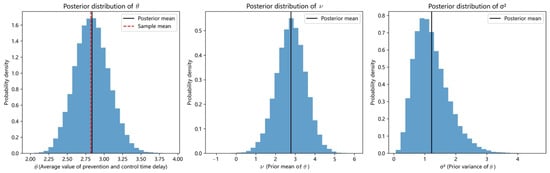
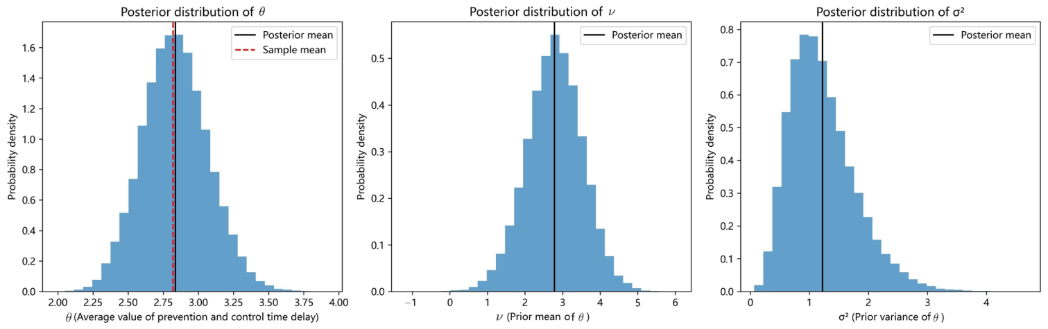
Posterior distributions. Figure 5 displays the posterior densities and trace plots for $\theta$, $\nu$, and ${\sigma }^2$. The posterior summaries are provided in Table 3.

Figure 5. Posterior distributions of hierarchical Bayesian model parameters (based on actual data).

Table 3. Posterior inference of model parameters.

Parameter	Posterior Mean	95% Credible Interval
$\theta$	2.8349	[2.3918, 3.3083]
$\nu$	2.7945	[1.2827, 4.2601]
${\sigma }^2$	1.2442	[0.3913, 2.5959]

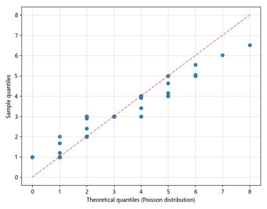
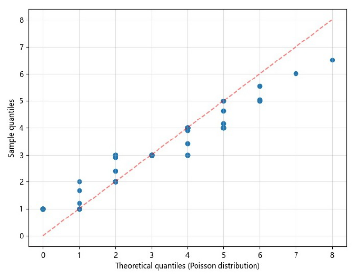
Model evaluation. Figure 6 presents the Q–Q plot comparing model-predicted quantiles with observed data quantiles. The points lie approximately along the 45° reference line, indicating that the model captures the overall data distribution well.

Figure 6. Q-Q Plot: Model predictions vs. actual data).

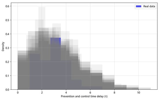
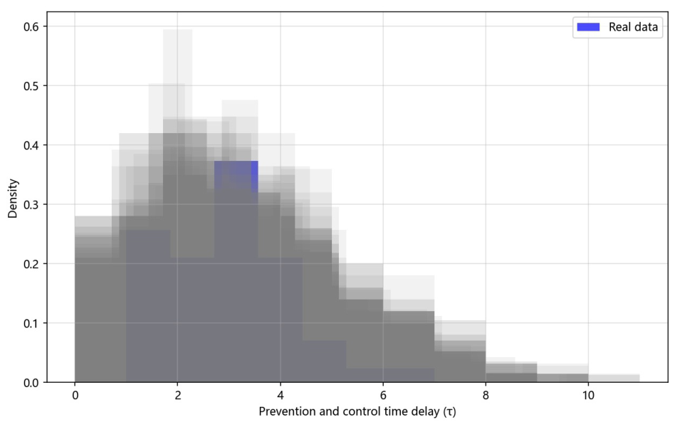
Figure 7 shows the posterior predictive check (PPC), where the observed data density (blue line) falls entirely within the gray shaded region representing 300 simulated predictive densities. This confirms that the model adequately reproduces both the central tendency and the tail behavior of the observed data.

Figure 7. Posterior predictive check (PPC).

5.5. Practical Significance and Integration with Bifurcation Analysis

The time-delay SEIR model is conceptually independent of the hierarchical Bayesian model, as the two frameworks differ fundamentally in their construction. Nevertheless, the parameter values employed in both the theoretical and numerical analysis (e.g., $a=0.22$, $b=0.3667$, $d=0.005$, $g=0.0265$, $\delta =0.01$, $\mu =0.6$) are derived from statistical data and should be reasonably consistent with the posterior estimates obtained from the Bayesian procedure, as both modeling frameworks draw upon data originating from the same underlying biological system and share the same empirical context. Consequently, we posit that the two modeling strategies mutually validate one another, offering convergent evidence for our conclusions.

From the hierarchical Bayesian inference, the posterior mean of the mean delay $\theta$ is $2.8349$ days, with a $95\%$ credible interval $[2.3918,3.3083]$. As shown in Section 4, the critical delay for the Hopf bifurcation is ${\tau }_0\approx 3.5279$ days.

• If $\tau <{\tau }_0$, the disease persists at a stable endemic equilibrium.
• If $\tau >{\tau }_0$, periodic outbreaks may emerge.

The estimated delay $\theta$ (interpreted as the expected value of $\tau$) lies consistently below ${\tau }_0$; notably, the upper bound of the $95\%$ credible interval ($3.3083$) remains below $3.5279$. We therefore conclude that, under current prevention and control practices in this region, periodic outbreaks are unlikely to occur. Timely detection and intervention keep the delay below the bifurcation threshold.

The basic reproduction number $R_0$, being independent of $\tau$, is evaluated with the parameter values given above as follows:

$$R_0={\displaystyle \frac{ag}{d(b+d)}}\approx 3.1372>1,$$

indicating that the disease remains endemic even though periodic outbreaks are avoided.

These findings offer a quantitative foundation for designing prevention and control strategies, which we detail below in connection with field management.

• Critical delay ${\tau }_0$ as a timeliness threshold. The value ${\tau }_0=3.5279$ days defines a quantitative timeliness standard: to avoid periodic outbreaks, growers should complete the removal or chemical treatment of diseased plants within $3.5$ days after detection.
• Bayesian inference of $\tau$ as a practical reference. The posterior mean of $\tau$ ($2.83$ days; $95\%$ credible interval $[2.39,3.31]$) confirms that the actual control lag in the field is less than ${\tau }_0$, validating the timeliness of current measures. This also provides a benchmark for adjusting control frequency across different regions.
• Basic reproduction number $R_0$ as a transmission potential index. $R_0>1$ reveals a strong transmission potential of sugarcane PB in the field. Specific measures to reduce $R_0$ include increasing the removal rate $\mu$ and lowering planting density to reduce the infection rate a.
• Hopf bifurcation as an early warning signal. The bifurcation diagram can serve as an early warning tool: if the actual control lag approaches ${\tau }_0$, growers should strengthen control measures preemptively.

Collectively, these results substantiate the claim that our model provides a comprehensive and effective theoretical basis for decision-making in the prevention and control of sugarcane PB, bridging theoretical analysis with actionable field management.

6. Conclusions and Discussion

We have developed a time-delay SEIR model for sugarcane PB, demonstrating that Hopf bifurcations occur when the time delay $\tau$ crosses a critical value. Subsequently, we applied a hierarchical Bayesian framework to perform statistical inference on $\tau$, complemented by convergence diagnostics and model evaluation. Together, these results furnish a comprehensive theoretical basis for decision-making in the prevention and control of sugarcane PB.

6.1. Biological Justification of the Conclusions

Each key conclusion is directly linked to the biological characteristics of sugarcane and PB:

• The contrast between asymptotic stability ($\tau <{\tau }_0$) and periodic outbreaks ($\tau >{\tau }_0$) aligns with the observed seasonal variation of PB incidence in the field, where delays in manual control often trigger recurrent epidemics.
• The long growth cycle of sugarcane and the airborne transmission pathway of PB make timely intervention critical; hence, the time delay $\tau$ plays a decisive role in disease dynamics.
• The estimated $R_0\approx 3.1372$ reflects a high transmission potential under current agronomic practices, underscoring the need for integrated management strategies.

6.2. Comparison with Existing Models

To our knowledge, no existing SEIR or time-delay mathematical model has been specifically developed for sugarcane PB. We therefore compare our model with related plant disease models that share similar epidemiological features (e.g., airborne fungal pathogens, perennial host crops), including models for rice blast [21], wheat rust [3], and other sugarcane diseases such as smut and mosaic [11].

Our model differs from these existing models in three fundamental aspects:

1.

Targeted introduction of time delay for control measures. Existing plant disease models usually either ignore time delays or incorporate them for other biological processes (e.g., latency period). By introducing $\tau$ specifically to represent the lag in control measure implementation (e.g., removal or chemical treatment), our model captures a critical but often overlooked aspect of field management.

2.

Integration of dynamic analysis and statistical inference. Most plant disease models with time delay restrict themselves to dynamic analysis. In contrast, our work combines Hopf bifurcation analysis with hierarchical Bayesian inference, thereby unifying theoretical exploration and empirical validation.

3.

Quantitative guidance for control. Previous studies on plant disease control often provide only qualitative recommendations. Our model yields quantitative control thresholds (e.g., when $\mu =0.6$, ${\tau }_0<3.53$ days), which offer more direct and actionable guidance for field management.

Given the absence of prior SEIR modeling for PB, this study represents the first effort to (i) establish a time-delay SEIR framework specifically for this disease, (ii) conduct Hopf bifurcation analysis for PB dynamics, and (iii) combine dynamic analysis with hierarchical Bayesian inference for parameter estimation.

6.3. Limitations and Future Work

Although the proposed time-delay SEIR model provides a meaningful description of disease dynamics, opportunities for improvement remain in both the structural realism of the differential equation framework and the statistical inference of key parameters.

6.3.1. Limitations of the Current Study

For instance, the relatively small sample size ($n=50$) imposes weak constraints on the hyperparameters $\nu$ and ${\sigma }^2$, leading to wide $95\%$ credible intervals. Additionally, the current model assumes homogeneous farmer behavior and constant environmental conditions, which may not fully capture the variability observed in real-world field settings. Environmental factors such as temperature, humidity, and seasonal variations can influence pathogen transmission and disease progression, while heterogeneity in farmer behavior—including differences in detection speed, compliance with control measures, and resource availability—can significantly affect the actual control lag $\tau$.

6.3.2. Future Research Directions

To address these limitations and enhance the model’s practical relevance, future research should focus on the following directions:

• Expand data dimensions. Increase the number of observational samples or incorporate multi-source data (e.g., regional and policy covariates) to improve the estimation accuracy of higher-level parameters. Larger-scale and multi-regional field datasets are needed to further validate the model’s robustness and generalizability, as highlighted by the reviewer.
• Optimize prior structure. Adjust ${\nu }_0$ and ${\sigma }_0^2$ based on domain knowledge—for example, by reducing the prior variance to strengthen constraints—or adopt alternative weakly informative priors for ${\sigma }^2$ to mitigate the impact of skewness on posterior inference.
• Extend model settings with random effects. Introduce random effects to capture individual heterogeneity (e.g., variation in detection speed or compliance across different farmers or regions), thereby enhancing the model’s ability to fit complex data.
• Incorporate environmental and behavioral covariates. Explicitly link environmental variability (e.g., temperature, humidity, seasonal indices) to key model parameters such as the infection rate a and the removal rate $\mu$. Similarly, link farmer behavior heterogeneity (e.g., differences in response time, adherence to control protocols) to the time delay $\tau$. This can be achieved through hierarchical modeling approaches that include region-specific or farm-specific covariates, or through the development of sub-models that describe how environmental and behavioral factors modulate transmission and control dynamics.

These extensions will strengthen the model’s practical relevance for field management across different regions and farming systems, providing a more realistic and actionable tool for sugarcane PB prevention and control.

References

- FAOSTAT. Sugarcane: Area Harvested and Production. The Food and Agriculture Organization of the United Nations. 2025. Available online: https://www.fao.org/faostat/en/#data/QC (accessed on 1 January 2020).
- FAOSTAT. Crops: Sugarcane. The Food and Agriculture Organization of the United Nations. 2021. Available online: https://www.fao.org/faostat/en/#data/QC (accessed on 28 July 2021).
- Tiwari, R.; Shukla, S.K.; Jaiswal, V.P.; Tiwari, R.K. Pokkah boeng disease of sugarcane: Current status and opportunities. Curr. Adv. Agr. Sci. 2020, 12, 1–6. [Google Scholar] [CrossRef] [Scilit]
- Viswanathan, R.; Sundar, A.R.; Malathi, P. Omics applications to decipher host-pathogen interactions and to understand pathogens in sugarcane. In Omics Approaches for Sugarcane Crop Improvement; CRC Press: Boca Raton, FL, USA, 2022; pp. 99–130. [Google Scholar] [CrossRef] [Scilit]
- Yonzone, R.; Devi, M.S. Red stripe/top rot disease of sugarcane: A review. Int. J. Curr. Microbiol. Appl. Sci. 2018, 7, 1469–1478. [Google Scholar] [CrossRef] [Scilit]
- Siva, M.; Sendhilvel, V.; Thangeswari, S. Etiology and histopathological insights of Twisted top disease: A re-emerging threat to sugarcane cultivation. Physiol. Mol. Plant Pathol. 2025, 139, 102747. [Google Scholar] [CrossRef] [Scilit]
- Martin, J.; Handojo, H.; Wismer, C. Pokkah boeng. In Diseases of Sugarcane: Major Diseases; Elsevier: Amsterdam, The Netherlands, 1989; pp. 157–168. [Google Scholar] [CrossRef] [Scilit]
- Raid, R.N.; Lentini, R.S. Pokkah Boeng Disease of Sugarcane; Institute of Food and Agricultural Sciences, University of Florida Cooperative Extension Service: Gainesville, FL, USA, 2002. [Google Scholar]
- Siti, N.; Mohamed, S. Pathogenicity and Aethiology of Fusarium species Associated with Pokkah Boeng Disease on Sugarcane; Universiti Sains Malaysia: George Town, Malaysia, 2007. [Google Scholar]
- Lin, Z.; Zhang, Y.; Que, Y.; Chen, R.; Chen, B.; Zhang, M. Characterization of Fusarium verticillioide isolates from pokkah boeng on sugarcane and the disease incidence in field. J. Microbiol. Exp. 2015, 2, 1–7. [Google Scholar] [CrossRef] [Scilit]
- Viswanathan, R.; Balaji, C.G.; Selvakumar, R.; Malathi, P.; Sundar, A.R.; Prasanth, C.N.; Chhabra, M.L.; Parameswari, B. Epidemiology of Fusarium diseases in sugarcane: A new discovery of same Fusarium sacchari causing two distinct diseases, wilt and pokkah boeng. Sugar Tech. 2017, 19, 638–646. [Google Scholar] [CrossRef] [Scilit]
- Viswanathan, R.; Geetha, N.; Salin, K.P.; Selvakumar, R.; Malathi, P.; Sundar, A.R.; Nithyanantham, R.; Manivannan, K. Twisted top disease a destructive disease of sugarcane in India. Indian Phytopathol. 2023, 76, 625–630. [Google Scholar] [CrossRef] [Scilit]
- Wang, C.; Yin, J.; Li, Y.; Li, J.; Zhang, R.; Wang, X.; Shan, H.; Luo, Z. Multi-gene identification and pathogenicity analysis of sugarcane pokkah boeng in Yunnan, China. Trop. Plant Biol. 2024, 17, 296–305. [Google Scholar] [CrossRef] [Scilit]
- Kermack, W.O.; McKendrick, A.G. A contribution to the mathematical theory of epidemics. Philos. Trans. R. Soc. Lond. Ser. A 1927, 115, 700–721. [Google Scholar] [CrossRef] [Scilit]
- Hethcote, H.W. The mathematics of infectious diseases. SIAM Rev. 2000, 42, 599–653. [Google Scholar] [CrossRef] [Scilit]
- Anderson, R.M.; May, R.M. Infectious Diseases of Humans: Dynamics and Control; Oxford University Press: Oxford, UK, 1991. [Google Scholar] [CrossRef] [Scilit]
- Zhang, D.; Britton, T. An SEIR network epidemic model with manual and digital contact tracing allowing delays. Math. Biosci. 2024, 374, 109231. [Google Scholar] [CrossRef] [Scilit] [PubMed]
- Barman, M.; Mishra, N. Hopf bifurcation analysis for a delayed nonlinear-SEIR epidemic model on networks. Chaos Solitons Fractals 2024, 178, 114351. [Google Scholar] [CrossRef] [Scilit]
- Moumine, E.M.; Khassal, S.; Balatif, O.; Rachik, M. Modeling and analysis of a fractional order spatio-temporal SEIR model: Stability and prediction. Results Control Optim. 2024, 15, 100433. [Google Scholar] [CrossRef] [Scilit]
- O’Hara, R.B.; Sillanpaa, M.J. A review of Bayesian variable selection methods: What, how and which. Bayesian Anal. 2009, 4, 85–118. [Google Scholar] [CrossRef] [Scilit]
- Adrakey, H.K.; Gibson, G.J.; Eveillard, S.; Malembic-Maher, S.; Fabre, F. Bayesian inference for spatio-temporal stochastic transmission of plant disease in the presence of roguing: A case study to characterise the dispersal of Flavescence dorée. PLoS Comput. Biol. 2023, 19, e1011399. [Google Scholar] [CrossRef] [Scilit] [PubMed]
- Kuang, Y. Delay Differential Equations with Applications in Population Dynamics; Academic Press: Cambridge, MA, USA, 1993. [Google Scholar]
Disclaimer/Publisher’s Note: The statements, opinions and data contained in all publications are solely those of the individual author(s) and contributor(s) and not of MDPI and/or the editor(s). MDPI and/or the editor(s) disclaim responsibility for any injury to people or property resulting from any ideas, methods, instructions or products referred to in the content. |
© 2026 by the authors. Licensee MDPI, Basel, Switzerland. This article is an open access article distributed under the terms and conditions of the Creative Commons Attribution (CC BY) license.