


Abstract
In this study, we propose a general mathematical modelling framework based on the characteristics of elite athletes’ movements in the touch rugby matches to investigate the dynamic relationship between physical workload and injury risk over time. Our framework extends the Cox-based model in the context of touch rugby by incorporating a time-scaling component and cluster-specific heterogeneity simultaneously. In addition, we allow for the inclusion of covariates (e.g., velocity variation) to capture their effects. We applied our model to high-frequency wearable sensor data collected from 27 elite athletes (15 men and 12 women). The empirical study results show that our model, time-scaled frailty model (TSFM), demonstrates better goodness-of-fit than traditional frailty and Andersen–Gill models. The results reveal that higher velocity variation, particularly during high-intensity phases, and longer time of continuous exposure to the workload spike state significantly increased overload risk, ultimately resulting in injury. It also highlights the importance of individual differences, even under the same exercise intensity. These insights provide coaches with an evidence-based framework for athlete monitoring, allowing for more personalized training loads, tactical deployment, and injury prevention strategies in elite touch rugby environments.
Keywords:
survival analysis; frailty model; recurrent events modelling; unobserved heterogeneity; external workload analysis; piecewise exponential additive mixed model MSC:
62H12; 62J12; 62N02; 62P10
1. Introduction
Touch rugby is a fast-paced and intermittent team sport that combines high intensity movement with frequent transitions between offence and defence. Unlike traditional rugby, strong physical tackle is replaced by light hand touch, focusing on agility and sprinting. Matches are typically played on a 70 m × 50 m field with six athletes per team, which allows unlimited substitutions throughout the match that are two 20 min halves [1]. Despite the removal of strong physical tackles in touch rugby, which contributes to a lower injury incidence, the sport still imposes substantial physical demands, including intermittent high-intensity efforts and rapid accelerations. Consequently, athletes experience an elevated risk of sustaining injuries, particularly to the ankle and knee joints [2]. In addition, different playing positions involve distinct physical demands and movement intensities, leading to varying levels of injury risk [3]. Thus, analysing and comparing the movement patterns of touch rugby athlete across different clusters, with each cluster categorized by shared kinematic features, can help identify high-risk movements, inform workload management, and support the development of effective injury prevention strategies.
Recent research has shown that wearable technology plays an increasingly important role in monitoring and tracking athletes’ movements, as well as collecting these data, during training and matches, which are subsequently used to improve training and optimize match strategies effectively [4,5,6]. The advancement of wearable tracking systems, including GPS and inertial sensors, can enable more comprehensive analysis of athletes’ workloads. Therefore, these systems have become widely adopted in the field of sport science to help mitigate injury risk and optimize match strategies [7]. In particular, the metrics obtained from these wearable tracking systems, including distance, velocity, and other related measurements, can be used to estimate the internal and external workloads of athletes [8,9,10,11]. So, it can help coaches understand how hard athletes work, adjust training plans, and set up a reasonable recovery plan. For example, Beaven et al. employ GPS data to quantify physical demand by capturing the velocity of elite male athletes, and identify how frequently athletes transition between different intensity levels [12]. In addition, devices with embedded GPS technology have been widely used to capture athlete movement profiles in various team sports, such as football, rugby, etc. [13,14]. These data have been used to measure athletes’ activities and analyse their work rate patterns during matches and training, allowing coaches to better understand the physical condition of each member of the team and develop a data driven match strategy [13].
Although GPS technology has been widely used in court-base sports, its reliability has raised concerns and been discussed in the recent literature. Jennings et al. show that GPS with a higher frequent sampling rate is more reliable and precise in measuring distance [15]. In contrast, the GPS device with a frequency of 1 Hz has been verified to not accurately capture movement data, which takes less than 1 s [4]. The more recent GPS device with 10 Hz allows us to measure small changes in velocity changes with a good accuracy level [16,17]. The reliability of a 10 Hz GPS unit for monitoring quick acceleration and deceleration has been further validated by Nikolaidis et al. [18].
Undoubtedly, with the rapid development of technology, especially in wearable sensors (GPS), athlete performance analysis has entered a new era in touch rugby. The availability of GPS data with detailed information allows researchers and coaches to go beyond simple summaries, by using statistical and mathematical models. For example, Beaven et al., Chow, Vickery and Harkness employed descriptive statistics and basic statistical tests, such as t-tests and ANOVA, on GPS data, to assess differences between playing positions [12,19,20]. They found that wings generally covered greater distances while middles had higher intensity metrics. Moreover, Vickery and Harkness used GPS data collected from national touch tournaments to investigate mixed gender competitions, focusing on differences in workload intensity between genders, and provide a suggestion on adjustments in training programs [20]. Zaragoza et al. provided further analysis on gender-specific workload demands at the international level, emphasizing the essential nature of individualized training thresholds for male and female athletes [21].
Although these studies provided valuable insights on workload demand, they fail to capture the characteristics in the dynamics of athletes’ movements and do not adequately identify underlying cause-and-effect relationships associated with injury-related risk. More specifically, there is a lack of existing research that rigorously examines the relationship between kinematic-derived movement patterns and injury-related risk in touch rugby matches. Therefore, in this study, we analyse the movement dynamics of each player by using high-frequency velocity and acceleration data, to better understand and characterize their underlying mechanisms and behavioural features for the different clusters. Then, based on our observation, we move beyond the descriptive statistical analysis and employ a survival analysis technique to determine the relationship between movement characteristics and the injury-related risk, as survival analysis can model the recurrent events, estimate the instantaneous risk of such events at any given time points, and incorporate multiple predictors to assess their effects on the risks. Moreover, the existing models within the court-based sports have limitations, as they fail to capture time-scaling dynamics and cluster heterogeneity simultaneously [22]. To address this issue, we integrate the time-scale components into the shared frailty framework in this study.
The remaining structure of the paper is organized as follows: Section 2 synthesizes the extant literature on workload–injury analysis and modelling approaches. Section 3 develops a novel and comprehensive framework for modelling workload–injury in touch-rugby. Section 4 describes and analyses the tough rugby data collected from New Zealand matches. Section 5 shows the results of our models and discusses the key findings of the results. Section 6 concludes.
2. Related Work
Research examining the triadic relationship between load, fatigue, and injury risk demonstrates that external workload acts as a driver of fatigue accumulation and subsequent injury [23,24,25,26]. Several metrics, such as acute chronic workload ratio (ACWR), session rating of perceived exertion (sRPE), distance, high-speed running, etc., have been developed to assess this relationship [13,25,27,28]. The external workload metrics obtained via wearable devices quantify the physical work performed by an athlete. In other words, these metrics include, for example, high-speed running distance, velocity, and so on. However, they do not directly capture athletes’ fatigue levels or provide meaningful insights into injury risk based solely on their values [29,30]. Unlike standard workload metrics, ACWR integrates recent and historical information, so it can offer an individualized measure of physical demands and refine injury risk assessment [25]. Consistent with the workload–injury nexus, Hulin et al. revealed that an ACWR value greater than 1.5 indicates a workload spike and is associated with a greater probability of injury occurrence [28].
Although these studies offered pivotal findings within the workload–injury nexus, they provided limited mechanistic insight into understanding the interplay between injury and the temporal dynamics of athlete fatigue levels. To address this problem, recent research in this area has shifted the focus to more sophisticated statistical frameworks, most notably survival analysis. This approach models the instantaneous hazard of injury through time-to-event analysis, serving as a powerful tool for risk assessment in sports science [22]. They also emphasized that survival analysis techniques are well-suited to explore fundamental questions, including how workload influences injury risk over time, how multiple injuries accumulate, and how to deal with competing risks in injury data [22].
In the early years, researchers provided a non-parametric way to estimate survival curves from censored data [31]. In 1972, Mantel introduced the log-rank test and provided a formal statistical method to compare survival curves among groups, allowing researchers to test whether differences in time-to-injury trajectories, such as injury incidence patterns across distinct workload quartiles or athlete positions [32]. During the same year, a landmark model in the field of survival analysis is the proportional hazards model introduced by Cox. He proposed a hazard function, allowing covariates to have a multiplicative effect on the baseline hazard, that is,
where denotes p covariate values; is the vector of unknown parameters; is the hazard failure rate at failure time T,
and is the unknown hazard function that is defined under the condition = 0 [33].
The Cox model has quickly become the dominant tool for analysing time-to-event outcomes due to their robustness, methodological flexibility, and interpretability. For example, Gabbe et al. used a Cox regression to identify risk factors by adopting a time-to-event approach that centres on the time to the first hamstring strain, which is the accumulation of on-field exposure hours prior to the event, in community Australian football [34]. It demonstrated the imperative of incorporating a temporal dimension into the model in injury analysis. In addition, researchers utilized other approaches, such as the Kaplan–Meier estimator, the exponential survival model, the Weibull survival model, etc., to study the time-to-first-event from different aspects, including survival probability and covariate effects [22,35,36]. These methods allow for the investigation of injury timing and athlete-specific risk, offering a more comprehensive approach to injury prediction and workload management [37]. The majority of survival models are centred on modelling the duration of event-free participation prior to the first failure event; however, limited empirical attention has been directed toward the modelling of recurrent events in the sport science area [37,38]. Matches and training sessions frequently involve some recurrent events, such as high-intensity movements and injury; therefore, it is important to extend the models to accommodate recurrent events.
To address recurrent events, statisticians introduced the Andersen–Gill (AG) model, which extends Cox’s proportional hazards model by treating each recurrence as a new “starting point” [39]. In the AG model, it is assumed that, under given covariate information, each event is independent and identically distributed, with a shared baseline hazard for all recurrences, so it can explicitly capture the changes in risk probability for subsequent events [40]. Another key assumption of this model is that all event times are also conditionally independent of the given covariates. These assumptions imply that the risks of the recurrent event are identical to those of the first event when all other covariates remain unchanged. When implemented in a sporting context, these assumptions may be unrealistic. For example, Venturelli et al. found that the prior injury significantly elevated the hazard ratio for subsequent re-injury [41]. The Prentice–Williams–Peterson (PWP) model, an extension of Cox’s proportional hazards model, can be applied to address this issue. The PWP model considers the order of recurrent events and accounts for the possibility that the baseline hazard of the subsequent event could be higher than that of the previous event [42]. Furthermore, literature identifies several sophisticated extensions for modelling recurrent events, including Wei, Lin, Weissfeld model (WLW) (Wei, Lin, and Weissfeld model (WLW) is another extension of Cox proportional hazards model. In contrast to the AG model, it does not require each recurrence event to have the same baseline hazard), and shared frailty Cox model. The Cox shared frailty model was applied to analyse injury data from an Australian rugby league season, and the empirical evidence presented in this study further supports that previous injuries, regardless of the type of injury, substantially affect the risk of future injury [43].
Although the above extensions, such as accounting for recurrent events and event ordering, have enhanced analytical approaches in survival analysis, the field has progressed toward the inclusion of unobserved heterogeneity among individuals. It is widely recognized that the physiological status or functional capacity of an individual athlete can exhibit significant variance; however, these factors cannot be directly and easily measured by devices. Therefore, the term “frailty” was introduced into the survival analysis to account for this issue. Frailty is modelled as a random latent variable, capturing unobservable individual characteristics. Consequently, it affects the hazard rates in the analysis [44]. Incorporating frailty (a random effect) in the model can flexibly capture the inherent heterogeneity of individual profiles [45]. In most models, the unobserved individual-level frailties are assumed to follow gamma or normal distributions [46,47]. For example, Macis applied the frailty model to evaluate the risk factors of injury [48]. He found that the Cox regression model with frailty can provide a better explanation of the injury data of NBA athletes and emphasized that individual factors can influence the baseline risk of injury [48].
3. The Workload–Injury Model
In this section, we propose a general framework for workload–injury modelling within the context of elite touch rugby athletes, which can be applied to other disciplines in the sports science areas. It demonstrates how survival analysis can be employed to model the risks of injury or injury-related events as a function of influencing factors.
3.1. Workload Spike State
As we know, in touch rugby, athletes are repeatedly exposed to rapid accelerations, decelerations, and frequent changes of direction, which can cause frequent and sudden increases in external workload, thereby increasing the probability of injury [49]. Based on these characteristics, the Acute Chronic Workload Ratio (ACWR) is a good choice to identify the workload spike in touch rugby matches. According to Hulin et al., using metabolic power in the calculation of ACWR can easily detect sudden changes in external workload and provide a robust measurement of risk over short periods based on every person’s physical fitness [28]. The metabolic power is an approach that can accurately quantify the instantaneous external workload in matches. In this paper, we adopt the di Prampero et al.’s method to calculate the metabolic power. In this framework, both velocity and acceleration are used to calculate [8]. For detailed calculation processes, see the Appendix A.
Following Hulin et al., the ACWR can be calculated as
where acute workload is short-term load, which usually refers to the most recent workload (e.g., past 1 week); chronic workload refers to the average workload over a longer preceding period (e.g., past 4 weeks) [28]. The ACWR can detect the short-term fluctuations in workload in relation to relatively longer-term adaptation. Hulin et al. observe that an ACWR exceeding 1.5 indicates a significant increase in the risk of injury [28]. So, we consider an ACWR that exceeds 1.5 for an athlete as a workload spike event, and the threshold in (2) can be set as 1.5 or higher. Furthermore, Hulin et al. state that the high ACWR value is associated with an increased injury risk for the subsequent period [28]. Thus, entry into the workload spike state is associated with an increased likelihood of injury in the subsequent match period.
3.2. The Model
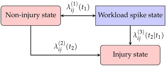
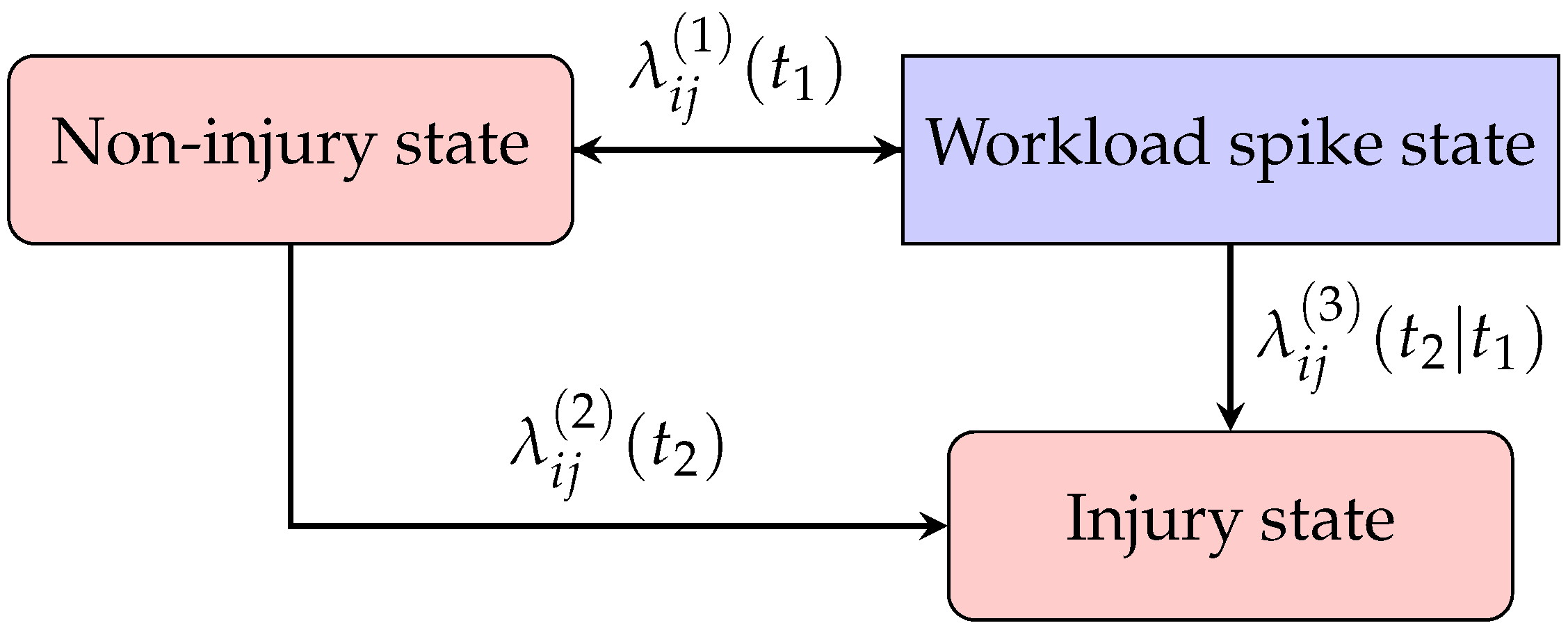
In our general model framework, three states—non-injury, workload spike, and injury states—are considered. The workload spike state has been defined in Section 3.1. The transitions between these states are illustrated in Figure 1. We assume that the workload spike event repeatedly occurs for each athlete during match periods, and once an athlete is injured, he or she does not return to the match. Thus, the workload spike event and injury event can be treated as non-terminal and terminal events, respectively.
Figure 1.
Risk setting in touch rugby match.
To further generalize our model, we account for clustering effects and introduce cluster-specific frailty into the model for unobserved heterogeneity between the clusters. Suppose that n athletes can be classified into m clusters based on the shared characteristics within the cluster. Let denote the end time of the match and denote the time to the injury event for ith athlete. If no injury occurred during the match for the athlete i, then is censored at the end of the match, otherwise . For the workload spike event, we have n-counting processes adapted to a filtration , where counts workload spike events for athlete i, during the match period, which are step functions, zero at the start time of the match with jump size 1, such that
where is the time of the kth spike in the workload event.
Similarly, we also have n-counting processes for the injury event, which is
Now, we assume that and have random intensities, and , where j denotes the cluster to which the athlete i belongs. Let and be indicator functions of the athlete i who experiences a spike in workload and is injured at time t (), such that
where a detailed calculation of the workload spike state index is provided in Section 3.1, and
Inspired by the works of Anderson and Gill [40], Xu et al. [50], and Keiding et al. [51], we assume that covariates simultaneously affect both the time and hazard scales. So, the general framework for modelling transition rates (hazard rates) illustrated in Figure 1 is expressed as follows.
and
where represents the transition rate from a workload spike to injury; equals 1 if the athlete i is injured after experiencing a spike in workload, otherwise 0; is a vector of time-dependent covariates, representing factors that contribute to increasing the risk of the athlete i being injured; , , represent the baselines of their corresponding hazard rate functions; and , , , and , for , are regression coefficients. Furthermore, , and are frailty terms for the cluster j and are assumed to be time-independent. We adopt a normal distribution for the frailty term, , for . This choice is motivated by Gabbett et al., which suggest that athlete-specific unobserved effects, such as physiological factors, are typically continuous in nature and tend to be symmetrically distributed around a population mean [52]. In addition, there is no correlation between frailty terms. It represents an unobserved random effect that captures group-level heterogeneity, as different groups may exhibit distinct movement patterns and therefore affect levels of injury risk. It is also time-independent and shared between all members within the cluster. Moreover, for simplicity, we assume no correlation between clusters and that the frailty terms are independent of the covariates. However, we acknowledge that some correlation may exist. If this assumption is violated, the results may be biased and misleading. Hence, the alternative methods that allow for correlated frailty terms may be more appropriate, but we leave this for future research.
To estimate the parameters of our proposed framework in Equations (4)–(6), we employ the joint calibration method of the Piecewise Exponential Additive Mixed Model (PAMM) framework and the L-BFGS-B optimization algorithm based on the Restricted Maximum Likelihood (REML) objective function and AIC values. The PAMM framework is particularly effective and well-suited for our case. There are two main reasons. First, unlike Cox-type models with frailty, which assume constant covariate effects over time, PAMM provides a flexible method that accommodates non-linear time-varying covariate effects and random effects without requiring the strict proportional hazards assumption [53]. Second, because our data are high-frequency, PAMM can provide more efficient computation than using “frailtypack” in R, as the maximum penalized likelihood estimation procedure in “frailtypack” can be very time-consuming for large datasets.
In the joint calibration method, we approximate the hazard function in the PAMM framework. More specifically, this method divides the observation period into small intervals, allowing the model to incorporate covariates that vary over time, such as changes in velocity over time [53]. This is a smart and fast algorithm that works well even when we need to set limits (or boundaries) on the parameters [53,54].
3.3. The Application in New Zealand Touch Rugby Data
Multiple workload spike events are identified for each athlete from the New Zealand touch rugby match dataset; however, no injury events were recorded for any athlete throughout the period. This may be because athletes spend the majority of their time in relatively low-intensity phases, with only occasional periods of very high-intensity activities. For more detailed information on the characteristics of touch rugby, refer to Section 4. Since no injuries were observed, we derive a simplified version of the model presented in Section 3.2. That means this model only considers the transition rate from the non-injury state to the workload spike state. Moreover, we consider two covariates in this study, motivated by the dynamic nature of touch rugby, which involves frequent transitions between different velocity levels. The first one is the velocity variation over the 30 s window ending 3 s before the current time t, denoted as , as this factor reflects fluctuations in movement intensity, and it has been associated with injury risk in the work of Cropper et al. [2]. The second one is the continuous time exposure to the spike state, recorded 10 s before the current moment, denoted as . Moreover, this variable measures the length of interrupted time when the velocity is greater than a predefined threshold. Due to the lack of historical data, the thresholds are used 3 m/s for female and 3.5 m/s for male in this study based on Sweeting et al. [55]. We include this covariate because it reflects how fatigue accumulates over time.
Next, we discuss how the event is defined. Due to the limited data coverage (only two matches) and the nature of touch rugby, which involves short bursts of high-intensity activity, the conventional weekly ACWR windows are not appropriate. Instead, a shorter time window (30 s window) is selected as the short-term measure, because it is sensitive to local variability and sudden changes while avoiding overreaction to transient fluctuations. In line with the conventional ACWR framework, a 4:1 ratio between long-term and short-term windows is adopted, as it can provide a more balanced comparison and enables reliable identification of rapid changes relative to the recent context. Therefore, we defined ACWR by following (1) as
where represents acute workload at time t, derived from the average metabolic power over the preceding 30 s, including the current time point, and represents chronic load at time t, derived from the average metabolic power over the preceding 120 s, including the current time point. This ratio captures how much the current short-term workload exceeds the recent baseline and a sudden increase in physical demand. Compared with the conventional ACWR, this ratio is better suited for analysing acute intensity patterns, particularly in situations where intensity fluctuates rapidly. We define a workload spike event when the value of is greater than . Thus,
Based on our proposed framework in this section and the availability of data, the hazard function in this example simplifies to a one-dimensional function, given by
where and are the coefficients of ; and are the coefficients of ; and . Hereafter, we refer to this model (8) as the time-scaled frailty model (TSFM).
To evaluate the feature significance, we compare the full version model (8) with the simplest version where specific features are removed. A decrease in performance suggests that the removed features are critical to the model’s predictive power. Therefore, we first propose a reduced model of our full model that excludes a time-scaled feature, allowing us to isolate the impact of the time-scaled feature. In the following, we refer to this model as the FM model. Then, to evaluate the contribution of cluster-specific frailty, we also proposed further degenerate models that exclude the cluster-specific frailty term and are derived from the well-established Andersen–Gill model, so we refer to this model as the AGM model. Finally, we exclude covariance terms from the FM and AGM models to evaluate the impact of covariance. We refer to these two models as BFM and BAGM, respectively.
4. Data
In this section, we explore the data from New Zealand touch rugby matches, including male and female matches, apply our general framework to this data set, and investigate how the athletes’ movement patterns during matches influence the probability of injury.
The data used for this study consist of high-frequency information collected during touch rugby matches in New Zealand, involving 27 national-level athletes (15 male, 12 female). The data were collected using GPS devices during matches in which athletes competed against the opposing teams. The dataset includes two full-match observations for each player within the same season. However, data corresponding to halftime periods were excluded from the analysis. It records the velocity, acceleration, and distance at 0.1 s intervals for each athlete during matches, using GPS sensors that operate at a rate of 10-Hz. In this section, we will perform statistical analysis and obtain a deep understanding of each individual’s profile.
4.1. Exploratory Data Analysis
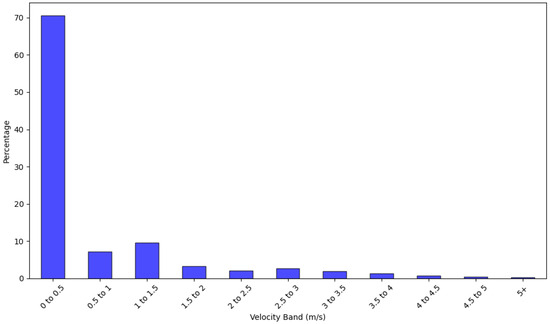
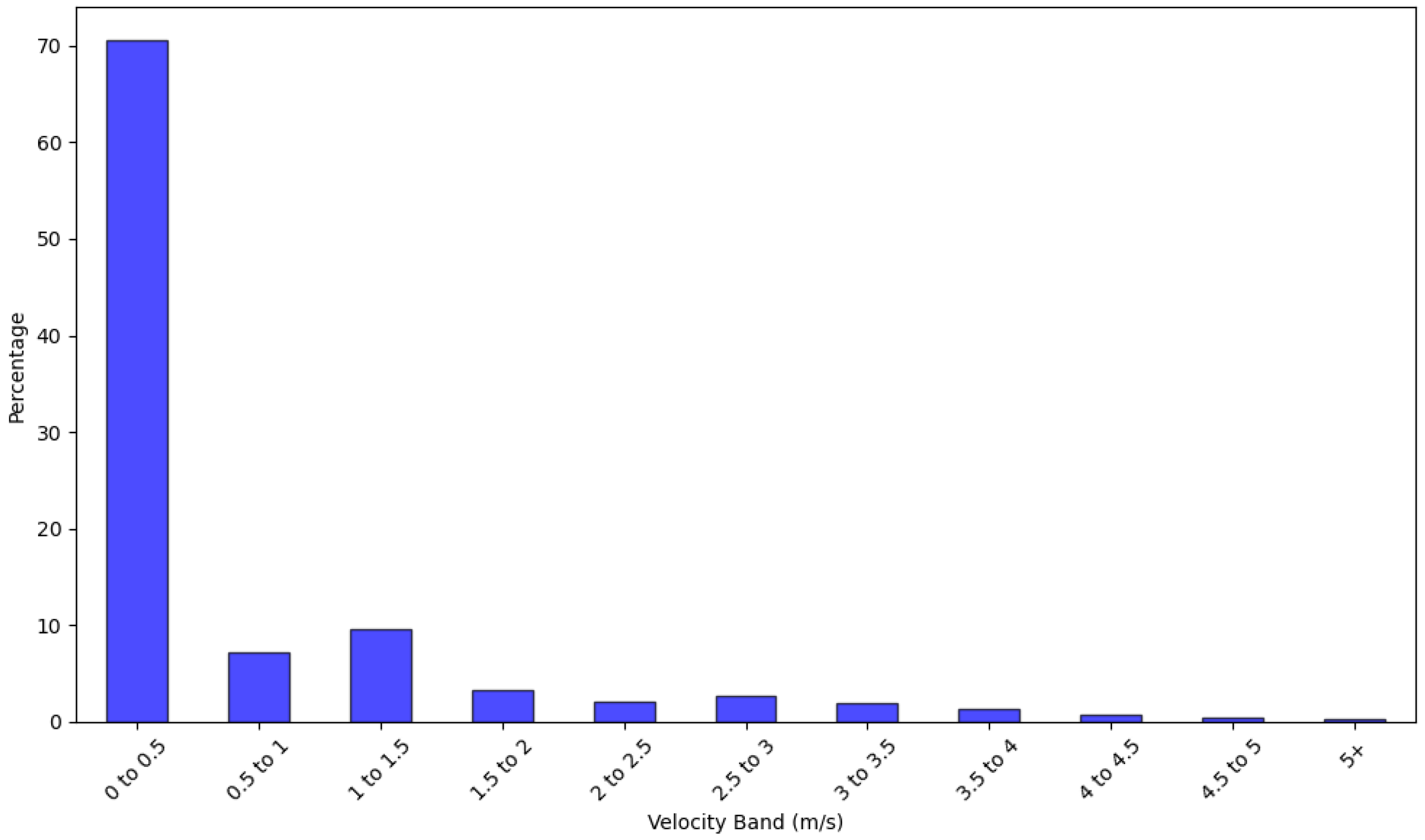
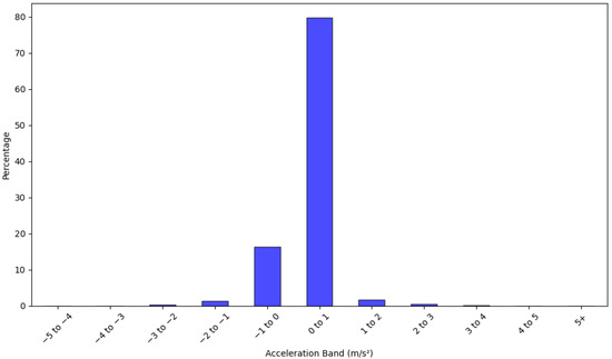
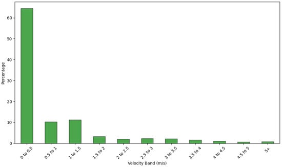
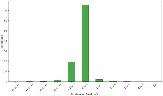
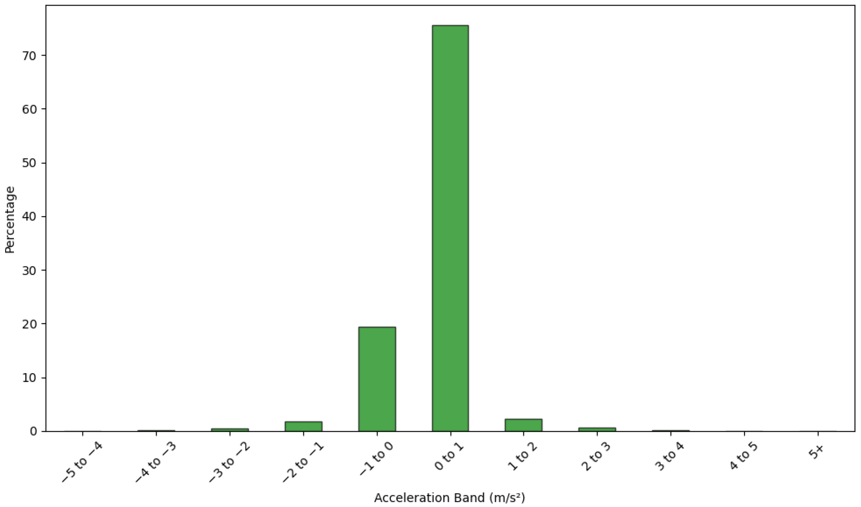
Touch rugby is an intermittent sport, characterized by repeated transitions between high- and low-intensity activities, which can be confirmed from Figure 2, Figure 3, Figure 4 and Figure 5. According to Figure 2 and Figure 4, we can see that female and male athletes run at a velocity between 1 and 0.5 m/s for approximately 70% and 65% of the match time, respectively. At certain moments, both female and male athletes run very fast at more than 4.0 m/s. Furthermore, in Figure 3 and Figure 5, we found that during approximately 80% for females and 70% for males of the match time, the accelerations of the athletes ranged between 0 and 0.1 m/s2, indicating relatively low acceleration levels. So we can conclude that athletes are in low-intensity activity states during the majority of match time.
Figure 2.
Velocity distribution for 12 female athletes during the matches.
Figure 3.
Acceleration distribution for 12 female athletes during the matches.
Figure 4.
Velocity distribution for 15 male athletes during the matches.
Figure 5.
Acceleration distribution for 15 male athletes during the matches.
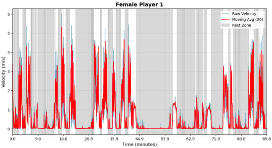
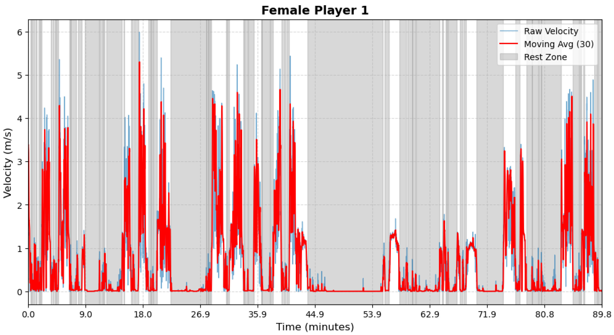
Studies show that velocity and acceleration are the key components of external workload [8,56]. In particular, high-intensity movements are the main factor that contributes to an athlete’s fatigue and increases the risk of injury [56]. Thus, given the nature of touch rugby, it is necessary to segment in-play and rest periods during matches, which can help to better understand each athlete’s performance patterns during playing and recovery periods. Dwyer and Gabbett show that walking speeds in the sport field are around 1.0 m/s for female and 1.2 m/s for male [57]. So, we define rest periods for male athletes as the interval in which their velocities are below 1.2 m/s, and a threshold of 1.0 m/s was used for female. To accurately identify dynamic patterns during both rest and in-play periods, we apply a 3 s moving average to smooth short-term fluctuations, which follows the approach used in Marutani et al.’s work [58]. After that, we apply the predefined thresholds to perform the segmentation. In addition, we apply a more rigorous definition of the in-play period, which is the time during which an athlete’s velocity exceeds the predefined threshold for more than 5 s [58].
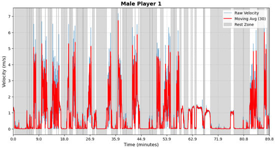
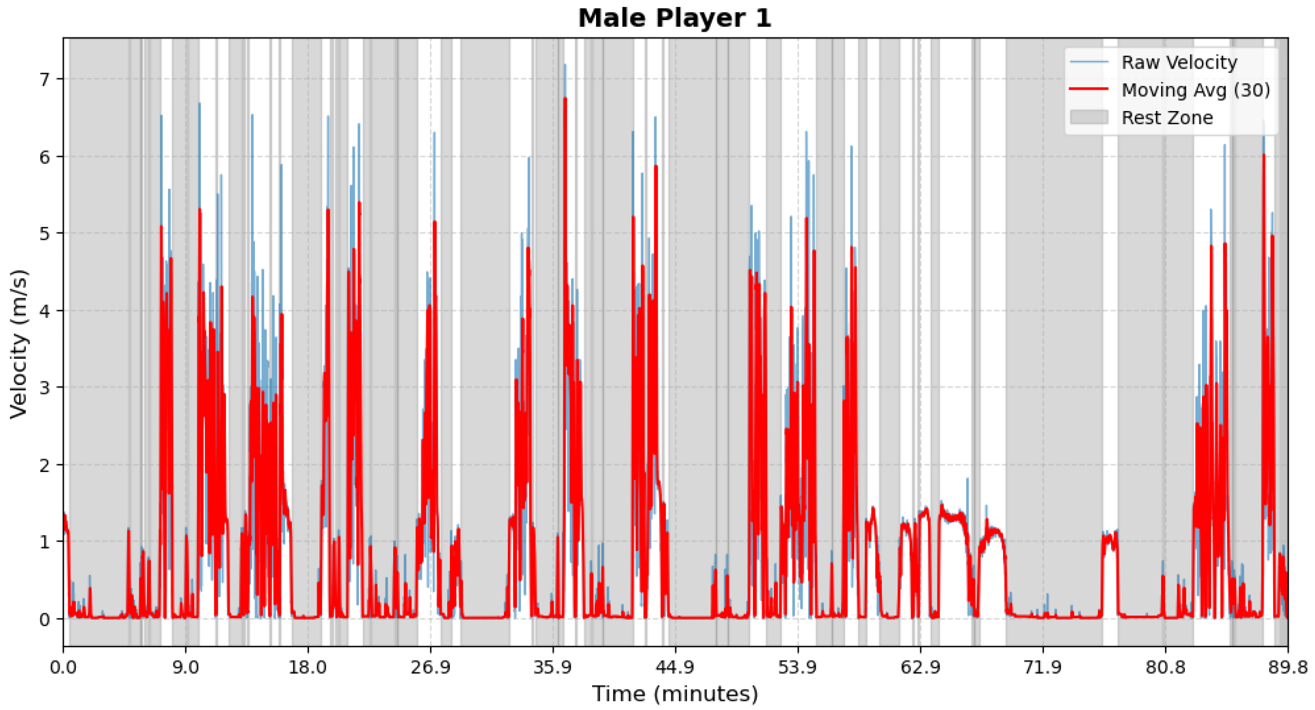
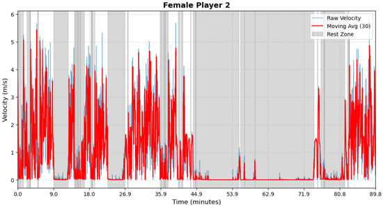
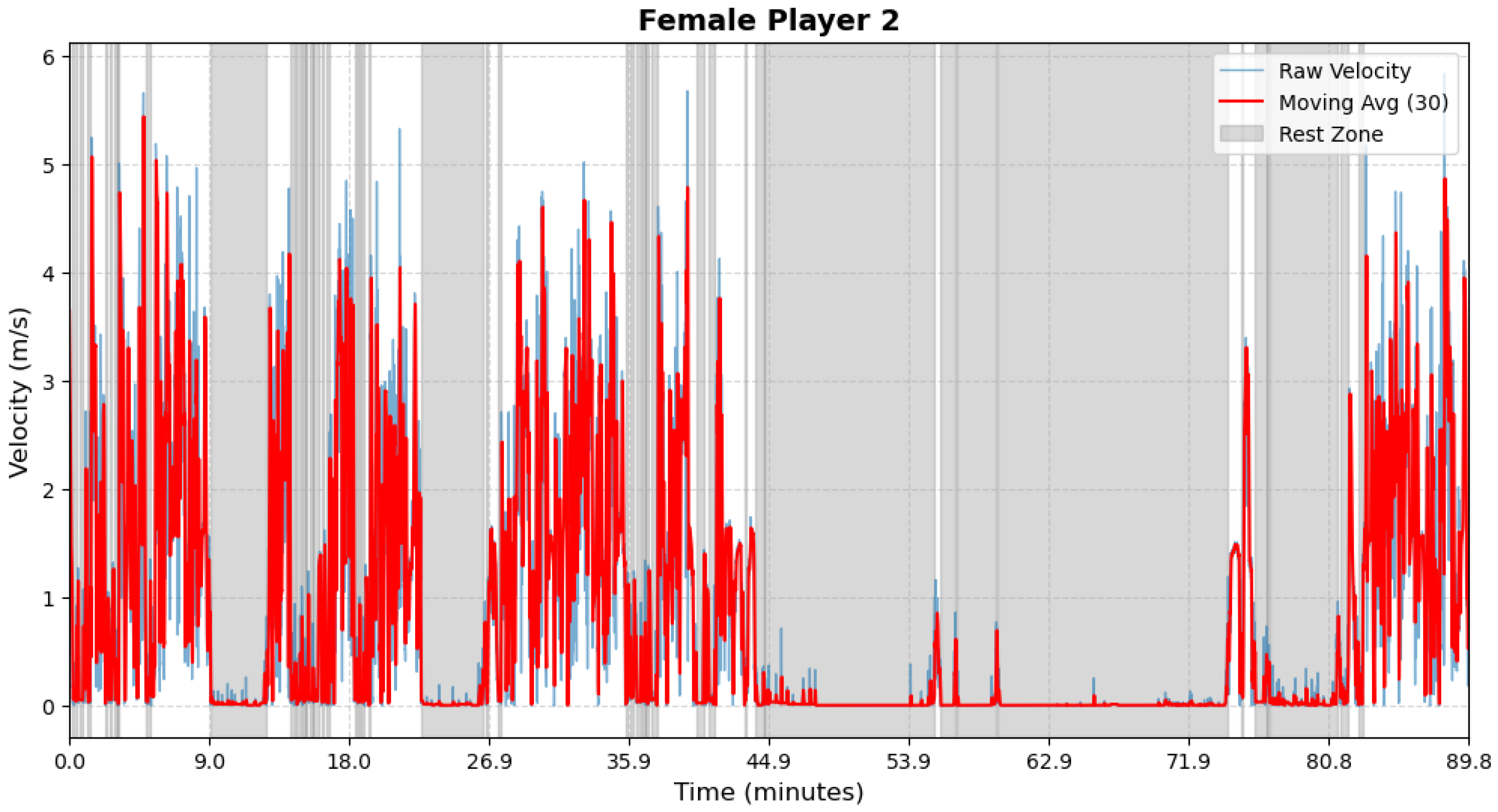
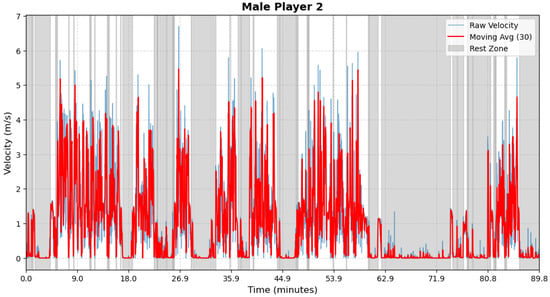
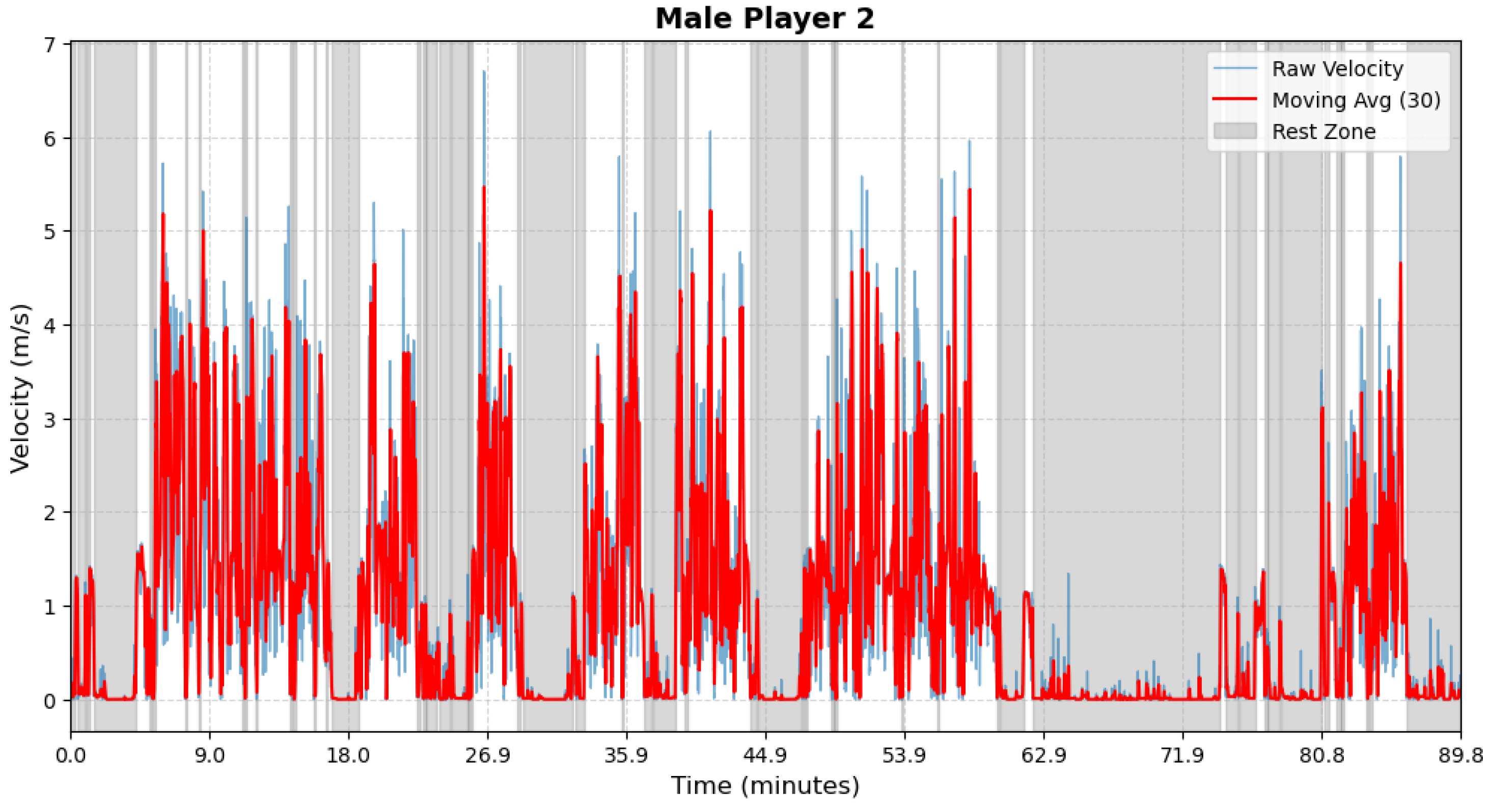
The segmentations of the entire observation period, including two matches, for one female and one male athlete are shown in Figure 6 and Figure 7. The segmentations for the remaining athletes are presented in the Appendix B. The gray and white areas in these figures represent the rest and in-play periods, respectively. The blue lines represent the 3 s moving average velocity traces. According to these figures, each athlete exhibits multiple velocity spikes intermittently throughout the entire matches. These results form the foundation for the subsequent analysis and modelling of the probability of developing fatigue (see Figure 8 and Figure 9).
Figure 6.
Female athlete 1—Period Segmentation.
Figure 7.
Male athlete 1—Period Segmentation.
Figure 8.
Female athlete 2—Period Segmentation.
Figure 9.
Male athlete 2—Period Segmentation.
4.2. Athletes’ Profiles Analysis
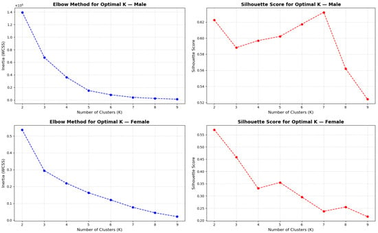
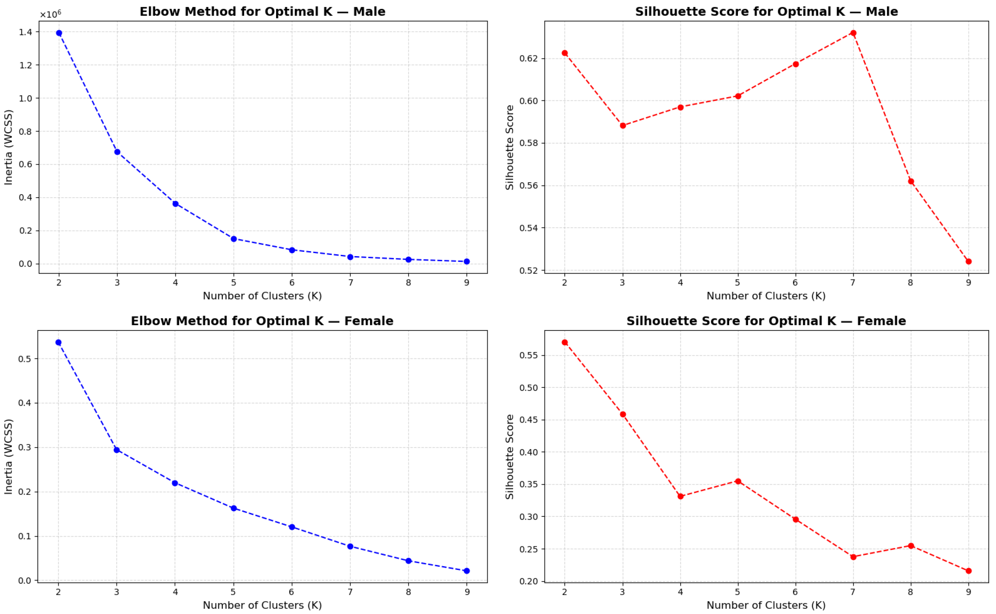
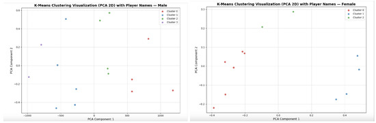
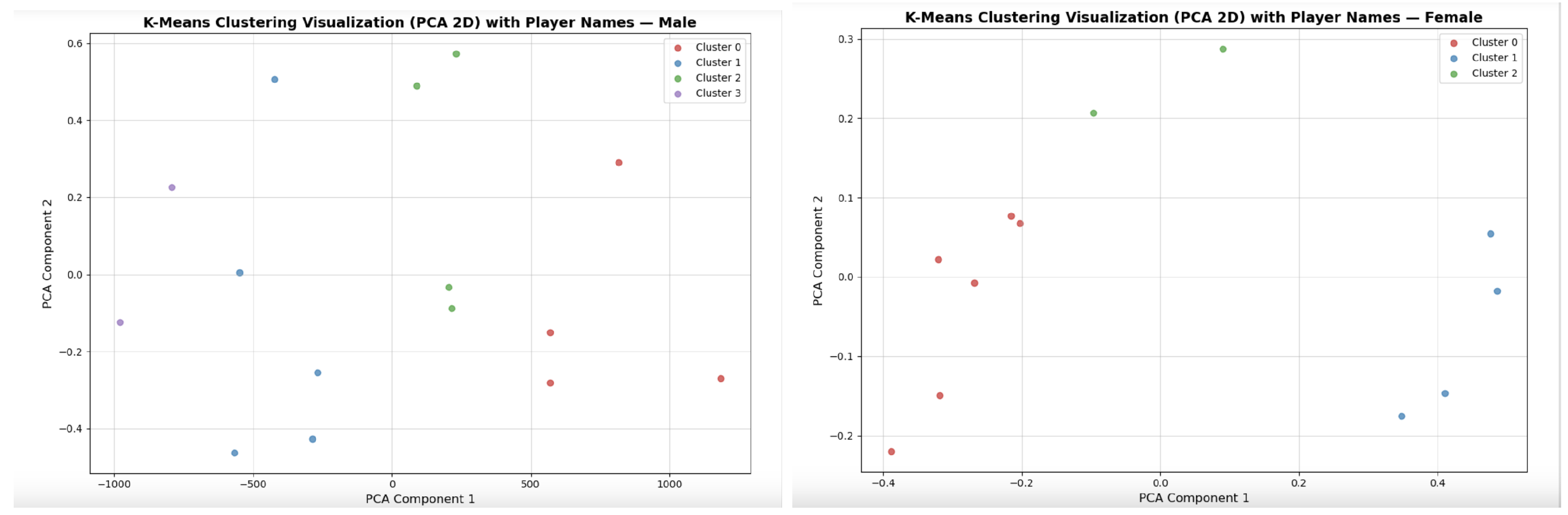
To gain a deeper understanding of the differences among athletes’ movement patterns, we apply the Gaussian Mixture Model (GMMs) to cluster velocity data taken during in-play periods into high-intensity and low-intensity phases for each athlete. The definition of in-play state refers to Section 4.1. Furthermore, in order to examine whether there is a cluster effect within the teams, we use K-means to cluster female and male athletes into 3 and 4 groups, respectively, based on the static summary information estimated from GMMs. To determine the optimal number of clusters for both male and female athletes, two methods were applied to determine the number of clusters, which are the Elbow Method and the Silhouette Score. For male athletes, the top two subfigures in Figure 10 shows that the Elbow Method indicates the largest drop in WCSS before k = 4, after which the curve was flattened. The Silhouette Score peaked at k = 7, resulting in only two athletes per group, which is too small for a meaningful analysis. Thus, K = 4 was chosen as the best trade-off between cluster quality and group size. Following the same rationale, K = 3 was selected for female athletes Based on the information presented in the bottom two subfigures in Figure 10. Furthermore, we use the Adjusted Rand Index (ARI) to consider whether the clusters are stable and reliable. We perform k-means clustering with 50 random initial values on the female and male data separately. Then, ARI is calculated between the first result of k-means clustering and each of the subsequent solutions. The mean ARI is 0.847 (>0.75) for the female group, indicating moderate, stable, and robust clustering solutions. And 0.976 (>0.9) for the male group, showing a highly stable clustering structure. Moreover, Figure 11 illustrates the resulting cluster assignments visualized in two-dimensional PCA space for male and female athletes, respectively. According to these two figures, it is evident that the clusters exhibit distinct patterns among male and female athletes. Each cluster can be clearly distinguished in terms of velocity-related metrics, reflecting distinct activity intensity patterns among the groups. More detailed information is shown in Table 1 and Table 2 below.
Figure 10.
Elbow Method and Silhouette Score for male (top) and female (bottom) athletes.
Figure 11.
K-Means clustering visualization (PCA 2D) for male (left) and female (right) athletes.
Table 1.
Summary statistics for female athletes by clusters.
Table 2.
Summary statistics for male athletes by clusters.
Table 1 illustrates three identified clusters for female athletes based on velocity data over the entire observation period, with Cluster 0 including 6 athletes, Cluster 1 including 4 athletes, and Cluster 2 including 2 athletes. From this table, we can see that each female cluster exhibits different movement patterns. First, Cluster 0 is characterized by relatively higher values in terms of , and they spend more time in the low-intensity phase than in the high-intensity phase. Second, among the clusters, Cluster 1 exhibits lower velocity standard deviation in the low-intensity phase and higher standard deviation in the high-intensity phase. Third, compared with the other clusters, Cluster 2 exhibits lower velocity variation in the high-intensity period.
The male athletes are grouped into four clusters, as shown in the Table 2, based on the whole observed velocity data. Cluster 0 comprises 4 athletes, Cluster 1 comprises 5 athletes, Cluster 2 comprises 2 athletes, and Cluster 3 comprises 4 athletes. According to this table, male athletes also exhibit different movement patterns for the different clusters. First, Cluster 0 is characterized by the highest average speed during the in-play period. Second, during the high-intensity period, Cluster 2 exhibits the lowest velocity standard deviation among the clusters. Third, Cluster 3 has lower and higher than the other clusters.
5. Results and Discussion
This section presents the model estimation results and model performance comparison, followed by a post-model analysis. The key findings are then examined and discussed in the context of the research objectives to highlight their practical implications.
5.1. Model Estimation and Evaluation
The parameters are estimated using the procedure described in Section 3 and calibrated using the dataset described in Section 4 with the halftime break excluded. All parameters in the models mentioned in Section 3.3 have been estimated, and the results are shown in Table 3.
Table 3.
Parameter estimates.
From Table 3, except for , we can see that the remaining parameters have relatively small standard deviations, indicating that the parameters have been accurately estimated. The frailty term and covariates are significantly associated with the risk of entering workload spike state, as their corresponding p value is less than 0.05. We also find that both 3 s lagged velocity variation over 30 s and 10 s lag continuous time spent in the spike state are significant predictors of the likelihood of transitioning into the next workload spike state. What’s more, the estimated results for all proposed models show that a greater 3 s lagged velocity variation over 30 s increases the probability of entering the workload spike state. For example, in the FM model, if the other conditions remain unchanged, then a unit increase in the past standard deviation of the velocity is associated with a 55.12% which equals increase for male athletes and 71.60% which equals increase for female athletes, respectively, in the hazard rate of entering the workload spike state. Regarding the parameter , we find that the value of is estimated relatively small among all models with a frailty term, suggesting that there is limited unobserved heterogeneity while still contributing to explain variation across the Cluster. Furthermore, based on the estimated results for our most complex model (TSFM model), and in the TSFM model for both male and female are estimated to be negative, indicating that an increase in 3 s lagged velocity variation over 30 s and 10 s lag continuous exposure to the spike state will speed up to the point of entering the workload spike state.
Table 4 shows the evaluation of the performance of the proposed model using AIC, BIC, deviance explained, and REML. Three key observations can be drawn from this table. First, models incorporating covariates perform better than those without covariates. This indicates that the likelihood of transitioning into the workload spike state is influenced by the covariates for both female and male athletes’ data. Second, the hazard rates exhibit a cluster-level effect, as models incorporating a cluster-specific frailty term show lower AIC and BIC values, as well as a higher deviance explained rate and REML compared to models without the frailty term, while all other settings remain the same. The discussion of frailty terms with alternative distributions, the Gamma distribution, is provided in Appendix C. Third, the TSFM model consistently outperforms all other proposed models as it achieves the lowest AIC and BIC values while also exhibiting the highest explained deviance. This implies that both covariates impact the time to enter the workload spike state and observable cluster-specific effects in the data.
Table 4.
Model comparison for male and female athletes.
To evaluate the predictive accuracy, we computed the time-dependent AUC () and the integrated AUC (iAUC) by following the method described in the study of Heagerty and Zheng [60]. The full dataset with the halftime break excluded is used in this calculation. The calculated results are shown in Table 5. From this table, we can see that the TSFM model consistently achieves higher AUC(t) values across different time points ( min), compared with other models for both female and male data. In addition, the iAUC values of the TSFM model are the highest, with 0.805 for female and 0.818 for male. Combining these two points, we conclude that the TSFM model provides a more accurate prediction of event risk compared to alternative models.
Table 5.
Time-dependent AUC at selected time points and iAUC.
5.2. Post-Model Analysis
In this section, we perform a post-model analysis on cluster-specific frailty terms, hazard baselines, and the partial effect of the factor presenting past information about continuous exposure time in the workload spike state. The following analysis is based on the data described in Section 4 with the halftime break excluded.
5.2.1. Cluster-Specific Frailty Analysis
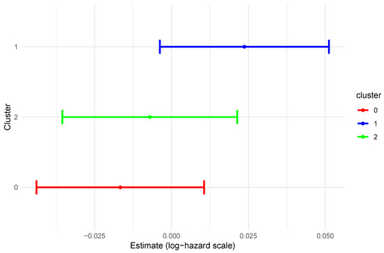
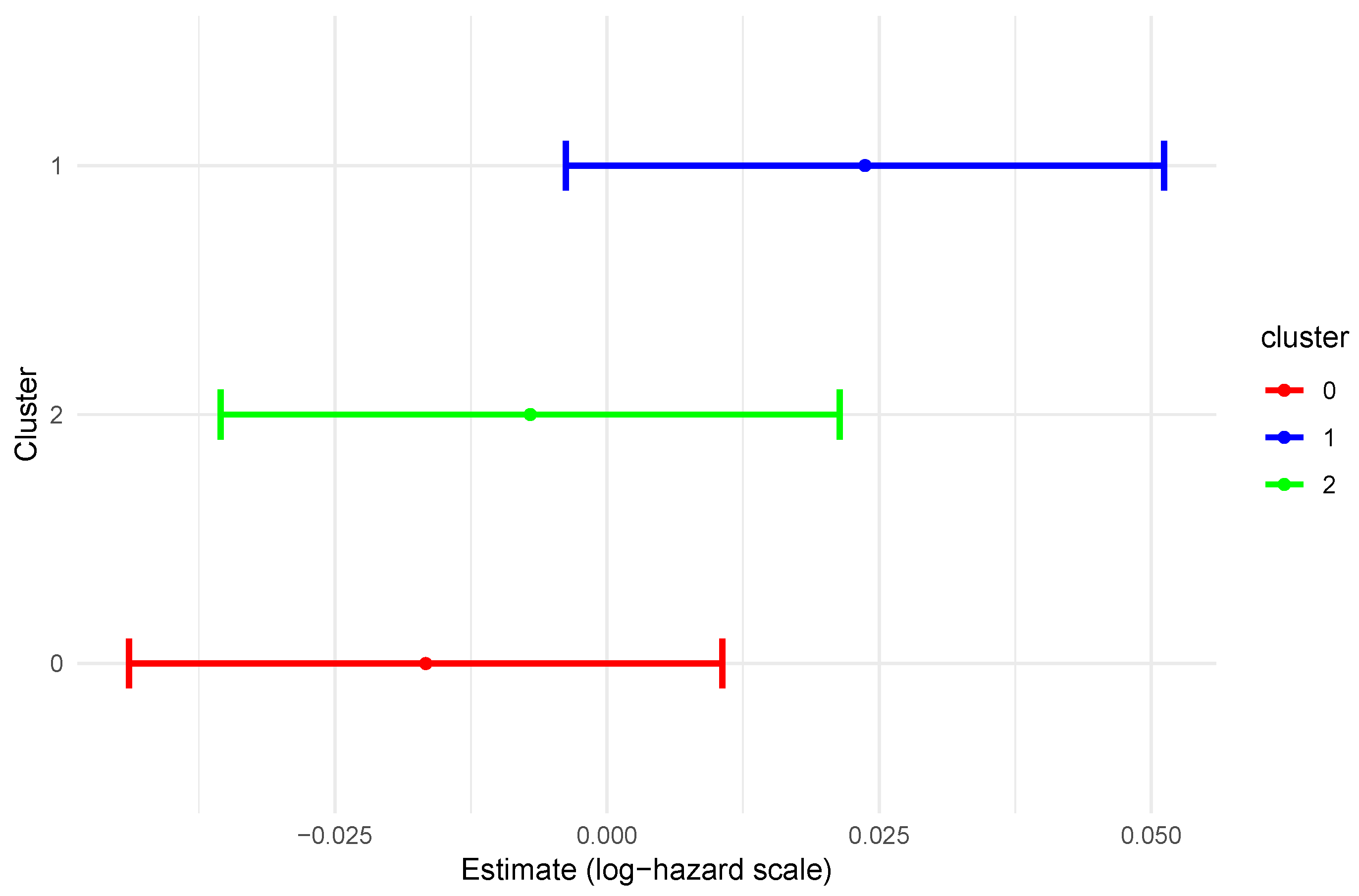
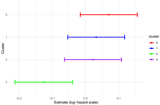
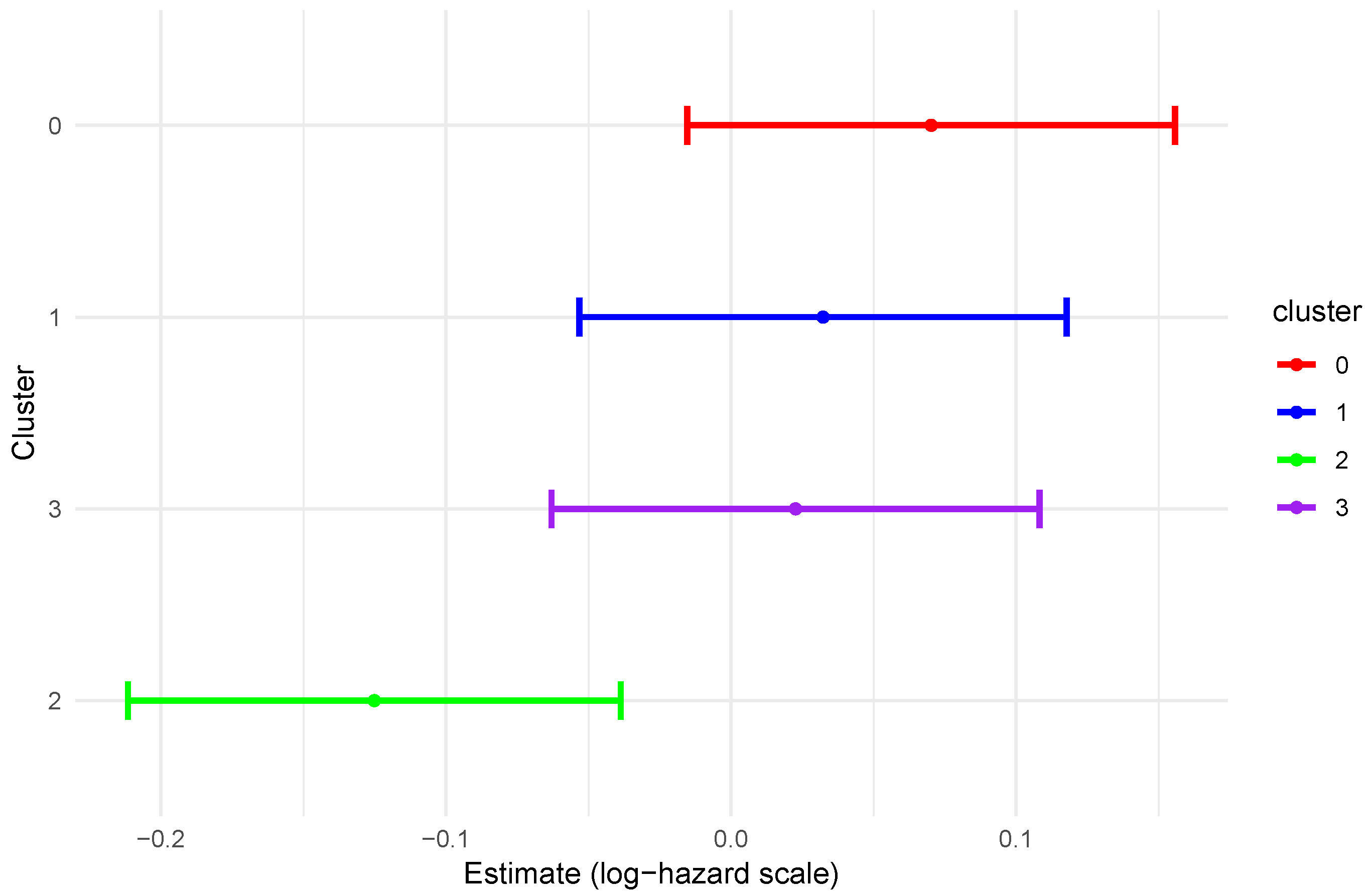
Figure 12 and Figure 13 present the cluster-specific frailty term (random effects) with 95% confidence intervals, which is used to quantify an unobserved heterogeneity between clusters. Among female athletes, Cluster 1 demonstrated a positive frailty estimate that exceeded all other clusters, suggesting a baseline risk exceeding what is predicted by covariates alone and greater than that of other clusters. Furthermore, the frailty terms for Clusters 0 and 2 are estimated to be negative, suggesting that they have lower baseline hazards than the average risk.
Figure 12.
Random effects (frailty) estimates for female clusters with 95% confidence intervals.
Figure 13.
Random effects (frailty) estimates for male clusters with 95% confidence intervals.
In male athletes, positive frailty was estimated for Clusters 0, 1, and 3, indicating that the baseline hazards of these three clusters are higher than average risk, with Clusters 1 and 3 showing similar estimated frailty values. The similar frailty estimates suggest low heterogeneity in baseline hazard between these two clusters. In addition, Cluster 0 shows the largest positive frailty effect such it has a higher baseline risk compared to all other clusters. In contrast, the estimated frailty term of Cluster 2 is negative and the lowest among all clusters, so this cluster has the lowest baseline risk of transitioning into the workload spike state. This is possibly because Cluster 2 is clearly distinct, exhibiting lower variability during high-intensity periods and a more stable workload pattern, which likely contributes to its lower frailty values. This may also be due to unobserved factors, such as individual physiological characteristics or recovery practices, which were not captured in the dataset.
5.2.2. Baseline Hazard Analysis
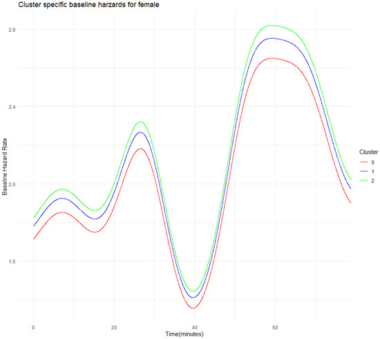
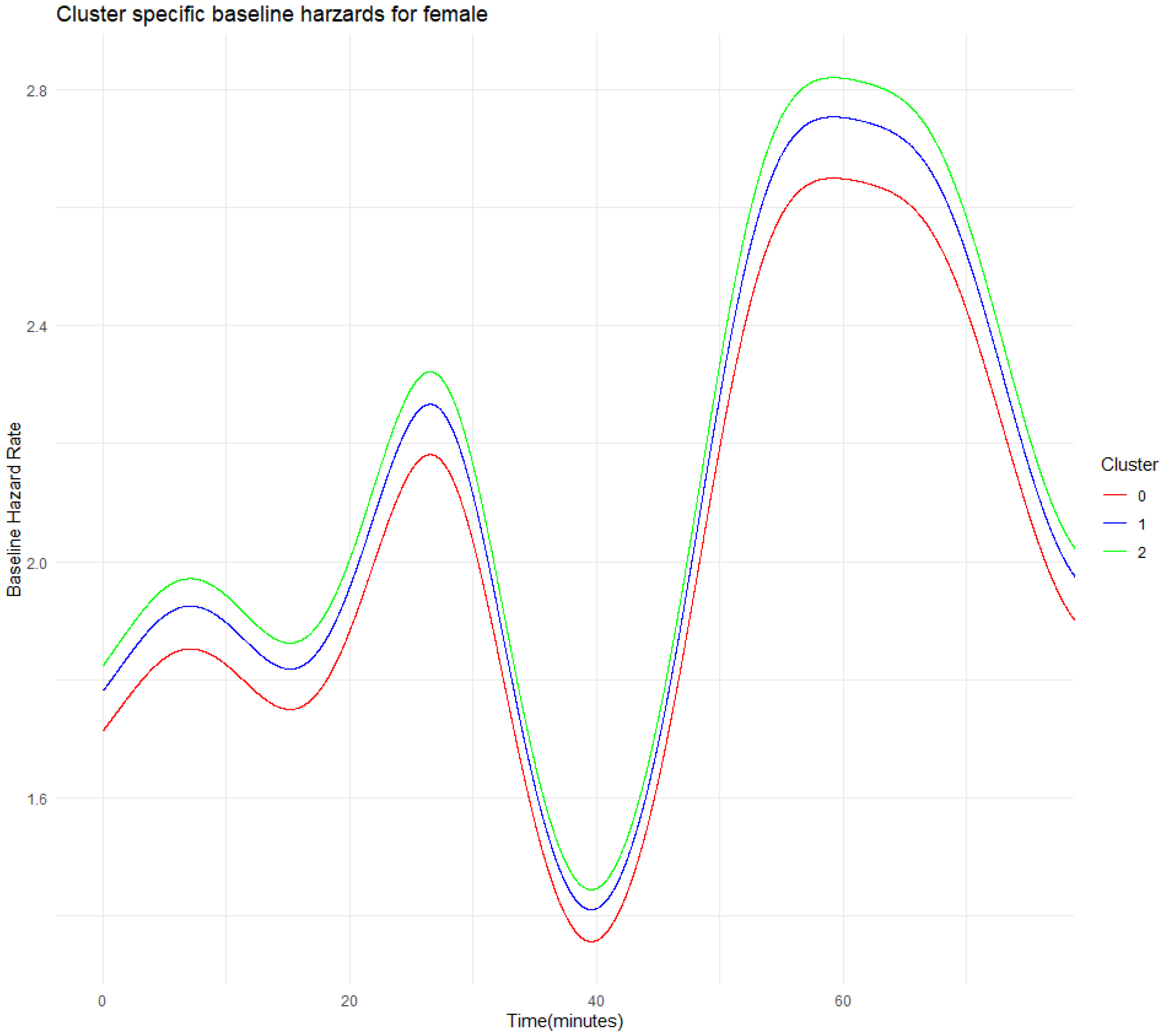
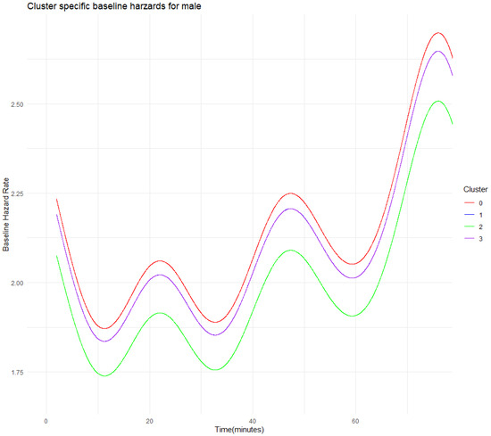
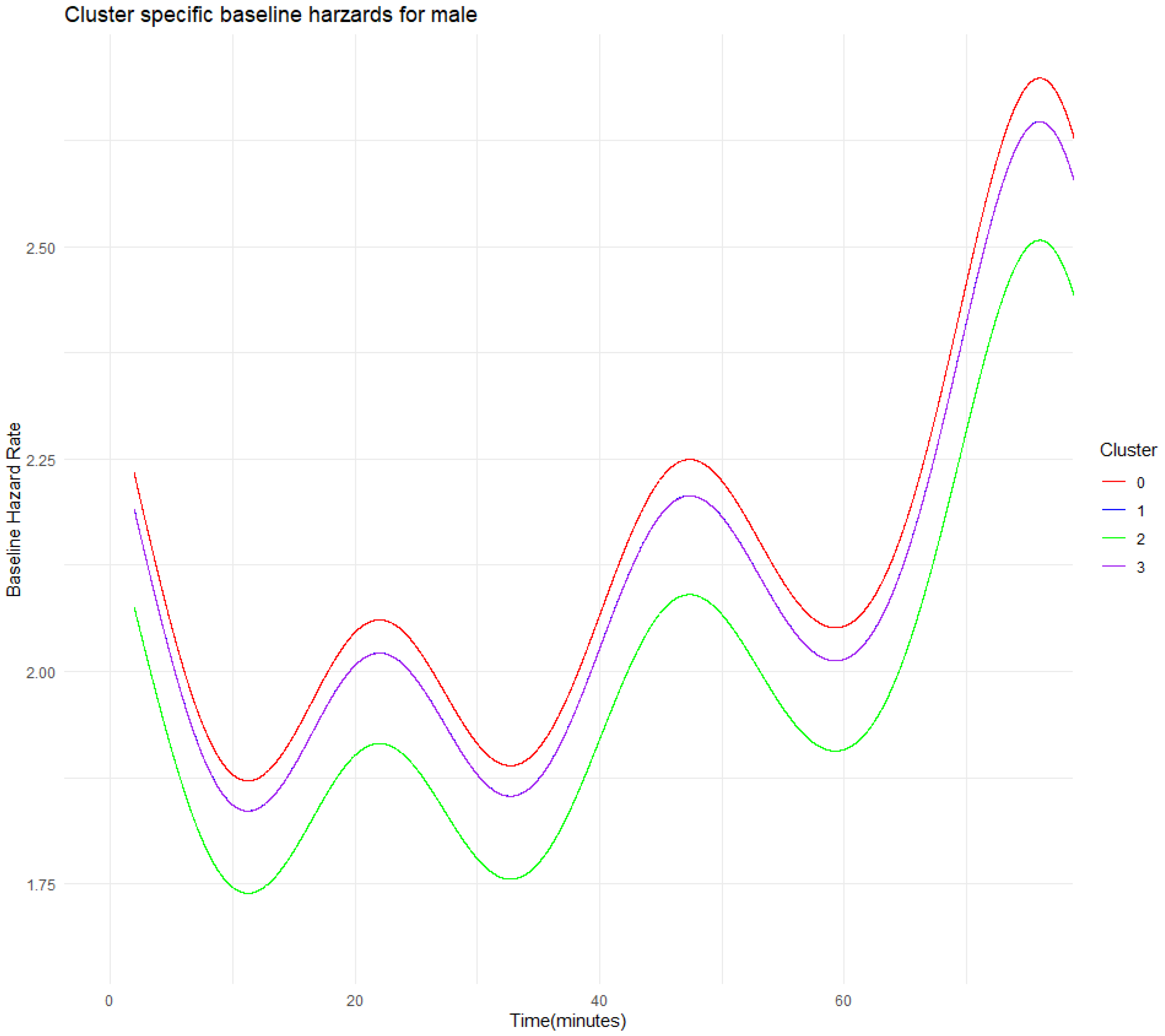
The baseline hazard rate reflects the instantaneous injury risk regardless of the individual athlete’s movement behaviour, which is the foundation of our proposed models. The estimated baseline hazard rates are illustrated in Figure 14 and Figure 15 and stratified by cluster for female and male athletes, respectively. The baseline hazard rates shown in these two figures are aggregated data from two matches. The baseline hazard differs across clusters only by a multiplicative scaling factor, implying that they share the same underlying temporal shape, which is aligned with our model assumption. We also observe that the baseline hazard rates change over time across all clusters, suggesting that the risks of entering the workload-spike state are dynamic. We also observe that, in general, the risk during the first match (first 40 min) is lower than in the subsequent match within the same match season for both female and male. This indicates that participating in a greater number of matches within the same season leads to the accumulation of fatigue, thereby increasing the associated risk. Note that the baseline hazard curves for Clusters 1 and 3 in Figure 15 are very close but not identical, with the blue line being slightly higher. This is because the estimated frailty values for Clusters 1 and 3 differ only slightly, as discussed in the previous section.
Figure 14.
Cluster-specific baseline hazard estimates for female athletes.
Figure 15.
Cluster-specific baseline hazard estimates for male athletes.
5.2.3. Partial Effect Analysis
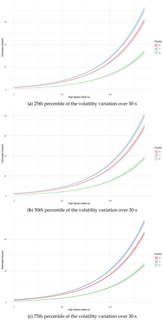
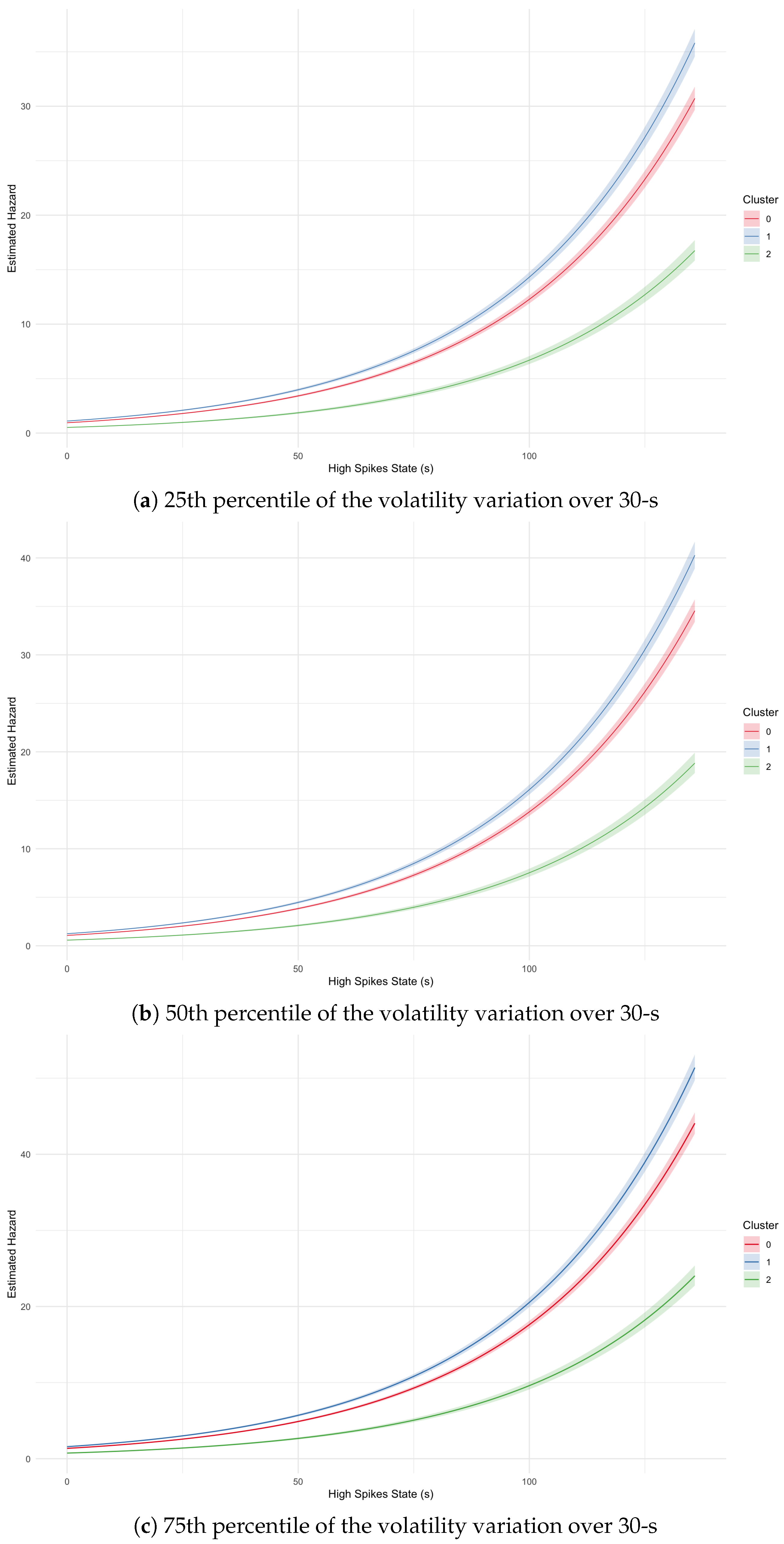
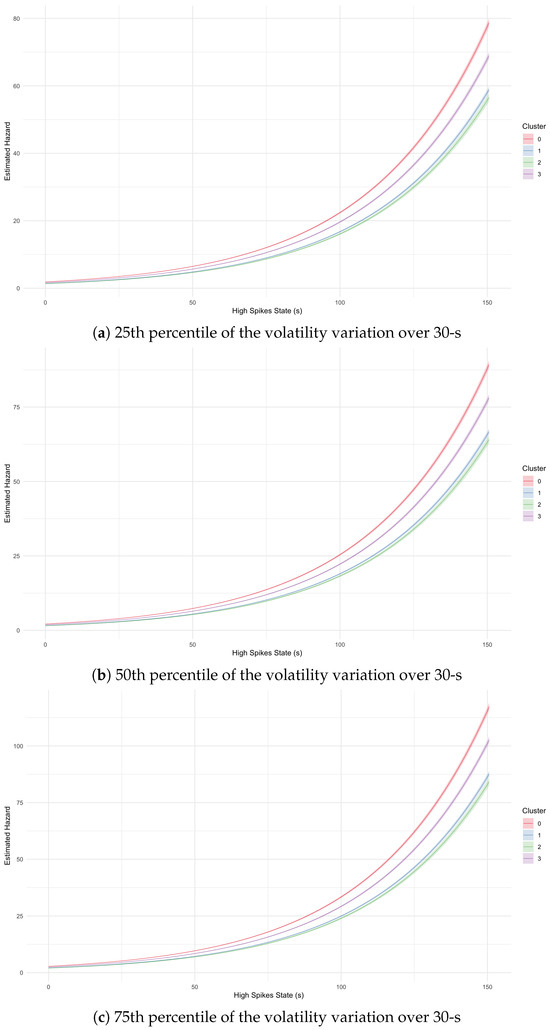
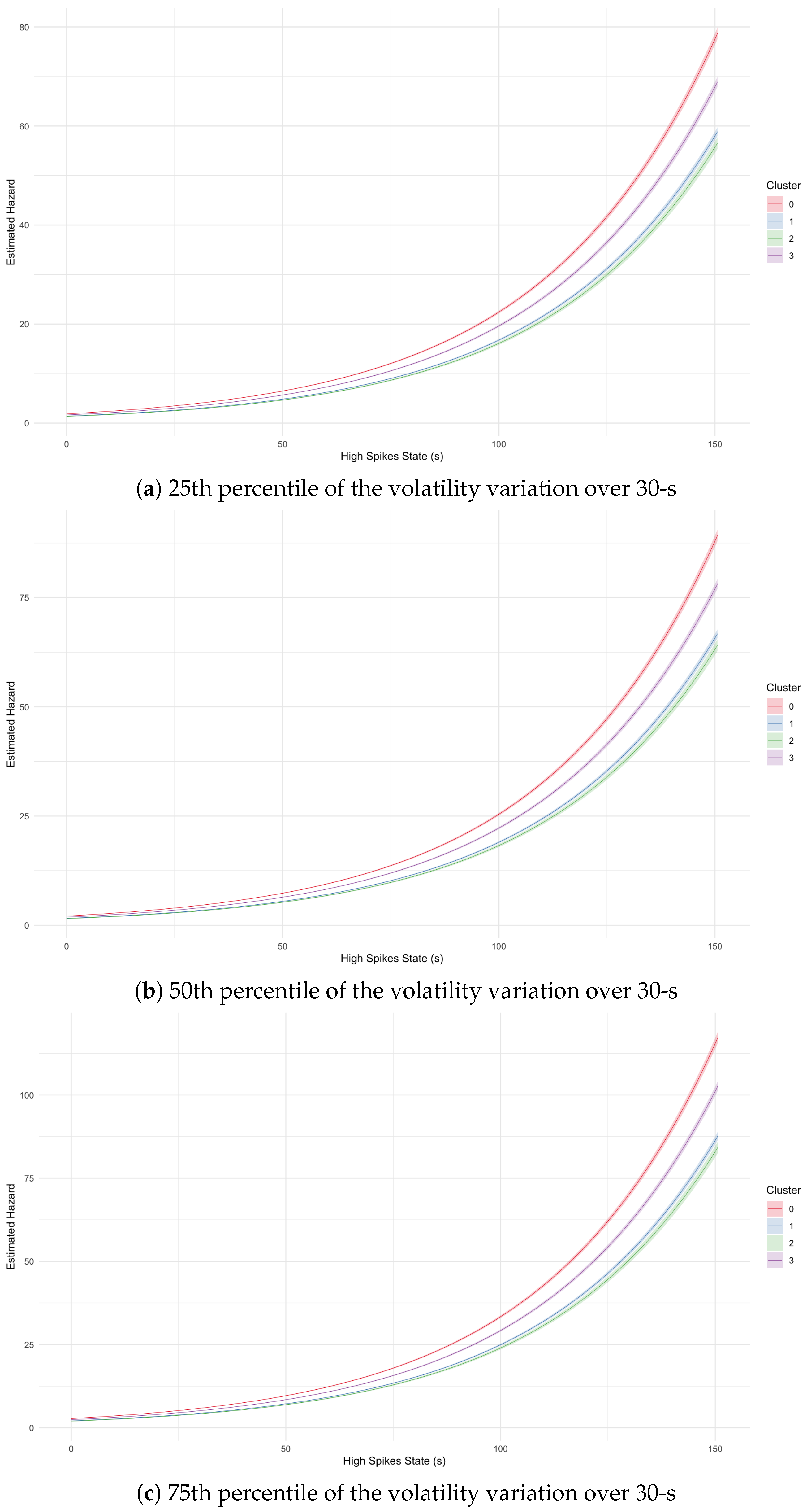
Based on the analysis of the baseline hazard rates, we now investigate the partial effect of the time of continuous exposure to the spike state to understand how this factor independently impacts the risks. We specifically focus on the partial effect of this factor, as evidenced by the results presented in Section 5.1. According to Table 4, we find that incorporating this factor into the model leads to a greater improvement in model performance compared to the other factor. To isolate this effect, we fix velocity variation at three different levels—the 25th, 50th, and 75th percentiles from the historical velocity variation data—and evaluate the TSFM model across a range of cumulative high-workload durations from 0 to 150 s using the estimated parameters from Table 3. The calculation results are presented in Figure 16 and Figure 17. The hazard rates in Figure 16 and Figure 17 exhibit a non-linear and monotonically increasing relationship with longer continuous exposure to the spike state across all clusters. The hazard rates in Figure 16 and Figure 17 exhibit non-linear, accelerating relationships with cumulative duration across all clusters. Furthermore; comparison of panels (a–c) within both figures suggests that the hazard rate rises more quickly as the velocity variation level increases, for both male and female athletes. Furthermore, the shaded bands around each plotted curve represent 95% confidence intervals for the estimated hazard. The intervals are narrower at lower values of continuous time in spike state with 10 s lag, indicating that the estimates are more reliable. However, as increasing in the value of continuous time in spike state with 10 s lag, the intervals get wider for both female and male clusters, showing considerable variability in the estimates. This may be due to the limited number of observations at longer continuous times in the spike state with a 10 s lag; additional data are needed to further validate the model. Moreover, the curves corresponding to different clusters remain distinct, with no crossing. This suggests that the differences between clusters are statistically significant.
Figure 16.
Partial effects of cumulative high-workload duration on hazard for female athletes across different velocity variation levels.
Figure 17.
Partial effects of cumulative high-workload duration on hazard for male athletes across different velocity variation levels.
6. Conclusions
Survival models have been widely applied in the field of sports analytics to predict injury. In this study, we extend the traditional survival model to a more general workload-injury framework, which incorporates the transition between 3 states: non-injury, workload spike, and injury states. We allow for mutual transit between the non-injury and workload spike states. However, we do not allow for the transition from the injury state to the other two states. These designs are motivated by our empirical observations and the characteristics of the movement pattern in touch rugby matches. That is, athletes frequently transit between high- and low-intensity activities during matches.
We then applied this framework to kinematic time-series data collected from New Zealand touch rugby matches. Due to the lack of injury information in this dataset, we use the time-scaled frailty model (TSFM) in a one-dimensional setting. The TSFM model incorporates three key components, including a time-scaling mechanism to reflect how covariates (e.g., velocity variation) accelerate or decelerate time to overload or injury; a normally distributed frailty term to capture cluster effects and unobserved heterogeneity (with potential extensions to correlated or alternative frailty distributions such as gamma); and time-varying covariates to model dynamic changes in risk factors.
Based on our model calibration and analysis results, we find that the TSFM model performs better than the other models proposed in this study. Thus, we can conclude that the 3 s lagged velocity variation over 30 s and 10 s lag continuous time spent in the spike state influences the time to the workload spike state. In addition, both time-varying covariates are found to be significant predictors of the risk of entering the next workload spike state. Furthermore, the data show evidence of a significant unobserved cluster effect across clusters for both the female and male groups.
From a practical perspective, there are three key pieces of information. First, monitoring time-lagged short-term velocity variation can help identify early signals of overload. Second, monitoring the duration of the spike state may help prevent fatigue build-up and subsequent injury risk. Third, adjusting training and substitution strategies based on shared characteristics may improve recovery planning and reduce the risk of overloading. This study provides a robust framework for identifying factors that contribute to the predefined risk and characterising underlying dynamics.
However, this study also has certain limitations, as there is no universally accepted standard definition of an overloading or workload spike event. First, in this study, an ACWR greater than 1.5 is used as the threshold to define a workload spike. It may also be defined using an alternative approach depending on the research purpose. Second, the dataset contains limited information, which constrains the scope of our analysis. A more comprehensive dataset—including longer observation periods, athlete positions, and additional factors—would enable a more detailed examination of injury risk and workload patterns. Third, although adjustments were made to account for the small sample size, further validation with larger datasets is still required. Small clusters can demonstrate information about how shared environments or consistent patterns among subjects. However, the relatively small number of subjects within each cluster may affect the stability of the estimated cluster-specific effects, limit the generalizability of the clustering results, and make it challenging to fully assess the convergence of these estimates. In addition, small sample sizes affect parameter estimates, leading to greater variability in the estimates, as reflected by wider confidence intervals. Therefore, future studies with larger sample sizes and more clusters would help validate these findings and improve the robustness of the results.
Author Contributions
Conceptualization, S.S. and T.H.; methodology, S.S.; software, T.H. and S.S.; resources, K.S.; data curation, K.S. and T.H.; writing—original draft preparation, T.H. and S.S.; writing—review and editing, N.W., S.S. and K.S.; visualization, T.H. and S.S.; supervision, S.S. and N.W. All authors have read and agreed to the published version of the manuscript.
Funding
This research received no external funding.
Data Availability Statement
The raw data supporting the conclusions of this article will be made available by the authors on request.
Acknowledgments
GenAI and Grammarly have been used for grammar checking.
Conflicts of Interest
The authors declare no conflicts of interest.
Abbreviations
The following abbreviations are used in this manuscript:
| ACWR | Acute:Chronic Workload Ratio |
| AG | Andersen-Gill Model |
| AIC | Akaike Information Criterion |
| ANOVA | Analysis of Variance |
| ARI | Adjusted Rand Index |
| BAGM | Baseline Andersen-Gill Model |
| BIC | Bayesian Information Criterion |
| BFM | Baseline Frailty Model |
| COM | Center of Mass |
| Cox PH | Cox Proportional Hazards Model |
| ES | Equivalent Slope |
| FM | Frailty Model |
| GMM | Gaussian Mixture Model |
| GPS | Global Positioning System |
| Hz | Hertz |
| iAUC | integrated AUC |
| K-means | K-means clustering |
| L-BFGS-B | Limited-memory Broyden–Fletcher–Goldfarb–Shanno with Boundaries |
| MP | Metabolic Power |
| PAMM | Piecewise Exponential Additive Mixed Model |
| PWP | Prentice–Williams–Peterson Model |
| REML | Restricted Maximum Likelihood |
| RPE | Rating of Perceived Exertion |
| SDV | Velocity variation (standard deviation of velocity) Model |
| sRPE | Session Rating of Perceived Exertion |
| time-dependent AUC | |
| TSFM | Time-Scaled Frailty Model |
| WLW | Wei-Lin-Weissfeld Model |
Appendix A. Metabolic Power Calculation
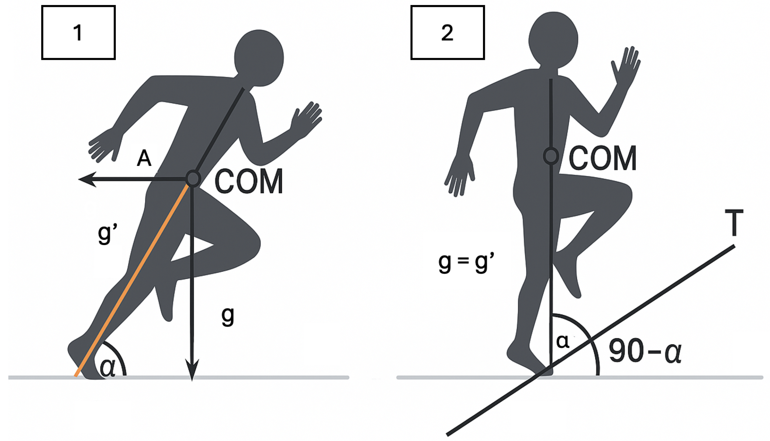
The metabolic power model under the framework of di Prampero et al. treats forward acceleration in flat terrain as energetically equivalent to constant-speed uphill running, thus capturing both speed and acceleration-related demands [8]. Figure A1 illustrates the energetic equivalence. Panel (1) shows acceleration on flat ground, and Panel (2) represents uphill locomotion with an equivalent energy cost. The slope angle , derived from the ratio , underpins subsequent energy cost computations.
The equivalent slope (ES) is given by [8]:
where is forward acceleration and g is gravitational acceleration.
Figure A1.
Energetic equivalence between forward acceleration (1) and constant-speed uphill running (2) [8]. In this Figure, COM refers to Center of Mass.
The equivalent mass (EM), which adjusts for increased muscular effort during acceleration, is computed as [8]:
The energy cost per meter (J·kg −1·m −1) is [8]:
Finally, the metabolic power (W·kg −1) is calculated as follows:
where v is the athlete’s instantaneous ground speed. This model allows for high-resolution tracking of external load.
Appendix B. Segmentation of Rest vs. In-Play Periods
The segmentation of the period for the remaining athletes in Section 4.1 is listed below.
Figure A2.
Female athlete 3—Period Segmentation.
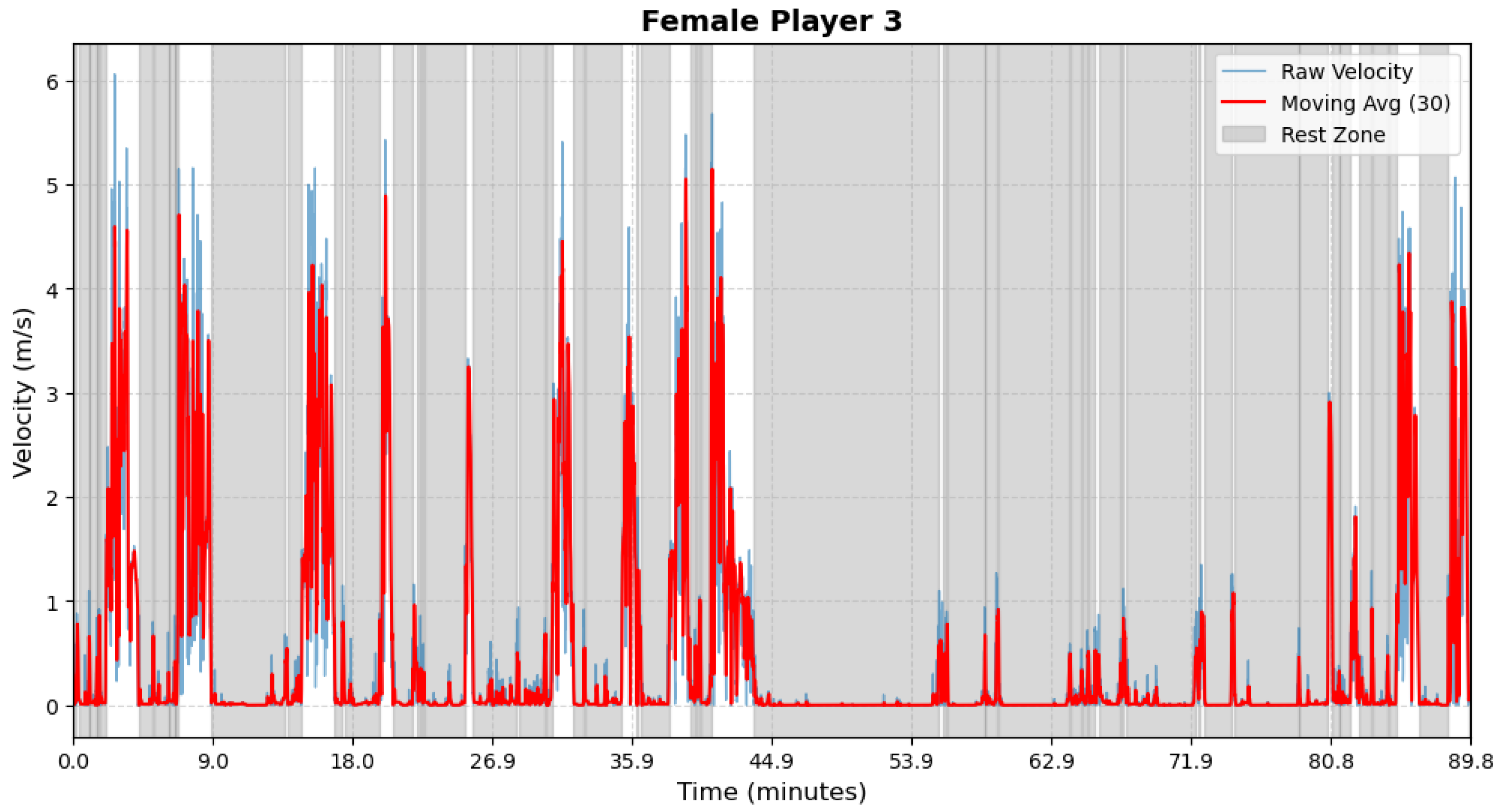
Figure A3.
Female athlete 4—Period Segmentation.
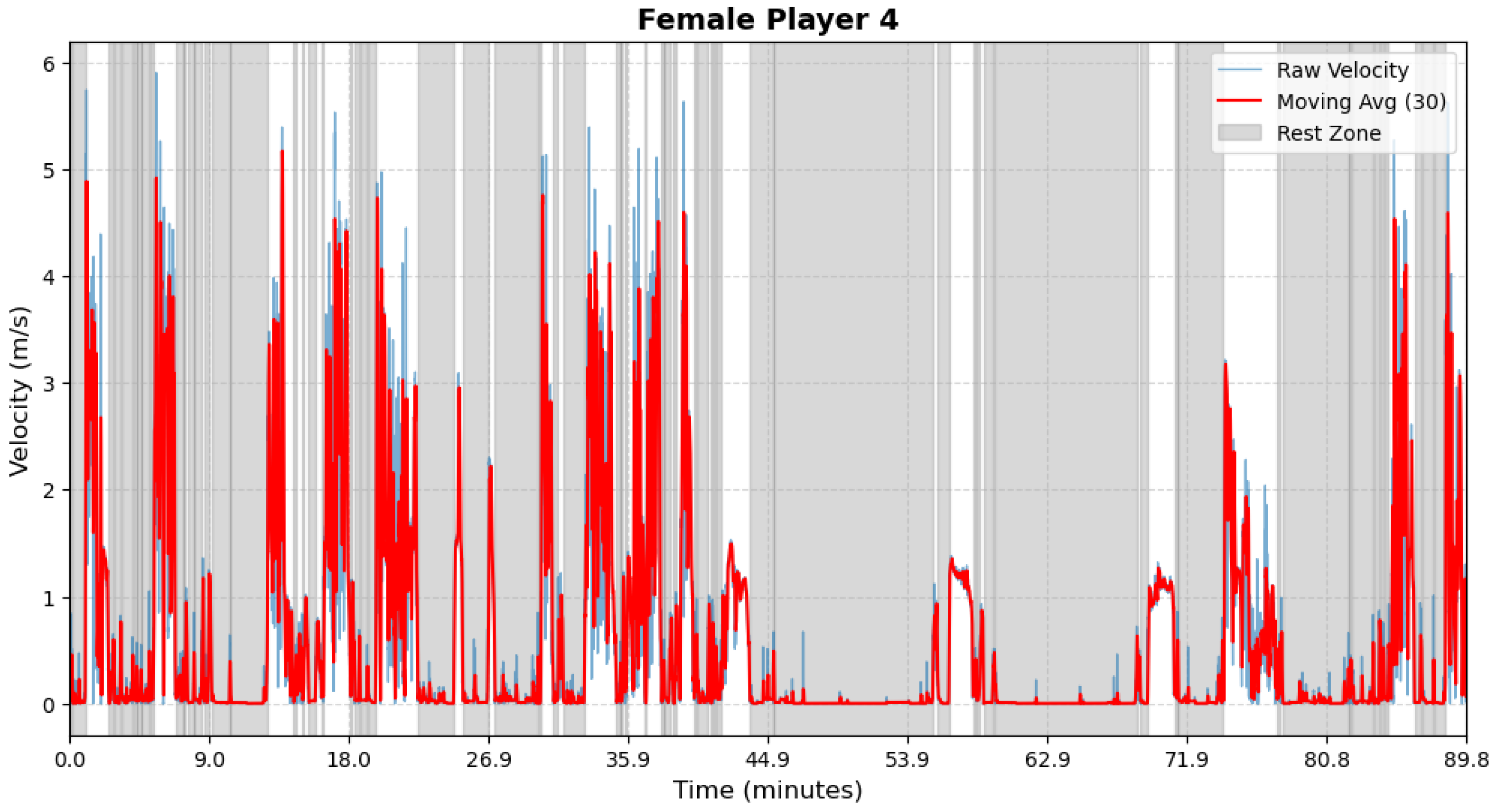
Figure A4.
Female athlete 5—Period Segmentation.
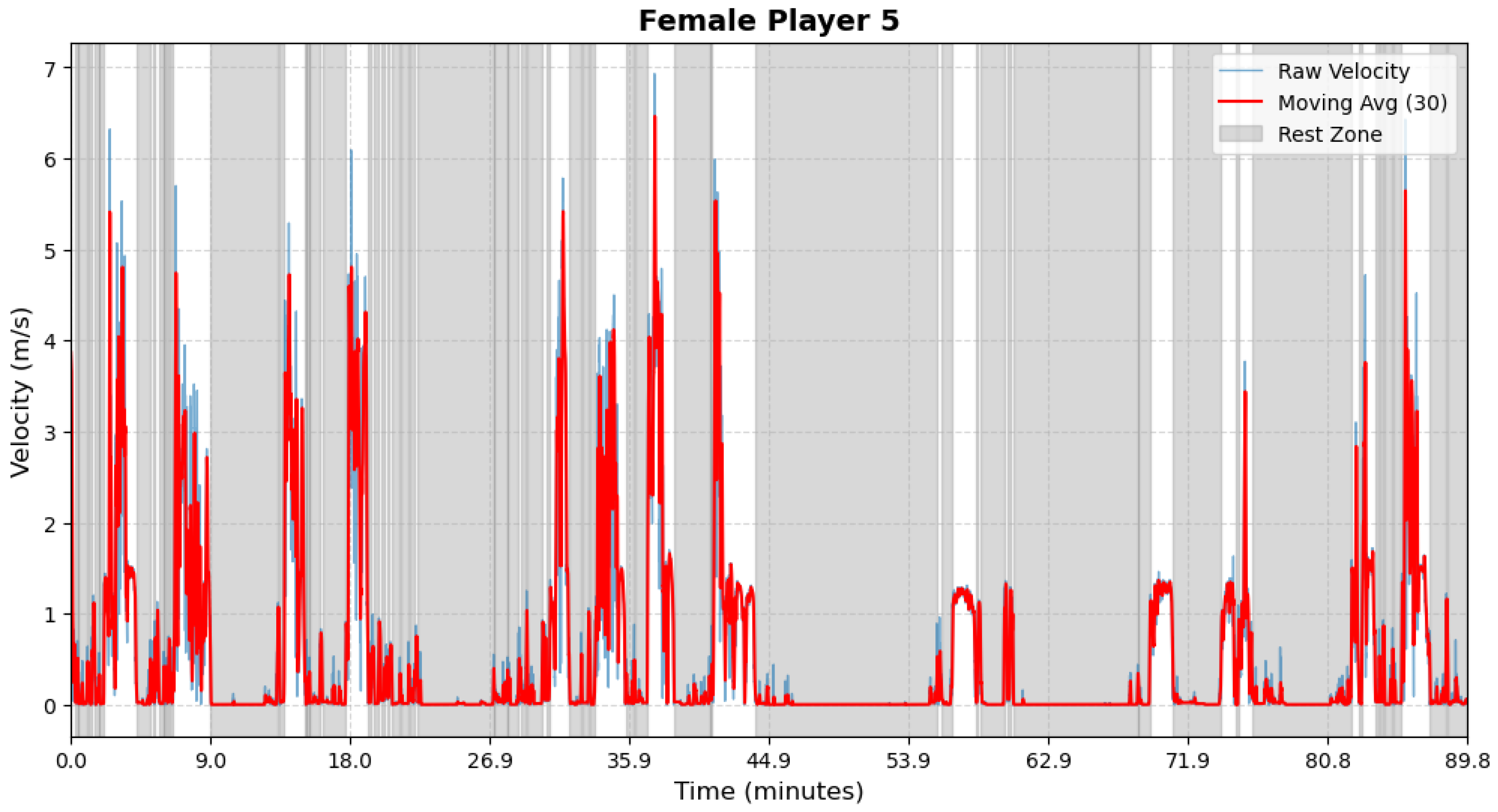
Figure A5.
Female athlete 6—Period Segmentation.
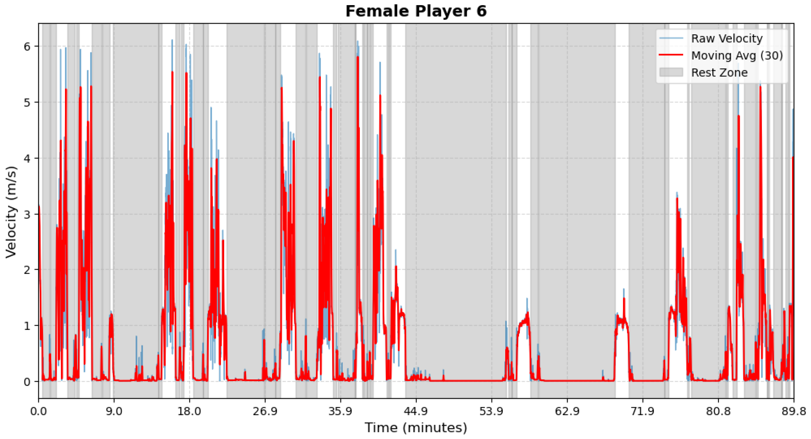
Figure A6.
Female athlete 7—Period Segmentation.
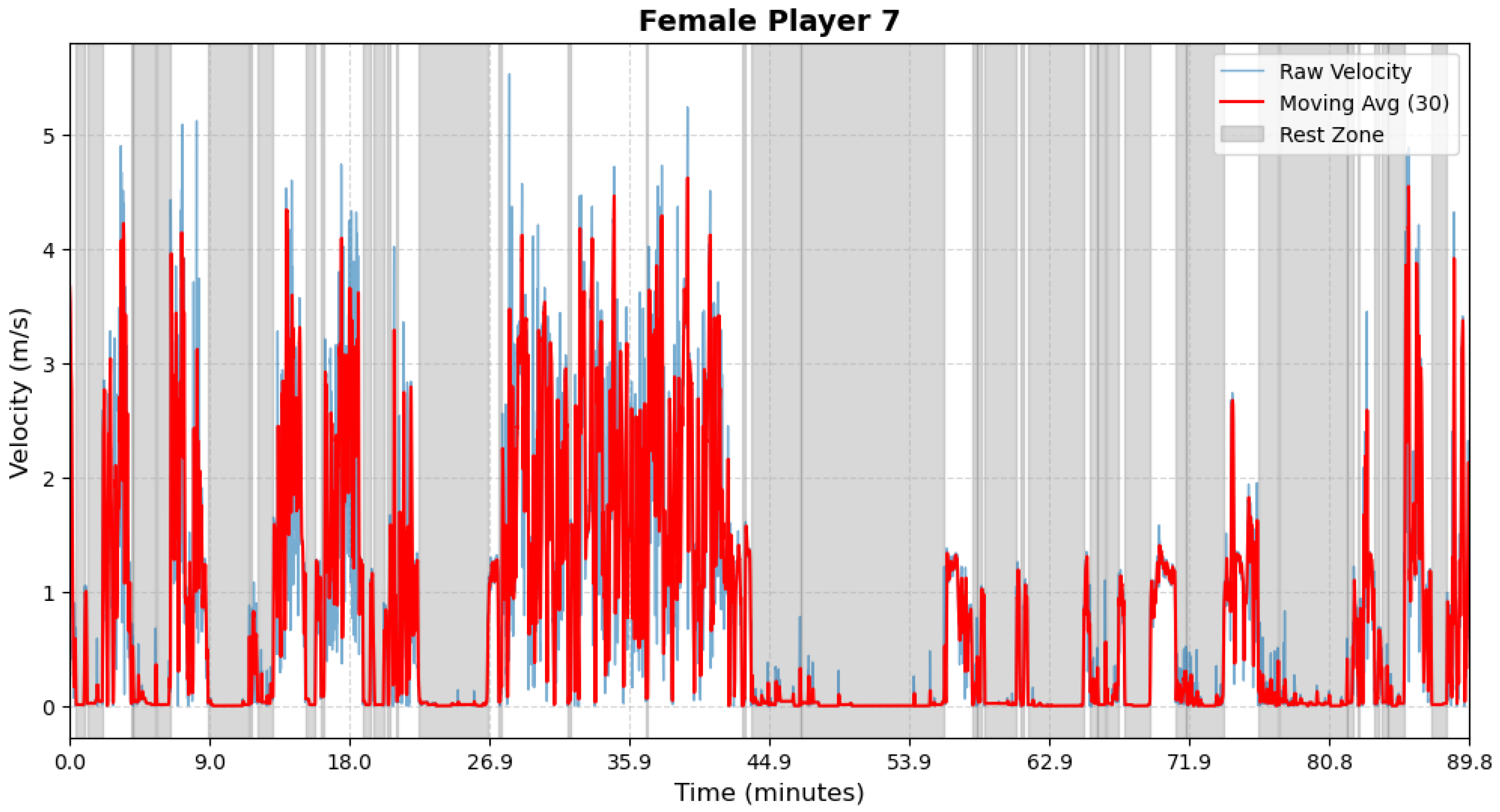
Figure A7.
Female athlete 8—Period Segmentation.
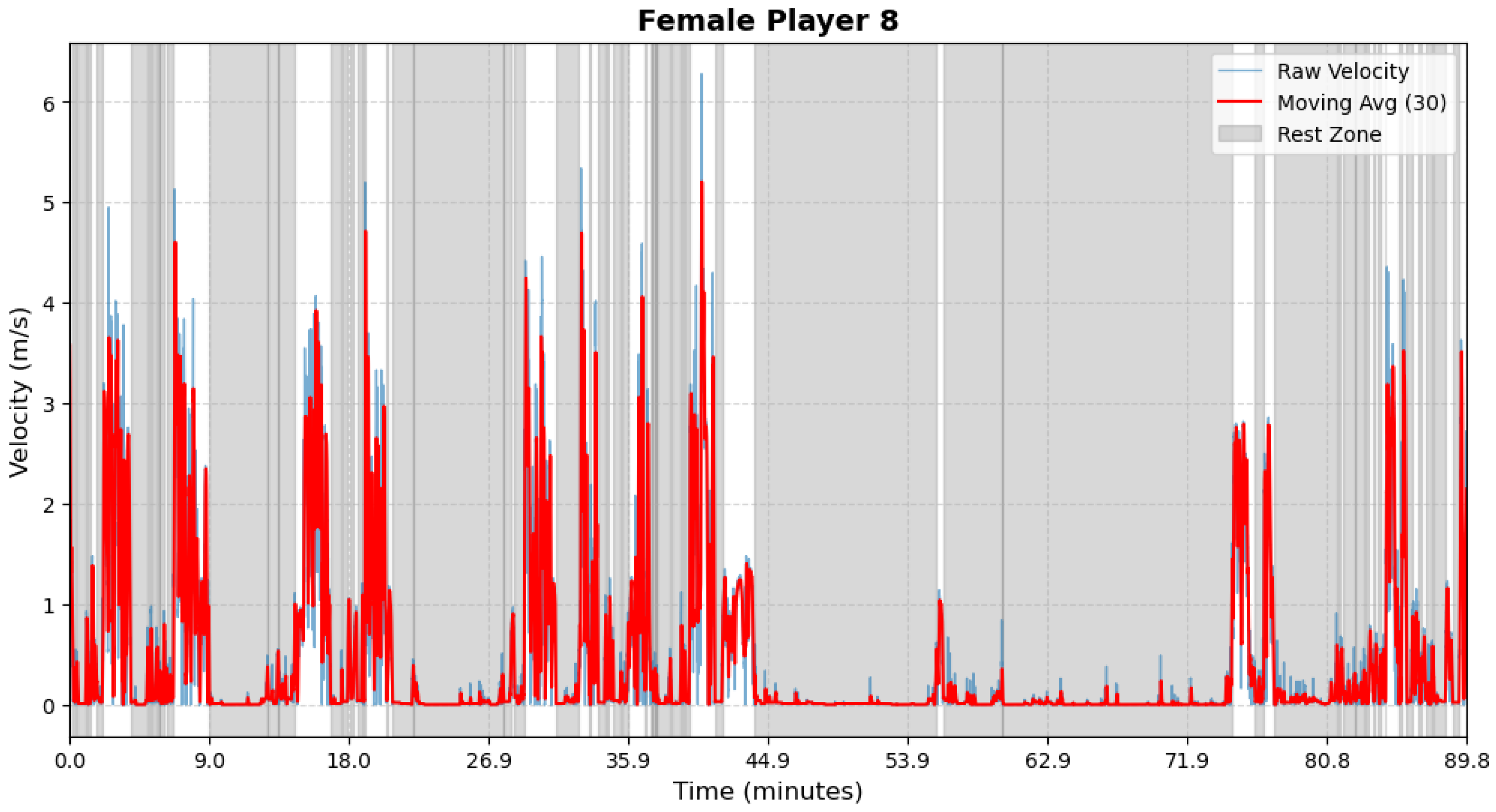
Figure A8.
Female athlete 9—Period Segmentation.
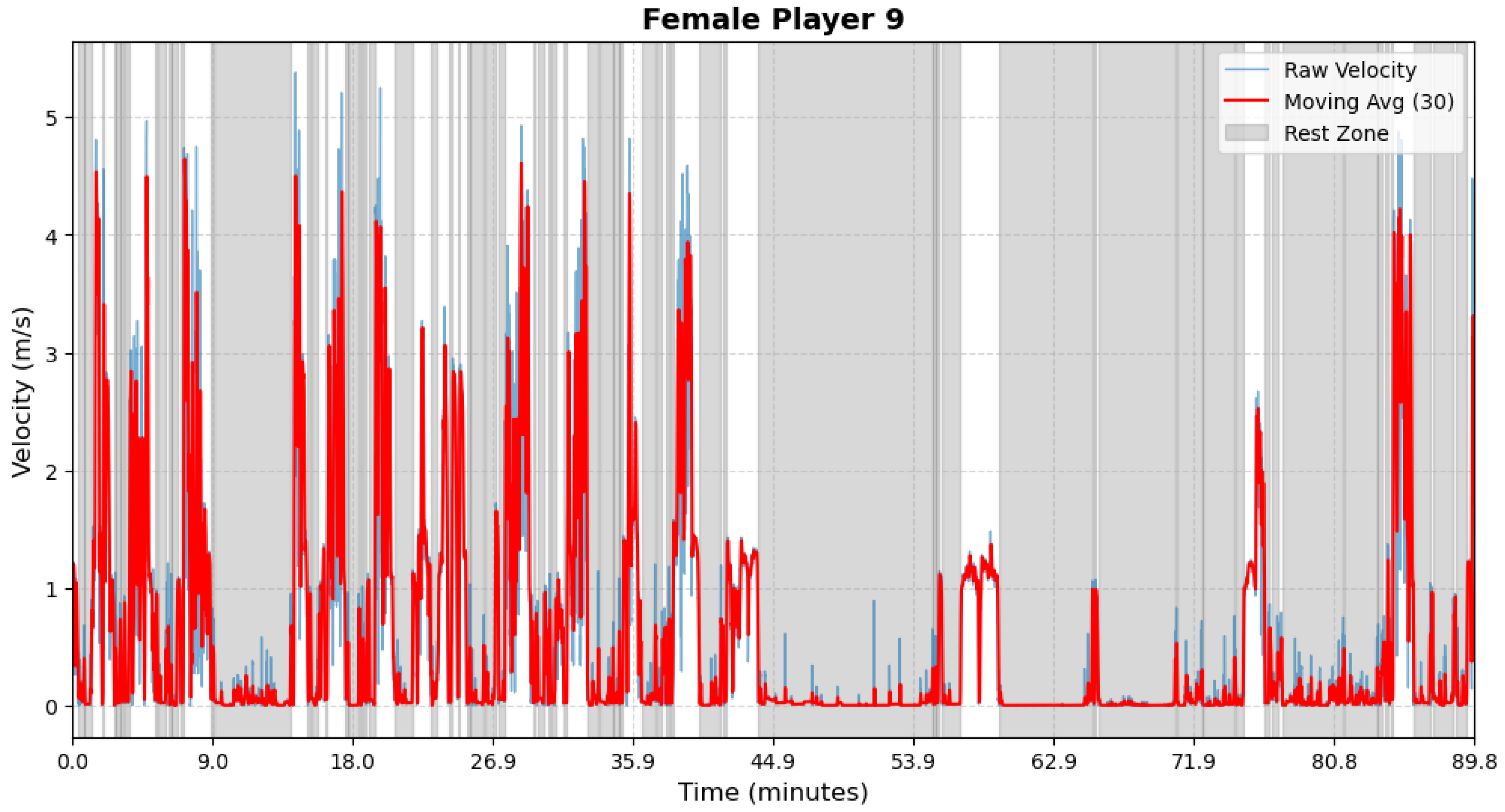
Figure A9.
Female athlete 10—Period Segmentation.
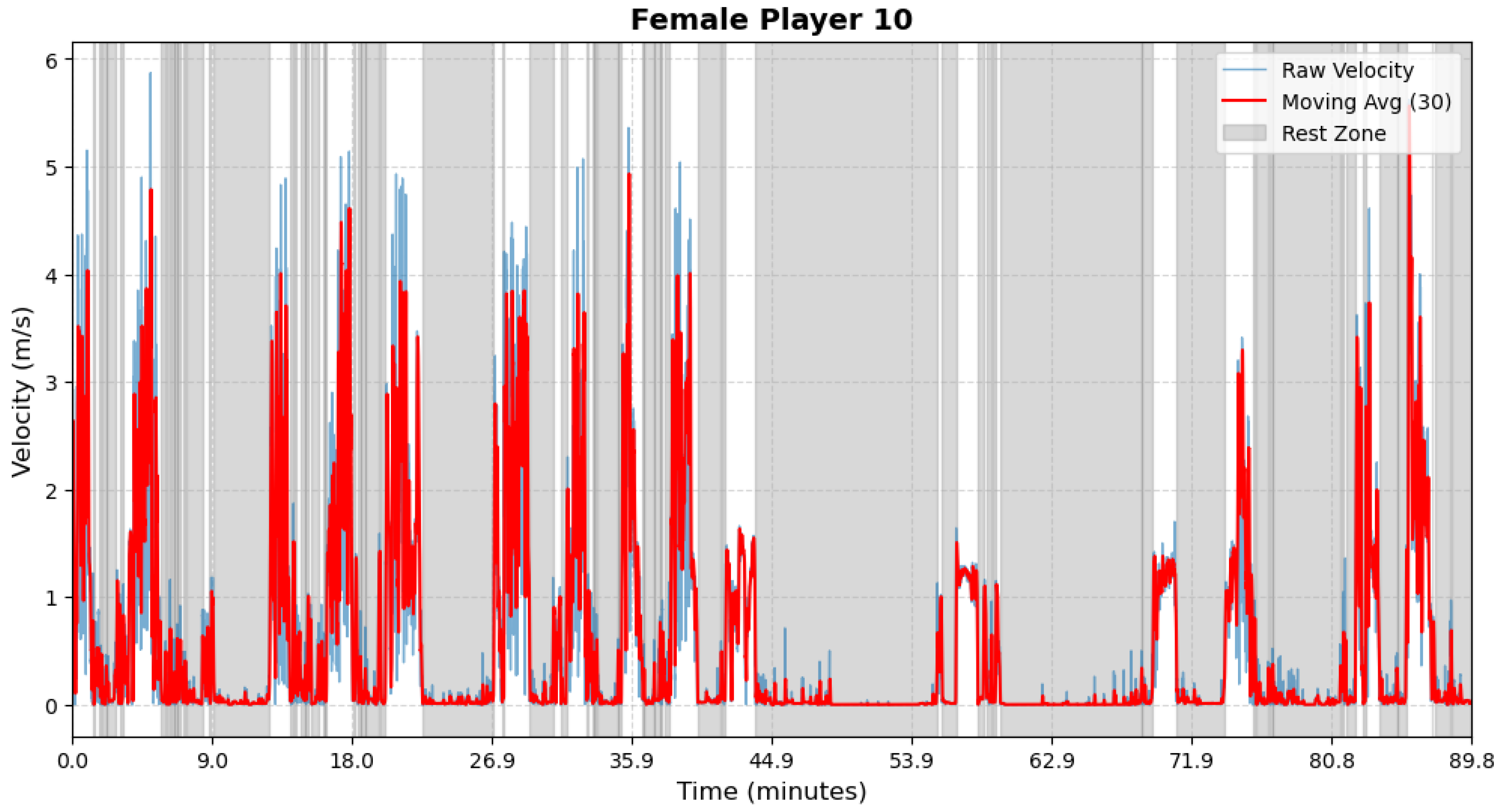
Figure A10.
Female athlete 11—Period Segmentation.
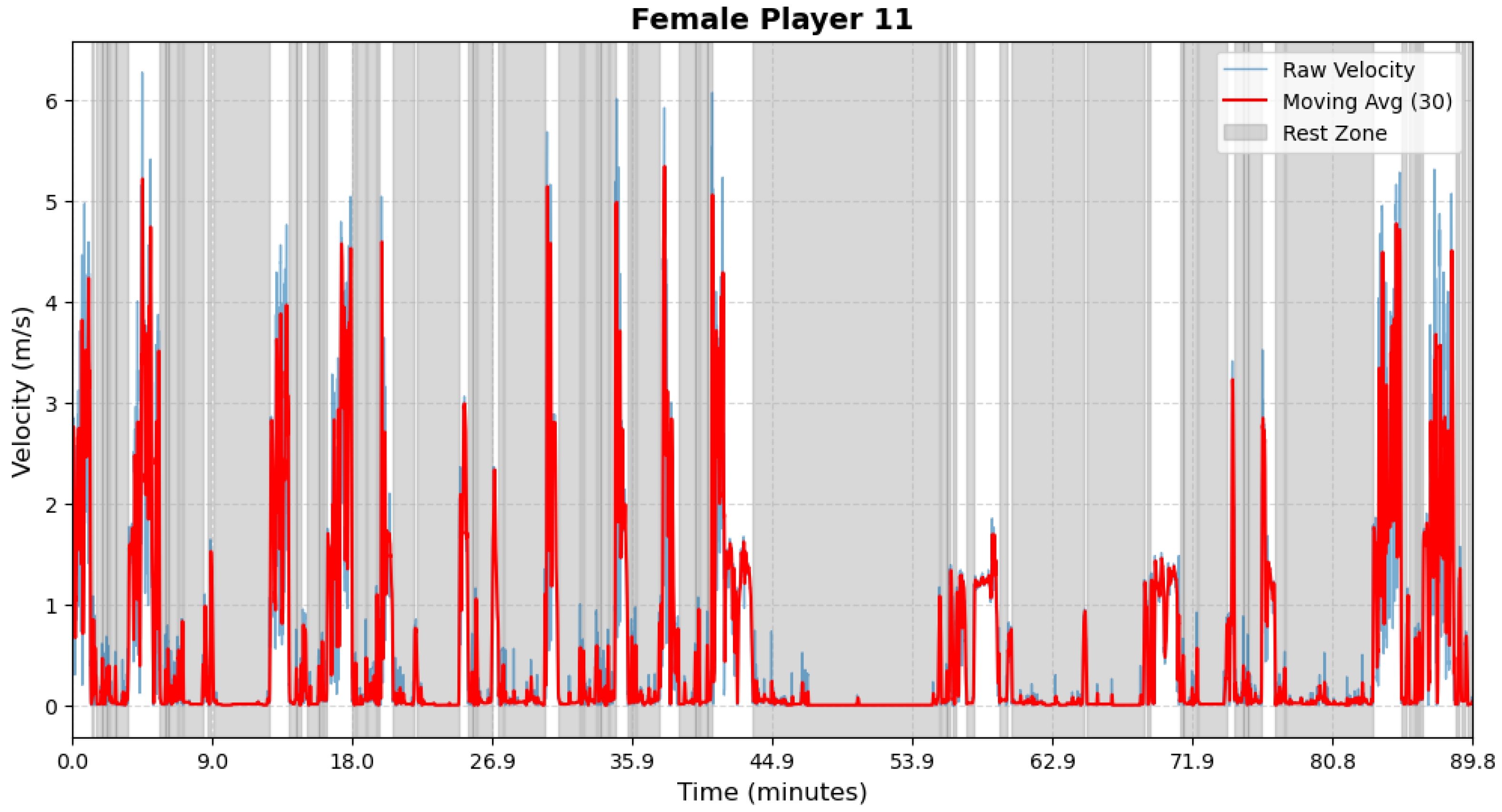
Figure A11.
Female athlete 12—Period Segmentation.
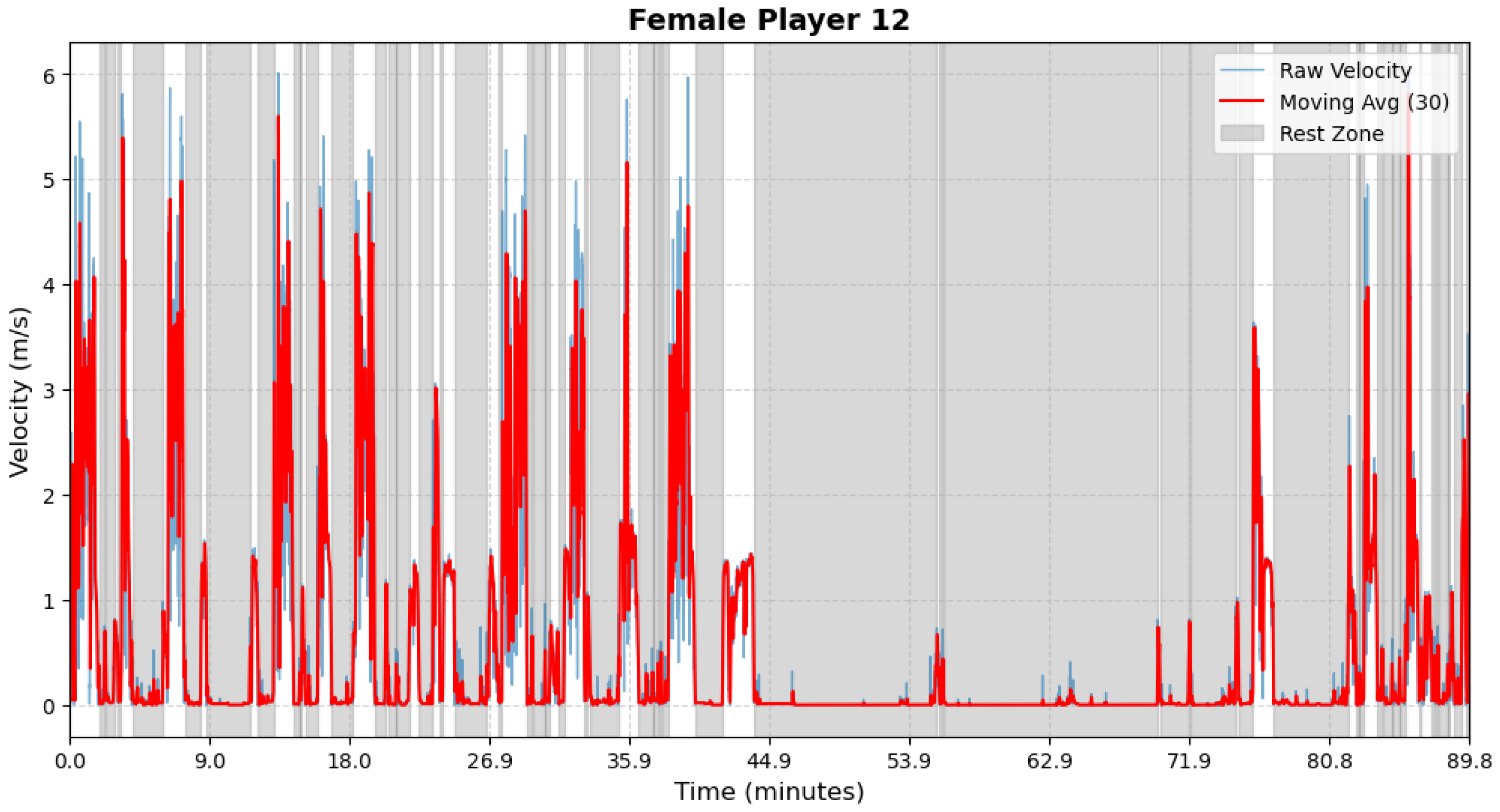
Figure A12.
Male athlete 3—Period Segmentation.
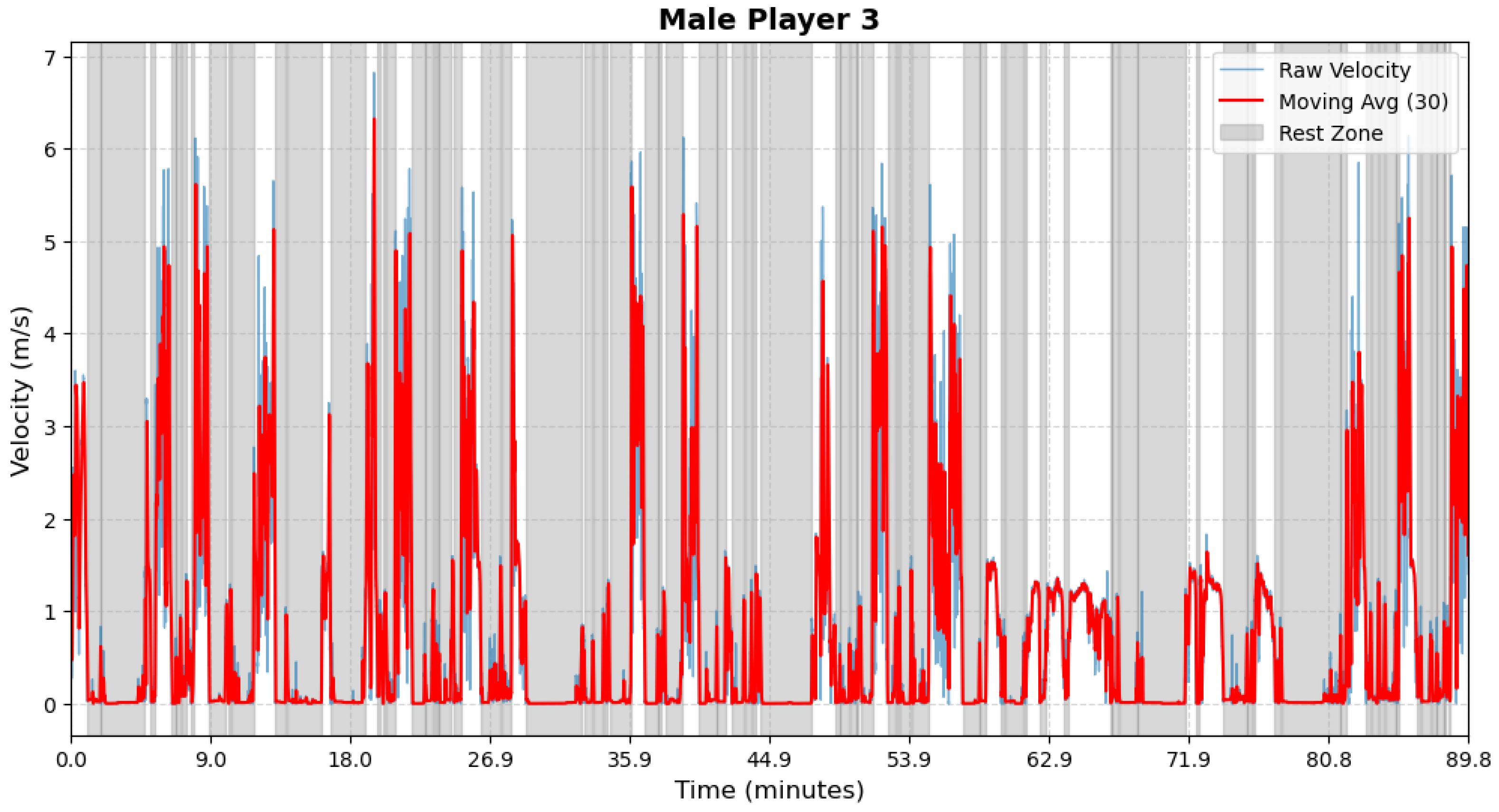
Figure A13.
Male athlete 4—Period Segmentation.
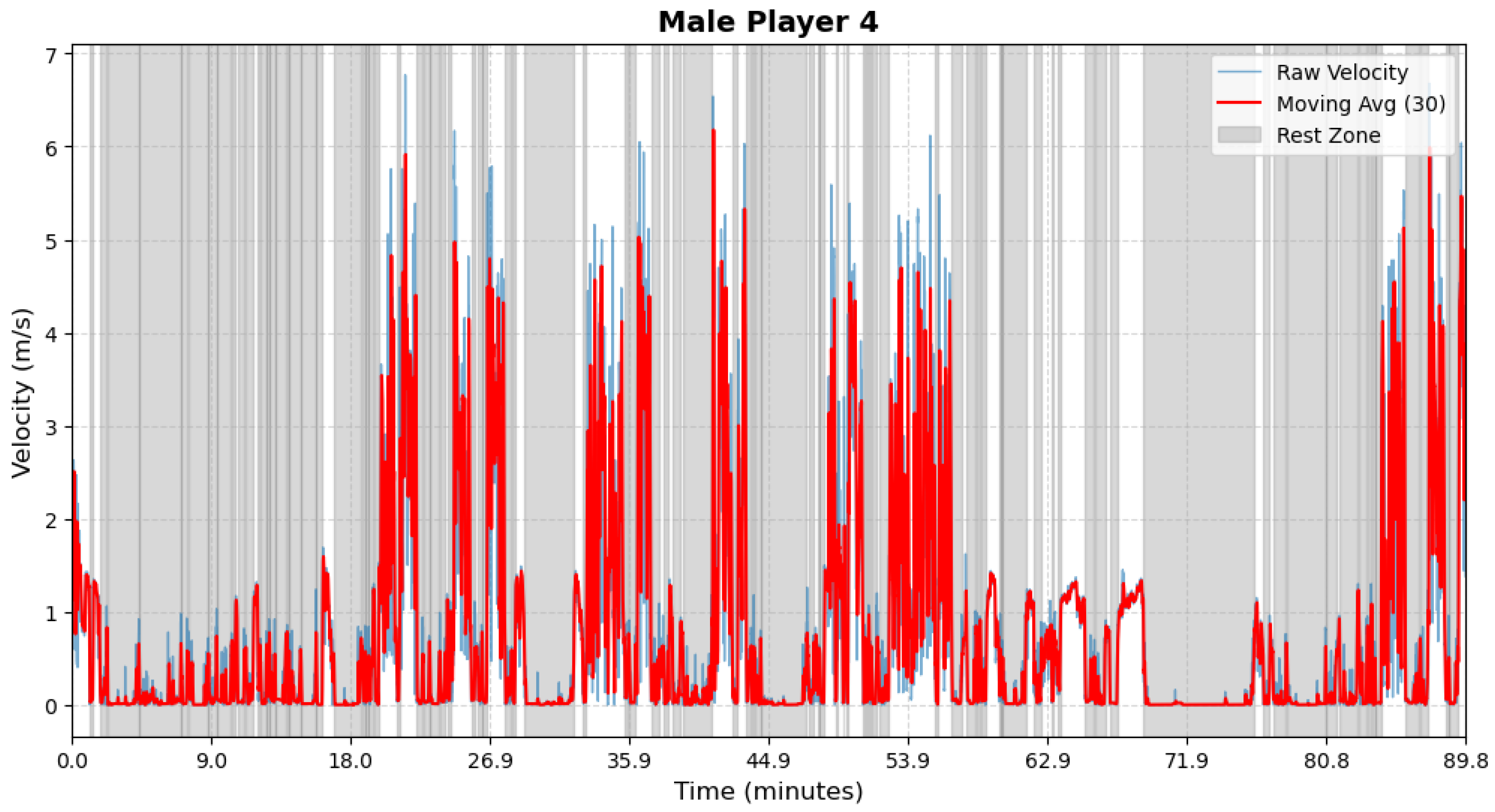
Figure A14.
Male athlete 5—Period Segmentation.
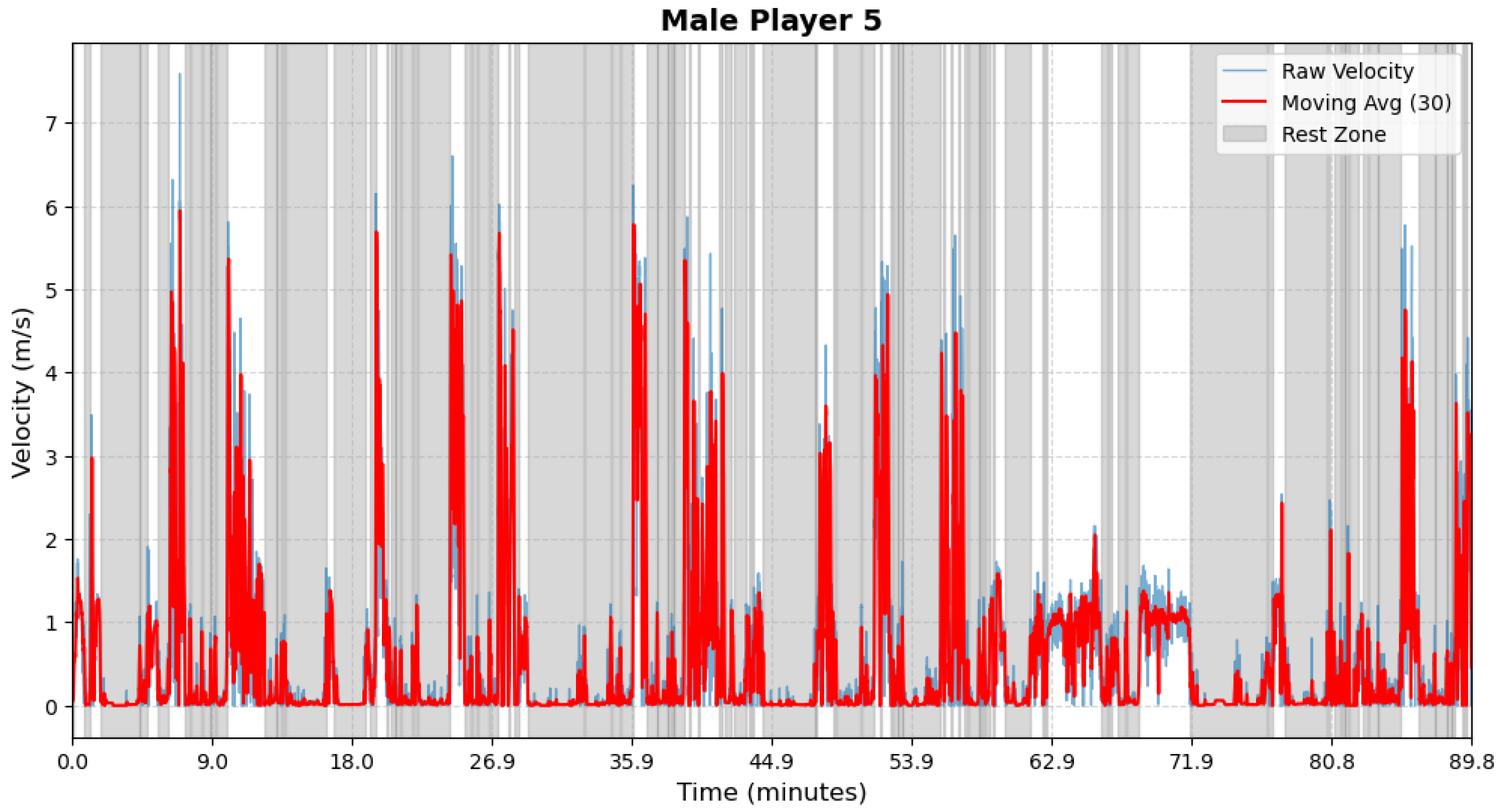
Figure A15.
Male athlete 6—Period Segmentation.
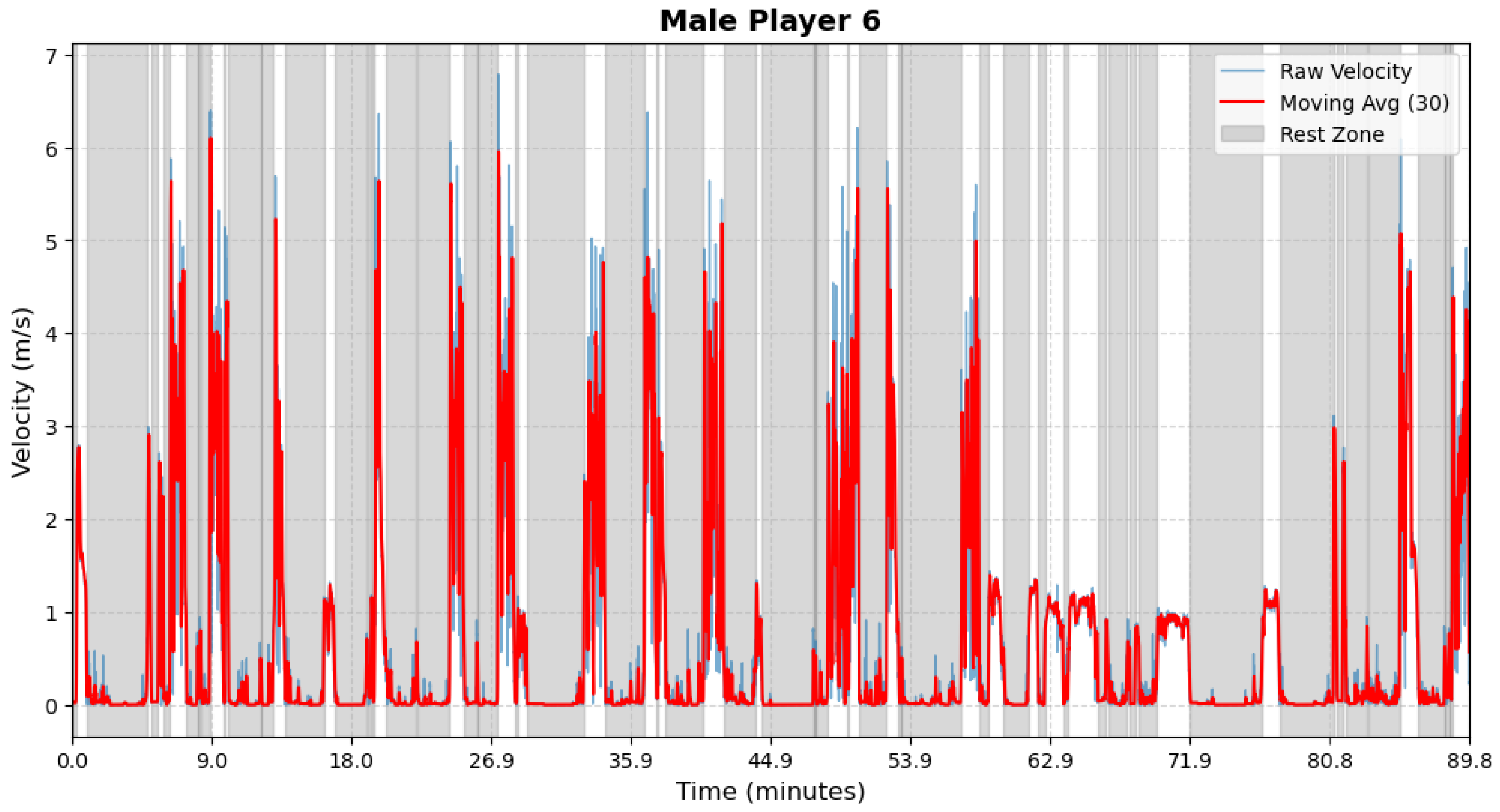
Figure A16.
Male athlete 7—Period Segmentation.
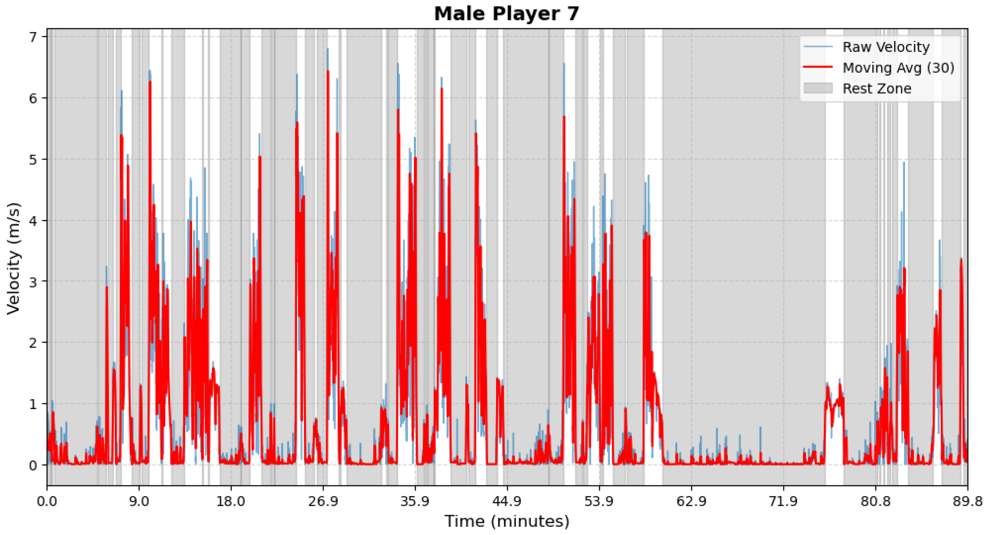
Figure A17.
Male athlete 8—Period Segmentation.
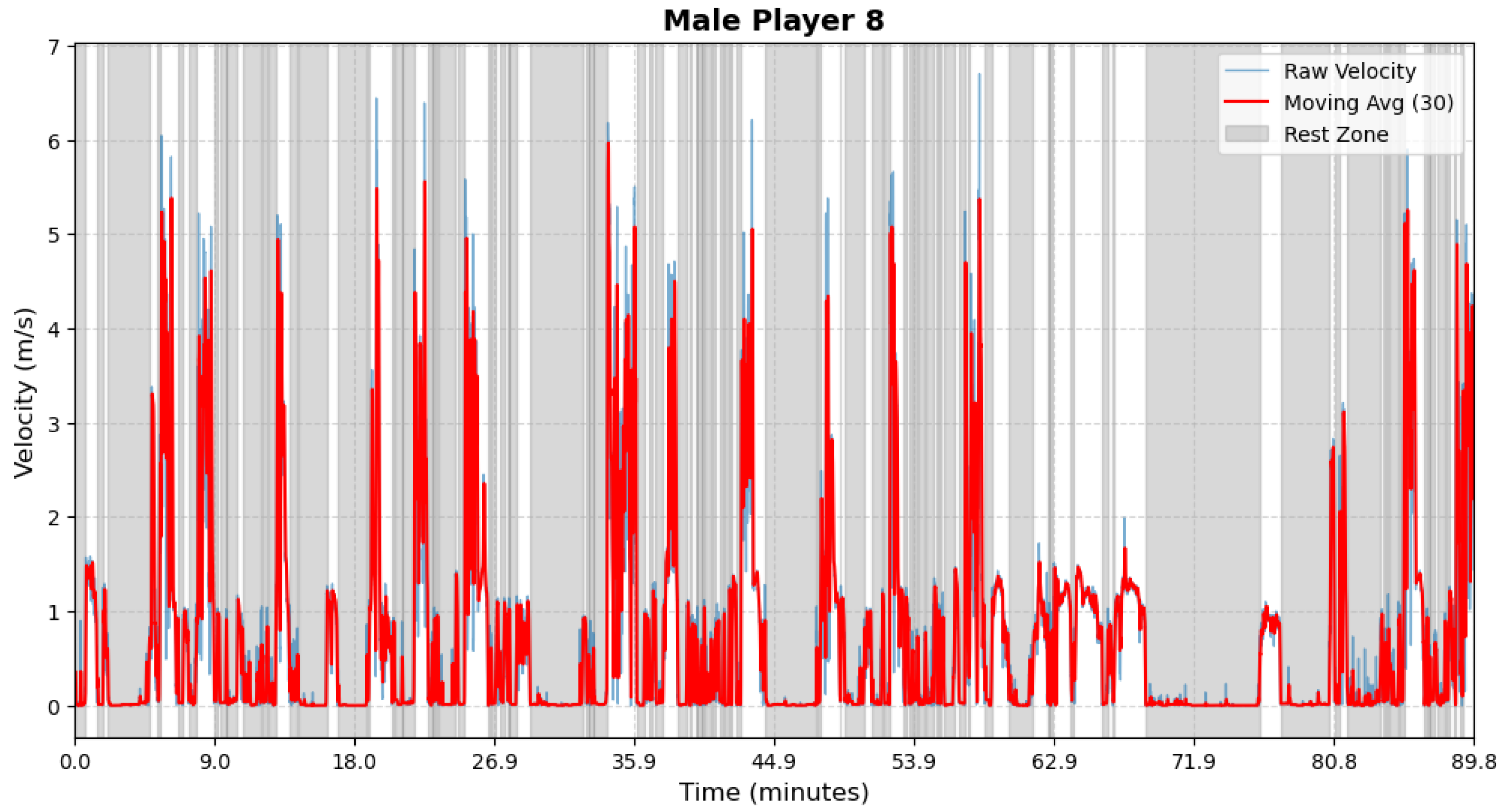
Figure A18.
Male athlete 9—Period Segmentation.
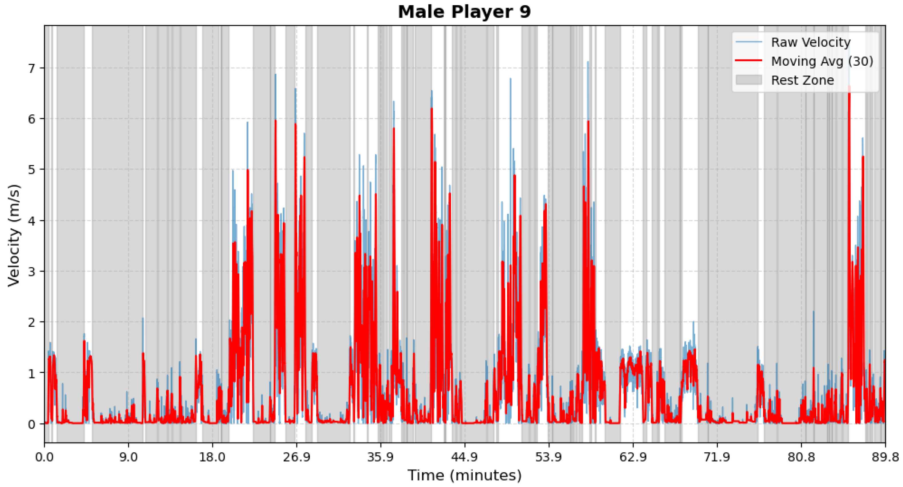
Figure A19.
Male athlete 10—Period Segmentation.
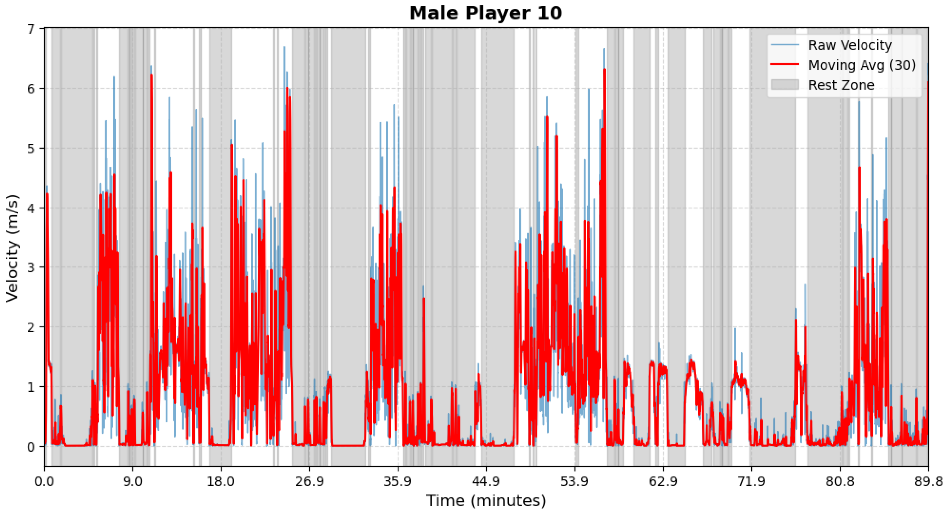
Figure A20.
Male athlete 11—Period Segmentation.
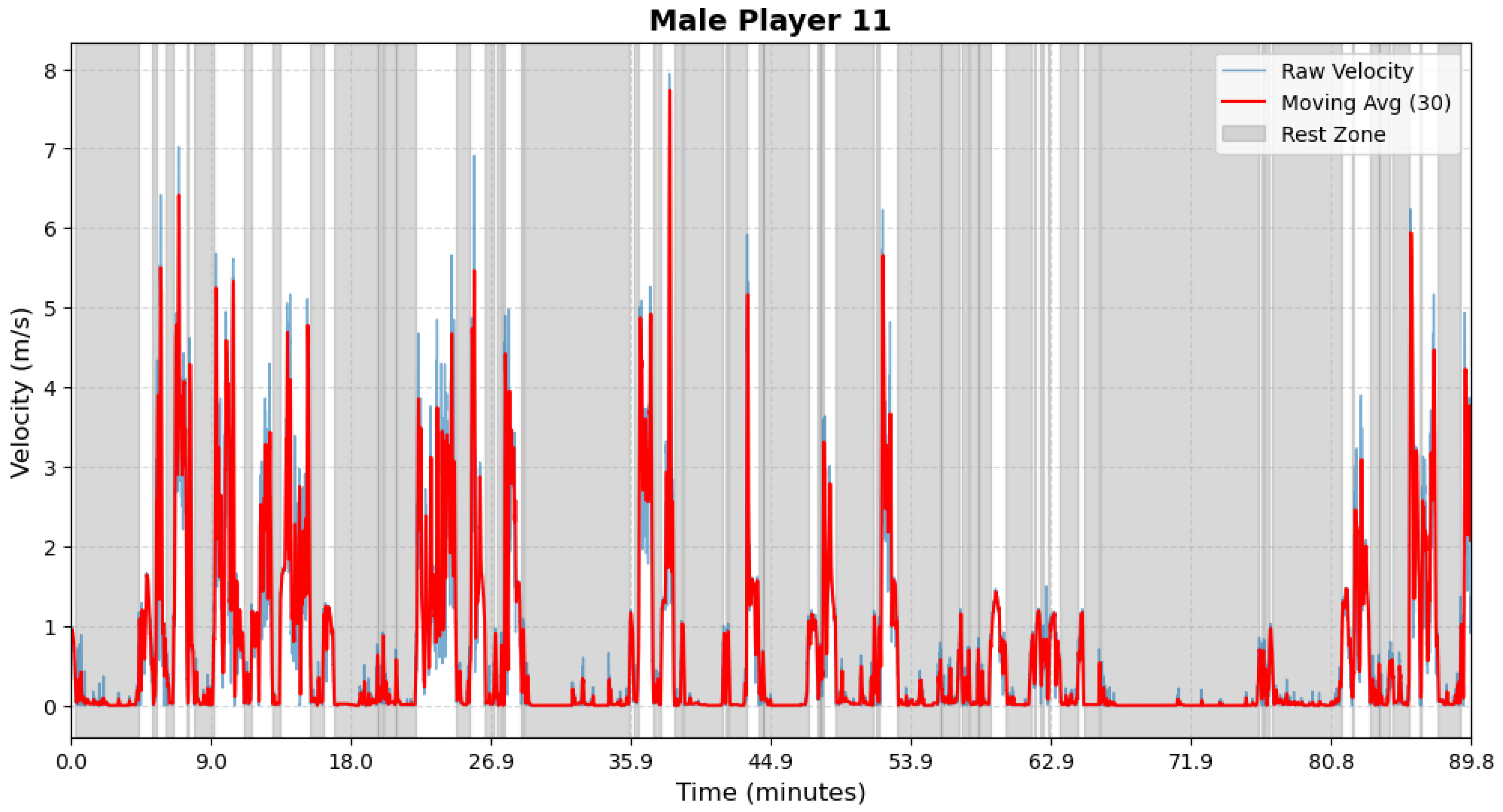
Figure A21.
Male athlete 12—Period Segmentation.
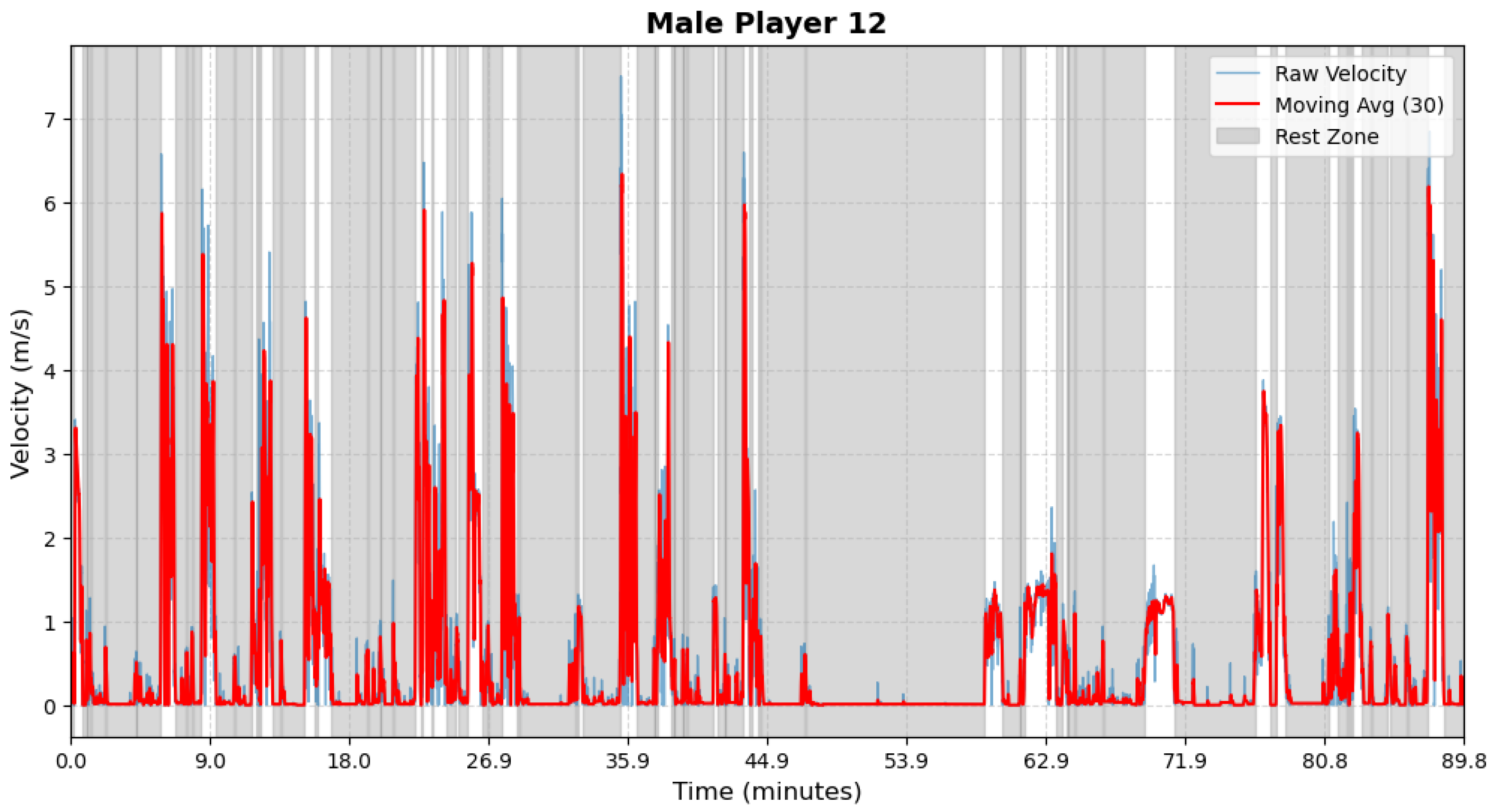
Figure A22.
Male athlete 13—Period Segmentation.
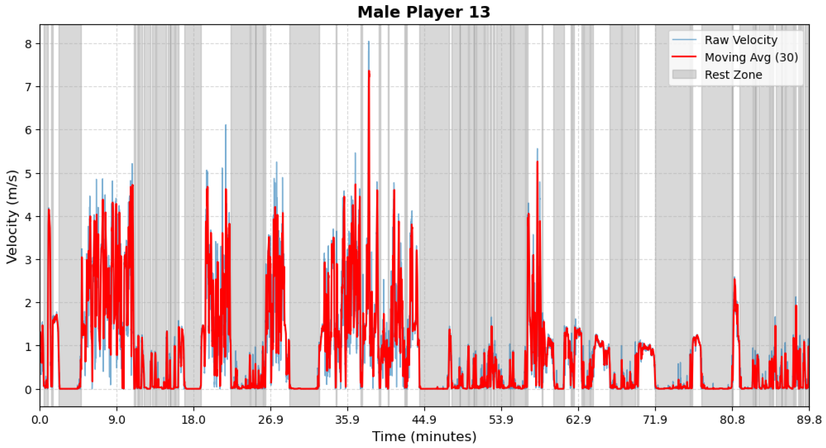
Figure A23.
Male athlete 14—Period Segmentation.
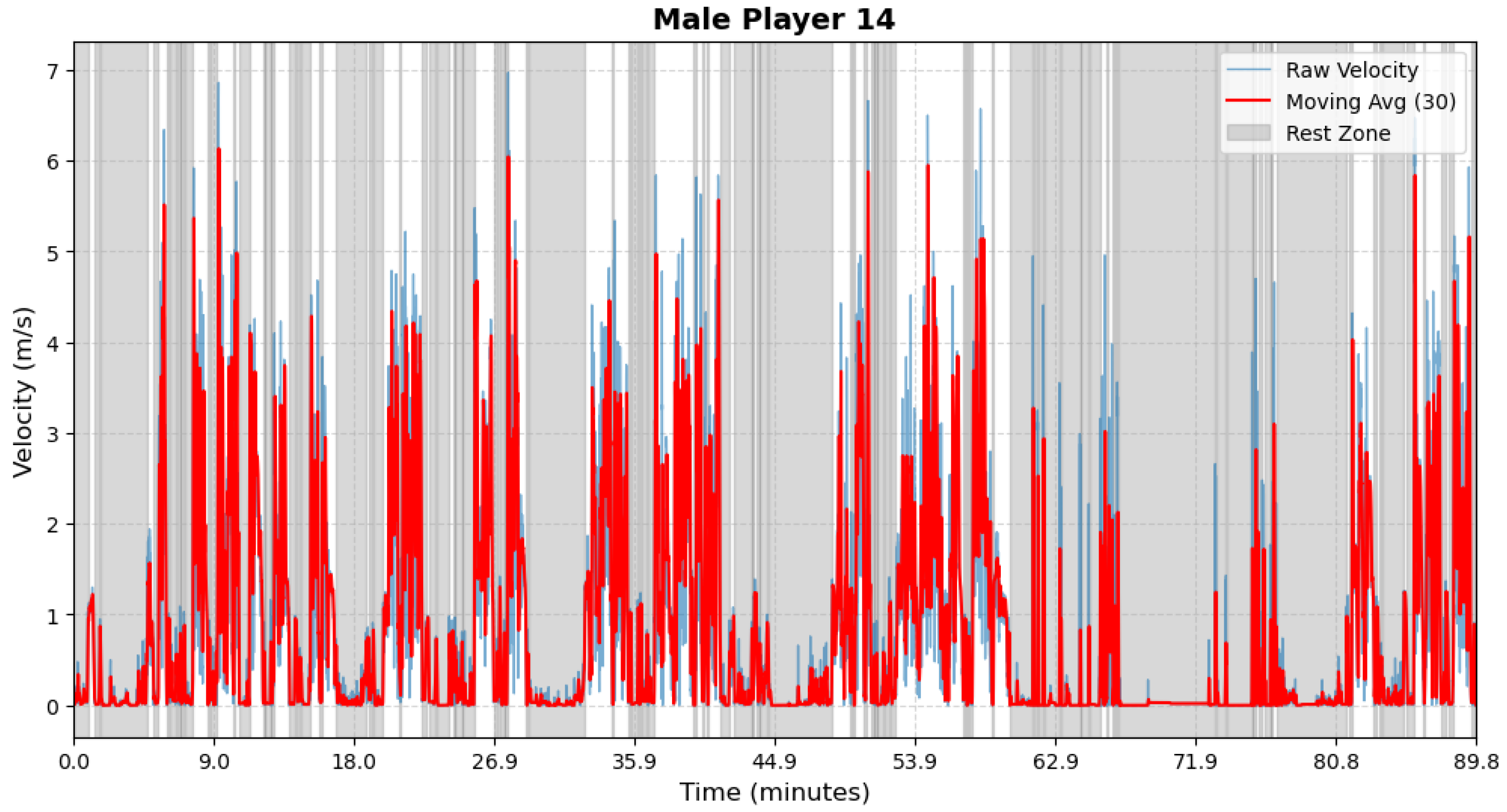
Figure A24.
Male athlete 15—Period Segmentation.
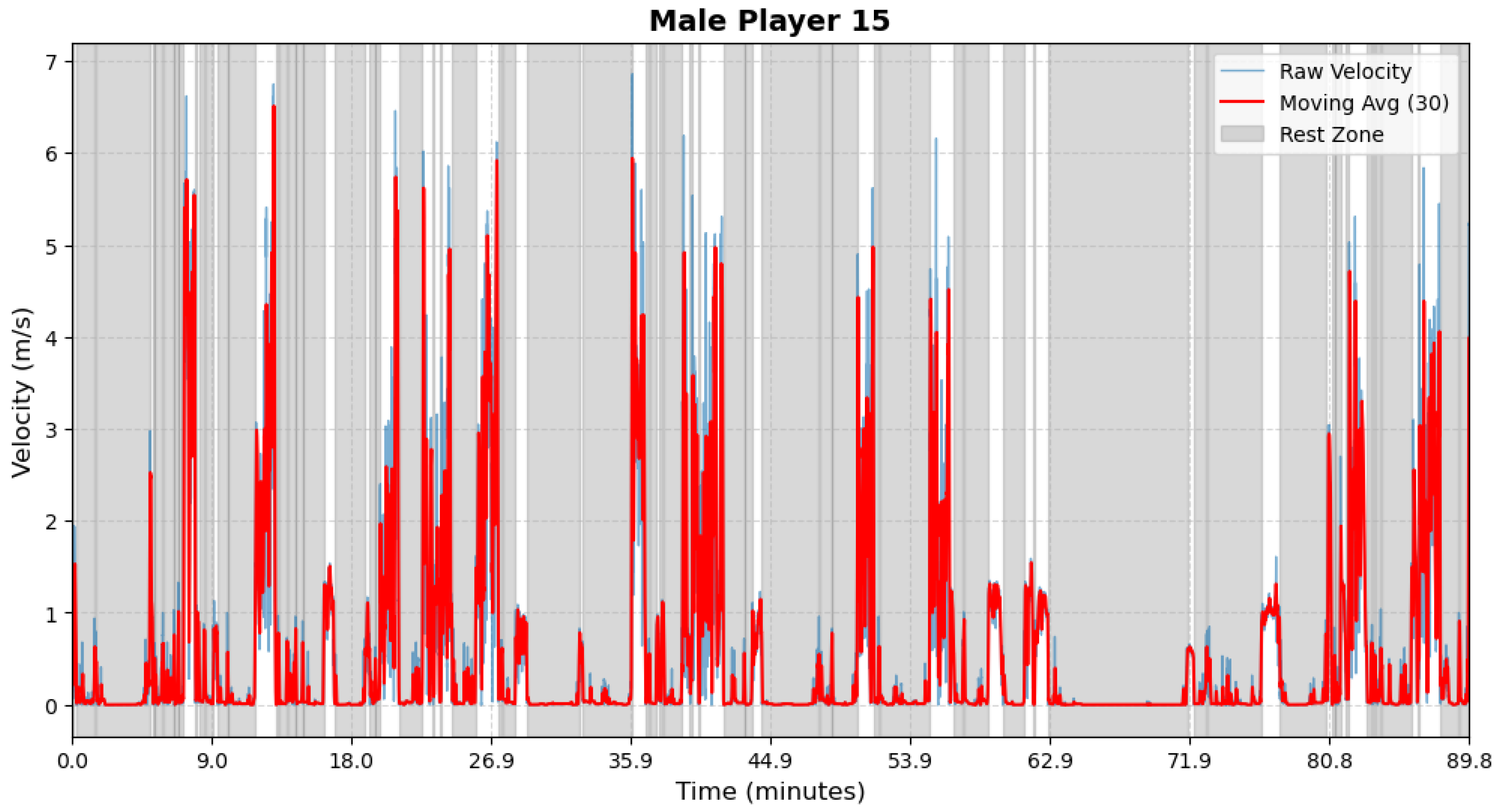
Appendix C. Gamma Distribution for Frailty Term
To further investigate the impact of the frailty term in our model, we allow our framework by incorporating a Gamma distribution into the frailty component, which allows for a skew distribution and provides greater flexibility in capturing unobserved heterogeneity. However, the PAMM framework does not support the incorporation of Gamma distribution into the frailty term. Therefore, we have to adopt a Bayesian approach using Markov Chain Monte Carlo sampling to estimate the model parameters. The FM and TSFM models with Gamma distribution are referred to as FMG and TSFMG, respectively. In these models, the Gamma distribution is assumed to have mean 1 and variance . The estimated model parameters are presented in Table A1. We then compare the model performance in terms of AIC, AUC(t), and iAUC. According to Table A2, Table 4 and Table 5, we found that the model performance did not improve further. This may be due to the small sample size; further investigation with a larger dataset is needed, but we leave it for future research.
Table A1.
Parameter Estimates.
Table A2.
Model Performance Evaluation.
References
- Federation of International Touch. FIT Playing Rules of Touch, 5th ed.; Federation of International Touch: Melbourne, Australia, 2020; Available online: https://www.internationaltouch.org/what-is-touch/the-rules/rules-of-the-game/ (accessed on 1 March 2026).
- Cropper, E.; Thorpe, C.; Roberts, S.; Twist, C. Injury Surveillance during a European Touch Rugby Championship. Sports 2019, 7, 71. [Google Scholar] [CrossRef] [Scilit] [PubMed]
- Fuller, C.; Ashton, T.; Brooks, J.; Cancea, R.; Hall, J.; Kemp, S. Injury risks associated with tackling in rugby union. Br. J. Sport. Med. 2010, 44, 159–167. [Google Scholar] [CrossRef] [Scilit]
- Johnston, R.; Watsford, M.; Pine, M.; Spurrs, A.; Murphy, A.; Pruyn, E. The Validity and reliability of 5-hz global positioning system units to measure team sport movement demands. J. Strength Cond. Res. 2012, 26, 758–765. [Google Scholar] [CrossRef] [Scilit] [PubMed]
- Seçkin, A.; Ateş, B.; Seckin, M. Review on wearable technology in sports: Concepts, challenges and opportunities. Appl. Sci. 2023, 13, 10399. [Google Scholar] [CrossRef] [Scilit]
- Zadeh, A.; Taylor, D.; Bertsos, M.; Tillman, T.; Nosoudi, N.; Bruce, S. Predicting sports injuries with wearable technology and data analysis. Front. Physiol. 2020, 23, 1023–1037. [Google Scholar] [CrossRef] [Scilit]
- Ferraz, A.; Duarte-Mendes, P.; Sarmento, H.; Valente-Dos-Santos, J.; Travassos, B. Tracking devices and physical performance analysis in team sports: A comprehensive framework for research—trends and future directions. Front. Sport. Act. Living 2023, 5, 1284086. [Google Scholar] [CrossRef] [Scilit]
- di Prampero, P.; Fusi, S.; Sepulcri, L.; Morin, J.; Belli, A.; Antonutto, G. Sprint running: A new energetic approach. J. Exp. Biol. 2005, 208, 2809–2816. [Google Scholar] [CrossRef] [Scilit]
- Impellizzeri, F.; Marcora, S.; Coutts, A. Internal and external training load: 15 years on. Int. J. Sport. Physiol. Perform. 2019, 14, 270–273. [Google Scholar] [CrossRef] [Scilit] [PubMed]
- Martorelli, A.; De Lima, F.; Vieira, A.; Tufano, J.; Ernesto, C.; Boullosa, D.; Bottaro, M. The interplay between internal and external load parameters during different strength training sessions in resistance-trained men. Eur. J. Sport Sci. 2020, 21, 16–25. [Google Scholar] [CrossRef] [Scilit]
- Piedra, A.; Caparrós, T.; Vicens-Bordas, J.; Peña, J. Internal and external load control in team sports through a multivariable model. J. Sport. Sci. Med. 2021, 20, 751–758. [Google Scholar] [CrossRef] [Scilit]
- Beaven, R.; Highton, J.; Thorpe, M.; Knott, E.; Twist, C. Movement and physiological demands of international and regional men’s touch rugby matches. J. Strength Cond. Res. 2014, 28, 3274–3279. [Google Scholar] [CrossRef] [Scilit] [PubMed]
- Cummins, C.; Orr, R.; O’Connor, H.; West, C. Global positioning systems (GPS) and microtechnology sensors in team sports: A systematic review. Sport. Med. 2013, 43, 1025–1042. [Google Scholar] [CrossRef] [Scilit]
- Hausler, J.; Halaki, M.; Orr, R. Application of Global Positioning System and Microsensor Technology in Competitive Rugby League Match-Play: A Systematic Review and Meta-analysis. Sport. Med. 2016, 46, 559–588. [Google Scholar] [CrossRef] [Scilit]
- Jennings, D.; Cormack, S.; Coutts, A.; Boyd, L.; Aughey, R. The validity and reliability of GPS units for measuring distance in team sport specific running patterns. Int. J. Sport. Physiol. Perform. 2010, 5, 328–341. [Google Scholar] [CrossRef] [Scilit] [PubMed]
- Varley, M.; Fairweather, I.; Aughey, R.J. Validity and reliability of GPS for measuring instantaneous velocity during acceleration, deceleration, and constant motion. J. Sport. Sci. 2012, 30, 121–127. [Google Scholar] [CrossRef] [Scilit]
- Johnston, R.; Watsford, M.; Kelly, S.; Pine, M.; Spurrs, R. Validity and interunit reliability of 10 Hz and 15 Hz GPS units for assessing athlete movement demands. J. Strength Cond. Res. 2014, 28, 1649–1655. [Google Scholar] [CrossRef] [Scilit]
- Nikolaidis, P.; Clemente, F.; van der Linden, C.; Rosemann, T.; Knechtle, B. Validity and reliability of 10-hz global positioning system to assess in-line movement and change of direction. Front. Physiol. 2018, 9, 228. [Google Scholar] [CrossRef] [Scilit]
- Chow, C. Global positioning system activity profile in touch rugby: Does training meet the match-play intensity in a two-day international test match series? J. Sport. Sci. Med. 2020, 19, 613. [Google Scholar]
- Vickery, W.; Harkness, A. Physical, physiological and perceptual match demands of amateur mixed gender touch players. J. Sport. Sci. Med. 2017, 16, 589. [Google Scholar]
- Zaragoza, J.; Prather, J.; Florez, C.; Goonan, J.; Tinnin, M.; Secrest, A.; Taylor, L.; Elsworthy, N.; Dalbo, V. 2019 Touch World Cup: An analysis of movement demands by half and gender. Int. J. Sport. Sci. Coach. 2023, 18, 1240–1247. [Google Scholar] [CrossRef] [Scilit]
- Nielsen, R.O.; Bertelsen, M.L.; Ramskov, D.; Møller, M.; Hulme, A.; Theisen, D.; Finch, C.F.; Fortington, L.V.; Mansournia, M.A.; Parner, E.T. Time-to-event analysis for sports injury research part 2: Time-varying outcomes. Br. J. Sport. Med. 2019, 53, 70–78. [Google Scholar] [CrossRef] [Scilit]
- Halson, S. Monitoring Training Load to Understand Fatigue in Athletes. Sport. Med. 2014, 44, 139–147. [Google Scholar] [CrossRef] [Scilit] [PubMed]
- Windt, J.; Gabbett, T. How do training and competition workloads relate to injury? The workload—injury aetiology model. Br. J. Sport. Med. 2017, 51, 428–435. [Google Scholar] [CrossRef] [Scilit]
- Griffin, A.; Kenny, I.; Comyns, T.; Lyons, M. The association between the acute:chronic workload ratio and injury and its application in team sports: A systematic review. Sport. Med. 2020, 50, 561–580. [Google Scholar] [CrossRef] [Scilit]
- Taylor, R.; Myers, T.; Sanders, D.; Ellis, M.; Akubat, I. The Relationship between Training Load Measures and Next-Day Well-Being in Rugby Union Players. Appl. Sci. 2021, 11, 5926. [Google Scholar] [CrossRef] [Scilit]
- Foster, C.; Florhaug, J.; Franklin, J.; Gottschall, L.; Hrovatin, L.; Parker, S.; Doleshal, P.; Dodge, C. A new approach to monitoring exercise training. J. Strength Cond. Res. 2001, 15, 109–115. [Google Scholar]
- Hulin, B.; Gabbett, T.; Lawson, D.; Caputi, P.; Sampson, J. The acute: Chronic workload ratio predicts injury: High chronic workload may decrease injury risk in elite rugby league players. Br. J. Sport. Med. 2016, 50, 231–236. [Google Scholar] [CrossRef] [Scilit]
- Akenhead, R.; Nassis, G. Training load and player monitoring in high-Level football: Current practice and perceptions. Int. J. Sport. Physiol. Perform. 2016, 11, 587–593. [Google Scholar] [CrossRef] [Scilit] [PubMed]
- Hader, K.; Rumpf, M.; Hertzog, M.; Kilduff, L.; Girard, O.; Silva, J. Monitoring the athlete match response: Can external load variables predict post-match acute and residual fatigue in soccer? A systematic review with meta-analysis. Sport. Med. 2019, 5, 48. [Google Scholar] [CrossRef] [Scilit]
- Kaplan, E.; Meier, P. Nonparametric estimation from incomplete observations. J. Am. Stat. Assoc. 1958, 53, 457–481. [Google Scholar] [CrossRef]
- Mantel, N. Evaluation of survival data and two new rank order statistics arising in its consideration. Cancer Chemother. Rep. 1966, 50, 163–170. [Google Scholar] [PubMed]
- Cox, D. Regression models and life-tables. J. R. Stat. Soc. Ser. B (Methodol.) 1972, 34, 187–202. [Google Scholar] [CrossRef] [Scilit]
- Gabbe, B.; Finch, C.; Bennell, K.; Wajswelner, H. Risk factors for hamstring injuries in community level Australian football. Br. J. Sport. Med. 2005, 39, 106–110. [Google Scholar] [CrossRef] [Scilit]
- Yadav, C.; Sreenivas, V.; Khan, M.; Pandey, R. An overview of statistical models for recurrent events analysis: A review. Epidemiology 2018, 8, 354. [Google Scholar] [CrossRef]
- Bieszk-Stolorz, B. Relationship between coefficients in parametric survival models for exponentially distributed survival time—registered unemployment in Poland. Econometrics 2025, 13, 1. [Google Scholar] [CrossRef] [Scilit]
- Mahmood, A.; Ullah, S.; Finch, C. Application of survival models in sports injury prevention research: A systematic review. Br. J. Sport. Med. 2014, 48, 630. [Google Scholar] [CrossRef] [Scilit]
- Donaldson, M.; Sobolev, B.; Cook, W.; Janssen, P.; Khan, K. Analysis of recurrent events: A systematic review of randomised controlled trials of interventions to prevent falls. Age Ageing 2009, 38, 151–155. [Google Scholar] [CrossRef] [Scilit]
- Ozga, A.; Kieser, M.; Rauch, G. A systematic comparison of recurrent event models for application to composite endpoints. BMC Med. Res. Methodol. 2018, 18, 2. [Google Scholar] [CrossRef] [Scilit]
- Anderson, P.; Gill, R. Cox’s Regression Model for Counting Processes: A Large Sample Study. Ann. Stat. 1982, 10, 1100–1120. [Google Scholar] [CrossRef] [Scilit]
- Venturelli, M.; Schena, F.; Zanolla, L.; Bishop, D. Injury risk factors in young soccer players detected by a multivariate survival model. J. Sci. Med. Sport 2011, 14, 293–298. [Google Scholar] [CrossRef] [Scilit] [PubMed]
- Prentice, R.; Williams, B.; Peterson, A. On the regression analysis of multivariate failure time data. Biometrika 1981, 68, 373–379. [Google Scholar] [CrossRef]
- Ullah, S.; Gabbett, T.; Finch, C. Statistical modelling for recurrent events: An application to sports injuries. Br. J. Sport. Med. 2014, 48, 1287–1293. [Google Scholar] [CrossRef] [Scilit] [PubMed]
- Vaupel, J.; Manton, K.; Stallard, E. The impact of heterogeneity in individual frailty on the dynamics of mortality. Demography 1979, 16, 439–454. [Google Scholar] [CrossRef] [Scilit]
- Balan, T.A.; Putter, H. A tutorial on frailty models. Stat. Methods Med. Res. 2020, 29, 3424–3454. [Google Scholar] [CrossRef] [Scilit]
- Clayton, D. A model for association in bivariate life tables and its application in epidemiological studies of familial tendency in chronic disease incidence. Biometrika 1978, 65, 141–151. [Google Scholar] [CrossRef]
- Oakes, D. A model for association in bivariate survival data. J. R. Stat. Soc. Ser. B Stat. Methodol. 1982, 44, 414–422. [Google Scholar] [CrossRef] [Scilit]
- Macis, A. The role of the frailty in the evaluation of injury risk factors for National Basketball Association players. Comput. Stat. 2025, 40, 1985–2003. [Google Scholar] [CrossRef] [Scilit]
- Bowen, L.; Gross, A.; Gimpel, M.; Bruce-Low, S.; Li, F. Spikes in acute:chronic workload ratio (ACWR) associated with a 5-7 times greater injury rate in English Premier League football players: A comprehensive 3-year study. Br. J. Sport. Med. 2019, 54, 731–738. [Google Scholar] [CrossRef] [Scilit]
- Xu, J.; Kalbfleisch, J.; Tai, B. Statistical Analysis of Illness–Death Processes and Semicompeting Risks Data. Biometrics 2010, 66, 716–725. [Google Scholar] [CrossRef] [Scilit] [PubMed]
- Keiding, N.; Andersen, P.; Klein, J. The role of frailty models and accelerated failure time models in describing heterogeneity due to omitted covariates. Stat. Med. 1997, 66, 215–224. [Google Scholar] [CrossRef]
- Gabbett, T.; Ullah, S.; Finch, C. Identifying risk factors for contact injury in professional rugby league players—Application of a frailty model for recurrent injury. J. Sci. Med. Sport 2012, 15, 496–504. [Google Scholar] [CrossRef] [Scilit] [PubMed]
- Bender, A.; Groll, A.; Scheipl, F. A generalized additive model approach to time-to-event analysis. Stat. Model. 2018, 18, 299–321. [Google Scholar] [CrossRef] [Scilit]
- Simon, N.; Friedman, J.; Hastie, T.; Tibshirani, R. Regularization paths for Cox’s proportional hazards model via coordinate descent. J. Stat. Softw. 2011, 39, 1–13. [Google Scholar] [CrossRef] [Scilit] [PubMed]
- Sweeting, A.; Cormack, S.; Morgan, S.; Aughey, R. When is a sprint a sprint? A review of the analysis of team-sport athlete activity profile. Front. Physiol. 2017, 8, 432. [Google Scholar] [CrossRef] [Scilit]
- Harper, D.; Carling, C.; Kiely, J. High-Intensity acceleration and deceleration demands in elite team sports competitive match play: A systematic review and meta-analysis of observational studies. Sport. Med. 2019, 49, 1923–1947. [Google Scholar] [CrossRef] [Scilit]
- Dwyer, D.; Gabbett, T. Global positioning system data analysis: Velocity ranges and a new definition of sprinting for field sport athletes. J. Strength Cond. Res. 2012, 26, 818–824. [Google Scholar] [CrossRef] [Scilit]
- Marutani, Y.; Konda, S.; Ogasawara, I.; Yamasaki, K.; Yokoyama, T.; Maeshima, E.; Nakata, K. Gaussian mixture modeling of acceleration-derived signal for monitoring external physical load of tennis player. Front. Physiol. 2023, 14, 1161182. [Google Scholar] [CrossRef] [Scilit]
- Richardson, A.; Welsh, A. Robust restricted maximum likelihood in mixed linear models. Biometrics 1995, 51, 1429–1439. [Google Scholar] [CrossRef] [Scilit]
- Heagerty, P.; Zheng, Y. Survival model predictive accuracy and ROC curves. Biometrics 2005, 61, 92–105. [Google Scholar] [CrossRef] [Scilit]

Disclaimer/Publisher’s Note: The statements, opinions and data contained in all publications are solely those of the individual author(s) and contributor(s) and not of MDPI and/or the editor(s). MDPI and/or the editor(s) disclaim responsibility for any injury to people or property resulting from any ideas, methods, instructions or products referred to in the content. |
© 2026 by the authors. Licensee MDPI, Basel, Switzerland. This article is an open access article distributed under the terms and conditions of the Creative Commons Attribution (CC BY) license.