


Abstract
We propose an exploratory framework based on Topological Digital Twins (TDTs) for the monitoring and short-term forecasting of spatial dynamical systems. The approach represents the system through a reduced state built from topological descriptors obtained via persistent homology. These descriptors capture features such as connected components, cycles, and large-scale structure. The framework combines three components: an observation operator mapping spatial fields to a low-dimensional state, a reduced dynamical model evolving this state in time, and a data assimilation step aimed at improving robustness. This construction maps persistence diagrams to a finite-dimensional Euclidean space. This makes the model tractable but does not preserve the full algebraic structure of the original topological objects. We provide theoretical results supporting the stability of the representation under perturbations of the input field. The method is illustrated on a bow-echo convective system observed over Corsica on 18 August 2022, where the reduced state captures the main structural organization of the system over time. A comparison with standard nowcasting methods shows complementary behavior: pixel-based approaches provide better local accuracy, while the TDT framework better preserves the global spatial structure, as reflected by Wasserstein distances and persistence-based comparisons. Additional tests also indicate that the topological observables remain stable under small perturbations of the input field. The present study is based on a single case and should be understood as a proof of concept, rather than as a definitive validation. Future work will focus on validation on larger datasets and on the use of more advanced dynamical models.
Keywords:
topological digital twin; persistent homology; cubical complex; data assimilation; stability; Wasserstein distance; bow echo forecasting MSC:
55N31; 68T09; 52-08; 62M20
1. Introduction
Digital twins aim to couple mathematical models of physical systems with data streams in order to estimate, monitor, and forecast their evolution in real time. The concept, originally introduced in the context of product lifecycle management by Grieves, describes a cyber–physical architecture in which a physical system, its virtual representation, and the data connections between them interact continuously [1]. More generally, a digital twin can be viewed as a dynamic computational replica of a real system that integrates observations, models and data analytics to reproduce and predict the behavior of the physical system throughout its operational life [2,3].
Digital twins are now widely used for the monitoring and control of complex systems in engineering, geophysics, manufacturing and management. Their purpose extends beyond simulation to real-time synchronization between physical and digital entities, enabling tasks such as anomaly detection, forecasting, optimization and decision support [4]. In many applications, the state of the system is represented by high-dimensional spatial fields, such as radar reflectivity maps, satellite imagery or multiphysics simulation outputs.
In its canonical formulation, a digital twin involves a real-time, bidirectional coupling between a physical system and its digital counterpart, including feedback or control mechanisms. In the present work, we adopt a more focused and methodological perspective. In particular, the proposed framework does not implement a full cyber–physical digital twin in the canonical sense but, rather, focuses on a topology-informed representation and forecasting layer within such architectures.
The proposed Topological Digital Twin (TDT) concentrates on the observation and representation layers of such architectures. Rather than aiming at full cyber–physical coupling, it constructs a reduced-order representation of the system based on topological descriptors extracted from observational data via persistent homology. In this sense, the TDT can be viewed as a topology-driven representation layer within a broader digital twin framework.
This perspective is particularly relevant for systems described by high-dimensional spatial fields. In such settings, two main challenges arise. First, the dimension of the state space can become extremely large, making classical state estimation or reduced-order filtering methods difficult to apply without strong modeling assumptions. Second, the reliability and interpretability of the digital representation may be affected by measurement noise, missing data, or nonstationary dynamics, which are common features of observational systems.
These limitations motivate the search for alternative representations that capture the structural organization of the data while remaining robust under perturbations. In this context, a topological data analysis (TDA) offers a mathematical framework for extracting geometric and topological descriptors from complex data sets. Persistent homology, in particular, enables the identification and quantification of multiscale structures such as connected components and loops, and it benefits from well-established stability properties with respect to perturbations of the data [5,6,7]. Beyond these foundational results, significant developments have been made in recent years in both the theoretical and applied aspects of TDA. These include advances in statistical and probabilistic topological inference [8,9], scalable computational methods for large datasets [10], and the integration of topological descriptors into machine learning pipelines [11,12]. Topological methods have also been increasingly applied to dynamical systems and time-dependent data, where persistence-based descriptors are used to capture structural transitions and regime changes [13,14]. These developments highlight the growing role of TDA as a bridge between geometry, statistics, and data-driven modeling.
More structured topological frameworks, such as those based on multi-parameter persistence modules [15,16], chain-complex and homological algebra approaches [17,18], or sheaf- and category-theoretic formulations [19,20,21,22], preserve more of the underlying algebraic structure but typically lead to significantly higher computational complexity.
These alternative frameworks highlight an important distinction in the topological modeling of dynamical systems. Approaches based on multi-parameter persistence modules, chain complexes, sheaf-theoretic constructions, or categorical formalisms aim to preserve a richer part of the underlying algebraic structure. In such settings, the state space itself may retain an intrinsic topological or algebraic meaning, and the evolution is described through compatible morphisms, functorial constructions, or structured diagrammatic relations.
By contrast, the present work adopts a deliberately reduced-order perspective. The objective is not to construct a fully intrinsic topological dynamical system but to extract a finite-dimensional state from persistence-based descriptors that remains interpretable, stable under perturbations, and directly usable in a forecasting and data assimilation pipeline. This choice necessarily involves a loss of algebraic and combinatorial structure after vectorization, but it makes the resulting representation tractable for numerical modeling and for comparison with standard reduced-order forecasting methods.
In this sense, the proposed framework should be viewed as complementary to more structured topological approaches, rather than as a substitute for them. Richer frameworks may preserve more information and offer a deeper intrinsic description of topological evolution, but they also typically lead to a substantially higher level of mathematical and computational complexity. The present study focuses instead on the question of whether topological observables can serve as stable and useful reduced states for short-term prediction and assimilation in a concrete applied setting.
Within this setting, the Topological Digital Twin represents the system through the evolution of a reduced topological state derived from observational data streams. Persistent homology maps complex spatial fields to low-dimensional yet structurally meaningful descriptors, which remain stable under perturbations. This reduced representation provides a tractable state suitable for dynamical modeling and data assimilation, at the cost of not preserving the full algebraic structure of the underlying topological objects.
We outline the main elements of the framework, analyze its stability properties, and illustrate its relevance on the forecasting of convective bow-echo systems from radar observations. The present work should be understood as an exploratory study whose objective is to introduce and assess the Topological Digital Twin framework on a representative case, rather than to provide a fully general or operational solution. The contribution is, therefore, primarily methodological, and it focuses on the integration of existing topological stability results within a reduced-order dynamical and data assimilation framework.
Topological Data Analysis offers a complementary viewpoint: rather than forecasting each pixel value, one tracks global geometric and topological structures such as connectivity, loops, cavities or mesoscale patterns encoded by persistent homology [23,24]. For spatial fields defined on regular grids (e.g., radar reflectivity maps), these structures can be extracted through cubical filtrations. The resulting persistence diagrams summarize the multiscale topology of the field and capture structural transitions, such as the merging of clusters, the formation of arcs, or the appearance of holes.
Persistent homology and its stability properties are well established [5,25]. Vectorization techniques such as persistence landscapes and persistence images enable the integration of topological descriptors into statistical learning pipelines [26,27,28]. However, mapping persistence diagrams to finite-dimensional vectors induces a loss of algebraic and combinatorial structure. This transformation corresponds to a transition from intrinsically topological objects to a Euclidean representation. This transition involves a trade-off between structural fidelity and computational tractability. While part of the algebraic and categorical information carried by persistence diagrams is lost after vectorization, the resulting representation enables the definition of stable and computationally efficient dynamical models compatible with standard forecasting and data assimilation techniques.
This choice is motivated by the need to define a tractable dynamical model and to enable data assimilation in a Euclidean setting. In particular, standard forecasting and assimilation tools rely on vector space structures that are not directly available at the level of persistence diagrams.
On the data assimilation side, Kalman filtering and ensemble-based methods form the standard toolbox [29,30]. Optimal transport plays a key role in the comparison of persistence diagrams, notably through Wasserstein distances [31]. In computer vision, optical flow methods provide simple advection models frequently used as baselines for short-term forecasting [32,33].
Our contribution is to connect these components within a unified Topological Digital Twin framework. The proposed framework aims to bridge topological data analysis, dynamical systems, and data assimilation in a unified and interpretable setting. It should be understood as a hybrid construction, where topological descriptors inform the state representation, while the evolution is governed by a reduced dynamical model in a Euclidean space. We introduce a reduced dynamical state built from topological observables, analyze its stability under perturbations of the observed field, and illustrate the resulting pipeline on a severe convection radar case study.
From a dynamical perspective, this approach represents the evolution of a spatial system through the trajectory of a reduced state derived from topological descriptors see Figure 1. Instead of evolving a high-dimensional field, one studies the dynamics of a low-dimensional representation that captures the structural organization of the system across scales.
Figure 1.
Pipeline of a Topological Digital Twin. The observed spatial field, , is transformed into a cubical filtration, from which a persistence diagram, , is computed. A topological observation operator, , maps the diagram to a finite-dimensional state vector, . The internal dynamics, , evolves this Euclidean reduced state, while the assimilation operator, , incorporates new observations.
It is important to note that, due to the vectorization step, the state lies in a Euclidean space and does not retain the full algebraic structure of the underlying persistence diagrams. The resulting dynamics should, therefore, be understood as a topology-informed reduced-order evolution, rather than as fully intrinsic topological dynamics.
Bow-echo systems are organized convective structures associated with damaging straight-line winds and strong mesoscale organization. Their radar signatures typically exhibit a curved convective line, rear-inflow jets, and evolving internal vortices, often accompanied by bookend vortices and mesoscale convective system dynamics [34,35,36,37]. Such systems frequently produce widespread severe winds and occasionally tornadoes, making their detection and monitoring a major operational challenge in severe weather forecasting.
From a geometric standpoint, these patterns correspond to evolving arcs and holes in reflectivity superlevel sets, reflecting the bow-shaped convective line and the development of rear-inflow notches or embedded circulation features. Persistent homology, therefore, yields a natural mathematical descriptor for capturing the structural organization and evolution of these mesoscale patterns [38,39].
At the same time, radar products contain structured artifacts such as no-data sectors, radial wedges, attenuation zones, or missing scans arising from the acquisition geometry and signal processing pipeline. Pixel-wise learning approaches may, therefore, overfit to sensor artifacts, rather than to the underlying physical evolution of the convective system. A reduced topological state offers an alternative: it targets the organization of the system, not the raw rendering of the sensor, and focuses on the persistence and transformation of coherent structures in the reflectivity field.
A complementary perspective to classical pixel-based forecasting methods is adopted in this work. While standard nowcasting approaches aim at minimizing pointwise discrepancies between predicted and observed fields, the proposed framework focuses on preserving the global geometric and topological organization of the system. This structure-oriented viewpoint emphasizes mesoscale coherence, rather than local intensity accuracy, and offers an interpretable and stable representation of complex spatial dynamics.
1.1. Contributions
The paper yields the following contributions:
- A concise mathematical definition of TDTs. We define topological observation, dynamics, and assimilation in a unified framework, compatible with standard filters.
- Stability results. We prove observational stability bounds for the topological state under perturbations of the field, and we derive a dynamical stability inequality under Lipschitz dynamics and convex assimilation. These results rely on persistence stability theorems and Lipschitz assumptions on preprocessing and vectorization [7,25].
- A complete step-by-step pipeline. We detail the path from continuous fields to cubical discretization, superlevel filtrations, persistence diagrams, transition indicators, and a reduced state, , mixing topological and geometric descriptors. An analytical bifurcation example (Gaussian bump) illustrates how regime changes create new persistent classes.
- Application to bow-echo radar sequences. We instantiate the framework on radar snapshots over Corsica and define a 10-dimensional state, . We report qualitative forecasting experiments (translation baseline and local optical flow) and topological agreement metrics (bottleneck and Wasserstein), providing preliminary evidence for the relevance of TDT-based short-term structural forecasting.
- Comparison with standard nowcasting methods. We provide a comparative analysis with optical-flow-based advection, morphological extrapolation, and interpolation methods. The results highlight a complementary behavior between pixel-based accuracy and structure-based representations.
1.2. Organization of the Paper
Section 2 introduces the mathematical framework of the Topological Digital Twin, including dynamic fields, preprocessing operators, persistence diagrams, topological observation, and the reduced dynamical system with assimilation.
Section 3 develops the mathematical structure of the approach, together with its discrete implementation, including the metric properties of persistence diagrams, temporal regularity, and cubical discretization for gridded data.
Section 4 establishes the robustness and stability properties of the Topological Digital Twin, including observational robustness, the stability of the reduced dynamics, and the global stability of the full pipeline.
Section 5 presents an analytical example based on a Gaussian bump, illustrating the behavior of persistence diagrams and topological bifurcations in a controlled setting.
Section 6 presents the application of the framework to bow-echo systems, including the construction of the reduced topological state from radar data.
Section 7 is devoted to forecasting experiments and comparative analysis, including structural advection baselines and comparisons with standard nowcasting methods, together with quantitative evaluation metrics.
Section 8 discusses the results, limitations, and perspectives of the proposed approach.
Finally, Section 9 concludes the paper and outlines directions for future work.
2. Mathematical Framework of the Topological Digital Twin
2.1. Fields and Preprocessing
Let be a compact domain. A time-dependent scalar field is a family,
where denotes either an either discrete or continuous time index.
In practice, the observed field is often transformed through a preprocessing operator,
where may represent normalization, smoothing, monotone transformations, or other preprocessing steps.
Assumption 1 (Lipschitz preprocessing).
There exists , such that, for all admissible fields, ,
This assumption supports the notion that the preprocessing step does not amplify perturbations of the original field in an uncontrolled way. Such Lipschitz conditions are commonly satisfied by standard operations, such as normalization, smoothing filters, or monotone rescalings.
2.2. Filtration and Persistence
Given the preprocessed field, , we consider the superlevel-set filtration
For each homological degree, , we denote as
the persistence diagram associated with the filtration in dimension k.
In computational practice, persistence diagrams are typically obtained via the lower-star filtration of the function , which is equivalent to the superlevel filtration of .
Under the assumption that the functions are tame, each persistence diagram contains finitely many off-diagonal points. We collect the diagrams into the tuple
Thus, at each time, t, the field, , is represented by a collection of persistence diagrams that encode the multiscale topological structure of the system.
2.3. Topological Observation and Reduced State
The purpose of this construction is to replace the high-dimensional field with a reduced topological representation that captures its structural organization while remaining stable under perturbations.
Definition 1 (Topological observation).
A topological observation operator is a map,
where is a finite-dimensional state space, such that
Assumption 2 (Lipschitz property of the observation operator).
There exists a constant, , such that, for all diagram tuples, ,
where denotes the chosen distance on persistence diagrams.
The reduced topological state is defined by
This state yields a compact, finite-dimensional representation of the multiscale topology of the system.
2.4. Internal Dynamics
Definition 2 (Topological digital twin (TDT)).
A topological digital twin is a triplet , where
- Ψ is a topological observation operator as in Definition 1;
- is internal dynamics acting in the reduced state space;
- is an assimilation operator.
The corresponding evolution equations are
where
is the topological observation extracted from the data available at time .
A standard choice is the convex assimilation rule
where controls the balance between prediction and observation.
2.5. Topological Data Assimilation
Classical data assimilation combines a predictive model with observations in order to estimate the state of a dynamical system. In the setting of Topological Digital Twins (TDTs), the state variable is no longer the physical field itself but a reduced topological observable
where denotes the family of persistence diagrams computed from the underlying field, , and is a stable vectorization operator.
We assume that is a finite-dimensional representation space equipped with the Euclidean norm. The predictive dynamics is written,
while the observation at time yields
The assimilation problem consists of defining an operator
such that
combines prediction and observation in a consistent way.
This section presents standard assimilation strategies adapted to the reduced topological state space.
2.6. Convex Assimilation Operator
The simplest choice is the convex combination
This corresponds to a static weighting scheme: the parameter quantifies the relative confidence assigned to the observation versus the prediction.
When , the update is purely predictive; when , the state is fully replaced by the observation. Although simple and robust, this approach does not adapt to varying levels of uncertainty.
Proposition 1.
The convex assimilation operator
is jointly Lipschitz on , with
Proof.
By linearity,
Taking norms and using the triangle inequality gives the result. □
Proposition 2 (Convex assimilation as a Kalman-type correction).
Let the assimilated state be defined by the convex update
Then, this update can be rewritten in the form
with
Therefore, the convex assimilation operator is a particular case of a Kalman-type correction step, corresponding to an isotropic scalar gain.
Proof.
Starting from
we expand
Hence, the formula is of the Kalman-type form
with gain matrix
□
Remark 1.
The theoretical stability analysis in this work is carried out for the convex assimilation operator because it provides explicit and easily interpretable contraction estimates. In the forecasting experiments, however, the assimilation step is implemented through a Kalman filter. The above proposition shows that the convex update may be viewed as a deterministic special case of a Kalman-type correction, with a scalar isotropic gain. Thus, the theoretical results obtained for convex assimilation provide qualitative insight into the robustness of the practical Kalman-based implementation.
2.7. Variance-Weighted Assimilation
A natural refinement consists of adapting the weight according to the uncertainty levels of prediction and observation. Let and denote the variances associated with the predictive state and the observed state, respectively. We define the dynamic weight
The assimilated update then becomes
This choice assigns more weight to the observation when the model uncertainty is large and more weight to the prediction when the observation is noisy. It can be viewed as a scalar analogue of the Kalman gain.
2.8. Linear Topological Kalman Filtering
Assume now that the reduced topological state evolves linearly:
where is a Gaussian model error with covariance Q. Assume also that the observed topological state satisfies
where H is the observation operator in the reduced space (often when the topological state is directly observed), and is Gaussian observation noise with covariance R.
The Kalman update equations are
This defines a topological Kalman filter, that is, a Kalman filter acting on the reduced topological state space, rather than on the original physical field.
Proposition 3 (Lipschitz continuity of the Kalman update).
Assume that the Kalman gain matrix is uniformly bounded, i.e., there exists , such that for all t. Then, the Kalman assimilation operator
is jointly Lipschitz on .
More precisely, for any and ,
Proof.
We write
The result follows from the triangle inequality. □
Remark 2 (Link with Theorem 9).
The Kalman assimilation operator, therefore, satisfies a Lipschitz estimate similar to that of convex assimilation. In particular, if , the assimilation step is contractive and contributes to the stability of the reduced dynamics.
As a consequence, the global robustness result (Theorem 9) extends to Kalman-type assimilation under the additional assumption that the gain matrices remain bounded.
Remark 3 (On stability).
The stability of topological assimilation does not need to be reproved here since it follows from the general robustness result established in Theorem 9. In particular, the persistence stability theorem and the Lipschitz continuity of Ψ imply that bounded perturbations of the physical field induce bounded perturbations of the reduced topological state. Consequently, Kalman-type or convex assimilation procedures remain stable provided the predictive dynamics is Lipschitz and the assimilation operator is itself stable.
2.9. Nonlinear Topological Filtering
If the predictive model is nonlinear,
one may use nonlinear filtering strategies in the reduced topological space.
A first option is the extended Kalman filter (EKF), which relies on the local linearization of . A second option is the unscented Kalman filter (UKF), which propagates sigma points through the nonlinear map without explicit linearization.
As long as is sufficiently regular (e.g., differentiable for EKF, continuous for UKF-type methods), the same reduced-state formalism applies.
2.10. Assimilation in Diagram Space
Rather than assimilating after vectorization in , one may assimilate directly in the space of persistence diagrams. Let denote the predicted diagram and the observed diagram. We define the assimilated diagram by
where is a Wasserstein distance, and is a weighting parameter.
This corresponds to a weighted Wasserstein barycenter between prediction and observation. The assimilated topological state is then defined by
Under standard compactness and finite-moment assumptions, the minimization problem admits a solution in diagram space. This approach preserves the intrinsic geometry of persistence diagrams and avoids possible distortions introduced by vectorization.
3. Mathematical Structure and Cubical Discretization of the Topological Digital Twin
This section introduces additional mathematical tools used in the Topological Digital Twin (TDT) framework. We describe the functional setting of the observed fields, the metric geometry of persistence diagrams, the temporal regularity of topological representations, and the reduced dynamical structure induced by the topological state. We then present the cubical discretization used for persistence computations.
3.1. Functional Setting
Let be a compact domain. We consider scalar fields belonging to the functional space
equipped with the norm
In practice, we restrict the analysis to tame functions, that is, functions with finitely many homological critical values and finite Betti numbers along their filtrations. This assumption is standard in topological data analysis and guarantees that the associated persistence diagrams contain finitely many off–diagonal points.
We denote as the space of persistence diagrams with finite p-moment:
where denotes the diagonal.
3.2. Metric Geometry and Stability of Persistence Diagrams
Persistence diagrams admit several natural metrics, among which the bottleneck and Wasserstein distances play a central role.
We denote as the space of persistence diagrams with a finite p-moment, i.e.,
where denotes the diagonal.
Theorem 1.
The metric space , endowed with the p-Wasserstein distance, is complete and separable.
Proof.
Persistence diagrams can be viewed as locally finite multisets in augmented with the diagonal. Since is a Polish space, classical results in optimal transport imply that the space of finite p-moment measures endowed with the Wasserstein distance is complete and separable. The subset corresponding to persistence diagrams is closed in this topology, which yields the result (see, e.g., [23,24]). □
Theorem 2 (Stability of persistence diagrams).
Let be two tame functions. Then, for each homological degree, k, their persistence diagrams satisfy
where denotes the bottleneck distance defined by
with the infimum being taken over all bijections, γ, between the diagrams and , where points may be matched to the diagonal .
Proof.
This is the classical stability theorem for persistent homology [7]. □
Theorem 3 (Wasserstein stability).
Assume that persistence diagrams have uniformly bounded cardinality, with at most N off-diagonal points. Then, for all tame functions, ,
In particular,
Proof.
If the diagrams contain at most N off-diagonal points, any matching involved in the optimal transport defining uses, at most, N pairs away from the diagonal. Hence,
and the result follows by combining with bottleneck stability. □
These results show that persistence diagrams depend continuously on the underlying field, both in the bottleneck and Wasserstein metrics. This stability property is fundamental for all subsequent constructions, as it supports robustness with respect to perturbations of the data.
3.3. Temporal Regularity of Persistence Diagrams
We now study the temporal evolution of persistence diagrams.
Proposition 4.
Assume that persistence diagrams have uniformly bounded cardinality with, at most, N off-diagonal points. If is continuous in , then is continuous in .
Proof.
For any sequence, , the stability estimate yields
Since in , the right-hand side converges to zero. □
Proposition 5.
If is in , then the diagram trajectory is locally Lipschitz in . Moreover, it is piecewise differentiable, except at bifurcation times corresponding to creation, annihilation, or collision of persistence pairs.
Proof.
Local Lipschitz continuity follows from the stability theorem. Non-smooth behavior occurs when critical values of coincide, which corresponds to bifurcation events in the diagram. Away from such events, critical values vary smoothly, and persistence pairs evolve continuously. □
Consequently, persistence diagrams evolve continuously in time and are piecewise differentiable under generic conditions.
3.4. Topological State Space
The Topological Digital Twin operates in a reduced state space obtained by vectorizing the persistence diagrams associated with the observed field.
Let
be a vectorization operator mapping persistence diagrams in homological degrees, , to a finite-dimensional representation.
For a time-dependent field, , we define
where denotes the persistence diagram in homological degree k.
The reduced topological state is then given by
The vector yields a compact representation of the multiscale topological features of the field, such as connectivity and cycles across filtration levels.
By construction, this representation lies in a Euclidean space and does not retain the full algebraic and combinatorial structure of persistence diagrams. It should, therefore, be interpreted as a topology-informed embedding, rather than an intrinsic topological state space.
This choice makes it possible to define tractable dynamical models and to use standard data assimilation techniques, at the cost of a partial loss of structural information.
3.5. Regularity of the Reduced Topological State
Theorem 4.
Assume that the field trajectory is in and that Ψ is differentiable at . If no persistence bifurcation occurs at time t, then the reduced state
is differentiable at time t.
Proof.
Away from bifurcation times the persistence diagrams evolve smoothly. Since is differentiable at , the chain rule applied to the composition yields differentiability. □
The vector , therefore, acts as the dynamical variable of the Topological Digital Twin.
3.6. Discrete Reduced Dynamics
Assume that is differentiable and non–zero. Then, there exists a measurable matrix field,
such that
almost everywhere.
One possible choice is
where denotes the Moore–Penrose pseudoinverse [40].
3.7. Discrete Approximation
For a small time step, , the dynamics can be approximated by
In the autonomous case, this reduces to
Theorem 5.
If F is constant, then
Theorem 6 (Spectral stability).
If the spectral radius , then the dynamics is exponentially stable: for any , such that , there exists with
3.8. Cubical Discretization
We discretize using a regular grid of spacing h. This produces a sampled field
The grid naturally defines a cubical complex whose cells inherit the values of the sampled field. This induces a cubical filtration.
3.9. Cubical Filtration
For a threshold, , we retain all pixels, such that , and include their faces. This defines a cubical subcomplex see Figure 2,
For , we have
which defines a cubical filtration.
Figure 2.
Example of a cubical complex on a regular grid and the associated superlevel set filtration. Selected pixels correspond to cells satisfying , forming the cubical subcomplex .
4. Robustness and Stability of the Topological Digital Twin Framework
This section establishes the robustness properties of the Topological Digital Twin (TDT) with respect to perturbations of the observed field. The objective is to show that the entire reduced pipeline
is stable under natural Lipschitz assumptions. We proceed in four steps: the robustness of the topological observation, the robustness of the reduced dynamics, the robustness under assimilation, and the global robustness of the complete TDT pipeline.
Theorem 7 (Observational robustness).
Under Assumptions 1 and 2, if
then the corresponding reduced states satisfy
where depends only on the Lipschitz constants , , the number of homology degrees considered, and the chosen diagram distances.
Proof.
By Assumption 1,
For each homological degree, k, the stability theorem gives
where for the bottleneck distance and is a standard constant in the Wasserstein case. Using Assumption 2, we obtain
The claim follows with
□
Theorem 7 shows that the reduced state of the TDT depends continuously on the observed field. In other words, the topological observation stage does not amplify small perturbations of the input data.
4.1. Robustness of the Reduced Dynamics
We next analyze the propagation of perturbations through the internal dynamics of the reduced state.
Assumption 3 (Lipschitz dynamics).
There exists , such that
Proposition 6 (Robustness of the reduced dynamics).
Under Assumption 3, let
Then,
In particular:
- If , perturbations decay under the reduced dynamics;
- If , perturbations are propagated without amplification;
- If , perturbations may grow, but only in a controlled Lipschitz manner.
Proof.
This follows directly from Assumption 3:
□
This proposition shows that the predictive step in the reduced state space inherits the regularity of the map . Thus, robustness of the topological observation is propagated to the forecasting stage.
4.2. Robustness Under Assimilation
We now consider the effect of assimilation on perturbation propagation. For simplicity, we restrict attention to convex assimilation:
Theorem 8 (Robustness under assimilation).
Assume Assumption 3, and let
Define
Then,
Proof.
We write
Taking norms and applying the triangle inequality gives
Using Assumption 3, we obtain
□
This estimate has a clear interpretation. The coefficient controls the propagation of the previous dynamical error, while measures the contribution of the observational perturbation. In particular, if
the assimilation step has a stabilizing effect on the reduced dynamics.
Remark 4.
The same philosophy extends to more general assimilation operators, provided that they are Lipschitz in both variables. The convex case is especially transparent and already captures the main mechanism by which observational information stabilizes the reduced dynamics.
4.3. Global Robustness of the TDT Pipeline
We now combine the previous results into a single robustness statement for the complete topological digital twin.
Theorem 9 (Global robustness of the TDT pipeline).
Assume that:
- 1.
- The preprocessing operator satisfies Assumption 1;
- 2.
- The topological observation operator Ψ satisfies Assumption 2;
- 3.
- The reduced dynamics Φ satisfies Assumption 3;
- 4.
- The assimilation operator is convex:
Then, for any two field sequences, and , there exists a constant , such that
Hence, the assimilated topological state depends continuously on the observed field sequence.
Proof.
By Theorem 7, the observation error satisfies
Combining this estimate with Theorem 8 yields
Iterating this inequality yields
Let
Then,
Hence,
Therefore, the claim holds with
□
4.4. Interpretation
Theorem 9 follows from the composition of standard stability properties along the pipeline, namely persistence stability and the Lipschitz continuity of the preprocessing, vectorization, dynamical, and assimilation operators. It should, therefore, be interpreted as a framework-level result, rather than a new standalone theoretical contribution.
Within this setting, Theorem 9 yields a theoretical justification, within the present framework, for using topological observables as reduced states in dynamical systems. It shows that bounded perturbations of the original physical field remain controlled throughout the entire pipeline: preprocessing, persistence computation, vectorization, prediction in the reduced space, and assimilation.
This property is particularly relevant for practical applications involving noisy and partially observed systems, such as radar-based severe convection forecasting.
5. Analytical Example: Gaussian Bump and Bifurcation
We consider an example where a new persistent class in appears when the amplitude of a Gaussian bump crosses a threshold .
5.1. Model
With , consider
where for illustration, , , and . We take , that is, .
5.1.1. Step 1: Condition for the Appearance of a New Maximum
We study critical points:
The bump contribution to the gradient is
Setting , we obtain
The function is maximized at , with
Thus,
Proposition 7 (Asymptotic threshold (quasi-optimal condition)).
Assume that σ is small, and varies slowly near . A new pair of critical points (one maximum and one minimum) may appear when the amplitude α approximately satisfies
In particular, for , and
Proof.
Looking for a new critical point amounts to solving , that is, near . To first order, we may approximate . A necessary (and asymptotically close to sufficient) condition is that the maximum amplitude of exceeds , i.e., , which yields the formula. □
Remark 5.
A more refined saddle-node approach solves and simultaneously; it produces an correction when is not negligible. Proposition 7 yields an explicit, interpretable, and numerically reliable threshold for a small σ.
5.1.2. Step 2: Field Visualization (Before/After)
As shown in Figure 3, increasing the amplitude progressively modifies the profile of . When crosses the threshold , an additional local maximum appears.
Figure 3.
Field . Increasing changes the local profile of the signal, and an additional local maximum appears when .
5.2. Associated Persistence Diagrams: 1D Reading
5.2.1. Reminder: in Dimension 1 (Superlevels)
In dimension 1, for a superlevel-set filtration, connected components are born at local maxima and merge at local minima according to the elder rule. Each maximum gives birth to a component; at a merge, the “younger” component dies.
In this setting, a new local maximum for implies the appearance of a new point in the diagram , with
The lifetime is .
5.2.2. Persistence Diagram Schematic
The effect of the additional local maximum on the persistence diagram is illustrated in Figure 4. When , a new persistence point appears, corresponding to the birth of an additional connected component.
Figure 4.
Schematic persistence diagram . An additional class appears when , corresponding to a new local maximum in the signal.
5.2.3. Transition Indicator
We define the topological indicator (between two times or two amplitudes):
with or . In the example, the main jump is in :
Thus, detects the topological bifurcation.
5.3. Explicit Construction of a State for This Example
For a minimal TDT with dimension , one may consider, for instance, the state:
where denotes lifetimes in dimension 0, is a persistence entropy, and is a temporal distance (Wasserstein/bottleneck). In the example, and increase when crossing .
5.4. Operational Summary (Cubical TDT Pipeline)
Figure 5 summarizes the successive transformations performed by the Topological Digital Twin. In particular, it illustrates how the high-dimensional radar field is reduced to a compact structural representation through persistent homology and how this representation is used to perform forecasting and reconstruction. The key idea is that the dynamical evolution is carried out in the reduced state space, rather than in the original image space.
Figure 5.
Computational pipeline of the Topological Digital Twin framework. Starting from a radar reflectivity image, , the field is converted into a cubical complex, , from which persistence diagrams and are computed. These diagrams summarize connected components and cycles and are then mapped to a reduced topological state, . The dynamical model propagates this state forward in time, and data assimilation corrects the prediction when new observations are available. Finally, an approximate radar field, , is reconstructed for comparison with the observed data.
6. Application to Bow Echo Systems
Bow-echo systems are organized convective structures characterized by curved reflectivity patterns, internal vortices, and rear-inflow jets. They form mesoscale systems capable of producing severe straight-line winds and rapid structural transitions.
The Topological Digital Twin (TDT) framework is well suited to such phenomena, as it focuses on the geometric organization of the radar field, rather than on raw pixel values. Instead of forecasting the full reflectivity field, the approach propagates a reduced topological state that captures the structural organization of the convective system.
The methodology is illustrated on the bow-echo event that developed over Corsica on 18 August 2022. This mesoscale convective system evolved into a pronounced arc-shaped reflectivity structure between 07:00 and 08:00. Radar observations show the progressive formation of a bow-shaped convective line together with rear-inflow features and embedded convective cells.
The radar dataset used in this study consists of plan-view reflectivity images provided by the French national weather service Météo-France [41]. The images are acquired every five minutes and cover the full life cycle of the bowing segment over this one-hour interval. Each snapshot defines a spatial reflectivity field on a regular grid, which naturally admits a cubical representation suitable for topological analysis.
From a geometric perspective, the evolution of the system can be described through the emergence, merging, and disappearance of connected components and loops in the superlevel sets of radar reflectivity. Persistent homology thus offers a natural framework to capture the multiscale structural organization of the convective system.
6.1. Radar Observations
As shown in Figure 6, the bow-echo system progressively organizes into a curved convective structure between 07:00 and 07:55.
Figure 6.
Radar reflectivity snapshots at 07:00, 07:15, 07:30, 07:45, and 07:55 over Corsica. Warmer colors (yellow–red) indicate higher reflectivity values and stronger convective activity, while cooler colors (blue–green) correspond to weaker echoes. The sequence illustrates the progressive intensification and organization of the bow echo.
Figure 7.
Radar image at 07:00 showing the early-stage convective line.
Figure 8.
Radar image at 07:55 illustrating the fully developed bow echo.
6.2. Topological Representation of the Radar Field
6.2.1. Cubical Complex Associated with the Radar Field
Let
denote the radar reflectivity field at time t, sampled on a rectangular grid.
We interpret as a piecewise-constant scalar field defined on pixels. A cubical complex, , is constructed by associating
- A 2-dimensional cell (square) with each pixel;
- A 1-dimensional cell (edge) with each adjacency between pixels;
- A 0-dimensional cell (vertex) with each edge intersection.
The resulting structure is a two-dimensional cubical complex whose top-dimensional cells correspond to the pixels of the radar image. The reflectivity field naturally induces a filtration on this complex.
6.2.2. Superlevel-Set Filtration
For a threshold, , we define the superlevel set
The associated cubical subcomplex is denoted:
As the threshold decreases, these complexes satisfy
which defines a filtration of cubical complexes.
In practice, cubical persistence algorithms operate on sublevel filtrations. Therefore, persistence is computed on the function , so that superlevel sets of correspond to sublevel sets of .
This procedure yields the persistence diagrams
which encode, respectively, the lifetimes of connected components () and one-dimensional cycles ().
The use of a superlevel-set filtration allows us to analyze the radar field across a continuum of reflectivity thresholds, rather than relying on a single predefined value. As a consequence, the resulting topological descriptors capture the evolution of the convective structure over all relevant intensity levels, which is consistent with robustness with respect to threshold selection.
6.3. Reduced Topological State
To obtain a compact representation of the convective structure, the persistence diagrams and geometric descriptors are mapped to a reduced state vector,
The reduced state dimension is, therefore, . The components describe both topological and geometric properties of the convective structure:
- : the number of significant connected components (persistent classes in with lifetime ). The threshold is introduced to filter out short-lived topological features typically associated with noise. Owing to the stability properties of persistent homology, the reduced state is not sensitive to moderate variations of this parameter.
- : number of significant cycles detected in .
- : mean lifetimes of persistent and classes.
- : maximum curvature of the main convective front.
- : geodesic length of the dominant arc.
- : convective area above a high reflectivity threshold.
- : maximum transverse width of the bow structure.
- : barycenter of the dominant convective region.
The vector constitutes the observable state of the topological digital twin. More generally, the reduced state aggregates persistence-based information over the full filtration, which helps stabilize the representation with respect to variations in intensity levels and small perturbations of the radar field.
6.4. Internal Dynamics of the Topological State
The predictive dynamics of the reduced state is modeled by
where is a linear dynamical operator.
This operator describes the structural evolution of the convective system. Its coefficients encode interactions between topological and geometric descriptors, such as
- Growth or decay of connected components.
- Appearance or disappearance of cycles.
- Amplification of curvature.
- Elongation of the arc structure.
- Spatial advection of the convective system.
This discrete model can be interpreted as the time discretization of a continuous linear system,
The use of a linear dynamical model for the reduced state is motivated by the nature of the variables in . The vector encodes large-scale structural and topological features of the convective system, such as connectivity, arc geometry, and persistence lifetimes. These quantities evolve more smoothly than the underlying radar field and are less sensitive to small-scale nonlinear fluctuations. As a result, over short time intervals, their evolution can be approximated by a linear model. This linear model is used here as a baseline approximation, aimed at assessing the relevance of the reduced topological representation, rather than capturing the full complexity of atmospheric dynamics. Despite its simplicity, it does not account for nonlinear phenomena, such as convective intensification, cell merging, or structural bifurcations. These effects may induce deviations from the predicted evolution, especially over longer time horizons. Extensions toward more expressive dynamical models in the reduced topological space are left for future work.
6.5. Estimation of the Dynamical Operator
Given a sequence of observed topological states,
the dynamics are estimated using the autoregressive model
where represents structural noise with covariance . Define the data matrices
The least-squares estimator of the dynamical operator is
where denotes the Moore–Penrose pseudoinverse. This estimator minimizes
Under the rank condition , the minimizer is unique. If the noise is Gaussian, the estimator coincides with the maximum likelihood estimator of a VAR(1) model [42].
In practice, the number of temporal samples is limited compared to the dimension of the reduced state. As a result, the problem is mildly underdetermined, and the estimated operator should be interpreted as a least-squares solution of minimal norm. The variability of the reduced states over the calibration window offers enough structure to obtain a stable estimate, and no numerical instability was observed in the computation of the pseudoinverse. We emphasize that this estimation is used as a baseline approximation. Extending the dataset or introducing regularization would naturally improve conditioning and identifiability.
6.6. Spectral Stability Analysis
The homogeneous dynamics
are governed by the spectrum of F. Let
denote the spectral radius.
- If , the reduced dynamics are exponentially stable.
- If , the system is marginally stable, reflecting persistent structural organization.
- If , certain structural modes are amplified, indicating the intensification of the convective system.
Eigenvectors associated with dominant eigenvalues identify the principal directions of topological evolution.
6.7. Topological Data Assimilation
When new radar observations become available, the predicted state is corrected through
where is the assimilation gain matrix. The effective dynamics becomes
Appropriate assimilation gains can help stabilize an otherwise unstable dynamical model. The robustness of the reduced forecasting framework under perturbations of the radar field is consistent with the general stability results presented earlier in the paper, in particular Theorem 9. These findings support the use of persistent homology and reduced topological descriptors as stable observables for the short-term forecasting of bow-echo systems.
The present analysis is based on a single bow-echo event (18 August 2022) and should be regarded as a preliminary validation of the proposed framework. While this case study illustrates the relevance of the Topological Digital Twin approach, a broader evaluation on additional convective events will be necessary to assess its robustness and generalization capabilities.
7. Forecasting
This section presents the forecasting procedure associated with the Topological Digital Twin and its evaluation on the Corsican bow-echo event of 18 August 2022. The objective is twofold: first, to propagate the reduced topological state forward in time; second, to compare the predicted structure with the observed radar field using both image-based and topological criteria.
To summarize the forecasting methodology, Figure 9 illustrates the computational pipeline of the Topological Digital Twin. Starting from radar reflectivity images, the workflow constructs a cubical complex representation, computes persistence diagrams, extracts a reduced topological state, propagates this state through the dynamical model, and finally reconstructs an approximate radar field used for forecasting and comparison with observations.
Figure 9.
Computational pipeline of the Topological Digital Twin forecasting framework. Radar reflectivity images are converted into cubical complexes, persistence diagrams are computed, and a reduced topological state is extracted. The dynamical model propagates this state forward in time, data assimilation corrects the prediction when observations are available, and an approximate radar field is reconstructed for forecasting evaluation.
7.1. From the Reduced State to an Approximate Radar Field
To compare the predicted topological state with radar observations, an approximate reflectivity field is reconstructed from the reduced state. This reconstruction relies on the assumption that the dominant organization of the convective system is governed by a curved arc-like front.
Accordingly, the reconstructed field is modeled as
where denotes the convective intensity, is the shortest Euclidean distance between the point and the reconstructed arc front, and controls the transverse spread of the reflectivity pattern.
Although simplified, this representation captures the dominant large-scale geometry of the bowing segment. It does not aim to reproduce fine-scale intensity variations. Importantly, the topological validation of the forecast does not depend on the accuracy of this reconstruction. The reduced state directly encodes the structural information of the system, and persistence diagrams allow the comparison of these structures independently of the specific reconstruction model. As a result, topological metrics provide a validation framework that is less sensitive to reconstruction errors.
The reconstruction relies on a simplified arc-based model designed to capture the dominant large-scale organization of the convective system. It does not aim to reproduce fine-scale intensity variations and may, therefore, introduce discrepancies when evaluated with pixel-wise metrics such as RMSE or SSIM.
7.1.1. Forecasting Protocol
The forecasting experiment is conducted on the radar sequence covering the one-hour life cycle of the bowing segment between 07:00 and 08:00. The interval from 07:00 to 07:40 is used as a calibration window, and predictions are evaluated at 07:45, 07:50, and 07:55.
For each forecast time, the predicted field is compared with the corresponding radar observation provided by Météo-France. The comparison relies on both image-based and topological metrics. At the image level, we consider the root mean square error (RMSE) and the structural similarity index (SSIM), while at the topological level, persistence diagrams are compared using bottleneck and Wasserstein distances.
7.1.2. Step-by-Step Forecasting by Structural Advection
As a baseline dynamical model, we consider a step-by-step forecasting strategy based on the mean displacement of the convective structure. The approach consists of estimating the motion of the system from two consecutive radar fields and extrapolating this motion to the next time step.
Let and denote two successive radar fields. We assume that the dominant short-term evolution can be approximated by a global translation of the main convective structure, so that
for some displacement vector, .
This displacement is estimated by phase correlation in the Fourier domain. If denotes the discrete Fourier transform, we define
The maximum of the inverse Fourier transform of R provides an estimate of the spatial shift. Once the displacement is obtained, the forecast at time t is given by
This procedure corresponds to a pure advection of the observed structure. It is illustrated at times 07:15, 07:30, 07:45, and 07:55, with the final validation window focusing on 07:45–07:55. For each target time, t, the fields and are used to estimate the displacement, generate the prediction , and compare it with the observed field .
7.2. Topological Comparison at 07:55
To evaluate the structural consistency of the prediction, we analyze both Betti curves and persistence diagrams.
7.2.1. Betti Curves
Figure 10 shows the Betti curves and for the observed and predicted fields. The curve represents the number of connected components as a function of the threshold. The predicted curve closely follows the observed one, particularly in the range , which corresponds to the most active convective regions. The peak in reflects the fragmentation of the system into multiple isolated structures at intermediate thresholds. The model reproduces both the location and amplitude of this peak, indicating a consistent representation of the spatial distribution of convective cells. Similarly, the curve describes the number of cycles, associated with arc-like structures and internal voids within the system. The predicted curve shows good agreement with the observed one, including the main peak around , corresponding to the emergence of large-scale bow structures. Minor discrepancies appear at higher thresholds, which may be attributed to small-scale variations or localized intensity differences.
Figure 10.
Betti curves and for observed and predicted fields at 07:55.
Overall, the agreement between observed and predicted Betti curves suggests that the model captures the main topological features of the system across multiple scales.
7.2.2. Persistence Diagrams in and
Figure 11 presents the persistence diagrams associated with the observed and predicted radar fields, for both (connected components) and (cycles).
Figure 11.
Persistence diagrams ( and ) computed with GUDHI for the observed and predicted fields at 07:55.
In the diagrams, each point represents the birth and death of a connected component as the threshold varies. Points far from the diagonal correspond to dominant structures, while points close to the diagonal represent short-lived features that can be interpreted as noise. The distributions of points in the observed and predicted diagrams are in close agreement, with similar birth–death regions, suggesting that the model captures the hierarchical organization of convective structures.
For the diagrams, which encode loop-like structures and voids, a similar agreement is observed. The predicted diagram reproduces the main high-persistence features present in the data, indicating that the essential topological signatures associated with bow-shaped structures and internal circulations are preserved.
Overall, the consistency between observed and predicted persistence diagrams suggests that the Topological Digital Twin framework captures the main structural properties of the system.
As shown in Figure 12, the structural agreement between the observed and predicted fields translates into a consistent spatial organization of the convective system.
Figure 12.
Observed (left) and predicted (right) radar reflectivity fields at 07:55. Warmer colors indicate higher reflectivity values. The predicted field preserves the overall bow-shaped structure, while differences remain mainly localized in high-intensity regions.
The predicted field reproduces the main bow-shaped structure and its spatial organization. Differences remain localized in high-intensity regions, while the overall geometry is preserved.
The corresponding topological distances are reported in Table 1.
Table 1.
Topological distances between the observed and predicted fields at 07:55.
Figure 13 summarizes the step-by-step comparison between observations and forecasts over the validation period.
Figure 13.
Step-by-step comparison between observed radar images and predictions obtained by structural advection over the validation window (07:45–07:55). Warmer colors indicate higher reflectivity values. The global displacement of the convective system is well captured, while discrepancies remain mainly localized in high-intensity regions.
7.3. Topological Validation of the Forecasting Experiment
We assess the forecasting performance from a topological perspective, focusing on the ability of the model to preserve the structural organization of the convective system.
The visual comparison between observed and predicted fields indicates that, despite localized discrepancies in regions of high reflectivity, the global bow-shaped structure and its spatial displacement are well reproduced. This suggests that the dominant mesoscale dynamics are captured by the model.
A more detailed analysis is provided by the Betti curves and associated with the superlevel-set filtration. The function measures the number of connected components, while characterizes the presence of cycles, related to arc-like structures and internal organization of the system. The close agreement between observed and predicted curves indicates that connectivity patterns and dominant cyclic structures are preserved across a wide range of thresholds.
This observation is further supported by the persistence diagrams in dimensions and . The diagrams associated with the predicted field remain close to those of the observed field, as quantified by the bottleneck and Wasserstein distances reported in Table 1. The relatively small values obtained indicate that the main topological features, including long-lived components and significant cycles, are well reproduced.
These results are consistent with the stability theory of persistent homology, which supports that small perturbations of the input data lead to controlled variations of the persistence diagrams. In this context, the reduced topological state offers a stable descriptor of the mesoscale organization of the system, filtering out local intensity fluctuations while preserving the main geometric and structural features.
The reconstructed field is primarily used for visualization and image-based comparison, whereas the topological validation relies on persistence diagrams computed from both predicted and observed fields. Owing to the stability properties of persistent homology, the resulting topological distances remain meaningful even in the presence of reconstruction errors. Consequently, the evaluation of the Topological Digital Twin reflects the structural consistency of the prediction rather than the pointwise accuracy of the reconstruction model.
7.4. Comprehensive Comparison with Standard Nowcasting Methods
We compare the proposed Topological Digital Twin framework with several standard nowcasting methods.
At 08:00, optical flow achieves the best pixel-wise reconstruction, as reflected by lower RMSE (0.178) and higher SSIM (0.173). However, Figure 14 reveals geometric distortions and transport artifacts, suggesting a partial loss of global structural coherence.
Figure 14.
Comparison of forecasting methods at 08:00. The observed field (top-left) is compared with TDT (top-middle), optical flow (top-right), morphological extrapolation (bottom-left), and interpolation (bottom-middle). The absolute error map is shown (bottom-right). Warmer colors indicate higher reflectivity values. Optical flow provides higher local accuracy, while TDT better preserves global structure.
The TDT approach preserves the dominant bow-shaped organization and the continuity of the convective line. Although its RMSE (0.198) and SSIM (0.151) are slightly lower, the prediction remains structurally consistent with the observed system. The corresponding error map indicates that discrepancies are mainly localized in fine-scale variations, while the large-scale organization is maintained.
Morphological extrapolation and linear interpolation perform significantly worse, both visually and quantitatively, producing fragmented or overly diffuse structures that do not capture the nonlinear dynamics of the bow-echo system. As shown in Figure 14, the different forecasting approaches exhibit complementary behaviors in terms of local accuracy and structural consistency.
Over the full temporal sequence (Figure 15), TDT exhibits stable behavior and remains close to optical flow in terms of RMSE and SSIM. Both methods achieve similarly low Wasserstein distances, significantly outperforming morphological and interpolation baselines. This indicates that TDT captures the global spatial distribution of the system over time.
Figure 15.
Temporal evolution of RMSE, SSIM, and Wasserstein distance for all methods over the period 07:10–08:00. Optical-flow-based methods consistently achieve lower RMSE and higher SSIM, indicating better pixel-level accuracy throughout the sequence. In contrast, morphological extrapolation and interpolation exhibit larger errors and stronger variability, reflecting their limited ability to capture the system dynamics. The Topological Digital Twin (TDT) shows intermediate RMSE and SSIM values, but remains stable over time. It also achieves low Wasserstein distances, comparable to optical flow, indicating a good preservation of the global distribution and spatial organization of the system. This temporal analysis highlights a complementary behavior between methods: pixel-based approaches favor local reconstruction, while TDT yields a more stable and structurally consistent representation of the evolving convective system.
The aggregated results (Figure 16) confirm this trend: optical flow offers the best pixel-wise accuracy, whereas TDT achieves comparable Wasserstein performance, highlighting its ability to preserve the global organization of the system.
Figure 16.
Aggregated comparison of RMSE, SSIM, and Wasserstein distance across all methods. Optical-flow-based methods achieve the lowest RMSE and highest SSIM, indicating strong pixel-level accuracy. The Topological Digital Twin (TDT) exhibits slightly higher RMSE and comparable SSIM values. Morphological extrapolation and interpolation show significantly higher errors and lower structural similarity, reflecting their limited ability to capture the system dynamics. TDT achieves low Wasserstein distances, comparable to optical flow, indicating a good preservation of the global distribution and spatial organization of the system.
Overall, these results suggest a complementary trade-off between approaches: classical methods favor local pixel-wise accuracy, whereas the Topological Digital Twin captures the structural and topological organization of the system. This makes TDT a relevant approach for forecasting complex atmospheric phenomena in which mesoscale coherence is a key feature of interest.
8. Results
8.1. Topological Interpretation
The comparison of Betti curves and persistence diagrams indicates that the forecast reproduces the dominant structural organization of the convective system. Although the purely advective baseline does not capture small-scale intensity variations, the main topological features—namely connectivity, cycles, and arc geometry—remain stable across the filtration.
This behavior is supported by persistence-based distances, which remain small in both and . In particular, long-lived topological features, associated with the main convective structures, are preserved by the forecast.
These observations are consistent with the stability properties of persistent homology, according to which perturbations of the input field induce controlled variations in persistence diagrams. In this setting, the forecast preserves the mesoscale organization of the system despite local discrepancies in reflectivity.
The comparison with standard nowcasting methods (optical flow, morphological extrapolation, and interpolation) highlights complementary behaviors. Pixel-based approaches achieve higher local accuracy, while the Topological Digital Twin better preserves the global spatial organization of the system. This is reflected in distribution-based metrics and in the temporal stability of topological descriptors. This comparison shows that different evaluation metrics capture different aspects of forecasting performance. In particular, pixel-based metrics (e.g., RMSE, SSIM) emphasize local intensity accuracy, while topological and distribution-based metrics provide a complementary assessment focused on structural consistency and mesoscale organization.
8.2. Topological Perspective
Radar reflectivity fields are high-dimensional objects, typically containing millions of pixels, and are affected by measurement noise, acquisition artefacts, and small-scale fluctuations. Forecasting the complete field, therefore, leads to models that are both sensitive to local perturbations and difficult to interpret.
Classical nowcasting approaches, such as optical-flow advection, morphological extrapolation, or interpolation-based schemes, are designed to optimize pixel-wise agreement with the observed field. As shown in the comparative experiments, these methods may provide better local intensity reconstruction, especially in terms of RMSE and SSIM. However, local accuracy does not necessarily imply a faithful preservation of the large-scale organization of the convective system.
Persistent homology extracts geometric and topological descriptors of the field, such as connected components and cycles, which are stable under perturbations. These descriptors have a direct physical interpretation in the context of convective systems: connected components correspond to convective cells, while cycles capture arc-shaped fronts and internal organization associated with bow echoes.
The reduced topological state
provides a compact and physically interpretable representation of the mesoscale organization of the system.
From a dynamical viewpoint, this reduction defines a low-dimensional state space in which the evolution of the system can be modeled. The forecasting problem can thus be reformulated as the prediction of the trajectory in this reduced space rather than the full image sequence.
The dynamical model used in this study is deliberately simple and relies on a basic advection mechanism combined with a low-dimensional evolution in the reduced space. This choice allows us to isolate the contribution of the topological representation itself, without introducing additional complexity from more advanced modeling strategies.
In this sense, the separation between representation and dynamics is a central design principle of the proposed framework. The reduced state can, in principle, be coupled with more sophisticated dynamical models, including nonlinear, learning-based, or physics-informed approaches, which constitute a natural direction for future work.
This simplified representation also helps limit overfitting, as the model operates on a small number of structural descriptors, rather than on the full high-dimensional radar field. This is particularly important in the context of short temporal series.
The comparison with standard nowcasting methods further clarifies the role of the proposed approach. While optical flow achieves the best pixel-wise accuracy, the Topological Digital Twin remains competitive in terms of global spatial distribution and structural coherence, as reflected by Wasserstein-based comparisons and the preservation of the dominant bow-shaped organization. This suggests that the TDT should be viewed as a complementary framework for structure-aware forecasting, rather than a replacement for pixel-based nowcasting methods.
Because persistent homology is stable with respect to perturbations of the input field, the resulting descriptors remain reliable under radar noise, missing data, and reconstruction errors. This makes the Topological Digital Twin a relevant reduced-order model for forecasting the structural evolution of bow-echo systems, especially when preserving mesoscale organization is more informative than reproducing local intensity values.
The reduced topological state may exhibit non-differentiable behavior at transition points corresponding to topological bifurcations. However, the framework relies on stability in a metric sense, rather than on differentiability. This ensures consistent behavior under small perturbations.
However, this reduction also introduces limitations. While the topological state captures the dominant structural features, it does not encode fine-scale intensity variations. As a consequence, the associated dynamical models are expected to reproduce the large-scale organization of the system, but not the detailed reflectivity patterns. In this sense, topology-based forecasting and classical nowcasting should be regarded as complementary, rather than competing approaches. These observations raise the question of the robustness of the topological observables with respect to input perturbations, which we examine next.
8.3. Robustness of Topological Observables
To assess the sensitivity of the topological observables to input perturbations, we performed two simple tests on the radar fields at 07:45 and 07:55 using downsampled images that preserve the dominant mesoscale structures. First, we added low-amplitude Gaussian noise to the fields and recomputed the persistence diagrams. The resulting Wasserstein distances remained moderate in both and (Table 2), indicating that the dominant topological structures are stable under small observational perturbations.
Table 2.
Sensitivity of persistence diagrams at 07:45 and 07:55 under Gaussian perturbations and explicit thresholding.
Second, we considered the explicit thresholding of the radar fields. In this case, the Wasserstein distances are significantly larger, especially in dimension , showing that cycle-type structures are more sensitive to binarization. This is consistent with the fact that a hard threshold removes part of the multiscale information contained in the original field.
These tests support two complementary conclusions. Persistence-based observables remain stable under small perturbations. In contrast, explicit thresholding can significantly alter the topology.
8.4. Limitations of the Topological Digital Twin
The Topological Digital Twin offers a reduced and interpretable representation of the convective system. However, this construction comes with several important limitations, both at the modeling and mathematical levels.
8.4.1. Loss of Algebraic Structure
The framework relies on the vectorization of persistence diagrams into a finite-dimensional Euclidean space. While persistence diagrams encode algebraic and combinatorial information, including multiplicities and stability properties, this vectorization step inevitably leads to a loss of structure. In particular, the multiset nature of persistence diagrams and their interpretation within persistence modules are not preserved. As a consequence, the reduced state does not retain the full algebraic content of the underlying topological descriptors.
8.4.2. Loss of Intrinsic Geometry
Persistence diagrams are naturally endowed with non-Euclidean metrics, such as the bottleneck or Wasserstein distances. The embedding into a Euclidean space breaks this intrinsic geometry and replaces it with a standard vector space structure. As a result, the geometry governing the dynamical evolution in the reduced space is not consistent with the natural geometry of the space of persistence diagrams. This mismatch limits the possibility of interpreting the dynamics as intrinsic to the topological descriptors.
8.4.3. Non-Uniqueness of Vectorization
The construction of the reduced topological state is not canonical. Different vectorization strategies (e.g., persistence landscapes, persistence images, kernel-based embeddings, or handcrafted descriptors) may lead to different representations and, consequently, to different dynamical behaviors. In the present work, a specific set of physically interpretable descriptors has been selected, but no systematic comparison between alternative vectorizations has been conducted. The dependence of the results on this choice remains an open question and constitutes an important direction for future work.
8.4.4. Extrinsic Nature of the Dynamics
The dynamical model is defined in the Euclidean space of vectorized descriptors, rather than on the space of persistence diagrams itself. Therefore, the evolution should be understood as extrinsic dynamics driven by topological observables, rather than as an intrinsic topological dynamical system. In particular, properties such as functoriality or compatibility with the morphisms of persistence modules are not preserved. This reflects a fundamental modeling choice: the framework prioritizes tractability and integration with standard forecasting and data assimilation tools over the preservation of a full topological structure.
8.4.5. Modeling Simplifications and Physical Limitations
The reduced topological state primarily captures large-scale structural features and does not explicitly encode fine-scale intensity variations in the radar field. Moreover, the dynamical model relies on a simplified advection-based mechanism, which captures the dominant displacement of the system but does not account for nonlinear processes such as convective intensification, cell splitting, or merging.
8.4.6. Limited Experimental Validation
The experimental validation is restricted to a single bow-echo event (Corsica, 18 August 2022). While this case yields a representative example of a well-organized convective system, it does not allow for a statistical assessment of the variability and generalization capabilities of the framework. Extending the analysis to larger and more diverse datasets is necessary to fully evaluate its robustness and applicability.
Despite these limitations, the results suggest that the Topological Digital Twin captures the dominant mesoscale organization of the system and provides a consistent low-dimensional representation. The present work should, therefore, be understood as an exploratory step toward the development of topology-informed dynamical models, highlighting both their potential and their current theoretical and practical limitations.
9. Conclusions and Perspectives
This work has introduced a Topological Digital Twin (TDT) framework for the monitoring, assimilation, and forecasting of spatial dynamical systems. The present contribution should be understood as an exploratory and methodological study aimed at assessing the relevance of topology-based reduced representations for complex spatial dynamics. It builds on existing results in topological data analysis and stability theory, and it focuses on their integration within a reduced-order dynamical and data assimilation setting.
The approach relies on a reduced topological state extracted from persistence diagrams, capturing the structural organization of the system, including connectivity patterns, cycles, and geometric features. These diagrams are then embedded into a finite-dimensional Euclidean space. This enables dynamical modeling and data assimilation but does not preserve the full algebraic and geometric structure of persistence diagrams.
The resulting dynamics should, therefore, be interpreted as an extrinsic evolution driven by topological observables, rather than as an intrinsic topological dynamical system. In this perspective, the framework is structured around a clear separation between the representation of the system through topological descriptors and the choice of a dynamical model in the reduced space.
Theoretical results establish the stability of the reduced representation under perturbations of the input field, as well as the contractive behavior of the assimilation dynamics under suitable conditions. These results rely on the composition of standard stability properties along the processing pipeline. They should be interpreted as a framework-level justification, rather than as a standalone theoretical result.
The framework is illustrated on a bow-echo convective system observed over Corsica. The reduced topological state captures the main structural transitions, including the formation and evolution of the arc-shaped front. Additional experiments on the robustness of topological observables under small perturbations (additive noise and threshold variations) support the stability of the representation in practice.
A comparison with standard nowcasting methods highlights a fundamental distinction between pixel-based and structure-based approaches. While optical-flow methods achieve the best pixel-wise accuracy, the proposed TDT better preserves the global spatial organization of the system, as reflected by Wasserstein-based metrics and topological analysis. These observations underline the complementary role of topology-aware representations for complex spatial dynamics.
The Topological Digital Twin framework offers a bridge between topological data analysis, dynamical systems, and data assimilation, and offers an interpretable and stable reduced-order model. At the same time, it raises several fundamental questions regarding the loss of algebraic structure, the mismatch of geometries, and the extrinsic nature of the induced dynamics.
Future work will follow several directions. From a theoretical perspective, a key challenge is the development of intrinsic topological dynamical frameworks that preserve more of the algebraic and geometric structure of persistence-based representations, for instance, through multi-parameter persistence, sheaf-theoretic constructions, or categorical approaches.
From a modeling perspective, an important extension concerns the coupling of the reduced topological state with more advanced dynamical models, including nonlinear, learning-based, or physics-informed approaches. The separation between representation and dynamics introduced in this work naturally allows for such extensions.
From an experimental perspective, broader validation on larger and more diverse datasets will be needed to assess the generalization capabilities of the framework. The present study is limited to a single case and should be understood as a proof of concept rather than as a comprehensive validation.
An important perspective also concerns the extension of the framework to more advanced data assimilation schemes, such as Kalman or ensemble-based methods. Preliminary results suggest that such extensions are feasible under suitable Lipschitz-type assumptions, but a complete theoretical analysis remains an open problem.
Author Contributions
Conceptualization, H.C. and P.D.; methodology, P.D.; software, P.D.; validation, H.C., P.D. and E.F.; writing—original draft preparation, P.D. and H.C.; writing—review and editing, H.C.; visualization, E.F. All authors have read and agreed to the published version of the manuscript.
Funding
This research received no external funding.
Data Availability Statement
The original contributions presented in this study are included in the article. Further inquiries can be directed to the corresponding author.
Conflicts of Interest
The authors declare no conflicts of interest.
References
- Grieves, M.; Vickers, J. Digital Twin: Mitigating Unpredictable, Undesirable Emergent Behavior in Complex Systems. In Transdisciplinary Perspectives on Complex Systems; Springer: Berlin/Heidelberg, Germany, 2016. [Google Scholar]
- Rasheed, A.; San, O.; Kvamsdal, T. Digital twin: Values, challenges and enablers. arXiv 2019, arXiv:1910.01719. [Google Scholar] [CrossRef] [Scilit]
- Fuller, A.; Fan, Z.; Day, C.; Barlow, C. Digital twin: Enabling technologies, challenges and open research. IEEE Access 2020, 8, 108952–108971. [Google Scholar] [CrossRef] [Scilit]
- Jones, D.; Snider, C.; Nassehi, A.; Yon, J.; Hicks, B. Characterising the digital twin: A systematic literature review. CIRP J. Manuf. Sci. Technol. 2020, 29, 36–52. [Google Scholar] [CrossRef] [Scilit]
- Edelsbrunner, H.; Harer, H. Computational Topology: An Introduction; AMS: Providence, RI, USA, 2010. [Google Scholar]
- Carlsson, G. Topology and dat. Bull. Am. Math. Soc. 2009, 46, 255–308. [Google Scholar] [CrossRef] [Scilit]
- Cohen-Steiner, D.; Edelsbrunner, H.; Harer, J. Stability of persistence diagrams. Discret. Comput. Geom. 2007, 37, 103–120. [Google Scholar] [CrossRef] [Scilit]
- Chazal, F.; Michel, B. An Introduction to Topological Data Analysis: Fundamental and Practical Aspects for Data Scientists. Front. Artif. Intell. 2021, 4, 667963. [Google Scholar] [CrossRef] [Scilit]
- Fasy, B.T.; Lecci, F.; Rinaldo, A.; Wasserman, L.; Balakrishnan, S.; Singh, A. Confidence sets for persistence diagrams. Ann. Stat. 2014, 42, 2301–2339. [Google Scholar] [CrossRef] [Scilit]
- Otter, N.; Porter, M.; Tillmann, U.; Grindrod, P.; Harrington, H.A. A roadmap for the computation of persistent homology. EPJ Data Sci. 2017, 6, 17. [Google Scholar] [CrossRef] [Scilit]
- Hofer, C.; Kwitt, R.; Niethammer, M. Deep learning with topological signatures. In Proceedings of the Advances in Neural Information Processing Systems 30 (NIPS 2017), Long Beach, CA, USA, 4–9 December 2017. [Google Scholar]
- Brüel-Gabrielsson, R.; Nelson, B.J.; Dwaraknath, A.; Skraba, P.; Guibas, L.J.; Carlsson, G. A Topology Layer for Machine Learning. In Proceedings of the Twenty Third International Conference on Artificial Intelligence and Statistics (AISTATS 2020), Virtual, 26–28 August 2020; PMLR: Cambridge, MA, USA, 2020; Volume 108, pp. 1553–1563. [Google Scholar]
- Perea, J.; Harer, J. Sliding windows and persistence: An application of topological methods to signal analysis. Found. Comput. Math. 2015, 15, 799–838. [Google Scholar] [CrossRef] [Scilit]
- Seversky, L.M.; Davis, S.; Berger, M. On Time-Series Topological Data Analysis: New Data and Opportunities. In Proceedings of the 2016 IEEE Conference on Computer Vision and Pattern Recognition Workshops (CVPRW), Las Vegas, NV, USA, 27–30 June 2016; IEEE: New York, NY, USA, 2016; pp. 1014–1022. [Google Scholar] [CrossRef] [Scilit]
- Lesnick, M.; Wright, M. Interactive Visualization of 2-D Persistence Modules. arXiv 2015, arXiv:1512.00180. [Google Scholar] [CrossRef] [Scilit]
- Oudot, S. Persistence Theory: From Quiver Representations to Data Analysis; AMS: Providence, RI, USA, 2015. [Google Scholar]
- Ghrist, R. Barcodes: The persistent topology of data. Bull. Amer. Math. Soc. 2008, 45, 61–75. [Google Scholar] [CrossRef] [Scilit]
- Ghrist, R. Homological Algebra and Data. In The Mathematics of Data; IAS/Park City Mathematics Series; American Mathematical Society: Providence, RI, USA, 2018; Volume 27, pp. 191–213. [Google Scholar]
- Curry, J. Topological Data Analysis and Cosheaves. Jpn. J. Ind. Appl. Math. 2015, 32, 333–371. [Google Scholar] [CrossRef] [Scilit]
- Berkouk, N. Persistence and Sheaves: From Theory to Applications. Ph.D. Thesis, Institut Polytechnique de Paris, Palaiseau, France, 2020. [Google Scholar]
- Wei, X.; Wei, G. Persistent Sheaf Laplacians. Found. Data Sci. 2025, 7, 446. [Google Scholar] [CrossRef] [Scilit]
- Odetallah, J.; Alharbi, W.A.; Rawashdeh, S.; Amourah, A.; Sasa, T. Categorical Foundations of Persistent Homology. Int. J. Anal. Appl. 2025, 23, 306. [Google Scholar] [CrossRef] [Scilit]
- Mileyko, Y.; Mukherjee, S.; Harer, J. Probability Measures on the Space of Persistence Diagrams. Inverse Probl. 2011, 27, 124007. [Google Scholar] [CrossRef] [Scilit]
- Turner, K.; Mileyko, Y.; Mukherjee, S.; Harer, J. Fréchet means for distributions of persistence diagrams. Discret. Comput. Geom. 2014, 52, 44–70. [Google Scholar] [CrossRef] [Scilit]
- Chazal, F.; de Silva, F.; Glisse, M.; Oudot, S. The Structure and Stability of Persistence Modules; Briefs in Mathematics; Springer: Berlin/Heidelberg, Germany, 2016. [Google Scholar]
- Bubenik, P. Statistical topological data analysis using persistence landscapes. J. Mach. Learn. Res. 2015, 16, 77–102. [Google Scholar]
- Adams, H.; Emerson, T.; Kirby, M.; Neville, R.; Peterson, C.; Shipman, P.; Chepushtanova, S.; Hanson, E.; Motta, F.; Ziegelmeier, L. Persistence images: A stable vector representation of persistent homology. J. Mach. Learn. Res. 2017, 18, 1–35. [Google Scholar]
- Carrière, M.; Cuturi, M.; Oudot, S. Sliced Wasserstein kernel for persistence diagrams. In Proc. ICML 2017; PMLR: Sydney, Australia, 2017; Volume 70, pp. 664–673. [Google Scholar]
- Kalnay, E. Atmospheric Modeling, Data Assimilation and Predictability; Cambridge University Press: Cambridge, UK, 2003. [Google Scholar]
- Evensen, G. Data Assimilation: The Ensemble Kalman Filter; Springer: Berlin/Heidelberg, Germany, 2009. [Google Scholar]
- Peyré, G.; Cuturi, M. Computational Optimal Transport. Found. Trends Mach. Learn. 2019, 11, 355–607. [Google Scholar] [CrossRef] [Scilit]
- Farneback, G. Two-frame motion estimation based on polynomial expansion. In Scandinavian Conference on Image Analysis (SCIA); Springer: Berlin/Heidelberg, Germany, 2003. [Google Scholar]
- Lucas, B.D.; Kanade, T. An iterative image registration technique with an application to stereo vision. In Proceedings of the IJCAI’81: 7th International Joint Conference on Artificial Intelligence, Vancouver, BC, Canada, 24–28 August 1981. [Google Scholar]
- Fujita, T.T. Manual of Downburst Identification for Project NIMROD; SMRP Research Paper; University of Chicago: Chicago, IL, USA, 1978; Volume 156. [Google Scholar]
- Przybylinski, R.W. The bow echo: Observations, numerical simulations, and severe weather detection methods. Weather. Forecast. 1995, 10, 203–218. [Google Scholar] [CrossRef] [Scilit]
- Weisman, M.L. The genesis of severe, long-lived bow echoes. J. Atmos. Sci. 1993, 50, 645–670. [Google Scholar] [CrossRef] [Scilit]
- Wakimoto, R.M.; Murphey, H.V.; Davis, C.A.; Atkins, N. High winds generated by bow echoes: Observations and mechanisms. Mon. Weather. Rev. 2006, 134, 2793–2812. [Google Scholar] [CrossRef] [Scilit]
- Canot, H.; Durand, P.; Frenod, E. Anisotropic Shear Metrics for Persistent Homology and Their Application to Convective Systems. Int. J. Topol. 2026, 3, 6. [Google Scholar] [CrossRef] [Scilit]
- Canot, H.; Durand, P.; Frenod, E. Curved Geometries in Persistent Homology: From Euclidean to AdS Metrics in Bow Echo Dynamics. Int. J. Topol. 2025, 2, 19. [Google Scholar] [CrossRef] [Scilit]
- Penrose, R. On best approximate solutions of linear matrix equations. Proc. Camb. Philos. Soc. 1956, 52, 17–19. [Google Scholar] [CrossRef] [Scilit]
- Meteo-France. Données Radar—Orage du 18 août 2022, Corse. 2022. Available online: https://meteofrance.com (accessed on 18 April 2026).
- Lütkepohl, H. New Introduction to Multiple Time Series Analysis; Springer: Berlin/Heidelberg, Germany, 2005. [Google Scholar] [CrossRef]


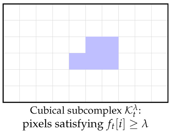
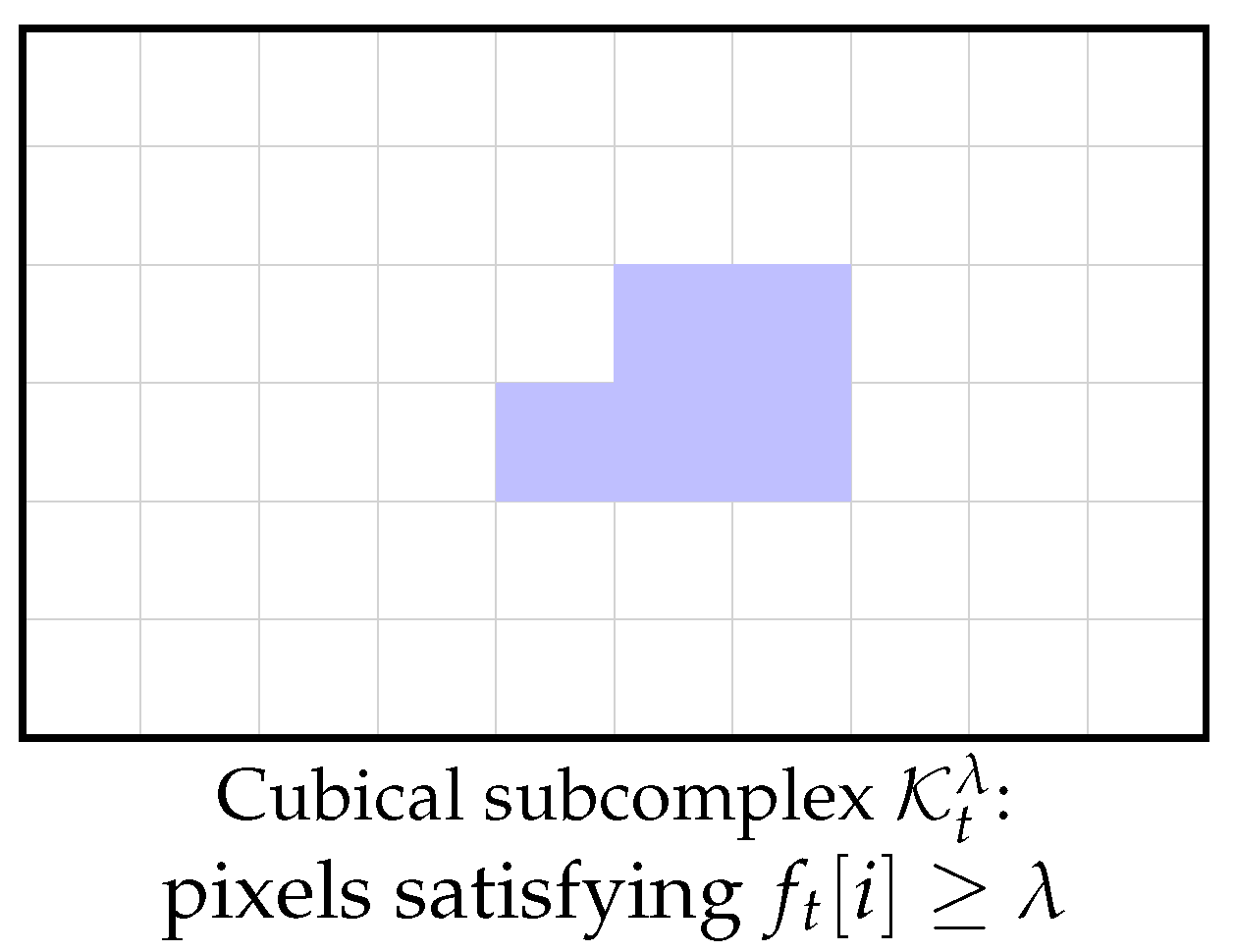
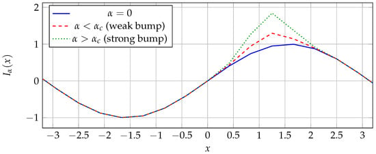
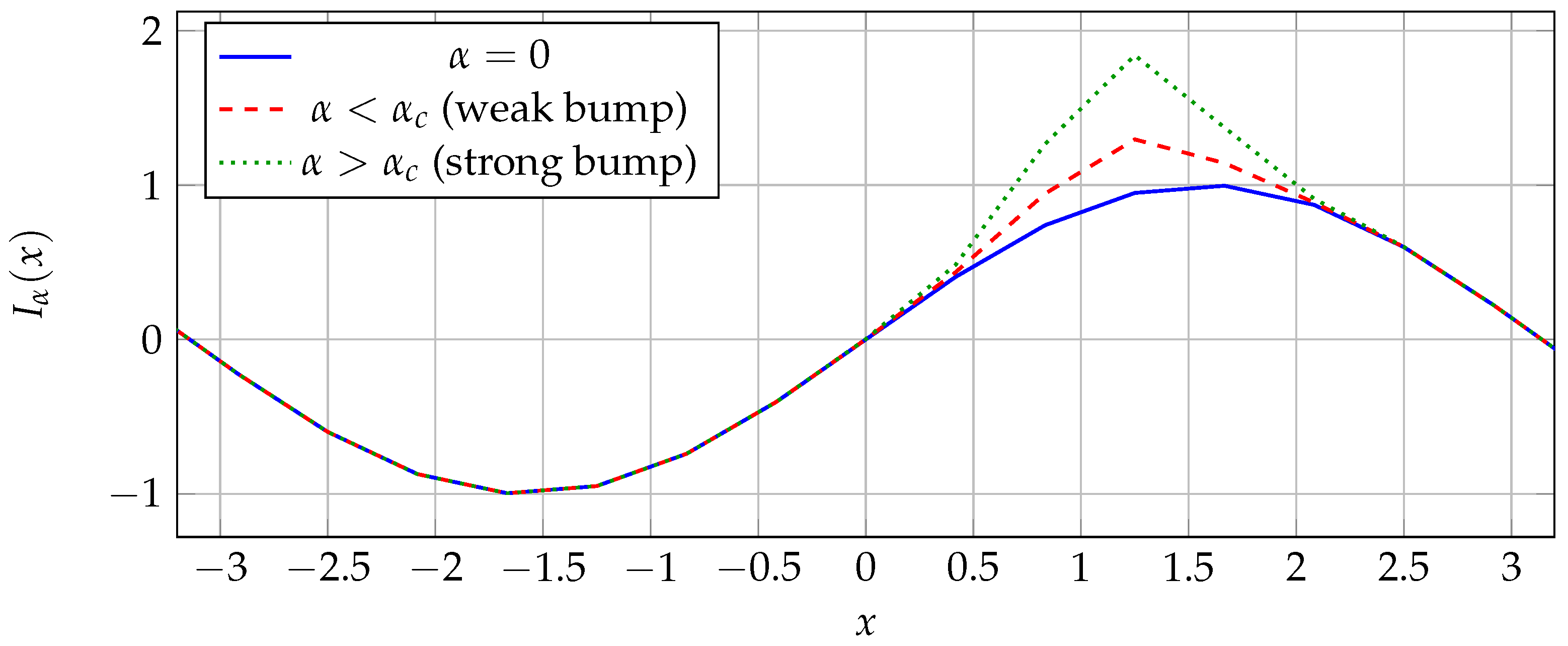
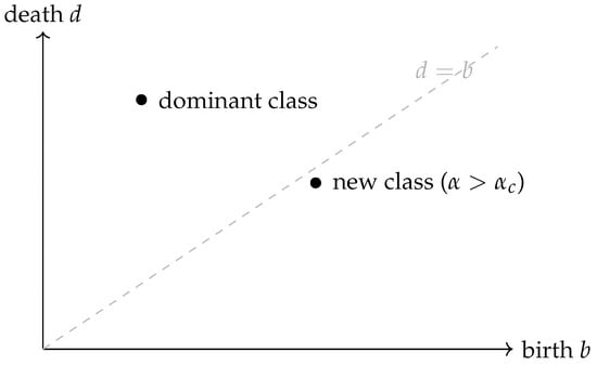
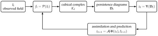


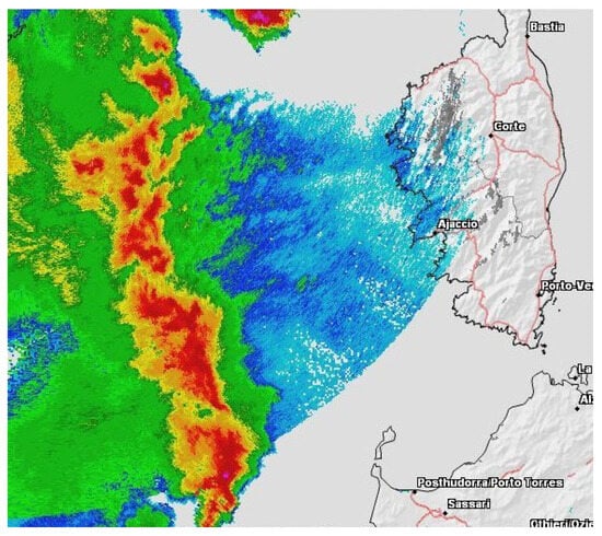
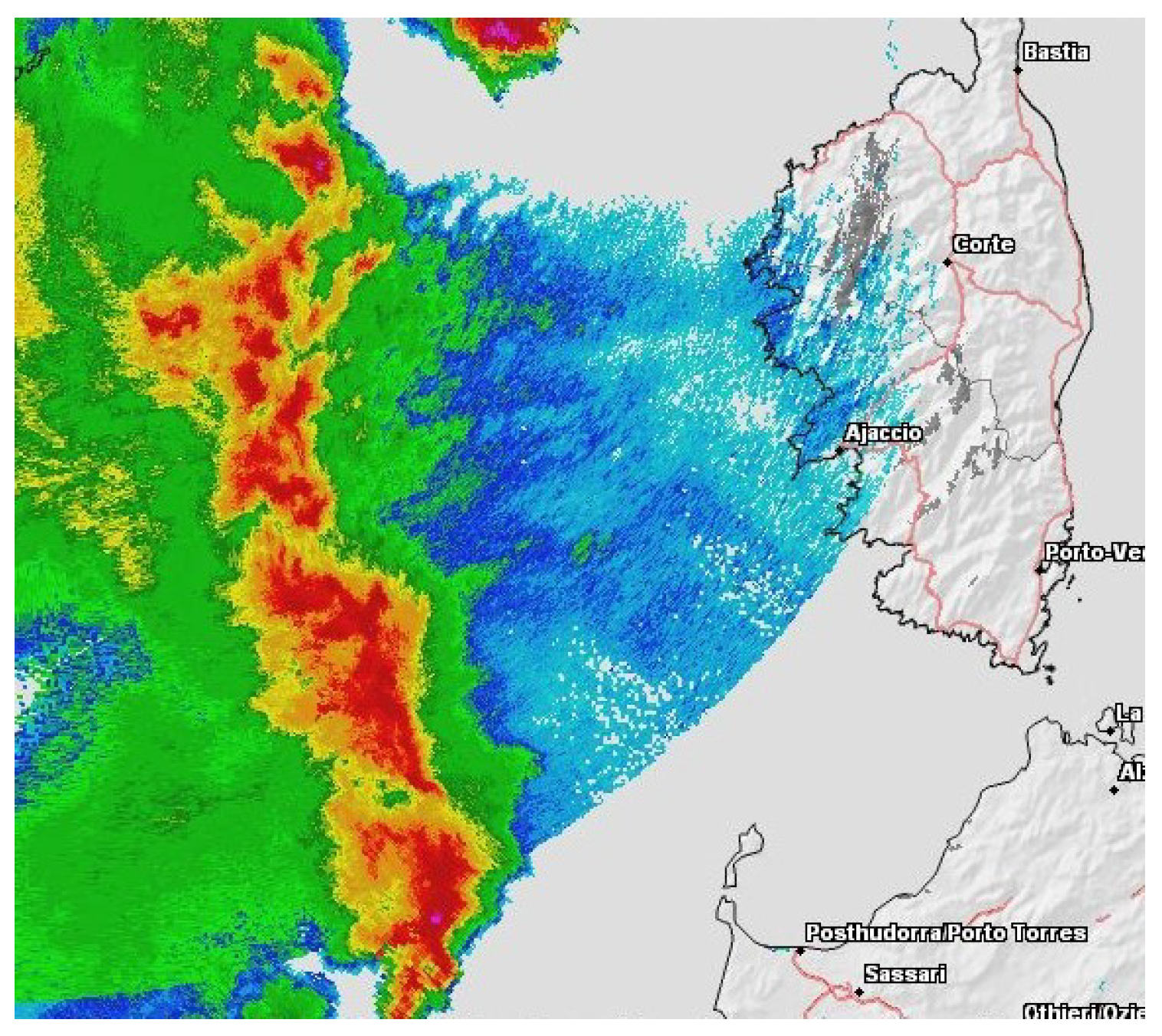
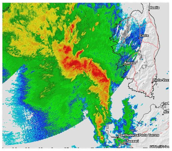
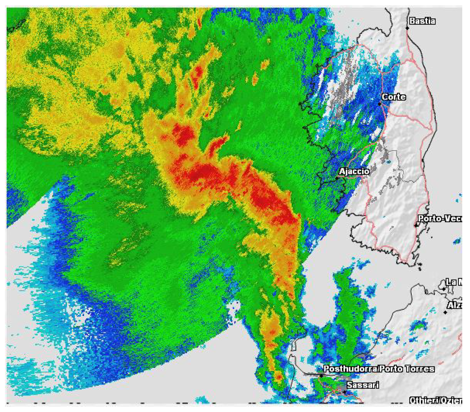
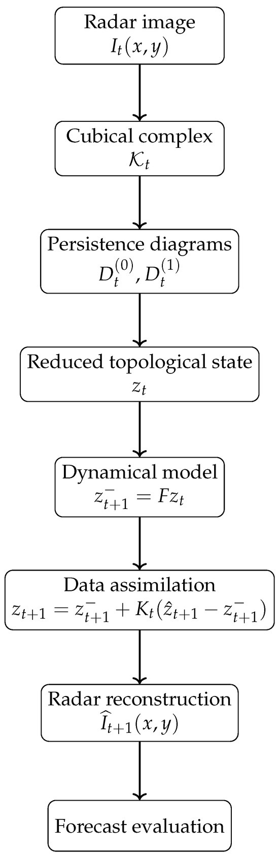
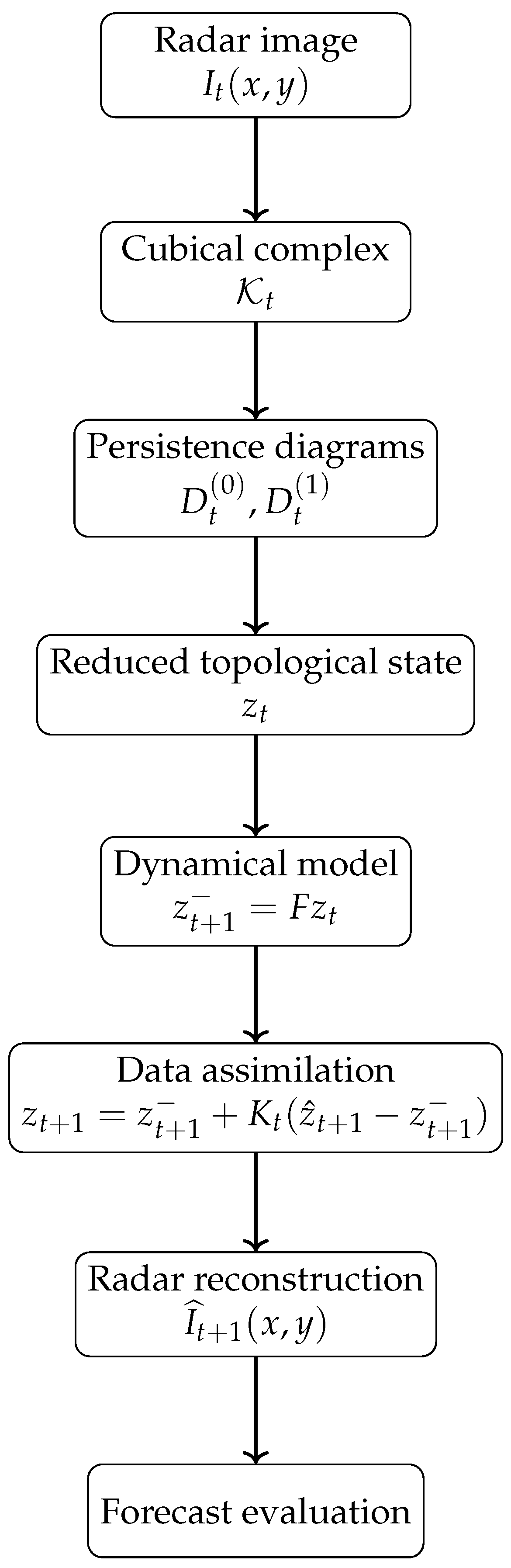
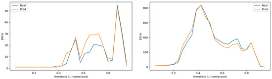
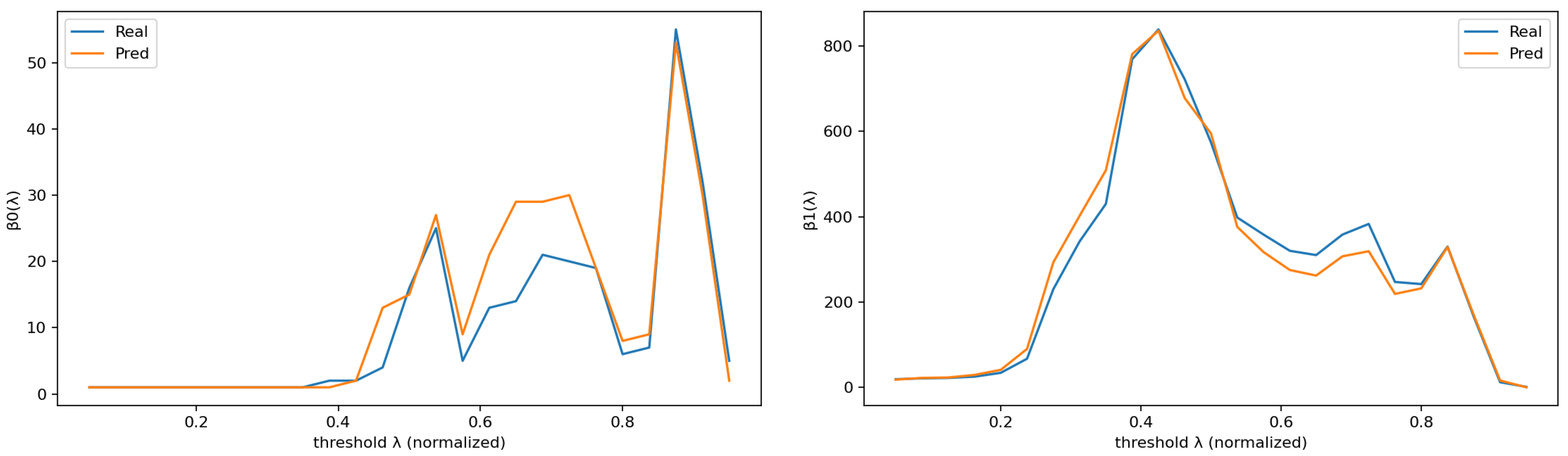
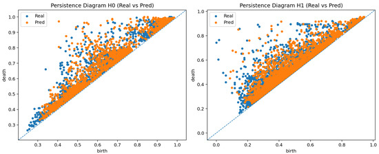
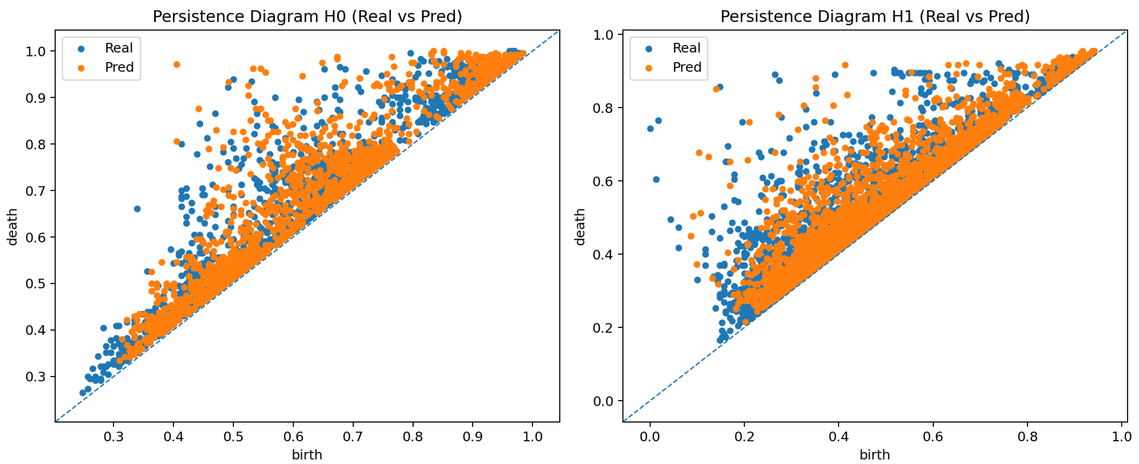
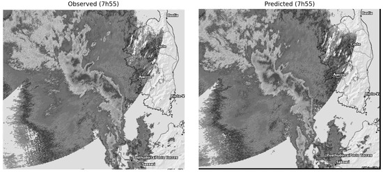
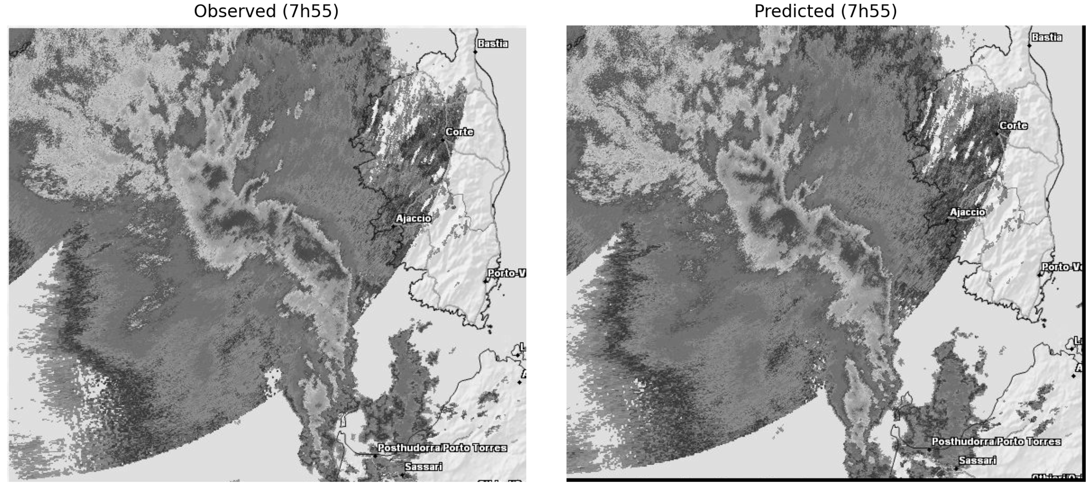
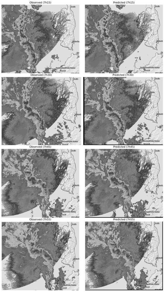
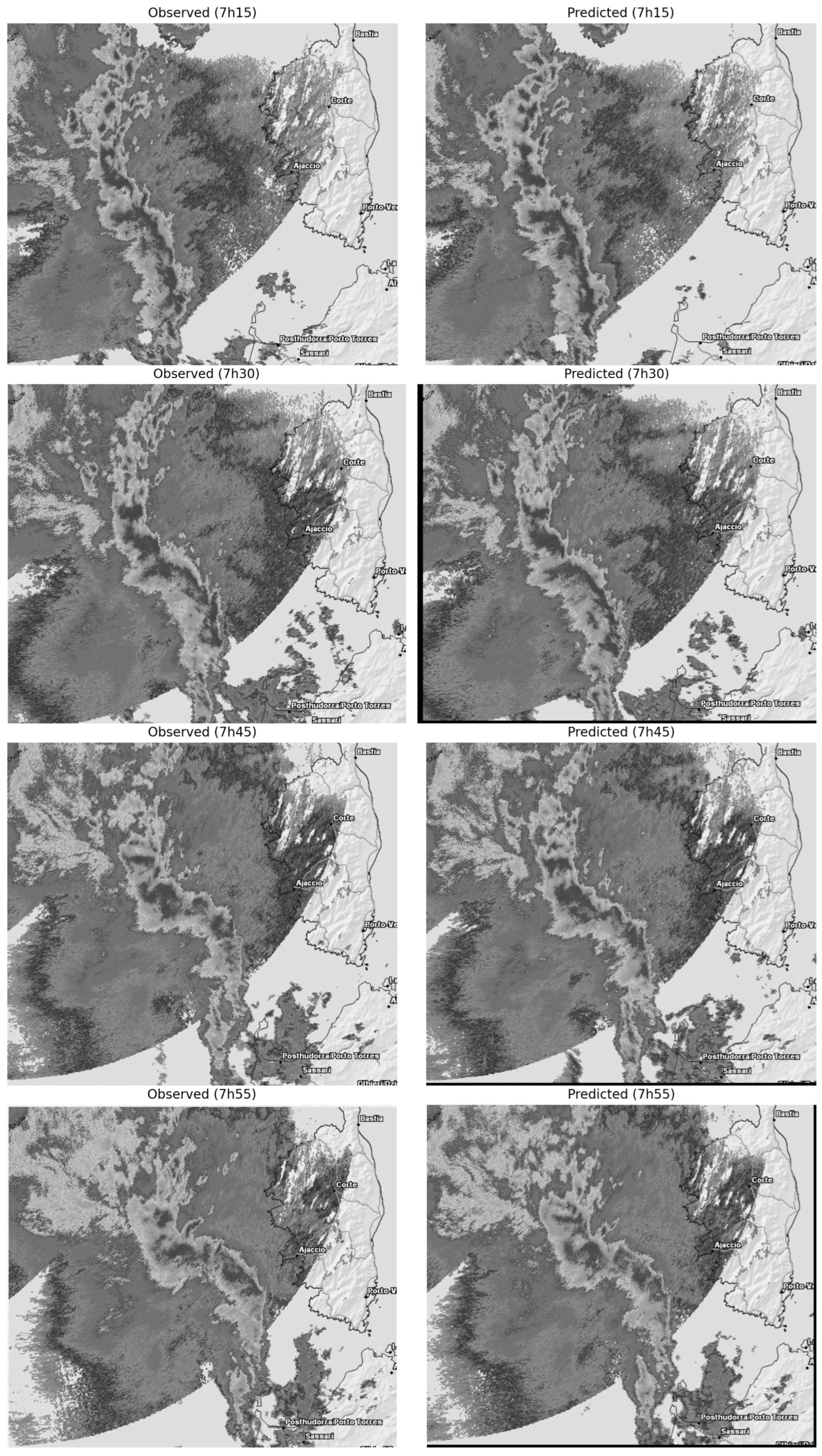
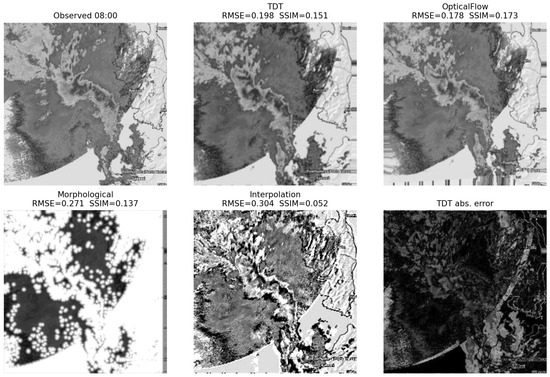
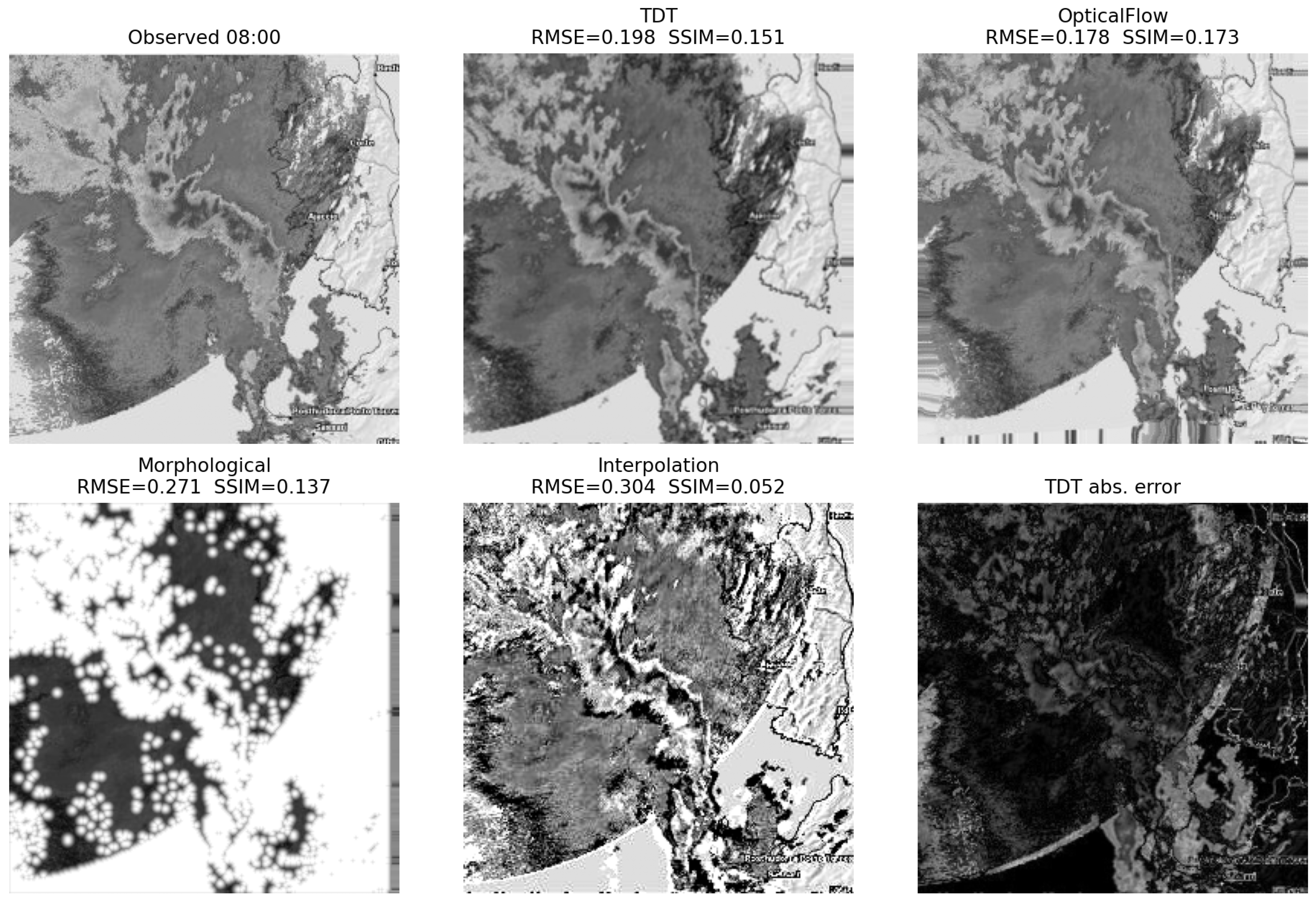
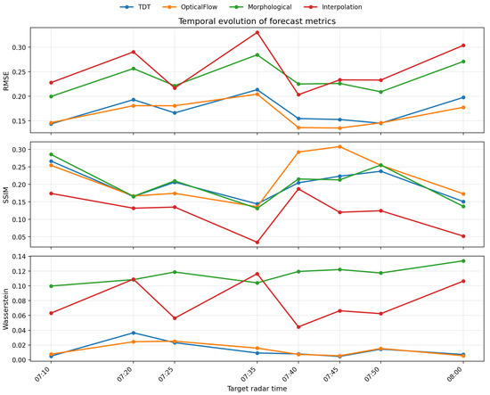
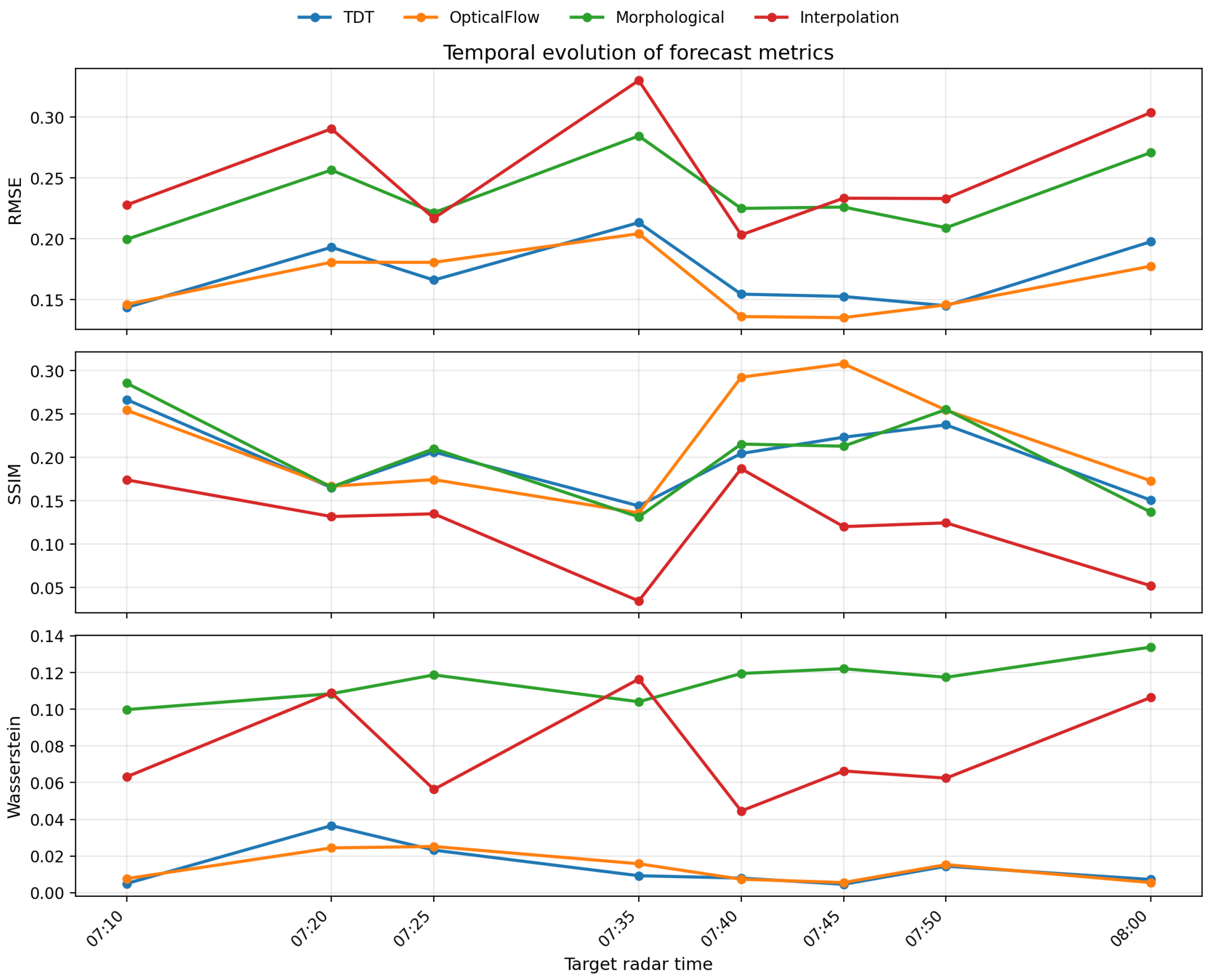
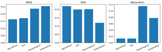
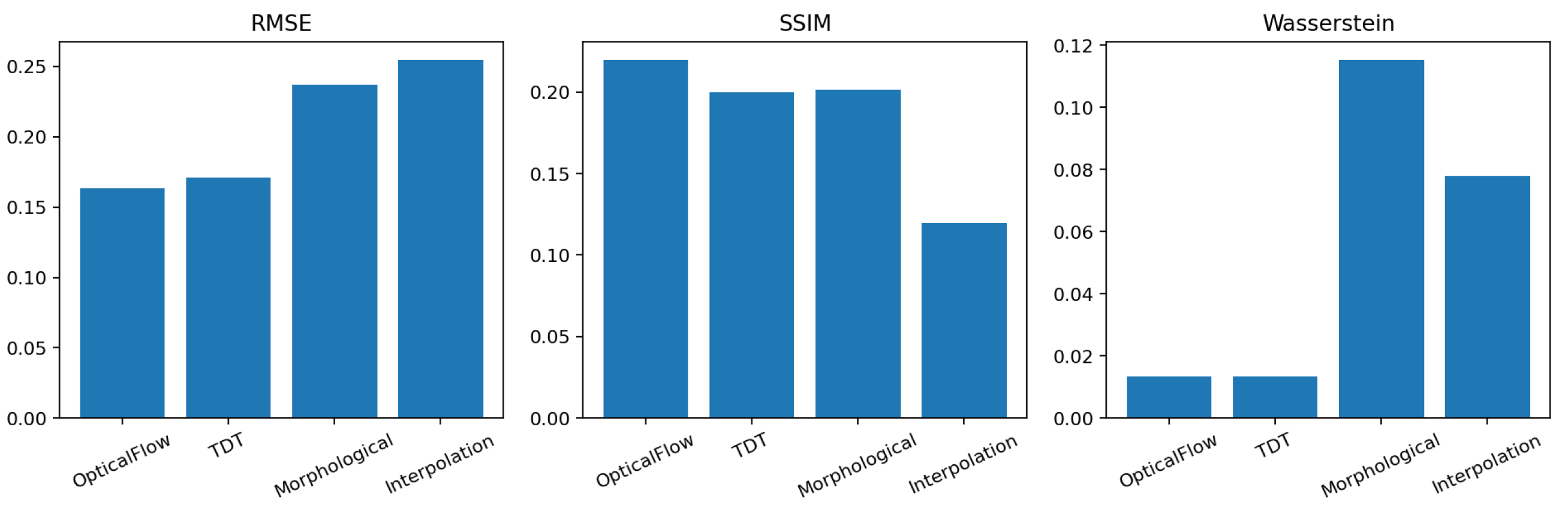

Disclaimer/Publisher’s Note: The statements, opinions and data contained in all publications are solely those of the individual author(s) and contributor(s) and not of MDPI and/or the editor(s). MDPI and/or the editor(s) disclaim responsibility for any injury to people or property resulting from any ideas, methods, instructions or products referred to in the content. |
© 2026 by the authors. Licensee MDPI, Basel, Switzerland. This article is an open access article distributed under the terms and conditions of the Creative Commons Attribution (CC BY) license.