


Abstract
This paper examines whether a residual structural state extracted from cross-asset downside-risk dependence contains incremental information for forecasting next-day market downside risk beyond a strong heterogeneous autoregressive (HAR) benchmark. The empirical analysis uses Binance intraday data from September 2019 to December 2025 and a fixed sample of 24 liquid cryptocurrencies obtained through explicit data-quality screening and sample diagnostics. The forecasting target is the log of an equal-weight cross-sectional downside-risk index constructed from strictly valid asset-level realized downside semivariance measures. The empirical design is deliberately conservative: the market sample is fixed ex ante, the target is evaluated against Bitcoin (BTC) and Ethereum (ETH) dominance diagnostics, and asset-level HAR-type models are estimated recursively to generate ex-ante one-step-ahead residuals, from which rolling residual-dependence matrices and structural signatures are constructed. The selected residual state contains four components: average residual correlation, Frobenius-type deformation, influence concentration, and influential-set turnover. The evidence supports three qualified conclusions. First, the full residual state attains the lowest average QLIKE loss relative to the HAR benchmark, although the corresponding Diebold–Mariano test under the primary QLIKE loss does not reject equal predictive accuracy at conventional levels. Complementary Clark–West evidence on the nested log-scale comparison supports incremental predictive content for the level-state and full-state augmentations. Second, the strongest forecasting evidence comes from the full state rather than from deformation-only specifications. Third, event-window diagnostics show that structural reorganization is most pronounced around stress-entry and extreme-risk episodes, supporting an onset-sensitive rather than a long-lead early-warning interpretation. Overall, the evidence supports a cautious and statistically qualified predictive conclusion: residual market structure may contain incremental information for short-horizon downside-risk forecasting in cryptocurrency markets, especially around stress onset, but the result should not be interpreted as a decisive primary-loss improvement or as evidence that deformation alone dominates a strong benchmark.
Keywords:
cryptocurrency volatility; downside risk; realized semivariance; HAR model; residual dependence; residual structural state; market downside-risk forecasting; stress-entry episodes; forecast evaluation MSC:
91G15
1. Introduction
Cryptocurrency markets are highly volatile, strongly interconnected, and prone to abrupt regime shifts, which makes short-horizon risk forecasting both economically relevant and empirically difficult. Recent surveys and forecasting studies show that this literature has become increasingly rich, but they also make clear that stable forecasting gains are difficult to obtain and often depend on the benchmark, the information set, and the regime under consideration [1,2,3,4]. At the same time, evidence of cross-cryptocurrency predictability and connectedness suggests that useful information may lie beyond single-series dynamics [5,6]. The relevant empirical question is therefore not whether one can generate many cross-asset summaries, but whether a disciplined structural design can provide qualified incremental predictive evidence beyond a strong benchmark.
Our starting point is the realized-volatility forecasting literature. The development of realized measures from intraday data provided a formal basis for measuring and forecasting daily volatility with greater informational content than lower-frequency proxies [7]. Within that literature, the heterogeneous autoregressive (HAR) model remains a natural empirical benchmark because it captures multi-horizon persistence in a parsimonious and empirically competitive way [8]. This benchmark remains central in cryptocurrency applications as well: recent studies continue to treat HAR-type specifications as difficult-to-beat baselines even when richer information sets, model averaging, machine learning, or sentiment variables are introduced [3,4,9]. For that reason, the present paper evaluates the main structural extension against HAR rather than against weak univariate alternatives, while also supplementing that benchmark-centered design with a focused nonlinear robustness check.
A second motivation concerns the target itself. Standard realized-variance measures treat positive and negative intraday returns symmetrically, whereas many practical risk questions are driven disproportionately by adverse moves. Realized semivariance therefore provides a natural basis for isolating downside variation and aligning the forecasting target more closely with market stress [10]. More recent work on realized downside and upside measures reinforces the point that asymmetric risk objects need not behave like aggregate volatility and may respond differently to asymmetric information sets [11]. This distinction is especially relevant in cryptocurrency markets, where crashes, liquidation cascades, and abrupt stress episodes are central empirical features.
The central idea of this paper is deliberately narrow. We do not ask whether broad classes of cross-asset methods are uniformly useful, nor do we claim that market topology alone delivers a superior forecasting system. Instead, we ask a more specific question: after controlling for strong own-series persistence through asset-level HAR-type residualization, does the residual cross-asset structure of downside risk contain incremental information for forecasting next-day market downside risk? This formulation matters because it shifts the empirical object away from raw co-movement and toward structural reorganization that remains after predictable asset-level persistence has been removed.
The empirical design is intended to limit data-mining concerns. We first construct a fixed sample of 24 liquid cryptocurrencies from Binance intraday data using explicit data-quality screening and sample diagnostics. We then build a market downside-risk target as the log of an equal-weight cross-sectional downside-risk index based only on strictly valid asset-day observations. Next, we estimate expanding-window HAR-type models for each asset and define residuals as ex-ante one-step-ahead forecast errors. Rolling residual dependence matrices are then mapped into a small set of structural summaries. To avoid feature inflation, the main residual state is restricted to four components only: average residual correlation, Frobenius-type deformation, influence concentration, and influential-set turnover.
The paper makes three contributions. First, it develops a conservative forecasting design for cryptocurrency market downside risk that combines a fixed sample, explicit data-quality screening, strict information timing, and parsimonious state construction. Second, it introduces a residual-state framework that separates predictable asset-level persistence from residual cross-asset structure before forecasting the market target. Third, it evaluates that state using out-of-sample score comparison, formal nested forecast-comparison tests, a focused nonlinear benchmark check, event-window diagnostics, falsification exercises, and regime-conditional analysis. These contributions are predictive rather than causal in scope.
The intended interpretation is deliberately restrained. The paper does not claim causal identification, and it does not seek to establish that any single structural component dominates simpler benchmark specifications in all samples and all regimes, or that the selected state universally dominates broader forecasting classes. Instead, the contribution lies in testing whether a small residual structural state contains short-horizon predictive information under a conservative empirical design.
Because the primary QLIKE-based Diebold–Mariano evidence is not statistically decisive, the paper interprets the forecasting evidence as qualified rather than conclusive. The empirical support comes from the combination of lower average QLIKE losses, significant Clark–West evidence in the nested log-scale comparison, and regime-conditional patterns, rather than from a uniformly significant primary-loss test.
The remainder of this paper is organized as follows. Section 2 reviews the relevant literature. Section 3 presents the data, sample construction, target design, and methodology. Section 4 reports the main forecasting contest together with formal forecast-comparison tests and an extended benchmark comparison. Section 5 presents the event-window diagnostics. Section 6 reports the falsification exercises and regime-conditional evidence. Section 7 discusses the interpretation of the results. Section 8 states the main limitations. Section 9 concludes.
2. Related Literature
2.1. Realized-Volatility Forecasting and the HAR Benchmark
A natural starting point for this paper is the large literature on realized-volatility measurement and forecasting. The realized-volatility framework of Andersen et al. [7] showed how intraday data can be used to construct informative daily volatility measures, and Corsi [8] proposed the HAR model as a parsimonious way to capture heterogeneous persistence across daily, weekly, and monthly horizons. The HAR model remains central because it is simple, interpretable, and empirically competitive, especially when the objective is conservative out-of-sample forecasting rather than in-sample fit alone.
That benchmark-centered perspective is especially important in empirical finance because volatility is latent and forecast comparisons depend on imperfect proxies and the chosen loss function [12]. In cryptocurrency applications, HAR-type models also remain serious competitors. For example, Qiu et al. [9] show that HAR-type specifications remain effective even when model uncertainty and measurement-error adjustments are incorporated, while more recent studies continue to evaluate advanced models relative to HAR-style baselines rather than dismissing them outright [3,4]. The present study follows that conservative logic while also supplementing the benchmark-centered design with a focused nonlinear robustness check.
2.2. Downside Risk and Realized Semivariance
A second strand of literature motivates the choice of target. Standard realized-variance measures aggregate positive and negative intraday returns symmetrically, whereas many financial applications care disproportionately about adverse moves. Realized semivariance provides a formal way to isolate variation associated with negative returns and thereby focus directly on downside risk [10]. This distinction is not merely semantic: changing the target changes the object being forecast.
This paper adopts a downside-oriented target because the empirical phenomenon of interest is market stress rather than generic volatility. That choice is aligned with more recent work showing that downside and upside realized-volatility objects can display different predictive behavior and may respond differently to asymmetric information sets [11]. In this sense, the paper belongs to the literature that treats downside variation as a substantively distinct forecasting object rather than as a minor refinement of aggregate realized variance.
2.3. Cross-Asset Dependence, Connectedness, and Structural-State Representations
A third literature concerns the measurement of cross-asset structure. Early correlation-network work emphasized that asset correlation matrices can reveal economically meaningful market architecture rather than serving only as inputs to portfolio optimization [13]. A later connectedness literature formalized the idea that multivariate dependence can be interpreted as an economically meaningful system of transmissions and exposures [14]. The broad lesson of that literature is that cross-sectional structure matters, but also that structural summaries must be embedded in disciplined empirical designs if they are to be used for prediction rather than description.
In cryptocurrency markets, this literature has expanded rapidly. Existing work documents dynamic connectedness and integration across crypto assets [5], realized-volatility connectedness across Bitcoin exchange markets [15], graph-based volatility and return connectedness [16], and dynamic return/volatility network behavior in multi-coin systems [17]. Very recent work also explores whether time-varying cryptocurrency network features can improve volatility prediction directly [18]. These studies make the present paper more demanding rather than less demanding: any claim of novelty must be stated narrowly and defended carefully.
The present paper is therefore not positioned as a generic network-forecasting contribution. It differs from much of the existing connectedness literature in four ways. First, the object of interest is a market downside-risk target rather than return volatility in a broad sense. Second, cross-asset structure is extracted only after asset-level HAR-type persistence has been partialled out. Third, the empirical design is built on a fixed and explicitly screened market sample rather than on a mechanically drifting asset set. Fourth, the main state is deliberately parsimonious rather than feature-rich.
2.4. Cryptocurrency Volatility Forecasting
The literature on cryptocurrency volatility forecasting is now broad, ranging from GARCH-type models and HAR-type realized-volatility specifications to machine learning, model averaging, alternative information sets, and hybrid forecasting systems [1]. Several studies underscore both the promise and the instability of this domain. Ftiti et al. [2] show that forecast performance can change materially across market conditions, while Feng et al. [3] and Brauneis and Sahiner [4] show that richer or nonlinear models can improve performance, but not in a way that makes benchmark discipline irrelevant.
Closer to the present paper, Qiu et al. [9] show that spillover information from other cryptocurrencies can improve short-horizon forecasting of Bitcoin realized volatility. That result is important for our setting because it supports the broader idea that cross-asset information can matter for crypto volatility prediction. However, that literature typically remains either Bitcoin-centered, spillover-centered, machine-learning-centered, or based on raw rather than residual cross-asset structure. The present paper instead asks whether a small residual structural state, constructed after filtering out own-series persistence, provides qualified incremental predictive evidence for a market-wide downside-risk object under a benchmark-centered design that is later complemented by a focused nonlinear robustness check.
2.5. Gap in the Literature and Contribution of This Paper
Against that background, the gap addressed by this paper is specific. Existing work gives strong reasons to use HAR benchmarks, to consider downside-oriented realized measures, and to study cross-asset dependence. Existing crypto papers also show that spillovers, connectedness, and dynamic network features may contain predictive information. What is less developed is a conservative design that combines these ingredients in the cryptocurrency setting while explicitly separating predictable asset-level persistence from residual market structure and then asking whether that residual structure provides qualified incremental predictive evidence for short-horizon downside-risk forecasting. Accordingly, this paper does not interpret lower average QLIKE losses as statistically decisive evidence on their own. The forecast evidence is treated as qualified and is read jointly with the QLIKE-based DM results, the nested Clark–West tests, and the regime-conditional diagnostics.
The contribution of this paper is therefore not that it introduces an entirely new forecasting architecture, nor that it proves topology or deformation to be universally dominant. The contribution is narrower and, in our view, more credible: once a fixed market sample is established, once the downside target is validated against concentration diagnostics, and once asset-level persistence is partialled out with expanding-window HAR-type models, a small residual structural state can be evaluated as a potential source of incremental next-day predictive information. At the same time, this paper is designed so that any positive evidence must be interpreted together with limiting evidence, including the possibility that deformation-only specifications remain weaker and that predictive strength is concentrated around stress periods rather than distributed uniformly across time. That combination of discipline and restraint defines the intended contribution of the study. In the revised empirical design, this evaluation is complemented by formal nested forecast-comparison tests and a focused nonlinear benchmark comparison, both intended to strengthen the empirical defense of the main result rather than to redefine this paper as a machine-learning horserace.
The literature therefore motivates three core elements of the present study: a strong HAR benchmark, a downside-oriented target, and a cross-asset structural representation. The remaining issue is how to combine these elements in a disciplined empirical design for cryptocurrency markets. This section describes the data, the sample-construction procedure, and the market downside-risk target, before presenting the residualization framework, the rolling dependence engine, the selected structural signatures, the forecasting protocol, the formal forecast-comparison tests, and the focused nonlinear benchmark check.
3. Data and Methodology
3.1. Data Source and Initial Candidate Sample
The empirical analysis is based on Binance intraday spot-market data covering the period from September 2019 to December 2025. The starting point is a pre-screened panel of 30 liquid USDT-quoted cryptocurrencies. Binance is used for pragmatic reasons: it provides broad cross-sectional coverage, relatively long continuous histories for major spot pairs, and high trading activity relative to most alternative centralized exchanges.
The forecasting exercise is conducted at a daily frequency, but the daily measures are constructed from intraday returns. In the extracted daily panel used for this paper, intraday support diagnostics are recorded on a 96-bin-per-day grid, corresponding to 15 min intervals within a UTC day. For that reason, the paper refers throughout to intraday support rather than using the narrower label “hourly.” This distinction matters because the validity of realized downside-risk measures depends not only on the existence of a daily observation but also on the quality and extent of the underlying intraday support.
The paper does not use the initial 30-asset panel mechanically. Instead, the final analysis sample is obtained through a sequence of explicit data-quality and temporal-stability filters designed to ensure that the retained universe is economically meaningful and statistically defensible. In highly volatile cryptocurrency markets, weak sample construction can contaminate every later stage of the analysis, especially when the object of interest is cross-asset structural reorganization rather than the dynamics of a single dominant coin.
3.2. Data-Quality Screening and Sample Diagnostics
The first layer of screening is applied at the asset level. For each candidate symbol, we compute summary diagnostics related to data availability and intraday support, including the share of days with available observations, the share of days satisfying strict return validity, the average number of supported intraday bins, average coverage, off-grid behavior, and average missing-bin counts. These diagnostics are used to construct a composite quality ranking and an initial classification of assets.
A second layer of screening is then applied to the time dimension. The motivation is that a symbol may look acceptable in unconditional averages while still exhibiting clusters of weak months or poor behavior around stress episodes. We therefore evaluate monthly quality profiles and stress-window behavior separately. A key issue in this step is that some weak months are common to the exchange-level panel rather than asset-specific. Treating those common months as symbol-level failures would unfairly penalize the entire universe. To avoid that problem, we distinguish Common Weak Months from idiosyncratic weak months. A month is treated as common-weak when panel deterioration is broad-based across the universe rather than concentrated in a small subset of symbols.
This adjustment matters for two reasons. First, it preserves a fixed and economically coherent analysis sample when temporary panel weakness is exchange-wide rather than asset-specific. Second, it prevents later structural results from being driven by mechanical composition shifts caused by unnecessarily excluding otherwise usable symbols. Detailed symbol-level diagnostics are reported in the Appendix B so that the main text can remain focused on the final analysis design.
3.3. Final Analysis Sample
After the summary diagnostics, temporal screening, and common-month adjustment, the final analysis sample is fixed to 24 cryptocurrencies: {ADA, ALGO, ANKR, ATOM, BAT, BNB, BTC, DASH, DOGE, ENJ, ETC, ETH, FET, IOTA, LINK, LTC, NEO, ONT, THETA, TRX, VET, XLM, XRP, ZEC}. Four additional assets (CHZ, XTZ, RVN, and HBAR) are retained only for robustness analysis, while two assets (STX and ARPA) are excluded from the main analysis sample. The empirical design is therefore built on a fixed rather than a time-varying market sample. This is a conservative choice: a fixed sample reduces the risk that later changes in dependence or market structure are simple artifacts of universe turnover rather than genuine market reorganization. Table 1 reports the final analysis-sample lock and retained tiers.
Table 1.
Final analysis-sample lock and retained tiers.
3.4. Intraday Returns and Daily Downside-Risk Measures
Let denote the intraday price of asset i on calendar day t and intraday bin b. Intraday log returns are defined as
Using these returns, we construct an intraday-based realized downside-risk measure for each asset-day:
where denotes the number of supported intraday bins on day t, and is the indicator function. This object is the downside analogue of realized-volatility measures constructed from intraday returns and is conceptually aligned with the realized semivariance literature [7,10,19,20].
An asset-day enters the main analysis only if it satisfies a strict validity filter. This requirement ensures that downside-risk measurement is based on adequately supported intraday returns and that weakly supported or silently repaired observations do not contaminate later cross-sectional structure.
3.5. Market Target Construction
The main forecasting target is a market-level downside-risk index constructed from the fixed 24-asset sample. Let U denote the main analysis sample. For each day t, define
where is the set of strictly valid asset-days on day t, and . We then define the positive-scale target
with a small fixed constant used only for numerical stability, and the forecasting variable
Two remarks are important. First, is an equal-weight cross-sectional downside-risk index; it is not exactly the same object as the intraday downside semivariance of an explicitly rebalanced equal-weight market portfolio. Second, a daily target observation is retained only if cross-sectional breadth is sufficiently high. In the empirical implementation, the breadth filter requires at least of the fixed sample to be valid on that day:
This definition is chosen for transparency and robustness. It preserves the downside-risk interpretation, remains tied to a fixed market sample, and avoids constructing the market target from a single dominant anchor. Economically, the equal-weight construction is used as a market-measurement choice rather than as a claim about a directly investable portfolio. It is intended to capture broad cross-sectional downside stress and to reduce mechanical dominance by the largest coins.
Because the forecasting variables are log-transformed downside-risk series, stationarity diagnostics can be useful for documenting their time-series properties. However, the empirical design is based on recursive out-of-sample forecast evaluation rather than on a static long-run equilibrium specification. The manuscript therefore does not use augmented Dickey–Fuller or other unit-root pretesting as a sample-selection or model-selection filter. Forecast comparisons are interpreted through their out-of-sample loss performance, with stationarity considerations treated as descriptive diagnostics rather than as identifying assumptions of the forecasting design.
3.6. Dominance Diagnostics
A necessary concern in cryptocurrency panels is that any market-level target may in fact be a disguised proxy for BTC or ETH. To address that concern, the target-construction stage includes explicit dominance diagnostics. We compare the main market target against BTC-only downside risk, ETH-only downside risk, and a leave-BTC/ETH-out version of the cross-sectional downside index. We also track date-level contribution shares of BTC and ETH within the aggregate downside measure.
These diagnostics serve a narrow but important role. They do not prove economic independence from large-cap anchors, but they do test whether the market target collapses once BTC and ETH are removed. In the empirical design used here, the target remains highly stable under that leave-out exercise, which supports the interpretation of the target as a market-wide downside-risk object rather than a simple large-coin proxy.
Figure 1 visualizes the retained market downside-risk target and shows that the constructed index captures several sharp downside-risk episodes over the sample.
Figure 1.
Main market downside-risk target on eligible days. The series is the log of the equal-weight cross-sectional downside-risk index. The dashed horizontal lines are auxiliary visual reference lines included to facilitate reading of the series. Spikes correspond to periods of elevated market downside risk and provide a visual check that the constructed target captures episodic stress rather than only smooth background volatility.
Table 2 reports the dominance diagnostics for the market downside-risk target.
Table 2.
Dominance diagnostics for the market downside-risk target.
These diagnostics provide a scale-aware check without redefining the forecasting target. The leave-BTC/ETH-out correlation tests whether the target remains stable after removing the two largest anchors, while BTC and ETH contribution shares assess whether the positive-scale index is mechanically dominated by those assets. A fully asset-normalized aggregation would be a useful additional robustness extension, but it is not used as the main target because this paper intentionally forecasts the observed equal-weight downside-risk index.
3.7. Implementation and Reproducibility
The empirical analysis was implemented in Python 3.12.12 using the Kaggle Notebook environment. Data manipulation and panel construction used pandas and numpy; recursive estimation and numerical procedures used statsmodels and scipy; figure construction used matplotlib; and parquet input/output used pyarrow. A compact extract of the daily panel is also reported in Appendix (Table A2) to illustrate the data structure across assets and time.
Taken together, the data construction stage yields a fixed and quality-controlled market sample, an auditable downside-risk target, and explicit dominance diagnostics against major anchor assets. These design choices define the empirical objects of interest but do not yet determine how structural information is extracted. The next subsection presents the methodological design used to construct, evaluate, and interpret the residual structural state.
3.8. Overview of the Empirical Design
The empirical design is built around a simple principle: structural information should be extracted only after strong univariate persistence has been controlled for. For this reason, the analysis proceeds in four steps. First, asset-level downside-risk series are residualized with expanding-window HAR-type models. Second, rolling residual dependence matrices are estimated from those ex-ante residuals. Third, a parsimonious residual structural state is extracted from the rolling matrices. Fourth, that state is evaluated in a benchmark-centered out-of-sample forecasting design, which is later complemented by formal forecast-comparison tests and a focused nonlinear robustness check.
This ordering is central to the contribution of this paper. The objective is not to show that raw dependence is descriptively rich in a generic sense. The objective is to test whether residual market structure contains predictive information beyond what is already captured by strong univariate persistence. Figure 2 provides a schematic overview of the empirical design.
Figure 2.
Schematic overview of the empirical design. The workflow proceeds from data screening and fixed-sample construction to target design, residualization, rolling residual dependence estimation, structural-state extraction, the main forecasting contest on fixed common support, formal forecast-comparison tests, a focused nonlinear benchmark comparison, and the supporting event-window, falsification, regime-conditional, and ablation analyses.
3.9. Asset-Level Residualization
For each asset i, define
where is the strictly valid asset-level downside-risk proxy defined in Section 3.4. We then estimate a HAR-type model separately for each asset using only information available up to time :
where
In this asset-level residualization equation, the dependent variable is the current log downside-risk measure . The regressors are the previous-day value , the trailing seven-day average , and the trailing thirty-day average . All lagged averages are computed using only observations available before the residual date, which preserves the ex-ante timing of the residuals.
The model is estimated recursively in an expanding-window fashion. For each asset-day in the forecasting sample, we obtain an ex-ante one-step-ahead fitted value
and define the residual as
This residualization step is not intended to whiten the panel completely. Instead, it is intended to remove predictable own-series persistence while preserving any cross-sectional structure that remains after univariate dynamics have been partialled out. That surviving structure is the object of interest.
3.10. Rolling Residual Dependence Matrices
Let denote the cross-section of residuals on day t, where is the number of assets available in a valid window ending at t. Using a rolling window of length days, we estimate residual dependence by the sample correlation matrix of the residual panel within the window. Rather than imposing a parametric dynamic-correlation system such as DCC, the paper adopts this rolling nonparametric design for transparency and direct interpretability [21]. To improve numerical stability, the raw correlation matrix is regularized through simple identity shrinkage:
where is the sample residual correlation matrix at window end t, I is the identity matrix, and in the baseline design [22].
A rolling window is declared valid only if panel support inside that window is sufficiently broad. In the baseline implementation, the window must contain at least 45 complete daily rows and at least 20 available assets. This validity discipline matters because deformation-like signatures can otherwise be contaminated by moving support rather than by genuine structural change.
3.11. Structural-State Extraction
The rolling residual dependence matrices are mapped into a small number of structural summaries. We deliberately restrict attention to a parsimonious state representation in order to avoid feature inflation. The initial candidate set includes both level and deformation summaries; after a redundancy audit, the main paper retains four signatures only.
- Level integration.
The first signature is the average off-diagonal residual correlation:
where denotes the element of . This variable captures the overall degree of market integration in residual space.
- Deformation magnitude.
The second signature measures day-to-day structural change in the residual dependence matrix:
where is the Frobenius norm.
- Influence concentration.
To capture the concentration of structural importance across assets, we first define absolute node strength:
Let
The concentration signature is then the Herfindahl–Hirschman-type index
High values indicate that residual dependence is concentrated in a relatively small set of influential assets.
- Influential-set turnover.
Let denote the set of the top-K assets ranked by absolute node strength in window t. In the baseline implementation, . The influential-set turnover signature is
This variable captures instability in the composition of the most influential residual nodes.
- Redundancy control and state definition.
The larger candidate set also included first principal-component share, a fragmentation-style index, and spectral-shift measures. However, these variables were found to be highly redundant with the selected signatures. The main paper therefore retains only the four-signature state
To avoid look-ahead bias, each signature is standardized recursively. Let denote component k of the state vector. The standardized regressor is defined as
where and are computed using only information available up to forecast origin t. This anti-leakage discipline matters because otherwise the state variables would be scaled with future information.
3.12. Benchmark and State-Augmented Forecasting Models
The main forecasting task is one-step-ahead prediction of the log market downside target . The baseline benchmark is a HAR-type model estimated recursively:
where
Thus, in the market-level forecasting regression, the dependent variable is the next-day log downside-risk target, . The HAR information set at forecast origin t contains the current daily value , the trailing seven-day average , and the trailing thirty-day average . All lagged averages are computed using only observations available at or before the forecast origin.
To evaluate the selected structural state, we estimate the following models recursively.
- HAR benchmark.
- HAR + level-only state.
- HAR + deformation-only state.
- HAR + full selected state.
These models define the core linear forecasting contest. The main benchmark-centered comparison is between M1, M2, M3, and M4. Section 4 later supplements this core comparison with formal forecast-comparison tests and a focused nonlinear benchmark check.
3.13. Out-of-Sample Protocol and Loss Functions
All forecasting models are estimated in a strict expanding-window manner. No future information is used in residualization, state construction, standardization, or forecast generation. The baseline minimum training length is 365 daily observations, after which one-step-ahead forecasts are generated recursively across the remaining sample.
To ensure comparability across models, the main forecasting contest is evaluated on fixed common support. In practice, this means that the headline comparison is restricted to dates for which the target, the benchmark regressors, and the relevant state variables are jointly available after the recursive training burn-in has been imposed. This restriction prevents measured forecast gains from being driven by shifting support rather than by genuine differences in predictive content. For transparency, the Appendix (Table A3) also reports the broader HAR backbone support before common-support alignment. Because this common-support restriction reduces the number of evaluated forecasts relative to the broader HAR backbone, Table A1 in Appendix A reports attrition diagnostics comparing retained and excluded dates. These diagnostics are included to assess whether the common-support filter disproportionately removes systematically different market conditions, such as unusually high downside-risk days.
The primary loss function is the quasi-likelihood loss evaluated on the positive downside-risk scale rather than on the log scale:
This choice follows the broader volatility-forecast evaluation literature, which emphasizes that forecast comparison depends on the proxy used and on the properties of the loss function [12,23]. Because the forecasting regressions are estimated on the log target , the level forecast is obtained in implementation by the simple exponential back-transformation
The resulting QLIKE values are interpreted comparatively across models rather than as statements about exact unbiased level recovery.
As a secondary criterion, we report mean squared error on the log scale:
This paper focuses on the one-step-ahead horizon. This restriction is deliberate. Given the event-conditional nature of the structural signal, spreading attention across many horizons would increase complexity without necessarily clarifying the main phenomenon.
3.14. Formal Forecast-Comparison Test Design
To complement the score comparison, the paper also reports formal out-of-sample forecast-comparison tests relative to the HAR benchmark. Because is the primary loss function of this paper, Diebold–Mariano (DM) tests are computed from daily loss differentials of the form
Negative mean differentials therefore favor the alternative model.
Because the state-augmented specifications are nested extensions of the HAR benchmark, the paper also reports Clark–West (CW) tests based on log-scale squared forecast errors. The CW layer is included because a standard loss-differential comparison can be conservative in nested settings. All formal tests are computed on the same fixed common-support sample used in the headline forecasting contest.
3.15. Focused Nonlinear Benchmark Comparison
As a focused nonlinear robustness check, the paper also includes two recursive random-forest benchmarks estimated under the same no-leakage and fixed common-support design as the HAR-based models. The first benchmark, RF-HAR, uses only the HAR backbone regressors
The second benchmark, RF-HAR + state, augments the same backbone with the four selected state variables
The random-forest comparison does not use a random train-test split. It follows the same chronological expanding-window out-of-sample design as the HAR-based specifications. At each forecast origin, the training set contains only observations available up to that date, and the next-day observation is used as the test point. The reported test performance is therefore obtained from the sequence of recursive one-step-ahead forecasts on the fixed common-support evaluation dates.
3.16. Event-Window Diagnostic Design
To distinguish between pre-stress buildup, onset-sensitive reorganization, and post-shock adjustment, we complement the forecasting contest with an event-window analysis. Two types of events are considered. The first are stress-entry dates, defined as the first day on which the market target enters the high-risk regime after previously lying below it. The second are extreme-risk dates, defined by an upper-tail threshold of the target distribution. In the main implementation, stress-entry events are organized around the upper-decile threshold, while extreme-risk events correspond to the upper tail.
Around each event, we construct symmetric 11-day windows from to and study the average behavior of both level and deformation composites. The event-window summaries reported in the main text are based on retained common-support dates with fully observed symmetric windows. This step does not establish causality. Its role is descriptive and diagnostic: it shows whether the selected structural state tends to move mainly before stress, at stress onset, or after large downside realizations have already materialized [24].
3.17. Falsification and Ablation
To reduce the risk that apparent forecasting gains are driven by chance alignment or overly flexible state design, the paper includes three basic falsification layers.
First, in a label-permutation placebo, the structural-state series are randomly reassigned across dates while the target and benchmark backbone remain fixed. Second, in a block-time permutation placebo, contiguous blocks of state observations are shuffled in time, preserving some local smoothness while breaking the original alignment. Third, in a raw-versus-residual comparison, the selected state is reconstructed from raw downside-risk dependence rather than from residual dependence. If the residual-state gain is genuine, it should dominate simple permutations and outperform the raw-state analogue in strength or reliability.
This paper also reports ablation exercises based on the full state. Each signature is removed one at a time from the full model to assess its incremental role in the observed lower average forecast loss. This ablation layer is especially important because the full-state model attains lower average QLIKE loss than the HAR benchmark even though deformation-only models are weaker on their own.
3.18. Interpretive Scope
The methodology is designed to support a predictive rather than causal interpretation. The paper does not claim that structural reorganization causes market stress in a structural-identification sense. Nor does it claim that deformation alone provides a general early-warning system. The appropriate interpretation is narrower: after strong univariate persistence is removed, a parsimonious residual structural state contains incremental information for next-day downside-risk forecasting, especially around stress-entry and extreme-risk episodes.
The methodological design described above yields a parsimonious residual structural state, a benchmark-centered forecasting contest, formal forecast-comparison tests, and a focused nonlinear robustness check. The next section reports the main out-of-sample forecasting results.
4. Main Forecasting Results
4.1. Benchmark-First Comparison Design
The main forecasting contest evaluates whether the selected residual structural state lowers average one-step-ahead forecast loss relative to a strong HAR benchmark. This benchmark-first design is essential. Given the strong persistence of downside-risk dynamics, small improvements over a serious HAR specification are more informative than large improvements over weak baselines. The empirical objective is therefore deliberately narrow: not to construct a universally dominant forecasting architecture, but to test whether residual structural information adds incremental value beyond a parsimonious and difficult-to-beat benchmark.
The core forecasting models are M1 (HAR benchmark), M2 (HAR plus level-only state), M3 (HAR plus deformation-only state), and M4 (HAR plus the full state). The selected state contains four parsimonious signatures: average residual correlation, Frobenius-type deformation, influence concentration, and influential-set turnover. The out-of-sample exercise is conducted recursively with an expanding-window protocol and is evaluated primarily by QLIKE on the positive target scale, with log-scale MSE reported as a secondary criterion.
To ensure comparability across models, the headline forecast comparison is conducted on fixed common support. In practice, this means that the main contest is restricted to dates for which the target, the benchmark regressors, and the relevant state variables are jointly available after the recursive training burn-in has been imposed. This restriction prevents measured forecast gains from being driven by shifting support rather than by genuine differences in predictive content.
4.2. Full-Sample Forecasting Contest
Table 3 reports the main out-of-sample score table for the benchmark and the three state-augmented specifications.
Table 3.
Main out-of-sample forecasting contest on fixed common support.
Three results are central. First, the HAR benchmark remains difficult to beat. The full state, M4, attains the lowest average QLIKE loss among the main competing models. Relative to the HAR benchmark, the average QLIKE reduction is about . However, as shown in the formal tests below, this average-loss reduction is not statistically decisive under the QLIKE-based Diebold–Mariano test. We therefore interpret it as directionally favorable average-loss evidence rather than as standalone proof of superior predictive accuracy under the primary loss function. The headline forecasting contest is evaluated on a fixed common-support sample of 1126 one-step-ahead predictions. By construction, this sample is smaller than the broader HAR backbone reported in Appendix A Table A1, which contains 1555 predictions before common-support alignment. To assess whether this reduction changes the composition of evaluated dates, Appendix A Table A1 compares the broader HAR backbone, the retained common-support dates, and the dates excluded by common-support alignment using support shares and HAR score diagnostics.
Second, level-only structural information is directionally favorable in average loss terms. The M2 specification attains lower average QLIKE than the HAR benchmark, with an average QLIKE reduction of roughly . This suggests that average residual integration and influence concentration may contain useful short-horizon information, although this evidence is not statistically decisive under the QLIKE-based DM test.
Third, deformation-only evidence is weaker. The M3 specification is essentially flat relative to the HAR benchmark in the full sample and does not dominate the level-only alternative. This negative result is substantively important. It implies that the incremental forecasting value observed in M4 cannot be described honestly as a pure deformation-only success.
4.3. Formal Forecast-Comparison Tests
To complement the score comparison in Table 3, we report formal out-of-sample forecast-comparison tests relative to the HAR benchmark. Because QLIKE is this paper’s primary loss function, Diebold–Mariano (DM) tests are computed from daily QLIKE loss differentials. Because the state-augmented models are nested extensions of the HAR benchmark, we also report Clark–West (CW) tests based on log-scale squared forecast errors. All tests are conducted on the same fixed common-support sample of 1126 one-step-ahead forecasts used in the headline forecasting contest.
Table 4 reports the formal out-of-sample forecast-comparison tests relative to the HAR benchmark.
Table 4.
Formal out-of-sample forecast-comparison tests relative to the HAR benchmark.
The distinction between the two formal tests is important. The Diebold–Mariano test is aligned with this paper’s primary QLIKE loss and therefore provides the most direct inference for the primary evaluation criterion. Under this test, the lower average QLIKE loss of the full-state specification is not statistically decisive. The Clark–West test answers a related but different question: whether the nested state-augmented forecasting equations contain incremental predictive content under log-scale squared forecast errors. The significant Clark–West results are therefore interpreted as complementary nested-model evidence, not as a substitute for primary QLIKE-based significance.
The formal tests refine the interpretation of the full-sample gains. For both the level-state model (M2) and the full-state model (M4), the DM statistics are directionally consistent with lower average QLIKE, but they do not provide strong statistical evidence at conventional levels. By contrast, the CW tests support the incremental contribution of the level-state and full-state augmentations relative to the HAR benchmark. The deformation-only model (M3) receives no such support. Taken together, the formal evidence supports a qualified interpretation: the favorable evidence is concentrated in the level-state and full-state augmentations, while deformation alone receives no comparable support.
4.4. Extended Benchmark Comparison
As a focused nonlinear robustness check, we add recursive random-forest benchmarks estimated under the same no-leakage, expanding-window, and fixed common-support protocol as the HAR-based models. The first benchmark, RF-HAR, uses only the HAR backbone regressors. The second, RF-HAR + state, augments the same backbone with the four selected state variables. This comparison is not intended as a comprehensive machine-learning horserace; its purpose is to assess whether the main result appears to be specific to the linear HAR class.
The nonlinear benchmark comparison does not overturn the main empirical ranking. The state-augmented random forest attains lower average QLIKE than the RF-HAR benchmark, which suggests that the selected state remains informative beyond the linear HAR specification. At the same time, the HAR + full-state model (M4) remains the strongest overall specification in QLIKE. The evidence therefore does not suggest that the main result is merely an artifact of comparing state-augmented models only to a linear HAR benchmark.
Table 5 reports the extended benchmark comparison including the focused nonlinear random-forest benchmarks.
Table 5.
Extended benchmark comparison including focused nonlinear random-forest benchmarks.
4.5. What Drives the Gain?
The comparison between M2, M3, and M4 is especially informative for interpretation. If deformation were the dominant mechanism on its own, one would expect M3 to perform at least as well as M2, to improve directly on the HAR benchmark, and to receive comparable support in the formal forecast-comparison tests. That is not what the data show. Instead, M2 is materially stronger than M3 in the full sample, M4 improves on both, and only the level-state and full-state augmentations receive support in the nested formal tests. The focused nonlinear benchmark comparison also does not overturn this ranking. The natural interpretation is therefore that the predictive content of the selected state comes from a combination of structural level information and structural reorganization rather than from deformation alone in isolation.
This is a more qualified conclusion than a deformation-dominance claim, but it is also the more credible one. The full state appears to summarize a broader market condition in which integration, concentration, and deformation interact. The evidence does not support a simpler story in which deformation by itself is sufficient to outperform a strong benchmark.
4.6. Interpretive Summary
The main forecasting evidence should be read as qualified rather than decisive. Four points summarize the results. First, the full residual state attains the lowest average QLIKE loss, but the QLIKE-based Diebold–Mariano test does not reject equal predictive accuracy relative to HAR. Second, the level-state and full-state augmentations receive complementary support from Clark–West tests in the nested log-scale squared-error framework. Third, deformation-only specifications remain weak in the full-sample forecasting contest and therefore do not support a deformation-dominance claim. Fourth, the focused random-forest comparison suggests that the state is not useful only inside the linear HAR class, although this remains a limited nonlinear robustness check rather than a comprehensive machine-learning comparison. The safest interpretation is therefore not that residual structure uniformly improves forecasts, but that the selected residual state provides qualified and regime-dependent evidence of incremental predictive content beyond a strong HAR benchmark.
These results define the contribution of the forecasting analysis more precisely. The positive result lies in the combined residual structural state, not in an unrestricted claim that matrix deformation alone delivers a general forecasting improvement. In that sense, the main forecasting evidence is supportive but deliberately narrow.
The forecasting contest shows that the full state attains the lowest average QLIKE loss, but it does not by itself establish statistically decisive superiority under the primary QLIKE-based DM test. The next section therefore studies the timing of the structural signal around stress-entry and extreme-risk episodes.
5. Event-Window Diagnostics
5.1. Why Event-Window Diagnostics Matter
The main forecasting contest evaluates whether the selected residual state lowers average out-of-sample forecast loss relative to the HAR benchmark. A separate question is how that state behaves around stress episodes. A structural signal can be economically informative for different reasons: it may rise well before stress and behave like an early-warning indicator; it may reorganize most sharply at stress onset; or it may respond mainly after large downside realizations have already occurred. These cases imply different interpretations of any observed forecast gain. For that reason, this paper complements average forecast comparisons with event-window diagnostics.
The analysis focuses on two event definitions. The first is the set of stress-entry dates, defined as days on which the market downside target first enters the upper-tail stress regime after previously remaining below it. The second is the set of extreme-risk dates, defined by an upper-tail threshold of the target distribution. Around each event, we evaluate the average path of the selected state over a symmetric event window and summarize the evidence using level and deformation composites. The event-window summaries reported below are based on retained common-support dates with fully observed symmetric windows.
The event-window analysis is descriptive and diagnostic. It is not a formal decomposition of the forecast-loss differences reported in Section 4. Its purpose is to examine when the selected state variables become active around stress episodes. Evidence on whether forecast performance differs across market conditions is reported separately in the regime-conditional loss analysis in Section 6.
5.2. Stress-Entry Profiles
The stress-entry evidence points to a clear empirical pattern: the selected residual structural state is most active at the onset of stress rather than far in advance of it. Figure 3 visualizes the average composite paths, while Table 6 summarizes the corresponding event-window diagnostics.
Figure 3.
Average event-window composite paths around retained stress-entry dates. The deformation composite rises modestly before the event but peaks at stress entry, supporting an onset-sensitive rather than a long-lead early-warning interpretation.
Table 6.
Event-window diagnostics for stress-entry and extreme-risk episodes.
The distinction between level and deformation components is important. The level composite moves only moderately around stress entry. By contrast, the deformation composite displays a sharp and localized onset spike. In the retained stress-entry sample, its average value is approximately in the pre-event window, rises to about at the event date, and falls to around afterward. This pattern is not consistent with a clean long-lead early-warning signal. It is more naturally interpreted as onset-sensitive reorganization.
Taken together, the stress-entry profiles suggest that the selected state is not simply tracking slow-moving background conditions. The main structural discontinuity occurs when the market is entering a high-risk configuration rather than well before that transition.
5.3. Extreme-Risk Profiles
The same qualitative conclusion emerges when the analysis is repeated for the extreme-risk subsample. Around upper-tail extreme-risk dates, the deformation composite again peaks most strongly at the event date itself. Pre-event values are positive, which indicates that some residual structural tension is already present before extreme downside realizations. However, that pre-event elevation remains materially smaller than the jump observed at the event date.
In the retained extreme-risk sample, the average deformation composite is about before the event, increases to roughly at the event date, and becomes slightly negative afterward, at approximately . This materially narrows the interpretation of the structural signal. If the selected state behaved as a pure early-warning device, the pre-event elevation would be expected to dominate the onset response. That is not what the data show. The dominant empirical regularity is instead that the strongest residual structural reorganization occurs when the downside-risk episode is beginning or actively materializing.
Figure 4 confirms that the extreme-risk evidence mirrors the stress-entry result in qualitative terms: pre-event tension is present, but the dominant structural reorganization remains concentrated at onset. This diagnostic pattern does not imply that deformation alone provides stable full-sample forecasting value. It instead suggests that deformation is episodic: it becomes visible around rare stress-onset dates, while its standalone contribution is diluted in the full evaluation sample.
Figure 4.
Average event-window composite paths around retained extreme-risk () dates. As in the stress-entry sample, the deformation composite is elevated before the event but reaches its largest value at the event date itself.
5.4. Implications for Interpretation
The event-window diagnostics therefore support a narrow but important conclusion. The selected residual state is best interpreted as an onset-sensitive descriptor of market reorganization, not as a clean deformation-only early-warning system. This interpretation also reconciles the event-window evidence with the weak full-sample performance of the deformation-only forecasting model. The event-window analysis describes the timing of structural activation around rare events, whereas the deformation-only forecast contest tests whether deformation alone delivers stable predictive gains across all common-support dates. The evidence supports the former statement but not the latter.
At the same time, the evidence is not purely post-shock either, because the deformation composite is already somewhat elevated before the event-window center. The most accurate characterization is therefore that residual structural tension builds modestly in advance, but its clearest and most reliable expression appears at stress onset.
This conclusion matters for the interpretation of the forecasting results in two ways. First, it is consistent with the regime-conditional evidence showing that the favorable forecast-score patterns are stronger around stress-entry and extreme-risk periods than in calm regimes. Second, it prevents overstatement. The contribution of this paper is not that structural deformation alone predicts crises far in advance. It is that a parsimonious residual structural state appears most informative when the market is reorganizing most sharply.
With that timing result in hand, the next section turns to falsification exercises and regime-conditional forecast evidence.
6. Falsification and Regime-Conditional Evidence
6.1. Why Additional Scrutiny Is Necessary
A modest full-sample forecasting gain is only meaningful if it cannot be reproduced easily by loose alignment, incidental timing, or overly flexible state construction. This issue is especially important in state-based forecasting exercises, where apparent improvements may arise from hidden data-mining, accidental synchronization, or support shifts across models. For that reason, this paper complements the main forecasting contest with three additional forms of scrutiny: permutation-based placebo tests, a raw-state versus residual-state comparison, and regime-conditional forecast decompositions. It then uses ablation evidence to assess which components of the state carry the signal inside the full model.
6.2. Permutation-Based Placebo Evidence
Table 7 reports the main falsification summary, and Figure 5 visualizes the distribution of placebo gains under label permutation.
Table 7.
Basic falsification evidence.
Figure 5.
Distribution of placebo gains under label permutation. The blue vertical line marks the realized full-state gain (the actual residual-state improvement relative to HAR). The realized full-state gain lies to the right of the placebo center, indicating that the observed improvement is stronger than what is typically produced by random realignment.
The placebo logic is straightforward. In the first exercise, the structural-state labels are randomly reassigned across dates while the target and HAR backbone remain fixed. In the second exercise, contiguous blocks of state observations are shuffled in time, preserving some local smoothness while breaking the original alignment between state and target. If the forecasting gain from the selected residual state is genuine, the realized improvement should exceed what is typically produced by these placebo realignments.
That is what the data show. The actual residual-state specification delivers a positive full-state gain relative to the HAR benchmark, whereas the median gain under label permutation is negative and the median gain under block permutation is also negative. Some placebo draws still generate small positive gains, so this is not an exhaustive falsification victory. It is, however, an important credibility check: the realized full-state gain is stronger than what emerges under simple random or blockwise realignment.
6.3. Raw-State Versus Residual-State Comparison
A second diagnostic asks whether the residual framing is doing genuine empirical work or merely relabeling raw dependence. To address this question, the selected structural state is reconstructed from raw downside-risk dependence rather than from residual dependence, and the forecasting comparison is repeated under the same benchmark design.
The raw-state analogue does not match the main result as strongly or as reliably as the residual-state specification. Its performance is materially weaker than that of the residual-state version, and the residual construction remains preferred under the support-aligned forecasting design. This distinction matters. It suggests that the useful signal is not simply generic market co-movement. Instead, the informative structure becomes sharper after predictable asset-level persistence has been removed, which is exactly the empirical object this paper set out to study.
6.4. Regime-Conditional Forecast Performance
The regime split sharpens the interpretation of the forecasting evidence. In the full sample, the full state attains the lowest average QLIKE among the four main competing models. That advantage becomes clearer in the stress-oriented subsets, including upper-decile stress days, upper-tail extreme-risk days, and stress-entry days. By contrast, the advantage of the full state weakens or disappears in the post-entry and calm subsets. This pattern is consistent with the event-window diagnostics in Section 5: the selected structural state is most informative when the market is entering or inhabiting a stressed configuration rather than after the transition has already passed.
At the same time, the regime decomposition does not rescue a deformation-only story. Even in stress-oriented subsets, the deformation-only specification remains weaker than the full state and does not establish a clean standalone advantage over the HAR benchmark. The evidence therefore points to deformation as an episodic and complementary component, not as an independent full-sample forecasting channel.
The regime-conditional loss analysis provides the forecast-performance counterpart to the descriptive event-window evidence. Unlike the event-window diagnostics, which only show when the state variables become active, Table 8 evaluates whether forecast scores differ across retained market-condition subsets.
Table 8.
Regime-conditional forecasting scores for the main competing models.
The regime decomposition clarifies the interpretation. The full state performs most favorably in stress-oriented subsets, including upper-decile stress days, upper-tail extreme-risk days, and stress-entry dates. By contrast, its advantage weakens or disappears in post-entry and calm subsets. This pattern supports a regime-dependent interpretation: the full-state signal is concentrated around stressful market configurations and is diluted in full-sample averages because such episodes are relatively rare.
6.5. Ablation Evidence
Table 9 reports the ablation evidence for the full-state model, and Figure 6 summarizes the corresponding performance losses visually.
Table 9.
Ablation results for the full-state model in the full sample.
Figure 6.
Ablation damage for the main signatures in the full-state model. Larger values indicate larger losses in forecast performance when the corresponding signature is removed.
The ablation exercise helps identify which components of the state carry the main forecasting signal inside M4. The results are informative, but they should not be overstated as a rigid universal ranking. In the full sample, removing Frobenius-type deformation produces the largest deterioration in forecast performance, while removing influence concentration also weakens the model materially. Removing influential-set turnover produces the smallest deterioration. By contrast, removing average residual correlation does not worsen full-sample QLIKE and in fact yields a slight improvement in the full sample. Its marginal role should therefore be interpreted more cautiously than that of deformation or concentration.
This pattern still helps reconcile the main empirical results. Deformation is clearly important inside the combined state even though deformation-only forecasting remains weaker on its own. At the same time, the evidence does not support an overly sharp claim that one single component dominates in all subsets and all regimes. The safer conclusion is that the full-state gain reflects the interaction of several state components, with deformation and concentration providing the clearest full-sample contribution, turnover contributing least, and average residual correlation showing less stable marginal evidence in the full sample.
6.6. What These Results Do and Do Not Establish
Taken together, the falsification, regime-conditional, and ablation results refine the contribution of this paper in four ways. First, they make it harder to dismiss the observed gain as a trivial timing artifact. Second, they show that residualization matters empirically, not just conceptually. Third, they clarify that the forecasting value of the state is concentrated around stress-entry and extreme-risk episodes rather than being regime-invariant. Fourth, they show that deformation is important as a component of the full state, but not as a clean standalone forecasting channel.
These results should still be interpreted cautiously. They do not provide causal identification, and they do not rule out every alternative explanation. In particular, the distance between the realized gain and the strongest placebo realizations is meaningful but not overwhelming. A more demanding evidence pack would include larger placebo suites, alternative block designs, and additional robustness layers. For that reason, the present falsification exercise should be read as a basic but useful credibility check rather than as an exhaustive identification strategy.
Taken together, the forecasting, event-window, regime-conditional, and falsification results support a narrower but more credible contribution than a generic topology-dominance claim. The remaining task is to interpret that contribution carefully, clarify its scope, and state the main limitations explicitly. These issues are addressed in Section 7.
7. Discussion
7.1. Main Empirical Message
The evidence in this paper supports a narrow and statistically qualified conclusion. After controlling for strong asset-level downside-risk persistence through expanding-window HAR-type residualization, the full selected residual state attains lower average QLIKE loss than the HAR benchmark, but the QLIKE-based Diebold–Mariano evidence is not statistically decisive. The complementary Clark–West tests provide stronger support in the nested log-scale squared-error framework, and the regime-conditional results indicate that the signal is concentrated around stress-entry and extreme-risk episodes. This combination of results supports cautious evidence of incremental predictive content, not an unrestricted claim of superior predictive accuracy under every evaluation criterion.
The revised evidence is stronger than a purely descriptive score comparison. In particular, the level-state model and the full-state model receive formal support in nested forecast-comparison tests relative to the HAR benchmark, whereas the deformation-only specification does not. At the same time, the QLIKE-based DM evidence remains directionally favorable but not decisive, which is consistent with the modest magnitude of the full-sample gains. This combination of results strengthens the main conclusion while also reinforcing the need for interpretive restraint.
At the same time, the results do not support a stronger claim that deformation alone dominates standard benchmarks or that structural summaries by themselves provide a clean early-warning system. Deformation-only specifications remain weaker than the full selected state and do not deliver a comparable full-sample result against the HAR benchmark. The strongest empirical result comes instead from the combined residual structural state, especially when the market is reorganizing into a stressed configuration.
This distinction is important. Structural language can easily outrun the actual forecasting evidence in this literature. The contribution of the present study is therefore not that it establishes a universal structural forecasting law. It is that it identifies a conservative and reproducible way to extract residual market structure and shows that this state contains useful short-horizon information, particularly around downside-risk transitions.
7.2. Why the Residual Framing Matters
One of the central design choices of this paper is to focus on residual rather than raw structure. This is not a cosmetic distinction. If raw cross-asset dependence alone were sufficient, then state variables constructed directly from raw downside-risk series should perform as strongly and as reliably as their residual-state counterparts. That is not what the data show. The raw-state analogue does not match the main result as strongly or as consistently as the residual-state design under the support-aligned forecasting comparison.
Conceptually, this matters because cryptocurrency markets are both highly persistent and highly integrated. In such an environment, raw dependence measures can be dominated by common persistence, broad market drift, or slow-moving conditions that are already partially absorbed by strong univariate benchmarks. Residualization changes the empirical object of interest. Rather than measuring total co-movement, it measures the structure of deviations from expected asset-level downside-risk dynamics. That residual structure is the object that appears to contain incremental forecasting content.
The focused nonlinear benchmark comparison reinforces this interpretation. The state-augmented random forest improves on the RF-HAR benchmark, which suggests that the selected state is not informative only within the linear HAR class. At the same time, the HAR + full-state specification remains the strongest overall model in QLIKE, so the nonlinear robustness check strengthens rather than overturns the main empirical ranking.
7.3. Why the Signal Is Strongest at Stress Onset
The event-window and regime-conditional results jointly indicate that the structural signal is most informative at stress onset rather than far in advance of it. This is an important empirical finding because it sharply narrows the interpretation of the state variables. The selected residual structural state should not be read as a long-lead crisis-warning system. Instead, it appears to summarize rapid market reorganization that becomes most visible when the market is entering a stressed downside regime.
That pattern is economically plausible. In highly reactive markets such as cryptocurrencies, structural reorganization may occur quickly, with cross-asset dependence intensifying, influence becoming more concentrated, and dependence structure adjusting abruptly as stress materializes. Under that interpretation, the state variables are useful not because they forecast distant future crises, but because they sharpen short-horizon forecasts precisely when market conditions are transitioning most abruptly.
7.4. What the Selected Signatures Appear to Capture
The ablation evidence helps clarify which parts of the selected state matter most inside the full specification, but it should not be read as implying a rigid universal ranking. In the full sample, Frobenius-type deformation and influence concentration show the clearest deterioration when removed, while influential-set turnover contributes least. The marginal role of average residual correlation is less stable in the full sample and should therefore be interpreted more cautiously than the other two core signatures.
This pattern still helps reconcile the broader empirical picture. Deformation is clearly important inside the combined state even though deformation-only forecasting remains weaker on its own and does not receive comparable support in the formal nested forecast-comparison tests. At the same time, the evidence does not support an overly sharp claim that one single component dominates in all subsets and all regimes. The safer conclusion is that the full-state gain reflects the interaction of several components, with the most robust full-sample contribution coming from deformation and concentration rather than from a single universally dominant channel.
7.5. Positioning the Contribution
The paper is best positioned as a contribution to short-horizon downside-risk forecasting under a disciplined residual-state design. Its value does not come from methodological extravagance. On the contrary, one of the strengths of the design is its restraint: a fixed sample, explicit data-quality screening, strict-valid target construction, ex-ante residualization, parsimonious state selection, strong benchmark comparison, formal nested forecast-comparison tests, a focused nonlinear robustness check, and basic falsification.
That positioning also implies a realistic reading of the contribution. The current evidence is stronger as a careful empirical paper in volatility forecasting and market-state measurement than as a claim of broad structural dominance. That narrower positioning is not a weakness; it is what makes the evidence credible.
The discussion above clarifies the main contribution of this paper and the most defensible interpretation of the empirical evidence. That interpretation, however, depends on several design choices and should be read together with this study’s limitations, which are stated explicitly in the next section.
8. Limitations
Several limitations should be acknowledged.
First, the market target is an equal-weight cross-sectional downside-risk index rather than the exact intraday downside semivariance of a continuously rebalanced market portfolio. This choice is deliberate and robust, but it narrows the interpretation of the target. The paper therefore speaks of market downside-risk forecasting in an index sense rather than claiming a fully portfolio-based target throughout.
Second, the empirical design is built on a fixed 24-asset sample selected from a larger pre-audited panel. This improves comparability and reduces composition-driven artifacts, but it also means that the results are conditional on a particular liquid-core representation of the market. A broader sample or a time-varying sample design could alter both the structural signatures and the magnitude of the forecasting gains.
Third, the fixed common-support design creates an additional form of sample attrition. This design is necessary for comparing all competing models on identical forecast dates, but it reduces the evaluation sample relative to the broader HAR backbone. For this reason, the Appendix(Table A1 in Appendix A) reports attrition diagnostics comparing retained and excluded dates. The headline results should therefore be interpreted as common-support forecast comparisons, not as claims about every date in the broader HAR-backbone sample.
Fourth, the forecasting value of the selected state is clearly regime-dependent. The full selected state attains its most favorable forecast-loss reductions in stress-entry and extreme-risk periods. This paper should therefore not be interpreted as establishing a universal improvement across all market conditions.
Fifth, the paper evaluates statistical forecast performance rather than direct economic utility. The results show modest improvements in forecast loss, but they do not by themselves establish portfolio value, trading profitability, or risk-management gains.
Sixth, a further limitation concerns the strength of statistical evidence under the primary loss function. Although the full-state model attains the lowest average QLIKE loss in the main forecast comparison, the QLIKE-based Diebold–Mariano test does not reject equal predictive accuracy relative to the HAR benchmark at conventional levels. The significant Clark–West results should therefore be interpreted as complementary nested-model evidence based on log-scale squared forecast errors, not as a substitute for primary QLIKE-based significance.
Seventh, although the revised manuscript adds formal forecast-comparison tests and a focused random-forest robustness check, it does not attempt a comprehensive comparison across broader machine-learning classes, alternative nonlinear learners, or extensive tuning regimes. The evidence should therefore be interpreted as showing incremental value beyond a strong HAR benchmark and a limited nonlinear check, rather than universal dominance over all forecasting approaches.
Eighth, the falsification exercises, while informative, remain basic. Label permutation, block permutation, and raw-versus-residual comparisons strengthen credibility, but they do not exhaust all placebo or identification concerns. More demanding placebo architectures, alternative block designs, and broader robustness suites would further strengthen the empirical defense.
Ninth, this paper is predictive rather than causal. The results do not identify structural transmission channels in a causal sense, nor do they establish that residual reorganization causes next-day downside risk. The appropriate interpretation is predictive and descriptive: the selected residual structural state contains incremental information about short-horizon market downside risk, especially when stress is emerging.
Finally, the analysis is conducted on Binance spot-market data. While Binance is an economically important venue, the results should not automatically be treated as exchange-invariant. Cross-exchange validation remains a useful direction for future work.
These limitations narrow the interpretive scope of this paper, but they do not overturn its central empirical message. They instead clarify the setting in which the contribution should be understood. The final section summarizes that contribution and outlines the main directions for future work.
9. Conclusions
This paper examined whether a residual structural state extracted from the cross-asset dependence of cryptocurrency downside risk improves short-horizon market downside-risk forecasting beyond a strong HAR benchmark. The empirical design was intentionally conservative. A fixed and quality-controlled liquid-core sample was established after explicit data-quality screening and temporal diagnostics; the market target was validated against BTC/ETH dominance diagnostics; asset-level HAR-type models were estimated recursively to construct ex-ante residuals; and a parsimonious structural state was extracted from rolling residual dependence matrices.
The main conclusion is cautious but positive. A selected residual structural state improves next-day downside-risk forecasting relative to the HAR benchmark. The gain is modest in full-sample averages, but it becomes stronger around stress-entry and extreme-risk episodes. This indicates that residual market structure contains useful information precisely when market conditions are reorganizing most sharply.
The revised evidence also strengthens the empirical defense of this conclusion. The level-state and full-state augmentations receive formal support in nested forecast-comparison tests relative to HAR, whereas the deformation-only specification does not. A focused nonlinear benchmark comparison further shows that state augmentation improves on the RF-HAR benchmark without overturning the main empirical ranking. At the same time, the DM evidence based on QLIKE remains directionally supportive rather than decisive, which is consistent with the modest magnitude of the full-sample gains.
At the same time, the results do not support an unrestricted deformation-only or early-warning interpretation. Deformation-only specifications remain weaker than the combined state and do not deliver a comparable full-sample result against the HAR benchmark. The strongest evidence comes from the combined residual state rather than from any single structural channel considered in isolation. Basic falsification exercises further show that the observed gain is stronger than simple permutation-based placebo gains, while raw-state constructions do not reproduce the residual-state result as strongly or as reliably.
Taken together, the evidence supports the following interpretation. In cryptocurrency markets, the most useful structural information is neither generic raw co-movement nor a standalone deformation-only signal. It is a residual, parsimonious, and event-conditional market state that becomes especially informative when downside-risk stress is beginning to materialize. This is a narrower conclusion than a broad structural-dominance claim, but it is also a more defensible one.
Future work can extend the analysis in several directions, including richer falsification architectures, alternative dependence estimators, cross-exchange validation, broader sample designs, direct economic-value evaluation, more extensive nonlinear benchmark comparisons, and more explicit links to portfolio and risk-management applications. In its current form, the paper provides qualified evidence that a disciplined residual-state design can add incremental information to benchmark-based downside-risk forecasting in cryptocurrency markets. The evidence is strongest when lower average QLIKE losses are read together with nested Clark–West tests and stress-oriented regime decompositions. However, because the primary QLIKE-based Diebold–Mariano test is not statistically decisive, the conclusion should remain cautious: the selected residual state appears informative in a qualified and regime-dependent sense, rather than uniformly superior under all forecast-comparison criteria.
Author Contributions
R.-H.L.: methodology, software, validation, formal analysis, investigation, data curation, writing—original draft preparation, visualization. S.-C.C.: validation, formal analysis, investigation, writing—review and editing. J.-S.L.: conceptualization, methodology, supervision, project administration, writing—review and editing. R.G.: formal analysis, investigation, writing—review and editing. A.N.: software, data curation, visualization, writing—original draft preparation. All authors have read and agreed to the published version of the manuscript.
Funding
This research received no external funding.
Institutional Review Board Statement
Not applicable.
Informed Consent Statement
Not applicable.
Data Availability Statement
The empirical outputs used in this study were generated from the author’s research pipeline and organized into a paper evidence pack. A curated replication package can be made available by the author upon reasonable request. Any exchange-data access conditions remain subject to the original data provider’s terms of use.
Conflicts of Interest
The authors declare no conflicts of interest.
Abbreviations
| ADF | Augmented Dickey–Fuller |
| BTC | Bitcoin |
| CW | Clark–West |
| DM | Diebold–Mariano |
| ETH | Ethereum |
| HAR | Heterogeneous Autoregressive |
| HHI | Herfindahl–Hirschman Index |
| MSE | Mean Squared Error |
| QLIKE | Quasi-Likelihood Loss |
| RF | Random Forest |
| RSV | Realized Semivariance |
Appendix A. Additional Benchmark and Support Evidence
To assess whether the fixed common-support restriction materially changes the evaluation sample, Table A1 reconciles the broader HAR backbone with the retained common-support sample used in the main forecasting contest. The table reports support shares and HAR score diagnostics for retained and excluded dates. The common-support filter is imposed only to ensure that all competing models are evaluated on identical dates; it is not used as an ex-post performance filter.
Table A1.
Forecast-support reconciliation and common-support attrition diagnostics.
The retained common-support sample accounts for 1126 of the 1555 available HAR-backbone forecasts, while 429 forecasts are excluded by alignment. The implied HAR scores for the excluded segment are not higher than those for the retained segment. This diagnostic reduces the concern that the common-support filter mechanically removes especially poor HAR forecast dates. Nevertheless, the headline results are interpreted as fixed common-support comparisons rather than as claims about every date in the broader HAR-backbone sample.
Appendix B. Sample Construction and Panel Illustration
Table A2.
Sample of market-target construction (first 20 eligible days).
Table A3.
Full symbol-level ranking used for the analysis-sample lock.
Implementation Note
The empirical analysis was implemented in Python using pandas, numpy, scipy, statsmodels, matplotlib, and pyarrow.
Appendix C. Asset-Level Residual Diagnostics
Table A4.
Residual diagnostics for the weakest asset-level HAR fits.
Table A5.
Residual diagnostics for the strongest asset-level HAR fits.
Figure A1.
Rolling average residual correlation.
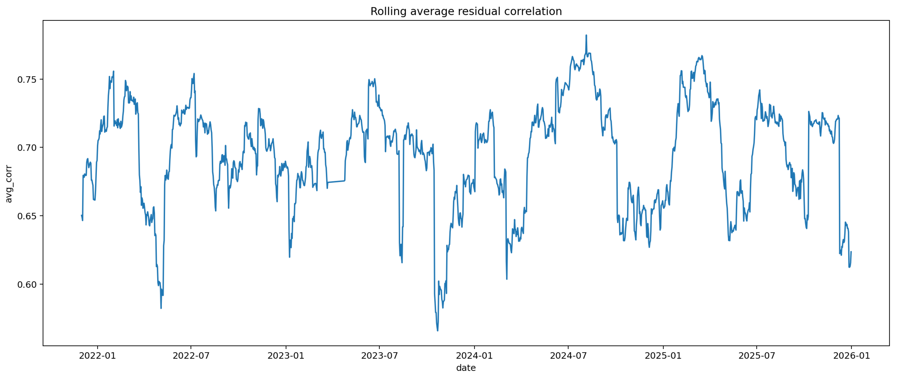
Figure A2.
Rolling Frobenius shift of the residual dependence matrix.
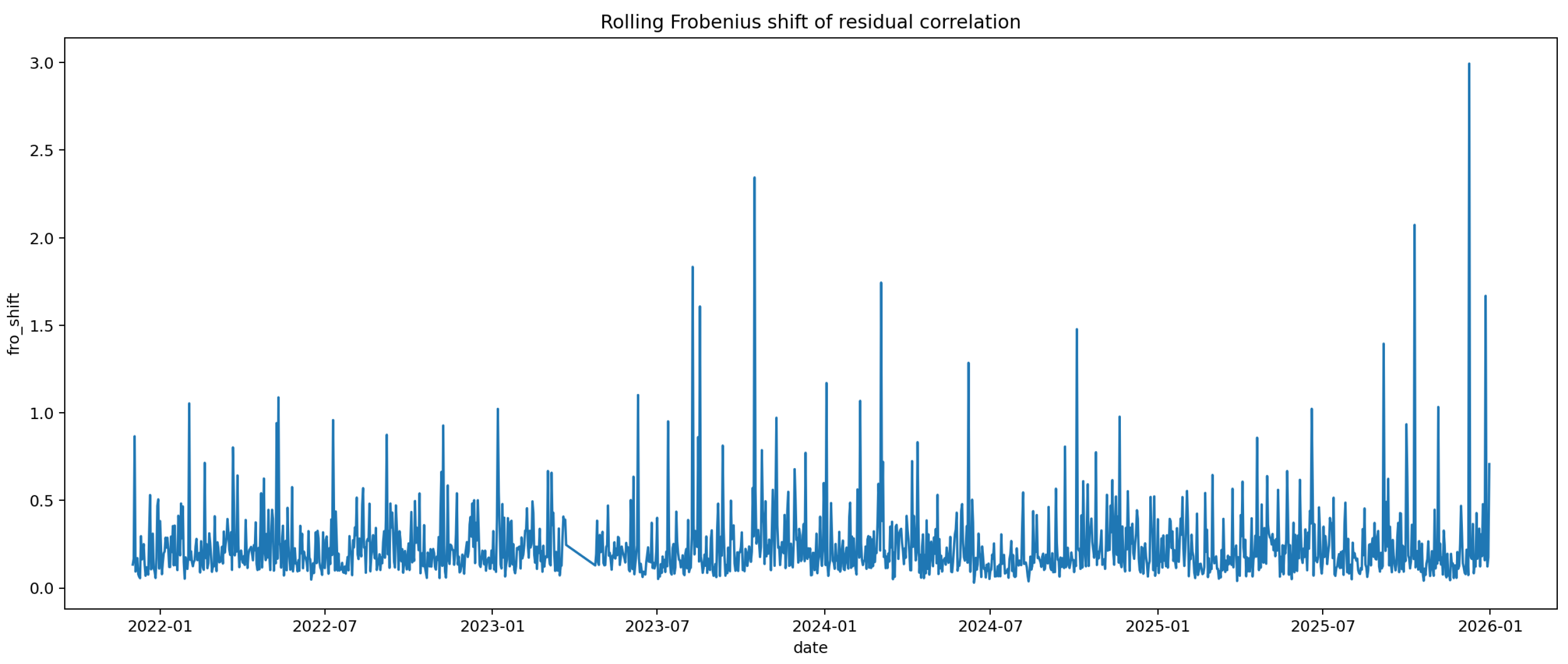
Appendix D. Additional Signature and Placebo Evidence
Figure A3.
Standardized average residual-correlation signature.
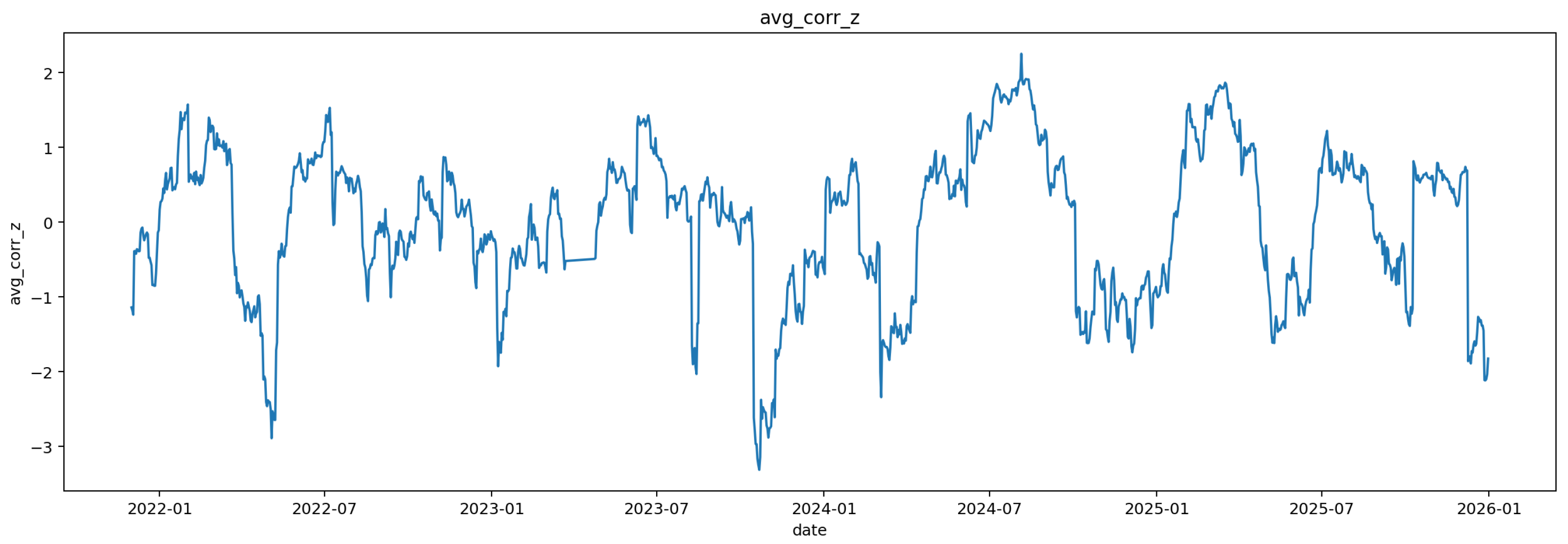
Figure A4.
Standardized Frobenius-type deformation signature.
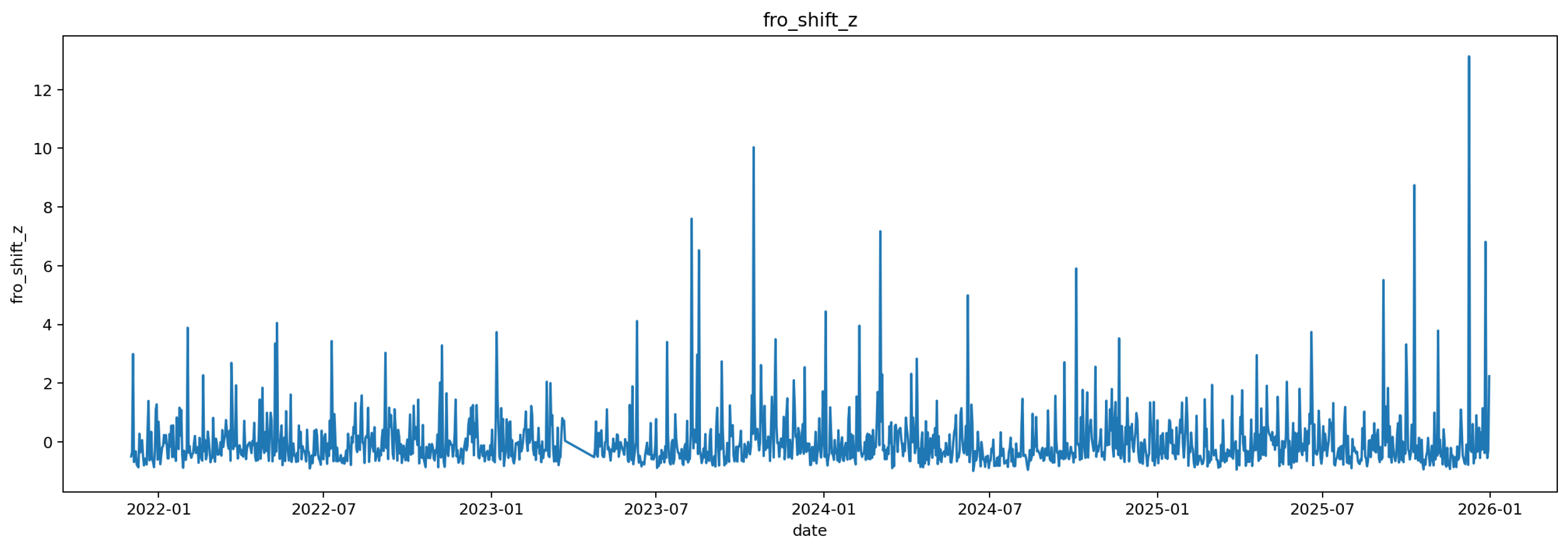
Figure A5.
Standardized influence-concentration signature.
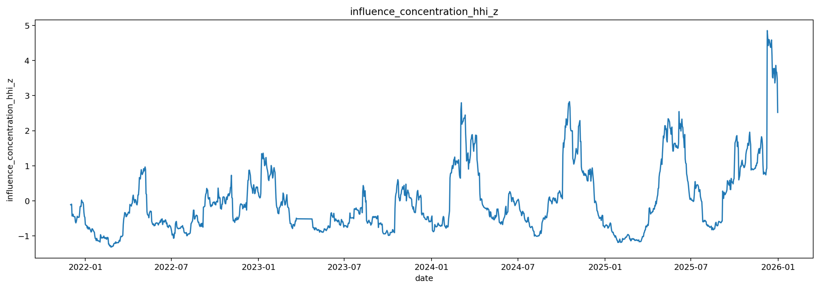
Figure A6.
Standardized influential-set-turnover signature.
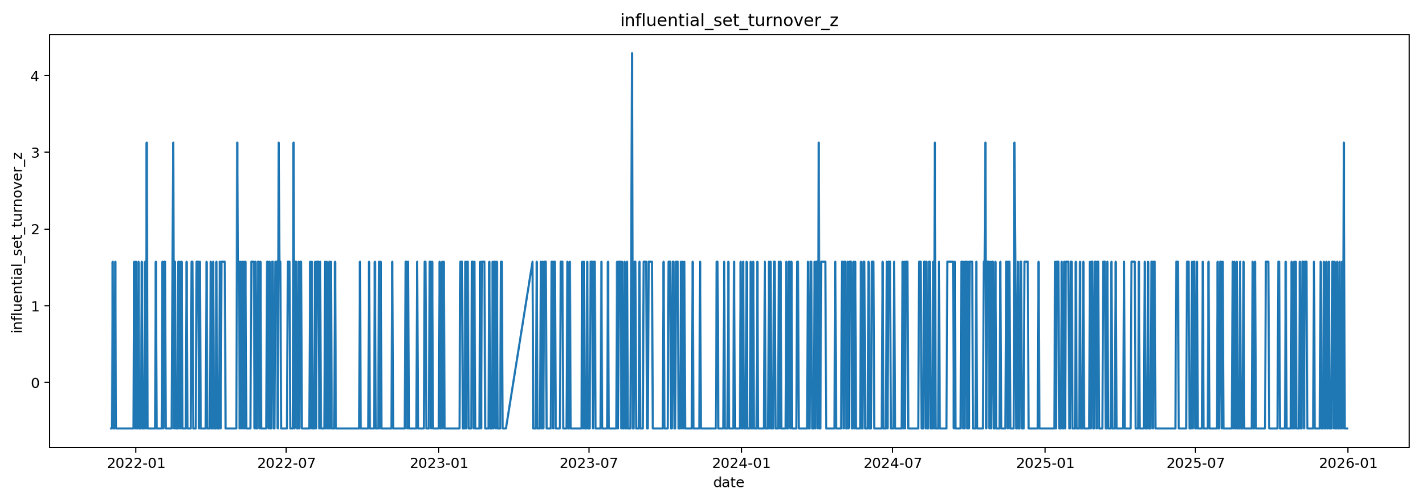
Figure A7.
Block-permutation placebo distribution. The dashed line marks the realized gain.
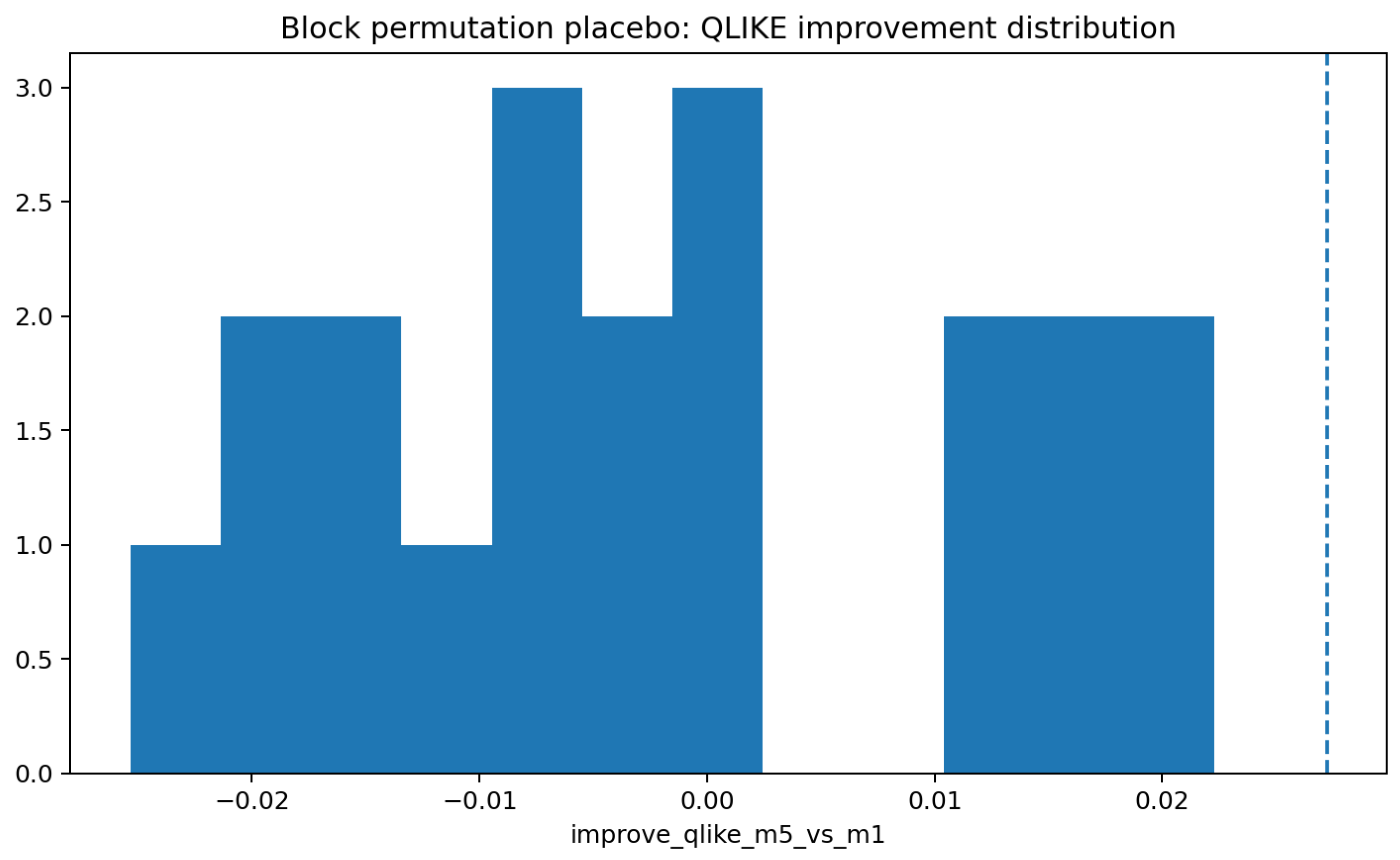
Figure A8.
Actual target versus HAR and deformation-only forecasts.
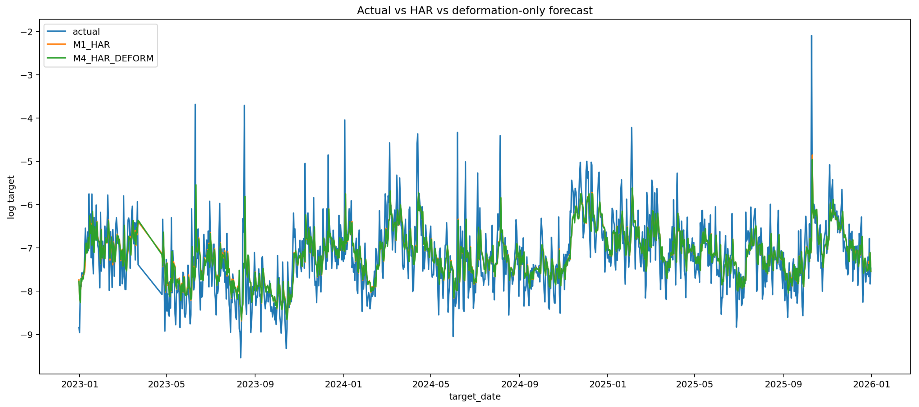
References
- Ahmed, M.S.; El-Masry, A.A.; Al-Maghyereh, A.I.; Kumar, S. Cryptocurrency Volatility: A Review, Synthesis, and Research Agenda. Res. Int. Bus. Financ. 2024, 71, 102472. [Google Scholar] [CrossRef] [Scilit]
- Ftiti, Z.; Louhichi, W.; Ben Ameur, H. Cryptocurrency Volatility Forecasting: What Can We Learn from the First Wave of the COVID-19 Outbreak? Ann. Oper. Res. 2023, 330, 665–690. [Google Scholar] [CrossRef] [Scilit] [PubMed]
- Feng, L.; Qi, J.; Lucey, B. Enhancing Cryptocurrency Market Volatility Forecasting with Daily Dynamic Tuning Strategy. Int. Rev. Financ. Anal. 2024, 94, 103239. [Google Scholar] [CrossRef] [Scilit]
- Brauneis, A.; Sahiner, M. Crypto Volatility Forecasting: Mounting a HAR, Sentiment, and Machine Learning Horserace. Asia-Pac. Financ. Mark. 2026, 33, 379–411. [Google Scholar] [CrossRef] [Scilit]
- Ji, Q.; Bouri, E.; Lau, C.K.M.; Roubaud, D. Dynamic Connectedness and Integration in Cryptocurrency Markets. Int. Rev. Financ. Anal. 2019, 63, 257–272. [Google Scholar] [CrossRef] [Scilit]
- Guo, L.; Sang, B.; Tu, J.; Wang, Y. Cross-Cryptocurrency Return Predictability. J. Econ. Dyn. Control 2024, 163, 104863. [Google Scholar] [CrossRef] [Scilit]
- Andersen, T.G.; Bollerslev, T.; Diebold, F.X.; Labys, P. Modeling and Forecasting Realized Volatility. Econometrica 2003, 71, 579–625. [Google Scholar] [CrossRef] [Scilit]
- Corsi, F. A Simple Approximate Long-Memory Model of Realized Volatility. J. Financ. Econom. 2009, 7, 174–196. [Google Scholar] [CrossRef] [Scilit]
- Qiu, Y.; Wang, Z.; Xie, T.; Zhang, X. Forecasting Bitcoin Realized Volatility by Exploiting Measurement Error under Model Uncertainty. J. Empir. Financ. 2021, 62, 179–201. [Google Scholar] [CrossRef] [Scilit]
- Barndorff-Nielsen, O.E.; Kinnebrock, S.; Shephard, N. Measuring Downside Risk – Realised Semivariance. In Volatility and Time Series Econometrics: Essays in Honor of Robert F. Engle; Bollerslev, T., Russell, J., Watson, M., Eds.; Oxford University Press: Oxford, UK, 2010; pp. 117–137. [Google Scholar]
- Maki, D. Forecasting Downside and Upside Realized Volatility: The Role of Asymmetric Information. J. Econ. Asymmetries 2024, 29, e00357. [Google Scholar] [CrossRef] [Scilit]
- Patton, A.J. Volatility Forecast Comparison Using Imperfect Volatility Proxies. J. Econom. 2011, 160, 246–256. [Google Scholar] [CrossRef] [Scilit]
- Mantegna, R.N. Hierarchical Structure in Financial Markets. Eur. Phys. J. B 1999, 11, 193–197. [Google Scholar] [CrossRef] [Scilit]
- Diebold, F.X.; Yılmaz, K. On the Network Topology of Variance Decompositions: Measuring the Connectedness of Financial Firms. J. Econom. 2014, 182, 119–134. [Google Scholar] [CrossRef] [Scilit]
- Ji, Q.; Bouri, E.; Kristoufek, L.; Lucey, B. Realised Volatility Connectedness among Bitcoin Exchange Markets. Financ. Res. Lett. 2021, 38, 101391. [Google Scholar] [CrossRef] [Scilit]
- Nguyen, A.P.N.; Mai, T.T.; Bezbradica, M.; Crane, M. Volatility and Returns Connectedness in Cryptocurrency Markets: Insights from Graph-Based Methods. Phys. A Stat. Mech. Its Appl. 2023, 632, 129349. [Google Scholar] [CrossRef] [Scilit]
- Poddar, A.; Misra, A.K.; Mishra, A.K. Return Connectedness and Volatility Dynamics of the Cryptocurrency Network. Financ. Res. Lett. 2023, 58, 104334. [Google Scholar] [CrossRef] [Scilit]
- Zhou, F.; Guo, W. Time-Varying Network Structure and Volatility Prediction in the Cryptocurrency Market. Financ. Res. Lett. 2026, 87, 109028. [Google Scholar] [CrossRef] [Scilit]
- Andersen, T.G.; Bollerslev, T.; Diebold, F.X.; Ebens, H. The Distribution of Realized Stock Return Volatility. J. Financ. Econ. 2001, 61, 43–76. [Google Scholar] [CrossRef] [Scilit]
- Patton, A.J.; Sheppard, K. Good Volatility, Bad Volatility: Signed Jumps and the Persistence of Volatility. Rev. Econ. Stat. 2015, 97, 683–697. [Google Scholar] [CrossRef] [Scilit]
- Engle, R. Dynamic Conditional Correlation: A Simple Class of Multivariate GARCH Models. J. Bus. Econ. Stat. 2002, 20, 339–350. [Google Scholar] [CrossRef] [Scilit]
- Ledoit, O.; Wolf, M. Honey, I Shrunk the Sample Covariance Matrix. J. Portf. Manag. 2004, 30, 110–119. [Google Scholar] [CrossRef] [Scilit]
- Bollerslev, T.; Patton, A.J.; Quaedvlieg, R. Exploiting the Errors: A Simple Approach for Improved Volatility Forecasting. J. Econom. 2016, 192, 1–18. [Google Scholar] [CrossRef] [Scilit]
- MacKinlay, A.C. Event Studies in Economics and Finance. J. Econ. Lit. 1997, 35, 13–39. [Google Scholar]
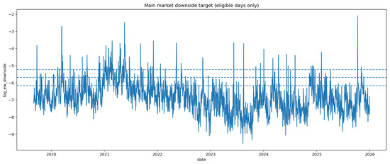
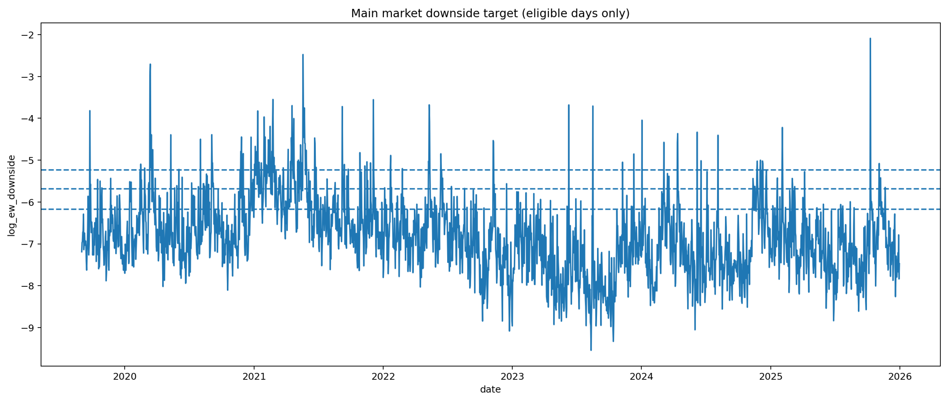
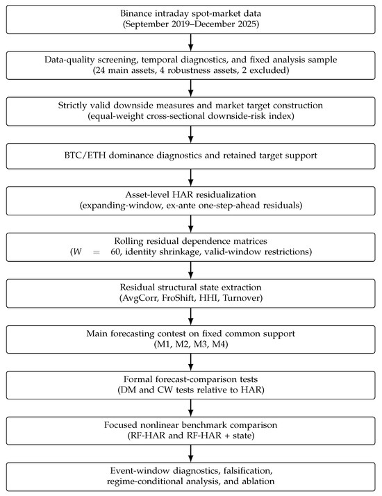
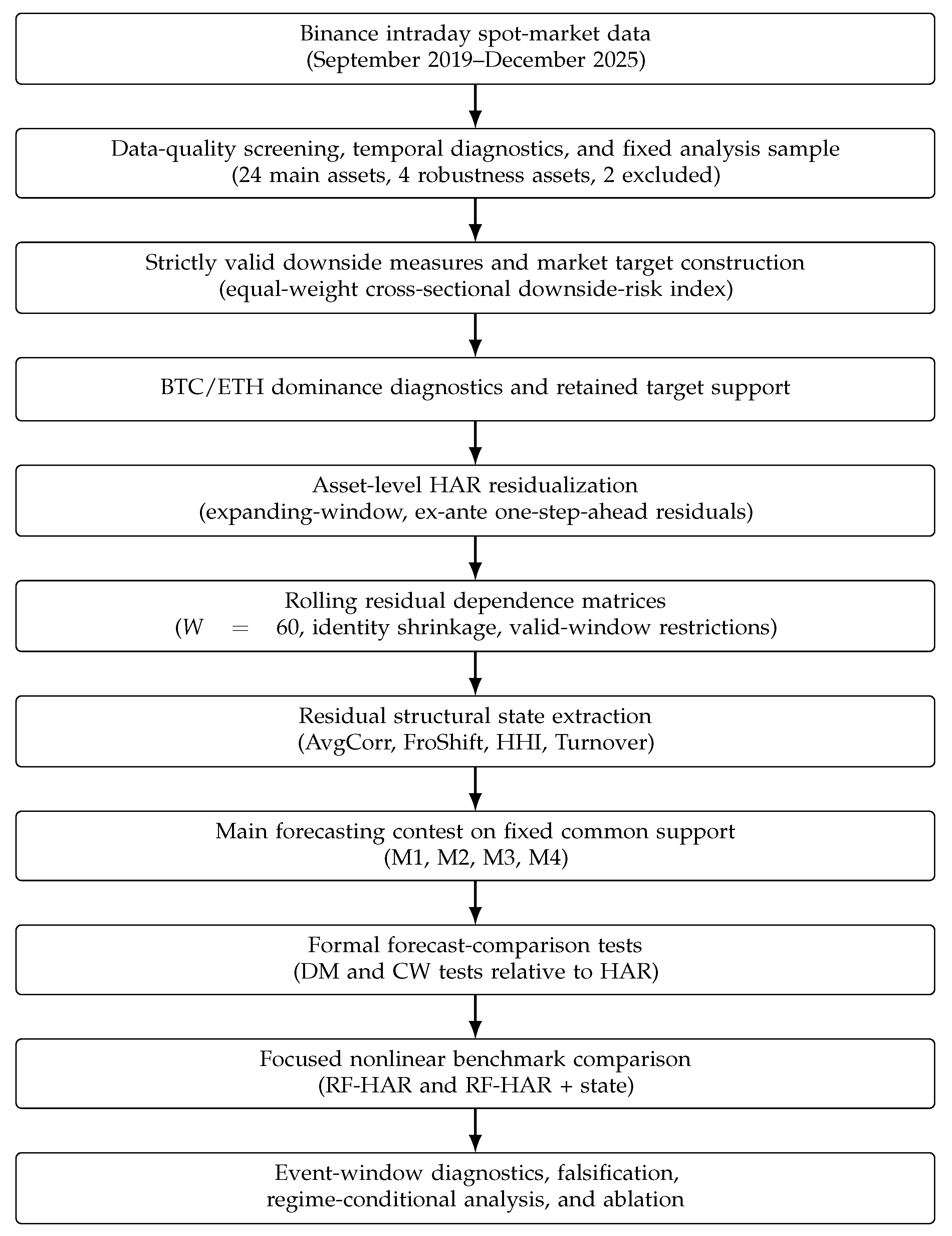
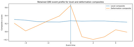
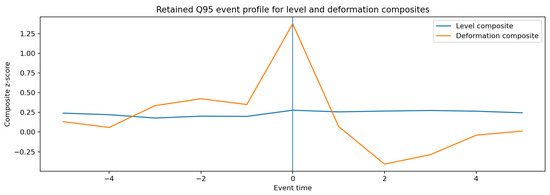
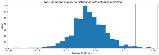
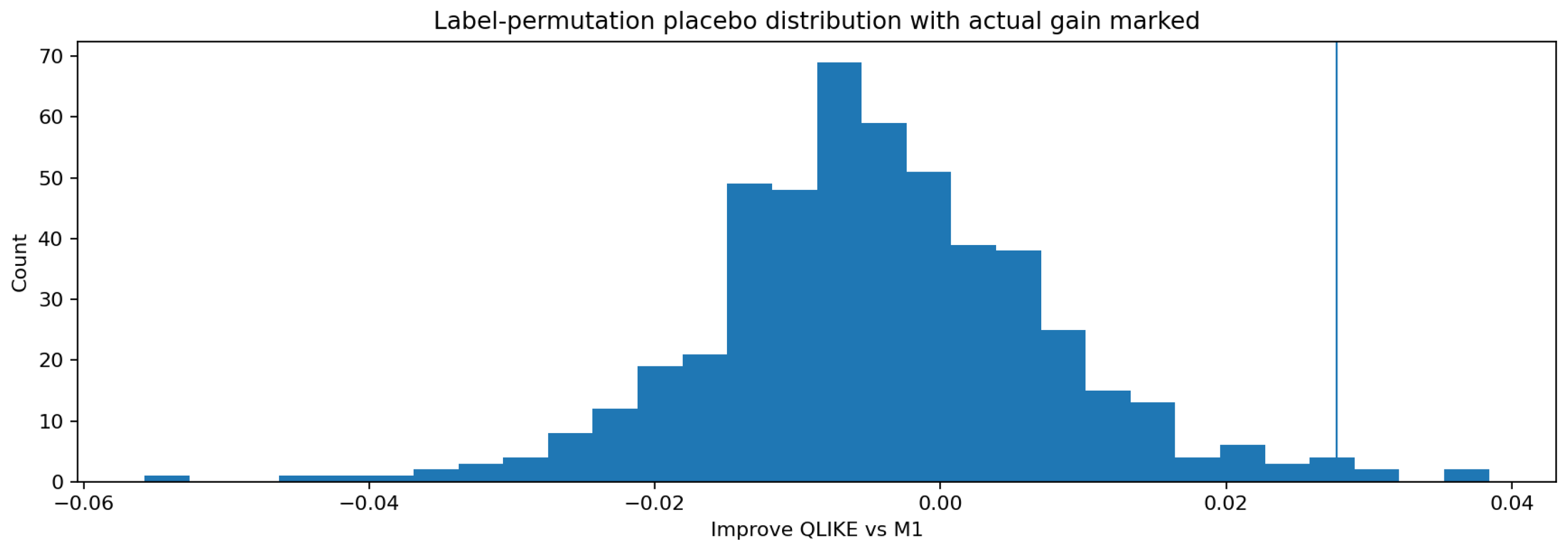
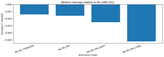
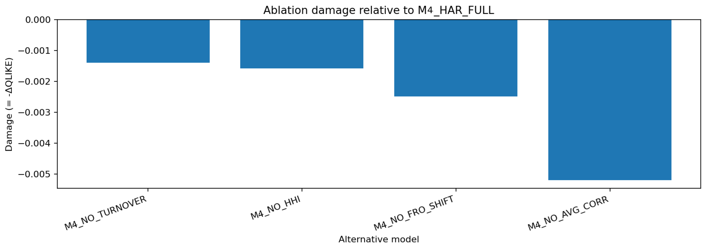

Disclaimer/Publisher’s Note: The statements, opinions and data contained in all publications are solely those of the individual author(s) and contributor(s) and not of MDPI and/or the editor(s). MDPI and/or the editor(s) disclaim responsibility for any injury to people or property resulting from any ideas, methods, instructions or products referred to in the content. |
© 2026 by the authors. Licensee MDPI, Basel, Switzerland. This article is an open access article distributed under the terms and conditions of the Creative Commons Attribution (CC BY) license.