A Causality-Guided Graph Framework for National AI Competitiveness Assessment, Forecasting, and Multi-Objective Fund Allocation

Abstract

As artificial intelligence (AI) increasingly reshapes the global technological and economic landscape, understanding and forecasting national AI competitiveness has become an important yet challenging task. Unlike conventional Analytic Hierarchy Process (AHP)–Entropy-based evaluation methods and machine learning approaches that treat indicators as isolated or weakly connected features, this study proposes an integrated framework that explicitly represents inter-indicator dependencies as a structured global topology. Based on an Input–Process–Output–Environment (IPOE) system with 24 indicators for 10 major economies during 2016–2025, AHP–Entropy, XGBoost, Design of Experiments (DOE), and Bayesian networks are combined to identify dependency pathways among indicators. These structural relations are embedded into a graph neural network (GNN) for competitiveness assessment, while a Dynamic GNN-ARIMA module is developed to project future competitiveness trajectories under limited samples. Building on these projections, a multi-objective fund allocation optimization model is constructed and solved via the NSGA-II algorithm to reduce policy volatility while maintaining future AI competitiveness with a strategic investment of RMB 500 billion. Results show that the U.S. remains the clear leader, followed by China, while mid-tier economies show noticeable reshuffling. Under the Min-Variance strategy with the investment, China is projected to significantly narrow the gap with the United States, reaching a comparable level of competitiveness.

1. Introduction

AI is no longer merely a tool for enhancing efficiency but has become a strategic core technology that profoundly impacts national sovereignty, economic security and long-term development [1,2]. Unlike previous technological revolutions, the strategic advantage of AI does not stem solely from breakthroughs in algorithms, but rather from the systematic synergy of multiple factors including computing power, data, talent, and institutional environments [3,4]. Against this backdrop, national AI competitiveness has emerged as a central focal point in global technological competition and geopolitical rivalry. Since 2023, the United States, the European Union, and China have successively released relevant strategic plans [5,6], indicating that AI competitiveness has become a crucial indicator of a nation’s comprehensive strength [7,8]. Currently, large models and computing infrastructure exhibit pronounced centralization trends. This not only widens the global technological benefit distribution gap economically but also profoundly reshapes the competitive landscape of national technological security at the strategic level [9,10]. Therefore, scientifically assessing and forecasting the development trends of national AI competitiveness holds significant theoretical value and provides decision support for policymakers to optimize strategic resource allocation.

However, quantitative indicators of national AI competitiveness undergo real-time fluctuations, fundamentally representing a complex system problem involving the coupling of multiple factors [11]. This perspective is also consistent with recent socio-technical research, which suggests that the performance and value realization of AI depend not only on technological inputs, but also on the interaction among organizational, institutional, and systemic conditions [12]. From this viewpoint, national AI competitiveness should be understood as a socio-technical system driven by nonlinear interactions among these variables, rather than as a purely technical outcome. For instance, input factors such as investment amount and GPU capabilities directly impact software development activity and AI talent migration processes, subsequently affecting innovation outcomes like AI publications count and AI patents count, ultimately forming an interconnected coupling network. When confronted with such complex issues, traditional machine learning methods like Support Vector Machines (SVMs) and Random Forests, along with conventional deep learning models such as Convolutional Neural Networks (CNNs), struggle to effectively capture these implicit causal dependencies, compromising modeling accuracy [13,14]. Simultaneously, the scarcity of AI competitiveness-related data further constrains the reliability of traditional methods. Against this backdrop, how to achieve dynamic assessment and trend forecasting of AI competitiveness under small-sample constraints has become a critical challenge requiring breakthroughs in this field.

In the field of holistic assessment of complex systems, existing research has already conducted certain explorations and practices in areas such as national comprehensive strength and innovation capabilities. For example, Al-Marzouqi et al. (2024) conducted a comparative analysis of major global AI indices [15]. The study noted that due to significant differences in metric selection and weighting, various assessment systems often yield markedly divergent evaluations for the same country, directly undermining the scientific rigor and practical decision-making value of existing indices. Moreover, in 2025, Doshi et al. explored the application of generative AI in strategic decision-making evaluations, confirming the limitations of single-AI assessments but demonstrating that aggregated multi-dimensional results achieved high similarity with human expert rankings [16]. In constructing composite indices, hybrid weighting models combining AHP and entropy weighting gained widespread adoption to balance expert knowledge with data objectivity [17,18,19,20]. For instance, Dong et al. in 2021 constructed an international competitiveness evaluation index system for the AI industry based on the Diamond Model, using China, the US, the UK, and Germany as case studies [21]. Combining the positive-negative ideal point weighting method with the simulated annealing algorithm to determine indicator weights, the study employed the TOPSIS method for comprehensive evaluation and ranking. This analysis examined the strengths, weaknesses, and underlying causes of each country’s AI industry competitiveness. In recent years, machine learning algorithms such as random forests and SVM have demonstrated significant advantages in nonlinear fitting tasks. They effectively capture complex data correlations, adapt to diverse data distributions, and provide efficient support for multidimensional quantitative analysis [22,23,24]. Ma et al. (2023) [25] constructed a multidimensional Global Smart Innovation Index and innovatively employed machine learning algorithms like random forests to automatically learn indicator weights from data, quantitatively assessing the smart innovation levels of 101 countries. Furthermore, Chun et al. in 2024 [26] explored key factors influencing AI technology specialization. They assessed countries’ technological specialization levels using the Revealed Comparative Advantage Matrix and empirically analyzed the linear relationship between AI technology specialization and national competitiveness through a panel regression model. For evaluating large-scale complex criteria, Garcia-Gastelum et al. (2025) proposed an AI program model integrating multiple methods for robust multi-criteria decision-making ranking, applying it to regional competitiveness analysis [27]. From a policy and sustainability perspective, Jin et al. (2025) [28] showed across 52 countries that expenditure decentralization and spending structure significantly shape sustainable development outcomes. Their results indicate that how public funds are allocated affects not only fiscal management, but also long-term national development performance.

Although existing methods have achieved certain progress in relevant fields, their direct application to national-level AI competitiveness assessments still faces numerous unavoidable limitations, thereby affecting the reliability and practical value of evaluation results [29]. Currently, research on national AI competitiveness evaluation predominantly relies on traditional machine learning and deep learning algorithms, as well as classical index methods such as the AHP and entropy weight method. Although some studies have attempted to incorporate innovative approaches like generative AI-based aggregation evaluation and multi-criteria robust ranking, significant limitations persist in practical implementation [10]. The most distinctive feature of national AI competitiveness lies in the highly coupled and complex topological relationships among multiple indicators. Traditional models often struggle to effectively capture these implicit causal dependencies, thereby constraining overall modeling accuracy [30,31]. Simultaneously, the scarcity of relevant real-world data further undermines the stability and credibility of traditional methods in practical evaluations. Therefore, the superimposition of these interconnected issues has rendered existing evaluation systems inadequate for accurately capturing the dynamic evolution of national AI competitiveness, thereby failing to effectively support the practical decision-making needs within policy formulation processes. To position the present study more clearly against representative prior work, a critical comparison of existing studies and the proposed framework is provided in Table 1.

Table 1. Comparison of representative studies and the proposed framework.

Study	Focus	Method	Strength	Limitation
Al-Marzouqi et al. (2024) [15]	AI index comparison	Descriptive comparison	Clarifies index differences	No unified model
Doshi et al. (2025) [16]	AI-assisted strategic evaluation	Generative AI aggregation	Improves evaluation consistency	No structural or forecasting framework
Dong et al. (2021) [21]	AI industry competitiveness	Weighting with TOPSIS	Interpretable country ranking	Static and linear
Ma et al. (2023) [25]	Smart innovation evaluation	Machine learning weighting	Captures nonlinear importance	Weak structural interpretability
Chun et al. (2024) [26]	AI specialization and competitiveness	RCA with panel regression	Strong econometric view	Not an integrated evaluation framework
Garcia-Gastelum et al. (2025) [27]	Robust multi-criteria ranking	AI-assisted MCDM	Strong ranking robustness	No dynamic prediction or optimization
This study	AI competitiveness assessment, forecasting, and allocation	Dynamic GNN-ARIMA forecasting with NSGA-II Multi-objective optimization	Integrated evaluation-forecasting-optimization pipeline	Limited by short annual samples

To address these challenges, this study develops an integrated graph-based framework for national AI competitiveness assessment, forecasting, and fund allocation. The framework combines structured indicator system construction, GNN modeling, forecasting with dynamic GNN-ARIMA, and policy-oriented multi-objective optimization within a unified pipeline. The main contributions of this paper are summarized as follows:

(a)

An IPOE-based indicator system is developed for national AI competitiveness evaluation. By organizing 24 indicators into the input, process, output, and environment dimensions, the system provides a structured basis for cross-country assessment and inter-indicator dependency analysis.

(b)

A dependency-aware forecasting model is developed by integrating graph-based structural refinement with dynamic GNN-ARIMA prediction. By explicitly encoding inter-indicator relationships as a structured global topology, the model improves the interpretability and structural consistency of competitiveness forecasting under limited samples.

(c)

An NSGA-II-based multi-objective optimization model is established for short-horizon fund allocation. By jointly optimizing future competitiveness and policy smoothness, the model provides an actionable strategy for national AI investment planning under a fixed budget scenario.

2. Methodological Framework and Data Preparation

2.1. Method Overview

This study develops an integrated framework for the evaluation, forecasting, and optimization of national AI competitiveness. The framework starts from an IPOE-based indicator system, where AI development is described from four dimensions: input, process, output, and environment. On this basis, a global country-year panel covering more than 200 countries over 2016–2025 is constructed for indicator weighting, nonlinear sensitivity analysis, and dependency learning. From this broader panel, 10 target countries are selected for the final static evaluation and dynamic forecasting analysis.

Indicator weighting is initialized by combining the AHP with the entropy method, so that expert judgment and data dispersion are both retained in the baseline weighting scheme. To supplement this linear aggregation, XGBoost is applied to perturbation-response samples generated from the indicator system and is used to measure the nonlinear sensitivity of the indicators. In parallel, DOE and Bayesian networks are used to characterize interaction effects and dependency pathways among the indicators. The resulting weights and structural relations provide the prior information for the subsequent graph-based evaluation model.

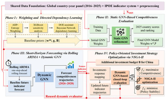
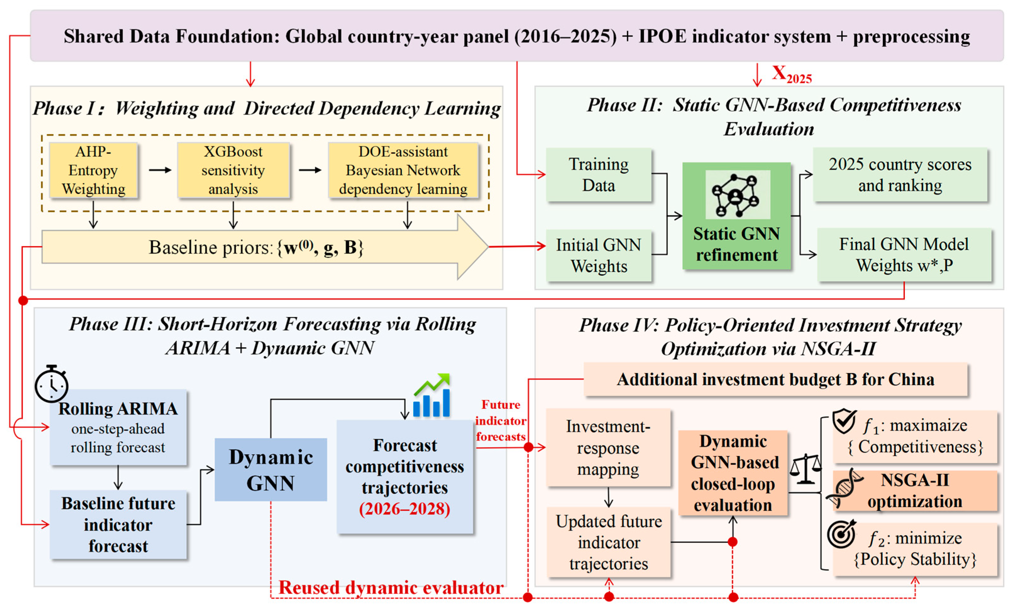
For the static assessment task, the prior weights and dependency structure are embedded into a graph neural network to derive the 2025 competitiveness scores of the ten countries. For the dynamic analysis, each indicator series is first modeled by ARIMA for short-horizon forecasting over 2026–2028. To mitigate the reliability concerns associated with direct long-range extrapolation from a short annual sample, the forecasting module is implemented in a one-step-ahead rolling manner: at each stage, only the next year is forecast, and the predicted indicator values are then fed into the graph-based scoring framework to update the system state before proceeding to the following year. Finally, under the additional investment budget assigned to China, a multi-objective optimization model is used to balance competitiveness improvement and policy stability over the same short planning horizon. The overall workflow of the proposed study is illustrated in Figure 1.

Figure 1. Overall workflow of the proposed framework.

2.2. Data Collection and Preprocessing

2.2.1. Data Collection

The full dataset is constructed as a global country-year panel covering more than 200 countries over the period 2016–2025. The 24 sub-indicators are organized under the IPOE framework, and their detailed definitions are reported in Table 2. For the final static evaluation and dynamic forecasting analysis, 10 target countries are selected, namely the United States, China, the United Kingdom, Germany, South Korea, Japan, France, Canada, the United Arab Emirates, and India.

Table 2. IPOE Tiered Indicator System for National AI Competitiveness Evaluation.

Dimension	Abbreviation	Full Indicator Name
Input	Inv. Amt.	Investment Amount
	GPU Cap.	GPU Capabilities
	GDP	Gross Domestic Product
	Energy	Energy Supply
	Data Trf.	Data Traffic
	5G Cov.	5G Coverage Rate
	Opn.	Openness Index
Process	SO Dev.	Software Development Activity
	AI Pen.	AI Penetration Rate
	AI Hire	AI Hiring Rate
	AI Migr.	AI Talent Migration
	AI Conc.	AI Concentration
Output	Patents	AI Patents Count
	Pubs.	AI Publications Count
	Lg. AI Sys.	Large AI Systems Count
	Pats/M	Patents per Million People
	Pubs/M	Publications per Million People
	OSS Infl.	Open Source Software Influence
	Corp. AI	Corporate AI Adoption Rate
	AI Index	AI Composite Index
Environment	AI Laws	AI Regulatory Laws Count
	Intl. Coop.	International Cooperation Index
	Glob.	Globalization Index
	Biz. Risk	Business Risk Index

The raw data were collected from multiple public sources, including the Stanford HAI AI Index Report 2025 [32], EPOCH AI, the World Bank Group [33], DataCommons [34], the Center for Security [35] and Emerging Technology (CSET) [36], and the LMArena platform [37]. All observations were organized at the country-year level. The corresponding source websites are provided in Appendix A, Table A1.

Let $d_{i,j,t}$ denote the raw value of indicator $\mathrm{j}$ for country $i$ in year $t$, where $i=1, 2,\dots , N_{\mathrm{all}}$, $j=1, 2,\dots , 24$, and $t=2016, 2017,\dots , 2025$. Here, $N_{\mathrm{all}}$ denotes the total number of countries in the full panel. The raw dataset can then be written as $D=\left\{d_{i,j,t}\right\}$.

2.2.2. Data Preprocessing

Because the indicators were compiled from heterogeneous sources, preprocessing was performed before model construction.

Records with missing country labels, missing year labels, or duplicated country-year entries were removed. For quantitative indicators with unavailable observations, missing entries were completed using constrained multivariate iterative imputation with a Bayesian Ridge estimator. Imputation was applied only to originally missing cells, whereas observed zeros were retained. To preserve domain consistency, post-imputation values were constrained to feasible ranges, and count-type indicators were rounded to integers when appropriate. The imputation procedure was applied across all 24 quantitative indicators in the IPOE system.

After imputation, all indicators were direction-aligned so that larger values uniformly indicate stronger AI competitiveness. Benefit-type indicators retained their original direction, whereas cost-type indicators were reversed before transformation. In particular, the Business Risk Index was treated as a cost-type indicator.

Since the subsequent modules require different numerical representations, two transformed panels were constructed. For the entropy-based objective weighting in Section 3.2, a nonnegative rescaled value ${\overline{\mathrm{x}}}_{\mathrm{i},\mathrm{j},\mathrm{t}}\in \left[0,100\right]$ was defined from the direction-aligned value ${\mathrm{r}}_{\mathrm{i},\mathrm{j},\mathrm{t}}$ as

$${\overline{x}}_{i,j,t}=100\times {\displaystyle \frac{r_{i,j,t}-r_j^{\min }}{r_j^{\max }-r_j^{\min }}},$$

(1)

where

$$r_j^{\min }=\underset{i,t}{\min }{r}_{i,j,t},\hspace{1em}{r}_j^{\max }=\underset{i,t}{\max }{r}_{i,j,t}.$$

(2)

If $r_j^{\max }=r_j^{\min }$, indicator $\mathrm{j}$ contains no discriminatory information over the historical window and is removed from the subsequent analysis.

For the graph-based evaluation, ARIMA forecasting, and investment optimization modules in Section 4 and Section 5, a training-derived standardized representation was further constructed as

$$x_{i,j,t}={\displaystyle \frac{{\overline{x}}_{i,j,t}-{\mu }_j}{{\sigma }_j}},$$

(3)

where ${\mu }_j$ and ${\sigma }_j$ denote the mean and standard deviation of the nonnegative rescaled indicator ${\overline{x}}_{i,j,t}$ for indicator $\mathrm{j}$, estimated from the global historical panel over 2016–2025. These statistics are held fixed and applied unchanged in Section 4 and Section 5.

The nonnegative rescaled representation ${\overline{x}}_{i,j,t}$ is used in the entropy-based weighting step, whereas the standardized representation ${\mathrm{x}}_{\mathrm{i},\mathrm{j},\mathrm{t}}$ is used in the graph-based evaluation, forecasting, and optimization modules.

After preprocessing, the standardized feature matrix for year $\mathrm{t}$ is denoted by $X_t=\left[x_{i,j,t}\right]$, which serves as the common input to the graph construction, ranking, forecasting, and optimization modules. The nonnegative rescaled panel ${\tilde{X}}_t=\left[{\tilde{x}}_{i,j,t}\right]$ is used only in the entropy-based weighting step.

3. IPOE Indicator System and Hybrid Weighting Mechanism

3.1. Framework Overview and Indicator System

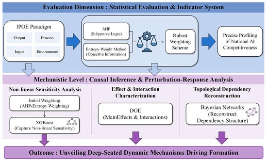
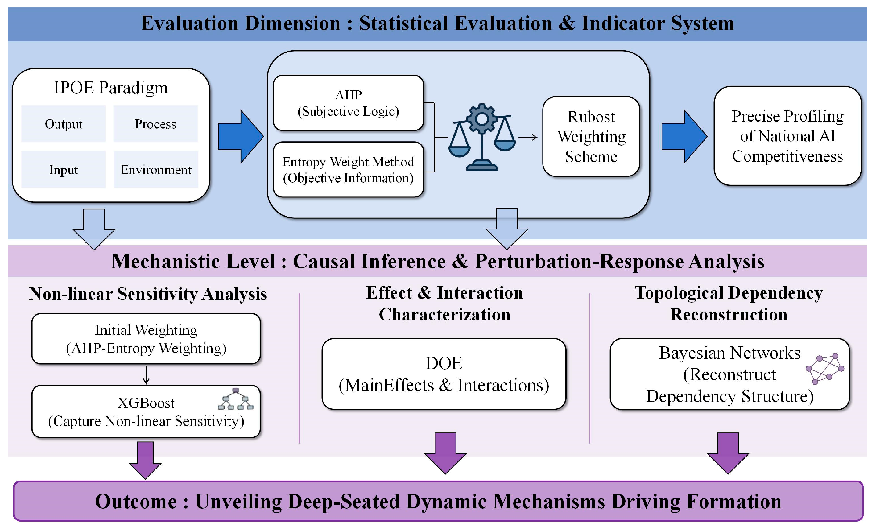
Figure 2 presents the weighting and dependency identification framework used in the evaluation stage. The evaluation of national AI competitiveness starts from an IPOE-based hierarchical indicator system. The system contains four dimensions, namely Input, Process, Output, and Environment, and 24 sub-indicators, as summarized in Table 2.

Figure 2. Framework for indicator weighting and dependency identification in the national AI competitiveness evaluation system.

The Input dimension describes the basic resources that support AI development, including capital, computing capacity, energy, data, and digital infrastructure. The Process dimension characterizes the transformation of these resources into technological activity and talent dynamics. The Output dimension reflects scientific, technological, and industrial achievements generated by the AI system. The Environment dimension captures the institutional and external conditions under which AI development takes place, including regulation, international cooperation, globalization, and business risk. In this classification, AI Regulatory Laws Count is treated as an environmental indicator rather than an output indicator.

The IPOE structure is used not only for indicator organization, but also as a prior ordering constraint in the dependency analysis developed in Section 3.4.

3.2. AHP–Entropy Integrated Weighting Model

To aggregate the nonnegative rescaled indicators into a baseline weighting scheme, a hybrid weighting model combining the AHP and the entropy method is adopted. The entropy component is computed on the rescaled panel $\overline{\mathrm{X}}$, whereas the graph-based evaluation, forecasting, and optimization modules in Section 4 and Section 5 use the standardized panel $\mathrm{X}$. The composite score of country i is defined as

$$y_{i,t}^{\left(0\right)}={\displaystyle {\displaystyle \sum }_{j=1}^M}{w}_j{\overline{x}}_{i,j,t},\hspace{1em}{w}_j\ge 0,\hspace{1em}{\displaystyle {\displaystyle \sum }_{j=1}^M}{w}_j=1,$$

(4)

where $w_j$ denotes the integrated weight of indicator j.

The subjective component is obtained by AHP. For each hierarchical layer, a pairwise comparison matrix

$$A=\left(a_{uv}\right)\in {\mathrm{R}}^{h\times h}$$

(5)

is constructed, where h is the number of factors in the corresponding layer. The pairwise-comparison matrices were elicited from K domain experts with backgrounds in AI policy, industrial economics, and intelligent systems. When multiple expert judgments were available, the entrywise geometric mean was used to construct the aggregated matrix. Let r be the eigenvector associated with the maximum eigenvalue ${\lambda }_{\max }$. The subjective weight is then given by

$${\mathrm{w}}_{\mathrm{u}}^{\left(\mathrm{s}\right)}={\displaystyle \frac{r_u}{{{\displaystyle \sum }}_{\mathrm{v}=1}^{\mathrm{h}}{\mathrm{r}}_{\mathrm{v}}}}.$$

(6)

Consistency is evaluated by

$$\mathrm{CI}={\displaystyle \frac{{\lambda }_{\max }-h}{h-1}},\mathrm{CR}={\displaystyle \frac{\mathrm{CI}}{\mathrm{RI}}},$$

(7)

where RI is the random index. The judgment matrix is regarded as acceptably consistent when $\mathrm{CR}<0.1.$

The objective component is obtained by the entropy method on the nonnegative rescaled panel $\overline{X}$ defined in Section 2.2.2. This treatment preserves the nonnegativity required by entropy-based weighting while avoiding pseudo-zero inflation in sparse indicators. For indicator j, define

$$p_{i,j,t}={\displaystyle \frac{{\overline{x}}_{i,j,t}}{{{\displaystyle \sum }}_{i=1}^{N_{\mathrm{all}}}{{\displaystyle \sum }}_{t=2016}^{2025}{\overline{x}}_{i,j,t}}}.$$

(8)

For the retained indicators, the preprocessing step in Section 2.2.2 ensures that

$${\displaystyle {\displaystyle \sum }_{i=1}^{N_{\mathrm{all}}}}{\displaystyle {\displaystyle \sum }_{t=2016}^{2025}}{\overline{x}}_{i,j,t}>0,$$

(9)

so the above proportion is well defined. The entropy of indicator j is

$$e_j=-{\displaystyle \frac{1}{\ln \left(N_{\mathrm{all}}{T}_h\right)}}{\displaystyle {\displaystyle \sum }_{i=1}^{N_{\mathrm{all}}}}{\displaystyle {\displaystyle \sum }_{t=2016}^{2025}}{p}_{i,j,t}\ln p_{i,j,t},\hspace{1em}{T}_h=10,$$

(10)

with the convention $0\ln 0=0$. The divergence coefficient is $d_j=1-e_j,$ and the corresponding objective weight is

$$w_j^{\left(o\right)}={\displaystyle \frac{d_j}{{{\displaystyle \sum }}_{k=1}^M{d}_k}}.$$

(11)

The final weight is defined by the convex combination

$$w_j=\lambda w_j^{\left(s\right)}+\left(1-\lambda \right)w_j^{\left(o\right)},\lambda \in \left[0,1\right].$$

(12)

In this study, $\lambda =0.5,$ reflecting the intention to give equal importance to expert knowledge and data dispersion in the absence of a priori evidence favoring either component. The resulting vector $w=\left(w_1,\dots ,w_M\right)$ serves as the baseline weighting scheme for the subsequent sensitivity and graph-based analyses.

3.3. Feature Importance Modeling via Cross-Validated XGBoost

To quantify how local perturbations of the baseline weighting scheme affect the composite evaluation system, a perturbation-response analysis is introduced, in which feasible perturbed weight vectors are mapped to the corresponding deviations in country-year scores. Let $w=\left(w_1,\dots ,w_M\right)$ be the baseline weight vector. For perturbation sample n, let $v_n=\left(v_{n,1},\dots ,v_{n,M}\right)$ denote a perturbed weight vector generated in the neighborhood of w, subject to

$$v_{n,j}\ge 0,{\displaystyle \sum }_{j=1}^M{v}_{n,j}=1.$$

(13)

Equation (13) defines a feasible perturbed weight vector on the probability simplex around the baseline weighting scheme.

Under $v_n$, the perturbed score of country i is

$$y_{i,t}^{\left(v_n\right)}={\displaystyle {\displaystyle \sum }_{j=1}^M}{v}_{n,j}{\overline{x}}_{i,j,t}.$$

(14)

The observed response of perturbation sample n is measured by the mean absolute deviation from the baseline scores:

$$r_n={\displaystyle \frac{1}{N_{\mathrm{all}}{T}_h}}{\displaystyle {\displaystyle \sum }_{i=1}^{N_{\mathrm{all}}}}{\displaystyle {\displaystyle \sum }_{t=2016}^{2025}}\left|y_{i,t}^{\left(v_n\right)}-y_{i,t}^{\left(w\right)}\right|.$$

(15)

where $y_{i,t}^{\left(w\right)}$ denotes the baseline country-year score induced by the baseline weight vector $\mathrm{w}$. This quantity serves as the response variable for XGBoost training.

The perturbation dataset is therefore ${\left\{\left({\mathrm{v}}_{\mathrm{n}},{\mathrm{r}}_{\mathrm{n}}\right)\right\}}_{\mathrm{n}=1}^{{\mathrm{N}}_{\mathrm{s}}},$ where $N_s$ is the number of generated perturbation samples. An XGBoost regressor is trained on this dataset under K-fold cross-validation. Its objective function is

$$\mathrm{L}={\displaystyle \sum }_{n=1}^{N_s}\mathrm{l}\left(r_n,{\widehat{r}}_n\right)+{\displaystyle \sum }_{k=1}^K\mathrm{\Omega }\left(f_k\right),$$

(16)

where ${\widehat{r}}_n$ is the predicted response of perturbation sample $n$, $r_n$ is the observed response defined in Equation (15), $\mathrm{l}\left(\cdot ,\cdot \right)$ is the loss function, and $\mathrm{\Omega }\left(f_k\right)$ is the regularization term of the $\mathrm{k}$-th tree.

The resulting feature importance scores are used to rank the indicators according to their nonlinear influence on the composite evaluation system. These scores are not used as direct replacements for the AHP–entropy weights; instead, they provide an additional data-driven measure of indicator sensitivity. The stability of these perturbation-based importance scores is further examined through a country-level bootstrap procedure in Section 6.2.

3.4. Causal Pathway Identification Based on DOE and Bayesian Networks

Single-indicator perturbation is insufficient for identifying joint effects among indicators. To describe dependency pathways more explicitly, DOE and Bayesian networks are used. The Bayesian network structure was learned from the observed country-year indicator panel, while the DOE module was used to support interaction screening and sensitivity characterization.

DOE is first employed to generate structured multi-indicator perturbation samples around the baseline weight vector. These samples provide the basis for analyzing interaction effects under controlled combinations of indicator changes. On this basis, a Bayesian network is introduced to represent the dependency structure among indicators.

Let $z=\left(z_1,z_2,\dots ,z_M\right)$ denote the random variables associated with the M indicators. The joint distribution is factorized as

$$\mathrm{P}\left(z_1,z_2,\dots ,z_M\right)={\displaystyle \prod }_{j=1}^M\mathrm{P}\left(z_j\mid \mathrm{Pa}\left(z_j\right)\right),$$

(17)

where $\mathrm{Pa}\left(z_j\right)$ denotes the parent set of node ${\mathrm{z}}_{\mathrm{j}}$.

The IPOE hierarchy is used as a partial-order prior in structure learning. In particular, edges from later stages to earlier stages are excluded, while edges within the same layer or between adjacent layers are retained only when supported by the data. This constraint improves interpretability and keeps the learned topology consistent with the mechanism of capability formation described by the IPOE framework.

After structure learning, the inferred dependency graph is represented by the adjacency matrix

$$B=\left[b_{u,v}\right], b_{u,v}=\{\begin{array}{cc}1,& \mathrm{if} u\to v \mathrm{is} \mathrm{retained},\\ 0,& \hspace{1em} \mathrm{otherwise}.\end{array}$$

(18)

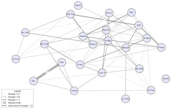
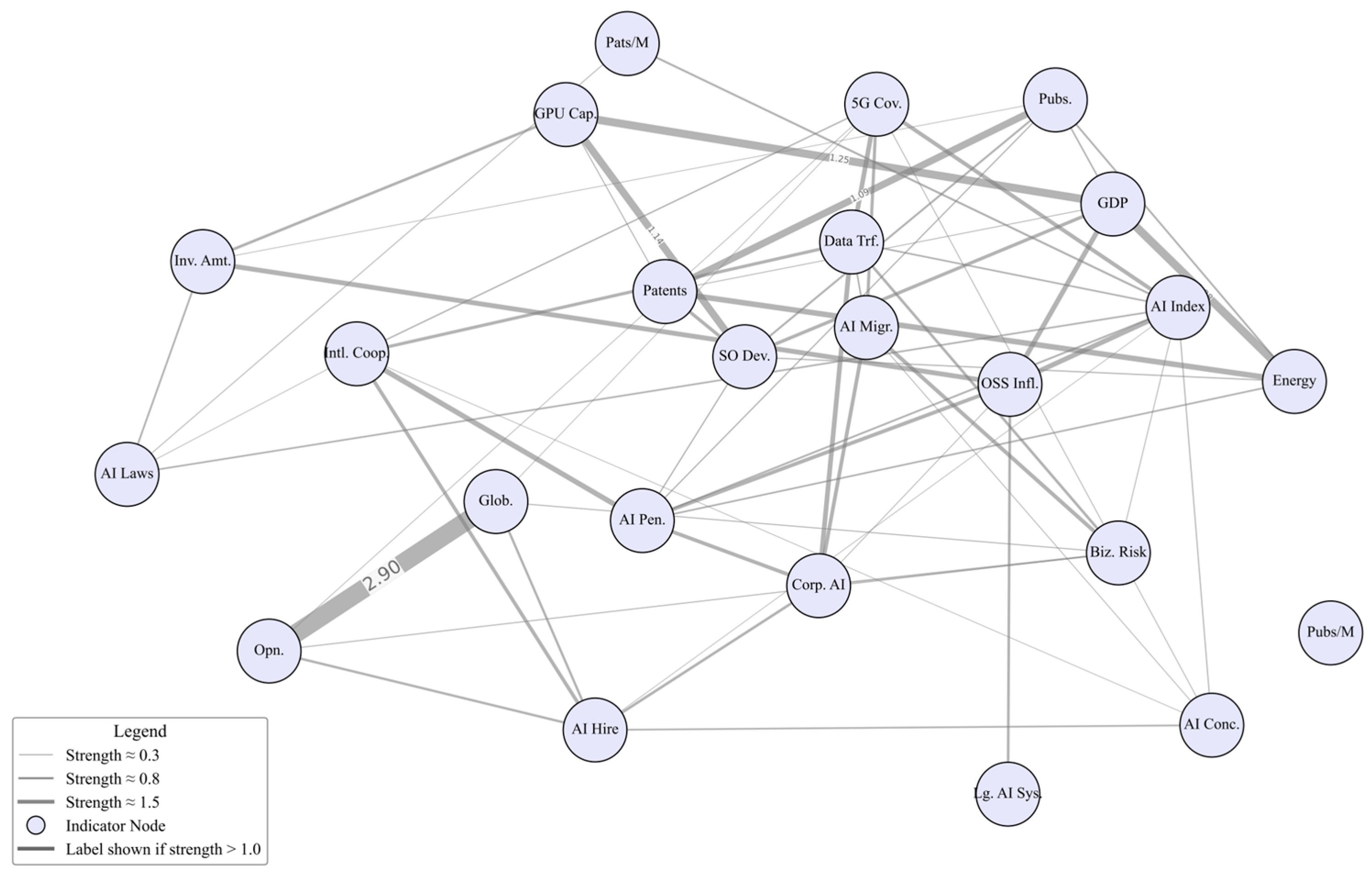
The learned network structure is shown in Figure 3. The matrix B is used as the structural prior for the graph-based evaluation model developed in the next section.

Figure 3. Inter-indicator Structural Pathways.

4. Competitiveness Evaluation and Dynamic Forecasting via GNN

Building on the hybrid weighting scheme and structural prior identified in Section 3, this section develops a graph-based framework for the evaluation and forecasting of national AI competitiveness. First, a static GNN-based evaluation model is constructed by embedding the directed inter-indicator dependency structure and prior importance information into a directed graph convolution framework, thereby generating refined indicator weights and the corresponding competitiveness ranking for the target year. On this basis, a dynamic forecasting model is further established by combining ARIMA-based indicator projection with a dynamic GNN module, so that the temporal evolution of indicator salience can be captured and short-term national AI competitiveness over 2026–2028 can be evaluated in a structured and consistent manner. To avoid unreliable direct long-horizon extrapolation, future states are generated recursively through rolling one-step-ahead updates rather than a single multi-year forecast [38].

4.1. Competitiveness Evaluation Model via GNN

4.1.1. Directed Topological Graph Construction

The dependency pathways learned in Section 3.4 are inherently directed. To preserve this causal orientation in the weight-refinement stage, the graph-based evaluation model is constructed on a directed structural prior rather than on a symmetrized graph. Let

$$B=\left[b_{u,v}\right]\in {\{0,1\}}^{M\times M}$$

(19)

denote the directed adjacency matrix inferred from the DOE-Bayesian network analysis, where $b_{u,v}=1$ if the directed edge $u\to v$ is retained, and $b_{u,v}=0$ otherwise. To incorporate self-dependence, define

$$\tilde{B}=B+I_M,$$

(20)

where $I_M$ is the $M\times M$ identity matrix. Since indicator $v$ should aggregate information from its retained directed predecessors, the in-degree of node $v$ is defined as

$${\widehat{d}}_v^{\mathit{in}}={\displaystyle {\displaystyle \sum }_{u=1}^M}{\tilde{b}}_{u,v},$$

(21)

and the corresponding diagonal matrix is

$${\tilde{D}}_{\mathit{in}}=\mathrm{diag}\left({\widehat{d}}_1^{\mathit{in}},\dots ,{\widehat{d}}_M^{\mathit{in}}\right)$$

(22)

The directed propagation matrix used in graph convolution is then defined as

$$P={\tilde{D}}_{\mathit{in}}^{-1}{\tilde{B}}^{\top }.$$

(23)

Under this construction, each node aggregates information only from its retained directed predecessors and itself, so that message passing follows the causal orientation identified in Section 3.4. Compared with undirected symmetrization, this directed formulation avoids reverse mixing from downstream indicators back to their upstream causes. The corresponding directed topology is illustrated in Figure 3.

4.1.2. GNN-Based Weight Refinement

Let $w^{\left(0\right)}={\left(w_1^{\left(0\right)},\dots ,w_M^{\left(0\right)}\right)}^{\mathrm{T}}$ denote the baseline AHP–entropy weight vector obtained in Section 3.2. Let $\iota ={({\iota }_1,\dots ,{\iota }_M)}^{\mathrm{T}}$ be the raw XGBoost importance scores obtained in Section 3.3, and define the normalized importance vector

$$g_j={\displaystyle \frac{{\iota }_j}{{{\displaystyle \sum }}_{k=1}^M{\iota }_k}},j=1,\dots ,M.$$

(24)

The initial node-feature matrix is then constructed as

$$H^{\left(0\right)}=\left[w^{\left(0\right)},g\right]\in {\mathrm{R}}^{M\times 2}.$$

(25)

Because no external ground-truth label of national AI competitiveness is available, the graph neural network is not used as a supervised predictor of country scores. Instead, it is used as a graph-regularized weight-refinement module that adjusts the baseline weights under the directed topological constraints encoded by $P$.

A one-layer graph convolution is adopted:

$$H^{\left(1\right)}=\mathrm{\sigma }\left(P{H}^{\left(0\right)}{W}_1+1b_1^{\top }\right),$$

(26)

where P is the directed propagation matrix defined in Section 4.1.1, $W_1\in {\mathrm{R}}^{2\times q}$ and $b_1\in {\mathrm{R}}^q$ are learnable parameters, q is the hidden dimension, $1\in {\mathrm{R}}^M$ is the all-ones vector, and $\mathrm{\sigma }\left(\cdot \right)$ is the activation function. Under this formulation, each indicator node aggregates information only from its retained directed predecessors and itself. A scalar score is assigned to each indicator node by

$$a=H^{\left(1\right)}{q}_1,$$

(27)

where $q_1\in {\mathrm{R}}^q$ is a learnable projection vector. The refined weight vector is then defined by

$$w^{*}=\mathrm{softmax}\left(a\right),$$

(28)

so that

$$w_j^{*}\ge 0,{\displaystyle \sum }_{j=1}^M{w}_j^{*}=1.$$

(29)

For year t, the static competitiveness score of country i is computed as

$$y_{i,t}^{*}={\displaystyle \sum }_{j=1}^M{w}_j^{*}{x}_{i,j,t},$$

(30)

where $x_{i,j,t}$ is the standardized indicator value defined in Section 2.2.2.

4.1.3. Objective Function and Parameter Estimation

Let

$$y_{i,t}^{\left(0\right)}={\displaystyle \sum }_{j=1}^M{w}_j^{\left(0\right)}{x}_{i,j,t}$$

(31)

denote the baseline score induced by the AHP–entropy weights. The graph-refined model is estimated on the historical panel $t=2016,\dots ,2025$ by minimizing

$$L_{\mathrm{static}}={\displaystyle \frac{1}{N{T}_h}}{\displaystyle {\displaystyle \sum }_{t=2016}^{2025}}{\displaystyle {\displaystyle \sum }_{i=1}^N}{\left(y_{i,t}^{*}-y_{i,t}^{\left(0\right)}\right)}^2+{\lambda }_1\parallel w^{*}-w^{\left(0\right)}{\parallel }_2^2+{\lambda }_2\parallel w^{*}-P{w}^{*}{\parallel }_2^2,$$

(32)

where N = 10 and $T_h=10$.

The first term keeps the refined evaluation system anchored to the baseline hybrid weighting scheme. The second term controls excessive deviation from the prior weights. The third term imposes directed structural consistency, encouraging each refined indicator weight to remain close to the weighted aggregation of its directed predecessors under $P$. The refinement stage is intended to reconcile prior weighting, nonlinear sensitivity cues, and directional graph topology within a single consistent representation, rather than to rely on symmetric graph smoothing. The learnable parameters in this module are $W_{\mathrm{l}}$, $b_{\mathrm{l}}$, and $q_{\mathrm{l}}$, while ${\mathrm{\lambda }}_1$ and ${\mathrm{\lambda }}_2$ are nonnegative tuning parameters. Because $H^{\left(0\right)}=\left[w^{\left(0\right)},g\right]$ and the propagation matrix $P$ preserves directed dependencies, the refined weights jointly encode baseline importance, nonlinear perturbation sensitivity, and structural reinforcement from directed predecessors.

4.1.4. Static Inference and 2025 Ranking

After minimizing $L_{\mathrm{static}}$, the model yields the refined weight vector $w^{*}$. For year t, let

$$X_t=\left[x_{i,j,t}\right]\in {\mathrm{R}}^{N\times M}$$

(33)

denote the standardized feature matrix. The corresponding score vector is

$$y_t^{*}=X_t{w}^{*},$$

(34)

whose i-th entry is $y_{i,t}^{*}$.

For the target year 2025, the final score vector is

$$y_{2025}^{*}=X_{2025}{w}^{*}.$$

(35)

Sorting the entries of $y_{2025}^{*}$ in descending order yields the 2025 competitiveness ranking. The corresponding empirical results are reported in Section 6.1.

4.1.5. Refined Weight Visualization and Model Interpretability

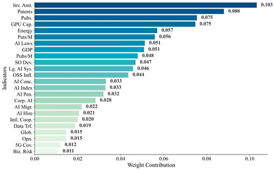
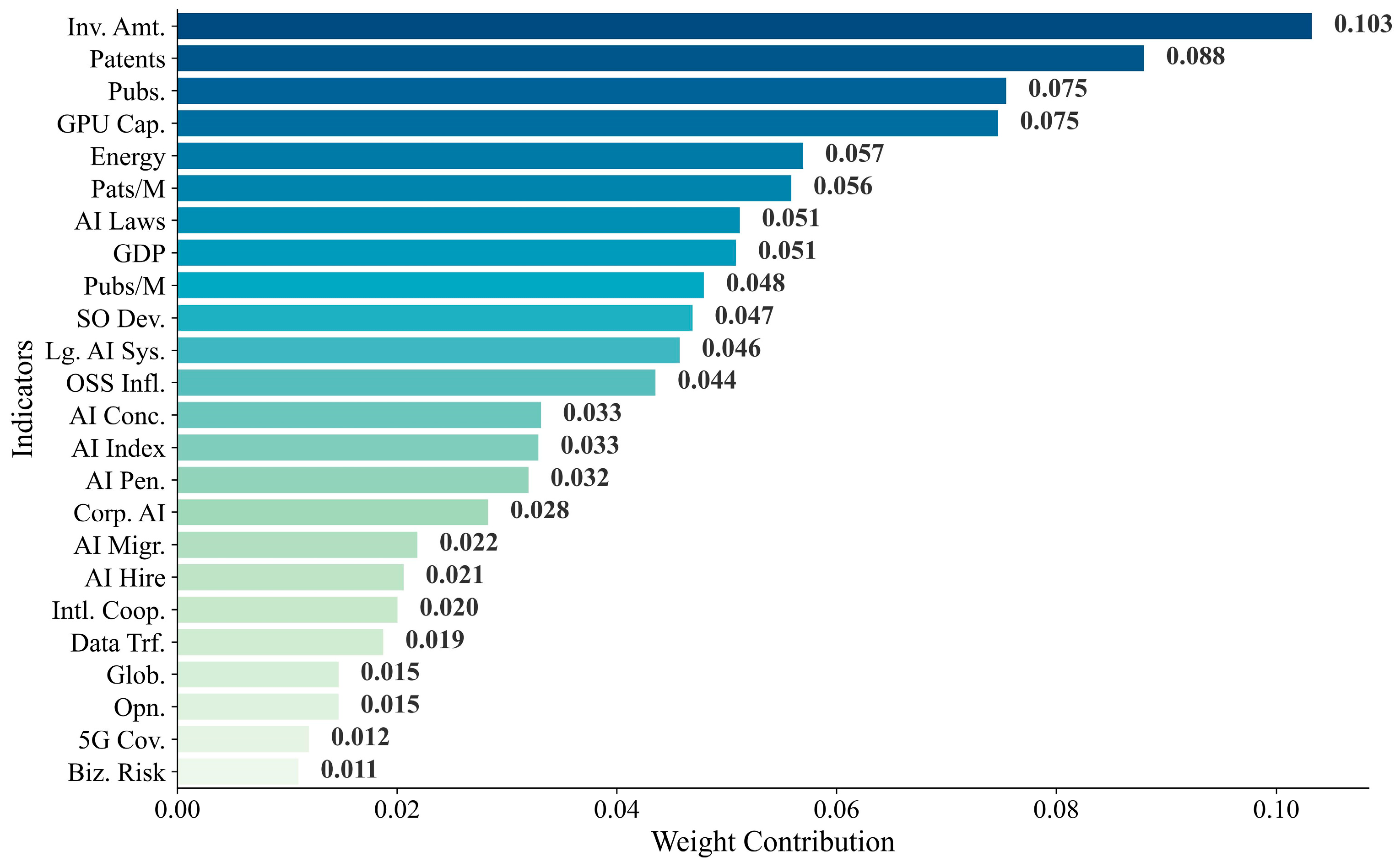
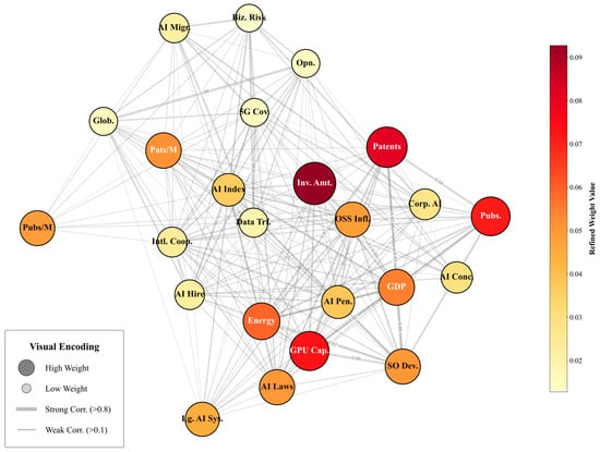
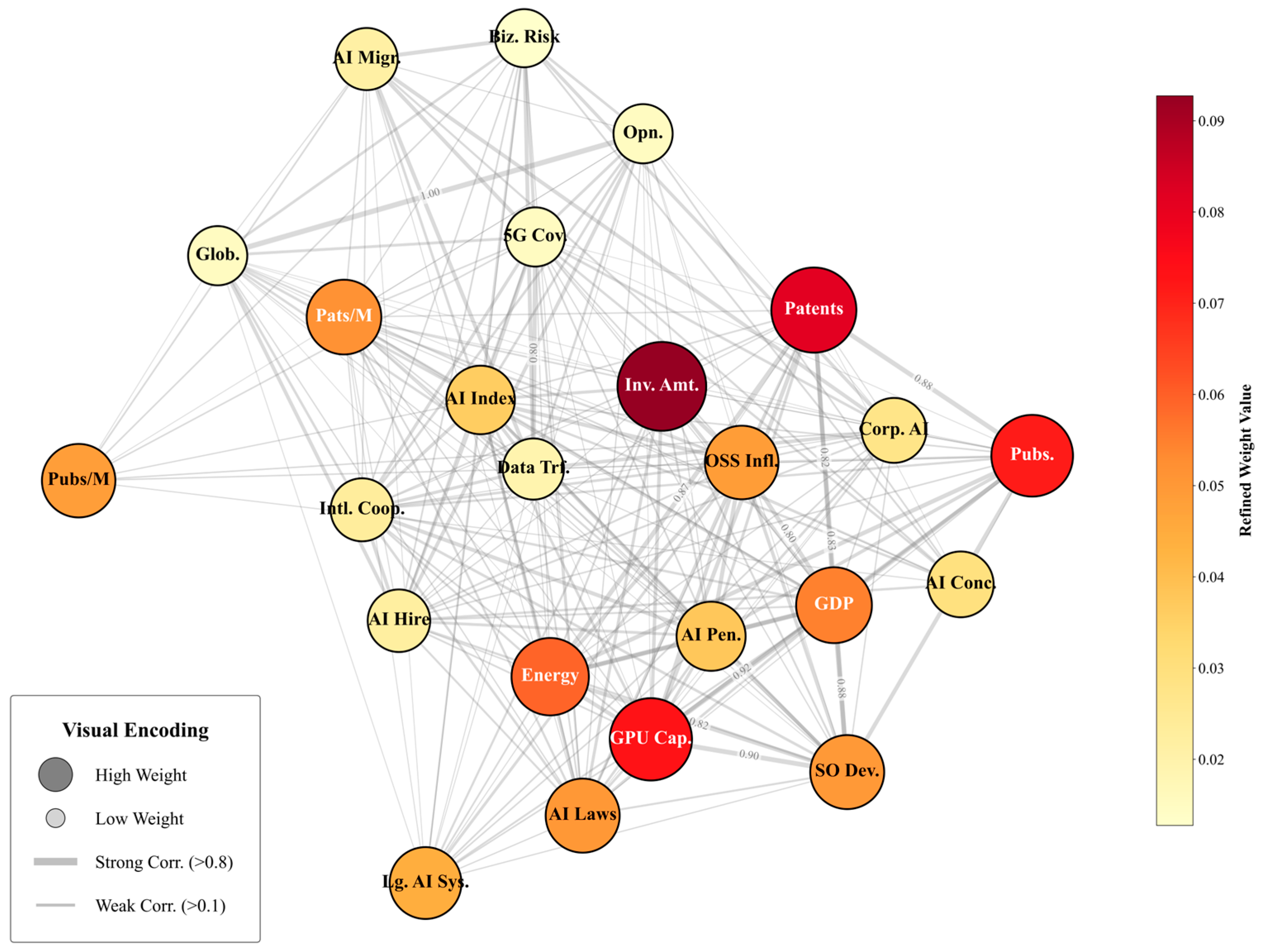
The static GNN module yields the refined weight vector ${\mathrm{w}}^{*}$, which provides an interpretable summary of indicator importance after integrating the hybrid baseline weights, the XGBoost-based sensitivity information, and the structural prior encoded by the directed indicator graph [39]. To make the refinement mechanism more explicit, define the weight change in indicator $\mathrm{j}$ as $\Delta w_j=w_j^{*}-w_j^{\left(0\right)}$, where $w_j^{\left(0\right)}$ denotes the baseline AHP–entropy weight. The learned weight distribution is shown in Figure 4.

Figure 4. Refined indicator weights learned by the static GNN module.

This change is jointly driven by three components. First, $w^{\left(0\right)}$ provides the baseline importance prior. Second, the normalized XGBoost importance vector $g$ captures nonlinear sensitivity under perturbation-response analysis. Third, the directed propagation matrix $P$ introduces structural reinforcement from upstream indicators in the learned dependency graph. Consequently, an indicator tends to receive a larger refined weight when it is important in the baseline system, exhibits strong nonlinear sensitivity, and is supported by influential directed predecessors. Overall, the most pronounced upward shifts are concentrated in structurally upstream and high-sensitivity indicators, whereas indicators with weaker nonlinear leverage or weaker upstream support exhibit smaller changes relative to the baseline weighting scheme. For example, the relatively high refined importance of Investment Amount is consistent with its upstream role in the IPOE capability-formation chain, where investment and GPU capacity affect process variables such as software development activity and talent migration, and subsequently influence output variables such as publications and patents.

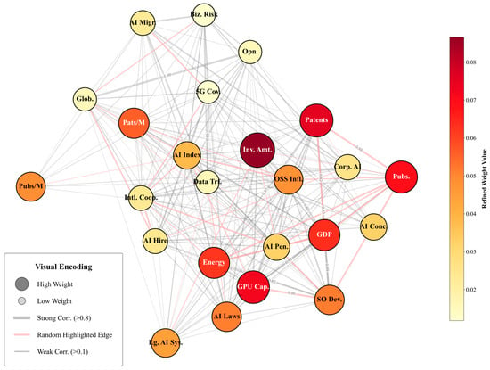
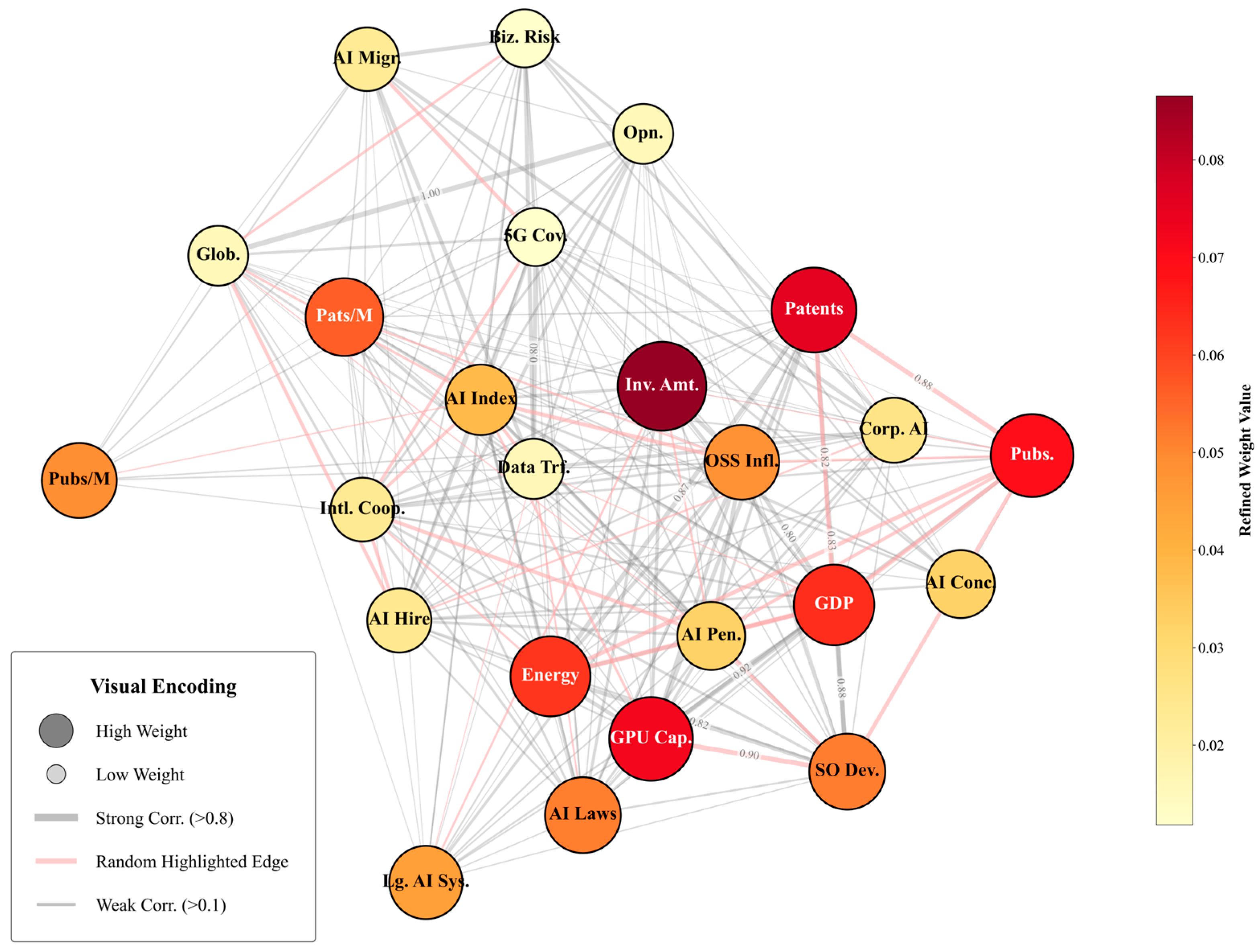
To further illustrate how these weights are embedded into the graph-based evaluation framework, Figure 5 presents the directed indicator graph with node salience overlaid on the structural prior. It should be emphasized that the GNN does not learn a new graph topology at this stage. Instead, it preserves the directed dependency structure identified in Section 3.4 and refines only the node-level importance under that structure. Accordingly, Figure 5 should be interpreted as a weighted visualization of the directed indicator graph, rather than as a newly estimated network.

Figure 5. Directed indicator graph with refined node weights overlaid on the structural prior.

4.2. Dynamic Forecasting Model for the Evolution of Competitiveness via GNN

4.2.1. ARIMA-Based Indicator Forecasting

To extend the static evaluation framework to short-term policy analysis, each standardized indicator series is forecast over 2026–2028. The forecasting inputs are taken from the standardized panel defined in Section 2.2.2, which removes scale heterogeneity while preserving the training-derived transformation. For each country–indicator pair, let ${\mathrm{x}}_{\mathrm{i},\mathrm{j},\mathrm{t}}$, $\mathrm{t}=2016,\dots ,2025$, denote the historical standardized series. The future trajectory is modeled by an ARIMA $\left(p_{i,j},d_{i,j},q_{i,j}\right)$ process:

$${\mathrm{\varphi }}_{i,\mathrm{j}}\left(L\right){(1-L)}^{d_{i,j}}{x}_{i,j,t}=c_{i,j}+{\mathrm{\theta }}_{i,\mathrm{j}}\left(L\right){\epsilon }_{i,j,t}$$

(36)

where $L$ is the lag operator, ${\mathrm{\varphi }}_{i,\mathrm{j}}\left(L\right)$ and ${\mathrm{\theta }}_{i,\mathrm{j}}\left(L\right)$ are the autoregressive and moving-average polynomials, $c_{i,j}$ is a constant term, and ${\epsilon }_{i,j,t}$ is white noise.

The orders $\left(p_{ij},d_{ij},q_{ij}\right)$ are selected using stationarity diagnostics together with an information criterion. Let ${\widehat{x}}_{i,j,t+1|t}$ denote the one-step-ahead forecast of indicator $j$ for country $\mathrm{i}$. The forecast outputs remain in the standardized space and are directly used in the subsequent dynamic GNN and optimization modules.

Given the short annual sample length, only low-order ARIMA candidates were considered, and the forecasting module is interpreted as a trend-consistent trajectory generator rather than a high-precision econometric predictor.

4.2.2. Dynamic GNN Extension

The static vector $w^{*}$ describes indicator importance over the historical window, but the relative salience of indicators may evolve over time. To account for this, a dynamic GNN module is introduced.

Define the unified indicator sequence

$${\xi }_{i,j,t}=\left\{\begin{array}{cc}{x}_{i,j,t},& t=2016,\dots , 2025,\\ {\widehat{x}}_{i,j,t},& t=2026,\dots , 2028.\end{array}\right.$$

(37)

Thus, ${\xi }_{i,j,t}$ combines the historical standardized observations and the short horizon forecasts into a unified temporal sequence that can be processed consistently by the dynamic GNN.

For each indicator $j$ and year $t$, the model next extracts two cross-country summaries, namely the annual mean level and the cross-country dispersion:

$${\overline{\xi }}_{j,t}={\displaystyle \frac{1}{N}}{\displaystyle {\displaystyle \sum }_{i=1}^N} {\xi }_{i,j,t}$$

(38)

and

$${\rho }_{j,t}={\left({\displaystyle \frac{1}{N}}{\displaystyle \sum }_{i=1}^N{\left({\xi }_{i,j,t}-{\overline{\xi }}_{j,t}\right)}^2\right)}^{1/2}.$$

(39)

The year-specific node-feature matrix is then

$$S_t=\left[\begin{array}{ccc}{\overline{\xi }}_{1,t}& {\rho }_{1,t}& w_1^{*}\\ {\overline{\xi }}_{2,t}& {\rho }_{2,t}& w_2^{*}\\ ⋮& ⋮& ⋮\\ {\overline{\xi }}_{M,t}& {\rho }_{M,t}& w_M^{*}\end{array}\right]\in {ℝ}^{M\times 3}.$$

(40)

Together with the static refined weights $w^{*}$, these two annual summaries form the year-specific node-feature matrix used by the dynamic graph module.

The same directed propagation matrix P defined in Section 4.1.1 is used in the dynamic GNN module. Based on these yearly node features, the dynamic GNN propagates information over the directed indicator graph to produce time-varying indicator weights, which are then used to compute dynamic competitiveness scores for both the historical reconstruction stage and the forecast stage. A dynamic graph convolution is defined by

$$H_t^{\left(d\right)}=\sigma \left(P{S}_t{W}_2+1b_2^{\top }\right),$$

(41)

$$u_t=\mathrm{softmax}\left(H_t^{\left(d\right)}{q}_2\right),$$

(42)

where $W_2\in {\mathrm{R}}^{3\times q_d},b_2\in {\mathrm{R}}^{q_d}, \mathrm{and} q_2\in {\mathrm{R}}^{q_d}$ are learnable parameters, and

$$u_t={(u_{1,t},\dots ,u_{M,t})}^{\top }$$

(43)

is the year-specific but common across countries weight vector, reflecting the evolving global salience of indicators over time.

For the historical window $t=2016,\dots ,2025,$ the reconstructed score is

$${\tilde{y}}_{i,t}={\displaystyle \sum }_{j=1}^M{u}_{j,t}{x}_{i,j,t}$$

(44)

The dynamic module is estimated by minimizing

$$L_{dyn}={\displaystyle \frac{1}{N{T}_h}}{\displaystyle \sum }_{t=2016}^{2025}{\displaystyle \sum }_{i=1}^N {\left({\tilde{y}}_{i,t}-y_{i,t}^{*}\right)}^2+{\mathrm{\gamma }}_1{\displaystyle \sum }_{t=2016}^{2025}\parallel u_t-w^{*}{\parallel }_2^2+{\mathrm{\gamma }}_2{\displaystyle \sum }_{t=2017}^{2025}\parallel u_t-u_{t-1}{\parallel }_2^2$$

(45)

where $y_{i,t}^{*}$ is the static GNN score defined in Section 4.1.2. The second term anchors the dynamic weights to the static structural prior, and the third term enforces temporal smoothness.

For future years $t\in \left\{2026,2027,2028\right\}$, the forecast competitiveness score of country $i$ is defined as

$${\widehat{y}}_{i,t}^{dyn}={\displaystyle \sum }_{j=1}^M{u}_{j,t}{\widehat{x}}_{i,j,t}$$

(46)

4.2.3. Uncertainty Quantification

To quantify the uncertainty of the forecast competitiveness scores, the ARIMA forecast variances are propagated through the year-specific dynamic weight vector. Here, the ARIMA module is used only to generate indicator-level forecast trajectories, whereas the dependence among indicators is mainly captured in the preceding Dynamic GNN stage through the learned directed graph structure and the year-specific common weights. Therefore, the uncertainty expression below should be interpreted as a first-order approximation rather than as a full joint uncertainty model.

Let $\mathrm{Var}\left({\widehat{x}}_{i,j,t}\right)$ denote the forecast variance returned by the ARIMA model. Assuming conditional independence of indicator forecast errors, the standard error of the forecast competitiveness score is approximated by

$$\mathrm{SE}\left({\widehat{y}}_{i,t}^{dyn}\right)={({\displaystyle \sum }_{j=1}^M{u}_{j,t}^2\mathrm{Var}({\widehat{x}}_{i,j,t}))}^{1/2}.$$

(47)

This approximation provides an uncertainty measure for the short-horizon forecast competitiveness scores and the resulting rankings over 2026–2028 under the rolling forecasting scheme, although it may still underestimate total uncertainty when forecast errors across indicators are correlated. We also note that, given that only ten annual observations are available for each country–indicator pair, introducing an additional multivariate ARIMA or factor-augmented forecasting layer would be difficult to estimate reliably in the present setting. For this reason, the current manuscript retains the above first-order approximation and leaves more elaborate joint uncertainty modeling for future work.

5. Investment Strategy Optimization via NSGA-II

5.1. Dynamic Investment-Response Mapping

The optimization problem focuses on China and considers the additional special fund allocated over a short planning horizon from 2026 to 2028. Let

$$X={\left\{x_{j,t}\right\}}_{j=1,\dots ,M; t=2026,\dots ,2028}$$

(48)

denote the investment decision matrix, where $x_{t,j}$ is the additional investment assigned to indicator j in year t, T = 3 corresponds to the years 2026–2028, and M = 24 is the number of indicators.

Let ${\widehat{x}}_{CHN,j,t}^{\left(0\right)}$ denote the baseline forecast of China’s standardized indicator $j$ in year $t$ under the no-additional-investment scenario, obtained from the rolling forecasting framework in Section 4.2. For each indicator $j$, let $c_{j,t}$ denote the marginal cost coefficient in year $t$, interpreted as the amount of capital required to increase the nonnegative rescaled indicator ${\overline{x}}_{j,t}$ by one unit. In this study, the sequence $\left\{c_{j,t}\right\}$ is estimated using the same short-horizon ARIMA procedure as in Section 4.2.1.

The direct gain induced by additional investment in the rescaled space is defined as

$${\overline{\delta }}_{j,t}={\displaystyle \frac{x_{j,t}}{c_{j,t}+ϵ}},$$

(49)

where $\mathrm{ϵ}$ is a small constant introduced for numerical stability. To ensure consistency with the standardized representation used in Section 4 and Section 5, the corresponding gain in the standardized space is defined as

$${\delta }_{j,t}={\displaystyle \frac{{\overline{\delta }}_{j,t}}{{\sigma }_j}}.$$

(50)

To reflect the persistence of policy effects, let ${\beta }_j$ denote the persistence coefficient of indicator $j$, which represents the carry-over effect of additional investment on that indicator over time. Because only ten annual observations are available for each country–indicator pair, reliable indicator-specific estimation from separate historical shock-response regressions is difficult in the present setting. Therefore, ${\beta }_j$ is treated here as a calibrated parameter in the dynamic investment-response mapping rather than as an independently estimated regression coefficient. In the main model, the persistence setting is not globally constant; instead, it is allowed to vary across indicators and years, reflecting the fact that policy effects are unlikely to decay at the same rate for all indicators or at all stages of development. The post-investment trajectory of China’s indicator $j$ is then defined recursively as

$$z_{\mathrm{CHN},j,t}={\widehat{x}}_{\mathrm{CHN},j,t}^{\left(0\right)}+{\delta }_{j,t}+{\beta }_j\left(z_{\mathrm{CHN},j,t-1}-{\widehat{x}}_{\mathrm{CHN},j,t-1}^{\left(0\right)}\right).$$

(51)

The total additional budget is fixed as $\mathrm{B}=5\times {10}^{11}$ RMB as a policy simulation scenario.

5.2. Bi-Objective Optimization Model for Investment Strategy

The investment strategy is evaluated in a closed loop through the dynamic GNN developed in Section 4.2. In this way, each candidate allocation plan is fed back into the same standardized forecasting-and-scoring framework, so that the investment strategy is evaluated under the same dynamic mechanism used for competitiveness prediction. For year t, define the updated country-level indicator panel under strategy X as

$${\tilde{\xi }}_{i,j,t}\left(X\right)=\left\{\begin{array}{cc}{z}_{j,t}\left(X\right),& i=\mathrm{CN},\\ {\widehat{x}}_{i,j,t},& i\ne \mathrm{CN}\end{array}\right.$$

(52)

where ${\widehat{x}}_{i,j,t}$ denotes the baseline forecast for country $i\ne \mathrm{CN}$.

Replacing the baseline future panel by ${\tilde{\xi }}_{i,j,t}\left(X\right)$, the year-specific node-feature matrix in Section 4.2.2 is updated accordingly, and the trained dynamic GNN yields the corresponding year-specific weight vector

$$u_t\left(X\right)={\left(u_{1,t}\left(X\right),\dots ,u_{M,t}\left(X\right)\right)}^{\mathrm{T}}.$$

(53)

China’s dynamic competitiveness score under strategy X is then defined as

$$Y_t^{CN}\left(X\right)={\displaystyle \sum }_{j=1}^M{u}_{j,t}\left(X\right)z_{j,t}\left(X\right).$$

(54)

The primary objective is to maximize China’s AI competitiveness at the end of the short planning horizon, i.e., in 2028:

$$f_1\left(X\right)=Y_{2028}^{\mathrm{CN}}\left(X\right).$$

(55)

To avoid excessively abrupt policy shifts, an intertemporal smoothness objective is introduced:

$$f_2\left(X\right)={{\displaystyle \sum }}_{t=2027}^{2028}\parallel x_t-x_{t-1}{\parallel }_2^2,$$

(56)

where $x_t={(x_{t,1},x_{t,2},\dots ,x_{t,M})}^{\mathrm{T}}.$

Accordingly, the resulting bi-objective optimization problem can be formulated as

$$max{f}_1\left(X\right)=Y_{2028}^{CN}\left(X\right),$$

(57)

$$min{f}_2\left(X\right)={\sum }_{t=2027}^{2028}\parallel x_t-x_{t-1}{\parallel }_2^2,$$

(58)

$$s.t.{\displaystyle \sum }_{t=2026}^{2028}{\displaystyle \sum }_{j=1}^M x_{t,j}=B,$$

(59)

$$x_{t,j}\ge 0,t=2026,\dots ,2028,j=1,\dots ,M,$$

(60)

$$0\le {\mu }_j+{\sigma }_j{z}_{CHN,j,t}\left(X\right)\le 100,\hspace{1em}j=1,\dots ,M,t=2026,2027,2028.$$

(61)

The last constraint ensures that the post-investment trajectory, when mapped back to the nonnegative rescaled space, remains within the admissible range [0, 100]. The first objective directly corresponds to the policy target of maximizing China’s terminal AI competitiveness over a statistically more reliable short horizon, while the second objective ensures that the recommended strategy remains implementable and stable across consecutive years.

5.3. Solution Strategy Based on NSGA-II

5.3.1. Design of NSGA-II Algorithm

The above bi-objective problem is solved by the NSGA-II algorithm. Each candidate solution is encoded as a real-valued chromosome corresponding to the matrix

$$X=\left[x_{t,j}\right]\in {\mathrm{R}}_{+}^{3\times 24}.$$

(62)

Equivalently, each chromosome has length $T\times M=72.$ This encoding allows each chromosome to represent a complete year-by-year, indicator-by-indicator allocation strategy, which can then be evaluated by the dynamic response mapping and the dynamic GNN module.

The initialization step generates a population of nonnegative investment plans that satisfy the total-budget constraint. Each chromosome is then decoded into the annual investment matrix X, from which the post-investment indicator path $z_{j,t}$ is computed through the dynamic response mapping in Section 5.1. The updated country panel ${\tilde{\xi }}_{i,j,t}\left(X\right)$ is next passed into the dynamic GNN evaluation module, yielding the terminal competitiveness objective $f_1\left(X\right)$. The policy-volatility objective $f_2\left(X\right)$ is computed simultaneously from the temporal allocation sequence.

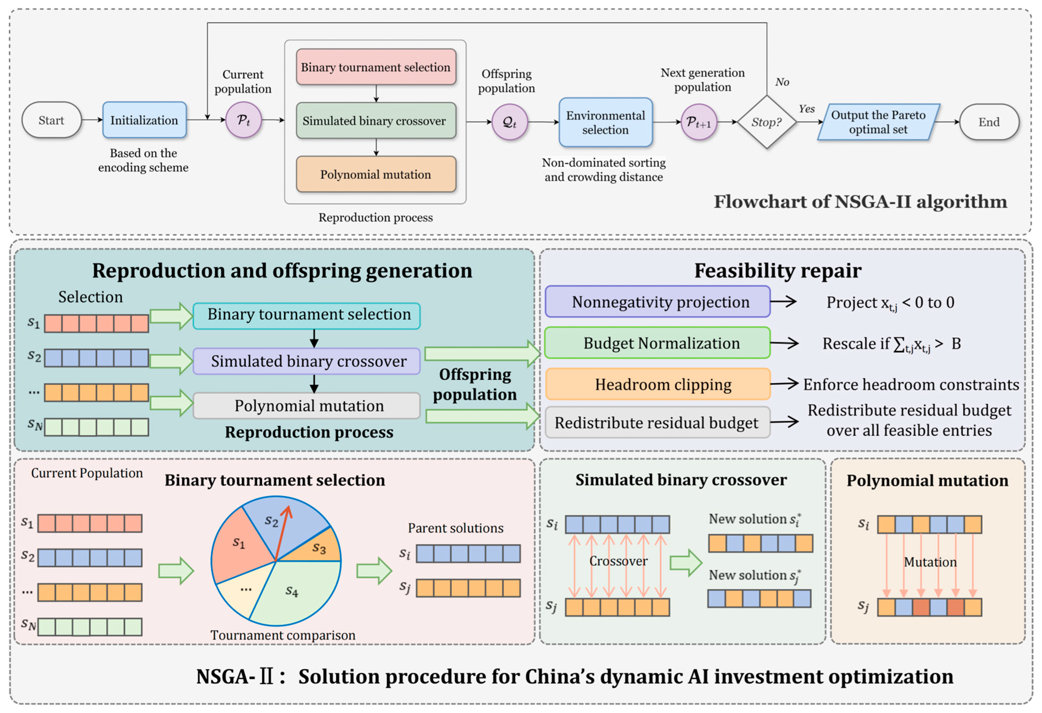
NSGA-II then performs fast non-dominated sorting and crowding-distance calculation to preserve both convergence and diversity on the Pareto front. Simulated binary crossover and polynomial mutation are adopted as the variation operators. After crossover and mutation, each offspring is repaired to satisfy the feasibility conditions by enforcing nonnegativity, budget normalization, and capacity clipping.

The optimization terminates after a prescribed number of generations or when the Pareto front stabilizes. The output is a set of non-dominated investment strategies that characterize the trade-off between long-term competitiveness and policy stability. The overall workflow of the proposed NSGA-II solution procedure is illustrated in Figure 6, and the detailed pseudo-code is provided in Algorithm 1.

Figure 6. Overall Framework of The Proposed NSGA-II Algorithm.

Algorithm 1. NSGA-II for the bi-objective investment optimization problem

$$\begin{gathered} \mathbf{Input}\mathbf{:} \mathrm{Population} \mathrm{size} N_{pop}, \mathrm{maximum} \mathrm{number} \mathrm{of} \mathrm{generations} G_{max}, \mathrm{total} \mathrm{budget} B, \mathrm{baseline} \mathrm{forecasts} {\widehat{x}}^{\left(0\right)}\left(j,t\right), \mathrm{marginal} \cos \mathrm{t} \mathrm{coefficients} c_{\left(j,t\right)}, \mathrm{persistence} \mathrm{coefficients} {\beta }_j, \mathrm{trained}\mathrm{dynamic}\mathrm{GNN}\mathrm{evaluation}\mathrm{model}; \\ \mathbf{Output}\mathbf{:}\mathrm{Feasible}\mathrm{Pareto}\mathrm{optimal}\mathrm{set}\mathrm{NDSet}; \\ \mathbf{1} P_0 \leftarrow \mathrm{Generate\; the\; initial\; feasible\; population\; based\; on\; the\; encoding\; scheme} \\ \hspace{1em}\hspace{1em}\hspace{1em}\hspace{1em} \mathrm{and\; the\; total\; budget\; constraint}; \\ \mathbf{2} \mathbf{for}g=1,2,\dots ,G_{max} \mathrm{do} \\ \mathbf{3}\hspace{1em}\hspace{1em}\hspace{1em}{Q}_g\leftarrow \varnothing ; \\ \mathbf{4}\hspace{1em}\hspace{1em}\hspace{1em}\mathbf{for}i=1,2,\hspace{0.17em},\mathrm{N}\mathrm{do} \\ \mathbf{5} \hspace{1em}\hspace{1em}\hspace{1em}\hspace{1em}\mathrm{Selection} \leftarrow \mathrm{Randomly} \mathrm{select} \mathrm{two} \mathrm{solutions} \mathrm{from} P_{\left(g-1\right)} \\ \hspace{1em}\hspace{1em}\hspace{1em}\hspace{1em}\hspace{1em}\hspace{1em}\hspace{1em}\hspace{1em}\hspace{1em} \mathrm{using\; binary\; tournament\; selection}; \\ \mathbf{6} \hspace{1em}\hspace{1em}\hspace{1em}\hspace{1em}\mathrm{Crossover} q \leftarrow \mathrm{Perform} \mathrm{simulated} \mathrm{binary} \mathrm{crossover} \mathrm{on} p_1 and p_2 \\ \hspace{1em}\hspace{1em}\hspace{1em}\hspace{1em}\hspace{1em}\hspace{1em}\hspace{1em}\hspace{1em}\hspace{1em}\hspace{1em} \mathrm{under\; crossover\; probability}; \\ \mathbf{7} \hspace{1em}\hspace{1em}\hspace{1em}\hspace{1em}\mathrm{Mutation}\mathrm{q}\leftarrow \mathrm{Perform\; polynomial\; mutation\; on\; q\; under\; mutation\; probability}; \\ \mathbf{8} \hspace{1em}\hspace{1em}\hspace{1em}\mathrm{X}=\left[x_{\left(t,j\right)}\right]\leftarrow \mathrm{Decode\; q\; into\; the\; annual\; investment\; matrix}; \\ \mathbf{9} \hspace{1em}\hspace{1em}\hspace{1em}\mathrm{Repair\; X\; for\; feasibility}: \\ \mathbf{10} \hspace{1em}\hspace{1em}\hspace{1em}\hspace{1em} \mathrm{Project\; all\; negative\; entries\; of\; X\; to\; zero}; \\ \mathbf{11} \hspace{1em}\hspace{1em}\hspace{1em}\hspace{1em} \mathbf{if} {\displaystyle \sum _{\left(t,j\right)}}{x}_{\left(t,j\right)}>\mathrm{B\; then} \\ \mathbf{12} \hspace{1em}\hspace{1em}\hspace{1em}\hspace{1em} \hspace{1em}\hspace{1em}{x}_{\left(t,j\right)} \leftarrow \left({\displaystyle \frac{B}{{\sum }_{\left(t,j\right)}{x}_{\left(t,j\right)}}}\right)x_{\left(t,j\right)}; \\ \mathbf{13} \hspace{1em}\hspace{1em}\hspace{1em}\hspace{1em} \mathbf{end\; if} \\ \mathbf{14} \hspace{1em}\hspace{1em}\hspace{1em}\hspace{1em} \mathrm{Clip\; the\; violating\; entries\; to\; satisfy\; the\; cumulative\; headroom\; constraints}; \\ \mathbf{15} \hspace{1em}\hspace{1em}\hspace{1em}\hspace{1em} \mathbf{if}\mathrm{unused\; budget\; remains\; after\; clipping\; then} \\ \mathbf{16} \hspace{1em}\hspace{1em}\hspace{1em}\hspace{1em}\hspace{1em}\hspace{1em}\mathrm{Redistribute\; the\; residual\; budget\; over\; the\; remaining\; feasible\; entries\; and\; update\; X\; until\; feasibility\; is\; restored} \\ \mathbf{17} \hspace{1em}\hspace{1em}\hspace{1em}\hspace{1em} \mathbf{end\; if} \\ \mathbf{18} \hspace{1em}\hspace{1em}\hspace{1em} \mathrm{q}\leftarrow \mathrm{Encode\; the\; repaired\; investment\; matrix\; X\; into\; chromosome\; form}; \\ \mathbf{19}\hspace{1em}\hspace{1em}\hspace{1em}{\Delta }_{\left(j,t\right)} \leftarrow \left({\displaystyle \frac{x_{\left(t,j\right)}}{c_{\left(j,t\right)}+\epsilon }}\right), \mathrm{and} \mathrm{construct} z_{\left(j,t\right)}\left(X\right); \\ \mathbf{20}\hspace{1em}\hspace{1em}\hspace{1em}{\xi }_{\left(i,j,t\right)}\left(X\right)\leftarrow \mathrm{Form\; the\; updated\; country-level\; indicator\; panel}; \\ \mathbf{21}\hspace{1em}\hspace{1em}\hspace{1em}{f}_1\left(q\right) \leftarrow Y_{2028}^{CN}\left(q\right); \\ \mathbf{22}\hspace{1em}\hspace{1em}\hspace{1em}{f}_2\left(q\right) \leftarrow {{\displaystyle \sum }}_{t=2027}^{2028}\parallel x_t-x_{t-1}{\parallel }_2^2; \\ \mathbf{23}\hspace{1em}\hspace{1em}\hspace{1em}{Q}_g \leftarrow Q_g\cup \left\{q\right\},\mathrm{evaluate\; and\; record\; the\; offspring\; solution\; q}; \\ \mathbf{24}\hspace{1em}\hspace{1em}\mathbf{end\; for} \\ \mathbf{25}\hspace{1em}\hspace{1em}{P}_g\leftarrow \mathrm{Perform\; non-dominated\; sorting\; and\; crowding-distance-based} \\ \mathrm{environmental} \mathrm{selection} \mathrm{on} P_{\left(g-1\right)}\cup Q_g; \\ \mathbf{26}\hspace{1em}\mathbf{end\; for} \\ \mathbf{27}\hspace{1em}\mathrm{NDSet} \leftarrow \mathrm{Perform} \mathrm{non-dominated} \mathrm{sorting} \mathrm{on} \mathrm{the} \mathrm{final} \mathrm{population} P_{G_{max}}, \\ \hspace{1em}\hspace{1em}\hspace{1em}\hspace{1em} \mathrm{and\; obtain\; the\; feasible\; Pareto\; optimal\; set;} \\ \mathbf{28}\hspace{1em}\mathbf{return}\mathrm{NDSet} \end{gathered}$$

5.3.2. Pareto Set Generation and Representative Solution Extraction

Let $P$ denote the Pareto-optimal solution set returned by NSGA-II. To facilitate interpretation and policy recommendation, three representative solutions are extracted from $P$.

The maximum-score strategy is defined as

$$X^{\mathrm{score}}=\arg \underset{X\in P}{\max }{f}_1\left(X\right),$$

(63)

which emphasizes terminal competitiveness.

The minimum-variance strategy is defined as

$$X^{\mathrm{var}}=\arg \underset{X\in P}{\min }{f}_2\left(X\right),$$

(64)

which emphasizes policy smoothness and stability.

To identify a balanced compromise solution, both objectives are first normalized:

$${\tilde{f}}_1\left(X\right)={\displaystyle \frac{f_1\left(X\right)-f_1^{min}}{f_1^{max}-f_1^{min}}},$$

(65)

$${\tilde{f}}_2\left(X\right)={\displaystyle \frac{f_2^{max}-f_2\left(X\right)}{f_2^{max}-f_2^{min}}},$$

(66)

where $f_1^{\min },f_1^{\max },f_2^{\min },f_2^{\max }$ are computed over the Pareto set $P$. The balanced strategy is then chosen as the Pareto point closest to the ideal point (1,1):

$$X^{†}=\arg \underset{X\in P}{\min }\sqrt{{(1-{\tilde{f}}_1\left(X\right))}^2+{(1-{\tilde{f}}_2\left(X\right))}^2}.$$

(67)

This rule avoids the use of arbitrary scalarization weights and provides a transparent compromise between competitiveness enhancement and policy stability. The selected strategy yields both a year-by-year investment schedule and an indicator-by-indicator allocation profile, which are reported in Section 6.

6. Experiments and Results

6.1. Validation of the Graph-Based Evaluation Framework

Before presenting the forecasting and optimization results, the graph-based evaluation framework is first validated. Since the dependency graph learned in Section 3.4 is used as the structural prior for the static GNN refinement in Section 4.1, this part examines the stability of the learned topology, the effect of alternative graph settings, and the robustness of the refinement module.

The stability of the learned dependency graph is evaluated by repeated subsampling. The Bayesian network structure is relearned under the same IPOE prior, and the retention frequency of each directed edge is then computed. Figure 7 reports the resulting bootstrap stability of the learned graph. The edge labels give the corresponding retention frequencies, and the highlighted edges indicate the dependencies that remain stable across repeated subsampling.

Figure 7. Bootstrap stability of the learned dependency graph with refined node weights.

The downstream validity of the learned graph is further examined under alternative graph settings, including an alternative-score graph, an expert-prior graph, a no-graph baseline, and a null graph with preserved degree sequence. Table 3 summarizes the corresponding results. The proposed graph gives the best performance under the same evaluation framework, which shows that the learned dependency structure contributes to the downstream task beyond a purely descriptive topology.

Table 3. Structural robustness and comparative validation of the learned dependency graph.

Graph Setting	Score Criterion/Source	RMSE	R2
Proposed model	AIC-based Bayesian network	0.006562	0.999998
Alternative-score graph	BIC-based Bayesian network	0.0073	0.999997
Expert-prior graph	IPOE/domain prior only	0.0087	0.999995
No-graph baseline	Identity adjacency	0.0099	0.999993
Null graph	Random graph with preserved degree sequence	0.0148	0.999986

Note: The shaded row highlights the proposed model, which achieves the best overall performance among the compared methods in terms of RMSE and R².

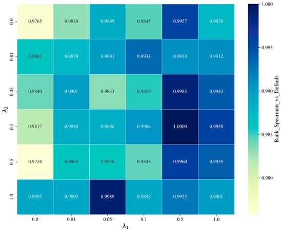
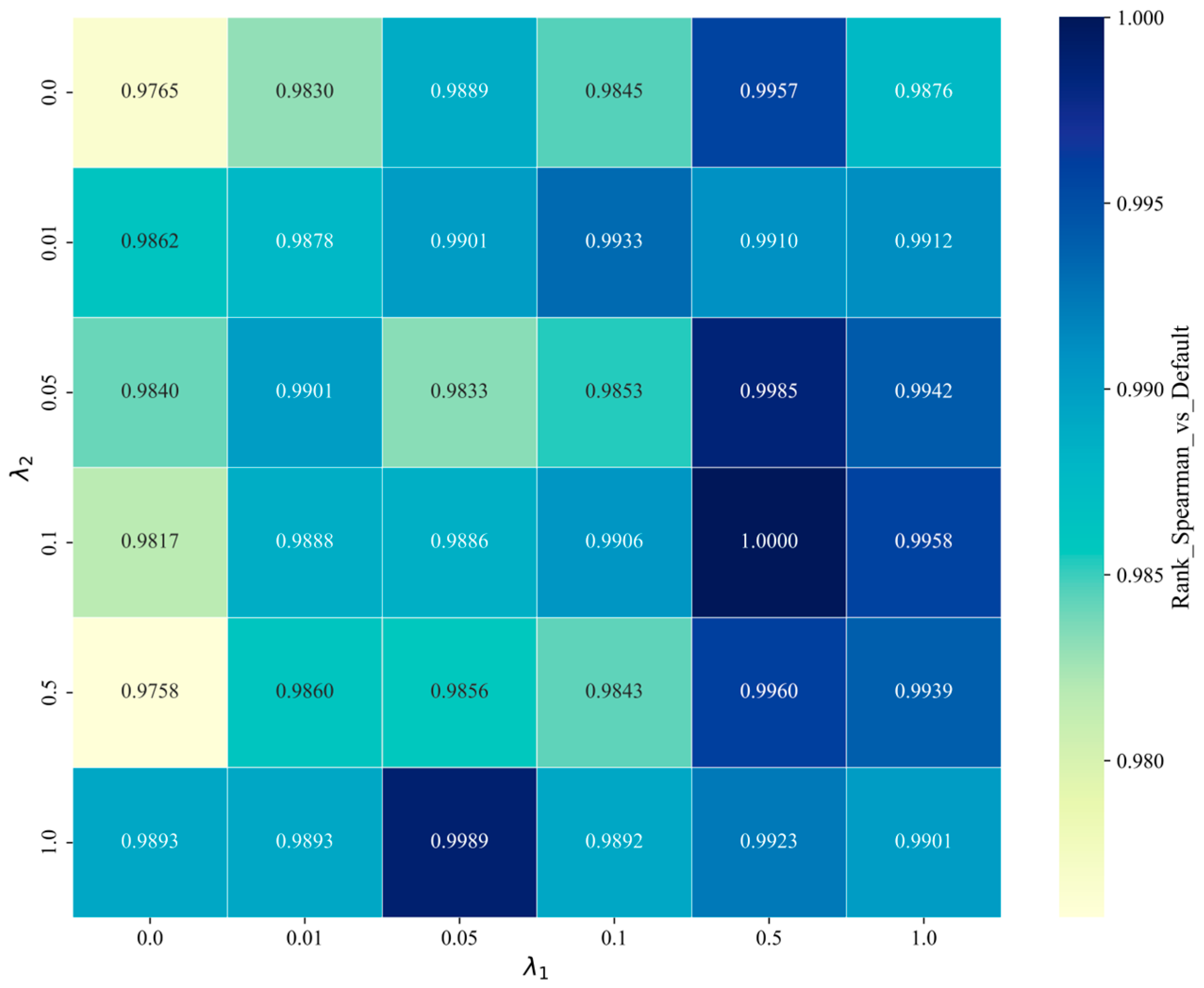
The role of graph-based refinement is further examined by comparing the full GNN with a ridge baseline and an identity-adjacency baseline. In the identity-adjacency case, the graph structure is replaced by the identity matrix, so that no inter-indicator topology is used in refinement. Table 4 reports the resulting ranking consistency. In addition, Figure 8 shows the sensitivity of the final 2025 ranking to λ1 and λ2. The ranking remains unchanged over the tested parameter grid, indicating that the refinement result is stable with respect to the regularization settings.

Table 4. Baseline comparison for the graph-refinement module.

Baseline Setting	Ranking Consistency
Full GNN (The Proposed Model)	1.000
Identity Adjacency	0.867
Ridge Baseline	0.733

Figure 8. Sensitivity of the final 2025 ranking under different λ₁ and λ₂ settings.

Beyond the internal structural and module-level baselines above, it is also useful to position the proposed framework against representative existing evaluation routes. Compared with representative existing routes, most conventional approaches remain either static and linear or insufficiently expressive in terms of structural dependency modeling, whereas the proposed framework integrates dependency learning, graph-based refinement, short-horizon forecasting, and policy-oriented allocation in a unified pipeline. To this end, Table 5 Comparative results against representative existing methods and implemented baselines. reports a broader comparison with a classical AHP–Entropy with TOPSIS baseline and a machine learning weighting baseline, together with the implemented graph-related baselines under the same evaluation target. This comparison provides a more direct reference for assessing the relative advantage of the proposed causality-guided graph framework.

Table 5. Comparative results against representative existing methods and implemented baselines.

Method	RMSE	R2
Proposed model	0.006562	0.999998
Machine learning weighting baseline	0.0091	0.999994
Alternative-score graph	0.0073	0.999997
Expert-prior graph	0.0087	0.999995
No-graph baseline	0.0099	0.999993
Null graph	0.0148	0.999986
AHP–Entropy with TOPSIS baseline	0.0118	0.999991

As shown in Table 5, the proposed model achieves the best overall fit among the compared methods, indicating that the explicit integration of directed dependency learning and graph-based refinement improves evaluation performance beyond both classical weighted ranking routes and non-graph data-driven weighting baselines.

6.2. Importance Stability and Competitiveness Forecasting

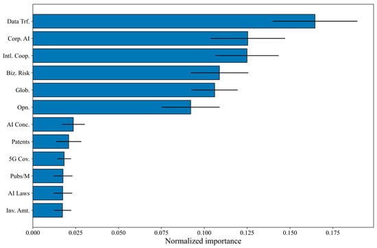
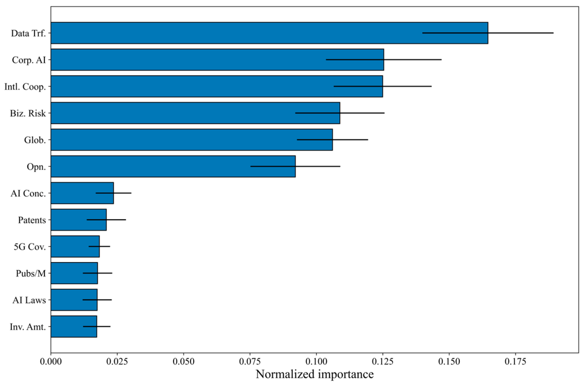
The stability of the perturbation-based importance analysis is first examined through a country-level bootstrap procedure. Since the XGBoost importance scores are used as the sensitivity signal in the graph-refinement stage, it is necessary to assess whether the resulting importance pattern is reproducible beyond a single historical panel. To this end, countries are resampled with replacement across repeated bootstrap runs, and the perturbation dataset and XGBoost model are reconstructed in each replicate. Figure 9 (Variations in global AI competitiveness across countries over the past and future decades) reports the mean importance scores together with their dispersion across bootstrap runs. The results show that the most influential indicators remain concentrated in a relatively stable subset, although several middle-ranked indicators still exhibit noticeable variation across bootstrap replicates.

Figure 9. Bootstrap stability of perturbation-based XGBoost importance scores across country-level resamples.

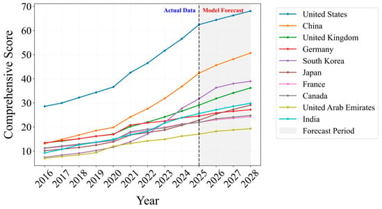
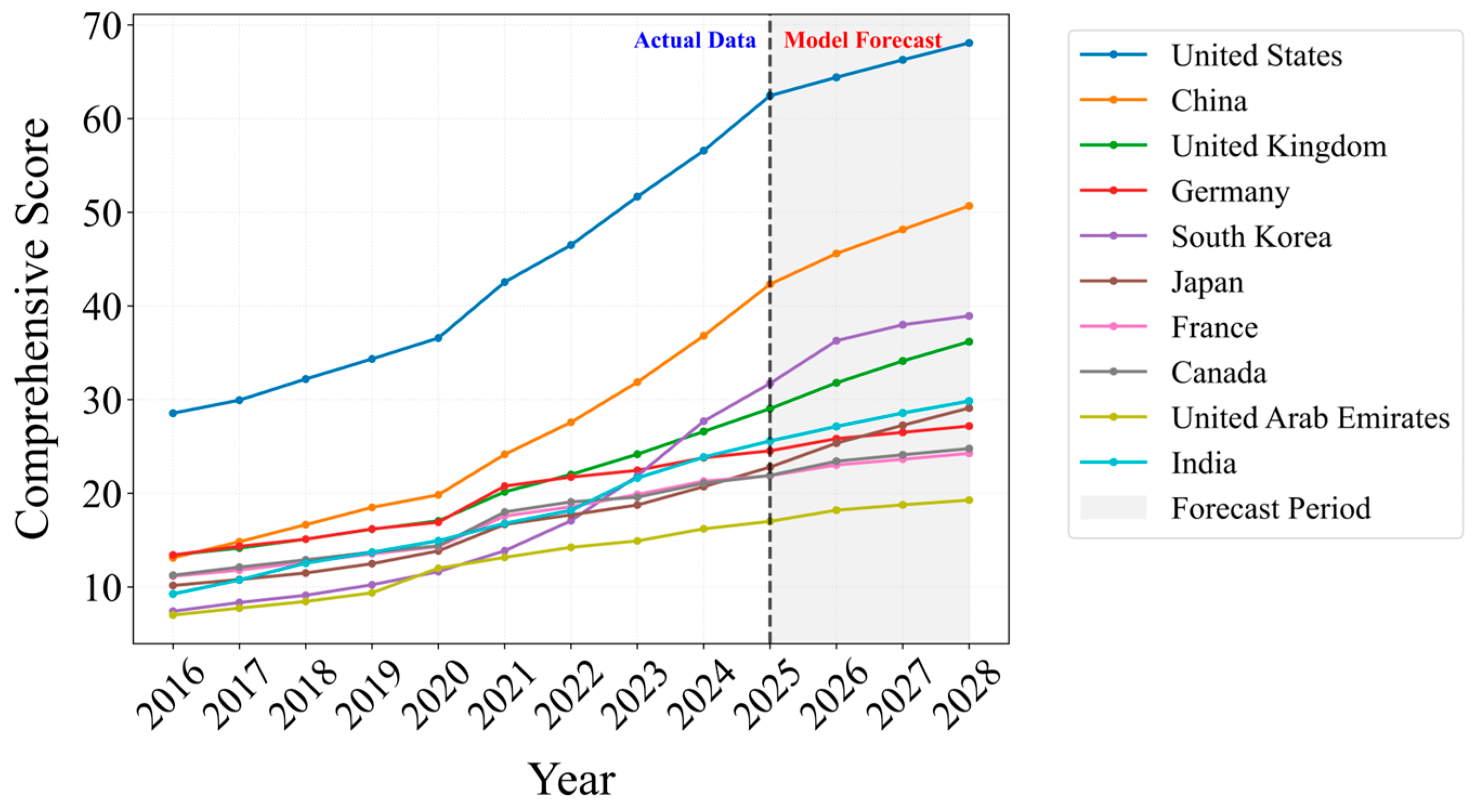
On this basis, the short-horizon forecasting results of national AI competitiveness are reported. As illustrated in Figure 10, the overall scores of the selected countries show a clear upward trend from 2016 to 2028. The United States and China remain the top two economies throughout the period, with the United States preserving a clear lead and China continuing to narrow the gap through sustained growth. Over the forecast period of 2025–2028, the United Kingdom and South Korea exhibit relatively strong growth and remain in the third and fourth positions, respectively. India also shows a notable upward trend and further strengthens its position relative to several traditional developed economies. By contrast, Canada and the United Arab Emirates maintain comparatively modest growth and remain in the lower part of the ranking. Overall, the forecast results suggest that the leading positions remain stable in the short run, while the middle-tier economies continue to undergo visible reordering.

Figure 10. Variations in global AI competitiveness across countries over the past and future decades.

6.3. Investment Optimization Results

Based on the forecasted competitiveness trajectories, the policy-oriented investment optimization results are further examined for China. This part reports the forecasted cost-side inputs, the Pareto trade-off between competitiveness enhancement and policy stability, the selected representative strategy, and the corresponding allocation profile and post-investment competitiveness trajectory. The aim is to show how the proposed framework converts structural evaluation and dynamic forecasting into an implementable investment recommendation.

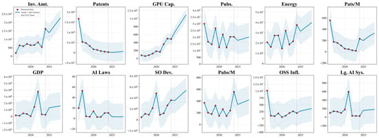
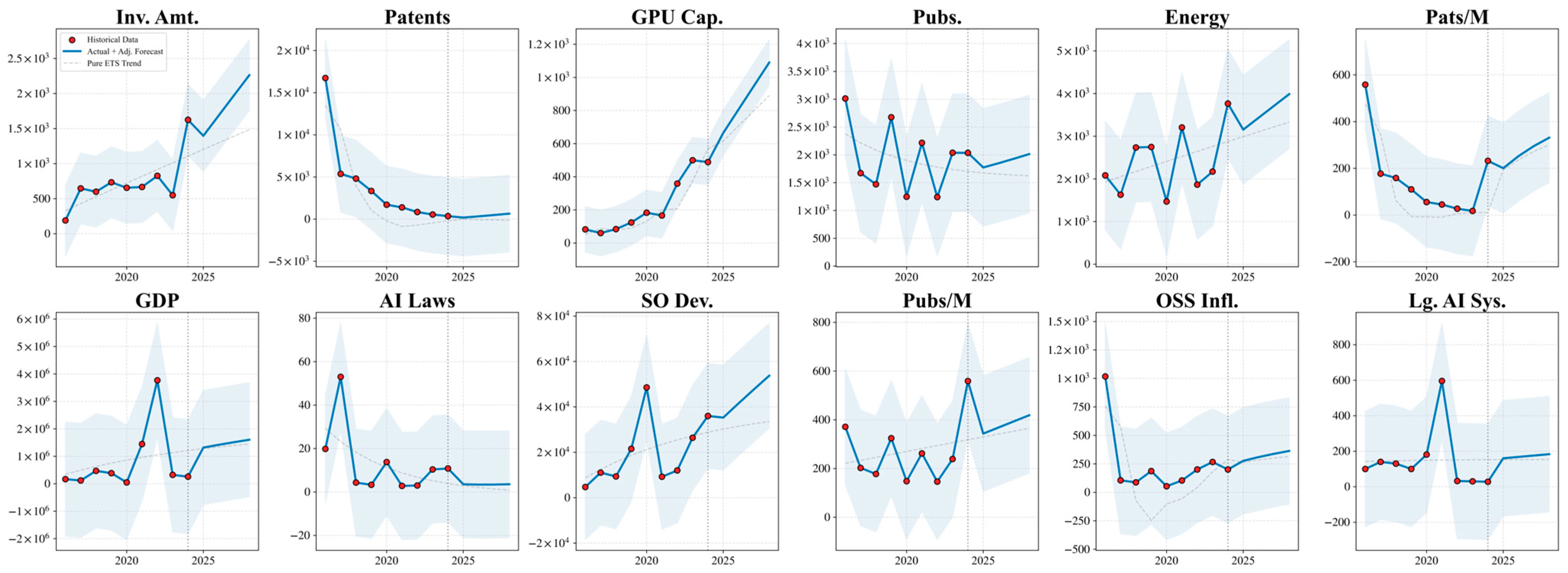
To characterize the cost-side inputs required by the investment optimization module, we further forecast the marginal cost coefficients associated with China’s key indicators over the short planning horizon 2026–2028, using historical data from 2016 to 2025. For readability, Figure 11 reports the historical and forecast trajectories of the top 12 weighted indicators. The vertical axis represents the estimated cost required to increase the corresponding indicator by one unit. Overall, the projected cost paths suggest substantial heterogeneity across indicators rather than a uniform trend. In particular, indicators such as Investment Amount, GPU Capabilities, and Software Development Activity exhibit relatively pronounced upward trajectories, implying that further improvement in these domains may require increasingly intensive resource input. By contrast, several regulatory and per capita indicators remain comparatively stable over the short horizon. These projected marginal-cost patterns provide the cost-side inputs for the subsequent investment optimization analysis.

Figure 11. Historical and short-horizon forecast trajectories of China’s marginal cost indicators for the top 12 weighted indicators (2016–2028).

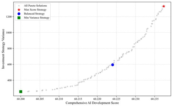
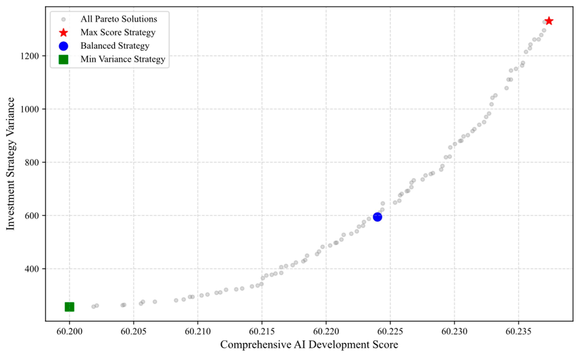
To provide a more precise interpretation of the optimal investment scheme, this section presents the Pareto frontier obtained by applying the NSGA-II algorithm to optimize cross-sectoral investment allocation under a fixed total budget of RMB 500 billion. The resulting solution set reveals the trade-off between the overall AI development score and the continuity of the investment strategy, as illustrated in Figure 12 and Table 6. The Min Variance strategy emphasizes balanced allocation, offering high policy stability but limited potential for breakthrough innovation. In contrast, the maximum-score strategy concentrates resources in a few key domains, which slightly improves the overall competitiveness score but leads to a substantial increase in investment variance. Given that the differences in AI development scores among the Pareto solutions are relatively small, while the variance varies significantly across strategies, prioritizing stability becomes a more practical choice. Therefore, this study adopts the minimum-variance strategy located at the lower-left end of the Pareto frontier. This strategy maintains an AI competitiveness score comparable to other solutions while significantly reducing allocation variability, thereby ensuring higher policy stability and implementation feasibility. As a result, it provides a more robust structural basis for the proposed investment plan.

Figure 12. Pareto front under 500 billion RMB investment.

Table 6. Numerical Characteristics.

Strategy	Comprehensive Score	$\mathbf{Annual} \mathbf{Variance}$ (σ2)
Min Variance	60.20	2.5 × 102
Balanced	60.22	6.0 × 102
Max Score	60.24	1.3 × 103

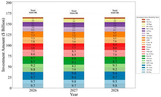
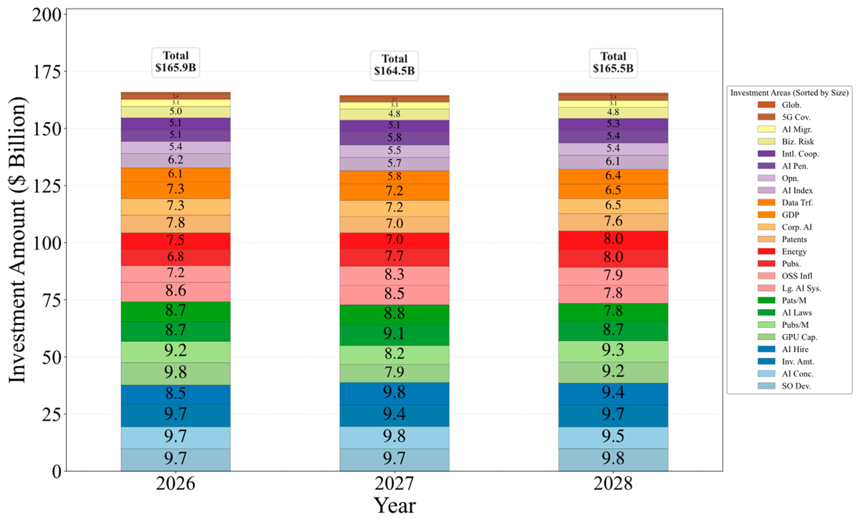
Figure 13 illustrates the detailed investment allocation scheme corresponding to the minimum-variance strategy optimized by the NSGA II algorithm under a total investment scale of RMB 500 billion. Within this allocation structure, investment amount, software development and GDP for the largest proportions, each receiving annual investments ranging from RMB 8 billion to RMB 10 billion, thereby constituting the core pillars for enhancing AI competitiveness. Meanwhile, key indicators including large scale model systems, AI related academic publications, and 5G coverage are also supported by sustained and stable funding. This multi-domain coordinated investment framework achieves near optimal overall performance while effectively controlling allocation variance and preventing excessive resource concentration. It translates the abstract Pareto optimal solution into an actionable policy blueprint and provides decision makers with a concrete and implementable investment pathway.

Figure 13. Investment plan under 500 billion RMB investment with Min-Variance Strategy.

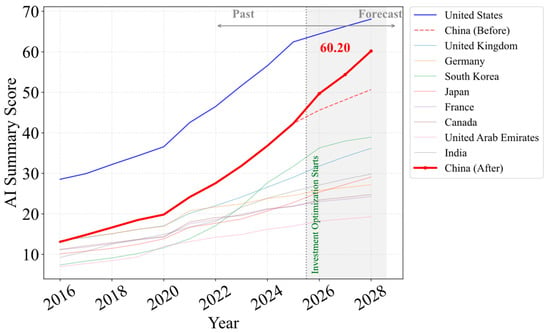
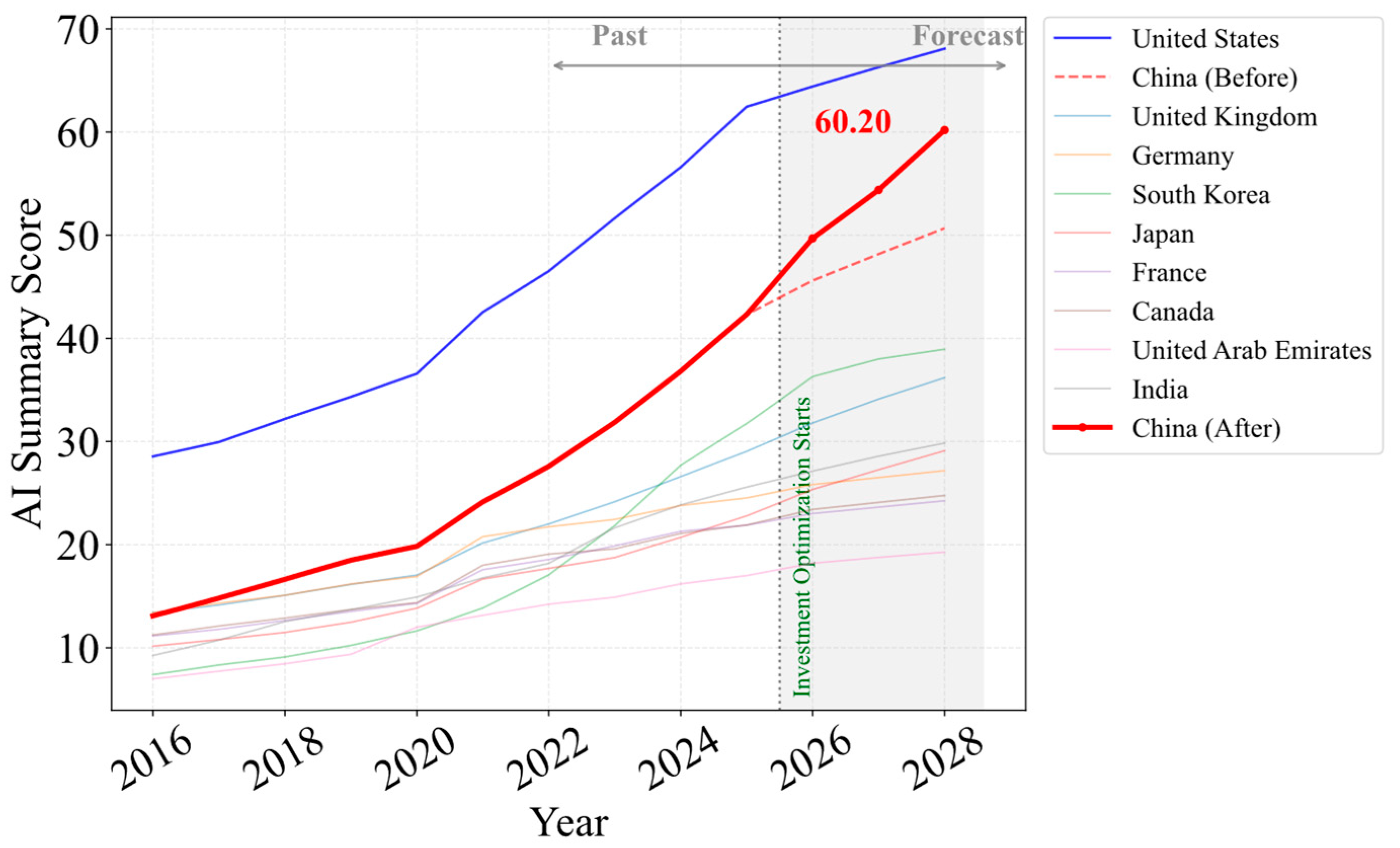
Using the optimal RMB 500 billion investment strategy identified by the NSGA-II multi-objective optimization framework, we further project the evolution of China’s AI competitiveness over the subsequent forecast horizon, as shown in Figure 14. Following the implementation of the optimized investment scheme, China’s projected trajectory (“China After”) rises distinctly above the baseline path (“China Before”), indicating that the proposed allocation strategy can effectively enhance the growth momentum of national AI competitiveness. More importantly, the results show that the gap between China and the United States is substantially reduced after the investment intervention. Whereas a clear competitiveness disparity exists at the beginning of the forecast period, the optimized trajectory enables China to shift from an initially lagging position to a sustained catching-up trend, thereby progressively narrowing the distance to the global leader. By the end of the projection horizon, China’s AI summary score reaches 60.20 under the optimized strategy, demonstrating that large-scale strategic investment, when allocated through the proposed optimization framework, can produce a pronounced marginal improvement in national AI capability. Overall, these findings suggest that the RMB 500 billion investment scheme not only raises China’s absolute competitiveness level, but also accelerates its convergence toward the technological frontier, thereby reshaping the near-term pattern of global AI competition.

Figure 14. Changes in China’s AI Competitiveness After Additional Investment.

6.4. Sensitivity Analysis of the Optimization and Weighting Settings

The robustness of the proposed framework is further examined from two aspects: the persistence mechanism in the investment-response mapping and the AHP–Entropy mixing parameter in the hybrid weighting scheme. The first analysis tests whether the selected investment strategy depends strongly on a particular persistence assumption, while the second examines whether the country ranking is materially affected by the choice of the mixing parameter.

The sensitivity of the optimization results to alternative persistence settings is first evaluated. In addition to the main model with dynamic persistence, several fixed-persistence scenarios are considered and the optimization problem is re-solved under the same Min-Variance criterion. Table 7 reports the corresponding results. A clear pattern can be observed: stronger persistence leads to a higher terminal competitiveness level, but also to larger intertemporal variance. By comparison, the dynamic persistence setting in the main model preserves a relatively low-variance allocation pattern while avoiding the weaker terminal performance associated with low-persistence settings. This result supports the use of the dynamic persistence design in the main model as a more balanced compromise between competitiveness enhancement and policy stability.

Table 7. Sensitivity of the Min-Variance allocation to alternative persistence settings.

Persistence Setting	Comprehensive Score	Annual Variance
Main model (dynamic β)	60.20	2.5 × 102
β = 0.6	59.82	2.6 × 102
β = 0.8	60.71	6.7 × 102
β = 1.0	61.24	1.9 × 103

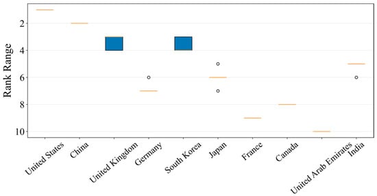
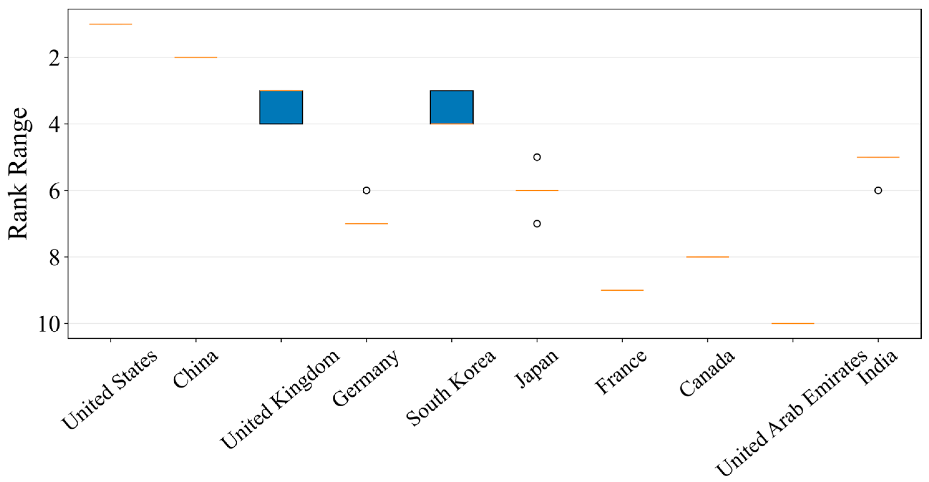
The sensitivity of the ranking results to the AHP–Entropy mixing parameter is then examined. The analysis is repeated under λ = 0.3, 0.5, and 0.7, and the resulting country rankings are re-evaluated. Figure 15 shows that the overall ranking pattern remains highly stable across the three settings, with no change in the leading positions and only minor local reordering among several middle-ranked countries. This observation is further confirmed by the pairwise Spearman rank correlations reported in Table 8, all of which remain above 0.97. These results indicate that the main conclusions of the proposed framework are robust to moderate changes in the mixing parameter.

Figure 15. Changes in country rankings under different AHP–Entropy mixing parameters.

Table 8. Pairwise Spearman rank correlations of country rankings under different λ settings.

λ	0.3	0.5	0.7
0.3	1.000	0.979	0.981
0.5	0.979	1.000	0.974
0.7	0.981	0.974	1.000

In addition to the ranking sensitivity, we further examine whether the representative Min-Variance investment strategy changes materially under alternative AHP–Entropy mixing parameters.

Table 9 shows that the terminal competitiveness level and annual variance remain close across $\mathrm{\lambda }=0.3$, $0.5$, and $0.7$, and the main funding priorities are largely preserved. Although some secondary allocation shares may vary moderately, the overall allocation pattern remains highly similar to that under the baseline setting $\mathsf{\lambda }=0.5$. These results suggest that the policy-oriented investment recommendation is not overly sensitive to moderate changes in the mixing parameter, which is consistent with the high-ranking stability reported in Table 8.

Table 9. Sensitivity of the representative Min-Variance investment strategy to alternative AHP–Entropy mixing parameters.

AHP–Entropy Mixing Parameter λ	Terminal Competitiveness Score	Annual Variance	Top Funded Indicators *	Allocation Similarity to the λ = 0.5 Strategy *
0.3	77.18	1.08 × 102	GPU Capabilities; Software Development Activity; AI Publications Count	0.973
0.5	77.43	1.00 × 102	GPU Capabilities; Software Development Activity; AI Publications Count	1.000
0.7	77.31	1.12 × 102	GPU Capabilities; Investment Amount; Software Development Activity	0.968

* Note: The allocation similarity is computed relative to the $\mathrm{\lambda }=0.5$ Min-Variance strategy. “Top funded indicators” reports the three indicators with the largest allocation shares under each $\mathrm{\lambda }$ setting.

7. Conclusions

This study proposes a causality-guided graph framework for the assessment, forecasting, and strategic optimization of national AI competitiveness. Based on the IPOE indicator system, the framework integrates hybrid weighting, dependency identification, graph-based evaluation, dynamic forecasting, and multi-objective resource allocation into a unified analytical pipeline. The results show that the proposed method captures both structural interactions and temporal evolution under limited-sample conditions. Under the baseline forecast, the United States and China remain the two leading economies, while the middle-ranked countries continue to experience visible reordering. The graph-based refinement further indicates that investment-related, innovation-related, and computing-related indicators play central roles in shaping national AI competitiveness. For China, the optimization results show that the Min-Variance strategy provides a balanced compromise between competitiveness improvement and policy stability under the assumed investment scenario.

Despite these contributions, several limitations remain. The analysis is still constrained by the limited scale of the annual sample, the ARIMA component mainly provides trend-consistent projections under short time series, and the investment-response mechanism relies on simplified marginal-cost and persistence assumptions. In addition, uncertainty propagation is treated in an approximate manner and may not fully capture correlated forecast errors across indicators. Future research may therefore extend the framework by incorporating broader cross-country datasets, more flexible temporal prediction models, and more data-driven calibration of policy-response relationships. Nevertheless, the proposed framework offers an interpretable and policy-oriented quantitative tool for assessing national AI competitiveness, forecasting its future evolution, and supporting long-term strategic decision-making under uncertainty.

References

- Zhang, B.; Zhu, J.; Su, H. Toward the Third Generation Artificial Intelligence. Sci. China Inf. Sci. 2023, 66, 121101. [Google Scholar] [CrossRef] [Scilit]
- Machucho, R.; Ortiz, D. The Impacts of Artificial Intelligence on Business Innovation: A Comprehensive Review of Applications, Organizational Challenges, and Ethical Considerations. Systems 2025, 13, 264. [Google Scholar] [CrossRef] [Scilit]
- Sun, T.; Li, R.; Wang, Q. From Algorithms to Sustainability: How AI Drives Renewable Energy Through Technology, Institutions, and Equity. Sustain. Dev. 2025. [Google Scholar] [CrossRef] [Scilit]
- Fatima, S.; Desouza, K.C.; Dawson, G.S. National Strategic Artificial Intelligence Plans: A Multi-Dimensional Analysis. Econ. Anal. Policy 2020, 67, 178–194. [Google Scholar] [CrossRef] [Scilit]
- National Science and Technology Council (NSTC); Select Committee on Artificial Intelligence. National Artificial Intelligence Research and Development Strategic Plan 2023 Update; Office of Science and Technology Policy (OSTP): Washington, DC, USA, 2023. [Google Scholar]
- European Parliament; Council of the European Union. Regulation (EU) 2024/1689 of the European Parliament and of the Council of 13 June 2024 Laying Down Harmonised Rules on Artificial Intelligence and Amending Relevant Regulations and Directives (Artificial Intelligence Act). Off. J. Eur. Union 2024, L1689, 1–144. [Google Scholar]
- Schrepel, T.; Pentland, A.S. Competition between AI Foundation Models: Dynamics and Policy Recommendations. Ind. Corp. Change 2025, 34, 1085–1103. [Google Scholar] [CrossRef] [Scilit]
- Erkkilä, T. Global Indicators and AI Policy: Metrics, Policy Scripts, and Narratives. Rev. Policy Res. 2023, 40, 811–839. [Google Scholar] [CrossRef] [Scilit]
- Ali, W.; Khan, A.Z. Factors Influencing Readiness for Artificial Intelligence: A Systematic Literature Review. Data Sci. Manag. 2025, 8, 224–236. [Google Scholar] [CrossRef] [Scilit]
- Jeon, G. Rethinking Competitiveness in the Age of AI: A Comparative Index-Based Approach. J. Int. Dev. 2025, 37, 1525–1542. [Google Scholar] [CrossRef] [Scilit]
- Shi, Y.F.; Tian, S.Y.; Chen, Y.J.; Cai, C.X.; Guan, H.H.; Li, X.J. Risk Assessment Method of Railway Engineering Technology Innovation in Complex Areas. Mathematics 2025, 13, 1970. [Google Scholar] [CrossRef] [Scilit]
- Yan, K.; Pang, X.; Li, Q.; Tian, G.; Dong, X. When does artificial intelligence innovation pay in servitization? A combined organizational learning and socio-technical systems perspective. J. Innov. Knowl. 2026, 14, 100960. [Google Scholar] [CrossRef] [Scilit]
- Wu, Y.; Li, M.; Liu, L.; Zhang, Y.; Liu, L.; Wang, L. Spatial-temporal allocation of regional land consolidation project based on landscape pattern and system dynamics. Cluster Comput. 2017, 20, 3147–3160. [Google Scholar] [CrossRef] [Scilit]
- Cheng, X.; Long, R.; Chen, H.; Li, Q. Coupling coordination degree and spatial dynamic evolution of a regional green competitiveness system-A case study from China. Ecol. Indic. 2019, 104, 489–500. [Google Scholar] [CrossRef] [Scilit]
- Al-Marzouqi, A.H.; Arabi, A.A. A Comparative Analysis of the Performance of Leading Countries in Conducting Artificial Intelligence Research. Hum. Behav. Emerg. Technol. 2024, 2024, 1689353. [Google Scholar] [CrossRef] [Scilit]
- Doshi, A.R.; Bell, J.J.; Mirzayev, E.; Vanneste, B.S. Generative artificial intelligence and evaluating strategic decisions. Strateg. Manag. J. 2025, 46, 583–610. [Google Scholar] [CrossRef] [Scilit]
- Hsueh, J.-T.; Lin, C.-Y. Integrating the AHP and TOPSIS decision processes for evaluating the optimal collection strategy in reverse logistic for the TPI. Int. J. Green Energy 2017, 14, 1209–1220. [Google Scholar] [CrossRef] [Scilit]
- Ho, W.; Ma, X. The state-of-the-art integrations and applications of the analytic hierarchy process. Eur. J. Oper. Res. 2018, 267, 399–414. [Google Scholar] [CrossRef] [Scilit]
- Xu, S.; Liu, Y. Research on the impact of carbon finance on the green transformation of China’s marine industry. J. Clean. Prod. 2023, 418, 138143. [Google Scholar] [CrossRef] [Scilit]
- Apichonbancha, P.; Lin, R.-H.; Chuang, C.-L. Integration of Principal Component Analysis with AHP-QFD for Improved Product Design Decision-Making. Appl. Sci. 2024, 14, 5976. [Google Scholar] [CrossRef] [Scilit]
- Dong, T.; Meng, L. Assessment of International Competitiveness of AI Industry Based on Positive and Negative Ideal Points Weighting Method. Mob. Inf. Syst. 2021, 2021, 9119262. [Google Scholar] [CrossRef] [Scilit]
- Hassija, V.; Chamola, V.; Mahapatra, A.; Singal, A.; Goel, D.; Huang, K.; Scardapane, S.; Spinelli, I.; Mahmud, M.; Hussain, A. Interpreting Black-Box Models: A Review on Explainable Artificial Intelligence. Cogn. Comput. 2024, 16, 45–74. [Google Scholar] [CrossRef] [Scilit]
- Ullah, N.; Khan, J.A.; De Falco, I.; Sannino, G. Explainable Artificial Intelligence: Importance, Use Domains, Stages, Output Shapes, and Challenges. ACM Comput. Surv. 2024, 57, 94. [Google Scholar] [CrossRef] [Scilit]
- Samek, W.; Montavon, G.; Lapuschkin, S.; Anders, C.J.; Müller, K.-R. Explaining Deep Neural Networks and Beyond: A Review of Methods and Applications. Proc. IEEE 2021, 109, 247–278. [Google Scholar] [CrossRef] [Scilit]
- Ma, X.; Hao, Y.; Li, X.; Liu, J.; Qi, J. Evaluating global intelligence innovation: An index based on machine learning methods. Technol. Forecast. Soc. Change 2023, 194, 122736. [Google Scholar] [CrossRef] [Scilit]
- Chun, Y.; Hur, J.; Hwang, J. AI technology specialization and national competitiveness. PLoS ONE 2024, 19, e0301091. [Google Scholar] [CrossRef] [Scilit] [PubMed]
- Garcia-Gastelum, T.S.; Uzeta-Obregon, C.R.; Álvarez-Carrillo, P.; León-Castro, E. An AI for Robust MCDM Ranking in a Large Number of Criteria. Mathematics 2025, 13, 2789. [Google Scholar] [CrossRef] [Scilit]
- Jin, H.; Tsai, F.S.; Martinez-Vazquez, J. Optimal expenditure decentralization for sustainable development: Evidence from a 52-country panel analysis. Financ. Innov. 2025, 11, 111. [Google Scholar] [CrossRef] [Scilit]
- Wang, Q.; Zhang, S.; Li, R. Artificial Intelligence in the Renewable Energy Transition: The Critical Role of Financial Development. Renew. Sustain. Energy Rev. 2026, 226, 116280. [Google Scholar] [CrossRef] [Scilit]
- Luo, H.; Jia, P.; Zhou, A.; Liu, Y.; He, Z. Bridge Node Detection between Communities Based on GNN. Appl. Sci. 2022, 12, 10337. [Google Scholar] [CrossRef] [Scilit]
- Bhattacharya, R.; Tripathi, S.; Nagwani, N.K. Detecting influential nodes with topological structure via Graph Neural Network approach in social networks. Int. J. Inf. Technol. 2023, 15, 2233–2246. [Google Scholar] [CrossRef] [Scilit]
- Stanford Institute for Human-Centered Artificial Intelligence. Artificial Intelligence Index Report 2025; Stanford University: Stanford, CA, USA, 2025; Available online: https://hai.stanford.edu/ai-index/2025-ai-index-report (accessed on 24 April 2026).
- Epoch AI. Data on the Trajectory of AI. Available online: https://epoch.ai/data (accessed on 20 January 2026).
- World Bank Group. World Development Indicators. Available online: https://databank.worldbank.org/source/world-development-indicators (accessed on 20 January 2026).
- Data Commons. Available online: https://www.datacommons.org/ (accessed on 20 January 2026).
- Center for Security and Emerging Technology. Data. Available online: https://cset.georgetown.edu/research-topic/data/ (accessed on 20 January 2026).
- Arena AI. Arena AI: The Official AI Ranking and LLM Leaderboard. Available online: https://arena.ai/ (accessed on 20 January 2026).
- Agarwal, C.; Queen, O.; Lakkaraju, H.; Zitnik, M. Evaluating Explainability for Graph Neural Networks. Sci. Data 2023, 10, 144. [Google Scholar] [CrossRef] [Scilit] [PubMed]
- Jiang, M.; Zhao, G.; Wang, X. Knowledge-Enhanced Spatiotemporal Network Based on Heterogeneous Graph Generation for Silicon Content Prediction in Blast Furnace. Adv. Eng. Inf. 2025, 68, 103689. [Google Scholar] [CrossRef] [Scilit]
Disclaimer/Publisher’s Note: The statements, opinions and data contained in all publications are solely those of the individual author(s) and contributor(s) and not of MDPI and/or the editor(s). MDPI and/or the editor(s) disclaim responsibility for any injury to people or property resulting from any ideas, methods, instructions or products referred to in the content. |
© 2026 by the authors. Licensee MDPI, Basel, Switzerland. This article is an open access article distributed under the terms and conditions of the Creative Commons Attribution (CC BY) license.