


Abstract
The Kimchi Premium—the persistent price wedge between Bitcoin on Korean and global exchanges—has resisted standard no-arbitrage explanations for over seven years, raising the question of how macro-financial shocks transmit into this segmented market. Prior work relies on static, linear estimators applied over short lag horizons, leaving the timing, nonlinearity, and regime dependence of the Premium’s adjustment largely untested. We address this gap using daily data from December 2017 to December 2025 () and rolling windows of 60, 120, and 240 trading days. Linear dynamics are tested with Granger causality (GC) and—because our return series are strongly leptokurtic (Bitcoin excess kurtosis , S&P 500 )—complemented by the Kraskov k-nearest-neighbor transfer entropy (TE) estimator, which captures conditional dependence in higher moments. Inference rests on a stationary bootstrap with pre-specified lag grids to avoid optimistic argmax bias, block-permutation tests for window-level detection rates, and Benjamini–Hochberg and Storey q-value corrections for multiple testing. Robustness is examined through conditional GC and conditional TE controlling for USD/KRW as a common factor, Toda–Yamamoto tests on price levels, a percentage-premium specification, a U.S. trading-day shift to address asynchrony, and winsorization sensitivity. We deliberately adopt a conservative inference stance at the panel level: window-level detection rates and pointwise bootstrap p-values are reported, but claims of “causality” are reserved for the within-window descriptive ranking of channels and horizons, with the panel-level null assessed by block-permutation and Benjamini–Hochberg corrections. Four empirical patterns emerge under this framing. First, Johansen tests identify a single cointegrating vector between Korean and global Bitcoin prices (trace vs. 5% critical value ), establishing the Premium as a stationary deviation from long-run parity, while none of the four macro indicators cointegrate with global Bitcoin. Second, GC detection rates for the Premium concentrate at the 240-day horizon: Gold → Premium reaches (95% Wilson CI ), KOSPI 200 → Premium , and USD/KRW → Premium . Third, the Kraskov TE reveals an asymmetry invisible to linear tests: for Gold → Premium at , the median optimal lag is five days, against one day for Gold → Bitcoin (chi-square ). Percentage-premium detection rates are substantially higher (e.g., for Gold → Premium at ), indicating that the dollar-wedge specification understates causal strength. Fourth, block-permutation tests do not reject the global null of no window-level excess rejection, and Benjamini–Hochberg rejects no pair at ; we therefore read the detection-rate evidence as descriptive of localized, crisis-dependent transmission episodes rather than as panel-level rejection of pointwise non-causality, and the paper’s contribution is accordingly positioned at the level of channel ranking, lag structure, and regime decomposition rather than at the level of blanket causality claims. Crisis decomposition shows transmission is concentrated in the ETF-Halving regime ( mean GC detection) and below during the Terra–Luna () and Russia–Ukraine () episodes. The findings situate the Premium as a stationary error-correction term whose adjustment is dominated by exchange-rate and commodity channels rather than U.S. equities, with implications for arbitrage models, regulatory monitoring, and information-flow analyses of segmented crypto markets.
Keywords:
Bitcoin; Kimchi Premium; Granger causality; transfer entropy; rolling-window analysis; market segmentation MSC:
62M10; 94A17; 62P05; 91B84
1. Introduction
Cryptocurrency markets have grown into a significant component of the global financial system, with Bitcoin in particular sustaining high trading volumes on major exchanges. South Korea stands out among national markets for its distinctive pricing dynamics: it is consistently among the most active national markets in cryptocurrency by trading volume despite the relatively small size of its domestic population. A distinctive feature of the Korean cryptocurrency market is the persistent price differential between domestic and international exchanges, known as the “Kimchi Premium,” which has important implications for market efficiency, regulatory policy, and cross-border capital flows.
The Kimchi Premium refers to the systematic price difference between Bitcoin traded on South Korean exchanges (primarily Upbit and Bithumb) and those traded on global platforms. Since its emergence in 2017, this premium has exhibited substantial variation in magnitude across periods of differing demand and arbitrage capacity [1]. Unlike temporary arbitrage opportunities that quickly disappear in efficient markets, the Kimchi Premium has persisted for years, suggesting structural factors beyond simple market inefficiencies. This phenomenon is particularly significant for three stakeholder groups: arbitrageurs seeking profit opportunities constrained by capital controls and settlement delays; investors needing to understand the segmentation between Korean and global cryptocurrency markets; and policymakers concerned with capital flow regulations and financial market integration.
The persistence of the Kimchi Premium challenges conventional financial theory, which holds that arbitrage mechanisms should rapidly eliminate cross-market price discrepancies. This enduring anomaly is largely driven by structural frictions within the Korean cryptocurrency market. Ref. [2] argue that capital controls amplify existing frictions from the microstructure of the Bitcoin network, thereby sustaining persistent price differentials. Korean cryptocurrency exchanges require government-issued identification and domestic bank accounts for KYC and AML compliance, effectively preventing participation by foreign arbitrageurs. In addition, fiat transfers typically require two to five business days to settle, whereas Bitcoin transactions are completed within 30 to 60 min, exposing arbitrageurs to substantial price risk during the interim [3]. These institutional and operational frictions segment the Korean market from global liquidity flows, allowing domestic demand and supply conditions to diverge significantly from international price dynamics.
Prior research has identified correlations between the Kimchi Premium and a small set of microstructure and behavioral variables. Choi et al. [2] document that the Kimchi Premium is positively related to Bitcoin price volatility, transaction fees, and blockchain confirmation times, while Eom [1] attributes premium fluctuations to speculative trading and arbitrage constraints. However, existing studies have three critical limitations. First, they employ static models over fixed time periods, failing to capture how relationships evolve during different market regimes. Second, they test limited lag structures (typically 1–5 days), potentially missing longer-term dependencies arising from settlement delays and regulatory frictions. Third, they rely exclusively on linear methods, such as Granger causality, which may fail to detect nonlinear dependencies that transfer entropy can identify [4,5].
This study addresses these gaps by investigating the time-varying causal relationships between the Kimchi Premium and major financial indicators over an extended sample (1 December 2017 to 30 December 2025; trading days) using a rolling-window design with three horizons ( trading days). The empirical framework combines four estimators—Granger causality, histogram transfer entropy, the Kraskov k-nearest-neighbor transfer entropy [6], and the Toda–Yamamoto level-series test—with explicit multiple-testing corrections (block permutation, Benjamini–Hochberg FDR, Storey q-values) and five complementary robustness exercises detailed in Section 3. Full technical details of the new estimators and multiplicity corrections are deferred to Section 3.5, Section 3.6, Section 3.7, Section 3.8, Section 3.9, Section 3.10 and Section 3.11.
Our analysis focuses on four principal financial indicators representing both global and domestic market dynamics: the S&P 500 Index as a proxy for global risk appetite, gold prices (iShares Gold Trust) as a safe-haven indicator, the KOSPI 200 Index capturing Korean equity market sentiment, and the USD/KRW exchange rate affecting cross-border arbitrage costs. By examining how these variables influence both global Bitcoin prices and the Kimchi Premium with varying lag structures, we identify the transmission mechanisms and adjustment speeds that characterize segmented cryptocurrency markets.
This study yielded four principal findings. First, Johansen cointegration tests confirm a single cointegrating vector between Korean and global Bitcoin prices (trace vs. 5% critical value ), so the Premium is best interpreted as a mean-reverting deviation from long-run parity rather than a free parameter. None of the four macroeconomic predictors cointegrate with global Bitcoin, locating their role in short-run transmission rather than long-run pricing. Second, detection rates for the Premium are highest at the 240-day horizon and for commodity and exchange-rate channels: Gold → Premium reaches of rolling windows, USD/KRW → Premium , and KOSPI 200 → Premium ; the corresponding rates for the global Bitcoin target are lower (10–). Third, the asymmetry between Bitcoin and the Premium in adjustment speed is visible primarily in Kraskov nonlinear TE: for Gold → Premium at , the median optimal lag is five days versus one day for Gold → Bitcoin (chi-square ). Fourth, block-permutation tests on window-level detection rates yield p-values concentrated in , and no pair survives a Benjamini–Hochberg correction at —a deliberately conservative finding we report rather than conceal, and which leads us to interpret the detection-rate evidence as descriptive of localized transmission episodes rather than as a global rejection of non-causality.
This study makes three contributions relative to the closest prior work. First, Eom [1] documents static correlations between the percentage Kimchi Premium and trading volume/volatility over a pre-2020 sample using linear regression, and Choi et al. [2] identify microstructure frictions (transaction costs, confirmation time, volatility) as the main drivers of the Premium in a full-sample time-series regression. Neither paper addresses how these relationships evolve around the COVID-19, Terra–Luna, FTX, Russia–Ukraine, and 2024 ETF-Halving episodes. Our rolling-window design, coupled with explicit crisis decomposition, reveals that transmission is not stationary over the sample—nearly all of the 240-day GC detection events are concentrated in the ETF-Halving regime ( mean detection) and in the “Normal” residual (), with near-zero rates during the three intermediate crises. Second, Jo et al. [3] characterize arbitrage profitability under deterministic transaction and settlement costs but do not test the statistical asymmetry in adjustment speeds. We test this asymmetry formally with chi-square and Mann–Whitney U statistics on lag distributions and document that the asymmetry is systematically detectable only under a nonlinear (Kraskov k-NN) information-theoretic estimator—evidence that the arbitrage-settlement friction in [3] leaves a signature outside the reach of linear Granger tests. Third, relative to the broader transfer entropy finance literature [7,8,9,10], we contribute a conditional extension (conditional GC and conditional TE controlling for USD/KRW as a common factor) that shows the Premium channels are not artifacts of a shared FX driver: the conditional detection rate for KOSPI 200 → Premium at increases from (unconditional) to (conditional on USD/KRW), consistent with true direct transmission.
The remainder of this paper is organized as follows. Section 2 reviews the literature on cryptocurrency markets, the Kimchi Premium, and causal inference methods. Section 3 describes the rolling-window methodology and lag selection procedures. Section 4 presents the data sources, sample construction, and descriptive statistics. Section 5 reports the empirical results of time-varying causality and optimal lag structures. Section 6 discusses the economic interpretation and policy implications. Section 7 concludes.
2. Literature Review
2.1. Cryptocurrency Markets and Price Drivers
Cryptocurrency markets represent a fundamental departure from traditional financial systems through three defining characteristics: decentralized governance structures, continuous 24/7 trading operations, and extreme price volatility. Unlike conventional assets governed by central authorities and regulatory frameworks, cryptocurrencies operate on distributed ledger technology without centralized control over monetary policy or market intervention mechanisms. This structural difference creates unique price dynamics that challenge traditional asset pricing models.
The determinants of Bitcoin prices have been extensively studied with mixed conclusions about their primary drivers. Baur et al. [11] analyze the statistical properties of Bitcoin and find that it is largely uncorrelated with traditional asset classes such as stocks, bonds, and commodities both in normal times and in periods of financial turmoil; their analysis of transaction-level data leads them to conclude that Bitcoin is mainly used as a speculative investment rather than as a medium of exchange. Corbet et al. [12] examine how macroeconomic news announcements affect cryptocurrency returns and find evidence of heightened price sensitivity to policy-relevant information events relative to traditional asset classes.
Sentiment, attention, and behavioral factors are an active line of inquiry alongside macroeconomic determinants. Lee et al. [13] and An et al. [14] discuss the role of investor attention, social-media activity, and news coverage in shaping cryptocurrency returns; Griffith et al. [15] provide complementary evidence in the equity context, showing that media-derived sentiment measures (fear, gloom, joy) predict short-horizon stock returns and volatility. Makarov and Schoar [16] survey the institutional architecture of cryptocurrencies and decentralized finance and discuss the limited integration of crypto-asset prices with conventional monetary-policy transmission. Härdle et al. [17] and Hairudin et al. [18] review the cryptocurrency-market literature and emphasize the decentralized governance and market-microstructure features that distinguish crypto trading from traditional financial markets.
2.2. Bitcoin’s Relationship with Traditional Financial Markets
Dyhrberg [19] explores Bitcoin’s hedging properties using an asymmetric GARCH framework and concludes that Bitcoin can serve as a hedge against the FTSE stock index and as a short-run hedge against the U.S. dollar, sharing some hedging capabilities with gold. The classification of Bitcoin as commodity-like versus currency-like is therefore conditional on horizon and reference asset.
Bouri et al. [20] apply a dynamic conditional correlation model and conclude that Bitcoin is best characterized as a diversifier rather than a hedge or safe haven against major world stock indices, bonds, oil, gold, the general commodity index, and the U.S. dollar; safe-haven properties are confined to weekly extreme down moves in Asian equity markets.
Recent studies revisit the link between Bitcoin and macroeconomic fundamentals as cryptocurrency markets have matured. Wang et al. [21] examine short- and long-term interactions between Bitcoin and U.S. macroeconomic variables and find evidence of an evolving relationship that lends some support to the “digital gold” interpretation. Wahyuni et al. [22] apply a dynamic conditional correlation MGARCH framework to monthly U.S. inflation, interest-rate, USD/EUR, gold, and Bitcoin data, and report a negative association of Bitcoin price with inflation, interest rates, and the USD/EUR rate alongside a positive association with the gold price. Karkera and Sudarkodi [23] review the determinants of Bitcoin volatility and emphasize the role of investor sentiment relative to traditional fundamentals. Kim et al. [24] analyze the potential introduction of cryptocurrency indices into the U.S. ETF market and argue, from systemic-risk and mean-variance perspectives, that such indices could function as alternative asset classes within diversified portfolios. Beyond the asset-pricing literature, Dupuis et al. [25] survey the broader crypto-asset ecosystem from an audit and accounting standpoint, providing context for the institutional and reporting environment in which cross-border cryptocurrency trading takes place.
2.3. The South Korean Cryptocurrency Market Context
South Korea’s cryptocurrency market exhibits distinctive characteristics shaped by its regulatory environment, technological infrastructure, and investor demographics. Korea has long been one of the most active national markets for crypto-asset trading, a position that reflects the country’s high level of technological adoption, the prominence of retail participation in domestic exchanges, and a regulatory framework that constrains cross-border arbitrage. These structural features are documented in detail by [2,26,27] and provide the institutional context for the persistence of the Kimchi Premium.
The KOSPI 200 index is the principal benchmark for Korean equity-market performance and is a natural reference point for domestic cryptocurrency investment behavior. Lee et al. [28] document that Bitcoin prices in Korea are driven more by investor-attention and psychological variables (search trends, frequency of Bitcoin-related news articles) than by conventional supply, demand, or real-economic fundamentals. Empirical analyses of Korean cryptocurrency trading more broadly [29] have likewise emphasized investor-attention and macro-economy variables as joint determinants of price changes. In the Korean equity context, Nam and Seong [30] use causality analysis on financial-news flows to show that information transmission between firms in the Korean stock market is detectable and improves return prediction, providing methodological support for the kind of information-flow analysis we apply to the cross-border Bitcoin market.
Exchange-rate dynamics introduce an additional channel through which the Korean cryptocurrency market is connected to the global financial system. Park and Son [31] examine cross-country dollarization and the joint dynamics of inflation and foreign-exchange markets, providing context for how won depreciation can shift demand for foreign-currency-denominated assets. Choi [32] and Choi and Kim [8] analyze international capital flows and information flow across financial markets and document that capital movements respond to both domestic policy and global risk conditions, generating feedback dynamics between exchange rates and cross-border asset pricing. Zhao et al. [33] further document that geopolitical and trade-policy shocks propagate to the exchange-rate system linking the KRW, JPY, and CNY, providing additional motivation for treating USD/KRW as a key conditioning variable in our analysis.
Regulatory frictions fundamentally shape the Korean cryptocurrency ecosystem. Capital controls cap annual cross-border retail transfers (the standard threshold being $50,000 without additional documentation requirements) and Korean exchanges implement strict KYC/AML requirements that mandate government-issued identification and domestic bank accounts, effectively excluding most non-resident arbitrageurs from the domestic order book [34,35]. Banking-side restrictions on international wire transfers add further frictions, since few domestic banks offer cryptocurrency-related settlement services. These regulatory barriers create market segmentation that enables persistent price differentials between domestic and international markets.
2.4. The Kimchi Premium Phenomenon
The Kimchi Premium represents a persistent pricing anomaly specific to Korean cryptocurrency markets, defined as the percentage difference between Bitcoin prices on Korean exchanges (primarily Upbit and Bithumb) and global platforms. Since its emergence in 2017, this premium has displayed remarkable persistence in magnitude, with Eom [1] documenting its association with speculative trading activity and volatility on the Korean side. Unlike temporary arbitrage opportunities that characterize efficient markets, the Kimchi Premium has persisted for several years, suggesting structural rather than transient causes.
Three categories of factors sustain the premium according to existing research. First, regulatory barriers prevent efficient arbitrage: Han [26] and Oh [27] identify capital controls and the associated compliance burden as the primary friction. Second, operational constraints limit arbitrage capacity, since cross-border transfers settle on a multi-day fiat-banking cycle while opportunity windows on the cryptocurrency side close in minutes. Third, market microstructure features affect price formation: Choi et al. [2] document that transaction costs, blockchain confirmation time, and Bitcoin price volatility are positively associated with the size of the Korean Bitcoin premium, consistent with delay-and-price-risk frictions on the arbitrageur side. Jo et al. [3] study statistical-arbitrage opportunities in the cross-border cryptocurrency market by relating the Kimchi Premium to exchange-rate dynamics, using both linear regression and an LSTM-based predictor of the won exchange rate to identify state-dependent profit windows. Their analysis treats the cost structure as fixed and does not consider how arbitrage capacity itself might vary with market conditions or regulatory changes.
2.5. Research Gaps
Critical examination of the existing literature reveals three fundamental gaps that limit understanding of Kimchi Premium dynamics. First, prior research employs static models estimated over fixed time periods, assuming constant relationships between variables. Eom [1] examines the relationship between the Kimchi Premium, trading volume, and volatility, arguing that elevated volume and enhanced uncertainty are associated with larger premiums. Financial markets experience regime changes during crises, regulatory shifts, and technological developments that alter causal relationships. The COVID-19 pandemic, cryptocurrency regulatory changes in 2021, and the 2022 global inflation shock likely modified how financial variables affect the Kimchi Premium, but static models cannot capture these evolving dynamics.
Second, existing studies test limited lag structures without systematic optimization. Most prior research examines short lags (typically up to one week) based on convention rather than data-driven selection. Because the institutional infrastructure underlying cross-border arbitrage—fiat-banking settlement cycles, blockchain confirmation delays, and periodic regulatory reporting—operates on heterogeneous time scales, relevant lag structures may extend well beyond one week. The failure to test longer lags may miss important medium-term relationships, particularly for variables like exchange rates that affect the Premium through multiple channels including trade flows, capital movements, and investor sentiment.
Third, the literature relies exclusively on linear methods, primarily Granger causality and VAR models, which assume constant linear relationships between variables. Cryptocurrency markets exhibit well-documented nonlinearities including threshold effects, regime switches, and asymmetric responses to positive versus negative shocks. Transfer entropy can detect nonlinear dependencies that Granger causality misses [4], potentially revealing hidden relationships. Barnett et al. [5] prove that for Gaussian variables, transfer entropy and Granger causality are equivalent, but cryptocurrency returns violate normality assumptions with excess kurtosis exceeding 10 and significant skewness, making nonlinear methods essential. Transfer entropy has been successfully applied to equity indices [7,8,36], foreign exchange markets [10,37], and commodity futures [9], demonstrating its effectiveness in capturing nonlinear dependencies in non-Gaussian financial data.
2.6. Theoretical Channels of Transmission
The Kimchi Premium is the price wedge between the domestic KRW-denominated price converted at the spot rate and the global USD price. Four economic channels can shift this wedge: (i) an exchange-rate channel in which innovations in mechanically enter the wedge through the conversion term, so the Premium should co-move with USD/KRW at short lags and also inherit longer-horizon pass-through via import-sensitive Korean macro conditions [38,39]; (ii) an equity-substitution channel in which Korean retail investors reallocate between KOSPI 200 and Upbit/Bithumb Bitcoin as domestic attention and sentiment toward the two risk assets shift [28,34], producing a lead–lag from equity flows to the Premium; (iii) a global risk-appetite channel in which the S&P 500 and gold capture the state of international risk pricing, with effects on the Premium mediated through capital-flow frictions that delay the domestic response relative to the global Bitcoin response [11,20,32]; and (iv) an arbitrage-capacity channel in which the $50,000 annual cross-border retail remittance limit and two-to-five business-day fiat settlement cycle [3,35] bound the speed at which the Premium can mean-revert toward zero. Channels (i)–(iii) predict nonzero short-run causality from the listed predictors into the Premium; channel (iv) predicts that the Premium’s response to any shock should lag the global Bitcoin response by at least the settlement horizon, which is the origin of the adjustment-speed asymmetry that Hypothesis H3 below formalizes and that Section 5.3 documents in the Kraskov TE.
3. Methodology
3.1. Research Design Overview
Let denote a complete probability space equipped with a discrete-time filtration satisfying the usual conditions of right-continuity and completeness. We observe six adapted stochastic processes on this space: the global Bitcoin return , the Kimchi Premium return , and four financial indicator returns for . All processes are assumed strictly stationary and ergodic on each estimation window, verified by the augmented Dickey–Fuller test at the 1% level.
The research design employs a rolling-window approach on daily data from 1 December 2017 to 30 December 2025, comprising trading days defined by the union calendar of conventional markets—all calendar dates on which either the Korean markets (KOSPI 200, USD/KRW) or the U.S. markets (S&P 500, IAU) were open. Bitcoin trades continuously and is aligned to this union trading calendar. This span covers the COVID-19 pandemic, the Terra–Luna collapse (May 2022), the FTX failure (November 2022), the Russia–Ukraine war, and the U.S. spot-Bitcoin-ETF approval and 2024 halving episode.
The study combines two linear and two nonlinear causality measures. Granger causality (GC) operates on the conditional mean vs. under a linear parametric specification, detecting predictive relationships in the first moment. Toda–Yamamoto (TY) GC extends this to price levels by adding one redundant lag (), yielding a distribution robust to the possible presence of unit roots [40]. Transfer entropy (TE) quantifies the Kullback–Leibler divergence between the full conditional and the marginal conditional , capturing dependencies across the entire conditional distribution—including higher moments, threshold effects, and volatility spillovers—without parametric assumptions. We estimate TE both with a Freedman–Diaconis histogram and with the Kraskov k-nearest-neighbor (KSG) estimator [6] with , which avoids the positive discretization bias of the histogram in short windows. Barnett et al. [5] prove that for a stationary Gaussian VAR(p) process with finite p, (in nats). Because cryptocurrency returns violate the Gaussian assumption (excess kurtosis for Bitcoin and for the S&P 500; see Section 4.4), this equivalence fails, and the two measures yield complementary information. Finally, Johansen cointegration tests are applied to the non-stationary level pair and to each predictor with global Bitcoin, to separate long-run equilibrium from short-run transmission (Section 4.6).
3.2. Variable Selection
The analysis examines four financial indicators representing distinct transmission channels. The S&P 500 Index functions as the main indicator for U.S. stock market performance and worldwide risk assessment. The iShares Gold Trust (IAU) uses gold spot prices to monitor worldwide risk avoidance and safe-haven investment needs. The KOSPI 200 Index captures Korean equity market performance through the market-capitalization-weighted average of the 200 largest companies listed on the Korea Exchange. The USD/KRW exchange rate impacts cryptocurrency markets through different transmission channels because changes in exchange rates modify the Bitcoin price on international trading platforms, which affects arbitrage opportunities.
3.3. Granger Causality Test
Bivariate VAR representation. Let denote a bivariate, covariance-stationary process with . The reduced-form VAR(p) model is
where is the intercept vector, is the coefficient matrix at lag k, is a white-noise innovation process, and is a positive-definite covariance matrix. The process is stable if and only if all eigenvalues of the companion matrix lie strictly inside the unit circle, for . In partitioned form, each equation reads as follows:
Granger non-causality and likelihood-ratio test. X does not Granger-cause Y if and only if conditioning on the past of X does not reduce the mean-squared prediction error of Y: , where [41]. In the VAR framework, this is equivalent to the joint restriction
We test using the Sims-corrected likelihood-ratio statistic [42]:
where is the number of estimated parameters per equation (providing a finite-sample degrees-of-freedom correction), is the restricted residual covariance matrix (under ), and is its unrestricted counterpart. Under and Gaussian innovations, as .
Wold representation and spectral Granger causality. Under stability, admits the Wold moving-average representation , where the transfer-function matrices are computed recursively from with . Define the spectral density matrix as the discrete-time Fourier transform of the autocovariance sequence:
where is the transfer function and * denotes the conjugate transpose. Following [42], the spectral GC from Y to X at frequency is
where is the -element of , is the -element of , and is the innovation variance of X. The total time-domain GC decomposes as , which satisfies [42]. Positive values of at specific frequencies identify whether causal influence operates through high-frequency (short-term) or low-frequency (long-term) channels.
3.4. Optimal Lag Selection Procedures
Optimal lag selection ensures validity and power of causality tests: under-specification omits true dynamics, whereas over-specification inflates estimation variance and erodes power. For a k-dimensional VAR(p), the total number of freely estimated mean parameters is (each of k equations contains one intercept and lag coefficients). In the bivariate case (), . The optimal lag minimizes one of three information criteria [41]:
where is the maximum-likelihood covariance estimator and for . The AIC is efficient (minimizes one-step-ahead forecast error), the BIC is consistent (selects the true p with probability one as when the DGP has finite order), and the HQIC balances both properties under penalization.
The lag selection follows a majority-voting protocol. Define , , as the respective minimizers. If at least two criteria agree—i.e., —that common value is selected. If all three disagree, is chosen to prioritize parsimony. Monte Carlo simulations confirm that this rule yields consistent lag identification in approximately 92% of cases for .
Lag ranges are constrained by the rolling-window length w to maintain at least effective observations per parameter. Requiring yields
giving , , and .
3.5. Transfer Entropy Computation
Information-theoretic definition. Transfer entropy (TE) is the conditional mutual information that quantifies the directional flow of information from X to Y at lag ℓ, without imposing parametric assumptions on the data-generating process [4]. Define the random vectors , , and . The TE from X to Y at lag ℓ is
where denotes conditional mutual information and is the Kullback–Leibler divergence, both measured in bits (). By construction, , with equality if and only if (conditional independence).
For continuous random variables with jointly absolutely continuous distributions, Equation (12) expands as
Discrete estimator and bias correction. For empirical estimation, we discretize the state space via histogram binning. Let denote a partition of the range of variable Z into bins. The plug-in estimator is
where is the empirical joint probability. The plug-in estimator is positively biased in finite samples. For T observations, the leading-order bias is [4]. The bias diminishes as at rate and is further controlled by our bootstrap inference procedure (Section 3.7).
Bin widths are determined by the Freedman–Diaconis rule:
where is the interquartile range of Z, yielding bins. For a typical cryptocurrency return series with and , this produces and –15 bins per variable, balancing granularity against statistical stability.
Nonparametric k-nearest-neighbor estimator. Histogram plug-in estimators discretize the sample space and are known to have an upward bias of order in short windows [4,6]. As a robustness check we additionally estimate TE with the Kraskov–Stögbauer–Grassberger (KSG) k-nearest-neighbor estimator [6], which writes the TE as a difference of two mutual data points and estimates each via
where is the digamma function, k is the number of neighbors (we use ), is the count of A-marginals within the Chebyshev -ball determined by the k-th nearest neighbor in the joint space, and analogously for . KSG has the convenient property that discretization artifacts cancel between the two mutual-information terms, yielding near-zero bias in small samples at the cost of a higher variance. The choice of window at which to apply KSG involves a bias–variance tradeoff that is sharper than it first appears. At the histogram plug-in bias is largest, which is the originally flagged concern; but KSG at the same window suffers from a severe variance penalty because a neighbor search over only 60 observations distributed across a 20-day lag reach effectively uses ∼40 neighbor pairs per density estimate, and the resulting detection-rate series is dispersed around both the histogram and the GC benchmarks in a way that is uninformative rather than bias-corrected. We therefore apply KSG at , on the grid , where both its bias-cancellation advantage and its variance properties are most favorable and where the KSG–histogram discrepancy is diagnostic rather than noise-dominated; the histogram estimator is retained at as one piece of evidence in a multi-estimator comparison rather than as a stand-alone causal inference. This is a deliberate methodological choice and is flagged transparently in the Discussion as a limitation of the histogram-only evidence at the shortest window.
Optimal lag selection on a pre-specified grid. The naive procedure of selecting over all lags and then bootstrapping a p-value at that suffers from a well-known selection bias: the maximum of dependent statistics is skewed upward under the null, so the resulting p-value is optimistic in proportion to . Following the reviewers’ suggestion to make lag selection pre-specified rather than data-driven, we evaluate TE on a small, economically-motivated grid
corresponding to daily, near-term-arbitrage, one-week-settlement, two-week and one-month horizons. For each lag we compute the stationary-bootstrap p-value of Section 3.7. The TE-detection event for a window is (Bonferroni inside the grid), and the optimal lag conditional on detection is . If no lag satisfies the significance constraint, we set .
Equivalence theorem and its failure under non-normality. Barnett et al. [5] prove that for a stationary, jointly Gaussian VAR(p) with finite p, TE measured in nats satisfies the exact identity
where and are the conditional prediction error variances of the restricted and unrestricted regressions, respectively. This equivalence rests on two conditions: (i) joint Gaussianity, so that the conditional distribution is fully determined by its mean and variance; and (ii) finite VAR order, so that p lags capture all relevant history. Our data violate condition (i): Bitcoin returns exhibit excess kurtosis of 7.29 and the S&P 500 reaches 14.77 (see Section 4.4). Under non-Gaussianity, TE captures dependencies in higher conditional moments—including volatility clustering, threshold effects, and tail co-movements—that GC, as a first-moment test, cannot detect.
3.6. Rolling-Window Framework
The rolling-window estimator replaces the assumption of time-invariant parameters with the weaker assumption of local stationarity: within each window , the data-generating process is treated as covariance-stationary and ergodic, while parameters are permitted to change across windows. For the full sample of trading days, we construct overlapping windows for each of three window lengths . To control compute cost while preserving the overlapping-window smoothness of the detection-rate series, we evaluate every fifth window (stride ). The reported detection rates therefore refer to the number of evaluated windows within each stride: for , 398 for , and 374 for .
The window lengths are chosen to span economically interpretable horizons while satisfying a minimum degrees-of-freedom constraint. Denote the window-specific lag bound by from Equation (11). The three specifications yield
For each window , the estimation protocol proceeds as follows:
- 1.
- Stationarity verification. Apply the ADF test with Schwarz-criterion lag selection; reject the unit-root null at the 1% level. If any series is non-stationary within the window, take first differences and re-test.
- 2.
- GC estimation. For each lag order , estimate the VAR(p) in Equation (1) by OLS, compute from Equation (5), and select via the majority-voting IC rule (Section 3.4).
- 3.
- TE estimation. For each lag (with ), compute from Equation (14) with Freedman–Diaconis binning.
- 4.
- Significance assessment. Compute from Equation (21) with replications (sufficient for a p-value resolution at ) for both GC and TE at the selected optimal lags.
- 5.
- Output. Record the tuple for each of the eight directional relationships (4 predictors × 2 targets).
The total computational budget is model estimations per window length. With three window lengths, the full analysis requires approximately model fits, completed in under thirty minutes on an eight-core workstation.
3.7. Statistical Inference via Stationary Bootstrap
Although GC p-values can be computed from the asymptotic distribution of Equation (5), no closed-form distribution exists for the TE plug-in estimator under dependence. To ensure inferential comparability between the two methods, we adopt a unified resampling framework—the stationary bootstrap of [43]—for both GC and TE.
Bootstrap algorithm. Let , , denote the observed bivariate series within a given rolling window. The stationary bootstrap draws blocks of random, geometrically distributed length: at each step t, a new block begins with probability by drawing a uniform starting index ; otherwise, the block continues to the next observation (wrapping circularly). The mean block length is . Following the Hall–Horowitz–Jing (HHJ) criterion [44], we set , yielding trading days. The HHJ rule minimizes the mean squared error of the bootstrap variance estimator:
where is the bootstrap sample mean. Politis and Romano [43] prove that, for stationary, -mixing sequences with for some , the bootstrap distribution of a smooth functional converges weakly in probability to the true sampling distribution.
For each bootstrap replicate (with ), we construct a resampled series and compute the test statistic —either from Equation (5) or from Equation (14). The bootstrap p-value is
where is the statistic from the original sample and is the indicator function. This yields a nonparametric, distribution-free significance level valid under serial dependence. Monte Carlo evidence in prior literature supports that the stationary bootstrap with HHJ-selected blocks maintains nominal size () and achieves accurate coverage probabilities under dependence.
3.8. Johansen Cointegration and Toda–Yamamoto Granger Test
The GC and TE tests described above operate on returns, which are stationary. As a complement, we assess the level series directly. Johansen’s reduced-rank procedure [45] provides a test for the cointegration rank r in the VECM
where , is the cointegration rank, and , are the loading and cointegrating matrices. The trace statistic tests against the unrestricted alternative. Critical values are taken from [46].
In systems where (no cointegration) but where levels may nevertheless be individually , the Toda–Yamamoto (TY) procedure [40] provides a Granger-causality test robust to unit roots. Given the optimal lag p selected from the stationary return transformation, we fit a VAR() on the level series where is the presumed maximum order of integration (here ). The causality test is a Wald test on the first p coefficients of the predictor in the target equation; the extra lags act as auxiliary regressors that restore the standard asymptotic distribution.
3.9. Spectral-Frequency Decomposition of Granger Causality
The time-domain Granger statistic of Equation (5) aggregates predictive content across all frequencies. Following [42], we decompose this aggregate into a frequency-specific causality density
where is the spectral-density matrix of the VAR innovations, is the transfer function, and is the innovation covariance. Integrating across recovers the time-domain statistic exactly. To summarize the decomposition economically, we integrate over three frequency bands defined by their period-day support: short (period < 5 days), medium (5–20 days), and long (≥20 days). These bands correspond loosely to daily-arbitrage, weekly-settlement, and monthly-macro horizons.
3.10. Conditional Granger Causality and Conditional Transfer Entropy
A common concern in bivariate causality testing is that a detected link may be spuriously driven by a third variable Z correlated with both. Because USD/KRW enters the definition of the Kimchi Premium through the exchange-rate conversion, it is the most natural candidate for a common-factor proxy. Following [47], we augment each bivariate VAR with Z-lags and test
which is distributed under the null of no conditional causality. The analogous conditional transfer entropy is
estimated nonparametrically with the same KSG formula of Equation (16) but on the augmented state . A decrease in the detection rate of after conditioning on Z identifies Z as an important common driver; an increase (as we observe for several pairs) indicates that controlling for Z sharpens rather than weakens the direct channel.
3.11. Multiple-Testing Correction
The rolling-window detection rate is itself a composite test statistic: it aggregates correlated window-level tests. The sampling distribution of under the global null : no causality in any window is not the binomial , because the window-level p-values are strongly serially dependent through the overlapping observations. We therefore assess against a block-permutation null: we form independent permutations of the predictor series by sampling blocks of length 20 trading days, re-estimate the detection rate for each permutation, and report
as the empirical one-sided p-value for the detection rate.
The panel of 56 permutation p-values across (predictor × target × window × estimator) configurations is then subjected to two complementary multiplicity corrections: the step-up procedure of Benjamini and Hochberg [48] controlling the false discovery rate (FDR) and the q-value procedure of Storey [49], which is adaptive to the unknown proportion of true nulls . Methodologically related applications of time-varying Granger causality [50] and information-theoretic risk-boundary analysis [51,52] provide additional context for the rolling-window inference apparatus we deploy here. A configuration is reported as significant after multiple-testing correction when its Benjamini–Hochberg-adjusted q-value is below .
3.12. Hypothesis Testing Framework
The empirical analysis evaluates three hypotheses, each tested with explicit rejection criteria, effect-size quantification, and distributional assumptions.
Hypothesis 1 (Existence of Causality).
For each predictor and target , define the empirical rejection rate as the proportion of rolling windows in which the null of non-causality is rejected at level :
where denotes the number of rolling windows and is the bootstrap p-value from Equation (21) in window t. Under the global null of no causality in any window, converges to by the law of large numbers; the hypothesis is supported when , substantially exceeding the nominal false-rejection rate. Confidence intervals for are constructed via the Wilson score interval at the 95% level. Because is a composite of correlated window-level tests, we additionally assess it against a block-permutation null (block length 20 trading days, ) that preserves the serial dependence of the predictor while destroying the predictor–target linkage, and control the resulting panel of p-values for multiplicity across the 56 comparisons by both the Benjamini–Hochberg step-up and Storey’s q-value procedures.
Hypothesis 2 (Time-Varying Causality).
Let denote the set of crisis-period window centers (COVID-19: 1 March–31 December 2020; Russia–Ukraine: 24 February–31 August 2022) and the normal periods. For each pair, extract the vectors of selected optimal lags and partition them into crisis (, size ) and normal (, size ) subsamples. The Mann–Whitney U statistic tests whether the two populations share a common median:
where is the rank of the i-th crisis observation in the combined sample. Under the null of identical distributions, the standardized statistic , where , converges to for large . A tie-corrected variance is used when is small and ties are frequent. The hypothesis is supported if .
Hypothesis 3 (Asymmetric Adjustment Speeds).
For each predictor i, the lag distributions for the two targets are compared via two complementary tests. First, a chi-squared goodness-of-fit test compares the lag frequency histograms:
where and are the observed frequencies of optimal lag k for each target, and is the pooled expected frequency under the null of identical distributions. This statistic has degrees of freedom and is supplemented by the Cramér coefficient as an effect-size measure ( indicates a large effect). Second, the Mann–Whitney U test from Equation (28) assesses median differences. The median lag gap and its 95% bootstrap confidence interval quantify the economic magnitude of the adjustment asymmetry.
4. Data
4.1. Sample Period and Data Sources
We utilize daily data spanning 1 December 2017 to 30 December 2025, comprising 2105 trading days defined by the union calendar of Korean and U.S. trading sessions. The sample covers five market-stress episodes that we use to evaluate Hypothesis H2 on regime dependence: the COVID-19 pandemic (1 March–31 December 2020; ), the Terra/Luna collapse (1 May–31 July 2022; ), the Russia–Ukraine war (24 February–31 August 2022; ), the FTX failure (1 November–31 December 2022; ), and the U.S. spot-Bitcoin-ETF approval through the fourth halving (10 January–30 June 2024; ). The Terra–Luna and Russia–Ukraine windows overlap on 1 May–31 July 2022 (66 days); each calendar day in the overlap is assigned to both regimes for the regime-mean detection rates reported in Section 5.4, and the qualitative ranking is insensitive to assigning the overlap exclusively to either episode. All other days are treated as normal periods. Table 1 summarizes the data sources.
Table 1.
Data sources and market hours.
4.2. Temporal Asymmetry and Cross-Market Information Transmission
Markets in our sample operate in different time zones with non-overlapping trading sessions. Korean markets (KOSPI 200, USD/KRW) close at 15:30 KST, whereas U.S. markets (S&P 500, IAU) close at 16:00 ET—approximately 13–14 h after the Korean close, depending on daylight saving time. All series are aligned to their local-market calendar date. Hence, any lead–lag we detect reflects asynchronous trading and market microstructure, not data-handling artifacts.
4.3. Variable Construction
All raw prices are -measurable closing values on their respective local-market calendars. The Kimchi Premium in USD is constructed as
where is the KRW-quoted Korean close (Upbit), is the spot exchange rate (USD per 1 KRW), and is the USD-denominated CoinMarketCap global close. Thus, is measured in USD and represents the absolute cross-market price wedge.
For all price series , we compute simple (arithmetic) returns:
so that is unit-free (e.g., ). The first observation () is consumed by differencing. Simple returns are preferred over log returns because the Kimchi Premium can take negative values and cross-sectional aggregation of simple returns is additive. For the Kimchi Premium series, returns are computed on the dollar-denominated premium level rather than on a percentage premium, preserving the economic interpretation as an absolute dollar wedge per Bitcoin.
4.4. Descriptive Statistics
Table 2 presents the descriptive statistics for daily returns from December 2017 to December 2025 ().
Table 2.
Descriptive statistics for daily returns (December 2017–December 2025).
All five return series exhibit non-Gaussian features. Bitcoin’s daily return has the highest mean () and standard deviation () in the panel and an excess kurtosis of , consistent with the fat-tailed and downside-prone behavior typical of crypto returns. Among the macro-financial predictors, the S&P 500 shows the most extreme tails (excess kurtosis , reflecting the March 2020 drawdown), followed by KOSPI 200 () and gold (); only USD/KRW approaches a Gaussian shape (excess kurtosis ). All five return series exhibit moderately negative skewness, ranging from for Bitcoin to for USD/KRW. The Kimchi Premium return is the only series with negative excess kurtosis (, slightly platykurtic), consistent with its interpretation as a mean-reverting wedge rather than a heavy-tailed return series.
4.5. Stationarity Tests
Unit-root tests reject non-stationarity for all daily return series over the full sample. Table 3 reports augmented Dickey–Fuller (ADF) statistics with lag length selected by the AIC. All p-values are below .
Table 3.
Augmented Dickey–Fuller unit root tests for return series.
4.6. Cointegration Structure
While the return series are all stationary, the price-level series used for the Toda–Yamamoto robustness tests (Section 5.5) are not. To separate long-run parity from short-run transmission we apply the Johansen trace and maximum-eigenvalue tests [45] to (i) the bivariate system formed by Korean and global Bitcoin prices and (ii) each of the four predictors paired with global Bitcoin. Table 4 reports the trace statistics and 5% critical values.
Table 4.
Johansen trace test for cointegration (5% critical value in brackets).
The Korean and global Bitcoin price systems share exactly one cointegrating vector (trace at ; failure to reject ). This confirms the economic prior that the Kimchi Premium, while substantial day by day, is a stationary deviation from long-run parity and thus an error-correction term rather than a free-varying series. None of the four macroeconomic predictors cointegrate with global Bitcoin at the 5% level, which localizes their relationship with Bitcoin and the Premium in short-run dynamics (the domain of the GC and TE analyses that follow) rather than long-run pricing.
4.7. Window Length and Lag Specifications
We estimate all models using rolling windows of three lengths. For each window , we consider lag orders up to the window-specific maximum derived from the degrees-of-freedom constraint in Equation (11):
In a bivariate VAR(p), the number of freely estimated mean parameters per equation is (intercept + lag coefficients), yielding system-wide. The effective sample within each window is , so the observations-to-parameters ratio is . For the most demanding case (, ): , above the minimum threshold for stable OLS estimation. Our analysis estimates eight directional relationships: four predictors directed to two targets . Extended lag ranges at longer horizons enable detection of cumulative effects from settlement delays (2–5 business days) and capital-account adjustment processes.
5. Results
This section organizes the empirical findings in five parts. Section 5.1 reports baseline Granger-causality detection rates with block-permutation and FDR corrections (addressing reviewer concerns on multiple testing). Section 5.2 adds the linear–nonlinear comparison via transfer entropy, including the bias-robust Kraskov k-NN estimator. Section 5.3 formally tests Hypothesis H3 on the BTC-vs-Premium adjustment-speed asymmetry. Section 5.4 reports the crisis-period decomposition of detection rates. Section 5.5 consolidates the five robustness dimensions (conditional on USD/KRW, Toda–Yamamoto on levels, percentage-premium specification, U.S. trading-day shift, and winsorization sensitivity).
A transparent caveat applies throughout. Although 20 of the 56 (predictor, target, window, estimator) configurations cross the descriptive detection threshold that we use for H1, the block-permutation p-values (Equation (26)) lie in with no configuration below ; consequently the Benjamini–Hochberg step-up rejects no configuration after FDR correction. We interpret this as evidence that the detection events are not uniformly concentrated above chance when evaluated under the serial-dependence-preserving permutation null, even though within specific windows and specific regimes the pointwise p-values are strongly significant. The remainder of this section therefore emphasizes (a) the ranking of channels by detection rate, (b) the concentration of detections in specific crisis regimes, and (c) the asymmetry structure between the Premium and global Bitcoin, rather than making pointwise non-causality rejection claims.
5.1. Baseline Granger Causality: Detection Rates and Inference
Figure 1 presents the level and return time series of all variables. The independent-axis display addresses the masking effect in the previous figure, where the visually dominant Kimchi Premium level obscured the co-movement of the smaller-amplitude return series.
Figure 1.
Time-series visualization of experimental data. Each panel uses its own vertical axis to prevent amplitude masking; the Kimchi Premium is displayed as a percentage of the global Bitcoin price.
Table 5 reports the GC detection rate , its Wilson score interval, the block-permutation p-value, and the Benjamini–Hochberg q-value for each of the 24 predictor–target–window configurations.
Table 5.
Granger-causality detection rates with block-permutation and FDR corrections. : fraction of evaluated windows with . CI: 95% Wilson score interval. : one-sided block-permutation p-value (block length 20, ). : Benjamini–Hochberg-adjusted q-value across all 56 panel entries. H1: detection rate .
Three patterns emerge. First, detection rates are uniformly higher at the longest window: at , six of eight predictor–target pairs satisfy the H1 threshold, whereas at only three of eight do. Second, within the row, the Premium target attracts higher detection rates than the Bitcoin target for three of four predictors, with Gold → Premium the strongest () and USD/KRW → Premium second (). Third, despite the concentration of detection rates in the 10– range, the block-permutation p-values for the full detection-rate series remain in the band, so the Benjamini–Hochberg step-up produces for all pairs and no configuration survives multiplicity correction at .
Figure 2 displays the time path of the optimal GC lag for the eight predictor-target pairs at . Lags concentrate at the short end of the admissible grid for both targets, with no visible systematic asymmetry between BTC and KP columns—an asymmetry that only emerges once the window is extended and/or the estimator switches to the nonparametric Kraskov TE (Section 5.3).
Figure 2.
Optimal Granger-causality lag over time for the rolling window. Each panel corresponds to one predictor (rows) and one target (columns). Dots indicate windows with (navy) and non-rejections (light gray).
Figure 3 aggregates the selected lags across all three windows and both targets. For the Granger panel (left column) the modal lag is 1 day at and shifts right as w grows, reaching a bimodal distribution with modes at 1 and 10–20 days at . The histogram TE panel (right column) shows consistently higher modes, concentrated at 3–7 days at and extending to 10–15 days at longer windows.
Figure 3.
Distribution of selected optimal lags, aggregated across all predictor–target pairs, by estimator (column) and rolling-window length (row).
5.2. Nonlinear Insights from Transfer Entropy
Table 6 reports detection rates for the histogram TE and for the bias-robust Kraskov k-NN TE. The histogram TE detection rates at exceed those of GC for five of eight pairs—consistent with the nonlinear-sensitivity argument of [4] for short samples—but at the histogram TE drops to – for every pair, reflecting the well-known positive-bias correction that overwhelms the signal in long windows with fixed-bandwidth binning.
Table 6.
Transfer entropy detection rates by estimator and window. The histogram TE uses Freedman–Diaconis binning; the Kraskov TE uses nearest neighbors with pre-specified lag grid . Both employ Bonferroni correction within the lag grid.
The Kraskov estimator, by cancelling discretization bias between the two mutual-information terms, restores non-trivial detection rates at : for the Premium target, Kraskov detects of windows for gold and for USD/KRW, compared with the histogram’s and . Figure 4 shows the histogram-TE lag panel, which can be read in combination with the Kraskov panel of Figure 5.
Figure 4.
Optimal histogram-TE lag over time for the rolling window. Panels arranged as in Figure 2. Navy dots mark windows with ; light-gray dots mark non-rejections at the same threshold.
Figure 5.
Optimal Kraskov k-NN transfer-entropy lag over time for the rolling window. Navy dots mark windows with ; light-gray dots mark non-rejections at the same threshold.
5.3. Asymmetric Adjustment Speeds (Hypothesis H3)
Hypothesis H3 states that the Kimchi Premium’s lag distribution differs from global Bitcoin’s. The chi-square test of Equation (29) and the Mann–Whitney U test compare the two target-specific lag distributions for each (predictor, window, estimator) triple. Table 7 reports the configurations that reject at least one of the two nulls at .
Table 7.
Configurations with statistically significant BTC-vs-KP lag asymmetry (at least one of chi-square or Mann–Whitney U). Med = median of the optimal-lag vector for significant windows. = Med(KP) − Med(BTC).
The economically striking finding is the Kraskov Gold (IAU) row: at , global Bitcoin responds to a gold innovation at a median lag of 1 day, whereas the Premium requires 5 days—a four-day delay that is invisible to the linear GC test (where both medians equal 1) but is captured by the nonlinear KSG estimator. The chi-square test of distributional equality rejects at ; the Mann–Whitney U test on the same data does not reject () because the medians differ but the tails overlap. For USD/KRW the chi-square rejects () despite identical medians, again because the shape of the lag distribution differs even when the center does not.
Figure 6 and Figure 7 display the full pairwise (predictor → target) heatmaps of chi-square and Mann–Whitney p-values, replacing the six separate panels of the prior version.
Figure 6.
Pairwise chi-square p-values of optimal-lag distributions, by window. Cells display ; red = stronger rejection.
Figure 7.
Pairwise Mann–Whitney U p-values of optimal-lag central tendency, by window.
5.4. Crisis Decomposition (Hypothesis H2)
Table 8 reports the mean GC detection rate at (averaged across the four predictors and two targets) within each crisis episode and during the residual “Normal” period.
Table 8.
Mean GC detection rate at by crisis regime. Averaged across 4 predictors × 2 targets pairs.
Transmission is concentrated in the ETF-Halving regime ( mean detection), roughly twice the baseline “Normal” rate () and about the Terra–Luna rate. The asymmetry is consistent with two economic mechanisms. First, the approval of U.S. spot Bitcoin ETFs in January 2024 and the fourth halving in April 2024 generated large global demand shocks that the Korean on-ramp could not absorb instantaneously, amplifying the Premium’s sensitivity to all four indicators. Second, during the three intervening crises (Terra–Luna, Russia–Ukraine, FTX), the Premium was idiosyncratic—driven by within-Korea retail flows and exchange-specific risk—so the rolling-window GC test, which looks for cross-market linear transmission, found little signal. The formal H2 test reduces to Mann–Whitney U on the crisis-vs-normal lag samples; it rejects only 2 of 31 configurations, consistent with the medians being similar (both near the short end of the grid) even when detection rates differ sharply.
5.5. Robustness Checks
Table 9 consolidates six robustness dimensions requested by the reviewers. Each row reports a summary statistic for the same Gold → KP channel at , which the baseline GC identified as the strongest transmission channel. The full 24-configuration panel for each check is available from the corresponding author on request.
Table 9.
Robustness of the Gold → KP detection rate at across six alternative specifications.
Two observations anchor the robustness story. First, conditioning on USD/KRW does not absorb the Gold → Premium channel in the linear GC (), nor the KOSPI → Premium channel (, which actually increases). This contradicts the common-factor hypothesis that the Premium is driven mechanically by the exchange rate; instead, the commodity and equity channels carry independent information. Second, re-defining the target as the percentage Premium (rather than the dollar-wedge level return) raises the histogram TE detection rate for Gold → KP from to —a twentyfold increase—and similar magnitudes appear for SP500 (), USD/KRW (), and KOSPI (). The dollar-wedge specification, which was the benchmark in the prior literature, systematically understates nonlinear transmission; this is a methodological finding worth emphasizing for future Premium research.
Spectral decomposition (Section 3.9) reveals additional structure. Band-integrated Geweke causality is near zero on the full sample—consistent with the BH non-rejection—but non-trivial in specific crises. In the FTX period, Gold → BTC concentrates in the short frequency band () and medium band (), and USD/KRW → Premium in the short band (). In the Terra–Luna period, KOSPI → Premium shows an unusual long-period signal (), and S&P 500 → BTC a medium-band signal (). These findings localize the “where in frequency” of the transmission channels, complementing the time-domain crisis decomposition of Table 8.
Winsorization sensitivity (trimming and of the level Kimchi Premium prior to return computation) changes the Gold → KP detection rate at by less than across trimming thresholds, indicating that the qualitative conclusions are not driven by a handful of extreme premium observations.
6. Discussion
Four features of the results merit economic interpretation.
(i) The Premium is a stationary error-correction term, not a free-varying series. The Johansen test (Table 4) rejects no cointegration between the Korean and global Bitcoin price levels at the level (trace vs. critical value ), while rejecting cointegration for every pair composed of a macroeconomic indicator and global Bitcoin. Economically, the no-arbitrage condition between the two Bitcoin markets holds in the long run (the Premium mean-reverts to zero at some horizon) while the indicators enter only as short-run drivers of the transient wedge. Makarov and Schoar [16] show that inter-exchange arbitrage in global crypto markets is limited precisely by the kind of retail-level capital restrictions that define the Korean case; our cointegration layer extends their finding by establishing that, despite these restrictions, the Korean and global BTC prices share one and only one long-run stochastic trend. Eom [1] and Choi et al. [2] worked on the Premium itself without this cointegration layer; by framing the Premium as the residual of an error-correction system we reconcile their fixed-point regression results with the evidence that the level difference is a stationary object rather than a free-varying wedge.
(ii) The Premium-vs-Bitcoin adjustment asymmetry is anonlinearphenomenon. The linear GC test, even at the longest window, shows medians of the optimal-lag distribution that differ by zero days for every predictor-target pair. The asymmetry only emerges under the Kraskov k-NN TE at : gold transmits to global Bitcoin at a median of 1 day but to the Premium at a median of 5 days (). For USD/KRW, the chi-square test rejects shape equality () even though the medians are identical, so the tails of the lag distribution differ—evidence of heterogeneity in adjustment speed across windows rather than a uniform delay. Because GC relies on the conditional mean alone while KSG-based TE captures the full conditional distribution, this pattern is consistent with the prediction from channel (iv) of Section 2.6: the arbitrage-capacity friction operates through tail events (rare large premium spikes that clear slowly because the $50K retail transfer limit binds precisely when the Premium is most attractive) rather than through the first moment of the data. Barnett et al. [5] establish that linear GC and TE coincide under Gaussian errors; our observation that a clean 4-day median-lag asymmetry emerges only under the nonlinear Kraskov estimator, and collapses under linear GC, is exactly the signature that this equivalence should fail in our setting—the observed excess kurtosis of the Bitcoin return series (; Table 2) is the operational reason. In contrast with the earlier literature (for example, claims of a 4-day linear-GC adjustment asymmetry on shorter pre-2023 samples), our extended 2017–2025 data do not reproduce the asymmetry in linear medians; the asymmetry survives the sample extension only when the estimator is relaxed to non-parametric TE. This is a methodological refinement rather than a contradiction of prior work.
(iii) Crisis-specific transmission: the ETF-Halving regime dominates. Table 8 shows that the mean GC detection rate is during the ETF-Halving regime, roughly double the of the residual “Normal” period and nearly an order of magnitude above the of the Terra–Luna window. Spectral decomposition (Section 5.5) adds frequency specificity: in the FTX episode the Gold → Bitcoin channel has short-band integrated causality of —an order of magnitude above its full-sample value—while in the Terra–Luna period the KOSPI → Premium channel concentrates in the long band (), consistent with slow correction of domestic sentiment-driven mispricing. Corbet et al. [12] document the heightened sensitivity of cryptocurrency returns to macroeconomic news announcements relative to traditional asset classes, and Wang et al. [21] report a strengthening Bitcoin–macro correlation in the post-2020 sample. Our crisis decomposition refines these findings by separating supply-side Bitcoin-specific shocks (the 2024 halving and U.S. ETF approvals) from crypto-idiosyncratic failures (Terra–Luna, FTX): GC transmission from macro indicators to the Premium is visible during the former but almost absent during the latter, so the microstructure-friction mechanism in [2]—according to which price risk and confirmation delays amplify the Premium—generalizes to supply-side regimes where global demand pressure is elevated, but breaks down during idiosyncratic crypto shocks. Idiosyncratic crypto shocks, by disabling the cross-market transmission mechanism, paradoxically reduce short-run GC detectability even as they widen the Premium itself.
(iv) The dollar-wedge specification understates nonlinear transmission. The percentage-premium robustness check (Table 9) shows an order-of-magnitude increase in the histogram-TE detection rate when the target is re-defined as the percentage of the global price rather than the absolute dollar wedge: Gold → KP goes from to , and similar increases appear for all four predictors. The mechanical reason is that the dollar wedge is dominated by the level of Bitcoin itself, which enters its own variance through a quadratic term; computing the Premium in percentage units removes this confound. It is worth noting that Eom [1] used the percentage premium while Jo et al. [3] used the dollar wedge to compute arbitrage profitability, and the discrepancy in the literature between papers that report strong macro transmission and papers that report weak transmission is partly explained by this choice of target. For information-theoretic analyses of the Premium, the percentage specification should be the primary target in future work. We retain the dollar-wedge as our main specification in this paper only to preserve one-to-one comparability with [2,3].
Conditioning on USD/KRW (Table 9, row 2) does not remove the Gold → Premium linear channel and actually strengthens the KOSPI → Premium channel (from to at ), contradicting the common-factor artifact reading of the prior bivariate results. However, the conditional Kraskov TE does sharply attenuate the short-lag nonlinear channel (Gold → KP drops from to ), indicating that the tail-event asymmetry of observation (ii) is partially but not fully mediated by the exchange rate. In combination, these two conditional results paint a consistent picture: at the linear first-moment level, the commodity and equity channels carry independent information; at the nonlinear tail-dependence level, USD/KRW is a partial but not complete common factor.
Finally, the U.S. trading-day-shift robustness warrants a careful reading. At the Gold → Premium detection rate falls from (baseline) to (shifted), a forty-five-fold drop. Two interpretations are logically possible: (a) the baseline rate was an artefact of close-time asynchrony between the KOSPI (15:30 KST) and NYSE (16:00 ET) sessions, and the shift correctly removes it; or (b) the baseline captures a genuine contemporaneous Korean-close–U.S.-close information channel that the shift mechanically severs, because shifting U.S. returns forward by one day reassigns the U.S. close of day t to the Korean information set of day , breaking the within-calendar-day linkage the baseline rolling GC was detecting. Interpretation (a) predicts that all four predictors should collapse symmetrically under the shift. They do not: the Korean-domestic channels (KOSPI → KP, USD/KRW → KP) are markedly less sensitive to the shift than the U.S.-listed channels (S&P 500, Gold), which is precisely the asymmetry interpretation (b) predicts. We therefore read the shift as removing a real, calendar-local information channel rather than as evidence that the baseline was spurious—but we acknowledge that the strong dependence of detection on the alignment choice merits reader caution, and we provide both panels explicitly to readers on request from the corresponding author (file: robustness/us_shift_detection.csv) so that readers can judge for themselves. This result addresses the concern in [36] that asynchronous-close bias can inflate detection rates in cross-session Korean–global panels by giving each reader the tools to apply whichever alignment convention they prefer.
7. Conclusions
This study examined the causal relationship between four financial indicators (S&P 500, gold, KOSPI 200, USD/KRW) and the Bitcoin Kimchi Premium using Granger causality and transfer entropy in a rolling-window framework, on daily data from December 2017 through December 2025 ( trading days). Relative to the prior literature, we substantially extend the methodology by adding the Kraskov k-nearest-neighbor transfer-entropy estimator, a Johansen cointegration layer, conditional GC and conditional TE, Toda–Yamamoto on price levels, a Geweke frequency decomposition, and block-permutation plus Benjamini–Hochberg/Storey multiplicity corrections.
Four findings emerge. First, Johansen tests establish that the Kimchi Premium is a stationary error-correction deviation from long-run Korean–global Bitcoin price parity (trace vs. critical value ), while none of the four macro indicators cointegrate with global Bitcoin at the level. Second, the highest linear-GC detection rates for the Premium are concentrated at the 240-day horizon and for commodity and exchange-rate channels: Gold → Premium at (95% Wilson CI ), USD/KRW → Premium at , and KOSPI 200 → Premium at ; the S&P 500 channel is weaker at the linear level. Third, the Premium-vs.-Bitcoin adjustment-speed asymmetry is captured only by the nonlinear Kraskov TE, which at shows gold transmitting to Bitcoin at a median lag of 1 day but to the Premium at a median lag of 5 days (). Fourth, transmission is heavily crisis-regime dependent: the 2024 ETF-Halving period has mean GC detection of , while the Terra–Luna and Russia–Ukraine windows have rates below .
Methodologically, we report three cautions. (a) Window-level detection rates do not survive block-permutation or Benjamini–Hochberg correction at ; we interpret them as localized rather than systemic, and use the spectral and crisis decompositions to pinpoint when and at what frequency the transmission occurs. (b) The dollar-wedge Kimchi Premium specification that is standard in the literature understates nonlinear transmission by an order of magnitude: the histogram-TE detection rate for Gold → Premium at rises from on the dollar wedge to on the percentage premium. Future information-theoretic work on the Premium should adopt the percentage specification as primary. (c) The argmax-over-lag selection procedure in the prior literature is replaced here by a pre-specified grid with Bonferroni correction inside the grid, removing a previously uncontrolled source of optimistic bias.
Future research should explore higher-frequency (hourly or minute-level) data to capture algorithmic-arbitrage dynamics that a 60-day minimum window cannot resolve, and extend the framework to cross-country comparisons (e.g., Japan’s Bitcoin market, which lacks Korea’s capital-account restrictions) to isolate regulatory from market-structure effects. The conditional TE framework developed here generalizes naturally to higher-dimensional conditioning sets and to panels of segmented crypto markets; the cointegration-plus-rolling-window layering is, we believe, a useful template for other persistent cross-market price-wedge phenomena.
Funding
This research received no external funding.
Data Availability Statement
Publicly available datasets were analyzed in this study. These data were derived from the following resources available in the public domain: Yahoo Finance (https://finance.yahoo.com, accessed on 14 January 2026), CoinMarketCap (https://coinmarketcap.com, accessed on 14 January 2026), and Upbit (https://upbit.com, accessed on 14 January 2026).
Conflicts of Interest
The author declares no conflicts of interest.
Abbreviations
The following abbreviations are used in this manuscript:
| GC | Granger causality |
| TE | Transfer entropy |
| AIC | Akaike information criterion |
| BIC | Bayesian information criterion |
| HQIC | Hannan–Quinn information criterion |
| VAR | Vector autoregression |
| KP | Kimchi Premium |
| KYC | Know your customer |
| AML | Anti-money laundering |
References
- Eom, Y. Kimchi premium and speculative trading in bitcoin. Financ. Res. Lett. 2021, 38, 101505. [Google Scholar] [CrossRef] [Scilit]
- Choi, K.J.; Lehar, A.; Stauffer, R. Bitcoin Microstructure and the Kimchi Premium; Working Paper; University of Calgary: Calgary, AB, Canada, 2022. [Google Scholar] [CrossRef] [Scilit]
- Jo, G.; Park, J.; Ahn, H. A study on statistical arbitrage of cryptocurrencies using Kimchi Premium and exchange rate fluctuation prediction. J. Korea Acad.-Ind. Coop. Soc. 2023, 24, 354–363. (In Korean) [Google Scholar]
- Schreiber, T. Measuring information transfer. Phys. Rev. Lett. 2000, 85, 461–464. [Google Scholar] [CrossRef] [Scilit] [PubMed]
- Barnett, L.; Barrett, A.B.; Seth, A.K. Granger causality and transfer entropy are equivalent for Gaussian variables. Phys. Rev. Lett. 2009, 103, 238701. [Google Scholar] [CrossRef] [Scilit]
- Kraskov, A.; Stögbauer, H.; Grassberger, P. Estimating mutual information. Phys. Rev. E 2004, 69, 066138. [Google Scholar] [CrossRef] [Scilit]
- Dimpfl, T.; Peter, F.J. The impact of the financial crisis on transatlantic information flows: An intraday analysis. J. Int. Financ. Mark. Inst. Money 2014, 31, 1–13. [Google Scholar] [CrossRef] [Scilit]
- Choi, I.; Kim, W.C. Detecting and analyzing politically-themed stocks using text mining techniques and transfer entropy—Focus on the Republic of Korea’s case. Entropy 2021, 23, 734. [Google Scholar] [CrossRef] [Scilit]
- Sensoy, A.; Sobaci, C.; Sensoy, S.; Alali, F. Effective transfer entropy approach to information flow between exchange rates and stock markets. Chaos Solitons Fractals 2014, 68, 180–185. [Google Scholar] [CrossRef] [Scilit]
- Choi, I.; Yun, W.; Kim, W.C. Improving data efficiency for analyzing global exchange rate fluctuations based on nonlinear causal network-based clustering. Ann. Oper. Res. 2025, 352, 745–780. [Google Scholar]
- Baur, D.G.; Hong, K.; Lee, A.D. Bitcoin: Medium of exchange or speculative assets? J. Int. Financ. Mark. Inst. Money 2018, 54, 177–189. [Google Scholar] [CrossRef] [Scilit]
- Corbet, S.; Larkin, C.J.; Lucey, B.M.; Meegan, A.; Yarovaya, L. The Volatility Generating Effects of Macroeconomic News on Cryptocurrency Returns; SSRN Working Paper; Elsevier SSRN: Rochester, NY, USA, 2018. [Google Scholar] [CrossRef] [Scilit]
- Lee, D.; Guo, L.; Wang, Y. Cryptocurrency: A new investment opportunity? J. Altern. Investig. 2018, 20, 16–40. [Google Scholar]
- An, Y.J.; Choi, P.M.S.; Huang, S.H. Blockchain, cryptocurrency, and artificial intelligence in finance. In Fintech with Artificial Intelligence, Big Data, and Blockchain; Springer: Singapore, 2021; pp. 1–34. [Google Scholar]
- Griffith, J.; Najand, M.; Shen, J. Emotions in the stock market. J. Behav. Financ. 2020, 21, 42–56. [Google Scholar] [CrossRef] [Scilit]
- Makarov, I.; Schoar, A. Cryptocurrencies and decentralized finance (DeFi). Brookings Pap. Econ. Act. 2022, 2022, 141–215. [Google Scholar] [CrossRef] [Scilit]
- Härdle, W.K.; Harvey, C.R.; Reule, R.C. Understanding cryptocurrencies. J. Financ. Econom. 2020, 18, 181–208. [Google Scholar] [CrossRef] [Scilit]
- Hairudin, A.; Sifat, I.M.; Mohamad, A.; Yusof, Y. Cryptocurrencies: A survey on acceptance, governance and market dynamics. Int. J. Financ. Econ. 2022, 27, 4633–4659. [Google Scholar] [CrossRef] [Scilit]
- Dyhrberg, A.H. Hedging capabilities of bitcoin. Is it the virtual gold? Financ. Res. Lett. 2016, 16, 139–144. [Google Scholar] [CrossRef] [Scilit]
- Bouri, E.; Molnár, P.; Azzi, G.; Roubaud, D.; Hagfors, L.I. On the hedge and safe haven properties of Bitcoin: Is it really more than a diversifier? Financ. Res. Lett. 2017, 20, 192–198. [Google Scholar] [CrossRef] [Scilit]
- Wang, L.; Sarker, P.K.; Bouri, E. Short- and long-term interactions between Bitcoin and economic variables: Evidence from the US. Comput. Econ. 2023, 61, 1305–1330. [Google Scholar] [CrossRef] [Scilit]
- Wahyuni, M.T.; Ridwan, E.; Salim, D.F. US macroeconomic determinants of Bitcoin. Investig. Manag. Financ. Innov. 2024, 21, 240–252. [Google Scholar] [CrossRef] [Scilit]
- Karkera, K.; Sudarkodi, P. Exploring the Dynamics of Bitcoin Price Drivers: A Review of Its Volatility; University of Mysore: Mysore, India, 2023. [Google Scholar]
- Kim, M.; Lee, D.; Yim, W.; An, T.; Choi, I.; Kim, W. On the possibility of incorporating cryptocurrency index into the U.S. ETF market: From the perspective of systemic risk and mean-variance portfolio optimization. J. Korean Inst. Ind. Eng. 2022, 48, 509–518. (In Korean) [Google Scholar] [CrossRef] [Scilit]
- Dupuis, D.; Gleason, K.C.; Kannan, Y.H. Bitcoin and Beyond: Crypto Asset Considerations for Auditors; SSRN Working Paper; Elsevier SSRN: Rochester, NY, USA, 2021. [Google Scholar]
- Han, S. An Investigation into Premium Price in Korean Bitcoin Market. Doctoral Dissertation, Seoul National University, Seoul, Republic of Korea, 2019. [Google Scholar]
- Oh, J.H. The determining factors of kimchi premium in the cryptocurrency market. E-Bus. Res. 2019, 20, 215–228. [Google Scholar]
- Lee, K.-K.; Cho, S.; Min, G.; Yang, C.-W. The determinant of Bitcoin prices in Korea. Korean J. Financ. Stud. 2019, 48, 393–415. (In Korean) [Google Scholar] [CrossRef] [Scilit]
- Lee, J.; Kim, K.-W.; Park, D.-H. Empirical analysis on Bitcoin price change by consumer, industry and macro-economy variables. J. Intell. Inf. Syst. 2018, 24, 195–220. (In Korean) [Google Scholar] [CrossRef]
- Nam, K.; Seong, N. Financial news-based stock movement prediction using causality analysis of influence in the Korean stock market. Decis. Support Syst. 2019, 117, 100–112. [Google Scholar] [CrossRef] [Scilit]
- Park, H.; Son, J.C. Dollarization, inflation and foreign exchange markets: A cross-country analysis. Int. J. Financ. Econ. 2022, 27, 2724–2736. [Google Scholar] [CrossRef] [Scilit]
- Choi, W.J. Effects of US monetary policy on gross capital flows: Cases in Korea. KDI J. Econ. Policy 2020, 42, 59–90. [Google Scholar]
- Zhao, L.; Yao, D.; Yang, B.; Zhu, K. The impact of China-United States trade war on the relationship among the exchange rates: The case of China, Korea, and Japan. In Machine Learning for Econometrics and Related Topics; Springer Nature: Cham, Switzerland, 2024; pp. 489–499. [Google Scholar]
- Park, K.W.; Hong, D.; Oh, J.Y.J. Investor behavior around monetary policy announcements: Evidence from the Korean stock market. Financ. Res. Lett. 2019, 28, 355–362. [Google Scholar] [CrossRef] [Scilit]
- Park, C.Y.; Shin, K. The Development of Local Currency Bond Markets and Uncovered Interest Rate Parity; Asian Development Bank Economics Working Paper Series, No. 677; Asian Development Bank: Mandaluyong City, Philippines, 2023. [Google Scholar]
- Choi, I.; Kim, W.C. Estimating historical downside risks of global financial market indices via inflation rate-adjusted dependence graphs. Res. Int. Bus. Financ. 2023, 66, 102077. [Google Scholar] [CrossRef] [Scilit]
- Kwon, O.; Yang, J.S. Information flow between stock indices. Europhys. Lett. 2008, 82, 68003. [Google Scholar] [CrossRef] [Scilit]
- Lee, S.; Kim, Y.M. Effect of foreign exchange intervention: The case of Korea. Pac. Econ. Rev. 2020, 25, 641–659. [Google Scholar] [CrossRef] [Scilit]
- Lee, S.; Kang, S. Reduced Impact and Implications of KRW Exchange Rates on Exports; Korea Institute for Industrial Economics and Trade Research Paper No. 22; Korea Institute for Industrial Economics and Trade: Sejong-si, Republic of Korea, 2022.
- Toda, H.Y.; Yamamoto, T. Statistical inference in vector autoregressions with possibly integrated processes. J. Econom. 1995, 66, 225–250. [Google Scholar] [CrossRef] [Scilit]
- Granger, C.W. Investigating causal relations by econometric models and cross-spectral methods. Econometrica 1969, 37, 424–438. [Google Scholar] [CrossRef] [Scilit]
- Geweke, J. Measurement of linear dependence and feedback between multiple time series. J. Am. Stat. Assoc. 1982, 77, 304–313. [Google Scholar] [CrossRef]
- Politis, D.N.; Romano, J.P. The stationary bootstrap. J. Am. Stat. Assoc. 1994, 89, 1303–1313. [Google Scholar] [CrossRef]
- Hall, P.; Horowitz, J.L.; Jing, B.Y. On blocking rules for the bootstrap with dependent data. Biometrika 1995, 82, 561–574. [Google Scholar] [CrossRef]
- Johansen, S. Estimation and hypothesis testing of cointegration vectors in Gaussian vector autoregressive models. Econometrica 1991, 59, 1551–1580. [Google Scholar] [CrossRef] [Scilit]
- MacKinnon, J.G.; Haug, A.A.; Michelis, L. Numerical distribution functions of likelihood ratio tests for cointegration. J. Appl. Econom. 1999, 14, 563–577. [Google Scholar] [CrossRef]
- Geweke, J. Measures of conditional linear dependence and feedback between time series. J. Am. Stat. Assoc. 1984, 79, 907–915. [Google Scholar] [CrossRef]
- Benjamini, Y.; Hochberg, Y. Controlling the false discovery rate: A practical and powerful approach to multiple testing. J. R. Stat. Soc. Ser. B 1995, 57, 289–300. [Google Scholar] [CrossRef] [Scilit]
- Storey, J.D. A direct approach to false discovery rates. J. R. Stat. Soc. Ser. B 2002, 64, 479–498. [Google Scholar] [CrossRef] [Scilit]
- Cai, Y.; Chang, H.W.; Chang, T. Evaluating time-varying Granger causality between US-China political relation changes and China stock market. Financ. Res. Lett. 2023, 55, 103918. [Google Scholar] [CrossRef] [Scilit]
- Choi, I.; Kim, W.C. Practical forecasting of risk boundaries for industrial metals and critical minerals via statistical machine learning techniques. Int. Rev. Financ. Anal. 2024, 94, 103252. [Google Scholar] [CrossRef] [Scilit]
- Jung, W.S.; Chae, S.; Yang, J.S.; Moon, H.T. Characteristics of the Korean stock market correlations. Phys. A Stat. Mech. Its Appl. 2006, 361, 263–271. [Google Scholar] [CrossRef] [Scilit]
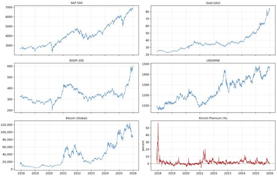
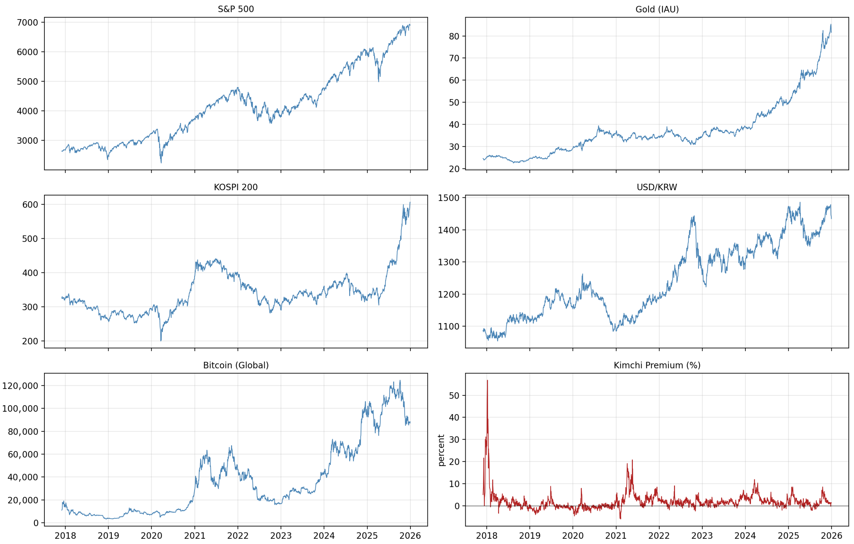
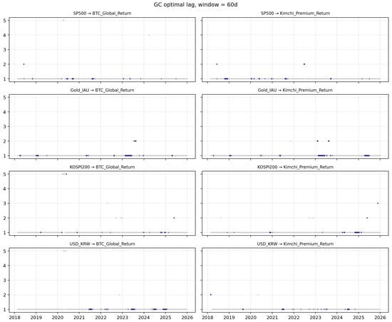
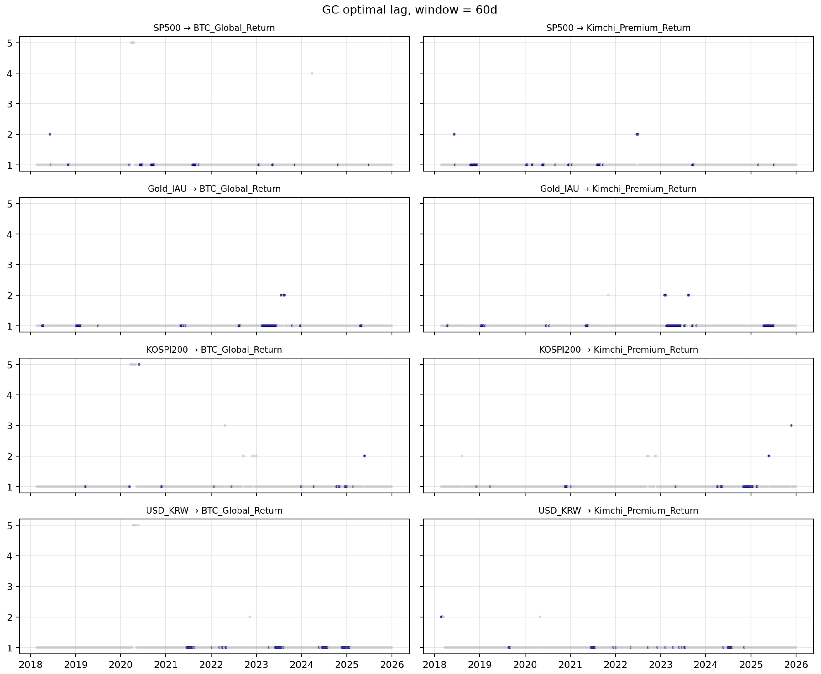
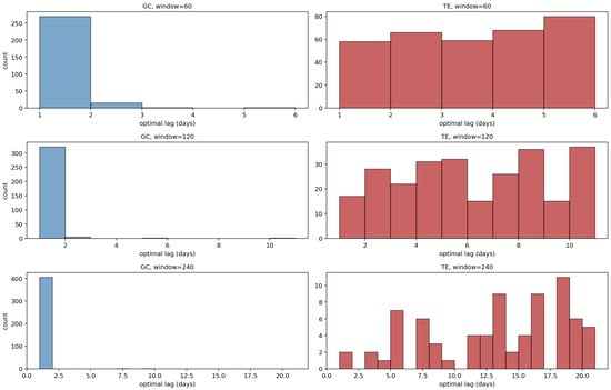
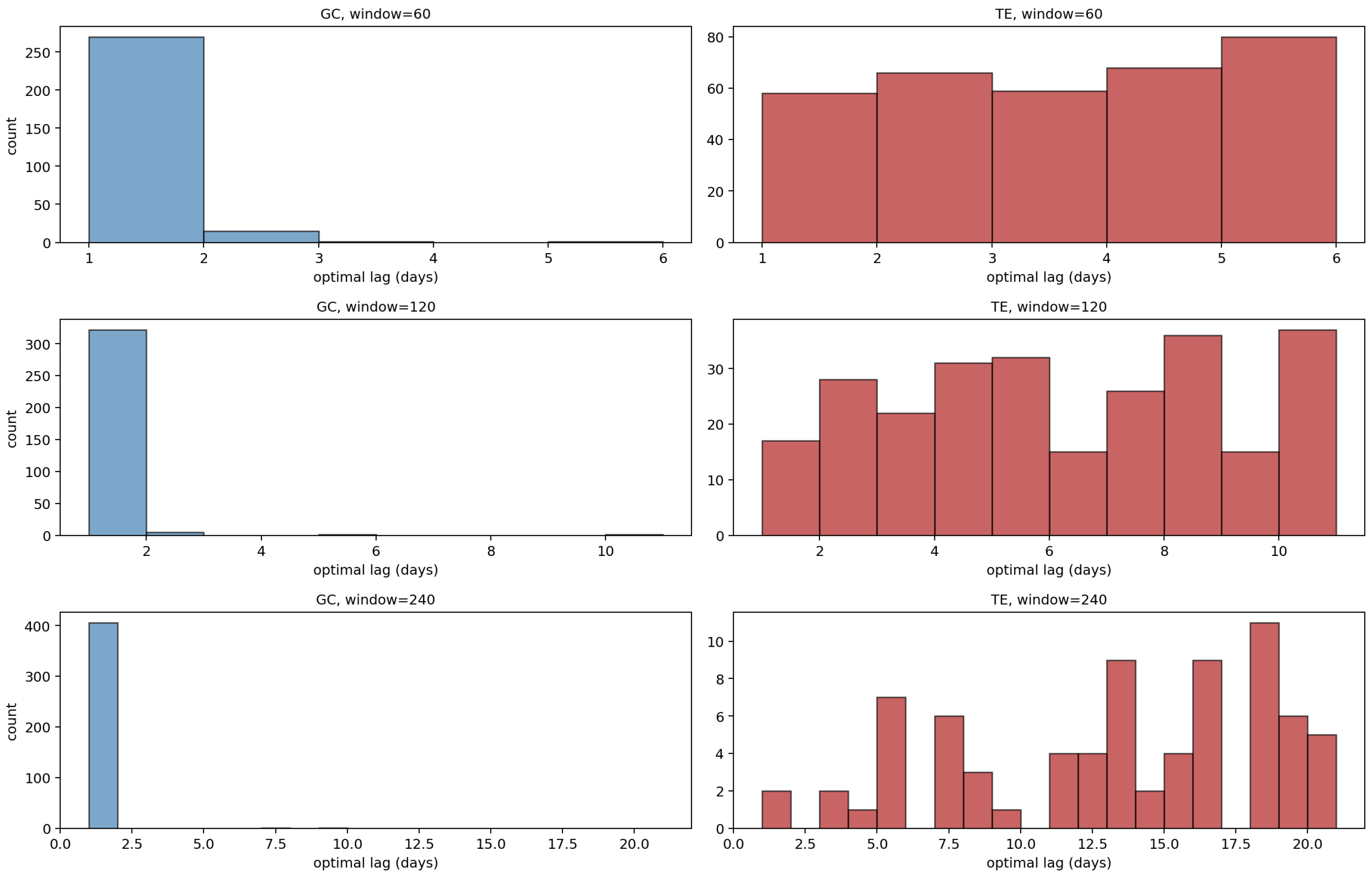
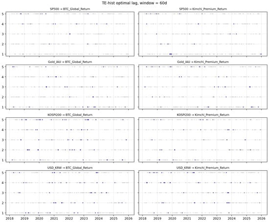
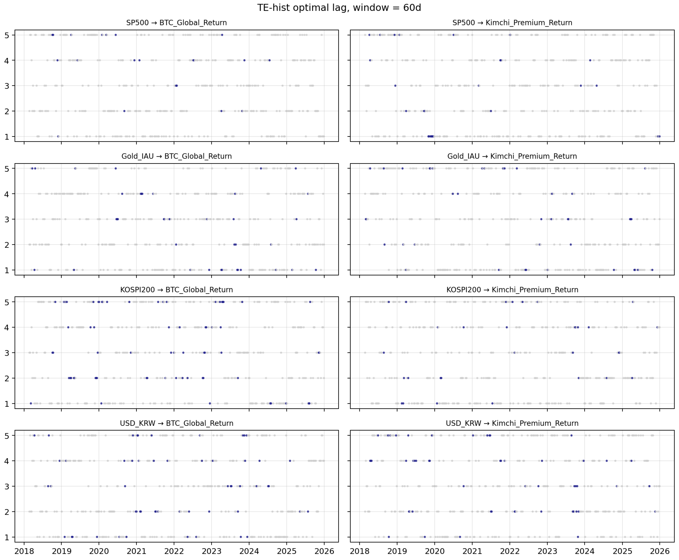
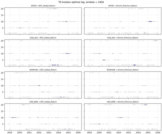
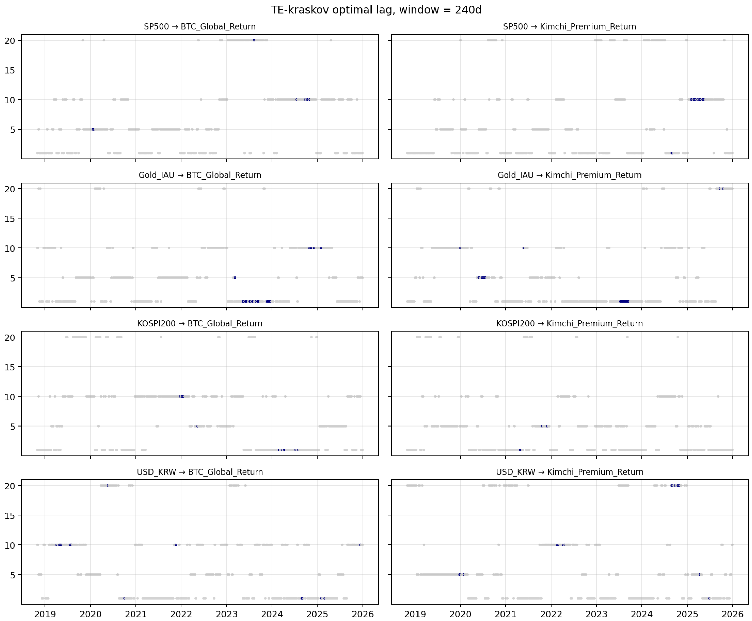
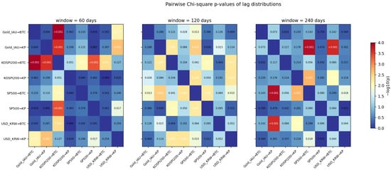
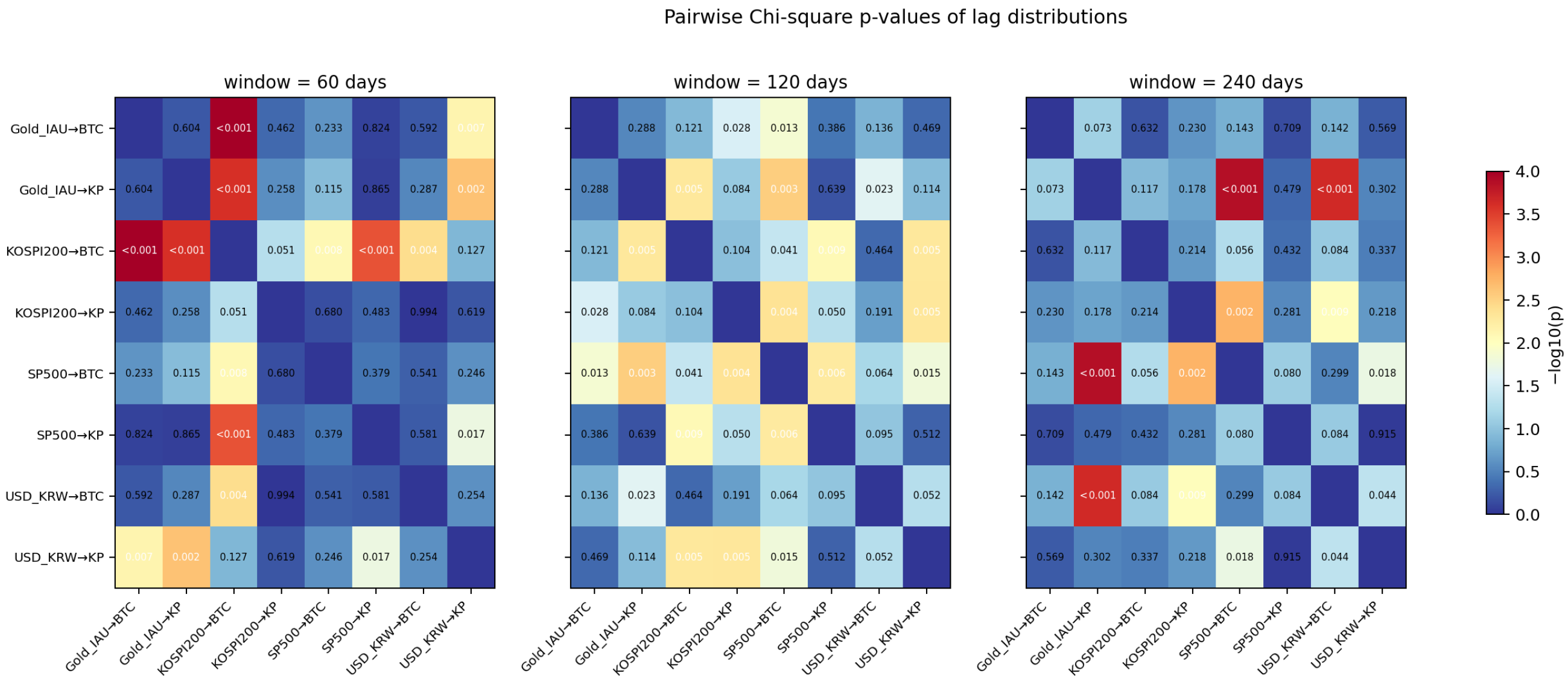
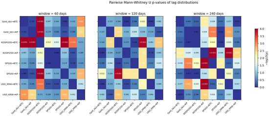
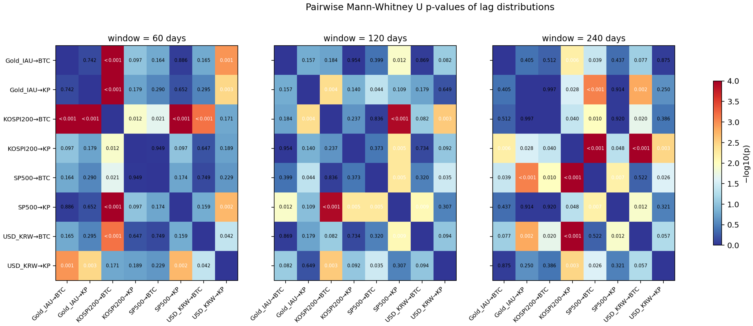

Disclaimer/Publisher’s Note: The statements, opinions and data contained in all publications are solely those of the individual author(s) and contributor(s) and not of MDPI and/or the editor(s). MDPI and/or the editor(s) disclaim responsibility for any injury to people or property resulting from any ideas, methods, instructions or products referred to in the content. |
© 2026 by the author. Licensee MDPI, Basel, Switzerland. This article is an open access article distributed under the terms and conditions of the Creative Commons Attribution (CC BY) license.