


Abstract
Software-defined networking (SDN) represents a paradigm shift in network management, but its centralized control plane introduces new and severe security vulnerabilities. Conventional intrusion detection systems, including signature- and rule-based methods, lack adaptability and interpretability in the face of evolving threats. This paper proposes a multi-hybrid deep learning fusion ensemble (MHDLFE) to enhance intrusion detection in SDN environments. The framework integrates Deep Neural Networks (DNNs), Convolutional Neural Networks (CNNs), Recurrent Neural Networks (RNNs), and Long Short-Term Memory (LSTM) models via feature fusion and a meta-classifier, thereby improving both detection performance and robustness. To address the critical need for transparency in security systems, the proposed approach incorporates Explainable AI techniques, specifically Shapley Additive Explanations (SHAP) and Local Interpretable Model-agnostic Explanations (LIME), providing interpretable insights into model decisions. The proposed model achieves strong performance on the NSL-KDD and CIC-IDS2017 datasets, attaining near-perfect binary classification scores of 97.91% and 93.30%, and multiclass accuracies of 98.61% and 97.91%, respectively. These results demonstrate that the proposed framework delivers an effective and trustworthy SDN intrusion detection system by combining deep learning, ensemble fusion, and explainable AI to support accurate, transparent, and reliable cybersecurity decision-making.
Keywords:
deep learning; ensemble fusion; explainable AI; intrusion detection; SHAP; LIME; neural network; software-defined networking MSC:
68T07; 62M10
1. Introduction
Computer networks have become an integral part of our lives. The growth of the Internet is accelerating rapidly [1]. Systems connected to the Internet face various security risks. The diversity of the Internet has grown over time, and with it, the variety of threats and vulnerabilities has grown in quantity and complexity. AI has resolved numerous real-world issues [2]. If used properly, Artificial Intelligence (AI) can help overcome these problems. In many ways, it has advanced significantly. Deep Learning (DL) and Machine Learning (ML) are examples of this development. Reinforcement Learning (RL) is widely used, with applications in robotics, cloud computing, finance, healthcare, smart cities, electric grid stations, and e-learning [3]. In RL, agents decide sequentially based on context. It makes independent decisions as it learns. Throughout the procedure, the agent follows the feedback. It works best when decisions are made sequentially, and actions lead to environmental exploration in search of the optimal model. The Internet is vulnerable to cyberattacks. Modern technologies complement each other in many ways. Owing to its constant evolution, security has drawn much attention over the past several years. Due to bandwidth growth, more complex security concerns have emerged. This study aims to develop a strategy to enhance a network’s security against malicious Internet traffic [4].
One way to protect the SDN network controller is to use a Network Intrusion Detection and Prevention System (NIDPS). The NIDPS serves as a security shield, monitoring the network 24/7 for suspicious activity that could constitute an attack [5]. There are different kinds of protection systems, and one common approach is called “signature-based.” This type of protection mainly relies on a list of well-known, previously identified attack patterns. The attack patterns are similar to how antivirus software uses its updated database of attack signatures to identify a virus. The protection database must be updated regularly with the latest attack patterns to ensure effective operation. Protecting the SDN network controller is critical. This is because the controller works as the control center, and the entire network goes down if it is hacked. In this scenario, a protection system keeps it safe and monitors network traffic for suspicious activities or attacks [6].
Various intrusion detection systems (IDSs) [7] have been developed to detect attacks in software-defined networks (SDNs) and similar systems. The current study distinguishes itself from previous studies through several new contributions. Current solutions are often characterized by limited flexibility to new threats, reliance on outdated data, and a lack of interpretability, thereby undermining their usefulness in dealing with dynamic networks. The present research attempts to reduce these shortcomings through a sophisticated approach that combines disparate classifiers into a hybrid ensemble model and, in a synergistic manner, increases its ability to detect and overall strength.
In addition, the research uses modern datasets, such as the NSL-KDD benchmark and the CIC-IDS2017 repository, which are specifically designed to reflect modern network traffic patterns and attack techniques. The choice of this model makes it particularly relevant and efficient in addressing current security challenges. By incorporating Explainable AI (XAI) systems, the level of interpretability of the model predictions is enhanced significantly by providing useful information about the decision-making process [8].
Therefore, this research makes a major contribution to the methodological and practical relevance of using IDS in changing network environments.
1.1. Software-Defined Networking and Its Relevance
Knowledge-Defined Networking (KDN) is considered an extension of Software-Defined Networking (SDN) that adds machine learning (ML) and artificial intelligence (AI) algorithms to build adaptive self-learning network systems. Unlike traditional SDN, where the data and control planes are demarcated, KDN introduces an additional knowledge plane that derives actionable insights from data aggregated by the management plane. These lessons are then used to optimize network operations, improve security, and dynamically respond to changing network conditions [9].
The KDN knowledge plane uses ML models to perform functions such as intrusion detection, traffic classification, and routing optimization. The models analyze network traffic data to develop knowledge-based rules and policies, which are then disseminated and implemented across different planes. The paradigm supports automated, context-aware decision-making, which can dramatically improve network efficiency and security [9].
The proposed MHDLFE model fits perfectly into the Knowledge-Defined Networking (KDN) paradigm. It uses machine learning to pull actionable knowledge from network traffic patterns and deliver clear, interpretable intrusion detection decisions. By adding Explainable AI tools such as SHAP and LIME, MHDLFE improves detection accuracy. This integration ensures transparent reasoning, making it a strong, reliable choice for KDN-powered intrusion detection systems.
1.2. Main Contributions
The MHDLFE framework enables ensemble-based intrusion detection by enabling three key improvements: higher detection accuracy, greater adaptability to evolving threats, and stronger interpretability.
- Heterogeneous Architecture Integration: The framework combines four different types of deep neural networks that excel in specific areas. The strengths are: Deep Neural Networks (DNNs) for abstract pattern recognition; Convolutional Neural Networks (CNNs) for spatial feature recognition; Recurrent Neural Networks (RNNs) for short-term sequence recognition; and Long Short-Term Memory (LSTM) for long-term temporal dependencies. The multiple-view approach can capture all aspects of network traffic, whereas any single model cannot. It is tested on two large datasets of attack data (NSL-KDD, CIC-IDS2017) using a stratified split to ensure accurate, generalizable results.
- LSTM-based Meta-Classification: Unlike traditional methods such as voting or averaging, MHDLFE uses an LSTM-based meta-classifier to classify the fused feature space that has 512 dimensions. This allows MHDLFE to accurately recognize and classify various types of attacks with complex, time-varying characteristics (e.g., brute-force, SQL injection, DDoS).
- Integrating Explainability: To make MHDLFE decision-making processes more transparent, explainable, and aligned with real-world requirements, SHAP and LIME are integrated for both global and local explanations.
1.3. Paper Organization
The remainder of this paper is structured as follows: Section 2 reviews the related work. Section 3 presents the datasets and preprocessing pipeline. Section 4 and Section 5 describe the proposed method and experimental setup. Section 6 presents the experimental results. Finally, Section 7 concludes the paper.
2. Background and Related Work
This section provides an overview of the current approaches to SDN security, with a particular focus on Network Intrusion Detection and Prevention Systems (NIDPSs) and emerging machine learning techniques for threat detection.
2.1. SDN Security and Network Intrusion Detection
As with many other paradigms of computer networking, Software-Defined Networks (SDNs) raise multiple new security concerns due to their single, centralized point of control. The point of control in SDNs is called an SDN controller, and because it manages and communicates with all other elements across the entire network, it is a prime focus for malicious actors [10]. These systems protect SDN controllers at the expense of other network functionalities by detecting active intrusions in real time by analyzing network traffic to match predefined attack signatures.
SDN architectures are centralized computer networking systems and, by design, are more vulnerable to, for instance, Distributed Denial of Service (DDoS) attacks, in which an SDN controller can be incapacitated by flooding it with requests, rendering it non-operational and disrupting the entire SDN. Various techniques have been developed to handle such scenarios in computer networking [11].
2.2. Machine Learning Approaches for Intrusion Detection
Recent advances in machine learning have significantly enhanced intrusion detection capabilities. Deep learning techniques, including Convolutional Neural Networks (CNNs), Recurrent Neural Networks (RNNs), Generative Adversarial Networks (GANs), and Multilayer Perceptrons (MLPs), have been successfully applied to network security applications. Notably, hybrid CNN-based models utilizing SD-Reg regularization have demonstrated superior performance in detecting both known and unknown attack patterns compared with conventional approaches [12].
Autonomous learning models that continuously adapt to the ever-changing challenges of botnet detection have been documented [13]. These systems greatly enhance the ability to detect complex network environments autonomously.
Deep learning models in intrusion detection systems rest heavily on feature selection. Transformer models achieved 99.02% accuracy, whereas CNN-LSTM models achieved 99.19% accuracy with only six selected features [14]. It shows that feature engineering is of utmost importance.
2.3. Attention-Based Intrusion Detection Systems
One advantage of using attention mechanisms in IDS is that they can direct processing resources toward the most important aspects of network traffic. The use of LSTM architectures in combination with an attention mechanism has been shown to improve detection by recognizing key patterns in network traffic, and improving accuracy and decreasing false negatives [15].
A hybrid model combining BiGRU with attention and Inception CNNs has been demonstrated to be a viable alternative. The hybrid model leverages the strengths of all three components to achieve robust attack detection and consistent detection across different types of network traffic [16].
2.4. Federated Learning for Privacy-Preserving Intrusion Detection
The privacy concerns of traditional centralized IDS have led to the emergence of Federated Learning (FL), a paradigm for Collaborative IDS [17]. Federated IDS enables multiple Organizations or Devices to Train Detection Models Jointly. Without Sharing Raw Sensitive Data, FL Preserves Privacy While Utilizing Collective Knowledge.
The latest examples of applying federated learning to vehicular IoT networks have proven successful [18]. In such networks, distributed edge devices can contribute to training a global model while still ensuring data privacy, data locality, and low communication overhead. FL-based IDS has been reviewed and analyzed recently, and while the promise of this approach is clear, there are issues with model aggregation, communication efficiency, and the problem posed by non-identically distributed data [19,20].
2.5. Explainable AI in Network Security
The need for interpretable security decisions has spurred interest in incorporating Explainable Artificial Intelligence (XAI) methods into the network intrusion detection domain [21]. For instance, understanding an AI system’s reasoning is critical in IoT networks, and the ability to explain and justify case decisions, coupled with the ability to learn system behaviors, facilitates the trust required for automated detection systems. Overall, the technology achieves its objective if the system user (e.g., a security analyst) can trust the system and make decisions based on the provided explanation and justification [22].
However, implementing XAI in network intrusion detection faces several challenges. These systems may be susceptible to higher false-positive rates, potentially misclassifying legitimate system behaviors as anomalous activity, thereby affecting overall detection accuracy.
2.6. Research Gaps and Motivation
Despite ongoing studies on SDN security, gaps remain. Many studies focus on a single type of attack or machine learning, often overlooking the rest of the security ecosystem. Other studies continue to look at the integration of multiple detection mechanisms, evolving attack patterns, and the trade-off between detection accuracy and efficiency.
Centralized SDN enables network management from a single location. However, SDN’s unique architecture presents security challenges, including the need for new mitigation strategies and adaptable detection and defense mechanisms. This research addresses these challenges by presenting a new framework that integrates cutting-edge machine learning with network management to enhance SDN controls against advanced DDoS attacks.
2.7. Deep Learning Models Overview
To address the limitations of traditional IDS approaches, this study leverages multiple deep learning architectures. Understanding the mathematical foundations of these models is essential for comprehending the proposed fusion approach. The following subsections detail the core architectures employed in the MHDLFE.
2.7.1. Deep Neural Network (DNN)
A DNN consists of multiple layers of neurons [23]. Each layer performs a linear transformation followed by a nonlinear activation function, as shown in Equation (1). Mathematically, for a given layer s
where
- is the processed output at stage s;
- is the transformation matrix associated with stage s;
- is the shift term (bias) for stage s;
- is a non-linear activation like sigmoid, tanh, or ReLU.
2.7.2. Convolutional Neural Networks (CNNs)
CNNs use convolutional layers, as shown in Equation (2) to extract spatial features from the input data [24]. The operation is defined as follows:
where
- is the transformed value at spatial location in the r-th output channel;
- denotes the transformation kernel’s parameter at index for input channel d and output channel r;
- is the input feature at adjusted location within channel d;
- is the bias associated with the r-th output channel;
- is a non-linear activation function (ReLU or sigmoid).
2.7.3. Recurrent Neural Networks (RNNs)
RNNs process sequences, as shown in Equation (3), by maintaining a hidden state that captures information from previous time steps [25]. The update rule for the hidden state is as follows:
where
- is the latent state at time index t;
- is the transformation matrix associated with prior states;
- is the transformation matrix linked to the new input ;
- is the bias term;
- is a non-linear activation function, such as sigmoid, tanh, or ReLU.
2.7.4. Long Short-Term Memory (LSTM)
The LSTM network uses special units called memory cells to store information [26]. Memory cells are controlled by gates that regulate the flow of information, as shown in Equation (4). The equations are:
3. Dataset & Preprocessing
This section focuses on IoT-specific data challenges and details our curated datasets (NSL-KDD and CIC-IDS2017) and specialized preprocessing to address data heterogeneity and imbalance.
3.1. Dataset Selection and Characteristics
NSL-KDD Dataset: NSL-KDD was built as an expanded edition of the KDD Cup 1999 dataset to support IDS testing. The most significant expansion of this new dataset compared with its precursor is the elimination of all redundant or duplicate data that were included in the KDD Cup 1999. This allows for a dataset that is more filtered, balanced, and realistic for model training and testing. The dataset contains many different types of network traffic, each of which must be classified as either normal or an attack. The attack types can be further categorized into 4 major classes: Denial-of-Service (DoS) attacks, Remote-to-Local (R2L) attacks, User-to-Root (U2R) attacks, and probing attacks. For researchers designing effective and robust IDSs, the NSL-KDD dataset is a must-have resource [27].
CIC-IDS2017 Dataset: One of the new datasets for network intrusion detection is the CIC-IDS2017 dataset. The data is from the Canadian Institute for Cybersecurity and aims to provide some of the upcoming challenges facing modern-day cybersecurity. The CIC-IDS2017 is one of the more distinctive datasets because it includes data from IoT networks. The datasets from CIC-IDS2017 include data for the following protocols: HTTP, FTP, SSH, and email, as well as the upcoming challenges facing modern-day HTTPS. Overall, the CIC-IDS2017 dataset is useful for enhancing Network Intrusion Detection systems [28].
3.2. Data Preprocessing
The following preprocessing steps were applied in strict sequential order for both datasets:
- 1.
- Handling Missing Values: NSL-KDD uses mean/median imputation; CIC-IDS2017 uses forward/backward filling.
- 2.
- Removing Duplicates: Duplicate records eliminated from both datasets.
- 3.
- Outlier Removal: NSL-KDD uses z-score (); CIC-IDS2017 uses IQR-based filtering.
- 4.
- Categorical Encoding: One-hot and label encoding were applied to convert categorical variables to a numerical format.
- 5.
- Normalization: Min-max scaling followed by z-score normalization applied to all features.
- 6.
- Class Imbalance Handling: SMOTE applied to NSL-KDD; SMOTE or ADASYN applied to CIC-IDS2017, followed by majority class undersampling for both datasets.
- 7.
- Train/Validation/Test Splitting: Stratified sampling into 70% training, 10% validation, and 20% testing subsets.
We applied the preprocessing steps shown in Figure 1 and in Table 1 to the NSL-KDD and CIC-IDS2017 datasets to make them model-ready for the DL process. The data were cleaned by imputing missing values: NSL-KDD uses mean or median imputation, whereas CIC-IDS2017 employs forward or backward filling. Then, duplicate records from both datasets were removed, and outliers in the NSL-KDD dataset were identified using the z-score method. In contrast, the CIC-IDS2017 dataset was filtered based on the Interquartile Range (IQR).
Figure 1.
Data preprocessing flow chart.
Table 1.
Dataset Preprocessing for NSL-KDD and CIC-IDS2017.
This was followed by normalization, specifically min-max scaling, which maps the features to the [0, 1] range. Z-Score Normalization was performed to scale the features to a mean of zero and a variance of one. We used one-hot and label encoding on both datasets to handle categorical variables, converting them to numerical formats suitable for model training.
Given the class imbalance, SMOTE oversampling was applied to the NSL-KDD dataset. On the other hand, CIC-IDS2017 uses either SMOTE or ADASYN processes to oversample the minority classes. For both datasets, undersampling was also employed to reduce the majority class and balance the class distributions. Stratified sampling was then used to divide the data into three segments 70% for training, 10% for validation, and 20% for testing, while maintaining the class proportions across all segments.
4. Proposed Methodology
The MHDLFE framework offers a new approach to addressing the challenges of Network Intrusion Detection and Prevention Systems (NIDPS) in Software-Defined Networking (SDN) environments. MHDLFE leverages the unique advantages of several deep learning frameworks, specifically Deep Neural Networks (DNNs), Convolutional Neural Networks (CNNs), Recurrent Neural Networks (RNNs), and Long Short-Term Memory (LSTM) Networks, as shown in Figure 2. The framework develops a range of base classifiers, new optimal activation functions, and novel ensemble strategies to address model heterogeneity, as shown in Figure 3. Also, some methods from Explainable AI (XAI), particularly SHAP and LIME, improve model explainability by providing more transparent decision-making, increasing trust, and aiding the debugging of anomalies in security-related systems.
Figure 2.
The proposed framework of the MHDLFE for SDN network systems, comprising four base models (DNN, CNN, RNN, LSTM) for feature extraction, a feature fusion module producing a 512-dimensional vector, and an LSTM meta-classifier for final intrusion prediction.
Figure 3.
The proposed model architecture of the MHDLFE for SDN network systems.
In the proposed MHDLFE, ensemble refers to a stacking-based strategy in which four independently trained base models (DNN, CNN, RNN, LSTM) extract complementary feature representations; their fused outputs are processed by an LSTM meta-classifier for final prediction, unlike traditional voting or averaging-based ensemble methods.
4.1. System Architecture and Feature Fusion Strategy
Raw input to all base models consists of normalized numerical feature matrices of shape , where n is the number of samples and d is the number of features (41 for NSL-KDD; 78 for CIC-IDS2017). Although deep learning does not require manual feature extraction, each base model learns latent representations from its final layer:
- DNN: Final dense layer →.
- CNN: Global Average Pooling →.
- RNN: Final hidden state →.
- LSTM: Memory cell output →.
These are fused via weighted concatenation into a unified vector, as detailed in Table 2. Although deep learning does not require manual feature extraction, each base model learns latent representations from its final layer-DNN (dense layer, ), CNN (Global Average Pooling, ), RNN (hidden state, ), and LSTM (memory cell output, )—fused via concatenation:
Table 2.
Base Model Architectures and Meta-Classifier Specifications.
4.2. Meta-Classification Architecture
The fused feature vector serves as input to an LSTM-based meta-classifier, which processes the concatenated features in a sequential architecture (Algorithm 1). The fused feature vector of dimension is reshaped to before being fed into the LSTM meta-classifier, enabling sequential processing of the fused representations. The meta-classifier comprises the following:
- LSTM layers: Model temporal dynamics across the fused feature space.
- Dense layers with ReLU activation: Introduce non-linearity and enhance learning capacity.
- Dropout regularization: Prevents overfitting and improves generalization to unseen network traffic patterns.
- Sigmoid output layer: Generates probabilistic intrusion predictions.
This design choice leverages the sequential nature of network intrusion patterns, thereby enabling the detection of time-dependent anomalies that traditional ensemble methods might overlook.
| Algorithm 1 Proposed Multi-hybrid Deep Learning Fusion Ensemble (MHDLFE) |
|
4.3. Framework Capabilities and Integration
The MHDLFE framework addresses several critical aspects of modern network security.
- SDN-Specific Security: Targets vulnerabilities inherent to SDN’s centralized control architecture, addressing novel attack vectors that exploit centralized network management.
- Adaptive Threat Detection: Network anomaly detection (both general and specific) and the detection of various types of cyber-attacks (e.g., DDoS, SQL Injection, and Brute-Force) are enabled by its Hybrid Deep Learning Architecture, which evolves to adapt to changing threats.
- Explainable Decision-Making: The addition of SHAP and LIME enables the system to provide an understandable explanation for why a decision was made. This addresses one of the major challenges in using deep learning models for high-stakes applications like cybersecurity. (i.e., “Black Box” problem.)
- Superior Performance: Achieves high accuracy in both binary and multiclass classification tasks, demonstrating effectiveness across various network conditions and attack scenarios.
This method provides solid, reliable, and clear intrusion detection tailored to the shifting security needs of SDN environments.
5. Experimental Setup
In this section, we describe the evaluation framework and technical architecture used to assess the performance of our proposed IDS. Our experimental design was intended to be reproducible, and we evaluated the IDS’s performance from multiple angles using various performance measures.
5.1. Evaluation Metrics
After carefully categorizing data points, conventional measures like accuracy,
F1 score,
and classification reports,
The ROC curve was used to evaluate the overall performance.
This step provides valuable information on the performance of each model in several classes [29]. The K-fold cross-validation method was employed to evaluate the consistency and performance of the classifiers in terms of accuracy across different training data splits.
In our setup, . For each fold, the model is trained on segments and tested on the remaining one.
We also plotted the learning curves to track the performance changes as the training data size increased, helping to identify overfitting or underfitting and determine the ideal training set size.
where L is the loss function, n is the number of training samples, and m is the number of validation samples.
The proposed architecture was analyzed using the “Netron” [30] tool to verify layer configurations and connectivity, with key architectural details summarized in Table 2.
In Algorithm 2, the procedure generates the history dataframe for use with the training and validation metrics (e.g., loss and precision) over a specified number of epochs. The algorithm initializes an empty history object and iteratively trains a model on the training dataset, tests the trained model on the validation dataset, and stores the test results in the history object. Other metrics are available in the history object to enable further analysis.
| Algorithm 2 History Data Frame Creation for Model Training |
| Require: Training data , Validation data , Number of epochs Ensure: the History data frame contains training and validation metrics |
|
Algorithm 3 enables visualization of how training and validation performance may change over epochs. It organizes the historical data into a DataFrame and uses the Seaborn-0.13.2 library to generate line plots for each performance metric, such as accuracy or loss, over the specified number of epochs. Visualizing performance metrics allows assessing the model’s performance across training epochs and helps identify overfitting and underfitting.
| Algorithm 3 Plot Training Progress for Deep Learning Model |
| Require: Training history dictionary H containing loss and accuracy metrics Ensure: Line plots for training progress |
|
Algorithm 4 provides a complete process of training the model and visualizing its performance in a single workflow. At first, it trains the LSTM model, records and organizes the training metrics systematically, so as to facilitate further analysis. Using Seaborn, we obtain a separate figure for each evaluation metric, which helps us better assess how this model converges and remains stable. In addition, the aforementioned algorithms provide an integrated approach for easily fine-tuning hyperparameters and improving the model. Furthermore, the presented algorithms offer a reproducible deep learning pipeline that increases the analytical precision and interpretability.
| Algorithm 4 Training LSTM Model and Plotting Training History |
| Require: (Training data), (Training labels) Ensure: Training history as a DataFrame, Performance visualization |
|
Figure 4 and Figure 5 depict the evolution of the training procedure of the proposed MHDLFE in the context of binary and multi-class classifications. In both contexts, the training and validation losses evolve smoothly and progressively over the training epochs, and convergence is reached at values close to optimal. Therefore, the proposed methodology achieves a good trade-off between learning and overfitting. Moreover, the small difference between the training and validation curves indicates that the proposed methodology has a strong ability to generalize across both types of classification problems.
Figure 4.
Training progress of a binary-class DL model across epochs. Each dot represents the metric value at a single epoch; the line denotes the overall trend, and the shaded region indicates the 95% confidence interval.
Figure 5.
Training progress of a multiclass DL model across epochs. Each dot represents the metric value at a single epoch, connected sequentially to illustrate per-epoch fluctuations in loss and accuracy.
5.2. Hardware & Software Configuration
We used Python version 3.12.2, an open-source environment, along with several other open-source libraries, including pandas, scikit-learn, and seaborn. These libraries are useful for reading and manipulating input data with pandas; for performing all aspects of machine learning (i.e., data splitting, model training, model evaluation) with scikit-learn; and for displaying results from model runs with seaborn. The system was run on a 2.2 GHz Intel Core i5-8th Gen processor, with 32 GB of memory, and with a 2 GB AMD Radeon video card. We selected the most appropriate Python modules to perform model training and evaluation. The main steps in the process were preparing the data, training the model, evaluating its performance, and visualizing the results; as a result, we were able to clearly communicate the model’s capabilities.
5.3. Reproducibility
To ensure the reproducibility of the results:
- All random seeds are fixed and documented.
- Detailed hyperparameter settings are provided.
- Dataset preprocessing steps are fully specified.
5.4. Training, Validation, and Testing Protocol
The base models (DNNs, CNNs, RNNs, and LSTMs), as well as the LSTM meta-classifier, were each trained in succession on identical data partitions, ensuring a comparable basis for comparison. The two datasets were split stratified into 70% training, 10% validation, and 20% test sets, preserving the class distribution across all splits and applying it uniformly to all models. A single base model was trained independently; after which the fused output features from this model were used to train the same process and the meta-classifier. In addition, k-fold cross-validation () was used in the ablation study, where, during training, of the data was used for training, and was used for validation in each fold; then the average of the metrics over the folds was computed to provide a more robust assessment of the performance.
6. Results and Discussion
MHDLFE emphasizes the importance of interpretability in modeling through visualization. Advanced 3D visualization tools are used to illustrate the complexity of relationships within the data and to assist users in visualizing the architecture of DL models, such as Netron. Visualization of feature maps also allows researchers to see how DL models handle loss and accuracy over time, as shown in Figure 4 and Figure 5 at every epoch. In addition, the activation of neuron-layer combinations can further illustrate how information is being processed throughout the network. These comprehensive visualization approaches allow researchers to gain valuable insights about how decisions were made.
6.1. Confusion Matrix Binary and Multiclass
The proposed MHDLEF model performs well on binary classification metrics on the NSL-KDD dataset, as shown in Figure 6. For Class 0, 19,871 instances were predicted correctly, but 212 were misclassified as Class 1. Class 1 had 17,134 correct predictions, with 575 cases misclassified as Class 0.
Figure 6.
Confusion matrices for the proposed model on the NSL-KDD dataset, for binary classification.
The confusion matrices for the DNN, CNN, RNN, and LSTM models show detailed performance metrics for each class. For class 0, 6649 instances were correctly predicted, but 12 instances were misclassified as class 1, 19 as class 2, and 17 as class 3. Class 1 had 4603 correct predictions, with 7 instances misclassified as class 0. Class 2 had 1170 correct predictions, but 12 instances were misclassified as class 0. Class 3 had 90 correct predictions, with 10 misclassifications of Class 0. Class 4 had 2 correct predictions and 5 instances misclassified as class 0. For the CNN, 6638 class 0 instances were correctly predicted, but 7 were misclassified as class 1, 16 as class 2, and 36 as class 3. Class 1 had 4602 correct predictions, with eight instances misclassified as class 0. Class 2 had 1170 correct predictions, but 11 instances were misclassified as class 0, 1 as class 1, and 1 as class 3. Class 3 had 92 correct predictions, with eight instances misclassified as class 0. Class 4 had two correct predictions, with four instances misclassified as class 0 and one as class 3.
The proposed MHDLEF model performs well on multiclass metrics, as shown in Figure 7. As usual, 1333 instances were correctly predicted, but one was misclassified as class 1, one as class 2, and 0 as classes 3 and 4. Class 1 (dos) had 932 correct predictions, with three instances misclassified as class 0 and 0 for classes 2, 3, and 4. Class 2 (probe) had 221 correct predictions, but two cases were misclassified as class 0 and three as class 1. Additionally, Class 3 (r2l) predicted zero instances correctly while misclassifying one instance as class 0, three instances as class 1, and 19 instances as class 2. Class 4 (u2r): One instance was predicted as a misclassification of class 2.
Figure 7.
Confusion matrices for the proposed model on the NSL-KDD dataset for multiclass classification.
The proposed MHDLEF model also performs well on binary and multiclass classification metrics using the CIC-IDS2017 dataset, as shown in Figure 8. The model performs excellently in binary classification, correctly classifying 1776 normal and 1829 malicious instances. However, it misclassifies 137 normal instances as malicious, yielding 137 false positives (FPs), and misclassifies 110 malicious instances as normal, yielding 110 false negatives (FNs). This relatively low rate of false positives (FPs) and false negatives (FNs) suggests that the model performs well at discriminating between normal and malicious traffic. However, there is still room to reduce misclassifications further.
Figure 8.
Confusion matrices for the proposed model on the CIC-IDS2017 dataset, for binary and multiclass classification.
The performance of the multiclass classifier varied across six categories (0–5). Class 0 is likely normal traffic and has many TPs (123,950), yet it still suffers from misclassifications into other categories; for example, 1360 were labeled as Class 1. In contrast, Class 1, which characterizes a specific attack, achieved 126,423 correct predictions but had FPs misclassified into other classes, with 486 being predicted as Class 0 and 2140 as Class 3. The breakdown of results across classes is similar, with significant false positives (FPs) and false negatives (FNs) more specific to certain attack classes, such as Class 4, where 262 instances were incorrectly classified as Classes 3 and 5.
The performance metrics of the DL models were evaluated for binary classification, as shown in Figure 6. The results prove the excellent performance of all the models. The DNN model achieved a precision of 99.43%, indicating high accuracy, recall, and F1 score. The CNN model achieved a precision of 99.21%, demonstrating balanced performance across precision and recall. The RNN and LSTM models achieved accuracies of 98.98% and 98.07%, respectively, along with recall and F1 scores of 98.98% and 98.07%, respectively. The proposed MHDLEF model demonstrated excellent performance in binary classification, achieving perfect scores across all criteria and an overall accuracy of 97.91%. These results prove the effectiveness of the proposed method for binary classifications. These results also suggest that all models were highly influential in classifying instances, indicating their robustness and suitability for binary classification tasks.
In contrast, the evaluation for multiclass classification also shows prominent performance, as shown in Figure 7. The DNN model achieved an accuracy of 88.11% and correctly classified all instances. The CNN model achieved an accuracy of 98.55%, indicating balanced performance. The RNN and LSTM models demonstrated reliable performance, achieving accuracies of 94.73% and 98.33%, respectively. The proposed MHDLEF model for multiclass classification achieved balanced precision, recall, and F1 scores of 97.76%, 98.65%, and 98.19%, respectively, which are comparable to those of the CNN model, which also yielded an accuracy of 98.55% and precision, recall, and F1 scores of 98.55%. These findings highlight the suitability of these models for addressing complex multiclass classification tasks.
6.2. ROC Curve Analysis
Figure 9 provides an overview of the ROC curves showing how the proposed Model performed on the NSL-KDD dataset for both binary and multi-class classification. Binary Classification has an AUC of 0.9971, indicating excellent discrimination between the two classes. Hence, it achieves optimal management of False Positives (FP) and maximizes True Positives (TP). Multi-Classification had AUC values ranging from 0.9012 to 0.9991. These AUC values show the Model’s ability to handle increasingly difficult classification scenarios. Overall, this demonstrates that the Model performs equally well across simple, multi-class, and binary classification tasks.
Figure 9.
ROC curves for the proposed model on the NSL-KDD dataset, binary and multiclass classification performance.
The ROC Curve in Figure 10, which was generated using binary classification for the CIC IDS 2017 data set, demonstrates an area under the curve (AUC) of 0.98. This suggests that this model will be successful at separating the malicious class from the normal class, with a high true positive (TP) rate (sensitivity) and a very low false-positive (FP) rate across the entire range of possible decision thresholds.
Figure 10.
ROC curves for the proposed model on the CIC-IDS2017 dataset, binary and multi-class classification performance.
The curve begins sharply in the top-left of the plot, indicating that the model correctly classifies most instances with only a few false positives. Each class has its own ROC curve for multiclass classification using the CIC-IDS2017 dataset. In contrast, all classes had AUCs between 0.99 and 1.00, indicating near-perfect classification performance across all categories. Conversely, Class 0, with a score of 0.99, followed the rest: Classes 1, 2, 3, and 5, all of which recorded a score of 1.00. The model performs excellently, classifying all traffic types and attacks with very few misclassifications.
6.3. Learning Curve Analysis
Figure 11 shows the learning curve analysis from the proposed model’s cross-validation process, applied to the binary and multiclass classification tasks on the NSL-KDD dataset.
Figure 11.
Learning curve analysis on our cross-validation output for binary and multiclass using NSL-KDD dataset.
The binary classifier showed a steady decline in training and validation loss. The training and validation loss of the binary classifier were extremely similar, suggesting that the model has a very low risk of overfitting. A significant increase in accuracy (near-perfect) occurred during the early epochs of the binary classifier, and training and validation accuracies reached near-perfect levels within 5 epochs. The rapid increase in the binary classifier’s accuracy further supports the notion that the model learns quickly in binary classification. In addition, a smooth decline in loss was observed for the training and validation sets of the multi-class classifier, indicating effective learning. As expected, the multi-class classifier showed significant increases in accuracy in its training and validation curves within a small number of epochs (with some minor overfitting). Although a moderate degree of overfitting was observed between the training and validation metrics for both the binary and multi-class classifiers, the model demonstrated good generalization across classification problems of varying complexity.
Figure 12 illustrates the learning curve analysis of the proposed model for both binary and multi-class classification, using the CIC-IDS2017 dataset for training and validation.
Figure 12.
Learning curve analysis on our cross-validation output for binary and multiclass using CIC-IDS2017 dataset.
The training and validation accuracies for binary classification varied over epochs, eventually stabilizing at around 90% and 92%, respectively. Following the third epoch, the validation accuracy was consistently lower than the training accuracy. This indicates that although the model performed reasonably well on the training data set, it did experience some degree of overfitting, as evidenced by the stabilization of validation accuracy in the final epochs. The training and validation loss of this model exhibited similar patterns and decreased rapidly within the first two epochs. Afterward, the training and validation loss stabilized at lower values with slight fluctuations in the validation loss.
The accuracy of training and validation for the multiclass began to increase rapidly in the first several epochs, reaching over 96% at the fourth epoch. The training and validation accuracies are closely tied, and the validation occasionally slightly outperforms the training. This indicates that the model generalizes well to the multiclass classification problem; however, the slight drop in validation accuracy in the last epoch deserves further attention. The trend is close to accuracy, indicating that training and validation losses decrease significantly in the early epochs. In most epochs, the validation loss was lower than the training loss, further confirming that the model was not overfitting and was performing well on unseen data.
Generally, all learning curves showed good training progression; however, multiclass classification performed slightly better than binary classification. It exhibited slight signs of overfitting towards the end of the binary classification. Fine-tuning or early stopping might be the solution to the overfitting observed in binary classification. Figure 9 and Figure 11 show similar trends in training and cross-validation scores for binary and multiclass classification, respectively. This trend confirms the state-of-the-art model’s ability to learn from the data, indicating that it effectively captures underlying patterns and generalizes well to new data.
6.4. Comparative Study
This section examines the performance of the proposed MHDLFE module by comparing various methods and feature algorithms. The model was evaluated against the latest ID methods to demonstrate its advantages for IDS.
6.4.1. Comparison with Classical Methods
In other model-related ablation studies, we compared our approach with existing state-of-the-art methods regarding dataset ID methodologies, as shown in Figure 13. Existing studies primarily influence datasets such as NSL-KDD by employing techniques such as LSTM AE, VAE, DCAE, and BAE [31]. Among the algorithms tested, the LSTM AE achieved an accuracy of 93.2%, with balanced precision, recall, and F1-score. The VAE and DCAE also demonstrated strong performance, with accuracies of 93.68% and 96.08% and F1 scores of 93.68% and 96.08%, respectively. In comparison, the BAE model shows slightly lower accuracy of 90.45%, with precision, recall, and F1-score of 90.47%, 90.45%, and 90.45%, respectively.
Figure 13.
Comparison with classical methods and overall performance of the proposed model architecture.
Again, our proposed binary and multiclass models, P-B and P-M, outperformed the other algorithms, achieving accuracies of 97.91% in the binary class and 98.61% in the multiclass, along with commendable precision, recall, and F1-score values of 97.7%. These results highlight the effectiveness of our proposed models in predicting targeted intrusion and demonstrate promising performance compared to other deep learning (DL) models in the study. For in-depth model analysis and performance evaluation, we also implemented a scatter plot to compare actual versus predicted performance and its impact on predictions for both binary and multiclass classification.
The scatter plot in Figure 14 illustrates multiclass classification and compares the actual labels “Before the model Implementation” with the predicted random labels from before the proposed model was implemented. We must focus on the actual and predicted data points in this plot. The class labels 0, 1, 2, 3, and 4 correspond to five classes. The Dos, Normal, Probe, U2r, and R2l were measured. Figure 15 shows the actual data points (blue) for multiclass classification, representing the accurate labels “After the model Implementation” for the samples in our test set. The ground truth was compared with our model’s predictions. The predicted data points (green) represent the labels our model assigns to the same samples. The closer these points are to the data points, the better the model’s performance.
Figure 14.
Scatter plot of actual vs. predicted labels before model implementation, where random predictions are distributed across all class labels.
Figure 15.
Scatter plot of actual vs. predicted labels after model implementation, showing strong alignment between actual and predicted classes.
6.4.2. Comparison with SOTA Methods
The accuracy achieved is comparable to that of state-of-the-art methods for dataset ID, as shown in Table 3. Existing studies primarily utilize datasets such as NSL-KDD, KDD99, CIC18, AWID, and NB15, and employ approaches such as autoencoders, ARL, CGA, and DBF. SAE, MLA, DNNs, CNNs, RNNs, and LSTMs. Notably, many of these studies utilize limited data and focus on binary classification, with only a few venturing into multiclass scenarios in specific contexts. Examining Table 3 and Figure 16 reveals that our multi-hybrid deep learning fusion ensemble-binary class (MHDLFE-B) approach achieves commendable results, achieving accuracies of 97.91% and 98.61% in multi-hybrid deep learning fusion ensemble-multiclass (MHDLFE-M), along with worthy precision, recall, and F1-score, which are 97.7% and 98.6% compared to the existing literature.
Table 3.
Comparison analysis with SOTA literature for overall accuracy performance.
Figure 16.
Surface chart for SOTA Comparison.
Our proposed MHDLFE-B and MHDLFE-M models demonstrate outstanding performance on both datasets, NSL-KDD and CIC-IDS2017, achieving accuracy of nearly 97% or higher on each. This clearly demonstrates the excellent generalization capability of our models for intrusion detection tasks. More precisely, MHDLFE-B remained at approximately 97.9% owing to its robust baseline architecture, which focuses on essential feature extraction practices. In contrast, MHDLFE-M achieves slightly higher accuracy, reaching 98.65% in some cases, indicating that the changes included in this version have paid off in its current improved performance.
Compared with existing methods, MHDLFE-B and MHDLFE-M achieve substantially higher performance than models such as CAFE-CNN and CNN-GRU, which achieve approximately 83.34% and 86.76%, respectively. While CNN architectures are very good at extracting spatial features, they seem less capable of capturing temporal dependencies that may be characteristic of cybersecurity datasets. In contrast, our models incorporate more effective strategies for handling temporal or higher-dimensional features, commensurate with the complexities of these datasets. This constitutes a significant improvement over DSSTE+CNN-miniVGGne, another hybrid model that performs well across all aspects with a score of 96.97%, yet still falls short of our models’ achievements. This may indicate that MHDLFE-B and MHDLFE-M are systems with balanced mechanisms that enhance the classification performance. A sophisticated feature-extraction pipeline or a new combination of features across different dimensions may yield further improvements.
MHDLFE has many advantages over the more common CNN-based architectures, including its ability to perform multi-layered feature extraction, enabling it to capture both local and global patterns. As a result, MHDLFE tends to perform better on complex datasets, such as CIC-IDS2017, which include a wide range of attack types. MHDLFE’s advantage also stems from its dynamic feature-extraction process. This allows it to be more flexible and handle more complex data across the two sets. In addition to the more dynamic nature of MHDLFE-M, we have optimized the architecture using more advanced data augmentation methods (such as dropout), finer-grained hyperparameter tuning, and stronger regularization. These are some of the reasons why MHDLFE-M consistently outperforms previous architectures based on NSL-KDD.
While NSL-KDD is an old and widely used dataset, MHDLFE-B and MHDLFE-M achieved extremely high performance on it (scores greater than 97.5%). MHDLFE-B and MHDLFE-M demonstrated good generalization capabilities, even on legacy datasets with less complexity than the most recent, unbalanced datasets like CIC-IDS2017. In addition, the high accuracy achieved by MHDLFE-B and MHDLFE-M on these newer, imbalanced datasets with multiple attack types demonstrates that our models effectively detected a wide variety of intrusions. Therefore, the consistent performance of MHDLFE-B and MHDLFE-M across these two very different datasets indicates that they are well-suited to a wide variety of feature spaces and data distributions. In contrast, models such as CNN-GRU or EL may not achieve the same level of versatility.
The proposed MHDLFE model achieved an average inference time of 4.1 ms per sample, demonstrating that the framework delivers efficient inference while maintaining high detection accuracy.
Our proposed models represent state-of-the-art capabilities in feature extraction and adaptation for complex and imbalanced datasets, enabling better generalization across diverse feature spaces. These attributes make the MHDLFE framework a valuable contribution to intrusion detection. In any case, applying these approaches to real-time applications and enhancing their robustness through adversarial training may open new avenues for current research.
6.5. Explainable AI
XAI frameworks, such as XAI-IDPS, are essential for network IDSs. However, with the rising significance and criticality of decisions made by AI-enabled systems, these frameworks strive to enhance the transparency of the internal black-box mechanisms within deep learning models (Figure 17) to develop trust among humans regarding AI model decisions [46,47]. SHAP [48] plots effectively show the details of feature influences, shedding light on the decision-making process of the model.
Figure 17.
XAI framework enhancing transparency of the internal black-box mechanisms within deep learning models, where SHAP and LIME provide interpretable insights into the decision-making process of the proposed MHDLFE.
In other cybersecurity domains, such as malware classification and the security of XAI methods, the transparency and interpretability of the XAI framework can be valuable. Therefore, the applications of XAI-IDS have been extended beyond network ID to various areas within cybersecurity, where the need for transparent and interpretable AI models is paramount [49].
6.5.1. SHAP Analysis
The SHAP value plot provides a breakdown of feature importance for binary and multiclass classification tasks on the NSL-KDD and CIC-IDS2017 datasets, providing interpretable insights into the model’s decision-making process.
NSL-KDD Dataset-Binary Classification (Normal vs. Attack): As shown in Figure 18a, flag dominates with the highest mean value (≈0.38), contributing nearly equally to both Class 0 and Class 1 predictions, confirming that TCP connection state is the single strongest discriminator. dst_host_same_srv_rate and logged_in follow (≈0.19 each), indicating that host-level service consistency and authentication state are jointly decisive. Notably, dst_bytes and src_bytes contribute asymmetrically, with dst_bytes exerting greater Class 0 influence, suggesting that inbound data volume is more diagnostic of normal behavior than outbound volume. The near-zero contribution of diff_srv_rate indicates service diversity alone is insufficient for binary discrimination, validating the model’s feature prioritization against domain expectations.
Figure 18.
NSL-KDD-SHAP Summary plots for binary and multiclass classification.
NSL-KDD Dataset-Multiclass Classification (Attack Types): The beeswarm plot in Figure 18b shows that the attack_flag attribute has the highest variability of SHAP values ( to ). The high values (in red) for this attribute will push the prediction towards the “attack” class, while low values (in blue) will push the prediction towards the “normal” class; therefore, it is the best multiclass discriminator. count and dst_host_diff_srv_rate have many blue dots near the origin, showing that these attributes consistently contribute to the decision of whether or not something is an attack (i.e., some positive contribution to the classification). However, occasionally there may be extreme contributions (outliers). As expected, both src_bytes and duration show red dots to the right, supporting the notion that these two attributes are used to identify high-volume and long-duration DoS attacks. The error rate attributes (serror_rate and dst_host_serror_rate), show few red dots (high values) with most dots near the origin (zero) and as expected, the red dots are sparse, which indicates that the error rate attributes are highly class specific (i.e., triggers for a particular type of attack, such as SYN flood and U2R attacks) rather than general (i.e., contributing to the classification regardless of the type of attack).
CIC-IDS2017 Dataset-Binary Classification (Normal vs. Attack): Figure 19 clearly indicates that both Bwd IAT Std (≈0.10) and Bwd IAT Total (≈0.09) were the most important factors, which indicate that irregularity and accumulation in backward inter-arrival time were the key indicators of malicious traffic. A monotonic decrease in the feature importance hierarchy, from Bwd IAT Std, down to Bwd Packet Length Mean, indicated that timing features were much more important than volume features for identifying malicious traffic. This finding contrasts with the classical signature-based IDS approach, which relies on payload size.
Figure 19.
CIC-IDS2017 -SHAP Summary plots for binary and multiclass classification.
CIC-IDS2017 Dataset-Multiclass Classification (Attack Types): The beeswarm plot shown in Figure 19b illustrates that Active Mean and Bwd Avg Packets/Bulk had the widest SHAP distribution, indicating that they are sensitive to changes in feature magnitudes regardless of attack category. Flow Packets/s exhibited a bipolar effect, where high values (red) resulted in negative SHAP contributions while low values (blue) produced positive SHAP contributions. Therefore, low packet rates may indicate certain attack types, such as slow-rate or R2U attacks. Finally, Fwd IAT Total and Source IP each exhibit sparse but large-magnitude outliers, suggesting that these two features are influenced by the specific attack type rather than being universally applicable. The dominance of flow-level and timing features over raw packet-content features across both datasets consistently supports the model’s alignment with behavioral rather than signature-based detection principles, thereby enhancing confidence in its generalizability.
Across both datasets, the SHAP analyses confirm that timing-related features, rate-based attributes, and protocol-level indicators are the most influential drivers of the model’s decisions, consistently aligning with established cybersecurity domain knowledge and reinforcing the transparency and trustworthiness of the MHDLFE framework.
6.5.2. LIME Analysis
Figure 20, Figure 21 and Figure 22 summarize these explanations at the local level by showing how the model arrives at its predictions in both binary and multiclass classification on the NSL-KDD and CIC-IDS2017 datasets, and by highlighting the most influential features. For local interpretation, we used LIME to explain the given instance, providing valuable insights into the decision-making process of the DL models. The original predicted probabilities indicated high confidence in the positive class (class 1), with a probability of 1.0 for both the binary and multiclass classifications.
Figure 20.
Local explanation of the model’s predictive probabilities for a two-class classification task using the NSL-KDD dataset.
Figure 21.
Local explanation of CIC-IDS2017 binary class performance using the CIC-IDS2017 dataset.
Figure 22.
Local explanation of CIC-IDS2017 multiclass performance using the CIC-IDS2017 dataset.
NSL-KDD Dataset (Binary Classification): As shown in Figure 20, the local explanation of the model’s predictive probabilities for a two-class classification task distinguishes between ’normal’ and ’attack’ network events. The left segment displays the model’s confidence in each class, with ’attack’ predicted with certainty. The center and right segments illustrate how various features contribute to the ’normal’ prediction, with a decision-tree breakdown and a bar chart highlighting feature values.
The “Value” field indicates the weight (or influence) of each feature on the model. For example, the value for “flag” is 0.10, indicating a significant positive influence toward a “Normal” result. In general, based on the LIME image, we have high confidence in our ability to predict whether an instance is “normal.” We can visualize the contributing features by examining the LIME image. This will allow us to see which features have the greatest influence and how each feature influences the prediction.
CIC-IDS2017 Dataset (Binary Classification): In the binary classification scenario shown in Figure 21, the model predicts a 95% probability of malicious traffic, with just a few key features driving this decision. The features that strongly contribute to the positive class are Bwd Packets/s, which denotes the packet rate in the backward direction per second, and Flow Bytes/s, which denotes the flow rate in bytes per second; high traffic rates are usually a signature of malicious activity. In addition, the destination port and Fwd IAT Min (minimum forward inter-arrival time) contributed to the model’s prediction edge towards the malicious class. While the lower values of features such as Bwd IAT Min and Flow Packets/s pull the instance towards the normal class, they are outweighed by other more influential features that support the malicious class.
CIC-IDS2017 Dataset (Multiclass Classification): Figure 22 represents the model prediction in a multiclass classification scenario to demonstrate that normal traffic is classified as Class 0 and predicted with 100% probability. The most influential features are Fwd IAT Total and Flow Packets/s, which contribute the most to predicting normal traffic. In contrast, for Class 1, which may be a specific attack type, features such as ACK Flag Count, Subflow Fwd Packets, and URG Flag Count contribute positively to its classification, indicating that packet-level and flow-related features are crucial for distinguishing different attack categories.
Therefore, features such as Bwd Avg Packets/Bulk and Bwd Packet Length Max provide additional insights into classification by identifying bulk transmission patterns in network traffic. Certain network characteristics (packet rate, inter-arrival times, flow properties) are highly important for a model’s accuracy in binary classification between normal and malicious traffic and in multiple traffic category classification. Such fine-grained information can also help understand an individual model’s decision-making and output-generation processes.
6.6. Most Influential Features in Detecting Cyber Threats
From the SHAP and LIME analyses, this study identified several key features as the most influential in detecting cyber threats:
- Timing-Related Features: Bwd IAT Std and Bwd IAT Total: If you see high variation or large values for backward inter-arrival time, there is likely no attack. However, if you observe a deviation from the standard value, it is possible to determine that an attack has occurred.
- Fwd IAT Min and Fwd IAT Total: A short or inconsistent forward inter-arrival time is typically indicative of some form of malicious activity.
- Rate-Based Features: Bwd Packets/s and Flow Packets/s: High packet rates (in either direction) are an excellent indicator that you have been attacked by a Denial-of-Service (DoS) or flooding type of attack.
- Flow Bytes/s: When the number of bytes per second within the flow exceeds a predetermined threshold, it can be a sign that you have been attacked using malicious payloads or attempting to exfiltrate your data.
- Network Flow and Packet Attributes: Destination Port Attacks may target a specific port to isolate the attack. Therefore, this could be a critical discriminator.
- ACK Flag Count and URG Flag Count: While unusual flag usage (or combinations of flags) can indicate a scan or exploit, they do not necessarily indicate an attack.
- Bwd Packet Length Max: A large maximum backward packet length may indicate that you have experienced a large volume of data being transferred related to an attack.
The set of features detects irregular patterns in traffic timing, transmission rates, and packet characteristics, which serve as indicators of cyber threats, including intrusions and malware attacks.
6.7. Improving Trust in the Model’s Decisions
The application of SHAP and LIME enhances trust in the AI model’s decisions in several ways.
- Transparency: Figure 19a,b visually demonstrate how the model uses the features of network traffic, specifically the timing and/or packet rate, to make decisions. These are two well-established indicators of an attack used by cybersecurity experts.
- The local explanations provided by LIME (Figure 20, Figure 21 and Figure 22) provide insight into each prediction and show how each decision is made. A user can see how a particular instance was labeled as either malicious or normal and how it was determined. For example, if Bwd Packets/s drove a particular prediction of a malicious connection, the user can immediately correlate it with real-world attack signatures.
- Interpretability: By quantifying how much each feature contributes to the final model output (i.e., SHAP values or LIME weights), the user can be assured that the model is not making decisions based on spurious relationships or unnecessary information. For example, the fact that the model places greater emphasis on Bwd IAT Std than on other, less relevant features (such as the actual packet payload) increases confidence in the model’s logic.
- Actionable Insights: Cybersecurity professionals can narrow the scope of their monitoring to the metrics most important to them, such as Flow Bytes/s and Destination Port. In doing so, they ensure the AI-driven decision-making process aligns with their organization’s operational needs. As such, an additional level of trust is created through actionable insights.
- Validation Against Expectations: When both SHAP/LIME outputs align with a cybersecurity professional’s expectations (for example, high packet rates indicating an attack), this adds credibility to the reasoning behind the model’s decision. If the model identifies traffic as malicious based on Bwd Packets/s and LIME shows that this decision aligns with a known attack signature, the user will be more likely to trust the model’s decision.
In this study, SHAP and LIME illuminate the black box of ML-based intrusion detection by pinpointing timing (Bwd IAT Std, Fwd IAT Min), rate (Bwd Packets/s, Flow Bytes/s), and packet/flow features (Destination Port, ACK Flag Count) as critical factors for cyber threat detection. This transparency demystifies the model’s decisions and aligns them with cybersecurity principles, thereby boosting human trust.
6.8. Discussion
6.8.1. Model Architecture and Explainability Framework
Our solution combines three other architectures: Deep Neural Networks (DNNs), Convolutional Neural Networks (CNNs), and Long Short-Term Memory (LSTM) networks. The CNN architecture includes three different layer configurations for convolutional layers and global average pooling. This is done so that each layer captures the hierarchical nature of the data’s spatial features. The LSTM architecture includes two layers, both of which use dropout regularization. The purpose of this is to learn the temporal dependencies within network traffic sequences and how these sequences relate to one another.
To reduce the computational overhead of generating explanations, we have developed SHAP (Tree/Kernel SHAP) and LIME-based solutions that support batch processing and parallel computing. We have also included an incremental learning mechanism. Incremental learning will enable real-time updates to explanations and avoid recalculating the entire model. In addition, our system will focus its computing power on significant events (e.g., anomalies, security alerts) when generating explanations.
6.8.2. Adversarial Security in SDN Environments
SDNs have a centralized architecture that creates some unique avenues for adversaries to attack these systems, especially when combined with machine learning (ML) based security systems. We determined there are two general types of threats that can be created against an SDN system using ML-based intrusion detection systems:
Evasion Attacks: Adversaries modify traffic flow inputs to evade detection from ML-based intrusion detection systems [50,51]. The time-sensitive nature of SDN traffic analysis creates an opportunity for malicious traffic to pass through unimpeded and evade security measures.
Poisoning Attacks: The training data used to develop ML models has been modified to create biased models. Therefore, when these models analyze future attack traffic, they will identify it as normal or benign [52,53]. Since many SDN systems feed their large-scale traffic data into ML-based systems, this is a significant vulnerability.
6.8.3. Mitigation Strategies
Adversarial Training: We improve the robustness of models by training on clean and perturbed samples (e.g., using the Fast Gradient Sign Method (FGSM) and Projected Gradient Descent (PGD) [54,55]). Such an approach, defense-in-depth, allows SDN controllers to mitigate evasion-based attacks in real time successfully; the defense mechanism is based on the STC model, trained on adversarial perturbations rather than on preparing for them.
Robust Ensemble Methods: An ensemble of CNN, LSTM, and GRU achieves 99.77% [56] detection accuracy. The approach is inherently more difficult after the entropic build-up of multiple independent models that must be fooled simultaneously and concurrently, i.e., it offers a layered defense specifically against evasion and poisoning.
6.8.4. Computational Considerations
Although the computational cost of using an ensemble method and adversarial training is a drawback, the additional security they provide will be well worth it to protect your critical investment in an SDN system. The optimization we have implemented in our method has enabled us to achieve a balance between accurate attack detection and timely response times, which are essential for operationally efficient systems like SDNs.
6.8.5. Model-Related Ablation Studies
In model-related ablation studies, we compared our approach with existing state-of-the-art methods regarding dataset ID methodologies, as shown in Figure 23. Existing studies primarily use datasets such as NSL-KDD and employ methods including LOGNs, DNNs, CNNs, KNNs, RNNs, and LSTMs. Among the tested algorithms, LOGNN demonstrated the highest accuracy of 98.5%, with balanced precision, recall, and F1-score values of 98.6%, 98.7%, and 98.7%, respectively. CNN and DNN also demonstrated strong performance, with accuracies of 94.4% and 94.7%, respectively, and F1 scores of 95.3% and 95.5%, respectively. In comparison, the LSTM model achieved a moderately lower accuracy of 78.3%, with a precision of 85.7%, recall of 74.3%, and F1-score of 79.6%. Similarly, the RNN achieved an accuracy of 89% with a precision of 96.6%, but relatively lower recall and F1-score values of 83.7% and 89.7%, respectively. The KNN classifier and the proposed models P-B and P-M demonstrated excellent performance, with accuracies ranging from 90% to 98.6% and well-balanced precision, recall, and F1-scores above 90%.
Figure 23.
Performance of the proposed model architecture for model-related ablation studies.
Notably, our Proposed Binary (P-B) and Proposed Multi (P-M) models outperformed other DL algorithms, achieving accuracies of 97.91% in the binary class and 98.61% in the multiclass, along with commendable precision, recall, and F1-score of 97.7%. These results demonstrate the effectiveness of our proposed models in predicting targeted intrusion and show promising performance compared to other deep learning (DL) models in the study.
6.9. Comparative Analysis Methodology
The performance evaluation presented in Table 3 employs a hybrid comparison approach that combines literature-based benchmarking with experimental validation of the proposed MHDLFE model. This methodology ensures a comprehensive assessment while addressing practical constraints in comparative machine learning research.
6.9.1. Literature-Based Benchmarking
The baseline performance metrics for existing intrusion detection methods were derived from their original publications, following the established practices in comparative machine learning studies. This approach offers several methodological advantages.
Methodological Consistency: Each baseline approach was compared using the same metrics, data sets, and test conditions as those used when the authors developed it, so each baseline method’s performance was measured as if it were executed under ideal conditions.
Comprehensive Coverage: Comparing the literature provides a much broader range of approaches/methodologies and datasets than could be provided by re-implementation across all baseline approaches; therefore, it provides a better basis for comparing the performance of different approaches.
6.9.2. Experimental Validation of Proposed Method
The MHDLFE-B and MHDLFE-M variants were evaluated through direct experimentation using standardized datasets (NSL-KDD and CIC-IDS2017) under the controlled conditions described in Section 5. This dual approach ensures the following:
- Fair Comparison: Baseline methods are compared using their best reported performance, while our method undergoes rigorous experimental validation.
- Reproducibility: Our experimental methodology is fully documented, enabling independent verification of results.
- Statistical Validity: Multiple experimental runs with statistical analysis ensure robust performance assessment.
6.9.3. Validity and Limitations
While this hybrid methodology provides valuable comparative insights, we acknowledge its inherent limitations.
Environmental Variations: Differences in study-specific hardware configurations, software versions, and algorithm implementations can result in small performance differences from one study to another. These performance differences do not indicate differences in how an algorithm was developed or implemented.
Dataset Preprocessing: Different data preprocessing and feature engineering techniques used by the researchers in the studies being compared will likely affect direct comparison, but the use of standard benchmark datasets helps mitigate some of these concerns.
6.9.4. Comparative Analysis Framework
The comparison framework addresses these limitations through the following:
- 1.
- Standardized Metrics: Consistent use of accuracy, precision, recall, and F1-score enables direct performance comparison across methods.
- 2.
- Dataset Alignment: Focus on widely-used benchmark datasets (NSL-KDD, CIC-IDS2017) ensures reasonable comparability.
- 3.
- Performance Context: Results are interpreted considering the experimental conditions and constraints reported in the original studies.
This methodology aligns with established practices in machine learning research and provides a solid foundation for assessing the relative performance of the proposed MHDLFE model against existing intrusion detection approaches.
7. Conclusions and Future Work
Most traditional intrusion detection methods fail to handle unique or emerging cyber-attacks that developers do not foresee. It is challenging to keep pace with the changes in these cyber threats because most machine learning models are rigid and, by nature, “black box,” making them difficult to interpret. In this context, we propose a deep learning hardening methodology, MHDLFE, to strengthen security in SDN environments. With deep learning and state-of-the-art techniques, such as XAI approaches like SHAP and LIME, MHDLFE maintains high performance while also gaining transparency through explanations and interpretations of the model’s decisions. This represents a leap into the next generation of adaptive and explainable security solutions, further enhancing the ability to evolve in response to emerging threats.
The MHDLFE framework can be extended to improve its overall performance and applicability. By integrating attention mechanisms into the MHDLFE architecture, it can focus on the subset of the feature space most informative for identifying intrusions in network traffic data. Attention-based augmentations will enable the IDS to focus on specific input features. Thus, it will increase precision. Additionally, by focusing on specific input features, the IDS should help uncover unknown malicious patterns in the network traffic data.
Implementing the (MHDLFE) framework in the context of federated learning addresses privacy concerns while leveraging multiple data sources. Through federated learning, multiple devices and organizations can jointly train models without exposing their raw data, thereby improving the reliability and adaptability of the IDS model. The integration of federated learning into IDS presents a favorable area for future research.
In the next phase of this research, we plan to enhance the robustness of the evaluation process by adopting stricter validation strategies and advanced privacy-preserving mechanisms. This will ensure the framework’s performance is assessed under diverse, realistic conditions, further reinforcing its reliability. By continuing to refine its methodological soundness and expanding its deployment scenarios, the MHDLFE framework can evolve into a more resilient and trustworthy intrusion detection solution across heterogeneous network environments.
Author Contributions
Conceptualization, U.A.; Methodology, U.A.; Software, U.A.; Validation, U.A.; Formal analysis, U.A.; Investigation, U.A.; Resources, M.T.S.; Writing—original draft, U.A.; Writing—review & editing, M.T.S.; Visualization, M.T.S.; Supervision, M.T.S. All authors have read and agreed to the published version of the manuscript.
Funding
This research received no external funding.
Data Availability Statement
The dataset used in this study is publicly available at https://www.unb.ca/cic/datasets/ids-2017.html, https://www.kaggle.com/datasets/dhoogla/cicids2017 accessed on 23 December 2025.
Conflicts of Interest
The authors declare that they have no known competing financial interests or personal relationships that could have appeared to influence the work reported in this paper.
References
- Beck, M.; Moore, T. How we ruined the Internet. arXiv 2023, arXiv:2306.01101. [Google Scholar]
- Nazir, A.; He, J.; Zhu, N.; Qureshi, S.S.; Qureshi, S.U.; Ullah, F.; Wajahat, A.; Pathan, M.S. A deep learning-based novel hybrid CNN-LSTM architecture for efficient detection of threats in the IoT ecosystem. Ain Shams Eng. J. 2024, 15, 102777. [Google Scholar] [CrossRef] [Scilit]
- Winder, P. Reinforcement Learning: Industrial Applications with Intelligent Agents; O’Reilly Media, Inc.: Santa Rosa, CA, USA, 2020. [Google Scholar]
- Sajid, M.; Malik, K.R.; Almogren, A.; Malik, T.S.; Khan, A.H.; Tanveer, J.; Rehman, A.U. Enhancing intrusion detection: A hybrid machine and deep learning approach. J. Cloud Comput. 2024, 13, 123. [Google Scholar] [CrossRef] [Scilit]
- Jhanjhi, N.Z.; Shah, I.A. Cybersecurity Measures for Logistics Industry Framework; IGI Global: Hershey, PA, USA, 2024. [Google Scholar]
- Sandberg, H.; Gupta, V.; Johansson, K.H. Secure networked control systems. Annu. Rev. Control. Robot. Auton. Syst. 2022, 5, 445–464. [Google Scholar] [CrossRef] [Scilit]
- Ahmed, U.; Jiangbin, Z.; Almogren, A.; Sadiq, M.; Rehman, A.U.; Sadiq, M.; Choi, J. Hybrid bagging and boosting with SHAP based feature selection for enhanced predictive modeling in intrusion detection systems. Sci. Rep. 2024, 14, 30532. [Google Scholar] [CrossRef] [Scilit]
- Coussement, K.; Abedin, M.Z.; Kraus, M.; Maldonado, S.; Topuz, K. Explainable AI for enhanced decision-making. Decis. Support Syst. 2024, 184, 114276. [Google Scholar] [CrossRef] [Scilit]
- Wijesekara, P.A.D.S.N.; Gunawardena, S. A comprehensive survey on knowledge-defined networking. Telecom 2023, 4, 477–596. [Google Scholar] [CrossRef] [Scilit]
- Arevalo-Herrera, J.; Camargo Mendoza, J.; Martínez Torre, J.I.; Zona-Ortiz, T.; Ramirez, J.M. Assessing SDN Controller Vulnerabilities: A Survey on Attack Typologies, Detection Mechanisms, Controller Selection, and Dataset Application in Machine Learning. Wirel. Pers. Commun. 2025, 140, 739–775. [Google Scholar] [CrossRef] [Scilit]
- De Neira, A.B.; Kantarci, B.; Nogueira, M. Distributed denial of service attack prediction: Challenges, open issues and opportunities. Comput. Netw. 2023, 222, 109553. [Google Scholar] [CrossRef] [Scilit]
- Amiri, Z.; Heidari, A.; Navimipour, N.J.; Esmaeilpour, M.; Yazdani, Y. The deep learning applications in IoT-based bio-and medical informatics: A systematic literature review. Neural Comput. Appl. 2024, 36, 5757–5797. [Google Scholar]
- Asadi, M.; Jamali, M.A.J.; Heidari, A.; Navimipour, N.J. Botnets unveiled: A comprehensive survey on evolving threats and defense strategies. Trans. Emerg. Telecommun. Technol. 2024, 35, e5056. [Google Scholar] [CrossRef] [Scilit]
- Ataa, M.S.; Sanad, E.E.; El-Khoribi, R.A. Intrusion detection in software defined network using deep learning approaches. Sci. Rep. 2024, 14, 29159. [Google Scholar] [CrossRef] [Scilit]
- Laghrissi, F.; Douzi, S.; Douzi, K.; Hssina, B. IDS-attention: An efficient algorithm for intrusion detection systems using attention mechanism. J. Big Data 2021, 8, 149. [Google Scholar] [CrossRef] [Scilit]
- Yang, K.; Wang, J.; Li, M. An improved intrusion detection method for IIoT using attention mechanisms, BiGRU, and Inception-CNN. Sci. Rep. 2024, 14, 19339. [Google Scholar] [CrossRef] [Scilit]
- Buyuktanir, B.; Altinkaya, Ş.; Karatas Baydogmus, G.; Yildiz, K. Federated learning in intrusion detection: Advancements, applications, and future directions. Clust. Comput. 2025, 28, 473. [Google Scholar] [CrossRef] [Scilit]
- Yelle, L.E. The learning curve: Historical review and comprehensive survey. Decis. Sci. 1979, 10, 302–328. [Google Scholar] [CrossRef] [Scilit]
- Ingre, B.; Yadav, A. Performance analysis of NSL-KDD dataset using ANN. In Proceedings of the 2015 International Conference on Signal Processing and Communication Engineering Systems; IEEE: New York, NY, USA, 2015; pp. 92–96. [Google Scholar]
- Song, S.; Du, S.; Song, Y.; Zhu, Y. DualPFL: A Dual Sparse Pruning Method with Efficient Federated Learning for Edge-Based Object Detection. Appl. Sci. 2024, 14, 10547. [Google Scholar] [CrossRef] [Scilit]
- Waskom, M.; Botvinnik, O.; Hobson, P.; Warmenhoven, J.; Cole, J.B.; Halchenko, Y.; Vanderplas, J.; Hoyer, S.; Villalba, S.; Quintero, E.; et al. Seaborn: V0.6.0 (June 2015). Zenodo. 2015. Available online: https://zenodo.org/records/19108 (accessed on 25 December 2025).
- Barnard, P.; Marchetti, N.; DaSilva, L.A. Robust network intrusion detection through explainable artificial intelligence (XAI). IEEE Netw. Lett. 2022, 4, 167–171. [Google Scholar] [CrossRef] [Scilit]
- Goodfellow, I.; Bengio, Y.; Courville, A. Deep Learning; MIT Press: Cambridge, MA, USA, 2016. [Google Scholar]
- Krizhevsky, A.; Sutskever, I.; Hinton, G.E. ImageNet classification with deep convolutional neural networks. Commun. ACM 2017, 60, 84–90. [Google Scholar]
- Iosif, R.; Rogalewicz, A. Automata-Based Termination Proofs. Comput. Inform. 2013, 2013, 739–775. [Google Scholar]
- Hochreiter, S.; Schmidhuber, J. Long short-term memory. Neural Comput. 1997, 9, 1735–1780. [Google Scholar] [CrossRef] [Scilit]
- Liu, C.; Gu, Z.; Wang, J. A Hybrid Intrusion Detection System Based on Scalable K-Means+ Random Forest and Deep Learning. IEEE Access 2021, 9, 75729–75740. [Google Scholar] [CrossRef] [Scilit]
- Protić, D.; Stanković, M. Cybersecurity attacks: Which dataset should be used to evaluate an intrusion detection system? Vojnoteh. Glas. 2023, 71, 970–995. [Google Scholar] [CrossRef] [Scilit]
- Liao, Y.; Vemuri, V.R. Use of k-nearest neighbor classifier for intrusion detection. Comput. Secur. 2002, 21, 439–448. [Google Scholar] [CrossRef] [Scilit]
- Roeder, L. Netron. Available online: https://github.com/lutzroeder/netron (accessed on 25 December 2025).
- Dhanabal, L.; Shantharajah, S. A study on NSL-KDD dataset for intrusion detection system based on classification algorithms. Int. J. Adv. Res. Comput. Commun. Eng. 2015, 4, 446–452. [Google Scholar]
- Javaid, A.; Niyaz, Q.; Sun, W.; Alam, M. A deep learning approach for network intrusion detection system. In Proceedings of the 9th EAI International Conference on Bio-Inspired Information and Communications Technologies (Formerly BIONETICS); ICST (Institute for Computer Sciences, Social-Informatics and Telecommunications Engineering): Brussels, Belgium, 2016; pp. 21–26. [Google Scholar]
- Caminero, G.; Lopez-Martin, M.; Carro, B. Adversarial environment reinforcement learning algorithm for intrusion detection. Comput. Netw. 2019, 159, 96–109. [Google Scholar] [CrossRef] [Scilit]
- Feng, F.; Liu, X.; Yong, B.; Zhou, R.; Zhou, Q. Anomaly detection in ad-hoc networks based on deep learning model: A plug and play device. Ad Hoc Netw. 2019, 84, 82–89. [Google Scholar] [CrossRef] [Scilit]
- Aminanto, M.E.; Kim, K. Improving detection of Wi-Fi impersonation by fully unsupervised deep learning. In Proceedings of the Information Security Applications: 18th International Conference, WISA 2017, Jeju Island, Republic of Korea, 24–26 August 2017; Revised Selected Papers 18; Springer: Berlin/Heidelberg, Germany, 2018; pp. 212–223. [Google Scholar]
- Cui, J.; Zong, L.; Xie, J.; Tang, M. A novel multi-module integrated intrusion detection system for high-dimensional imbalanced data. Appl. Intell. 2023, 53, 272–288. [Google Scholar] [CrossRef] [Scilit]
- Ieracitano, C.; Adeel, A.; Morabito, F.C.; Hussain, A. A novel statistical analysis and autoencoder driven intelligent intrusion detection approach. Neurocomputing 2020, 387, 51–62. [Google Scholar] [CrossRef] [Scilit]
- Ma, X.; Shi, W. Aesmote: Adversarial reinforcement learning with smote for anomaly detection. IEEE Trans. Netw. Sci. Eng. 2020, 8, 943–956. [Google Scholar] [CrossRef] [Scilit]
- Xu, X.; Li, J.; Yang, Y.; Shen, F. Toward effective intrusion detection using log-cosh conditional variational autoencoder. IEEE Internet Things J. 2020, 8, 6187–6196. [Google Scholar] [CrossRef] [Scilit]
- Shams, E.A.; Rizaner, A.; Ulusoy, A.H. A novel context-aware feature extraction method for convolutional neural network-based intrusion detection systems. Neural Comput. Appl. 2021, 33, 13647–13665. [Google Scholar] [CrossRef] [Scilit]
- Qaddos, A.; Yaseen, M.U.; Al-Shamayleh, A.S.; Imran, M.; Akhunzada, A.; Alharthi, S.Z. A novel intrusion detection framework for optimizing IoT security. Sci. Rep. 2024, 14, 21789. [Google Scholar] [CrossRef] [Scilit]
- Fitni, Q.R.S.; Ramli, K. Implementation of ensemble learning and feature selection for performance improvements in anomaly-based intrusion detection systems. In Proceedings of the 2020 IEEE International Conference on Industry 4.0, Artificial Intelligence, and Communications Technology (IAICT); IEEE: New York, NY, USA, 2020; pp. 118–124. [Google Scholar]
- Khan, M.A.; Kim, J. Toward developing efficient Conv-AE-based intrusion detection system using heterogeneous dataset. Electronics 2020, 9, 1771. [Google Scholar] [CrossRef] [Scilit]
- Liu, L.; Wang, P.; Lin, J.; Liu, L. Intrusion detection of imbalanced network traffic based on machine learning and deep learning. IEEE Access 2020, 9, 7550–7563. [Google Scholar] [CrossRef] [Scilit]
- Cao, Z.; Zhao, Z.; Shang, W.; Ai, S.; Shen, S. Using the ToN-IoT dataset to develop a new intrusion detection system for industrial IoT devices. Multimed. Tools Appl. 2025, 84, 16425–16453. [Google Scholar] [CrossRef] [Scilit]
- Hariharan, S.; Rejimol Robinson, R.; Prasad, R.R.; Thomas, C.; Balakrishnan, N. XAI for intrusion detection system: Comparing explanations based on global and local scope. J. Comput. Virol. Hacking Tech. 2023, 19, 217–239. [Google Scholar] [CrossRef] [Scilit]
- Ahmed, U.; Jiangbin, Z.; Almogren, A.; Khan, S.; Sadiq, M.T.; Altameem, A.; Rehman, A.U. Explainable AI-based innovative hybrid ensemble model for intrusion detection. J. Cloud Comput. 2024, 13, 150. [Google Scholar] [CrossRef] [Scilit]
- Lundberg, S.M.; Lee, S.I. Consistent feature attribution for tree ensembles. arXiv 2017, arXiv:1706.06060. [Google Scholar]
- Liao, Q.V.; Gruen, D.; Miller, S. Questioning the AI: Informing design practices for explainable AI user experiences. In Proceedings of the 2020 CHI Conference on Human Factors in Computing Systems; Association for Computing Machinery: New York, NY, USA, 2020; pp. 1–15. [Google Scholar]
- Novaes, M.P.; Carvalho, L.F.; Lloret, J.; Proença, M.L., Jr. Adversarial Deep Learning approach detection and defense against DDoS attacks in SDN environments. Future Gener. Comput. Syst. 2021, 125, 156–167. [Google Scholar] [CrossRef] [Scilit]
- Ganesan, A.; Sarac, K. Mitigating evasion attacks on machine learning based nids systems in sdn. In Proceedings of the 2021 IEEE 7th International Conference on Network Softwarization (NetSoft); IEEE: New York, NY, USA, 2021; pp. 268–272. [Google Scholar]
- Das, T.; Shukla, R.M.; Sengupta, S. Poisoning the well: Adversarial poisoning on ML-based software-defined network intrusion detection systems. IEEE Trans. Netw. Sci. Eng. 2024, 12, 252–262. [Google Scholar] [CrossRef] [Scilit]
- Wang, Z.; Ma, J.; Wang, X.; Hu, J.; Qin, Z.; Ren, K. Threats to training: A survey of poisoning attacks and defenses on machine learning systems. ACM Comput. Surv. 2022, 55, 1–36. [Google Scholar] [CrossRef] [Scilit]
- Li, D.; Li, Q. Adversarial deep ensemble: Evasion attacks and defenses for malware detection. IEEE Trans. Inf. Forensics Secur. 2020, 15, 3886–3900. [Google Scholar] [CrossRef] [Scilit]
- Villegas-Ch, W.; Jaramillo-Alcázar, A.; Luján-Mora, S. Evaluating the robustness of deep learning models against adversarial attacks: An analysis with fgsm, pgd and cw. Big Data Cogn. Comput. 2024, 8, 8. [Google Scholar] [CrossRef] [Scilit]
- Alanazi, F.; Jambi, K.; Eassa, F.; Khemakhem, M.; Basuhail, A.; Alsubhi, K. Ensemble Deep Learning Models for Mitigating DDoS Attack in Software-Defined Network. Intell. Autom. Soft Comput. 2022, 33, 923–938. [Google Scholar] [CrossRef] [Scilit]
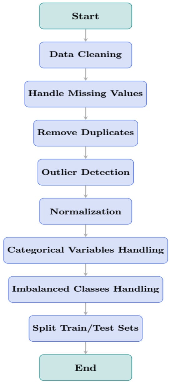
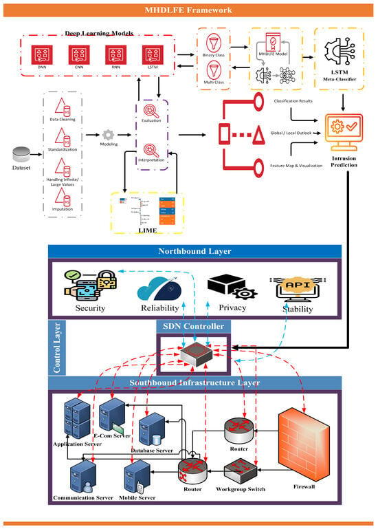
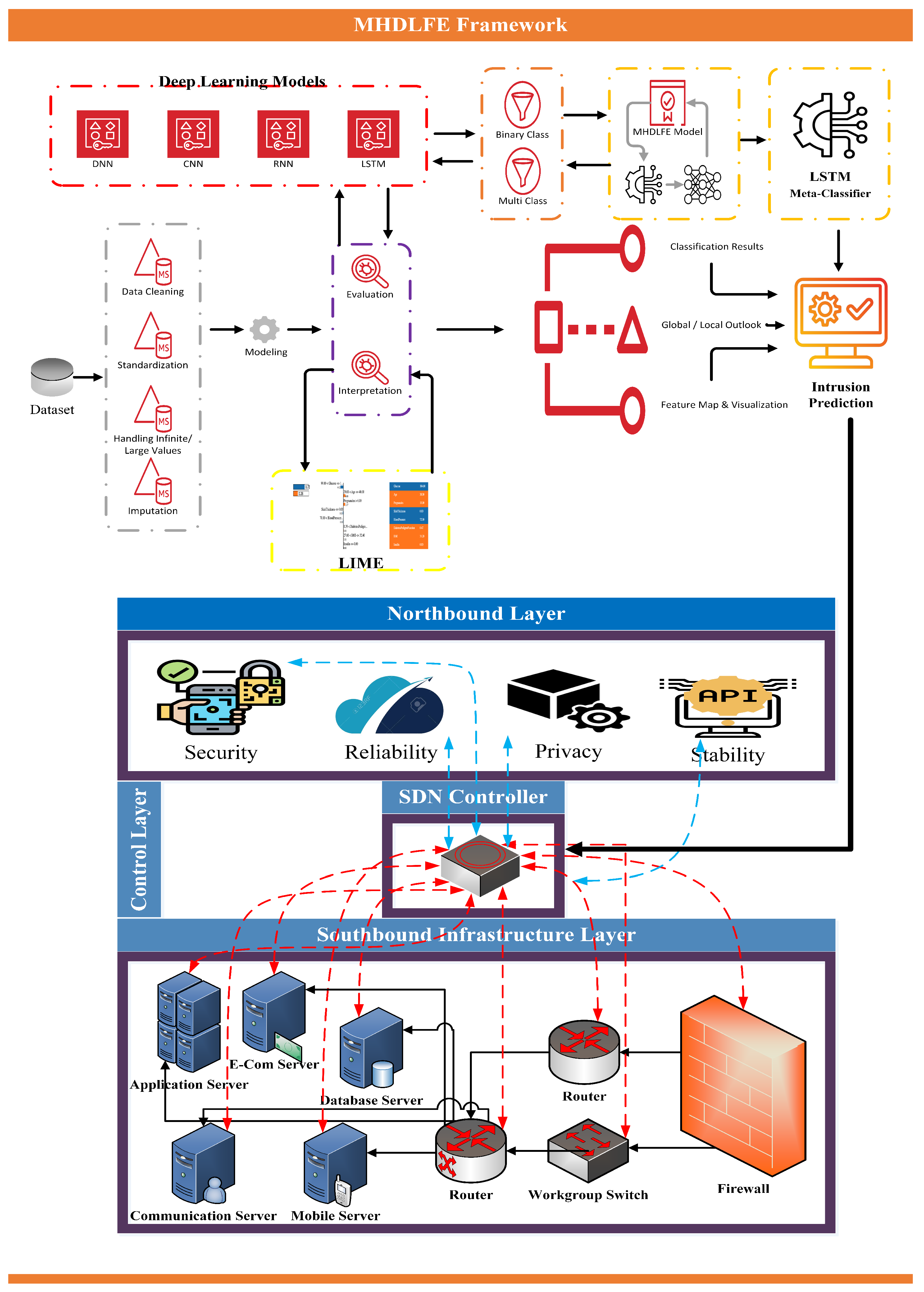
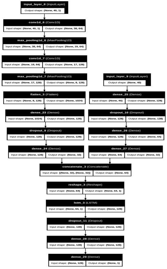
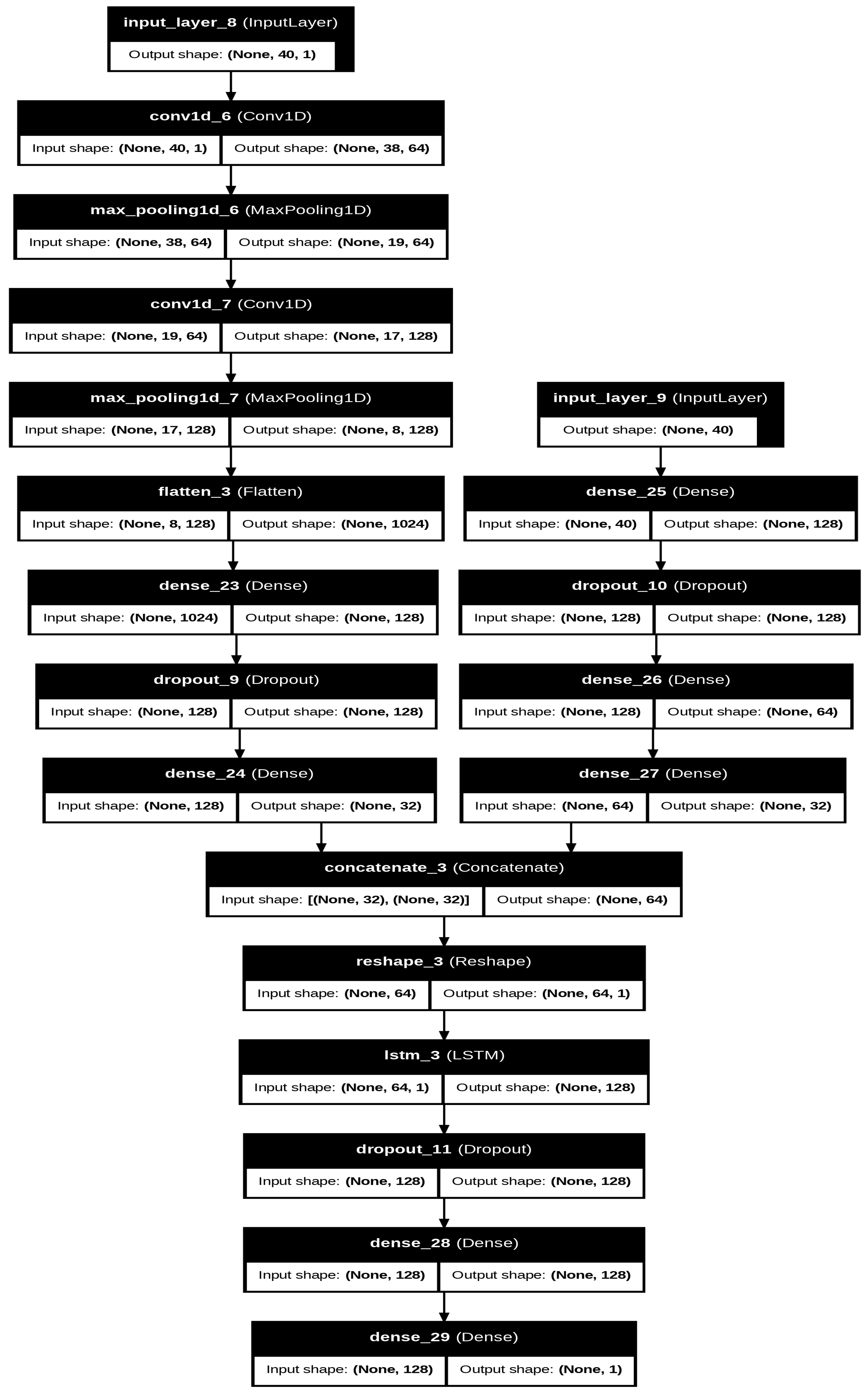
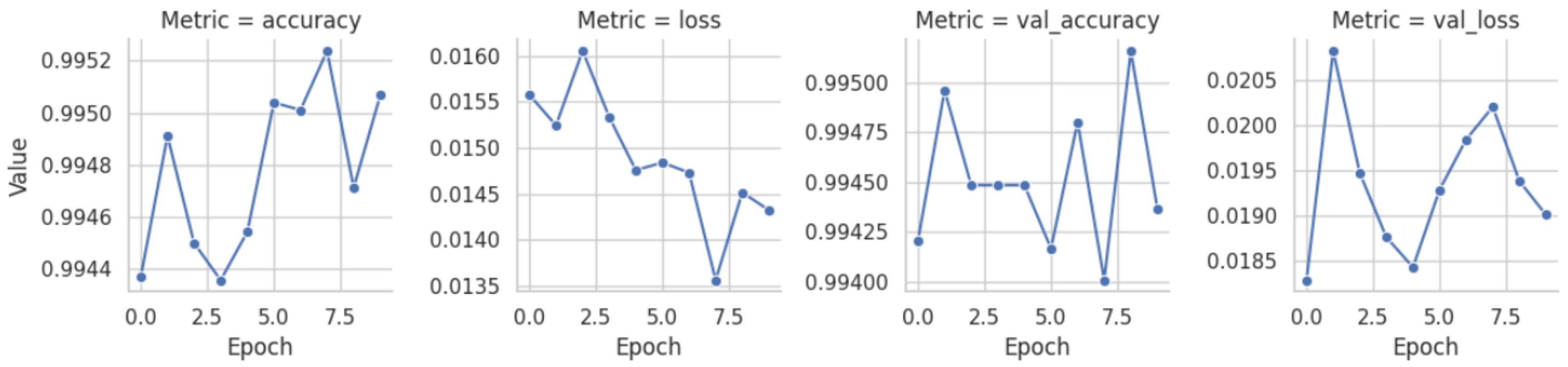
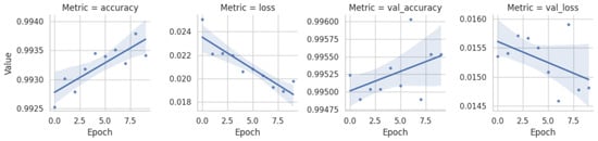
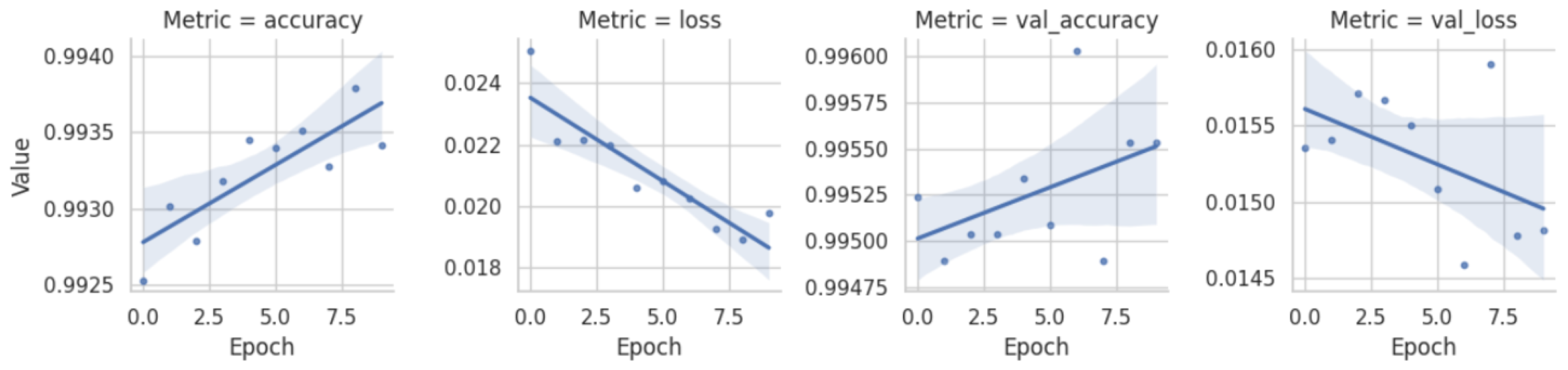
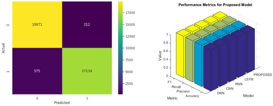
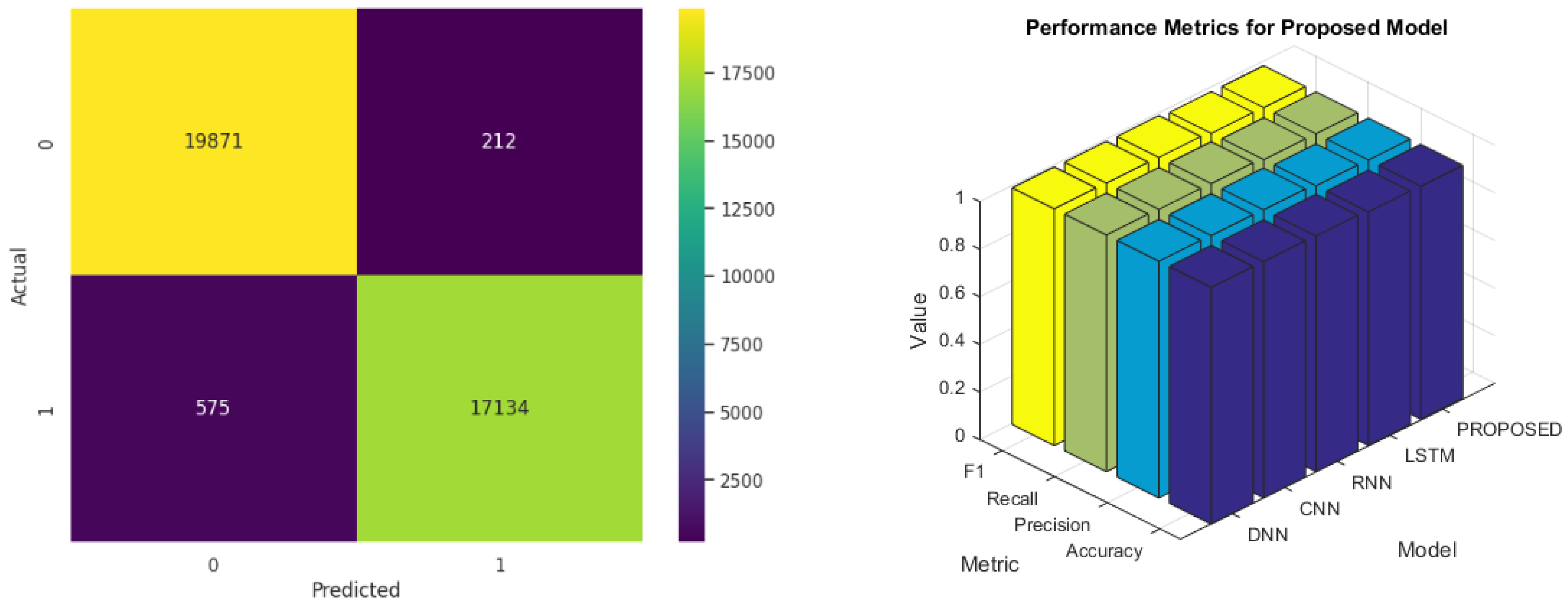
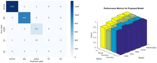
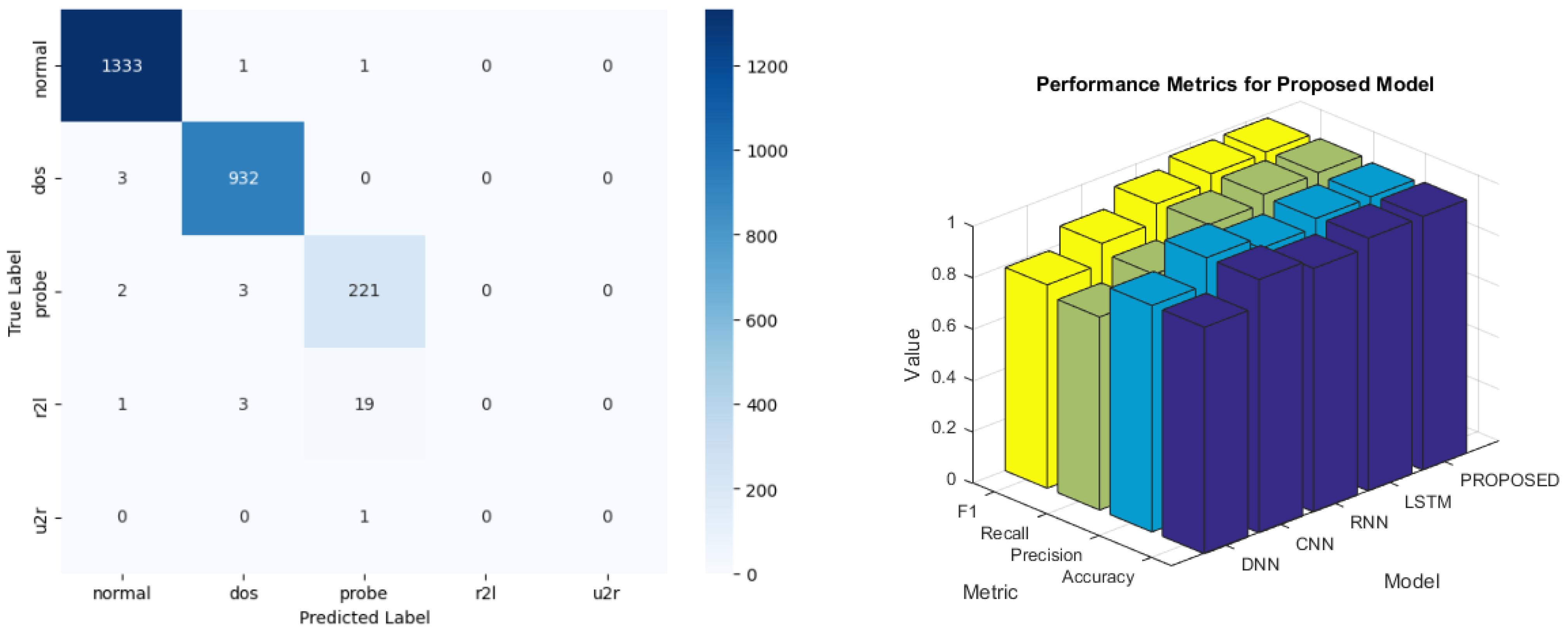
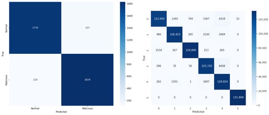
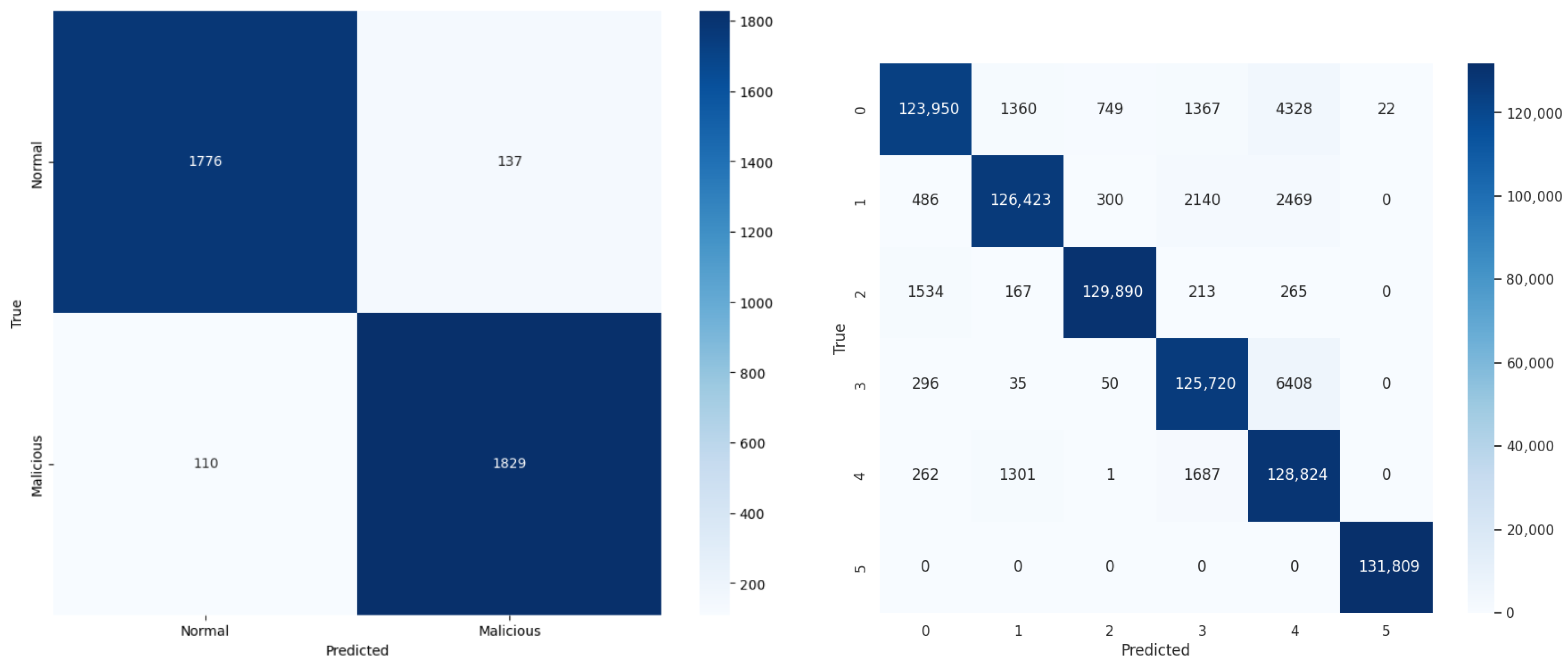
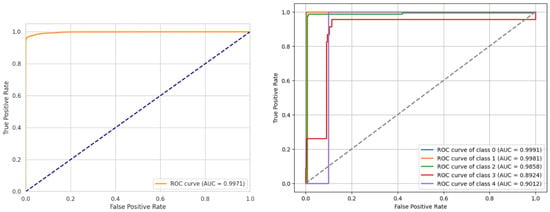
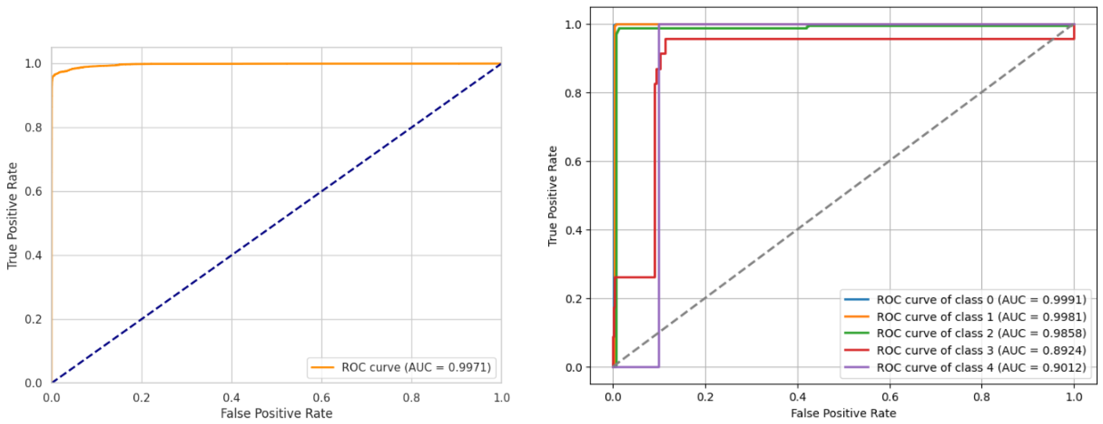
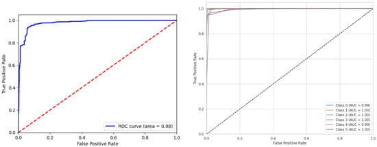
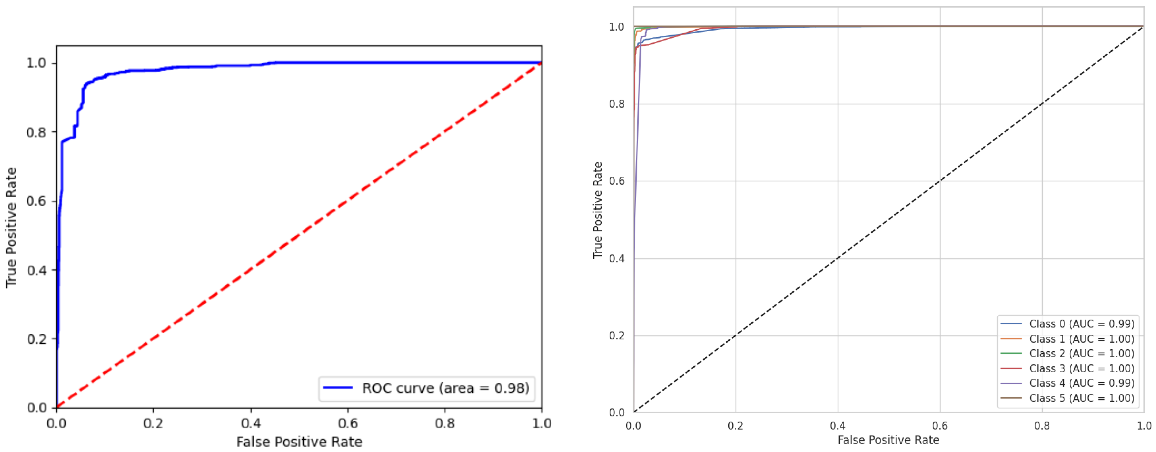
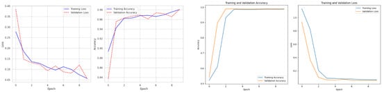
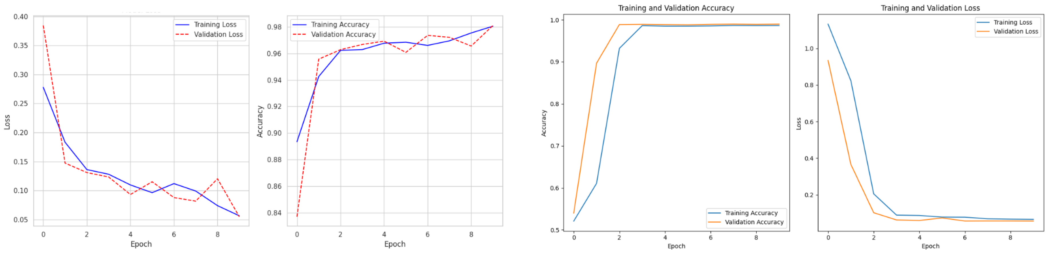


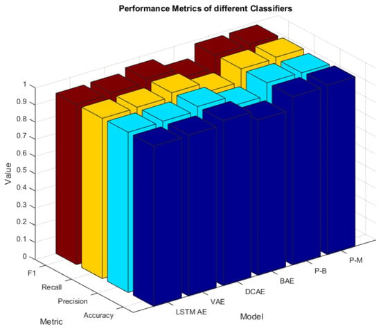
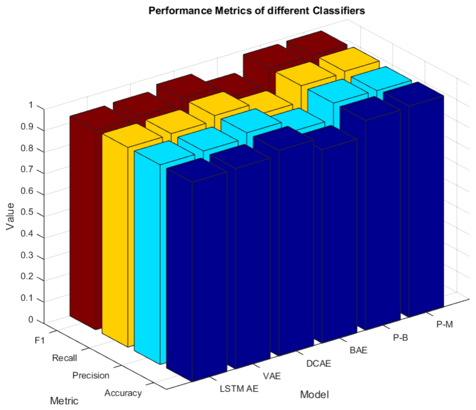
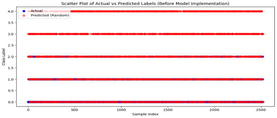
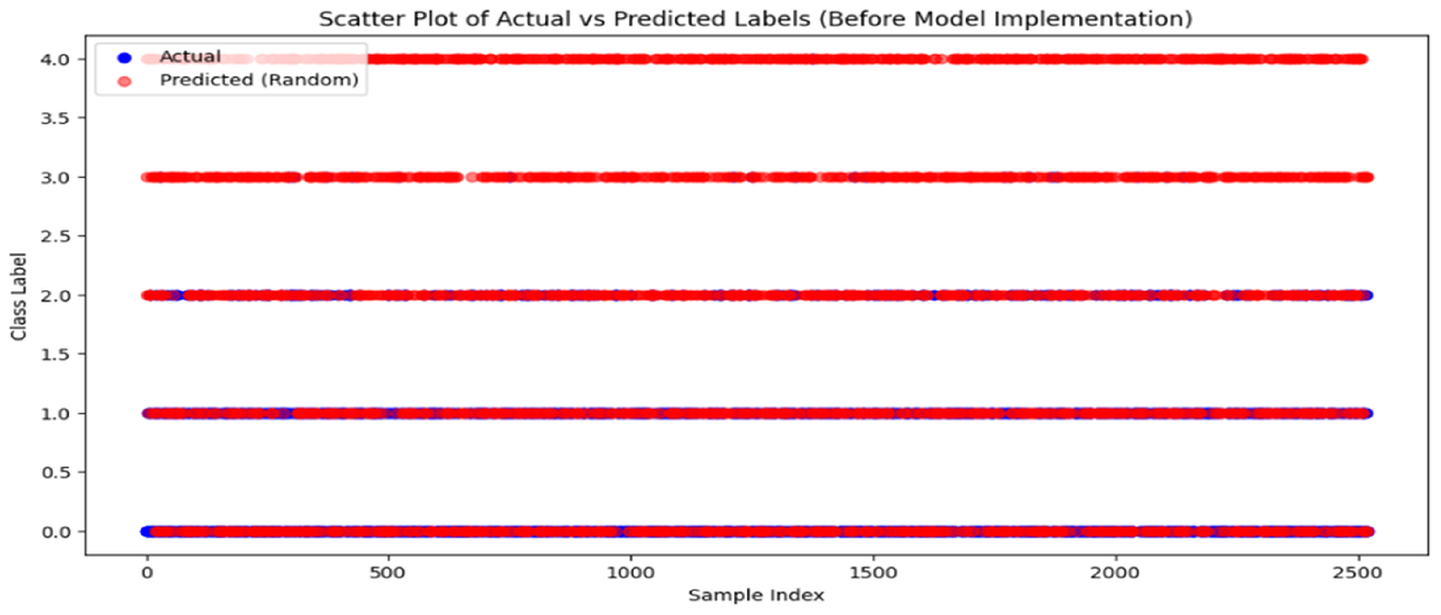
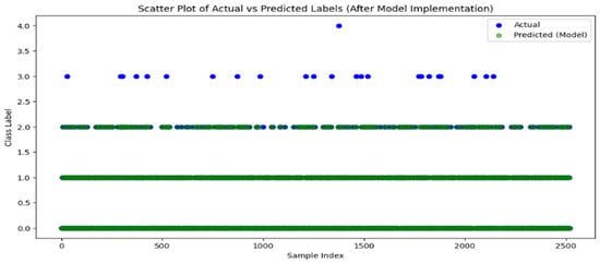
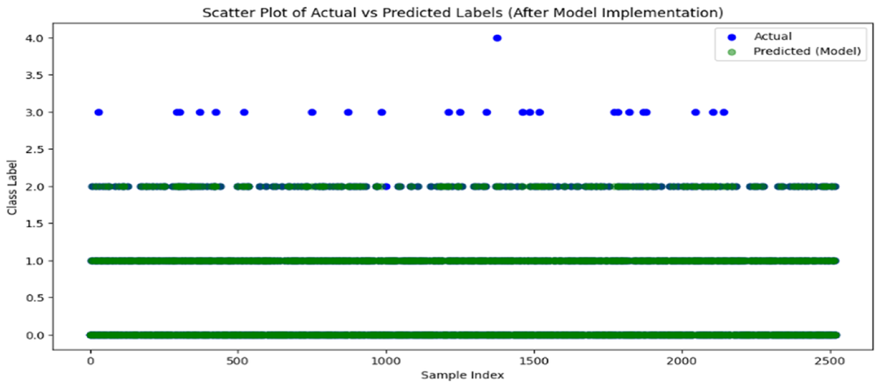
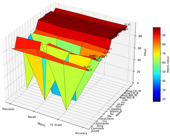
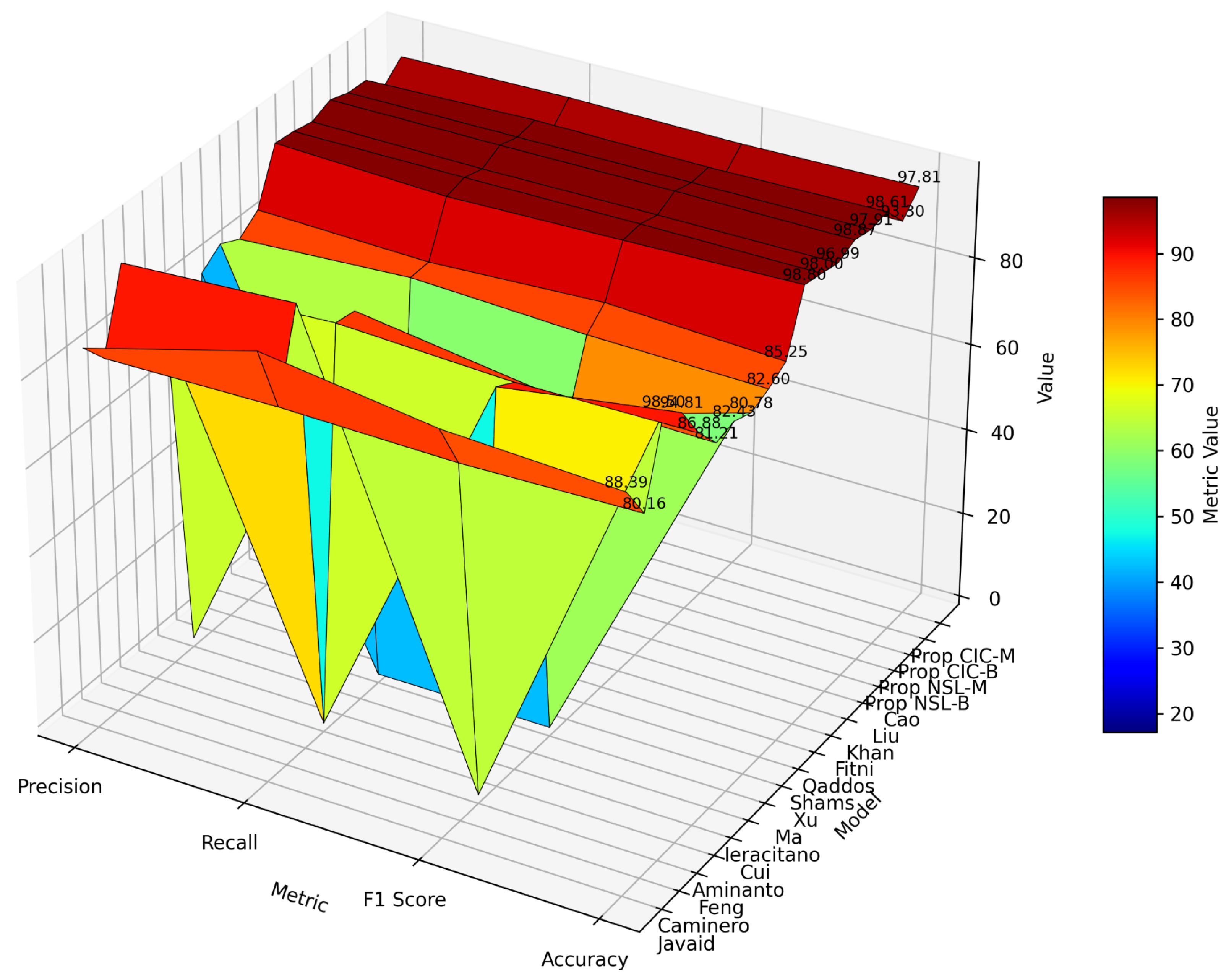
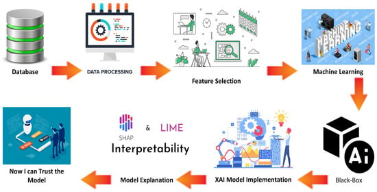
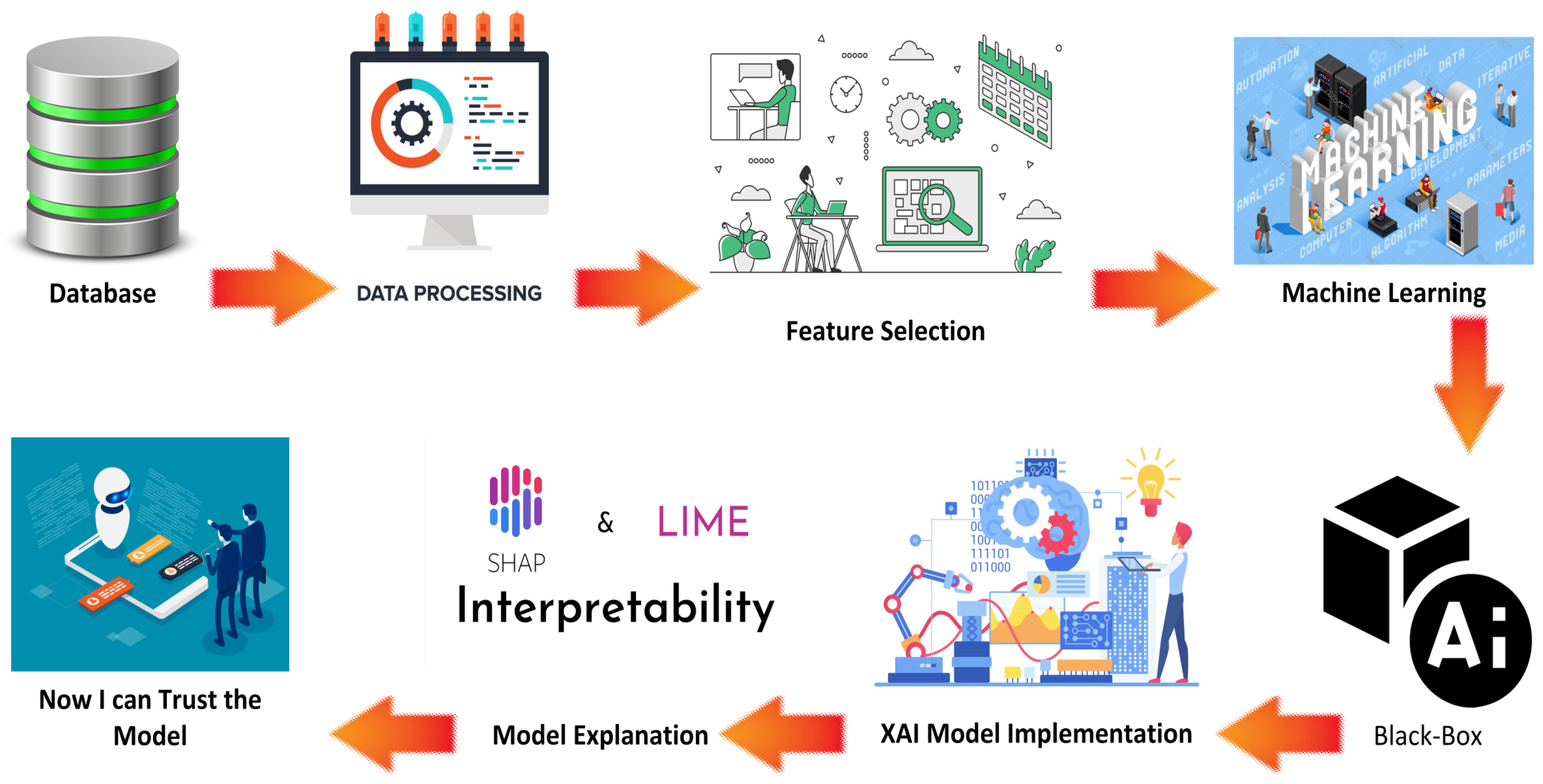
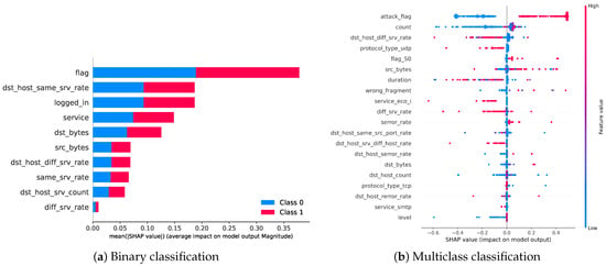
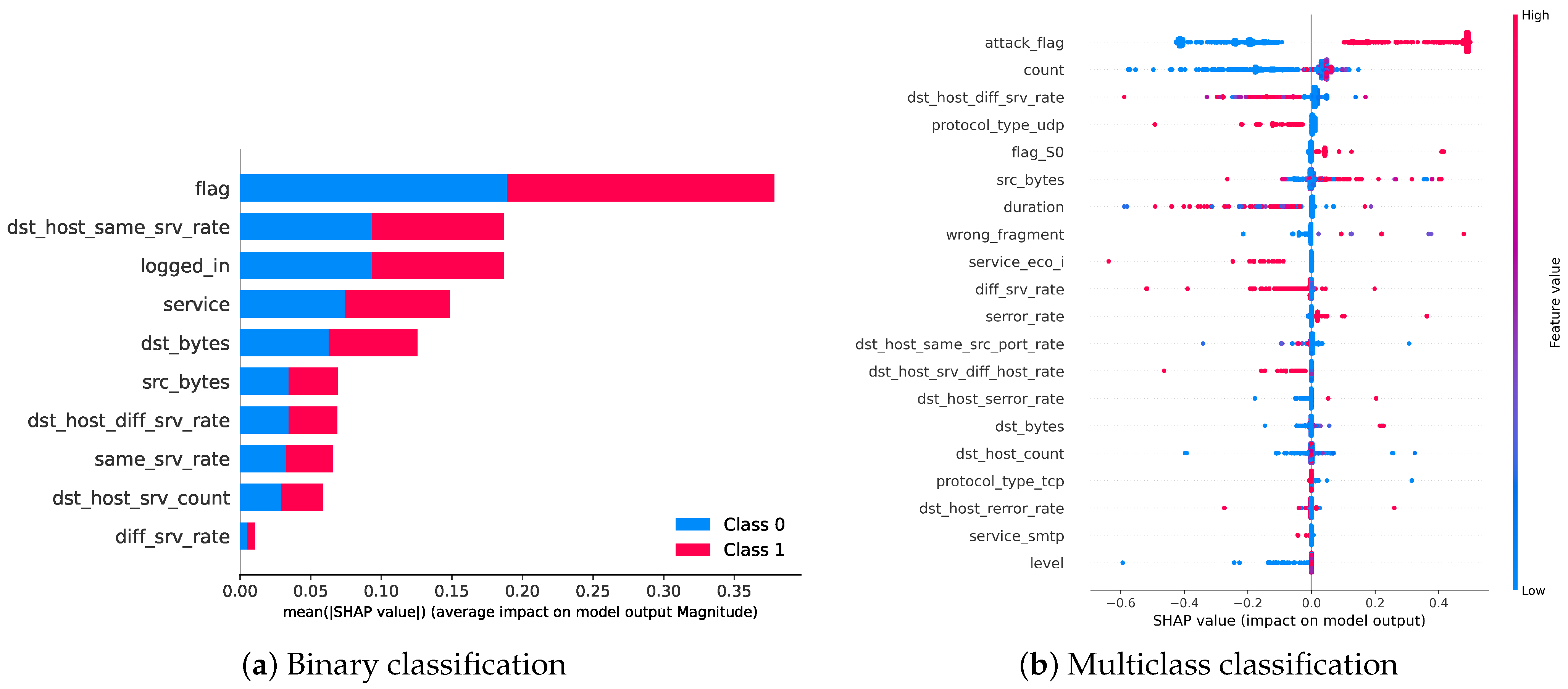
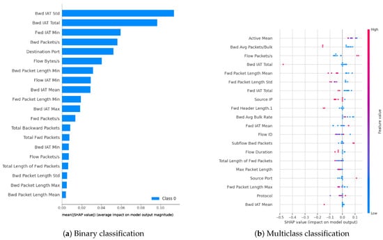
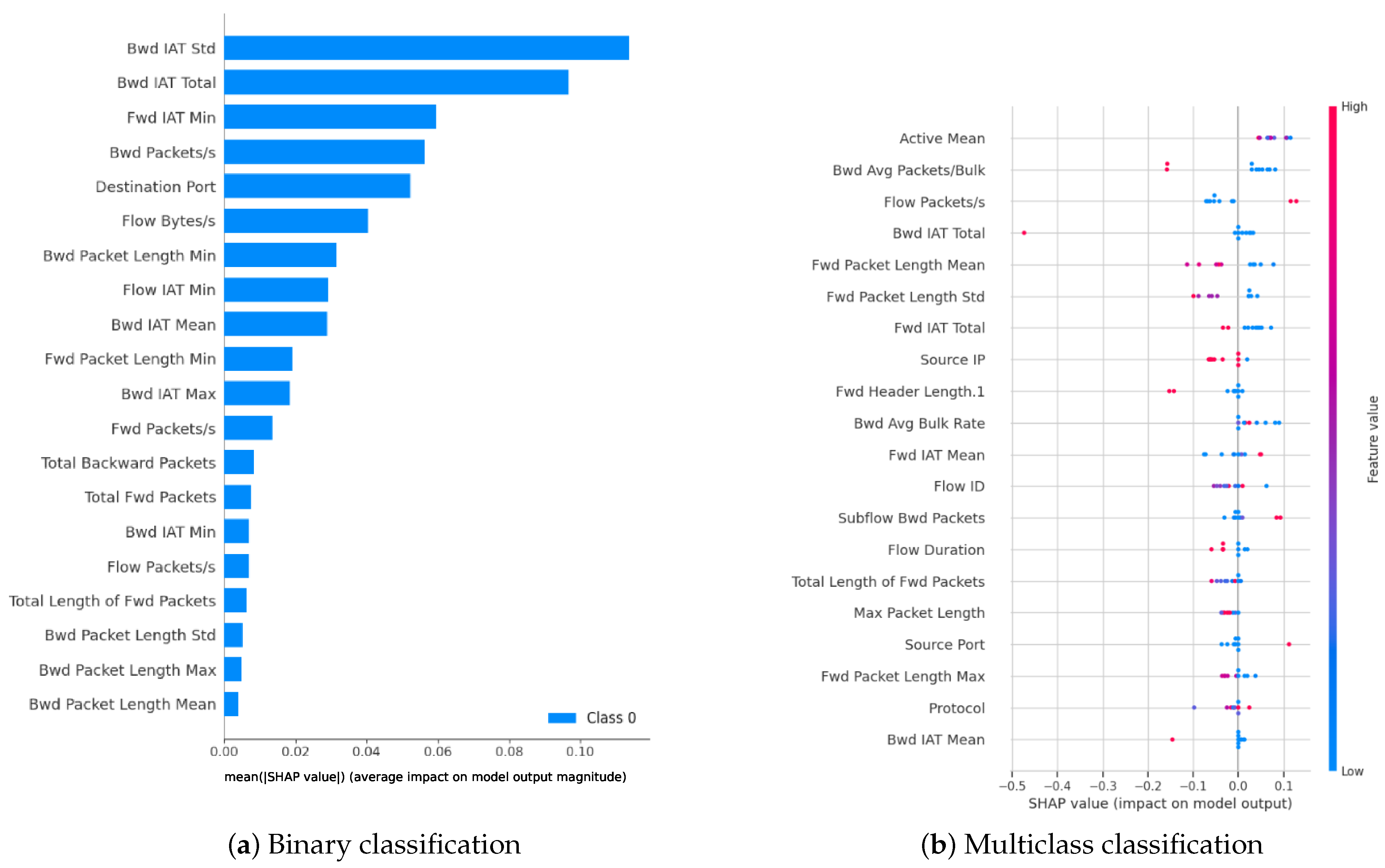
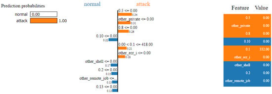
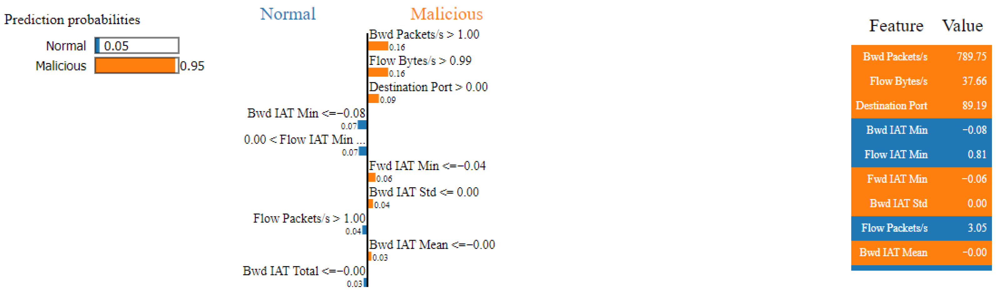
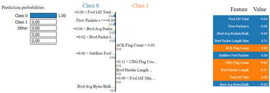
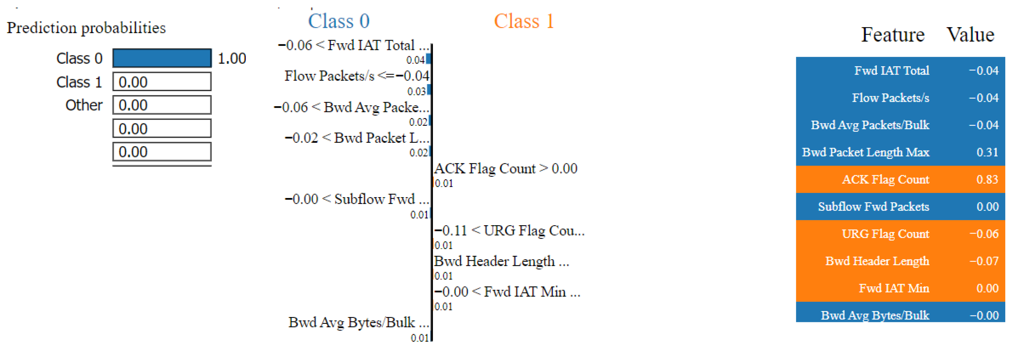
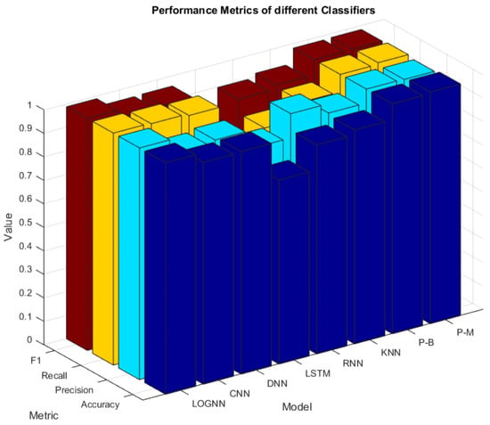
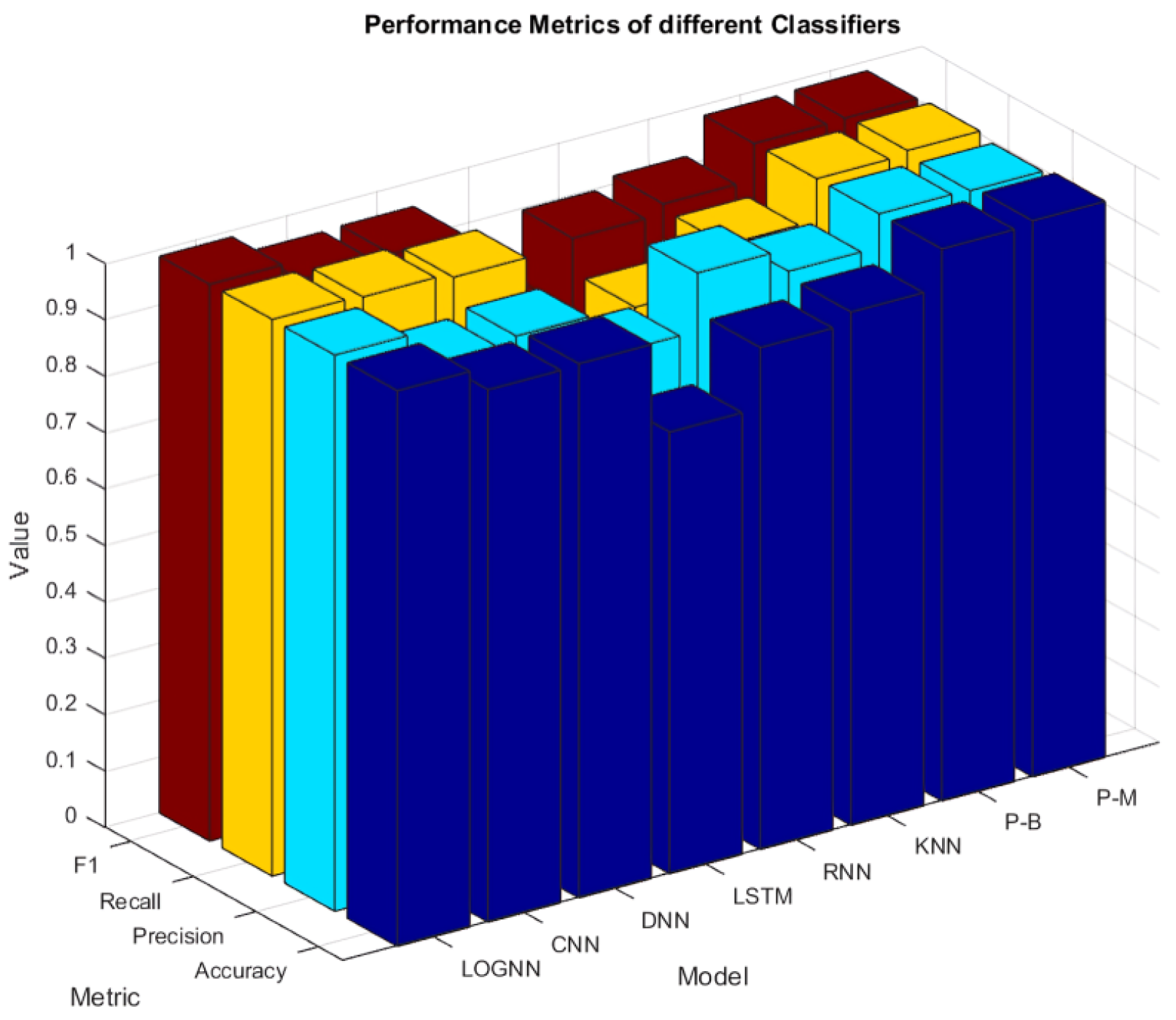

Disclaimer/Publisher’s Note: The statements, opinions and data contained in all publications are solely those of the individual author(s) and contributor(s) and not of MDPI and/or the editor(s). MDPI and/or the editor(s) disclaim responsibility for any injury to people or property resulting from any ideas, methods, instructions or products referred to in the content. |
© 2026 by the authors. Licensee MDPI, Basel, Switzerland. This article is an open access article distributed under the terms and conditions of the Creative Commons Attribution (CC BY) license.