Interval Estimation for the Difference and Ratio of Variances Under the Zero-Inflated Two-Parameter Rayleigh Distribution

Abstract

The zero-inflated two-parameter Rayleigh (ZITR) distribution provides a flexible framework for modeling data with excess zeros and positive observations following a two-parameter Rayleigh distribution. It is particularly suitable for right-skewed data and has applications in areas such as road traffic mortality and survival analysis. This study develops and compares several methods for constructing confidence intervals for the difference and ratio of variances from two independent ZITR populations. The considered methods include Bayesian approaches based on Markov Chain Monte Carlo (MCMC) and highest posterior density (HPD) intervals, as well as the generalized confidence interval (GCI), method of variance estimates recovery (MOVER), approximate normal (AN), percentile bootstrap (PB), and bootstrap with standard error (BS). The performance of these methods is evaluated via Monte Carlo simulations under various parameter settings and sample sizes, using coverage probability and expected interval length as performance criteria. The results indicate that the Bayesian HPD method generally performs well across a wide range of scenarios. A real-data application using road traffic mortality data from January 2025 in Chanthaburi and Narathiwat provinces is also presented, demonstrating the practical usefulness of the proposed approaches for comparing the variance structure between the two regions.

1. Introduction

Probability distributions form a fundamental basis of statistical analysis, as they describe the behavior of data or random variables and summarize key characteristics such as dispersion, skewness, and kurtosis through a set of unknown parameters [1]. The choice of an appropriate distribution depends largely on the nature of the data under study. For continuous right-skewed data, commonly used distributions include the Rayleigh, Weibull, exponential, Gamma, and lognormal distributions [2,3].

The coexistence of excess zeros and occasional extreme values poses challenges for statistical analysis, particularly when high estimation accuracy is required. Applying standard continuous distributions without accounting for the large proportion of zeros may lead to biased inference and inflated variability. A fundamental framework for handling such data was introduced by Aitchison [4], who proposed a mixed-distribution model in which observations arise from two components: a degenerate distribution assigning positive probability to zero and a continuous distribution governing positive outcomes. This idea provided the foundation for later developments in delta and zero-inflated models. Subsequently, Fletcher [5] and Lecomte et al. [6] extended skewed continuous distributions by incorporating an explicit probability mass at zero, enhancing model flexibility for datasets with many zeros. Lambert [7] later formalized the zero-inflated modeling framework, particularly for cases where the observed number of zeros exceeds that expected under standard count models. This concept was further extended to continuous settings, allowing zero and positive observations to arise from distinct underlying processes. As a result, zero-inflated models have been widely applied in various fields, including environmental science, biomedicine, actuarial science, and reliability analysis (see [8,9]).

The Rayleigh distribution was originally introduced as a one-parameter model characterized by a scale parameter and is primarily used to describe positively skewed continuous data [10]. In its basic form, the distribution is limited in flexibility, as it accounts mainly for skewness without accommodating location shifts. To address this limitation, the two-parameter Rayleigh distribution was developed by incorporating a location parameter, thereby enhancing its flexibility in modeling a wider range of data patterns. This extended form was discussed in early works such as those of Johnson et al. [11], where the fundamental properties of continuous distributions, including the Rayleigh family, were systematically presented. Subsequently, the two-parameter Rayleigh distribution has been widely studied in statistical inference, particularly for estimating unknown parameters and deriving related measures [12,13]. In addition, recent studies have explored Bayesian estimation approaches for the Rayleigh distribution under different loss functions. For example, Seal et al. [14] investigated Bayesian estimation in the Rayleigh distribution under a distance-type loss function, demonstrating its applicability in modeling lifetime data and improving estimation performance under asymmetric loss structures. This highlights the continued relevance of the Rayleigh distribution in lifetime data analysis and modern inferential frameworks.

In many applied settings, particularly in fields involving real-world data analysis, observations often exhibit a combination of features, including a substantial proportion of zero outcomes together with a positively skewed distribution for positive values. Although the two-parameter Rayleigh distribution has been widely used for modeling right-skewed continuous data, its standard form cannot accommodate structural zeros, which are typically generated by underlying system mechanisms rather than random variation. Ignoring this feature may therefore lead to biased parameter estimates and unreliable statistical inference. To address this limitation, a zero-inflated extension of the two-parameter Rayleigh distribution has been proposed in recent studies [15], in which a point mass at zero is incorporated alongside the continuous Rayleigh component, allowing the data-generating process to be decomposed into a zero-generating mechanism and a positive outcome mechanism. In this study, inference on the difference between parameters and the ratio of population means is also considered within this framework. As a result, the model provides a more flexible framework that better reflects the underlying structure of data characterized by both excess zeros and right-skewed positive observations, making it particularly suitable for such applications.

Variance analysis measures dispersion by describing how observations vary around the mean [1]. It provides insight into the level of risk or uncertainty in a dataset. High variability may indicate instability or reduced predictability; therefore, accurate estimation and comparison of variances are essential for reliable statistical inference and evidence-based decision making.

When comparing the variances of two populations, inference is commonly based on either the difference or the ratio of variances. The difference quantifies the absolute disparity in dispersion, whereas the ratio provides a relative, scale-free comparison. Interval estimation within these frameworks has been widely studied. Bebu and Mathew [16] examined comparisons of means and variances under the bivariate log-normal distribution. Herbert et al. [17] developed confidence intervals for the difference between two independent variances using an analytical approach. Wongyai and Suwan [18] proposed confidence interval methods for the ratio of non-normal variances based on a kurtosis-based estimator. Subsequently, Maneerat et al. [19] and Khooriphan et al. [20] developed interval procedures for variance differences under skewed distributions with excess zeros. Similarly, Ratasukharom et al. [21] constructed confidence intervals for both the difference and the ratio of variances under the zero-modified Birnbaum–Saunders distribution. Puggard et al. [22] further developed confidence intervals for comparing variances of two independent Birnbaum–Saunders distributions. Despite these contributions, no study has addressed interval estimation for the difference and ratio of variances under the zero-inflated two-parameter Rayleigh distribution, leaving a gap in the literature on variance comparison for non-normal continuous models.

This study develops confidence intervals for both the difference and the ratio of variances between two zero-inflated two-parameter Rayleigh populations. These measures provide complementary perspectives: the variance difference reflects absolute disparity, whereas the variance ratio offers a relative comparison. Seven inferential approaches are considered: Bayesian Markov Chain Monte Carlo (MCMC), Bayesian highest posterior density (HPD) intervals, the asymptotic approximate normal (AN), the generalized confidence interval (GCI), the method of variance estimates recovery (MOVER), the percentile bootstrap (PB), and the bootstrap standard error method (BS). Their performance is evaluated through simulation using coverage probability and expected interval length.

In this study, an empirical application is presented using accident-related mortality data from January 2025 in Narathiwat and Chanthaburi provinces, Thailand. The data exhibit pronounced right-skewness and contain a large number of zero observations, corresponding to districts with no reported fatalities. Differences in demographic structure, infrastructure, and transportation conditions between the two provinces provide a meaningful basis for examining both absolute and relative measures of dispersion. By integrating methodological development, simulation-based evaluation, and real-data analysis, this study offers practical guidance for comparative inference on dispersion parameters in zero-inflated continuous models, with particular emphasis on the two-parameter Rayleigh distribution.

2. Materials and Methods

Let $X_{ij}=(X_{i1},\dots ,X_{i{n}_i})$ for $i=1,2,j=1,2,\dots ,n_i,$ be independent random samples drawn from a zero-inflated two-parameter Rayleigh model with parameters ${\delta }_i$, ${\lambda }_i$, and ${\mu }_i$ denoted by $X_{ij}({\mu }_i,{\lambda }_i,{\delta }_i)$. Here, ${\delta }_i$ ($0\le {\delta }_i\le 1$) denotes the probability mass at zero, whereas ${\lambda }_i$ and ${\mu }_i$ correspond to the scale and location parameters of the underlying Rayleigh component. The probability density function (PDF) [13] is given by

$$f\left(x_{ij};{\mu }_i,{\lambda }_i,{\delta }_i\right)=\left\{\begin{array}{c}{\delta }_i;x_{ij}=0\\ \left(1-{\delta }_i\right)2{\lambda }_i({\mathrm{x}}_{ij}-{\mu }_i){\mathrm{e}}^{-{\lambda }_i{\left(x_{ij}-{\mu }_i\right)}^2};x_{ij}>{\mu }_i,\end{array}\right.$$

(1)

where $P(X_{ij}=0)={\delta }_i.$ The sample contains $n_i$ observations, which can be partitioned into $n_{i\left(0\right)}$ zero observations and $n_{i\left(1\right)}$ positive observations, with $n_i=n_{i\left(0\right)}+n_{i\left(1\right)}.$ The number of zero observations follows a binomial distribution, $n_{i\left(0\right)}\sim \mathrm{Bin}(n_i,{\delta }_i).$ Accordingly, the maximum likelihood estimator of the zero-inflation parameter is ${\widehat{\delta }}_i={\displaystyle \frac{n_{i\left(0\right)}}{n_i}}.$ The unknown parameters ${\mu }_i$ and ${\lambda }_i$ are estimated using maximum likelihood estimation. Since closed-form solutions are not available [13,23], numerical methods are employed. The estimator of the location parameter ${\mu }_i$ is obtained by solving

$${\displaystyle \frac{2{n^2}_{i\left(1\right)}(\overline{x}-\mu )}{{\displaystyle \sum _{j=1}^{n_{i\left(1\right)}}}{(x_{ij}-{\mu }_i)}^2}}=\sum _{j=1}^{n_{i\left(1\right)}}{(x_{ij}-{\mu }_i)}^{-1},$$

which is solved numerically. Once ${\widehat{\mu }}_i$ is obtained, the maximum likelihood estimator of the scale parameter is

$${\widehat{\lambda }}_i={\displaystyle \frac{n_{i\left(1\right)}}{{\displaystyle \sum _{j=1}^{n_{i\left(1\right)}}}{(x_{ij}-{\mu }_i)}^2}}.$$

In practice, the profile log-likelihood is maximized, and the root-finding procedure for ${\mu }_i$ is implemented using the uniroot function in R version 4.4.1 with a convergence tolerance of ${10}^{-5}$.

The variance of the zero-inflated two-parameter Rayleigh distribution can be expressed as shown in the following equation, with the full derivation provided in Appendix A:

$$\mathrm{Var}\left(X_i\right)={\xi }_i={\displaystyle \frac{4(1-{\delta }_i)-{(1-{\delta }_i)}^2\pi }{4{\lambda }_i}}+{\displaystyle \frac{{\mu }_i}{\sqrt{{\lambda }_i}}}\sqrt{\pi }{\delta }_i(1-{\delta }_i)+{\mu }_i^2{\delta }_i(1-{\delta }_i).$$

Let $x_1$ and $x_2$ be two independent samples of sizes $n_1$ and $n_2$ drawn from populations with parameters $({\mu }_1,{\lambda }_1,{\delta }_1)$ and $({\mu }_2,{\lambda }_2,{\delta }_2)$, respectively. The parameters of interest are the difference and ratio of the variances, defined as

$$\begin{array}{cc}\hfill & \theta ={\xi }_1-{\xi }_2\hfill \\ \hfill & =\left({\displaystyle \frac{4(1-{\delta }_1)-{(1-{\delta }_1)}^2\pi }{4{\lambda }_1}}+{\displaystyle \frac{{\mu }_1}{\sqrt{{\lambda }_1}}}\sqrt{\pi }{\delta }_1(1-{\delta }_1)+{\mu }_1^2{\delta }_1(1-{\delta }_1)\right)\hfill \\ \hfill & -\left({\displaystyle \frac{4(1-{\delta }_2)-{(1-{\delta }_2)}^2\pi }{4{\lambda }_2}}+{\displaystyle \frac{{\mu }_2}{\sqrt{{\lambda }_2}}}\sqrt{\pi }{\delta }_2(1-{\delta }_2)+{\mu }_2^2{\delta }_2(1-{\delta }_2)\right),\hfill \end{array}$$

(2)

and

$$\tau ={\displaystyle \frac{{\xi }_1}{{\xi }_2}}={\displaystyle \frac{\left(\frac{4(1-{\delta }_1)-{(1-{\delta }_1)}^2\pi }{4{\lambda }_1}+\frac{{\mu }_1}{\sqrt{{\lambda }_1}}\sqrt{\pi }{\delta }_1(1-{\delta }_1)+{\mu }_1^2{\delta }_1(1-{\delta }_1)\right)}{\left(\frac{4(1-{\delta }_2)-{(1-{\delta }_2)}^2\pi }{4{\lambda }_2}+\frac{{\mu }_2}{\sqrt{{\lambda }_2}}\sqrt{\pi }{\delta }_2(1-{\delta }_2)+{\mu }_2^2{\delta }_2(1-{\delta }_2)\right)}}.$$

(3)

These statistics are used to construct confidence intervals for the variance difference $\theta$ and the variance ratio $\tau$ using seven proposed methods.

2.1. Bayesian Credible Interval

The Bayesian credible interval integrates prior information with observed data to update uncertainty about model parameters through the posterior distribution [24]. In this study, it is used to assess both the difference and the ratio of two population variances. Since the posterior distributions are not available in closed form, inference relies on Markov Chain Monte Carlo (MCMC) sampling [25], and interval estimates are obtained using highest posterior density (HPD) intervals [26], which allow direct probabilistic interpretation.

2.1.1. Bayesian Markov Chain Monte Carlo (MCMC)

Two independent samples, $X_{ij}=(X_{i1},\dots ,X_{i{n}_i})$ for $i=1,2$ and $j=1,2,\dots ,n_i$, are assumed to follow a zero-inflated two-parameter Rayleigh distribution. The focus of this study is Bayesian inference for two measures of variability: the variance difference $\theta$ and the variance ratio $\tau$, both defined in terms of the model parameters. Since the posterior distribution does not have a closed-form expression, simulation-based inference is required. A Markov Chain Monte Carlo (MCMC) algorithm is applied to obtain posterior samples, from which the quantities $\theta$ and $\tau$ are evaluated iteratively to construct their empirical posterior distributions.

The model parameters are assigned the following prior distributions: a gamma prior for the scale parameter $\lambda$, a uniform prior for the location parameter $\mu$, and a beta prior for the zero-inflation parameter $\delta$. These prior choices are used to ensure parameter constraints and improve numerical stability. All computations are implemented in R using the R2OpenBUGS version 3.2.1 package. Bayesian credible intervals for difference variances $\theta$ and ratio variances $\tau$ are obtained from the corresponding posterior quantiles based on the MCMC output.

Accordingly, the posterior samples obtained from the MCMC procedure are used to construct the Bayesian credible intervals for $\theta$ and $\tau$, defined as follows:

$$C{I}_{\theta \left(\mathrm{MCMC}\right)}=\left(L_{\theta \left(\mathrm{MCMC}\right)},U_{\theta \left(\mathrm{MCMC}\right)}\right)=\left({\theta }_{\mathrm{MCMC}}\left(\alpha /2\right),{\theta }_{\mathrm{MCMC}}\left(1-\alpha /2\right)\right),$$

(4)

and

$$C{I}_{\tau \left(\mathrm{MCMC}\right)}=\left(L_{\tau \left(\mathrm{MCMC}\right)},U_{\tau \left(\mathrm{MCMC}\right)}\right)=\left({\tau }_{\mathrm{MCMC}}\left(\alpha /2\right),{\tau }_{\mathrm{MCMC}}\left(1-\alpha /2\right)\right).$$

(5)

The construction of credible intervals for the variances difference and variances ratio using Bayesian MCMC is summarized in Algorithm 1.

Algorithm 1 Bayesian Markov Chain Monte Carlo (MCMC)

1. Random samples are generated from the zero-inflated two-parameter Rayleigh distribution $X_{ij}\sim \mathrm{ZITR}({\mu }_i,{\lambda }_i,{\delta }_i),i=1,2,$ and prior distributions are assigned to the unknown parameters. In particular, the zero-inflation parameter follows a Beta distribution, the scale parameter follows a Gamma distribution, and the location parameter is modeled using a Uniform distribution, expressed as $${\delta }_i\sim \mathrm{Beta}({\alpha }_{1i},{\beta }_{1i}),{\lambda }_i\sim \mathrm{Gamma}({\alpha }_{2i},{\beta }_{2i}),{\mu }_i\sim \mathrm{Uniform}(a_{1i},b_{1i}),$$ where the hyperparameters are determined via a trial-and-error calibration to ensure appropriate prior specification. 2. A Bayesian estimation framework is implemented via a Gibbs sampling algorithm. The procedure is carried out in R with OpenBUGS version 3.2.3 to generate samples from the joint posterior distribution of the parameters. This approach is used because the posterior distributions are not available in closed form. 3. At each iteration of the Markov Chain Monte Carlo, the quantities of interest are computed, namely the difference of variances $\theta$ and the ratio of variances $\tau$. The MCMC algorithm is run for T iterations, and the first C iterations are discarded as burn-in to mitigate the influence of initial values and to enhance convergence to the stationary distribution. 4. Based on the retained MCMC samples, denoted by ${\widehat{\theta }}_{\mathrm{MCMC}}$ and ${\widehat{\tau }}_{\mathrm{MCMC}}$, the $95\%$ Bayesian credible intervals are constructed using empirical quantiles of the posterior draws, providing interval estimates that reflect posterior uncertainty without relying on asymptotic assumptions.

2.1.2. Bayesian Highest Posterior Density (HPD)

The highest posterior density (HPD) credible interval is defined as a subset of the posterior distribution such that all points within the interval have higher density than those outside, while maintaining the shortest possible interval length [26]. This feature allows the HPD interval to provide a concise summary of parameter uncertainty.

In this study, HPD credible intervals are used to assess the uncertainty of the variance difference and variance ratio, denoted by $\theta$ and $\tau$, respectively. These intervals are derived from posterior samples obtained using the HDInterval package in the R environment. Based on the simulated posterior samples, the two-sided HPD credible interval for $\theta$ and $\tau$ are given by

$$C{I}_{\theta \left(\mathrm{HPD}\right)}=\left(L_{\theta \left(\mathrm{HPD}\right)},U_{\theta \left(\mathrm{HPD}\right)}\right)=\left({\theta }_{\mathrm{HPD}}\left(\alpha /2\right),{\theta }_{\mathrm{HPD}}\left(1-\alpha /2\right)\right),$$

(6)

and

$$C{I}_{\tau \left(\mathrm{HPD}\right)}=\left(L_{\tau \left(\mathrm{HPD}\right)},U_{\tau \left(\mathrm{HPD}\right)}\right)=\left({\tau }_{\mathrm{HPD}}\left(\alpha /2\right),{\tau }_{\mathrm{HPD}}\left(1-\alpha /2\right)\right).$$

(7)

The procedure for constructing Bayesian HPD credible intervals for the variance difference and variance ratio under the zero-inflated two-parameter Rayleigh distribution is summarized in Algorithm 2.

Algorithm 2 Bayesian Highest Posterior Density (HPD)

1. Draw random samples from $X_{ij}\sim \mathrm{ZITR}({\mu }_i,{\lambda }_i,{\delta }_i)$ for $i=1,2$. Specify prior distributions for the model parameters as follows: $${\delta }_i\sim \mathrm{Beta}({\alpha }_{1i},{\beta }_{1i}),{\lambda }_i\sim \mathrm{Gamma}({\alpha }_{2i},{\beta }_{2i}),{\mu }_i\sim \mathrm{Uniform}(a_{1i},b_{1i}),$$ where the hyperparameters are determined based on prior information or preliminary investigation. 2. Apply a Gibbs sampling scheme implemented in R through OpenBUGS to obtain samples from the joint posterior distribution. 3. At each iteration, evaluate the variance difference ${\theta }^{\left(t\right)}$ and the variance ratio ${\tau }^{\left(t\right)}$. The Markov chain is run for T iterations, with the first C samples discarded as burn-in to reduce the effect of initial values. 4. Based on the retained posterior draws of $\theta$ and $\tau$, construct highest posterior density intervals using the HDInterval package in R. The corresponding 95% Bayesian HPD credible intervals for $\theta$ and $\tau$ are then obtained.

2.2. Generalized Confidence Interval (GCI)

The generalized confidence interval (GCI) approach provides an inferential framework based on generalized pivotal quantities (GPQs) and is particularly useful when the sampling distribution of an estimator is not available in closed form [27]. A generalized pivotal quantity is constructed so that its distribution is free of unknown nuisance parameters, while its observed value depends only on the sample data. This feature allows its distribution to be approximated directly through simulation, without relying on asymptotic results.

Wu and Hsieh [28] and Krishnamoorthy et al. [23] further extended this approach. Wu and Hsieh employed variance-stabilizing transformations to obtain tractable forms, whereas Krishnamoorthy and co-authors proposed alternative GPQ constructions to facilitate interval estimation.

Following these developments, the generalized pivotal quantities for the variance difference and variance ratio under the proposed model are defined as

$$Q_{\theta }=Q_{{\xi }_1}-Q_{{\xi }_2},$$

(8)

and

$$Q_{\tau }={\displaystyle \frac{Q_{{\xi }_1}}{Q_{{\xi }_2}}},$$

(9)

respectively, where

$$Q_{{\xi }_i}={\displaystyle \frac{4\left(1-Q_{{\delta }_i}\right)-{\left(1-Q_{{\delta }_i}\right)}^2\pi }{4Q_{{\lambda }_i}}}+{\displaystyle \frac{Q_{{\mu }_i}}{\sqrt{Q_{{\lambda }_i}}}}\sqrt{\pi }{Q}_{{\delta }_i}\left(1-Q_{{\delta }_i}\right)+Q_{{\mu }_i}^2{Q}_{{\delta }_i}\left(1-Q_{{\delta }_i}\right).$$

Since the distributions of $Q_{\theta }$ and $Q_{\tau }$ do not involve unknown parameters, their empirical distributions can be obtained via Monte Carlo simulation. The $(1-\alpha )$ generalized confidence intervals are then constructed from the empirical quantiles of $Q_{\theta }$ and $Q_{\tau }$. Specifically,

$$C{I}_{\theta \left(\mathrm{GCI}\right)}=\left(Q_{\theta }\left(\alpha /2\right),Q_{\theta }\left(1-\alpha /2\right)\right),$$

(10)

and

$$C{I}_{\tau \left(\mathrm{GCI}\right)}=\left(Q_{\tau }\left(\alpha /2\right),Q_{\tau }\left(1-\alpha /2\right)\right).$$

(11)

Here, $Q_{\theta }(\alpha /2)$ and $Q_{\tau }(\alpha /2)$ denote the $100(\alpha /2)$th percentiles of $Q_{\theta }$ and $Q_{\tau }$, respectively. The procedure for constructing these intervals under the zero-inflated two-parameter Rayleigh distribution is summarized in Algorithm 3.

Algorithm 3 Generalized Confidence Interval (GCI)

1. Generate random samples from $X_{ij}\sim \mathrm{ZITR}({\mu }_i,{\lambda }_i,{\delta }_i)$ for $i=1,2$. 2. Obtain MLEs of the parameters, denoted as ${\widehat{a}}_i$ and ${\widehat{b}}_i$. 3. For each group, generate simulated observations from the two-parameter Rayleigh component of the model. These simulated values can be produced, for instance, under the parameter setting $(a=0,b=1)$, or equivalently $(\mu =0,\lambda =0.5)$. 4. For each simulated sample, compute the corresponding maximum likelihood estimates, ${\widehat{a}}_i^{\ast }$ and ${\widehat{b}}_i^{\ast }$, to be used in constructing the generalized pivotal quantities. 5. Construct the generalized pivotal quantities for the zero-inflation and Rayleigh parameters as follows: For the zero-inflation parameter, define $T=2\sqrt{n}\left(arcsin\sqrt{\widehat{\delta }}-arcsin\sqrt{\delta }\right)\sim N(0,1)$ and compute $Q_{\delta }={sin}^2\left(arcsin\sqrt{\widehat{\delta }}-{\displaystyle \frac{T}{2\sqrt{n}}}\right).$ For the Rayleigh parameters, define $Q_a=\widehat{a}-\widehat{b}{\displaystyle \frac{{\widehat{a}}^{\ast }}{{\widehat{b}}^{\ast }}},Q_b={\displaystyle \frac{\widehat{b}}{{\widehat{b}}^{\ast }}},Q_{\mu }=Q_a,Q_{\lambda }={\displaystyle \frac{1}{2Q_b^2}}.$ Using these expressions, derive the generalized pivotal quantities for the variance difference and ratio, $Q_{\theta }$ and $Q_{\tau }$. 6. Repeat the above steps q times to approximate the empirical distributions of the generalized pivotal quantities $Q_{\theta }$ and $Q_{\tau }$. 7. Sort the simulated values of $Q_{\theta }$ and $Q_{\tau }$ in ascending order and extract the appropriate percentiles to construct the 95% generalized confidence intervals, as given in Equations (10) and (11).

2.3. Method of Variance Estimates Recovery (MOVER)

Donner and Zou [29] proposed a method for constructing confidence intervals for both the difference and the ratio of two distribution parameters. This approach is particularly useful when deriving analytical expressions for the variances of the estimators is difficult, and thus offers a practical alternative for interval estimation of both measures.

In this study, the confidence intervals for the variance difference and variance ratio, denoted by $\theta$ and $\tau$, are expressed as

$$C{I}_{\theta \left(\mathrm{MOVER}\right)}=\left(L_{\theta \left(\mathrm{MOVER}\right)},U_{\theta \left(\mathrm{MOVER}\right)}\right),$$

(12)

and

$$C{I}_{\tau \left(\mathrm{MOVER}\right)}=\left(L_{\tau \left(\mathrm{MOVER}\right)},U_{\tau \left(\mathrm{MOVER}\right)}\right).$$

(13)

The lower and upper bounds for $\theta$ are given by

$$L_{\theta \left(\mathrm{MOVER}\right)}=\left({\widehat{\xi }}_1-{\widehat{\xi }}_2\right)-\sqrt{{\left({\widehat{\xi }}_1-l_1\right)}^2-{\left(u_2-{\widehat{\xi }}_2\right)}^2},$$

(14)

and

$$U_{\theta \left(\mathrm{MOVER}\right)}=\left({\widehat{\xi }}_1-{\widehat{\xi }}_2\right)+\sqrt{{\left(u_1-{\widehat{\xi }}_1\right)}^2-{\left({\widehat{\xi }}_2-l_2\right)}^2}.$$

(15)

The corresponding bounds for the variance ratio $\tau$ are given by

$$L_{\tau \left(\mathrm{MOVER}\right)}={\displaystyle \frac{{\widehat{\xi }}_1{\widehat{\xi }}_2-\sqrt{{\left({\widehat{\xi }}_1{\widehat{\xi }}_2\right)}^2-l_1{u}_2\left(2{\widehat{\xi }}_1-l_1\right)\left(2{\widehat{\xi }}_2-u_2\right)}}{u_2\left(2{\widehat{\xi }}_2-u_2\right)}},$$

(16)

and

$$U_{\tau \left(\mathrm{MOVER}\right)}={\displaystyle \frac{{\widehat{\xi }}_1{\widehat{\xi }}_2+\sqrt{{\left({\widehat{\xi }}_1{\widehat{\xi }}_2\right)}^2-u_1{l}_2\left(2{\widehat{\xi }}_1-u_1\right)\left(2{\widehat{\xi }}_2-l_2\right)}}{l_2\left(2{\widehat{\xi }}_2-l_2\right)}}.$$

(17)

Here, $(l_1,u_1)$ and $(l_2,u_2)$ denote the confidence intervals for the individual variance parameters, obtained using the generalized confidence interval (GCI) approach. These limits are incorporated into the MOVER framework to construct the confidence intervals for $\theta$ and $\tau$, as outlined in Algorithm 4.

Algorithm 4 Method of Variance Estimates Recovery (MOVER)

1. Generate two independent random samples, $X_{1j}\sim ZITR({\mu }_1,{\lambda }_1,{\delta }_1)$ and $X_{2j}\sim ZITR({\mu }_2,{\lambda }_2,{\delta }_2)$. 2. Obtain the estimates ${\widehat{\xi }}_1$ and ${\widehat{\xi }}_2$ using the generalized confidence interval (GCI) approach. 3. Construct the confidence intervals for ${\xi }_1$ and ${\xi }_2$ based on the GCI procedure. 4. Derive the confidence intervals for $\theta$ and $\tau$ according to Equations (12) and (13).

2.4. Approximate Normal

The normal approximation approach is based on the delta method, which provides an asymptotic variance approximation using a first-order Taylor expansion of the transformation of the estimators [30]. Let $\widehat{\theta }$ and $\widehat{\tau }$ denote the estimators of the difference and ratio of variances, respectively. Their asymptotic variances are obtained using the delta method, and the detailed derivations are omitted here for brevity and provided in Appendix B.

Under the assumption of asymptotic normality, approximate $(1-\alpha )100\%$ confidence intervals are constructed as

$$C{I}_{\theta \left(AN\right)}=\left(\widehat{\theta }-z_{\alpha /2}\sqrt{\widehat{V}(\widehat{\theta })},\widehat{\theta }+z_{\alpha /2}\sqrt{\widehat{V}(\widehat{\theta })}\right),$$

(18)

and

$$C{I}_{\tau \left(AN\right)}=\left(\widehat{\tau }-z_{\alpha /2}\sqrt{\widehat{V}(\widehat{\tau })},\widehat{\tau }+z_{\alpha /2}\sqrt{\widehat{V}(\widehat{\tau })}\right),$$

(19)

where $z_{\alpha /2}$ denotes the upper $\alpha /2$ quantile of the standard normal distribution.

The detailed expressions of $\widehat{V}(\widehat{\theta })$ and $\widehat{V}(\widehat{\tau })$ are obtained using the delta method and are presented in Appendix B. Based on these variance approximations, confidence intervals for the difference and ratio of variances of the zero-inflated two-parameter Rayleigh distribution are constructed according to the procedure described in Algorithm 5.

Algorithm 5 Approximate Normal (AN)

1. Generate two independent random samples, $X_{1j}\sim ZITR({\mu }_1,{\lambda }_1,{\delta }_1)$ and $X_{2j}\sim ZITR({\mu }_2,{\lambda }_2,{\delta }_2)$. 2. Obtain MLEs for ${\widehat{\mu }}_i$, ${\widehat{\lambda }}_i$, and ${\widehat{\delta }}_i$. 3. Compute the variance estimators for the difference and ratio of variances using the delta method (see Appendix A). 4. Construct the confidence interval for the difference and ratio variance based on Equations (18) and (19).

2.5. Bootstrap Method

Bootstrap is a resampling-based technique introduced by Efron and Tibshirani [31]. It approximates the sampling distribution of an estimator by repeatedly drawing samples with replacement from the observed data. This approach is particularly useful when analytical expressions for variance are difficult to obtain or when large-sample approximations are unreliable.

In this study, two bootstrap confidence interval methods are considered: the percentile bootstrap and the bootstrap standard error method. The percentile approach constructs intervals directly from the empirical quantiles of the bootstrap distribution, whereas the standard error method combines the bootstrap estimate of variability with a normal approximation.

2.5.1. Percentile Bootstrap (PB)

The percentile bootstrap is a resampling technique employed to approximate the sampling distribution of a statistic and to obtain confidence intervals without imposing strong parametric assumptions. Let $X_{ij}=\left(X_{i1},X_{i2},\dots ,X_{i{n}_i}\right)$ denote a random sample from $ZITR$. A bootstrap sample $X_i^{\ast b}=\left(X_{i1}^{\ast b},X_{i2}^{\ast b},\dots ,X_{i{n}_i}^{\ast b}\right)$ is obtained by sampling with replacement from the original data, and this procedure is repeated B times.

For each bootstrap sample, the statistics of interest are computed. Let $\theta$ denote the difference between two variances and $\tau$ the ratio of two variances. Denote by $\widehat{\theta }$ and $\widehat{\tau }$ the estimators obtained from the original sample. For the bth bootstrap sample, let ${\widehat{\theta }}^{\ast b}$ and ${\widehat{\tau }}^{\ast b}$ be the corresponding bootstrap estimates for $b=1,2,\dots ,B$. The empirical distributions of these bootstrap replicates are used to determine the confidence limits.

The two-sided percentile bootstrap confidence interval for the difference of variances is defined as

$$C{I}_{\theta \left(PB\right)}=\left(L_{\theta \left(PB\right)},U_{\theta \left(PB\right)}\right)=\left({\widehat{\theta }}^{\ast }\left({\displaystyle \frac{\alpha }{2}}\right),{\widehat{\theta }}^{\ast }\left(1-{\displaystyle \frac{\alpha }{2}}\right)\right),$$

(20)

where ${\widehat{\theta }}^{\ast }\left({\displaystyle \frac{\alpha }{2}}\right)$ and ${\widehat{\theta }}^{\ast }\left(1-{\displaystyle \frac{\alpha }{2}}\right)$ are the empirical ${\displaystyle \frac{\alpha }{2}}$ and $1-{\displaystyle \frac{\alpha }{2}}$ quantiles of the ordered bootstrap estimates ${\widehat{\theta }}^{\ast b}$.

Similarly, the two-sided percentile bootstrap confidence interval for the ratio of variances is given by

$$C{I}_{\tau \left(PB\right)}=\left(L_{\tau \left(PB\right)},U_{\tau \left(PB\right)}\right)=\left({\widehat{\tau }}^{\ast }\left({\displaystyle \frac{\alpha }{2}}\right),{\widehat{\tau }}^{\ast }\left(1-{\displaystyle \frac{\alpha }{2}}\right)\right),$$

(21)

where ${\widehat{\tau }}^{\ast }\left({\displaystyle \frac{\alpha }{2}}\right)$ and ${\widehat{\tau }}^{\ast }\left(1-{\displaystyle \frac{\alpha }{2}}\right)$ denote the corresponding empirical quantiles of the bootstrap distribution.

Thus, the percentile bootstrap provides an approximate $100(1-\alpha )\%$ confidence interval for both the difference and the ratio of variances under the zero-inflated two-parameter Rayleigh model. The detailed implementation steps are summarized in Algorithm 6.

Algorithm 6 Percentile Bootstrap (PB)

1. Generate two independent random samples $X_{ij}=\left(X_{i1},X_{i2},\dots ,X_{i{n}_i}\right)$ from the distribution $ZITR({\mu }_i,{\lambda }_i,{\delta }_i)$ for $i=1,2$ and $j=1,2,\dots ,n_i.$ 2. For each sample, draw a bootstrap sample $X_i^{\ast b}=\left(X_{i1}^{\ast b},X_{i2}^{\ast b},\dots ,X_{i{n}_i}^{\ast b}\right)$ by sampling with replacement from the observed data $x_i$. 3. Using the bth bootstrap sample, obtain the maximum likelihood estimates ${\widehat{\mu }}_i^{\ast b}$, ${\widehat{\lambda }}_i^{\ast b}$, and ${\widehat{\delta }}_i^{\ast b}$ for $i=1,2$. 4. Compute the bootstrap estimates of the variance difference ${\widehat{\theta }}^{\ast b}$ and the variance ratio ${\widehat{\tau }}^{\ast b}$ based on the estimated parameters from Step 3. 5. Repeat Steps 2–4 for $b=1,2,\dots ,B$, where B denotes the total number of bootstrap replications. 6. Arrange the bootstrap values $\left\{{\widehat{\theta }}^{\ast 1},\dots ,{\widehat{\theta }}^{\ast B}\right\}$ and $\left\{{\widehat{\tau }}^{\ast 1},\dots ,{\widehat{\tau }}^{\ast B}\right\}$ in ascending order. 7. Determine the lower and upper bounds of the $100(1-\alpha )\%$ percentile bootstrap confidence intervals for $\theta$ and $\tau$ from the empirical quantiles as defined in Equations (20) and (21).

2.5.2. The Bootstrap with Standard Error (BS)

The bootstrap method with standard error estimation constructs confidence intervals by approximating the variability of an estimator through repeated resampling from the observed data. Unlike conventional procedures, this approach avoids the explicit analytical derivation of the variance of the parameter of interest. Instead, the dispersion of the bootstrap replicates is used to estimate the standard error, providing a practical alternative when the sampling distribution is complex or analytically intractable.

Let $\theta$ and $\tau$ denote the difference and the ratio of variances, respectively, under $ZITR$. Suppose that ${\widehat{\theta }}^{\ast b}$ and ${\widehat{\tau }}^{\ast b}$, $b=1,2,\dots ,B$ are the bootstrap estimates obtained from B resamples. The bootstrap means are defined as

$${\overline{\theta }}^{\ast }={\displaystyle \frac{1}{B}}\sum _{b=1}^B{\widehat{\theta }}^{\ast b},{\overline{\tau }}^{\ast }={\displaystyle \frac{1}{B}}\sum _{b=1}^B{\widehat{\tau }}^{\ast b}.$$

The standard errors are estimated by the sample standard deviations of the bootstrap distributions:

$$SE(\widehat{\theta })=\sqrt{{\displaystyle \frac{1}{B-1}}\sum _{b=1}^B{\left({\widehat{\theta }}^{\ast b}-{\overline{\theta }}^{\ast }\right)}^2},$$

$$SE(\widehat{\tau })=\sqrt{{\displaystyle \frac{1}{B-1}}\sum _{b=1}^B{\left({\widehat{\tau }}^{\ast b}-{\overline{\tau }}^{\ast }\right)}^2}.$$

Accordingly, the two-sided $100(1-\alpha )\%$ confidence interval for the difference of variances is given by

$$C{I}_{\theta \left(BS\right)}=\left(L_{\theta \left(BS\right)},U_{\theta \left(BS\right)}\right)=\left({\overline{\theta }}^{\ast }-Z_{\alpha /2}SE\left(\widehat{\theta }\right),{\overline{\theta }}^{\ast }+Z_{\alpha /2}SE\left(\widehat{\theta }\right)\right),$$

(22)

and the confidence interval for the ratio of variances is

$$C{I}_{\tau \left(BS\right)}=\left(L_{\tau \left(BS\right)},U_{\tau \left(BS\right)}\right)=\left({\overline{\tau }}^{\ast }-Z_{\alpha /2}SE\left(\widehat{\tau }\right),{\overline{\tau }}^{\ast }+Z_{\alpha /2}SE\left(\widehat{\tau }\right)\right),$$

(23)

where $Z_{\alpha /2}$ denotes the upper $\alpha /2$ quantile of the standard normal distribution. The computational steps for constructing these bootstrap confidence intervals are summarized in Algorithm 7.

Algorithm 7 The Bootstrap with Standard Error (BS)

1. Generate two independent random samples $X_{ij}=\left(X_{i1},X_{i2},\dots ,X_{i{n}_i}\right)$ from the distribution $ZITR({\mu }_i,{\lambda }_i,{\delta }_i)$ for $i=1,2$ and $j=1,2,\dots ,n_i.$ 2. For each sample, draw a bootstrap resample $X_i^{\ast b}=\left(X_{i1}^{\ast b},X_{i2}^{\ast b},\dots ,X_{i{n}_i}^{\ast b}\right)$ by sampling with replacement from the observed data. 3. Based on the bth bootstrap sample, compute the estimators of the variance difference ${\widehat{\theta }}^{\ast b}$ and the variance ratio ${\widehat{\tau }}^{\ast b}$. 4. Repeat Steps 2 and 3 for $b=1,2,\dots ,B$, where B denotes the number of bootstrap replications. 5. Calculate the bootstrap means ${\overline{\theta }}^{\ast }={\displaystyle \frac{1}{B}}{\sum }_{b=1}^B{\widehat{\theta }}^{\ast b}$ and ${\overline{\tau }}^{\ast }={\displaystyle \frac{1}{B}}{\sum }_{b=1}^B{\widehat{\tau }}^{\ast b}$, and then evaluate the corresponding standard errors using $SE(\widehat{\theta })=\sqrt{{\displaystyle \frac{1}{B-1}}{\sum }_{b=1}^B{\left({\widehat{\theta }}^{\ast b}-{\overline{\theta }}^{\ast }\right)}^2}$, $SE(\widehat{\tau })=\sqrt{{\displaystyle \frac{1}{B-1}}{\sum }_{b=1}^B{\left({\widehat{\tau }}^{\ast b}-{\overline{\tau }}^{\ast }\right)}^2}.$ 6. Construct the two-sided $100(1-\alpha )\%$ confidence intervals for $\theta$ and $\tau$ using the standard error method as presented in Equations (22) and (23).

3. Results

This study examines the construction of confidence intervals for the difference and ratio of variances under the ZITR distribution. The methods considered include Bayesian Markov Chain Monte Carlo (MCMC) credible intervals, Bayesian highest posterior density (HPD) intervals, generalized confidence intervals (GCI), the method of variance estimates recovery (MOVER), the approximate normal (AN) method, percentile bootstrap (PB), and bootstrap with standard error (BS).

The performance of these methods was evaluated through a Monte Carlo simulation study conducted in the R statistical computing environment. For each configuration, 1000 simulation runs were performed. In the resampling-based approaches, 1000 bootstrap samples were generated for both the percentile bootstrap and bootstrap standard error methods. For the GCI approach, 2500 generalized pivotal quantities were generated in each run.

For the Bayesian methods, posterior inference was obtained using a Markov Chain Monte Carlo algorithm implemented via Gibbs sampling. In each run, 20,000 iterations were generated to approximate the joint posterior distributions of the model parameters. To reduce the influence of initial values and ensure convergence, the first 5000 iterations were discarded as burn-in. The remaining samples were used to compute point estimates and to construct Bayesian MCMC and HPD intervals for both the variance difference and variance ratio. Convergence was assessed using trace plots and by examining the stability of posterior summaries.

The interval estimators were evaluated using two criteria: coverage probability (CP) and expected interval length (EL). A method was considered satisfactory if its CP was close to or exceeded the nominal level of $0.95$ while maintaining a relatively short EL. These criteria provided a balanced assessment of reliability and precision. The detailed computational procedure for CP and EL is summarized in Algorithm 8.

Random samples were generated from the ZITR distribution under various combinations of sample sizes and parameter settings. The sample size pairs considered were $(n_1,n_2)=(20,20),(20,50),(20,70),(20,100),(50,50),(50,70),(50,100),(70,70),(70,100),$$(100,100),(200,200).$ Representative parameter configurations were selected to maintain clarity while ensuring practical relevance. The scale parameters were specified as $({\lambda }_1,{\lambda }_2)=(0.2,0.2),(0.2,1),(1,1),$ and the zero-inflation probabilities were defined as $({\delta }_1,{\delta }_2)=(0.1,0.1),(0.1,0.3),(0.3,0.3).$ These settings covered scenarios with low-to-moderate zero inflation, as well as equal and unequal scale parameters, allowing a comprehensive comparison of the interval estimation methods for the variance difference and ratio under the ZITR distribution.

Algorithm 8 CP and EL for difference and ratio variances of $ZITR$

1. Set the simulation design parameters, including the number of Monte Carlo replications M, sample sizes $n_1$ and $n_2$, number of MCMC iterations T, bootstrap resamples B, and generalized pivotal replications C. Let $({\mu }_i,{\lambda }_i,{\delta }_i)$ for $i=1,2$ denote the model parameters. Define ${\xi }_i$ as the variance of the ith population, and consider the parameters of interest: $$\theta ={\xi }_1-{\xi }_2,\tau ={\displaystyle \frac{{\xi }_1}{{\xi }_2}}.$$ 2. For each replication $m=1,2,\dots ,M$, generate two independent random samples from the zero-inflated two-parameter Rayleigh distribution: $X_{ij}\sim ZITR({\mu }_i,{\lambda }_i,{\delta }_i),i=1,2.$ 3. Apply all competing interval estimation procedures to each generated dataset to obtain confidence intervals for $\theta$ and $\tau$, including: Bayesian MCMC, Bayesian HPD, generalized confidence interval (GCI), MOVER, delta method, percentile bootstrap, and bootstrap standard error methods. 4. For each method and replication, obtain an interval $(L_m,U_m)$ and define an indicator variable: $$P_m=\left\{\begin{array}{cc}1,\hfill & \mathrm{if}\mathrm{the}\mathrm{true}\mathrm{parameter}\mathrm{is}\mathrm{contained}\mathrm{in}\mathrm{the}\mathrm{interval},\hfill \\ 0,\hfill & \mathrm{otherwise}.\hfill \end{array}\right.$$ 5. Compute the corresponding interval length for each method as: ${\mathrm{Length}}_m=U_m-L_m.$ 6. After completing all replications, summarize the performance of each method using: $$\mathrm{CP}={\displaystyle \frac{1}{M}}\sum _{m=1}^M{P}_m,\mathrm{EL}={\displaystyle \frac{1}{M}}\sum _{m=1}^M(U_m-L_m).$$

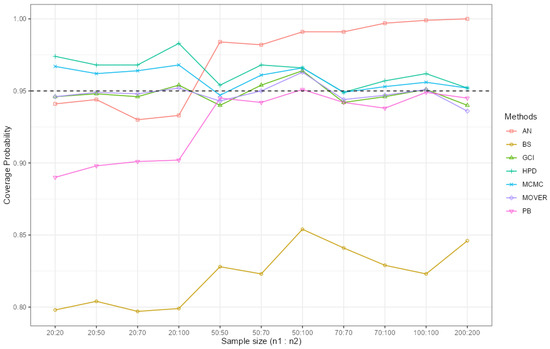
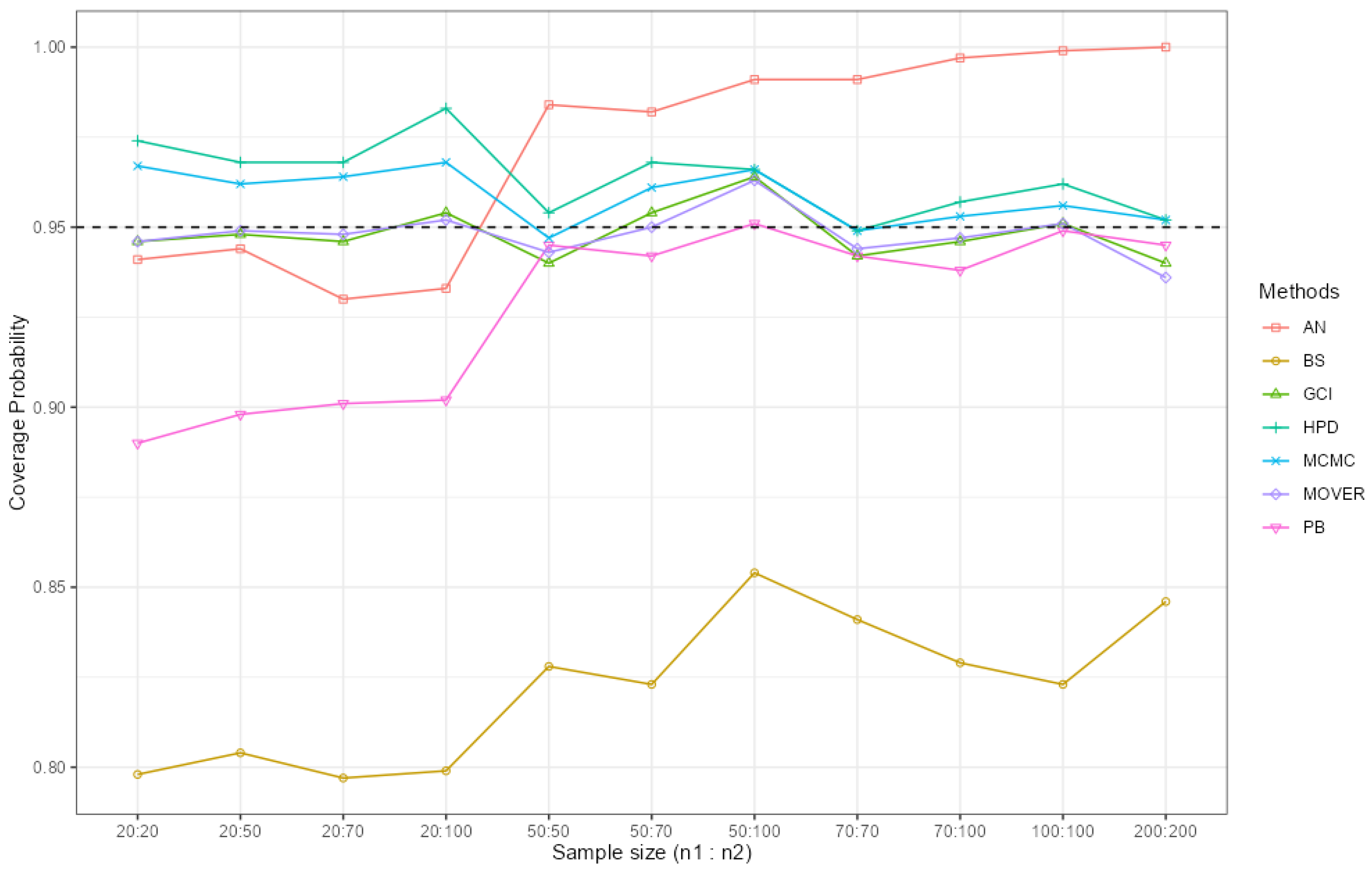
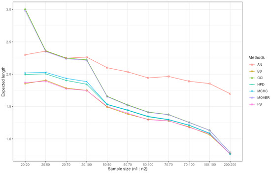
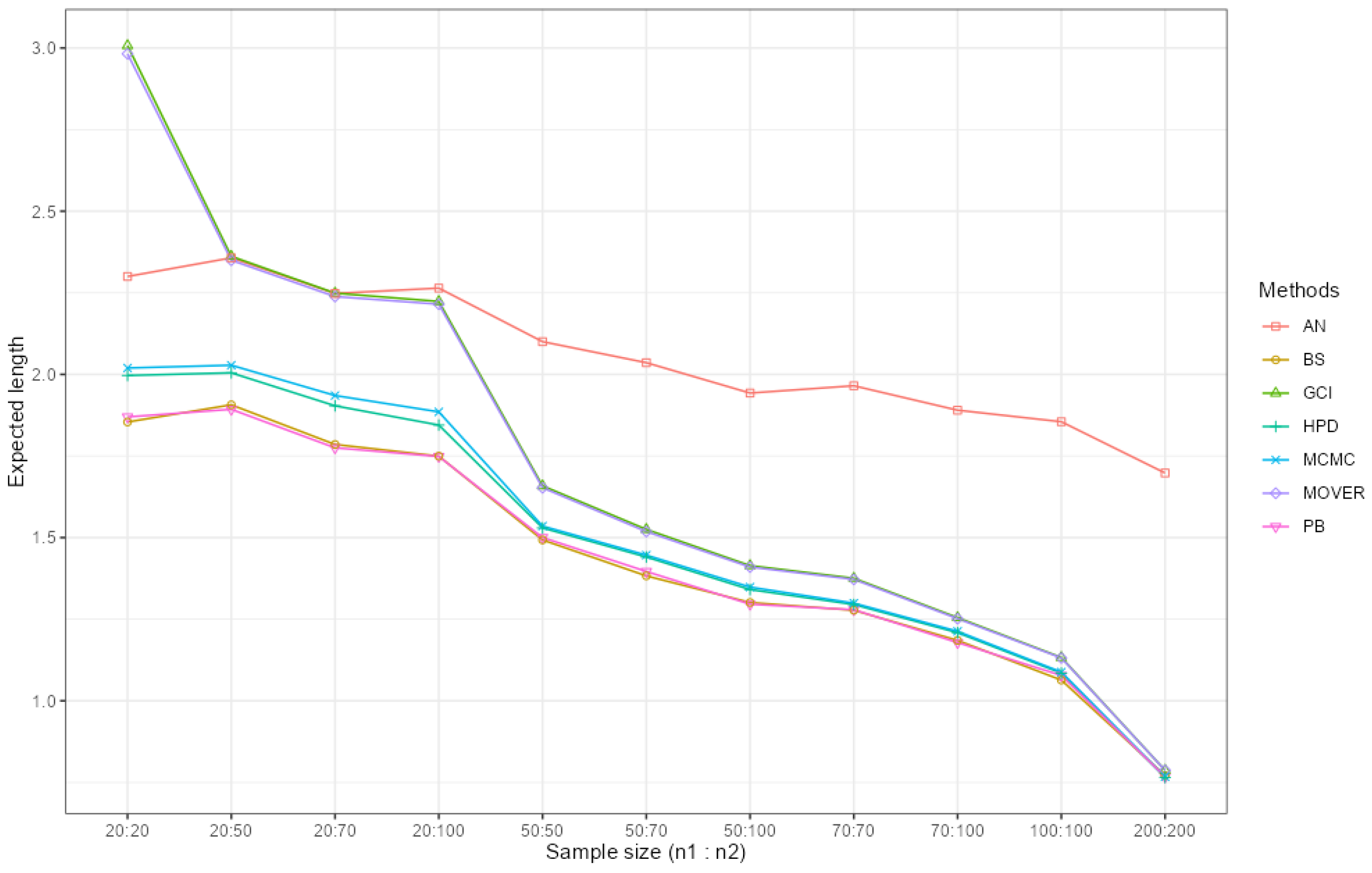
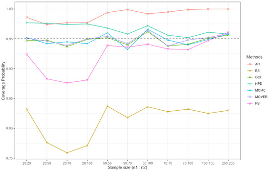
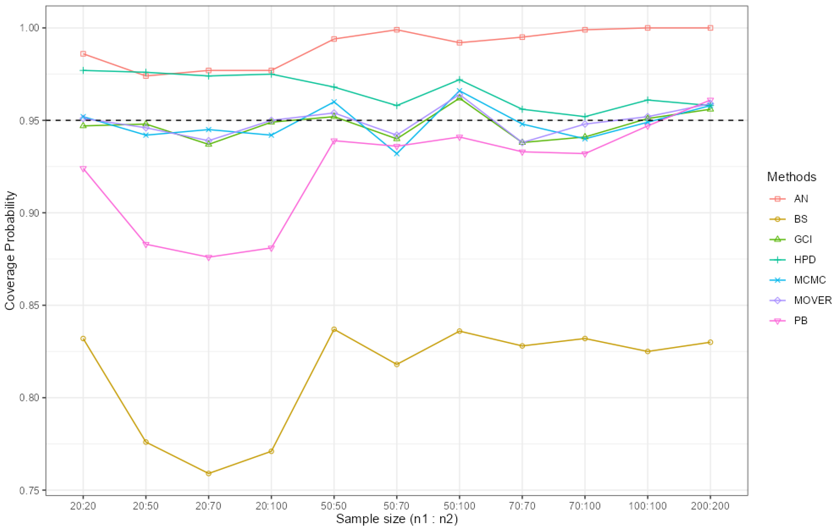
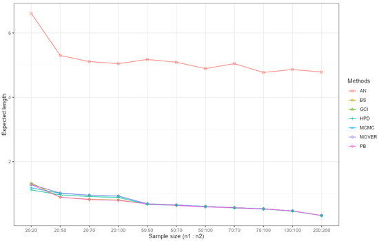
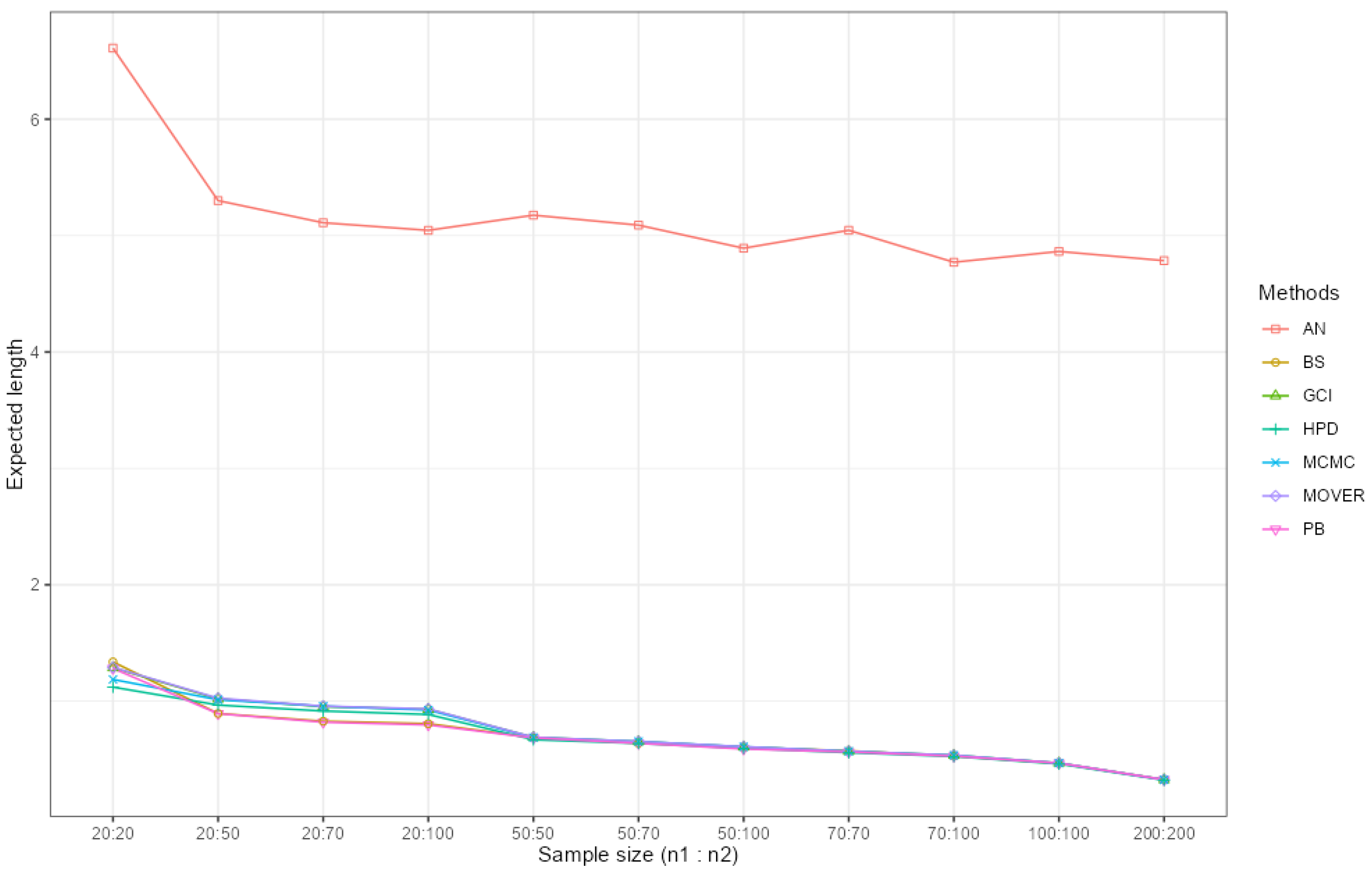
Based on the simulation study, the performance of the 95% confidence intervals for the variance difference under the $ZITR$ distribution was evaluated in terms of coverage probability (CP) and expected length (EL), as presented in Table 1, Table 2 and Table 3, with the corresponding graphical results illustrated in Figure 1 and Figure 2. Overall, the results indicate that the Bayesian HPD method provides a good balance between coverage and interval length, maintaining nominal coverage while yielding relatively short intervals.

Table 1. CP and EL for 95% confidence intervals for the difference between two variances of $ZITR$ when $({\mu }_1,{\mu }_2)=(0.5,0.5)$, $({\lambda }_1,{\lambda }_2)=(0.2,0.2)$, and $({\delta }_1,{\delta }_2)=(0.1,0.1),(0.1,0.3),(0.3,0.3)$.

$\mathit{\delta }$	Coverage Probability
	n	PB	BS	GCI	MOVER	AN	MCMC	HPD
0.1:0.1	20:20	0.890	0.798	0.946	0.946	0.941	0.967	0.974
		(1.8697)	(1.8541)	(3.0073)	(2.9821)	(2.3000)	(2.0196)	(1.9967)
	20:50	0.898	0.804	0.948	0.949	0.944	0.962	0.968
		(1.8930)	(1.9068)	(2.3617)	(2.3497)	(2.3570)	(2.0281)	(2.0047)
	20:70	0.901	0.797	0.946	0.948	0.930	0.964	0.968
		(1.7750)	(1.7854)	(2.2490)	(2.2385)	(2.2481)	(1.9353)	(1.9037)
	20:100	0.902	0.799	0.954	0.952	0.933	0.968	0.983
		(1.7485)	(1.7496)	(2.2235)	(2.2150)	(2.2643)	(1.8852)	(1.8448)
	50:50	0.945	0.828	0.940	0.943	0.984	0.947	0.954
		(1.5002)	(1.4928)	(1.6585)	(1.6527)	(2.1003)	(1.5352)	(1.5297)
	50:70	0.942	0.823	0.954	0.950	0.982	0.961	0.968
		(1.3963)	(1.3828)	(1.5251)	(1.5184)	(2.0359)	(1.4463)	(1.4406)
	50:100	0.951	0.854	0.964	0.963	0.991	0.966	0.966
		(1.2959)	(1.3012)	(1.4141)	(1.4098)	(1.9428)	(1.3483)	(1.3408)
	70:70	0.942	0.841	0.942	0.944	0.991	0.949	0.949
		(1.2791)	(1.2774)	(1.3755)	(1.3720)	(1.9651)	(1.2992)	(1.2950)
	70:100	0.938	0.829	0.946	0.947	0.997	0.953	0.957
		(1.1784)	(1.1851)	(1.2548)	(1.2517)	(1.8903)	(1.2129)	(1.2087)
	100:100	0.949	0.823	0.951	0.951	0.999	0.956	0.962
		(1.0776)	(1.0635)	(1.1328)	(1.1314)	(1.8550)	(1.0880)	(1.0848)
	200:200	0.945	0.846	0.940	0.936	1.000	0.952	0.952
		(0.7674)	(0.7709)	(0.7872)	(0.7871)	(1.6979)	(0.7674)	(0.7653)
0.1:0.3	20:20	0.940	0.848	0.955	0.955	0.980	0.940	0.947
		(2.4178)	(2.4070)	(3.3615)	(3.3347)	(3.3853)	(2.6985)	(2.6750)
	20:50	0.936	0.846	0.958	0.956	0.999	0.959	0.973
		(2.0098)	(2.0110)	(2.5138)	(2.5001)	(3.2709)	(2.1640)	(2.1452)
	20:70	0.901	0.799	0.953	0.949	0.999	0.953	0.959
		(1.8845)	(1.8643)	(2.3650)	(2.3527)	(3.3024)	(2.0308)	(2.0057)
	20:100	0.905	0.801	0.957	0.957	0.999	0.961	0.973
		(1.7812)	(1.7721)	(2.2542)	(2.2462)	(3.2407)	(1.9317)	(1.8986)
	50:50	0.935	0.845	0.950	0.950	0.998	0.936	0.942
		(1.6166)	(1.6279)	(1.8148)	(1.8098)	(3.1311)	(1.6959)	(1.6884)
	50:70	0.947	0.826	0.952	0.951	1.000	0.951	0.956
		(1.4871)	(1.5049)	(1.6438)	(1.6399)	(3.0830)	(1.5561)	(1.5506)
	50:100	0.954	0.838	0.963	0.964	1.000	0.964	0.966
		(1.3727)	(1.3593)	(1.4853)	(1.4833)	(3.0340)	(1.4179)	(1.4118)
	70:70	0.938	0.847	0.945	0.944	0.999	0.946	0.950
		(1.3662)	(1.3828)	(1.4883)	(1.4862)	(3.0070)	(1.4262)	(1.4207)
	70:100	0.945	0.823	0.950	0.954	1.000	0.954	0.958
		(1.2547)	(1.2460)	(1.3443)	(1.3414)	(2.9930)	(1.2987)	(1.2946)
	100:100	0.948	0.827	0.946	0.950	1.000	0.947	0.948
		(1.1594)	(1.1792)	(1.2242)	(1.2222)	(2.9635)	(1.1914)	(1.1874)
	200:200	0.945	0.854	0.954	0.952	1.000	0.953	0.952
		(0.8234)	(0.8340)	(0.8461)	(0.8451)	(2.8313)	(0.8350)	(0.8326)
0.3:0.3	20:20	0.942	0.823	0.954	0.954	0.995	0.951	0.966
		(2.5712)	(2.6018)	(3.6391)	(3.6100)	(3.9938)	(2.8824)	(2.8585)
	20:50	0.911	0.812	0.954	0.951	0.997	0.951	0.958
		(2.1774)	(2.1700)	(2.8987)	(2.8862)	(3.9748)	(2.4190)	(2.3811)
	20:70	0.910	0.806	0.962	0.961	0.994	0.950	0.953
		(2.0972)	(2.0901)	(2.8033)	(2.7886)	(3.9818)	(2.3236)	(2.2722)
	20:100	0.887	0.786	0.959	0.956	0.996	0.949	0.942
		(1.9726)	(1.9846)	(2.6467)	(2.6367)	(3.9361)	(2.1958)	(2.1379)
	50:50	0.945	0.830	0.952	0.953	1.000	0.948	0.959
		(1.7255)	(1.7371)	(1.9664)	(1.9593)	(3.8686)	(1.8176)	(1.8101)
	50:70	0.956	0.832	0.959	0.959	1.000	0.957	0.963
		(1.6112)	(1.6173)	(1.7946)	(1.7892)	(3.8690)	(1.6868)	(1.6791)
	50:100	0.950	0.835	0.962	0.965	1.000	0.960	0.960
		(1.4968)	(1.5082)	(1.6585)	(1.6529)	(3.8057)	(1.5651)	(1.5546)
	70:70	0.950	0.836	0.950	0.950	1.000	0.946	0.951
		(1.4698)	(1.4649)	(1.6093)	(1.6058)	(3.8379)	(1.5294)	(1.5239)
	70:100	0.944	0.834	0.947	0.945	1.000	0.947	0.949
		(1.3465)	(1.3127)	(1.4567)	(1.4530)	(3.7813)	(1.4008)	(1.3950)
	100:100	0.940	0.826	0.946	0.948	1.000	0.942	0.947
		(1.2338)	(1.2004)	(1.3157)	(1.3150)	(3.7572)	(1.2739)	(1.2698)
	200:200	0.943	0.825	0.945	0.947	1.000	0.947	0.946
		(0.8781)	(0.8749)	(0.9071)	(0.9070)	(3.6713)	(0.8929)	(0.8903)

The boldfaced numerical entries denote the smallest expected interval lengths among the methods with coverage probabilities not less than the nominal confidence level.

Table 2. CP and EL for 95% confidence intervals for the difference between two variances of $ZITR$ when $({\mu }_1,{\mu }_2)=(0.5,0.5)$, $({\lambda }_1,{\lambda }_2)=(0.2,1)$, and $({\delta }_1,{\delta }_2)=(0.1,0.1),(0.1,0.3),(0.3,0.3)$.

$\mathit{\delta }$	Coverage Probability
	n	PB	BS	GCI	MOVER	AN	MCMC	HPD
0.1:0.1	20:20	0.889	0.769	0.970	0.969	0.824	0.971	0.962
		(1.6072)	(1.6154)	(2.1014)	(2.0984)	(1.8003)	(1.7370)	(1.6835)
	20:50	0.863	0.754	0.954	0.956	0.822	0.965	0.963
		(1.5663)	(1.5309)	(2.0524)	(2.0507)	(1.8456)	(1.7120)	(1.6485)
	20:70	0.856	0.753	0.956	0.956	0.798	0.969	0.969
		(1.5327)	(1.5728)	(2.0163)	(2.0158)	(1.7670)	(1.6914)	(1.6261)
	20:100	0.844	0.727	0.944	0.943	0.811	0.948	0.956
		(1.5382)	(1.5377)	(2.0320)	(2.0307)	(1.7944)	(1.6938)	(1.6266)
	50:50	0.920	0.804	0.949	0.948	0.917	0.961	0.956
		(1.0796)	(1.0909)	(1.1927)	(1.1925)	(1.5153)	(1.1146)	(1.0960)
	50:70	0.903	0.796	0.940	0.939	0.910	0.945	0.945
		(1.0840)	(1.0927)	(1.1857)	(1.1850)	(1.5193)	(1.1195)	(1.1004)
	50:100	0.917	0.794	0.951	0.951	0.914	0.957	0.959
		(1.0723)	(1.0681)	(1.1775)	(1.1772)	(1.5083)	(1.1110)	(1.0913)
	70:70	0.938	0.816	0.954	0.952	0.932	0.961	0.964
		(0.9312)	(0.9397)	(0.9922)	(0.9914)	(1.4186)	(0.9468)	(0.9349)
	70:100	0.922	0.791	0.953	0.955	0.931	0.958	0.956
		(0.9177)	(0.8985)	(0.9769)	(0.9773)	(1.4014)	(0.9417)	(0.9292)
	100:100	0.929	0.825	0.953	0.952	0.968	0.952	0.952
		(0.7887)	(0.7909)	(0.8244)	(0.8245)	(1.3567)	(0.7960)	(0.7881)
	200:200	0.951	0.838	0.949	0.950	0.991	0.952	0.951
		(0.5576)	(0.5583)	(0.5710)	(0.5711)	(1.2434)	(0.5605)	(0.5570)
0.1:0.3	20:20	0.871	0.770	0.946	0.945	0.868	0.961	0.970
		(1.6143)	(1.6232)	(2.1198)	(2.1189)	(1.9919)	(1.7795)	(1.7345)
	20:50	0.871	0.768	0.959	0.958	0.865	0.972	0.970
		(1.5640)	(1.5808)	(2.0479)	(2.0456)	(1.9636)	(1.7123)	(1.6517)
	20:70	0.831	0.732	0.943	0.943	0.842	0.961	0.965
		(1.5391)	(1.5354)	(2.0349)	(2.0339)	(1.9740)	(1.7016)	(1.6355)
	20:100	0.831	0.732	0.943	0.943	0.842	0.961	0.965
		(1.5391)	(1.5354)	(2.0349)	(2.0339)	(1.9740)	(1.7016)	(1.6355)
	50:50	0.909	0.797	0.939	0.938	0.956	0.949	0.954
		(1.0986)	(1.0974)	(1.2042)	(1.2040)	(1.7119)	(1.1392)	(1.1226)
	50:70	0.919	0.816	0.954	0.953	0.943	0.964	0.960
		(1.0698)	(1.0772)	(1.1816)	(1.1818)	(1.6622)	(1.1173)	(1.0993)
	50:100	0.915	0.781	0.955	0.955	0.954	0.960	0.965
		(1.0737)	(1.0550)	(1.1805)	(1.1802)	(1.6732)	(1.1141)	(1.0950)
	70:70	0.926	0.802	0.952	0.951	0.971	0.953	0.956
		(0.9317)	(0.9317)	(0.9991)	(0.9987)	(1.6229)	(0.9634)	(0.9520)
	70:100	0.929	0.811	0.951	0.951	0.973	0.952	0.954
		(0.9225)	(0.9264)	(0.9839)	(0.9848)	(1.6016)	(0.9482)	(0.9360)
	100:100	0.935	0.818	0.951	0.952	0.988	0.950	0.956
		(0.7909)	(0.7876)	(0.8310)	(0.8310)	(1.5297)	(0.8098)	(0.8023)
	200:200	0.934	0.805	0.945	0.947	0.997	0.950	0.949
		(0.5605)	(0.5575)	(0.5753)	(0.5752)	(1.4328)	(0.5692)	(0.5659)
0.3:0.3	20:20	0.866	0.773	0.956	0.955	0.942	0.943	0.931
		(1.8684)	(1.8636)	(2.5855)	(2.5839)	(2.9839)	(2.0867)	(2.0101)
	20:50	0.854	0.750	0.954	0.953	0.923	0.941	0.927
		(1.7983)	(1.8050)	(2.5109)	(2.5082)	(2.9599)	(2.0243)	(1.9313)
	20:70	0.833	0.738	0.952	0.952	0.927	0.938	0.918
		(1.7813)	(1.8093)	(2.4759)	(2.4749)	(2.9853)	(2.0017)	(1.9077)
	20:100	0.836	0.726	0.957	0.958	0.915	0.934	0.906
		(1.7724)	(1.7688)	(2.4441)	(2.4436)	(2.9267)	(1.9735)	(1.8775)
	50:50	0.917	0.816	0.964	0.962	0.998	0.955	0.944
		(1.2268)	(1.2387)	(1.3997)	(1.4001)	(2.8355)	(1.3043)	(1.2795)
	50:70	0.920	0.836	0.959	0.958	0.998	0.951	0.944
		(1.2336)	(1.2308)	(1.3995)	(1.3995)	(2.8659)	(1.3087)	(1.2821)
	50:100	0.913	0.799	0.946	0.947	0.993	0.949	0.941
		(1.2325)	(1.2344)	(1.3867)	(1.3864)	(2.8508)	(1.2947)	(1.2672)
	70:70	0.937	0.827	0.964	0.965	0.999	0.956	0.946
		(1.0665)	(1.0738)	(1.1614)	(1.1610)	(2.8198)	(1.1102)	(1.0935)
	70:100	0.917	0.798	0.935	0.932	0.999	0.933	0.932
		(1.0540)	(1.0538)	(1.1392)	(1.1392)	(2.7861)	(1.0906)	(1.0737)
	100:100	0.928	0.817	0.950	0.952	1.000	0.945	0.935
		(0.8914)	(0.8848)	(0.9427)	(0.9428)	(2.7395)	(0.9153)	(0.9053)
	200:200	0.935	0.822	0.943	0.941	1.000	0.944	0.938
		(0.6354)	(0.6392)	(0.6559)	(0.6555)	(2.6865)	(0.6490)	(0.6446)

The boldfaced numerical entries denote the smallest expected interval lengths among the methods with coverage probabilities not less than the nominal confidence level.

Table 3. CP and EL for 95% confidence intervals for the difference between two variances of $ZITR$ when $({\mu }_1,{\mu }_2)=(0.5,0.5)$, $({\lambda }_1,{\lambda }_2)=(1,1)$, and $({\delta }_1,{\delta }_2)=(0.1,0.1),(0.1,0.3),(0.3,0.3)$.

$\mathit{\delta }$	Coverage Probability
	n	PB	BS	GCI	MOVER	AN	MCMC	HPD
0.1:0.1	20:20	0.933	0.819	0.951	0.952	0.978	0.977	0.987
		(0.5729)	(0.5738)	(0.6970)	(0.6925)	(0.7100)	(0.6563)	(0.6529)
	20:50	0.911	0.814	0.938	0.939	0.951	0.971	0.980
		(0.4973)	(0.4939)	(0.5742)	(0.5713)	(0.6853)	(0.5615)	(0.5547)
	20:70	0.903	0.815	0.940	0.941	0.942	0.957	0.975
		(0.4749)	(0.4788)	(0.5515)	(0.5489)	(0.6633)	(0.5393)	(0.5306)
	20:100	0.887	0.778	0.931	0.931	0.923	0.954	0.974
		(0.4510)	(0.4421)	(0.5260)	(0.5241)	(0.6499)	(0.5165)	(0.5061)
	50:50	0.942	0.844	0.949	0.949	0.996	0.964	0.969
		(0.3964)	(0.3993)	(0.4182)	(0.4167)	(0.6319)	(0.3998)	(0.3986)
	50:70	0.931	0.843	0.944	0.944	0.993	0.959	0.965
		(0.3687)	(0.3692)	(0.3871)	(0.3859)	(0.6079)	(0.3828)	(0.3814)
	50:100	0.963	0.831	0.964	0.965	0.992	0.977	0.981
		(0.3456)	(0.3374)	(0.3605)	(0.3598)	(0.5920)	(0.3563)	(0.3546)
	70:70	0.937	0.831	0.939	0.940	0.997	0.954	0.960
		(0.3373)	(0.3369)	(0.3493)	(0.3482)	(0.5851)	(0.3349)	(0.3340)
	70:100	0.939	0.830	0.946	0.946	0.992	0.957	0.961
		(0.3123)	(0.3072)	(0.3214)	(0.3207)	(0.5664)	(0.3176)	(0.3165)
	100:100	0.945	0.821	0.952	0.951	0.998	0.956	0.957
		(0.2847)	(0.2868)	(0.2911)	(0.2906)	(0.5471)	(0.2795)	(0.2787)
	200:200	0.957	0.845	0.959	0.959	1.000	0.959	0.959
		(0.2030)	(0.1997)	(0.2053)	(0.2050)	(0.5065)	(0.1987)	(0.1981)
0.1:0.3	20:20	0.934	0.811	0.948	0.945	0.982	0.954	0.960
		(0.6168)	(0.6115)	(0.7795)	(0.7770)	(1.0019)	(0.7436)	(0.7377)
	20:50	0.904	0.804	0.943	0.941	1.000	0.947	0.971
		(0.5093)	(0.5089)	(0.5961)	(0.5944)	(0.9918)	(0.5853)	(0.5798)
	20:70	0.898	0.796	0.939	0.942	1.000	0.950	0.970
		(0.4745)	(0.4767)	(0.5545)	(0.5523)	(0.9641)	(0.5475)	(0.5402)
	20:100	0.898	0.808	0.952	0.951	1.000	0.953	0.969
		(0.4602)	(0.4639)	(0.5357)	(0.5336)	(0.9753)	(0.5251)	(0.5158)
	50:50	0.951	0.840	0.957	0.954	0.997	0.963	0.966
		(0.4104)	(0.4093)	(0.4416)	(0.4410)	(0.9406)	(0.4382)	(0.4366)
	50:70	0.940	0.826	0.949	0.951	1.000	0.944	0.950
		(0.3801)	(0.3762)	(0.4035)	(0.4026)	(0.9400)	(0.4000)	(0.3986)
	50:100	0.951	0.843	0.958	0.955	1.000	0.955	0.964
		(0.3528)	(0.3606)	(0.3700)	(0.3698)	(0.9309)	(0.3673)	(0.3657)
	70:70	0.940	0.832	0.942	0.942	0.999	0.949	0.950
		(0.3486)	(0.3553)	(0.3684)	(0.3684)	(0.9190)	(0.3661)	(0.3649)
	70:100	0.941	0.830	0.944	0.944	1.000	0.942	0.949
		(0.3231)	(0.3200)	(0.3355)	(0.3351)	(0.9146)	(0.3326)	(0.3316)
	100:100	0.955	0.843	0.957	0.955	1.000	0.956	0.960
		(0.2953)	(0.2923)	(0.3048)	(0.3044)	(0.9023)	(0.3027)	(0.3019)
	200:200	0.949	0.834	0.953	0.954	1.000	0.953	0.956
		(0.2096)	(0.2085)	(0.2132)	(0.2132)	(0.8647)	(0.2115)	(0.2110)
0.3:0.3	20:20	0.949	0.828	0.957	0.950	0.998	0.977	0.986
		(0.6528)	(0.6365)	(0.8505)	(0.8479)	(1.2132)	(0.7976)	(0.7920)
	20:50	0.923	0.831	0.951	0.949	0.998	0.971	0.982
		(0.5440)	(0.5467)	(0.6740)	(0.6736)	(1.1939)	(0.6509)	(0.6399)
	20:70	0.924	0.806	0.955	0.955	0.998	0.968	0.974
		(0.5309)	(0.5319)	(0.6531)	(0.6529)	(1.1951)	(0.6269)	(0.6127)
	20:100	0.904	0.799	0.951	0.948	0.998	0.976	0.977
		(0.5044)	(0.5025)	(0.6288)	(0.6285)	(1.1852)	(0.6025)	(0.5860)
	50:50	0.952	0.848	0.958	0.958	1.000	0.963	0.970
		(0.4260)	(0.4186)	(0.4663)	(0.4667)	(1.1804)	(0.4605)	(0.4588)
	50:70	0.940	0.825	0.947	0.946	1.000	0.958	0.961
		(0.3951)	(0.3883)	(0.4285)	(0.4284)	(1.1800)	(0.4271)	(0.4253)
	50:100	0.935	0.838	0.945	0.944	1.000	0.959	0.962
		(0.3715)	(0.3746)	(0.3989)	(0.3985)	(1.1704)	(0.3975)	(0.3952)
	70:70	0.928	0.819	0.931	0.937	1.000	0.938	0.947
		(0.3660)	(0.3642)	(0.3898)	(0.3895)	(1.1735)	(0.3853)	(0.3840)
	70:100	0.949	0.842	0.958	0.953	1.000	0.960	0.967
		(0.3334)	(0.3318)	(0.3529)	(0.3532)	(1.1563)	(0.3523)	(0.3509)
	100:100	0.945	0.840	0.951	0.947	1.000	0.954	0.962
		(0.3043)	(0.3029)	(0.3182)	(0.3183)	(1.1504)	(0.3151)	(0.3142)
	200:200	0.937	0.839	0.935	0.935	1.000	0.936	0.939
		(0.2173)	(0.2183)	(0.2218)	(0.2216)	(1.1189)	(0.2191)	(0.2185)

The boldfaced numerical entries denote the smallest expected interval lengths among the methods with coverage probabilities not less than the nominal confidence level.

Figure 1. The coverage probabilities (CPs) for the confidence intervals of the difference in variances under the $ZITR$ distribution were evaluated for the parameter setting $\left({\mu }_1,{\mu }_2\right)=(0.5,0.5)$, $\left({\lambda }_1,{\lambda }_2\right)=(0.2,0.2)$, and $\left({\delta }_1,{\delta }_2\right)=(0.1,0.1)$. Several methods were considered, and a method was regarded as satisfactory if its CP was at least $0.95$, which corresponds to the nominal confidence level that is represented by the dashed line in the figure, indicating adequate coverage of the true parameter. The results in the table show that the AN, MCMC, and HPD methods consistently produced CP values that were close to or exceeded the nominal level, suggesting that these approaches provide reliable interval estimation for this scenario.

Figure 2. The expected lengths (ELs) of the confidence intervals for the difference in variances under the $ZITR$ distribution were examined for the parameter configuration $\left({\mu }_1,{\mu }_2\right)=(0.5,0.5)$, $\left({\lambda }_1,{\lambda }_2\right)=(0.2,0.2)$, and $\left({\delta }_1,{\delta }_2\right)=(0.1,0.1)$. The assessment focused on methods that achieved coverage probabilities (CPs) close to or exceeding the nominal confidence level of 0.95, while also yielding the shortest interval lengths. From this setting, the AN, MCMC, and HPD methods satisfied the CP criterion. Among these, the HPD approach produced the smallest expected length, indicating a more efficient interval estimate under the given conditions.

The Bayesian MCMC, Bayesian HPD, GCI, and MOVER methods achieved coverage probabilities close to or above the nominal level of 0.95 across most of the scenarios. In contrast, the PB and AN methods showed improved coverage as the sample sizes increased, performing more satisfactorily in the larger samples.

In terms of interval precision, measured by expected length, the PB and BS methods produced the shortest intervals. However, their coverage probabilities fell below the nominal level in several cases, and they were therefore not considered further. Among the methods that met the coverage criterion, the Bayesian HPD method consistently yielded the shortest expected lengths, indicating greater efficiency.

The coverage probabilities and expected interval lengths of the 95% confidence intervals for the ratio variances under the $ZITR$ distribution are presented in Table 4, Table 5 and Table 6, with the corresponding graphical results illustrated in Figure 3 and Figure 4. Similar patterns were observed for both the variance difference and the variance ratio, and the main conclusions remained consistent across the two settings.

Table 4. Coverage probability (CP) and expected length (EL) of 95% confidence intervals for the ratio of two variances of $ZITR$ when $({\mu }_1,{\mu }_2)=(0.5,0.5)$, $({\lambda }_1,{\lambda }_2)=(0.2,0.2)$, and $({\delta }_1,{\delta }_2)=(0.1,0.1),(0.1,0.3),(0.3,0.3)$.

$\mathit{\delta }$	Coverage Probability
	n	PB	BS	GCI	MOVER	AN	MCMC	HPD
0.1:0.1	20:20	0.926	0.865	0.946	0.946	0.951	0.959	0.953
		(2.3133)	(2.3674)	(2.1306)	(2.1305)	(2.7186)	(1.6255)	(1.5268)
	20:50	0.898	0.796	0.948	0.949	0.937	0.962	0.958
		(1.3898)	(1.4129)	(1.5884)	(1.5990)	(2.1751)	(1.3310)	(1.2629)
	20:70	0.901	0.783	0.946	0.948	0.940	0.964	0.962
		(1.2672)	(1.2824)	(1.5239)	(1.5336)	(2.0341)	(1.2861)	(1.2230)
	20:100	0.902	0.786	0.954	0.952	0.933	0.968	0.977
		(1.2108)	(1.2162)	(1.4929)	(1.5029)	(2.0237)	(1.2490)	(1.1911)
	50:50	0.945	0.834	0.940	0.943	0.979	0.947	0.947
		(1.1545)	(1.1566)	(1.1223)	(1.1223)	(2.1047)	(1.0119)	(0.9807)
	50:70	0.942	0.818	0.954	0.950	0.984	0.961	0.958
		(1.0176)	(1.0196)	(1.0247)	(1.0248)	(1.9632)	(0.9540)	(0.9269)
	50:100	0.951	0.834	0.964	0.963	0.981	0.966	0.964
		(0.9148)	(0.9218)	(0.9517)	(0.9536)	(1.8834)	(0.8960)	(0.8726)
	70:70	0.942	0.846	0.942	0.944	0.991	0.949	0.950
		(0.9386)	(0.9417)	(0.9254)	(0.9250)	(1.9042)	(0.8542)	(0.8340)
	70:100	0.938	0.836	0.946	0.947	0.985	0.953	0.951
		(0.8307)	(0.8367)	(0.8383)	(0.8386)	(1.8718)	(0.7987)	(0.7814)
	100:100	0.949	0.826	0.951	0.951	0.994	0.956	0.956
		(0.7578)	(0.7492)	(0.7491)	(0.7499)	(1.8641)	(0.7085)	(0.6958)
	200:200	0.946	0.852	0.940	0.936	0.998	0.952	0.950
		(0.5254)	(0.5289)	(0.5234)	(0.5234)	(1.7388)	(0.5048)	(0.4995)
0.1:0.3	20:20	0.930	0.846	0.954	0.953	0.949	0.940	0.964
		(1.3857)	(1.4147)	(1.4766)	(1.4764)	(2.9845)	(1.3116)	(1.2380)
	20:50	0.918	0.806	0.957	0.955	0.918	0.963	0.975
		(0.9756)	(0.9839)	(1.1757)	(1.1816)	(2.3373)	(1.0405)	(0.9903)
	20:70	0.884	0.756	0.949	0.952	0.918	0.956	0.956
		(0.8926)	(0.8888)	(1.1090)	(1.1135)	(2.2047)	(0.9647)	(0.9200)
	20:100	0.890	0.781	0.960	0.958	0.885	0.965	0.966
		(0.8464)	(0.8505)	(1.0697)	(1.0750)	(2.0340)	(0.9222)	(0.8811)
	50:50	0.942	0.841	0.951	0.956	0.913	0.940	0.955
		(0.7626)	(0.7700)	(0.7857)	(0.7853)	(2.1805)	(0.7703)	(0.7493)
	50:70	0.948	0.827	0.955	0.953	0.896	0.955	0.967
		(0.6888)	(0.7011)	(0.7266)	(0.7266)	(2.0487)	(0.7084)	(0.6905)
	50:100	0.943	0.822	0.960	0.961	0.891	0.961	0.965
		(0.6252)	(0.6223)	(0.6624)	(0.6635)	(1.9431)	(0.6433)	(0.6280)
	70:70	0.938	0.847	0.945	0.947	0.904	0.949	0.952
		(0.6203)	(0.6291)	(0.6367)	(0.6366)	(1.9793)	(0.6320)	(0.6188)
	70:100	0.940	0.815	0.950	0.947	0.900	0.948	0.960
		(0.5704)	(0.5687)	(0.5915)	(0.5912)	(1.8855)	(0.5836)	(0.5723)
	100:100	0.945	0.834	0.948	0.948	0.914	0.946	0.955
		(0.5202)	(0.5314)	(0.5276)	(0.5274)	(1.8782)	(0.5262)	(0.5181)
	200:200	0.945	0.843	0.950	0.948	0.927	0.950	0.953
		(0.3561)	(0.3597)	(0.3590)	(0.3588)	(1.7522)	(0.3588)	(0.3556)
0.3:0.3	20:20	0.942	0.855	0.954	0.954	0.997	0.951	0.959
		(1.7159)	(1.8086)	(1.8804)	(1.8868)	(5.4840)	(1.5829)	(1.4886)
	20:50	0.911	0.804	0.954	0.951	0.996	0.951	0.936
		(1.1647)	(1.1688)	(1.4468)	(1.4569)	(4.2976)	(1.2259)	(1.1600)
	20:70	0.910	0.796	0.962	0.961	0.993	0.950	0.936
		(1.0934)	(1.0926)	(1.4018)	(1.4100)	(3.9692)	(1.1728)	(1.1098)
	20:100	0.887	0.774	0.959	0.956	0.991	0.949	0.923
		(0.9936)	(0.9986)	(1.3038)	(1.3108)	(3.7809)	(1.0853)	(1.0288)
	50:50	0.945	0.843	0.952	0.953	0.999	0.948	0.949
		(0.9436)	(0.9550)	(0.9745)	(0.9754)	(4.1058)	(0.9270)	(0.9023)
	50:70	0.956	0.829	0.959	0.959	1.000	0.957	0.950
		(0.8332)	(0.8396)	(0.8740)	(0.8749)	(3.9598)	(0.8361)	(0.8149)
	50:100	0.950	0.821	0.962	0.965	0.999	0.960	0.948
		(0.7652)	(0.7739)	(0.8186)	(0.8196)	(3.9290)	(0.7797)	(0.7604)
	70:70	0.950	0.831	0.950	0.950	1.000	0.946	0.948
		(0.7763)	(0.7745)	(0.7944)	(0.7950)	(3.9938)	(0.7699)	(0.7545)
	70:100	0.943	0.834	0.947	0.945	1.000	0.947	0.945
		(0.6913)	(0.6776)	(0.7171)	(0.7178)	(4.0195)	(0.6978)	(0.6844)
	100:100	0.940	0.824	0.946	0.948	1.000	0.942	0.947
		(0.6385)	(0.6214)	(0.6497)	(0.6504)	(3.9838)	(0.6373)	(0.6277)
	200:200	0.943	0.824	0.945	0.947	1.000	0.947	0.952
		(0.4434)	(0.4432)	(0.4478)	(0.4481)	(3.9113)	(0.4437)	(0.4398)

The boldfaced numerical entries denote the smallest expected interval lengths among the methods with coverage probabilities not less than the nominal confidence level.

Table 5. Coverage probability (CP) and expected length (EL) of 95% confidence intervals for the ratio of two variances of $ZITR$ when $({\mu }_1,{\mu }_2)=(0.5,0.5)$, $({\lambda }_1,{\lambda }_2)=(0.2,1)$, and $({\delta }_1,{\delta }_2)=(0.1,0.1),(0.1,0.3),(0.3,0.3)$.

$\mathit{\delta }$	Coverage Probability
	n	PB	BS	GCI	MOVER	AN	MCMC	HPD
0.1:0.1	20:20	0.928	0.861	0.957	0.961	0.948	0.964	0.932
		(10.8528)	(11.3711)	(9.4251)	(9.4855)	(13.1279)	(6.0397)	(5.6461)
	20:50	0.908	0.791	0.951	0.950	0.914	0.963	0.948
		(6.3288)	(6.2282)	(7.1640)	(7.2365)	(10.5652)	(5.5712)	(5.2687)
	20:70	0.921	0.793	0.964	0.961	0.898	0.972	0.963
		(5.5040)	(5.5999)	(6.5613)	(6.6304)	(10.1635)	(5.2871)	(5.0180)
	20:100	0.893	0.755	0.944	0.943	0.906	0.958	0.952
		(5.1249)	(5.1118)	(6.3247)	(6.3765)	(9.9624)	(5.1465)	(4.8981)
	50:50	0.946	0.850	0.952	0.953	0.957	0.959	0.949
		(5.2476)	(5.3728)	(5.0183)	(5.0320)	(10.0571)	(4.1581)	(4.0117)
	50:70	0.924	0.824	0.926	0.928	0.943	0.949	0.938
		(4.5621)	(4.6110)	(4.5536)	(4.5619)	(9.6611)	(4.0171)	(3.8913)
	50:100	0.950	0.830	0.958	0.962	0.939	0.967	0.964
		(4.0225)	(3.9867)	(4.1405)	(4.1567)	(9.2330)	(3.7579)	(3.6509)
	70:70	0.948	0.841	0.946	0.948	0.947	0.954	0.939
		(4.2014)	(4.2289)	(4.0677)	(4.0768)	(9.5088)	(3.5541)	(3.4575)
	70:100	0.931	0.800	0.937	0.941	0.940	0.945	0.935
		(3.6473)	(3.5783)	(3.6428)	(3.6549)	(9.2202)	(3.3462)	(3.2651)
	100:100	0.947	0.845	0.949	0.951	0.962	0.947	0.940
		(3.4006)	(3.3852)	(3.3289)	(3.3341)	(9.1634)	(2.9890)	(2.9282)
	200:200	0.948	0.821	0.956	0.955	0.975	0.951	0.946
		(2.2864)	(2.3125)	(2.2730)	(2.2731)	(8.6120)	(2.1377)	(2.1115)
0.1:0.3	20:20	0.935	0.832	0.957	0.957	0.879	0.978	0.973
		(5.0182)	(5.2784)	(5.3722)	(5.4109)	(14.7933)	(4.2908)	(4.0446)
	20:50	0.904	0.799	0.957	0.960	0.782	0.966	0.962
		(3.4222)	(3.4679)	(4.2240)	(4.2513)	(10.7319)	(3.5811)	(3.4077)
	20:70	0.866	0.739	0.948	0.946	0.735	0.963	0.966
		(3.0434)	(3.0608)	(3.9111)	(3.9306)	(10.1196)	(3.3134)	(3.1647)
	20:100	0.866	0.739	0.948	0.946	0.748	0.963	0.966
		(3.0434)	(3.0608)	(3.9111)	(3.9306)	(10.4168)	(3.3134)	(3.1647)
	50:50	0.931	0.812	0.942	0.941	0.710	0.949	0.956
		(2.7451)	(2.7514)	(2.8492)	(2.8598)	(10.7623)	(2.6963)	(2.6206)
	50:70	0.936	0.820	0.950	0.951	0.656	0.955	0.962
		(2.4365)	(2.4512)	(2.5848)	(2.5920)	(10.1551)	(2.4647)	(2.4013)
	50:100	0.932	0.791	0.951	0.952	0.600	0.956	0.962
		(2.2801)	(2.2360)	(2.4420)	(2.4500)	(9.6562)	(2.3301)	(2.2737)
	70:70	0.933	0.831	0.944	0.943	0.624	0.953	0.950
		(2.2229)	(2.2209)	(2.2963)	(2.3046)	(9.9628)	(2.2295)	(2.1815)
	70:100	0.945	0.837	0.954	0.954	0.580	0.956	0.958
		(2.0371)	(2.0571)	(2.1207)	(2.1283)	(9.3351)	(2.0600)	(2.0194)
	100:100	0.955	0.828	0.962	0.959	0.565	0.958	0.964
		(1.8378)	(1.8172)	(1.8811)	(1.8852)	(9.4529)	(1.8455)	(1.8161)
	200:200	0.946	0.817	0.946	0.947	0.473	0.948	0.952
		(1.2671)	(1.2552)	(1.2847)	(1.2852)	(8.6903)	(1.2731)	(1.2615)
0.3:0.3	20:20	0.946	0.853	0.955	0.953	0.992	0.956	0.932
		(6.5064)	(6.6377)	(6.8758)	(6.9468)	(25.9735)	(5.1730)	(4.8602)
	20:50	0.923	0.798	0.961	0.962	0.970	0.957	0.934
		(4.0976)	(4.1151)	(5.2007)	(5.2547)	(20.8871)	(4.2381)	(4.0062)
	20:70	0.887	0.788	0.945	0.949	0.974	0.945	0.926
		(3.8271)	(3.8944)	(4.9617)	(5.0113)	(20.2661)	(4.0633)	(3.8476)
	20:100	0.881	0.764	0.963	0.961	0.967	0.939	0.923
		(3.6190)	(3.6102)	(4.7642)	(4.7933)	(19.5078)	(3.8821)	(3.6784)
	50:50	0.953	0.848	0.954	0.952	0.998	0.962	0.953
		(3.3220)	(3.3759)	(3.4823)	(3.5036)	(21.5867)	(3.2074)	(3.1162)
	50:70	0.949	0.848	0.957	0.954	0.998	0.956	0.952
		(3.0196)	(3.0292)	(3.2182)	(3.2357)	(20.5206)	(3.0144)	(2.9338)
	50:100	0.946	0.825	0.950	0.946	0.996	0.950	0.948
		(2.7632)	(2.7902)	(2.9849)	(2.9950)	(19.7240)	(2.7987)	(2.7274)
	70:70	0.950	0.852	0.951	0.953	1.000	0.957	0.955
		(2.7462)	(2.7670)	(2.8367)	(2.8453)	(20.6301)	(2.6922)	(2.6343)
	70:100	0.941	0.817	0.946	0.943	1.000	0.946	0.939
		(2.4960)	(2.4848)	(2.5920)	(2.6027)	(20.0404)	(2.4873)	(2.4371)
	100:100	0.946	0.833	0.951	0.951	1.000	0.952	0.953
		(2.2390)	(2.2363)	(2.2827)	(2.2888)	(19.9660)	(2.2034)	(2.1693)
	200:200	0.951	0.829	0.957	0.954	1.000	0.954	0.955
		(1.5544)	(1.5749)	(1.5745)	(1.5762)	(19.4650)	(1.5466)	(1.5325)

The boldfaced numerical entries denote the smallest expected interval lengths among the methods with coverage probabilities not less than the nominal confidence level.

Table 6. Coverage probability (CP) and expected length (EL) of 95% confidence intervals for the ratio of two variances of $ZITR$ when $({\mu }_1,{\mu }_2)=(0.5,0.5)$, $({\lambda }_1,{\lambda }_2)=(1,1)$, and $({\delta }_1,{\delta }_2)=(0.1,0.1),(0.1,0.3),(0.3,0.3)$.

$\mathit{\delta }$	Coverage Probability
	n	PB	BS	GCI	MOVER	AN	MCMC	HPD
0.1:0.1	20:20	0.933	0.854	0.951	0.952	0.986	0.977	0.981
		(2.6333)	(2.7518)	(2.1920)	(2.1874)	(5.9435)	(1.6237)	(1.5199)
	20:50	0.911	0.809	0.938	0.939	0.986	0.971	0.979
		(1.5811)	(1.5915)	(1.6794)	(1.6884)	(4.9467)	(1.5299)	(1.4505)
	20:70	0.904	0.793	0.940	0.941	0.989	0.957	0.979
		(1.4454)	(1.4681)	(1.5982)	(1.6083)	(4.6874)	(1.4968)	(1.4247)
	20:100	0.887	0.757	0.931	0.931	0.988	0.954	0.978
		(1.3143)	(1.2939)	(1.4932)	(1.5016)	(4.9223)	(1.4292)	(1.3654)
	50:50	0.942	0.867	0.949	0.949	0.999	0.964	0.963
		(1.3117)	(1.3327)	(1.2226)	(1.2225)	(5.0304)	(1.0576)	(1.0227)
	50:70	0.931	0.856	0.944	0.944	0.999	0.959	0.965
		(1.1552)	(1.1638)	(1.1256)	(1.1258)	(4.9718)	(1.0439)	(1.0122)
	50:100	0.963	0.843	0.964	0.965	1.000	0.977	0.983
		(1.0186)	(0.9993)	(1.0194)	(1.0218)	(4.9308)	(0.9717)	(0.9462)
	70:70	0.937	0.844	0.939	0.940	1.000	0.954	0.947
		(1.0787)	(1.0837)	(1.0243)	(1.0231)	(4.9728)	(0.9113)	(0.8876)
	70:100	0.939	0.821	0.946	0.946	1.000	0.957	0.956
		(0.9357)	(0.9248)	(0.9163)	(0.9168)	(4.8705)	(0.8670)	(0.8469)
	100:100	0.945	0.841	0.952	0.951	1.000	0.956	0.954
		(0.8530)	(0.8676)	(0.8225)	(0.8223)	(4.7330)	(0.7500)	(0.7353)
	200:200	0.957	0.850	0.959	0.959	1.000	0.959	0.957
		(0.5835)	(0.5757)	(0.5741)	(0.5739)	(4.6716)	(0.5417)	(0.5353)
0.1:0.3	20:20	0.924	0.832	0.947	0.951	0.986	0.952	0.977
		(1.2818)	(1.3376)	(1.2876)	(1.2909)	(6.6105)	(1.1869)	(1.1211)
	20:50	0.883	0.776	0.948	0.946	0.974	0.942	0.976
		(0.8929)	(0.8943)	(1.0203)	(1.0256)	(5.3003)	(1.0126)	(0.9667)
	20:70	0.876	0.759	0.937	0.939	0.977	0.945	0.974
		(0.8196)	(0.8278)	(0.9538)	(0.9576)	(5.1103)	(0.9570)	(0.9155)
	20:100	0.881	0.771	0.949	0.950	0.977	0.942	0.975
		(0.7963)	(0.8069)	(0.9307)	(0.9336)	(5.0450)	(0.9236)	(0.8861)
	50:50	0.939	0.837	0.952	0.954	0.994	0.960	0.968
		(0.6848)	(0.6872)	(0.6898)	(0.6904)	(5.1755)	(0.6876)	(0.6692)
	50:70	0.936	0.818	0.940	0.942	0.999	0.932	0.958
		(0.6383)	(0.6393)	(0.6534)	(0.6540)	(5.0899)	(0.6537)	(0.6379)
	50:100	0.941	0.836	0.962	0.964	0.992	0.966	0.972
		(0.5895)	(0.6048)	(0.6073)	(0.6089)	(4.8915)	(0.6082)	(0.5950)
	70:70	0.933	0.828	0.938	0.938	0.995	0.948	0.956
		(0.5637)	(0.5739)	(0.5694)	(0.5702)	(5.0456)	(0.5696)	(0.5581)
	70:100	0.932	0.832	0.941	0.948	0.999	0.940	0.952
		(0.5275)	(0.5289)	(0.5357)	(0.5358)	(4.7709)	(0.5345)	(0.5251)
	100:100	0.947	0.825	0.951	0.952	1.000	0.949	0.961
		(0.4678)	(0.4647)	(0.4688)	(0.4688)	(4.8638)	(0.4682)	(0.4612)
	200:200	0.961	0.830	0.956	0.959	1.000	0.958	0.958
		(0.3255)	(0.3254)	(0.3263)	(0.3263)	(4.7848)	(0.3245)	(0.3217)
0.3:0.3	20:20	0.949	0.864	0.957	0.950	1.000	0.977	0.971
		(1.7118)	(1.7341)	(1.6976)	(1.7088)	(13.3458)	(1.4657)	(1.3846)
	20:50	0.923	0.825	0.951	0.949	0.999	0.972	0.971
		(1.0692)	(1.0718)	(1.2533)	(1.2651)	(11.1990)	(1.2013)	(1.1429)
	20:70	0.924	0.802	0.955	0.953	1.000	0.968	0.972
		(1.0154)	(1.0231)	(1.2076)	(1.2179)	(10.6296)	(1.1576)	(1.1031)
	20:100	0.904	0.791	0.951	0.948	1.000	0.976	0.979
		(0.9443)	(0.9427)	(1.1531)	(1.1618)	(10.4533)	(1.1061)	(1.0554)
	50:50	0.951	0.847	0.958	0.958	1.000	0.963	0.965
		(0.8668)	(0.8544)	(0.8769)	(0.8811)	(11.6174)	(0.8502)	(0.8298)
	50:70	0.940	0.824	0.947	0.945	1.000	0.958	0.964
		(0.7603)	(0.7500)	(0.7864)	(0.7890)	(11.3871)	(0.7789)	(0.7618)
	50:100	0.935	0.830	0.945	0.943	1.000	0.959	0.954
		(0.7007)	(0.7074)	(0.7333)	(0.7344)	(10.9346)	(0.7284)	(0.7135)
	70:70	0.928	0.830	0.931	0.936	1.000	0.938	0.948
		(0.7095)	(0.7123)	(0.7152)	(0.7158)	(11.4203)	(0.6996)	(0.6870)
	70:100	0.949	0.849	0.958	0.953	1.000	0.960	0.960
		(0.6343)	(0.6329)	(0.6506)	(0.6530)	(11.1265)	(0.6470)	(0.6365)
	100:100	0.945	0.848	0.951	0.949	1.000	0.954	0.957
		(0.5813)	(0.5809)	(0.5875)	(0.5882)	(11.0721)	(0.5780)	(0.5703)
	200:200	0.937	0.843	0.935	0.935	1.000	0.936	0.937
		(0.4009)	(0.4043)	(0.4025)	(0.4024)	(10.8743)	(0.3968)	(0.3936)

The boldfaced numerical entries denote the smallest expected interval lengths among the methods with coverage probabilities not less than the nominal confidence level.

Figure 3. The coverage probabilities (CPs) of the confidence intervals for the ratio of variances under the $ZITR$ distribution were evaluated for the parameter setting $\left({\mu }_1,{\mu }_2\right)=(0.5,0.5)$, $\left({\lambda }_1,{\lambda }_2\right)=(1,1)$, and $\left({\delta }_1,{\delta }_2\right)=(0.1,0.3)$. Several methods were considered, and a method was regarded as satisfactory if its CP was at least $0.95$, which corresponds to the nominal confidence level represented by the dashed line in the figure, indicating adequate coverage of the true parameter. The results show that most of the methods, particularly GCI, MOVER, AN, MCMC, and HPD, produced CP values close to or above this nominal level, suggesting that these approaches provide reliable interval estimates in this case.

Figure 4. The expected lengths (ELs) of the confidence intervals for the ratio variances under the $ZITR$ distribution were evaluated for the parameter setting $({\mu }_1,{\mu }_2)=(0.5,0.5)$, $({\lambda }_1,{\lambda }_2)=(1,1)$, and $({\delta }_1,{\delta }_2)=(0.1,0.3)$. The comparison focused on the methods that achieved coverage probabilities (CPs) close to or above the nominal level of $0.95$, while also providing shorter interval lengths. In this setting, the GCI, MOVER, AN, MCMC, and HPD methods met the CP criterion. Among them, the HPD method yielded the smallest expected length, indicating more efficient interval estimation under these conditions.

The Bayesian MCMC, Bayesian HPD, GCI, and MOVER methods maintained coverage probabilities close to or above 0.95 in most cases. Although the PB and BS methods again produced shorter intervals, their coverage performance was inadequate in several settings and they were excluded from further consideration. As the sample sizes increased, the PB and AN methods showed improved coverage behavior.

Overall, a consistent pattern in performance was evident across all the scenarios. The Bayesian HPD method demonstrated the most favorable balance between coverage probability and interval length. In contrast, although the PB and BS methods tended to produce shorter intervals, their reliability was compromised by under-coverage. This difference in performance may be attributed to the capacity of the Bayesian HPD approach to more effectively account for posterior uncertainty, thereby yielding interval estimates that are both well-calibrated and efficient.

4. Application

This study applied the proposed confidence and credible interval methods for the difference and ratio of variances to real-world road traffic accident data from January 2025 for two provinces in Thailand, Chanthaburi and Narathiwat. The data were obtained from the Thai Road Safety Collaboration (ThaiRSC) database and aggregated at the district level to reflect variation within each province.

The district-level counts for Chanthaburi were $1,1,0,0,0,0,2,2,1,1,$

whereas those for Narathiwat were $0,1,0,0,0,1,0,2,2,0,1,1,0.$

Both datasets contained a considerable number of zero observations, corresponding to districts with no reported accidents during the study period. The positive counts varied across districts, indicating differences in accident intensity within each province.

Given these features, the analysis began by examining the distribution of the positive observations. The suitability of candidate models for the non-zero component was assessed using the Akaike Information Criterion (AIC) and the Bayesian Information Criterion (BIC). The results (see Table 7 and Table 8) indicate that the two-parameter Rayleigh distribution provided a suitable fit to the positive data for both provinces.

Table 7. AIC and BIC comparison Across candidate distributions for January 2025 road fatality counts in Chanthaburi province.

Criterion	Normal	Lognormal	Exponential	Gamma	Weibull	Rayleigh
AIC	12.0028	10.37723	16.45218	10.84393	11.71601	10.37229
BIC	11.58632	9.960751	17.24394	10.42745	11.29953	9.955806

Table 8. AIC and BIC comparison across candidate distributions for January 2025 road fatality counts in Narathiwat province.

Criterion	Normal	Lognormal	Exponential	Gamma	Weibull	Rayleigh
AIC	12.0028	10.37723	16.45218	10.84393	11.71601	10.37229
BIC	11.58632	9.960751	17.24394	10.42745	11.29953	9.955806

The presence of excess zeros together with right-skewed positive values supported the use of a zero-inflated two-parameter Rayleigh model. This framework allows separate modeling of districts with no recorded accidents and those with positive counts, thereby capturing structural differences that may arise from variations in traffic density, road conditions, enforcement policies, or other local factors.

Using the datasets described above, the proposed confidence interval methods for the difference and ratio of variance parameters were applied to the empirical data. The intervals were constructed following the procedures developed in this study, allowing a direct comparison of variability between the two provinces under the specified model.

The resulting confidence intervals and associated measures are reported in Table 9 and Table 10, which summarize the results for both the variance difference and variance ratio. These findings illustrate the practical applicability of the proposed methods to real accident data.

Table 9. Confidence interval estimates for the difference in variances under $ZITR$: January 2025 road traffic fatalities in Chanthaburi and Narathiwat provinces.

Method	Lower	Upper	Length
MCMC	−0.2030	0.0876	0.2906
HPD	−0.2034	0.0864	0.2898
GCI	−0.8107	0.9227	1.7334
MOVER	−0.8026	0.9636	1.7663
AN	−0.8006	0.8186	1.6192
PB	−0.3836	0.3558	0.7394
BS	−0.5615	0.5190	1.0805

Table 10. Confidence interval estimates for the ratio of variances under $ZITR$: January 2025 road traffic fatalities in Chanthaburi and Narathiwat provinces.

Method	Lower	Upper	Length
MCMC	0.7046	1.1505	0.4459
HPD	0.7165	1.1598	0.4433
GCI	0.2872	3.6374	3.3502
MOVER	0.3048	3.9946	3.6897
AN	−2.2943	4.3274	6.6217
PB	0.4550	1.9053	1.4503
BS	−0.0718	2.0880	2.1599

The analysis of the road traffic fatality data from January 2025 for Chanthaburi and Narathiwat revealed clear differences in the performance of the interval estimation methods under the $ZITR$ model. For the variance difference, the MCMC and HPD methods produced the shortest intervals with stable and interpretable bounds. In contrast, the GCI, MOVER, and AN methods yielded substantially wider intervals, indicating greater estimation uncertainty. The bootstrap methods (PB and BS) resulted in intervals of moderate width, although these remained wider than those obtained from the Bayesian approaches.

A similar pattern was observed for the variance ratio. The HPD interval was slightly shorter than the MCMC interval, whereas the GCI and MOVER methods again produced considerably wider ranges. Notably, the AN and BS methods yielded intervals that included negative values, which are not theoretically valid for variance ratios.

It is important to note that the sample sizes in this application were relatively small. The simulation results indicate that under small-sample conditions the PB, BS, and AN methods often fail to achieve coverage probabilities at the nominal level. This undercoverage likely contributed to their weaker performance in the empirical analysis. In contrast, the HPD method maintained coverage probabilities close to the nominal level while producing reasonably short intervals. Although the bootstrap methods occasionally produced shorter intervals in the simulations, their coverage was not consistently adequate.

Overall, the evidence from both the simulation study and the real-data analysis supports the use of the HPD method. It provides a more reliable balance between coverage accuracy and interval length for both the variance difference and variance ratio under the zero-inflated two-parameter Rayleigh distribution.

5. Discussion

Based on the construction of confidence intervals for the difference and ratio of variances under the zero-inflated two-parameter Rayleigh distribution, the results indicate that the GCI, Bayesian MCMC, and Bayesian HPD methods provide reliable performance in terms of coverage probability. All three approaches consistently achieved coverage probabilities close to the nominal level, suggesting that they are capable of capturing the true parameter values with satisfactory accuracy.

From a practical standpoint, however, interval efficiency is also an important consideration. Among the methods that met the coverage requirement, the Bayesian approaches generally yielded shorter intervals than the GCI method, reflecting greater precision. In particular, the Bayesian HPD interval consistently produced the narrowest intervals while maintaining adequate coverage. This indicates that the HPD approach offers a more efficient alternative, especially in small-to-moderate sample sizes where both precision and reliability are of concern.

In applied settings, these findings suggest that the Bayesian HPD method is a suitable choice when both accuracy and precision are required, such as in reliability analysis and risk assessment involving zero-inflated lifetime data. Although the GCI and Bayesian MCMC methods remain valid and reliable, the HPD approach provides a more favorable balance between interval length and coverage performance.

These findings are in line with previous studies on interval estimation for dispersion measures in skewed distributions. For example, Khooriphan et al. [19] reported that Bayesian methods, particularly HPD intervals, tend to achieve higher efficiency while maintaining acceptable coverage. Similar behavior has also been observed in gamma-type and other right-skewed models, where Bayesian interval estimators often perform competitively with, and in many cases better than, classical approaches, especially in finite-sample situations. In addition, Kijsason et al. [14] demonstrated that Bayesian interval estimation methods provide reliable and consistent performance for zero-inflated two-parameter Rayleigh models. Their study also constructed confidence intervals for both the difference and the ratio of means, further supporting the effectiveness of Bayesian approaches in handling data with excess zeros.

6. Conclusions

In this paper, only a selected subset of parameter configurations was presented to provide an overview and facilitate comparison of the confidence interval methods across different scenarios. This study developed interval estimation procedures for the difference and ratio of variances under the zero-inflated two-parameter Rayleigh distribution. The methods considered included Bayesian MCMC, Bayesian HPD, the asymptotic approximate normal (AN) method, the generalized confidence interval (GCI), MOVER, the percentile bootstrap, and the bootstrap with standard error. Their performance was evaluated through a Monte Carlo simulation study and further illustrated using real data on road traffic fatalities.

The comparison was based on two criteria: coverage probability (CP) and expected length (EL). For the variance difference, the Bayesian HPD method showed the best overall performance across most of the sample sizes. In most scenarios, it achieved coverage probabilities close to the nominal level while producing shorter intervals than the competing methods. An exception occurred when ${\lambda }_1=0.2$, ${\lambda }_2=1$, and ${\delta }_1={\delta }_2=0.3$. Under this setting, the CPs of the Bayesian MCMC and HPD methods fell slightly below the nominal level, whereas GCI and MOVER maintained adequate coverage. Nevertheless, the Bayesian methods still produced comparatively shorter intervals.

A similar pattern was observed for the variance ratio. The HPD method performed well in most settings, particularly for small-to-moderate sample sizes. However, when the scale parameters differed substantially, the Bayesian methods did not fully achieve the nominal coverage level. In such cases, GCI provided more reliable coverage and, in some settings, narrower intervals than MOVER. These results suggest that although the Bayesian HPD method is generally the most efficient, scenarios with pronounced scale heterogeneity may favor generalized approaches.

To assess practical applicability, the proposed procedures were applied to road traffic fatality data from the Chanthaburi and Narathiwat provinces. The empirical findings were consistent with the simulation results. Overall, the Bayesian HPD method provided the most balanced performance in terms of precision and reliability and was therefore selected as the preferred approach for reporting interval estimates in the real-data analysis.

References

- Casella, G.; Berger, R.L. Statistical Inference, 2nd ed.; Duxbury Press: Pacific Grove, CA, USA, 2002. [Google Scholar]
- Meeker, W.Q.; Escobar, L.A. Statistical Methods for Reliability Data; Wiley: New York, NY, USA, 1998. [Google Scholar]
- Lawless, J.F. Statistical Models and Methods for Lifetime Data, 2nd ed.; Wiley: Hoboken, NJ, USA, 2003. [Google Scholar]
- Aitchison, J. On the distribution of a positive random variable having a discrete probability mass at the origin. J. Am. Stat. Assoc. 1955, 50, 901–908. [Google Scholar] [CrossRef] [Scilit]
- Lambert, D. Zero-inflated Poisson regression, with an application to defects in manufacturing. Technometrics 1992, 34, 1–14. [Google Scholar] [CrossRef] [Scilit]
- Fletcher, D. Confidence intervals for the mean of the delta-lognormal distribution. Environ. Ecol. Stat. 2008, 15, 175–189. [Google Scholar] [CrossRef] [Scilit]
- Lecomte, J.B.; Benoît, H.P.; Ancelet, S.; Etienne, M.P.; Bel, L.; Parent, E. Compound Poisson-gamma vs. delta-gamma to handle zero-inflated continuous data under a variable sampling volume. Methods Ecol. Evol. 2013, 4, 1159–1166. [Google Scholar] [CrossRef] [Scilit]
- Hall, D.B. Zero-inflated Poisson and binomial regression with random effects: A case study. Biometrics 2000, 56, 1030–1039. [Google Scholar] [CrossRef] [Scilit]
- Min, Y.; Agresti, A. Random effect models for repeated measures of zero-inflated count data. Stat. Model. 2005, 5, 1–19. [Google Scholar] [CrossRef] [Scilit]
- Rayleigh, L. On the resultant of a large number of vibrations of the same pitch and of arbitrary phase. Philos. Mag. 1880, 10, 73–78. [Google Scholar] [CrossRef] [Scilit]
- Johnson, N.L.; Kotz, S.; Balakrishnan, N. Continuous Univariate Distributions, 2nd ed.; Wiley: New York, NY, USA, 1994; Volume 1. [Google Scholar]
- Khan, H.M.; Provost, S.B.; Singh, A. Predictive inference from a two-parameter Rayleigh life model given a doubly censored sample. Commun.-Stat. Theory Methods 2010, 39, 1237–1246. [Google Scholar] [CrossRef] [Scilit]
- Dey, S.; Dey, T.; Kundu, D. Two-parameter Rayleigh distribution: Different methods of estimation. Am. J. Math. Manag. Sci. 2014, 33, 55–74. [Google Scholar] [CrossRef] [Scilit]
- Seal, B.; Banerjee, P.; Bhunia, S.; Ghosh, S.K. Bayesian estimation in Rayleigh distribution under a distance type loss function. Pak. J. Stat. Oper. Res. 2023, 19, 219–232. [Google Scholar] [CrossRef] [Scilit]
- Kijsason, S.; Niwitpong, S.A.; Niwitpong, S. Confidence Intervals for the Difference and Ratio Means of Zero-Inflated Two-Parameter Rayleigh Distribution. Symmetry 2026, 18, 109. [Google Scholar] [CrossRef] [Scilit]
- Bebu, I.; Mathew, T. Comparing the means and variances of a bivariate log-normal distribution. Stat. Med. 2008, 27, 2684–2696. [Google Scholar] [CrossRef] [Scilit] [PubMed]
- Herbert, R.D.; Hayen, A.; Macaskill, P.; Walter, S.D. Interval estimation for the difference of two independent variances. Commun. Stat. Simul. Comput. 2011, 40, 744–758. [Google Scholar] [CrossRef] [Scilit]
- Wongyai, C.; Suwan, S. Comparisons of confidence interval for a ratio of non-normal variances using a kurtosis estimator. In Proceedings of the 12th International Conference of the Thailand Econometric Society (TES2019), Chiang Mai, Thailand, 9–11 January 2019. [Google Scholar] [CrossRef] [Scilit]
- Maneerat, P.; Niwitpong, S.A.; Niwitpong, S. Bayesian confidence intervals for the difference between variances of delta-lognormal distributions. Biom. J. 2020, 62, 1769–1790. [Google Scholar] [CrossRef] [Scilit] [PubMed]
- Khooriphan, W.; Niwitpong, S.A.; Niwitpong, S. Confidence interval for the difference between variances of delta-gamma distribution. Appl. Sci. Eng. Prog. 2023, 16, 6509. [Google Scholar] [CrossRef] [Scilit]
- Ratasukharom, N.; Niwitpong, S.A.; Niwitpong, S. Estimation methods for the difference and ratio of the variances of Birnbaum–Saunders distributions containing zero values and application to wind speed data. Lobachevskii J. Math. 2024, 45, 4292–4310. [Google Scholar] [CrossRef] [Scilit]
- Puggard, W.; Niwitpong, S.A.; Niwitpong, S. Confidence intervals for comparing the variances of two independent Birnbaum–Saunders distributions. Symmetry 2022, 14, 1492. [Google Scholar] [CrossRef] [Scilit]
- Krishnamoorthy, K.; Waguespack, D.; Hoang-Nguyen-Thuy, N. Confidence interval, prediction interval and tolerance limits for a two-parameter Rayleigh distribution. J. Appl. Stat. 2020, 47, 160–175. [Google Scholar] [CrossRef] [Scilit]
- Gelman, A.; Carlin, J.B.; Stern, H.S.; Rubin, D.B. Bayesian Data Analysis; Chapman and Hall/CRC: Boca Raton, FL, USA, 1995. [Google Scholar]
- Robert, C.P.; Casella, G. Monte Carlo Statistical Methods, 2nd ed.; Springer: New York, NY, USA, 2004. [Google Scholar]
- Box, G.; Tiao, G.C. Bayesian Inference in Statistical Analysis; Wiley Classics: New York, NY, USA, 1973. [Google Scholar]
- Weerahandi, S. Generalized confidence intervals. J. Am. Stat. Assoc. 1993, 88, 899–905. [Google Scholar] [CrossRef]
- Wu, W.H.; Hsieh, H.N. Generalized confidence interval estimation for the mean of delta-lognormal distribution: An application to New Zealand trawl survey data. J. Appl. Stat. 2014, 41, 1471–1485. [Google Scholar] [CrossRef] [Scilit]
- Donner, A.; Zou, G.Y. Closed-form confidence intervals for functions of the normal mean and standard deviation. Stat. Methods Med. Res. 2012, 21, 347–359. [Google Scholar] [CrossRef] [Scilit]
- Cramér, H. Mathematical Methods of Statistics; Princeton University Press: New Jersey, NJ, USA, 1999. [Google Scholar]
- Efron, B.; Tibshirani, R.J. An Introduction to the Bootstrap; Chapman & Hall/CRC: New York, NY, USA, 1993. [Google Scholar]
Disclaimer/Publisher’s Note: The statements, opinions and data contained in all publications are solely those of the individual author(s) and contributor(s) and not of MDPI and/or the editor(s). MDPI and/or the editor(s) disclaim responsibility for any injury to people or property resulting from any ideas, methods, instructions or products referred to in the content. |
© 2026 by the authors. Licensee MDPI, Basel, Switzerland. This article is an open access article distributed under the terms and conditions of the Creative Commons Attribution (CC BY) license.