A Variational Screened Poisson Reconstruction for Whole-Slide Stain Normalization

Abstract

Stain variability in digital pathology affects both cross-center diagnostic consistency and the robustness of downstream computational analysis. In this work, we formulate stain normalization as a variational inverse problem and derive a Screened Poisson Normalization (SPN) model from the steady-state reaction–diffusion mechanism underlying histological staining. In the CIE $L^{*}{a}^{*}{b}^{*}$ space, the model couples a gradient-domain fidelity term with a chromatic anchoring term, yielding a screened Poisson equation that preserves tissue morphology while enforcing color consistency. We prove that the corresponding variational problem is well-posed in $H^1\left(\mathsf{\Omega }\right)$ and stable with respect to perturbations of the input data. We further show that the screening term induces an intrinsic localization length ${𝓁}_c\sim {\lambda }_c^{-1/2}$, so that boundary perturbations decay exponentially away from tile interfaces. Based on this locality, we develop a non-overlapping tiled DCT-based spectral solver for gigapixel whole-slide images, enabling consistent tile-wise stain normalization and seamless whole-slide reassembly without heuristic boundary blending. Experiments on multi-scanner, multi-protocol, and archival-fading pathology datasets show that SPN achieves stable stain normalization with competitive chromatic alignment and strong preservation of diagnostically relevant microstructure, particularly in full-slide and tiled reconstruction settings. Supplementary experiments on synthetic pathology-like images further support the robustness of SPN under controlled color perturbations and indicate good generalization across diverse staining variations.

1. Introduction

1.1. Background

Histopathology remains the gold standard for diagnosing a wide range of diseases, especially cancer. With the rapid adoption of digital pathology, stained glass slides are routinely digitized into ultra–high-resolution whole-slide images (WSIs) by modern scanners [1]. These WSIs support remote consultation, quantitative image analysis, computer-aided diagnosis, and the development of learning-based pathology systems. As a result, visual consistency across slides is no longer only a presentation issue; it directly affects diagnostic reproducibility and the reliability of downstream computational analysis.

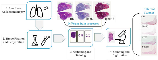
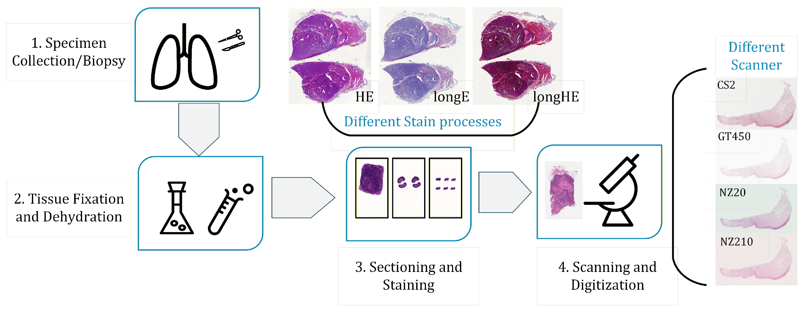
A typical WSI acquisition pipeline includes tissue fixation, paraffin embedding, sectioning, staining, and slide scanning. Figure 1 summarizes this workflow [2].

Figure 1. Typical workflow of WSIs imaging, illustrating color variations arising from staining and scanner differences. Staining protocol: standard H&E (HE), long time stained Eosin (longE), and long time stained H&E (longHE). Scanners: Aperio ScanScope CS2 (CS2), NanoZoomer 2.0-HT (NZ20), NanoZoomer S210 (NZ210), and Aperio GT 450 (GT450).

Clinically and technically, color variability can be introduced at multiple stages of this pipeline. Differences in tissue thickness, fixation time, reagent concentration, pH, staining duration, scanner optics, illumination, sensor response, and compression settings can all alter the final appearance of the digitized slide. Even when the underlying tissue morphology is similar, these factors can produce substantial changes in hue, saturation, contrast, and background tone.

Such variability creates practical difficulties for both human readers and algorithms. For pathologists, inconsistent staining complicates side-by-side comparison across hospitals, scanners, and archival time points. For computational pipelines, stain shift acts as a domain shift that can degrade detection, segmentation, and classification performance, especially when a model is deployed outside the institution where it was developed. In the whole-slide setting, the challenge is further amplified by the gigapixel scale of WSIs since normalization must remain stable under tiling and reassembly.

Therefore, a clinically useful stain normalization method should satisfy three requirements simultaneously: it should align chromatic statistics with a target style, preserve diagnostically relevant morphology, and scale to gigapixel WSIs without introducing tile-boundary artifacts. These requirements motivate the variational framework proposed in this paper.

1.2. Related Works

Stain normalization in digital pathology began with global color-transfer methods. Reinhard et al. [3] introduced mean–variance matching in the decorrelated Lab space, and subsequent variants refined the transformation through alternative color coordinates and matching criteria, including HSV/Lab projections [4,5,6], fuzzy-logic constraints [7,8], and optimal-transport formulations [9]. The appeal of this line of work lies in its simplicity and efficiency; however, because the transformation is prescribed globally, it may suppress local tissue microstructure when stain variation is spatially heterogeneous.

A second line of work moved from global color transfer to stain decomposition and morphology-aware normalization. Macenko et al. [10] estimated stain vectors in optical-density space via singular value decomposition, while Vahadane et al. [11] used sparse non-negative factorization to separate stain basis and concentration maps. Related approaches based on adaptive deconvolution [12], IDA decomposition [13], and geometry-aware alignment such as GCTI [14] further improved local structure preservation by explicitly exploiting stain geometry and local statistics. Their main limitation is not the lack of modeling, but rather the numerical sensitivity of stain-vector estimation and local statistics in low-variance, background-dominated, or strongly heterogeneous regions.

Meanwhile, the development of computational pathology has brought stain normalization increasingly into the scope of data-driven learning [15]. One line of work learns an explicit normalization map from curated data. StainNet [16] emphasizes a lightweight feed-forward architecture with fast inference, U-Net-based correction has also been investigated [17], and normalization-aware augmentation strategies have been proposed to improve robustness to stain variation [18]. Such models can be efficient once trained, but the cost of assembling representative data remains substantial in pathology, and the learned map may degrade when the staining or scanner distribution departs from the training domain.

Another line of work uses adversarial or generative transfer to relax the requirement of exact source–target pairing. Cycle-consistent normalization [19], StainGAN [20], adversarial stain transfer [21,22,23], style-transfer-based schemes [24,25], structure-preserved generation [26,27], SA-GAN [28], region-aware adversarial normalization [29], and recent multi-domain frameworks [30] can represent highly non-linear appearance changes that lie beyond affine or decomposition-based models. Their main difficulty is reliability: under domain mismatch, the generated image may contain hallucinated textures, checkerboard patterns, or style bias. In pathology [31,32], such artifacts are especially problematic because a visually plausible output is not sufficient unless diagnostically relevant morphology is also preserved.

From a mathematical viewpoint, these developments suggest a persistent trade-off. Classical statistical methods are explicit and efficient but weak in local structural control; stain-decomposition methods are more morphology-aware but can become unstable in degenerate regions; learning-based methods are more expressive but their robustness and transferability remain largely empirical. Building on these studies, we adopt a different route: starting from a reaction–diffusion interpretation of stain formation, we formulate normalization as a screened Poisson variational problem so that structural preservation, chromatic consistency, and whole-slide computability can be studied within a single framework.

1.3. Main Contributions

The main contributions of this paper are summarized as follows:

• We reformulate stain normalization as a variational inverse problem motivated by a reaction–diffusion interpretation of histological staining, and derive a screened Poisson (modified Helmholtz) model in the CIE $L^{*}{a}^{*}{b}^{*}$ space.
• We establish the analytical properties of the model in $H^1\left(\mathsf{\Omega }\right)$, including existence, uniqueness, and Lipschitz stability of the weak solution, thereby converting an ill-posed color-normalization task into a well-posed reconstruction problem.
• We prove an exponential localization property induced by the screening parameter, which yields a characteristic length scale ${𝓁}_c\sim {\lambda }^{-1/2}$ and provides a rigorous justification for non-overlapping domain decomposition on gigapixel WSIs.
• We develop a DCT-based tiled solver and validate it on multi-center datasets and a synthetic benchmark, showing that the proposed method achieves coherent whole-slide normalization while preserving diagnostically relevant morphology.

The remainder of this paper is organized as follows. Section 2 formulates stain normalization as an inverse problem and establishes its mathematical foundations. Section 3 derives the Screened Poisson Normalization (SPN) model from a reaction–diffusion interpretation in the CIE $L^{*}{a}^{*}{b}^{*}$ space. Section 4 proves well-posedness, Lipschitz stability, and exponential localization. Section 5 presents the finite-difference discretization, the DCT-based spectral solver, and the tiled implementation. Section 6 reports experimental results on multi-center datasets. Finally, Section 7 summarizes the main findings and discusses limitations and future work.

2. Mathematical Foundations

We define stain normalization as an inverse problem on a bounded Lipschitz domain $\mathsf{\Omega }\subset {\mathbb{R}}^2$. Let $I_S,I_T:\mathsf{\Omega }\to {\mathbb{R}}^3$ denote the source and reference images, respectively. The task is to recover a normalized field $u:\mathsf{\Omega }\to \mathbb{R}$ (processed channel-wise in the decorrelated CIE $Lab$ space [3]) that simultaneously satisfies structural fidelity to $I_S$ and statistical alignment with $I_T$. This section analyzes the ill-posed nature of this reconstruction and establishes its theoretical connection to reaction–diffusion physics.

2.1. Variational Formulation of the Inverse Problem

Mathematically, recovering u is fundamentally under-determined. The statistical constraint operator $\mathcal{C}\left(u\right)\approx \mathcal{C}\left(I_T\right)$ is non-injective, as infinite spatial configurations can share identical global moments. Conversely, relying solely on gradient fidelity $\nabla u\approx \nabla I_S$ determines the solution only up to an additive constant (the null space of the Neumann operator). Consequently, the unconstrained optimization is ill-posed in the sense of Hadamard [33]. To restore well-posedness, the problem must be cast within a Tikhonov regularization framework [34]. We seek a solution $u\in H^1\left(\mathsf{\Omega }\right)$ that minimizes a strictly convex energy functional of the form:

$$\mathcal{J}\left(u\right):={\displaystyle \frac{1}{2}}{\parallel \nabla u-\mathbf{g}\parallel }_{L^2\left(\mathsf{\Omega }\right)}^2+{\displaystyle \frac{\lambda }{2}}{\parallel u-T\parallel }_{L^2\left(\mathsf{\Omega }\right)}^2,\lambda >0.$$

(1)

Here, the first term enforces structural consistency with a guidance field $\mathbf{g}$ derived from the source, while the second term anchors the solution to a chromatic prior T. The regularization parameter $\lambda$ balances these competing objectives and ensures the coercivity of the bilinear form, guaranteeing the existence of a unique, stable weak solution.

2.2. Reaction–Diffusion Interpretation

The variational structure of (1) is not merely a mathematical regularization; it is motivated by the physical transport laws [35] governing histological staining. The accumulation of dye within porous tissue follows reaction–diffusion kinetics [36,37,38]. For a dye species with concentration $C(\mathbf{x},t)$, the governing equation is:

$${𝜕}_{t}C=\nabla ·(D\nabla C)+R(C,\mathbf{x}),$$

(2)

where D is the diffusion coefficient and R describes the binding reaction. Near chemical equilibrium, the binding process approximates linear kinetics $R\left(C\right)\approx -k(C-C_{\mathrm{eq}})$, where k is the reaction rate and $C_{\mathrm{eq}}$ is the local equilibrium concentration determined by tissue affinity.

At the thermodynamic steady state (${𝜕}_{t}C=0$), assuming isotropic diffusion, (2) reduces to the screened Poisson equation:

$$-\Delta C+\kappa C=\kappa C_{\mathrm{eq}},\mathrm{with}\kappa :=k/D.$$

(3)

This physical equilibrium (3) shares the exact Euler–Lagrange form of the variational problem (1). The regularization parameter $\lambda$ thus corresponds to the physical ratio of reaction to diffusion rates ($\kappa$), while the anchor T corresponds to the chemical equilibrium potential. This theoretical equivalence provides the physical basis for modeling stain normalization as a screened Poisson process. In practice, the chemical concentration field is not observed directly. Under the Beer–Lambert law, however, dye amount is linked to optical absorbance/optical density (OD), which is the standard physical intermediate used in histopathology color analysis; this provides the natural bridge from the reaction–diffusion description above to the digital image-domain formulation used in Section 3 [10,35,39].

3. The Screened Poisson Normalization (SPN) Model

This section details the Screened Poisson Normalization (SPN) model. Although the reaction–diffusion interpretation in Section 2 is expressed in terms of dye concentration, the observed pathology data arise through optical imaging; in histopathology, optical density (OD), motivated by the Beer–Lambert law, is the standard intermediate linking stain amount to image formation and thus provides the natural bridge to the image-domain variational formulation used here [10,35,39]. Accordingly, SPN is formulated directly in the perceptually decorrelated CIE $L^{*}{a}^{*}{b}^{*}$ space and solved channel-wise.

For each channel $c\in \{L^{*},a^{*},b^{*}\}$, we define the normalized field $u_c\in H^1\left(\mathsf{\Omega }\right)$ as the unique minimizer of the strictly convex energy functional:

$${\mathcal{J}}_c\left(u_c\right):={\int }_{\mathsf{\Omega }}\left({\displaystyle \frac{1}{2}}{\parallel \nabla u_c-{\mathbf{g}}_c\parallel }^2+{\displaystyle \frac{{\lambda }_c}{2}}{(u_c-T_c)}^2\right)d\mathbf{x}.$$

(4)

The first term ensures structural fidelity by penalizing gradient deviations from a guidance field ${\mathbf{g}}_c$, while the second acts as a Tikhonov regularizer, anchoring the solution to a chromatic prior $T_c$. The parameter ${\lambda }_c>0$ governs the trade-off between these objectives and ensures the problem is well-posed.

Minimizing (4) yields the associated Euler–Lagrange equation, which takes the form of a steady-state screened Poisson equation:

$$-\Delta u_c+{\lambda }_c{u}_c={\lambda }_c{T}_c-\nabla ·{\mathbf{g}}_c\mathrm{in}\mathsf{\Omega },$$

(5)

subject to the adiabatic boundary condition $(\nabla u_c-{\mathbf{g}}_c)·\mathbf{n}=0$ on $𝜕\mathsf{\Omega }$. Physically, this equation describes a diffusion process driven by a source term $f_c:={\lambda }_c{T}_c-\nabla ·{\mathbf{g}}_c$, which balances the injection of high-frequency morphological details with low-frequency chromatic information.

Remark 1

(Boundary-condition choice). The boundary condition in (5),

$$(\nabla u_c-{\mathbf{g}}_c)·\mathbf{n}=0\mathrm{on}𝜕\mathsf{\Omega },$$

is the natural Euler–Lagrange condition of the variational functional (4). In the present work this choice is also computationally advantageous: on rectangular image domains it is compatible with the cosine basis used by the DCT solver in Section 5.2. Prescribed Dirichlet data on rectangular domains can still be treated spectrally after boundary lifting, typically with a sine-transform basis. Mixed boundary conditions or irregular tile geometries, however, generally lose the simple separable diagonalization and are more naturally handled by iterative solvers. Since tile boundaries in gigapixel processing are artificial rather than physically observed, the natural Neumann closure is the most appropriate default for the non-overlapping tiled implementation studied here. In the tiled WSI setting, the most relevant boundaries are the artificial tile interfaces rather than physically observed object boundaries; for these computational interfaces, the natural Neumann closure is the most appropriate default.

To close the system, we construct the chromatic anchor $T_c$ and guidance field ${\mathbf{g}}_c$ from the source $I_S$ and reference $I_T$. The anchor $T_c$ is defined by matching the global mean $\mu$ and standard deviation $\sigma$ of the reference:

$$T_c\left(\mathbf{x}\right)={\displaystyle \frac{{\sigma }_T^{\left(c\right)}}{{\sigma }_S^{\left(c\right)}}}\left({\left(I_S\right)}_c\left(\mathbf{x}\right)-{\mu }_S^{\left(c\right)}\right)+{\mu }_T^{\left(c\right)}.$$

(6)

This linear mapping provides a stable baseline for chromaticity that is robust to local variations. To preserve morphology, we parameterize the guidance field ${\mathbf{g}}_c$ as a spatially varying blend of source and anchor gradients:

$${\mathbf{g}}_c\left(\mathbf{x}\right)=(1-w\left(\mathbf{x}\right)){\alpha }_c\nabla {\left(I_S\right)}_c\left(\mathbf{x}\right)+w\left(\mathbf{x}\right)\nabla T_c\left(\mathbf{x}\right),$$

(7)

where ${\alpha }_c$ is a robust contrast factor defined by the ratio of median gradient magnitudes, i.e., ${\alpha }_c=median\parallel \nabla {\left(I_T\right)}_c\parallel /median\parallel \nabla {\left(I_S\right)}_c\parallel$. The structural weight $w\left(\mathbf{x}\right)\in (0,1]$ is derived from the source luminance channel $I_{S,L^{*}}$ via:

$$w\left(\mathbf{x}\right)=exp\left(-{\displaystyle \frac{\parallel \nabla I_{S,L^{*}}{\left(\mathbf{x}\right)\parallel }^2}{{\tau }^2}}\right),\tau >0.$$

(8)

In structurally salient regions ($w\to 0$), the guidance field strictly adheres to the source morphology $\nabla {\left(I_S\right)}_c$, whereas in homogeneous regions, the model relaxes toward the smooth chromatic anchor. The resulting solution corresponds to the steady state of a system with screening length ${𝓁}_c\sim {\lambda }_c^{-1/2}$, preventing local artifacts from propagating globally.

4. Theoretical Analysis

This section analyzes the mathematical properties of the Screened Poisson Normalization (SPN) model. Since the SPN system is solved channel-wise, we fix a channel $c\in \{L^{*},a^{*},b^{*}\}$ throughout this section and keep the subscript c explicitly in order to maintain notational consistency with Section 3. Thus $u_c\in H^1\left(\mathsf{\Omega }\right)$ denotes the weak solution of (5), $I_{S,c}:={\left(I_S\right)}_c$, $T_c$ is the chromatic anchor, ${\mathbf{g}}_c$ is the guidance field, and ${\lambda }_c>0$ is the corresponding screening parameter.

The variational problem derived in Section 3 is equivalent to finding a weak solution $u_c\in H^1\left(\mathsf{\Omega }\right)$ such that

$$B_c(u_c,v)=F_c\left(v\right),\forall v\in H^1\left(\mathsf{\Omega }\right),$$

(9)

where the bilinear form $B_c:H^1\left(\mathsf{\Omega }\right)\times H^1\left(\mathsf{\Omega }\right)\to \mathbb{R}$ and the linear functional $F_c:H^1\left(\mathsf{\Omega }\right)\to \mathbb{R}$ are defined by

$$B_c(u_c,v):={\int }_{\mathsf{\Omega }}\left(\nabla u_c·\nabla v+{\lambda }_c{u}_{c}v\right)d\mathbf{x},F_c\left(v\right):={\int }_{\mathsf{\Omega }}\left({\mathbf{g}}_c·\nabla v+{\lambda }_c{T}_{c}v\right)d\mathbf{x}.$$

We assume $\mathsf{\Omega }\subset {\mathbb{R}}^2$ is a bounded Lipschitz domain, ${\lambda }_c>0$, ${\mathbf{g}}_c\in {\left[L^2\left(\mathsf{\Omega }\right)\right]}^2$, and $T_c\in L^2\left(\mathsf{\Omega }\right)$.

Theorem 1

(Existence and uniqueness). For any fixed channel c, screening parameter ${\lambda }_c>0$, guidance field ${\mathbf{g}}_c\in {\left[L^2\left(\mathsf{\Omega }\right)\right]}^2$, and chromatic anchor $T_c\in L^2\left(\mathsf{\Omega }\right)$, the variational problem (9) admits a unique solution $u_c^{*}\in H^1\left(\mathsf{\Omega }\right)$.

Proof. 

The result follows from the Lax–Milgram theorem. First, the bilinear form $B_c$ is continuous on $H^1\left(\mathsf{\Omega }\right)\times H^1\left(\mathsf{\Omega }\right)$:

$$|B_c(u_c,v)| \le \parallel \nabla u_c{\parallel }_{L^2}{\parallel \nabla v\parallel }_{L^2}+{\lambda }_c\parallel u_c{\parallel }_{L^2}{\parallel v\parallel }_{L^2}\le max(1,{\lambda }_c)\parallel u_c{\parallel }_{H^1}{\parallel v\parallel }_{H^1}.$$

Second, $B_c$ is coercive:

$$B_c(u_c,u_c)= \parallel \nabla u_c{\parallel }_{L^2}^2+{\lambda }_c\parallel u_c{\parallel }_{L^2}^2 \ge min(1,{\lambda }_c){\parallel u_c\parallel }_{H^1}^2.$$

Finally,

$$|F_c\left(v\right)|\le \parallel {\mathbf{g}}_c{\parallel }_{L^2}{\parallel \nabla v\parallel }_{L^2}+{\lambda }_c\parallel T_c{\parallel }_{L^2}{\parallel v\parallel }_{L^2}\le \left(\parallel {\mathbf{g}}_c{\parallel }_{L^2}+ {\lambda }_c{\parallel T_c\parallel }_{L^2}\right){\parallel v\parallel }_{H^1},$$

so $F_c$ is bounded on $H^1\left(\mathsf{\Omega }\right)$. The theorem follows.    □

With the channel-wise solution uniquely defined, we quantify its stability with respect to perturbations in the input data $({\mathbf{g}}_c,T_c)$.

Theorem 2

(Lipschitz stability). Let $u_{1,c},u_{2,c}\in H^1\left(\mathsf{\Omega }\right)$ be the unique weak solutions corresponding to data $({\mathbf{g}}_{1,c},T_{1,c})$ and $({\mathbf{g}}_{2,c},T_{2,c})$, respectively. Then

$${\parallel u_{1,c}-u_{2,c}\parallel }_{H^1\left(\mathsf{\Omega }\right)} \le {\displaystyle \frac{1}{min(1,{\lambda }_c)}}\left(\parallel {\mathbf{g}}_{1,c}-{\mathbf{g}}_{2,c}{\parallel }_{L^2\left(\mathsf{\Omega }\right)}+ {\lambda }_c{\parallel T_{1,c}-T_{2,c}\parallel }_{L^2\left(\mathsf{\Omega }\right)}\right).$$

(10)

Proof. 

Let $w_c:=u_{1,c}-u_{2,c}$. Subtracting the two weak formulations gives

$$B_c(w_c,v)={\int }_{\mathsf{\Omega }}\left(({\mathbf{g}}_{1,c}-{\mathbf{g}}_{2,c})·\nabla v+{\lambda }_c(T_{1,c}-T_{2,c})v\right)d\mathbf{x},\forall v\in H^1\left(\mathsf{\Omega }\right).$$

Choosing $v=w_c$ and using coercivity and Cauchy–Schwarz,

$$min(1,{\lambda }_c){\parallel w_c\parallel }_{H^1}^2\le B_c(w_c,w_c)\le \left({\parallel {\mathbf{g}}_{1,c}-{\mathbf{g}}_{2,c}\parallel }_{L^2}+ {\lambda }_c{\parallel T_{1,c}-T_{2,c}\parallel }_{L^2}\right){\parallel w_c\parallel }_{H^1}.$$

Dividing by $\parallel w_c{\parallel }_{H^1}$ gives (10).    □

The preceding $H^1$ theory is sufficient for well-posedness. For the rectangular domains used in the numerical section, one can further recover $H^2$ regularity under mild additional smoothness assumptions on the data.

Proposition 1

(Elliptic regularity on rectangular domains). Let $\mathsf{\Omega }=(0,L_x)\times (0,L_y)$ and let ${\lambda }_c>0$. Assume $T_c\in H^1\left(\mathsf{\Omega }\right)$ and ${\mathbf{g}}_c\in {\left[H^1\left(\mathsf{\Omega }\right)\right]}^2$. Then the unique weak solution $u_c\in H^1\left(\mathsf{\Omega }\right)$ of (5) belongs to $H^2\left(\mathsf{\Omega }\right)$ and satisfies

$${\parallel u_c\parallel }_{H^2\left(\mathsf{\Omega }\right)}\le C_{\mathsf{\Omega },{\lambda }_c}\left({\lambda }_c{\parallel T_c\parallel }_{L^2\left(\mathsf{\Omega }\right)}+ \parallel \nabla ·{\mathbf{g}}_c{\parallel }_{L^2\left(\mathsf{\Omega }\right)}+{\parallel {\mathbf{g}}_c·\mathbf{n}\parallel }_{H^{1/2}(𝜕\mathsf{\Omega })}\right).$$

(11)

Proof. 

Since ${\mathbf{g}}_c\in {\left[H^1\left(\mathsf{\Omega }\right)\right]}^2$, we have

$$f_c:={\lambda }_c{T}_c-\nabla ·{\mathbf{g}}_c\in L^2\left(\mathsf{\Omega }\right),h_c:={\mathbf{g}}_c·\mathbf{n}\in H^{1/2}(𝜕\mathsf{\Omega }).$$

Equation (5) can therefore be rewritten as

$$-\Delta u_c+{\lambda }_c{u}_c=f_c\mathrm{in}\mathsf{\Omega },{𝜕}_n{u}_c=h_c\mathrm{on}𝜕\mathsf{\Omega }.$$

Because ${\lambda }_c>0$, no compatibility condition is required. Standard elliptic regularity for the Neumann problem on rectangles yields $u_c\in H^2\left(\mathsf{\Omega }\right)$ and (11).    □

Remark 2.

The bounded Lipschitz assumption used in Theorem 1 is sufficient for existence and uniqueness. The stronger rectangular-domain assumption in Proposition 1 is introduced only to connect the continuous analysis with the rectangular-tile discretization and DCT solver used in Section 5.

Lemma 1

(Energy comparison principle). Let $u_c^{*}$ be the global minimizer of ${\mathcal{J}}_c$. For any comparison function $v_c\in H^1\left(\mathsf{\Omega }\right)$,

$${\parallel \nabla u_c^{*}-{\mathbf{g}}_c\parallel }_{L^2\left(\mathsf{\Omega }\right)}^2+ {\lambda }_c{\parallel u_c^{*}-T_c\parallel }_{L^2\left(\mathsf{\Omega }\right)}^2 \le {\parallel \nabla v_c-{\mathbf{g}}_c\parallel }_{L^2\left(\mathsf{\Omega }\right)}^2+ {\lambda }_c{\parallel v_c-T_c\parallel }_{L^2\left(\mathsf{\Omega }\right)}^2.$$

(12)

Proof. 

This is an immediate consequence of the optimality condition

$${\mathcal{J}}_c\left(u_c^{*}\right)\le {\mathcal{J}}_c\left(v_c\right).$$

   □

Theorem 3

(Guidance fidelity bound). Let $u_c^{*}$ be the minimizer of ${\mathcal{J}}_c$. Then

$$\parallel \nabla u_c^{*}-{\mathbf{g}}_c{\parallel }_{L^2\left(\mathsf{\Omega }\right)} \le \parallel \nabla I_{S,c}-{\mathbf{g}}_c{\parallel }_{L^2\left(\mathsf{\Omega }\right)}+ \sqrt{{\lambda }_c}{\parallel I_{S,c}-T_c\parallel }_{L^2\left(\mathsf{\Omega }\right)}.$$

(13)

Proof. 

Set $v_c=I_{S,c}$ in Lemma 1. Then

$$\parallel \nabla u_c^{*}-{\mathbf{g}}_c{\parallel }_{L^2\left(\mathsf{\Omega }\right)}^2 \le \parallel \nabla I_{S,c}-{\mathbf{g}}_c{\parallel }_{L^2\left(\mathsf{\Omega }\right)}^2+ {\lambda }_c{\parallel I_{S,c}-T_c\parallel }_{L^2\left(\mathsf{\Omega }\right)}^2.$$

Taking square roots and using $\sqrt{a^2+b^2}\le a+b$ yields (13).    □

Corollary 1

(Deviation from the source morphology). The normalized gradient field remains close to the source gradient in the sense that

$${\parallel \nabla u_c^{*}-\nabla I_{S,c}\parallel }_{L^2\left(\mathsf{\Omega }\right)} \le 2{\parallel \nabla I_{S,c}-{\mathbf{g}}_c\parallel }_{L^2\left(\mathsf{\Omega }\right)} + \sqrt{{\lambda }_c}{\parallel I_{S,c}-T_c\parallel }_{L^2\left(\mathsf{\Omega }\right)}.$$

(14)

Proof. 

By the triangle inequality,

$$\parallel \nabla u_c^{*}-\nabla I_{S,c}{\parallel }_{L^2} \le \parallel \nabla u_c^{*}-{\mathbf{g}}_c{\parallel }_{L^2}+{\parallel {\mathbf{g}}_c-\nabla I_{S,c}\parallel }_{L^2}.$$

Applying Theorem 3 gives (14).    □

We now quantify the localization of tile-interface errors on the rectangular tiles used in the implementation. Let

$${\mathsf{\Omega }}_k=(0,a_k)\times (0,b_k),{\Gamma }_k:=𝜕{\mathsf{\Omega }}_k\setminus 𝜕\mathsf{\Omega },$$

and let $u_c$ be the global solution of (5). $u_{c,k}$ denotes the local tile solution obtained by solving the same interior equation on ${\mathsf{\Omega }}_k$ with the tile-wise Neumann closure used by the algorithm. The error

$$e_{c,k}:=u_c{|}_{{\mathsf{\Omega }}_k}-u_{c,k}$$

then solves

$$\left\{\begin{array}{cc}-\Delta e_{c,k}+{\lambda }_c{e}_{c,k}=0,\hfill & \mathrm{in}{\mathsf{\Omega }}_k,\hfill \\ {𝜕}_n{e}_{c,k}=0,\hfill & \mathrm{on}𝜕{\mathsf{\Omega }}_k\cap 𝜕\mathsf{\Omega },\hfill \\ {𝜕}_n{e}_{c,k}={\psi }_{c,k},\hfill & \mathrm{on}{\Gamma }_k,\hfill \end{array}\right.$$

(15)

where

$${\psi }_{c,k}:=(\nabla u_c-{\mathbf{g}}_c)·\mathbf{n}\mathrm{on}{\Gamma }_k.$$

Lemma 2

(Rectangular Neumann Green function). Let $N_{k,{\lambda }_c}(\mathbf{x},\mathbf{y})$ be the Green function of $-\Delta +{\lambda }_c$ on ${\mathsf{\Omega }}_k=(0,a_k)\times (0,b_k)$ with homogeneous Neumann boundary condition. Then

$$N_{k,{\lambda }_c}(\mathbf{x},\mathbf{y})=\sum _{m,n\ge 0}{\displaystyle \frac{{\varphi }_{mn}^{\left(k\right)}\left(\mathbf{x}\right){\varphi }_{mn}^{\left(k\right)}\left(\mathbf{y}\right)}{{\lambda }_c+{\mu }_{mn}^{\left(k\right)}}},$$

(16)

where

$${\mu }_{mn}^{\left(k\right)}={\left({\displaystyle \frac{m\pi }{a_k}}\right)}^2+{\left({\displaystyle \frac{n\pi }{b_k}}\right)}^2,{\varphi }_{mn}^{\left(k\right)}(x_1,x_2)={\beta }_m^{\left(a_k\right)}{\beta }_n^{\left(b_k\right)}cos\left({\displaystyle \frac{m\pi x_1}{a_k}}\right)cos\left({\displaystyle \frac{n\pi x_2}{b_k}}\right),$$

with

$${\beta }_0^{\left(a\right)}=a^{-1/2},{\beta }_m^{\left(a\right)}=\sqrt{2/a}(m\ge 1).$$

Moreover, if

$${\eta }_k:={\displaystyle \frac{max\{a_k,b_k\}}{min\{a_k,b_k\}}},$$

then there exists a constant $C_{{\eta }_k}>0$, depending only on the aspect ratio ${\eta }_k$, such that

$$|N_{k,{\lambda }_c}(\mathbf{x},\mathbf{y})|\le C_{{\eta }_k}{\lambda }_c^{-1/4}{|\mathbf{x}-\mathbf{y}|}^{-1/2}{e}^{-\sqrt{{\lambda }_c}|\mathbf{x}-\mathbf{y}|}\mathit{for}\mathit{all}\mathbf{x}\ne \mathbf{y}\mathit{in}{\mathsf{\Omega }}_k.$$

(17)

Proof. 

The representation (16) is the standard cosine-eigenfunction expansion of the Neumann Green function on a rectangle; see, e.g., [40,41]. The pointwise estimate (17) is a standard modified-Helmholtz Green-function bound on shape-regular rectangles. Indeed, the reflected cosine series can be compared with the free-space kernel

$$G_{{\lambda }_c}\left(r\right)={\displaystyle \frac{1}{2\pi }}{K}_0\left(\sqrt{{\lambda }_c}r\right),$$

and the large-argument asymptotics of the modified Bessel function $K_0$ yield

$$K_0\left(s\right)=\sqrt{{\displaystyle \frac{\pi }{2s}}}{e}^{-s}\left(1+O\left(s^{-1}\right)\right)(s\to \infty ),$$

while the local singularity remains only logarithmic as $s\downarrow 0$, and is therefore dominated by $s^{-1/2}$. Hence

$$|G_{{\lambda }_c}\left(r\right)|\le C{\lambda }_c^{-1/4}{r}^{-1/2}{e}^{-\sqrt{{\lambda }_c}r},r>0.$$

The same bound carries over to the rectangular Neumann Green function, up to a constant depending only on the aspect ratio ${\eta }_k$, because the reflected image/cosine series is uniformly controlled on shape-regular rectangles; see [41].    □

Theorem 4

(Exponential localization of interface error on rectangular tiles). Let $e_{c,k}$ solve (15). Then, for every $\mathbf{x}\in {\mathsf{\Omega }}_k$ with $d(\mathbf{x},{\Gamma }_k)>0$,

$$\left|e_{c,k}\right(\mathbf{x}\left)\right|\le C_{{\eta }_k}|{\Gamma }_k{|}^{1/2}{\lambda }_c^{-1/4}d{(\mathbf{x},{\Gamma }_k)}^{-1/2}exp\left(-\sqrt{{\lambda }_c}d(\mathbf{x},{\Gamma }_k)\right){\parallel {\psi }_{c,k}\parallel }_{L^2\left({\Gamma }_k\right)}.$$

(18)

In particular, if all tiles are congruent with side lengths $a\times b$, then $|{\Gamma }_k| \le 2(a+b)$ and the constant in (18) is uniform over all tiles, depending only on the fixed aspect ratio

$$\eta ={\displaystyle \frac{max\{a,b\}}{min\{a,b\}}}.$$

Proof. 

By Green’s representation for (15),

$$e_{c,k}\left(\mathbf{x}\right)={\int }_{{\Gamma }_k}{N}_{k,{\lambda }_c}(\mathbf{x},\mathbf{y}){\psi }_{c,k}\left(\mathbf{y}\right)d\sigma \left(\mathbf{y}\right).$$

Applying Cauchy–Schwarz,

$$\left|e_{c,k}\right(\mathbf{x}\left)\right|\le \parallel N_{k,{\lambda }_c}{(\mathbf{x},·)\parallel }_{L^2\left({\Gamma }_k\right)}{\parallel {\psi }_{c,k}\parallel }_{L^2\left({\Gamma }_k\right)}.$$

For $\mathbf{y}\in {\Gamma }_k$, one has

$$|\mathbf{x}-\mathbf{y}|\ge d(\mathbf{x},{\Gamma }_k).$$

Since the function $r\mapsto r^{-1/2}{e}^{-\sqrt{{\lambda }_c}r}$ is decreasing for $r>0$, Lemma 2 gives

$$|N_{k,{\lambda }_c}(\mathbf{x},\mathbf{y})|\le C_{{\eta }_k}{\lambda }_c^{-1/4}d{(\mathbf{x},{\Gamma }_k)}^{-1/2}{e}^{-\sqrt{{\lambda }_c}d(\mathbf{x},{\Gamma }_k)}.$$

Therefore,

$${\parallel N_{k,{\lambda }_c}(\mathbf{x},·)\parallel }_{L^2\left({\Gamma }_k\right)}\le C_{{\eta }_k}{\left|{\Gamma }_k\right|}^{1/2}{\lambda }_c^{-1/4}d{(\mathbf{x},{\Gamma }_k)}^{-1/2}{e}^{-\sqrt{{\lambda }_c}d(\mathbf{x},{\Gamma }_k)},$$

which proves (18).    □

Remark 3.

Equation (18) makes the geometric dependence explicit: for a fixed rectangular tiling, the prefactor is controlled by the interface length $|{\Gamma }_k|$ and the tile aspect ratio. The dominant decay scale remains the screening length

$${𝓁}_c={\lambda }_c^{-1/2},$$

while the algebraic factor $d{(\mathbf{x},{\Gamma }_k)}^{-1/2}$ is the standard two-dimensional Green-function prefactor. In practice, once the interior point lies a few screening lengths away from the interface, the exponential factor dominates.

Remark 4.

Theorem 4 implies that tile-boundary perturbations are confined to a narrow interface layer. For sufficiently large tiles, the interior solution converges rapidly to the global reconstruction, which gives the analytical justification for non-overlapping domain decomposition in the screened setting considered here.

5. Optimization and Implementation

For each channel $c\in \{L^{*},a^{*},b^{*}\}$, the continuous SPN unknown is denoted by $u_c$, while its discrete approximation on a rectangular tile ${\mathsf{\Omega }}_k^h$ is denoted by $U_{c,k}\in {\mathbb{R}}^{H_k\times W_k}$.

5.1. Discrete SPN Equation on a Rectangular Tile

Each tile ${\mathsf{\Omega }}_k$ is a rectangle sampled on a Cartesian grid ${\mathsf{\Omega }}_k^h$ of size $H_k\times W_k$. In the actual implementation the pixel spacing is one, but we retain $h_x$ and $h_y$ below to make the consistency discussion explicit. We use $u_c$ for the continuous channel and $U_{c,k}$ for its discrete counterpart on tile ${\mathsf{\Omega }}_k^h$.

For a grid function $U\in {\mathbb{R}}^{H_k\times W_k}$, the discrete gradient is computed componentwise by centered differences in the interior and one-sided differences on the outermost grid layer:

$${\left(D_x^{h}U\right)}_{i,j}=\left\{\begin{array}{cc}(U_{i+1,j}-U_{i,j})/h_x,\hfill & i=0,\hfill \\ (U_{i+1,j}-U_{i-1,j})/\left(2h_x\right),\hfill & 1\le i\le H_k-2,\hfill \\ (U_{i,j}-U_{i-1,j})/h_x,\hfill & i=H_k-1,\hfill \end{array}\right.{\left(D_y^{h}U\right)}_{i,j}=\left\{\begin{array}{cc}(U_{i,j+1}-U_{i,j})/h_y,\hfill & j=0,\hfill \\ (U_{i,j+1}-U_{i,j-1})/\left(2h_y\right),\hfill & 1\le j\le W_k-2,\hfill \\ (U_{i,j}-U_{i,j-1})/h_y,\hfill & j=W_k-1.\hfill \end{array}\right.$$

(19)

We write ${\nabla }_{h}U:=(D_x^{h}U,D_y^{h}U)$, and for a vector field $\mathbf{q}=(q_x,q_y)$ we define

$${\nabla }_h·\mathbf{q}:=D_x^h{q}_x+D_y^h{q}_y.$$

(20)

This is the same centered/one-sided differentiation rule implemented by np.gradient in the code.

For the screened operator itself, we use the standard reflective five-point Laplacian,

$${\left({\Delta }_{h}U\right)}_{i,j}={\displaystyle \frac{U_{i^{+},j}-2U_{i,j}+U_{i^{-},j}}{h_x^2}}+{\displaystyle \frac{U_{i,j^{+}}-2U_{i,j}+U_{i,j^{-}}}{h_y^2}},$$

(21)

where $i^{-}:=max\{i-1,0\}$, $i^{+}:=min\{i+1,H_k-1\}$ and analogously for $j^{\pm }$. This is the rectangular Neumann stencil diagonalized by the DCT basis.

The tile-wise guidance field is assembled from a local patch $P_k:=I_S{|}_{{\mathsf{\Omega }}_k}$ and slide-level scalar priors. For each channel c,

$$T_{c,k}\left(\mathbf{x}\right)={\displaystyle \frac{{\sigma }_T^{\left(c\right)}}{{\sigma }_{S,\mathrm{glob}}^{\left(c\right)}}}\left({\left(P_k\right)}_c\left(\mathbf{x}\right)-{\mu }_{S,\mathrm{glob}}^{\left(c\right)}\right)+{\mu }_T^{\left(c\right)},$$

(22)

$${\alpha }_c={\displaystyle \frac{{med}_{{\mathsf{\Omega }}_h}\left|{\nabla }_h{\left(I_T\right)}_c\right|}{{med}_{{\mathsf{\Omega }}_h}\left|{\nabla }_h{\left(I_S\right)}_c\right|+\epsilon }},w_k\left(\mathbf{x}\right)=exp\left(-{\displaystyle \frac{|{\nabla }_h{\left(P_k\right)}_{L^{*}}\left(\mathbf{x}\right){|}^2}{{\tau }^2}}\right),$$

(23)

and

$${\mathbf{g}}_{c,k}=(1-w_k){\alpha }_c{\nabla }_h{\left(P_k\right)}_c+w_k{\nabla }_h{T}_{c,k}.$$

(24)

Here ${\mu }_{S,\mathrm{glob}}^{\left(c\right)}$, ${\sigma }_{S,\mathrm{glob}}^{\left(c\right)}$, ${\mu }_T^{\left(c\right)}$, ${\sigma }_T^{\left(c\right)}$, and ${\alpha }_c$ are computed once at the slide level and reused for every tile. Consequently, the chromatic prior is globally coherent, while only the pointwise weight $w_k$ and local gradients are tile dependent. Since $w_k$ is computed from the local patch, it differs from the restriction of a hypothetical global weight only within a one-grid-cell layer near the tile boundary; this produces a localized screened perturbation of the same interface-local character as that analyzed in Theorem 4.

The discrete tile equation solved in the implementation is

$$({\Delta }_h-{\lambda }_{c}I)U_{c,k}={\rho }_{c,k},{\rho }_{c,k}:={\nabla }_h·{\mathbf{g}}_{c,k}-{\lambda }_c{T}_{c,k}.$$

(25)

The sign convention in (25) matches the code and the DCT filter used in all experiments.

5.2. DCT Diagonalization on Rectangular Tiles

For a rectangular tile with reflective Neumann closure, the discrete Laplacian (21) is diagonalized by the 2D DCT-II basis. Let $\mathcal{F}$ denote the orthonormal forward DCT-II and ${\mathcal{F}}^{-1}$ its inverse DCT-III [40]. For $0\le u<H_k$ and $0\le v<W_k$, the eigenvalues of (21) are

$${\Lambda }_{u,v}^{\left(k\right)}={\displaystyle \frac{2}{h_x^2}}\left(cos{\displaystyle \frac{\pi u}{H_k}}-1\right)+{\displaystyle \frac{2}{h_y^2}}\left(cos{\displaystyle \frac{\pi v}{W_k}}-1\right),{\Lambda }_{u,v}^{\left(k\right)}\le 0.$$

(26)

Applying $\mathcal{F}$ to (25) decouples the system mode by mode:

$$({\Lambda }_{u,v}^{\left(k\right)}-{\lambda }_c){\widehat{U}}_{c,k}(u,v)={\widehat{\rho }}_{c,k}(u,v).$$

(27)

Thus

$${\widehat{U}}_{c,k}(u,v)={\displaystyle \frac{{\widehat{\rho }}_{c,k}(u,v)}{{\Lambda }_{u,v}^{\left(k\right)}-{\lambda }_c}},U_{c,k}={\mathcal{F}}^{-1}\left\{{\widehat{U}}_{c,k}\right\}.$$

(28)

When $h_x=h_y=1$, (26) reduces exactly to the formula used in the current implementation.

Discrete Meaning of the Natural Boundary Condition

The continuous condition $(\nabla u_c-{\mathbf{g}}_c)·\mathbf{n}=0$ is realized here in variational form: the screened operator is diagonalized with reflective Neumann closure, while the guidance field enters through the divergence-form forcing ${\nabla }_h·{\mathbf{g}}_{c,k}$. Hence the scheme does not impose ${𝜕}_n{u}_c=0$ independently of ${\mathbf{g}}_c$; rather, it is the discrete counterpart of the natural flux balance of (4).

Proposition 2 

(Discrete stability). For every tile ${\mathsf{\Omega }}_k^h$ and channel c, the operator ${\Delta }_h-{\lambda }_{c}I$ is invertible. Moreover,

$${\parallel U_{c,k}\parallel }_2\le {\lambda }_c^{-1}{\parallel {\rho }_{c,k}\parallel }_2,{\parallel U_{c,k}-V_{c,k}\parallel }_2 \le {\lambda }_c^{-1}{\parallel {\rho }_{c,k}-{\tilde{\rho }}_{c,k}\parallel }_2.$$

(29)

Proof. 

By (27), each spectral mode is divided by ${\Lambda }_{u,v}^{\left(k\right)}-{\lambda }_c$. Since ${\Lambda }_{u,v}^{\left(k\right)}\le 0$, one has

$$|{\Lambda }_{u,v}^{\left(k\right)}-{\lambda }_c| \ge {\lambda }_c.$$

Parseval’s identity then gives

$${\parallel U_{c,k}\parallel }_2^2=\sum _{u,v}{|{\widehat{U}}_{c,k}(u,v)|}^2\le {\lambda }_c^{-2}\sum _{u,v}{|{\widehat{\rho }}_{c,k}(u,v)|}^2={\lambda }_c^{-2}{\parallel {\rho }_{c,k}\parallel }_2^2.$$

The difference estimate follows identically by subtracting two right-hand sides.    □

Proposition 3 

(Abstract discretization error bound). Let $u_c$ be a smooth exact solution of (5) on a rectangular tile, let $I_h{u}_c$ denote its sampling on ${\mathsf{\Omega }}_k^h$, and let $U_{c,k}$ solve (25) with sampled data. Then

$${\parallel U_{c,k}-I_h{u}_c\parallel }_2 \le {\lambda }_c^{-1}\parallel ({\Delta }_h-{\lambda }_{c}I)I_h{u}_c-{\rho }_{c,k}{\parallel }_2.$$

(30)

Consequently, if the local truncation error of the chosen stencil is $O\left(h^p\right)$ for the sampled smooth data, then ${\parallel U_{c,k}-I_h{u}_c\parallel }_2 =O\left(h^p\right)$.

Proof. 

Subtract the discrete equation satisfied by $U_{c,k}$ from the residual of $I_h{u}_c$, and apply Proposition 2.    □

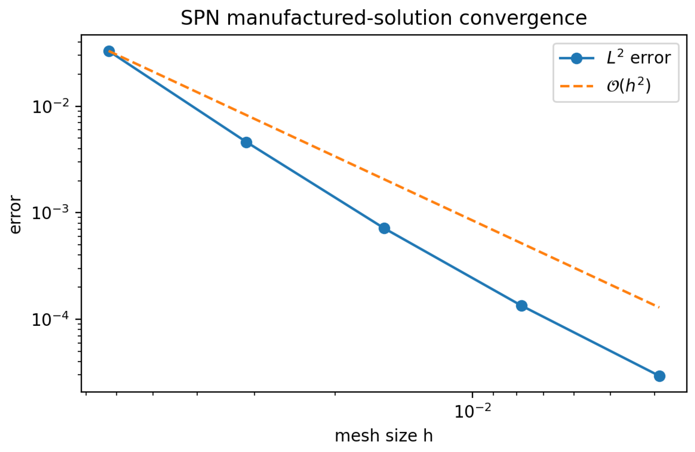
To complement the abstract stability/consistency statement in Proposition 3, Appendix A reports a manufactured-solution grid-refinement test for the same rectangular DCT solver and the same screened Poisson sign convention (25)–(28). The observed $L^2$ and $L^{\infty }$ errors decrease at an approximately second-order rate for smooth data, which confirms the practical convergence behavior of the discrete solver on rectangular grids.

5.3. Tiled SPN Implementation for Gigapixel WSIs

Direct application of the spectral solver to a full-resolution WSI is impractical due to memory constraints. We therefore adopt a non-overlapping domain decomposition [42] where the slide domain $\mathsf{\Omega }$ is partitioned into tiles ${\left\{{\mathsf{\Omega }}_k\right\}}_{k=1}^K$. The key requirement is that each local problem uses globally shared scalar priors, so that the tiled reconstruction remains consistent with the global SPN model up to localized interface effects.

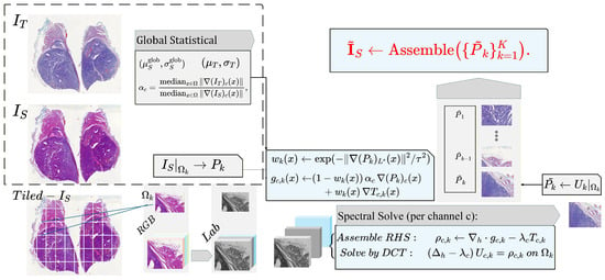
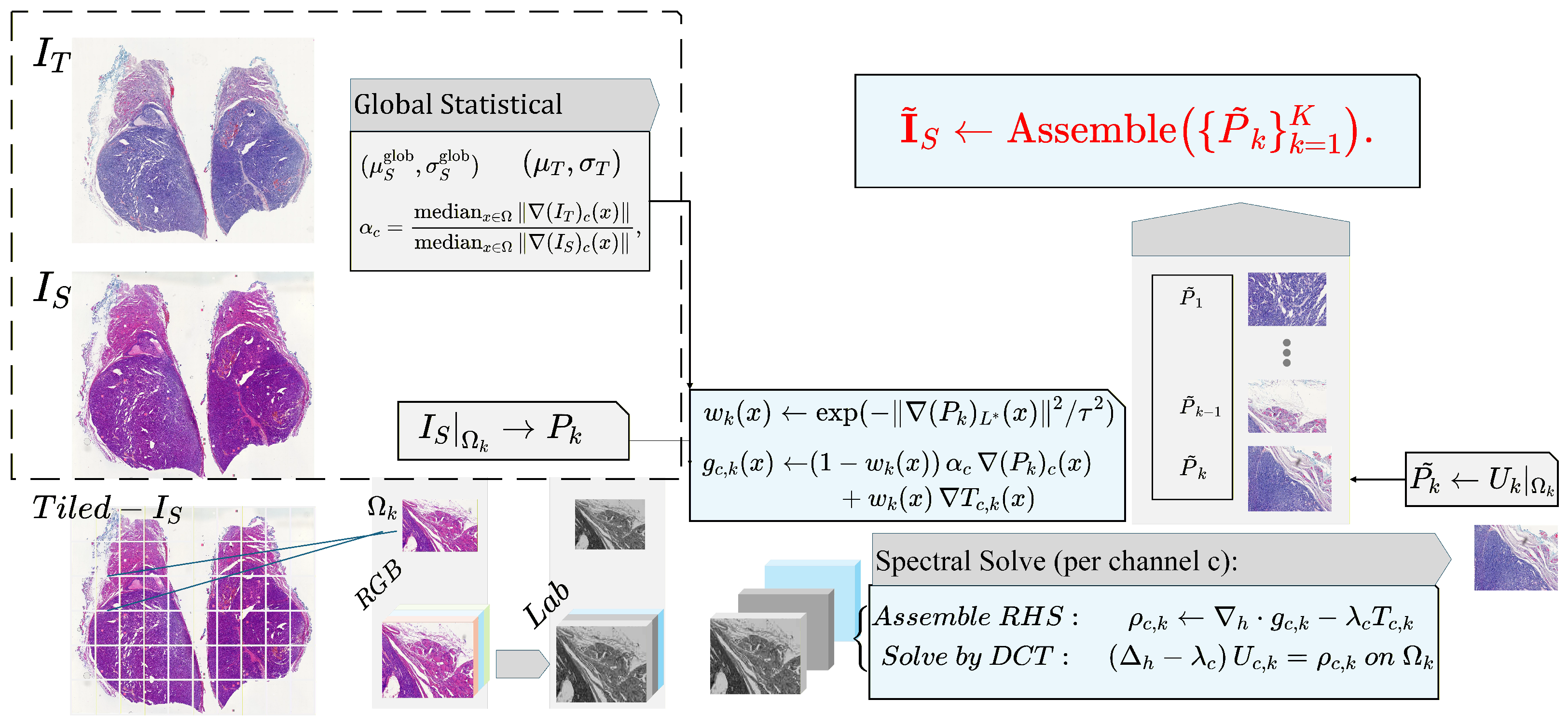
Our implementation consists of two phases. Before presenting the details, we summarize the tiled SPN implementation in Figure 2 and Algorithm 1.

Figure 2. Tiled SPN pipeline. In the first phase, we compute slide-level global prior statistics. In the second phase, we restrict these priors to each tile and solve the screened Poisson equation using a DCT-based spectral solver, assembling the normalized tiles into a coherent WSI.

Phase 1: slide-level scalar priors. For each channel c, we compute the global source moments $({\mu }_{S,\mathrm{glob}}^{\left(c\right)},{\sigma }_{S,\mathrm{glob}}^{\left(c\right)})$, the target moments $({\mu }_T^{\left(c\right)},{\sigma }_T^{\left(c\right)})$, and the global median gradient magnitudes

$$m_S^{\left(c\right)}={med}_{{\mathsf{\Omega }}_h}|{\nabla }_h{\left(I_S\right)}_c|,m_T^{\left(c\right)}={med}_{{\mathsf{\Omega }}_h}\left|{\nabla }_h{\left(I_T\right)}_c\right|.$$

The contrast factor ${\alpha }_c=m_T^{\left(c\right)}/(m_S^{\left(c\right)}+\epsilon )$ is then frozen and shared by all tiles.

Phase 2: tile-local assembly and spectral solve. For each tile ${\mathsf{\Omega }}_k$, we extract the source patch $P_k$, compute the local weight $w_k$ from its $L^{*}$-channel, form $T_{c,k}$ and ${\mathbf{g}}_{c,k}$ via (22)–(24), and solve (25) by the DCT filter (28). The only tile-local quantities are $P_k$, its gradients, and $w_k$; the scalar priors remain global. This is exactly the convention used in the implementation, and it explains why tiled reconstructions remain chromatically consistent across the slide.

Algorithm 1 Tiled Screened Poisson Normalization (SPN)

Require: Source $I_S$, reference $I_T$, parameters $\tau ,{\lambda }_c$, tiling ${\left\{{\mathsf{\Omega }}_k\right\}}_{k=1}^K$ Ensure: Normalized WSI ${\tilde{I}}_S$ 1: Phase 1: Slide-level scalar priors 2: for each channel $c\in \{L^{*},a^{*},b^{*}\}$ do 3:       Compute $({\mu }_{S,\mathrm{glob}}^{\left(c\right)},{\sigma }_{S,\mathrm{glob}}^{\left(c\right)})$ from $I_S$ 4:       Compute $({\mu }_T^{\left(c\right)},{\sigma }_T^{\left(c\right)})$ from $I_T$ 5:       Compute $m_S^{\left(c\right)}\leftarrow {med}_{{\mathsf{\Omega }}_h}\left|{\nabla }_h{\left(I_S\right)}_c\right|$ and $m_T^{\left(c\right)}\leftarrow {med}_{{\mathsf{\Omega }}_h}\left|{\nabla }_h{\left(I_T\right)}_c\right|$ 6:       Set ${\alpha }_c\leftarrow m_T^{\left(c\right)}/(m_S^{\left(c\right)}+\epsilon )$ 7: end for 8: Phase 2: Tile-wise spectral reconstruction 9: for each tile ${\mathsf{\Omega }}_k$ in parallel do 10:     Extract source patch $P_k\leftarrow I_S{|}_{{\mathsf{\Omega }}_k}$ 11:     Compute $w_k\left(\mathbf{x}\right)\leftarrow exp(-|{\nabla }_h{\left(P_k\right)}_{L^{*}}\left(\mathbf{x}\right){|}^2/{\tau }^2)$ 12:     for each channel $c\in \{L^{*},a^{*},b^{*}\}$ do 13:           Compute local anchor $T_{c,k}$ from $P_k$ using the global moments 14:           Form ${\mathbf{g}}_{c,k}\leftarrow (1-w_k){\alpha }_c{\nabla }_h{\left(P_k\right)}_c+w_k{\nabla }_h{T}_{c,k}$ 15:           Assemble ${\rho }_{c,k}\leftarrow {\nabla }_h·{\mathbf{g}}_{c,k}-{\lambda }_c{T}_{c,k}$ 16:           Solve $({\Delta }_h-{\lambda }_{c}I)U_{c,k}={\rho }_{c,k}$ by (28) 17:           Update ${\left({\tilde{I}}_S\right)}_c{|}_{{\mathsf{\Omega }}_k}\leftarrow U_{c,k}$ 18:     end for 19: end for 20: return${\tilde{I}}_S$

The boundary behavior of this tiled scheme is governed by the screened Poisson operator analyzed in Section 4. The screening term ${\lambda }_c>0$ introduces a characteristic length scale ${𝓁}_c\approx {\lambda }_c^{-1/2}$, ensuring exponential decay of flux mismatches away from tile interfaces. Consequently, the assembled reconstruction is structurally and chromatically consistent with the global solution, with seams reduced to negligible boundary effects.

5.4. Computational Complexity

The computational cost is dominated by the 2D DCT spectral solves. For a single tile with $N_k=H_k{W}_k$ pixels:

• Assembly: Computing gradients, weights, and the right-hand side ${\rho }_{c,k}$ scales linearly, i.e., $\mathcal{O}\left(N_k\right)$.
• Spectral Solve: The 2D DCT is implemented via separable 1D fast cosine transforms, with a cost of $\mathcal{O}(N_{k}log{N}_k)$.

The total cost for a WSI with $N={\sum }_k{N}_k$ pixels is $\mathcal{O}(NlogN)$, with memory complexity $\mathcal{O}\left(N_k\right)$ per tile. This approach allows for trivial parallelization over tiles. In comparison, sparse direct solvers typically scale as $\mathcal{O}\left(N^{1.5}\right)$ for 2D problems, while multigrid methods, though $\mathcal{O}\left(N\right)$, require complex data structures. The tiled DCT implementation thus provides an effective balance between asymptotic efficiency and implementation simplicity for gigapixel images.

5.4.1. Boundary Generality Versus Spectral Efficiency

The present $\mathcal{O}(N_{k}log{N}_k)$ complexity relies on two structural assumptions: rectangular tiles and the Neumann/DCT pairing. Prescribed Dirichlet data on rectangular domains can still be treated spectrally after boundary lifting, typically with a sine-transform basis. Mixed boundary conditions or irregular tile shapes, however, generally lose the simple separable diagonalization and are more naturally handled by more general or iterative solvers. Hence boundary generality and parallel efficiency trade off directly in the large-scale setting.

5.4.2. Screening Length Versus Tile Size

The benefit of non-overlapping tiles is zero communication during the local solve. The corresponding cost is that all inter-tile coupling is absorbed into the exponentially small interface term of Theorem 4. Increasing ${\lambda }_c$ shortens the screening length ${𝓁}_c={\lambda }_c^{-1/2}$ and therefore allows smaller tiles with negligible seams; decreasing ${\lambda }_c$ improves long-range chromatic coupling but enlarges the boundary layer and may require larger tiles to preserve the same interior accuracy.

6. Experiments and Results

6.1. Experimental Setup

6.1.1. Datasets

To evaluate the effectiveness and robustness of the proposed algorithm, we conducted comparative experiments on four datasets exhibiting complementary sources of stain variation. In total, the evaluation encompasses 84 cases/specimens and 307 whole-slide histopathological images (WSIs). These datasets were selected to represent four practically relevant scenarios for stain normalization: controlled inter-scanner variation, multi-scanner whole-slide heterogeneity, protocol-induced staining variation, and long-term archival fading.

• Dataset 1: MITOS-14 [43], released as part of the MITOS-ATYPIA Grand Challenge, was annotated by the Pathology Department of Pitié-Salpêtrière Hospital in Paris. It contains 14 breast carcinoma cases, each scanned by two distinct digital pathology scanners—Aperio ScanScope XT and Hamamatsu NanoZoomer—yielding 28 WSIs in total. Because the tissue content is paired and the scanner is the principal varying factor, this dataset serves as a controlled benchmark for inter-scanner stain normalization.
• Dataset 2: Multi-Scanner Squamous Cell Carcinoma (SCC) dataset [44] contains 44 samples of canine cutaneous squamous cell carcinoma digitized using five different scanning systems, producing a total of 220 WSIs. This dataset is used primarily to evaluate whole-slide and tiled normalization under heterogeneous multi-scanner conditions.
• Dataset 3: HE-Staining Variation (HEV) dataset [45], provided by Heidelberg University, comprises follicular thyroid carcinoma slides prepared under nine distinct staining protocols: standard H&E, over-stained H&E (longHE), under-stained H&E (shortHE), hematoxylin-only (onlyH), eosin-only (onlyE), over-stained hematoxylin (longH), over-stained eosin (longE), under-stained hematoxylin (shortH), and under-stained eosin (shortE). Since the tissue specimen is fixed while the staining protocol is varied, this dataset is used to evaluate normalization under chemically induced staining inconsistencies.
• Dataset 4: SYSU-BF-10 clinical dataset (local collection). To address the temporal color degradation that public datasets do not capture, we constructed a clinical dataset from Sun Yat-sen Memorial Hospital, Sun Yat-sen University. The SYSU-BF-10 dataset includes 25 long-term archived breast carcinoma slides, yielding 50 WSIs after rescanning. This dataset is included to study temporal color drift and fading in real clinical slides.

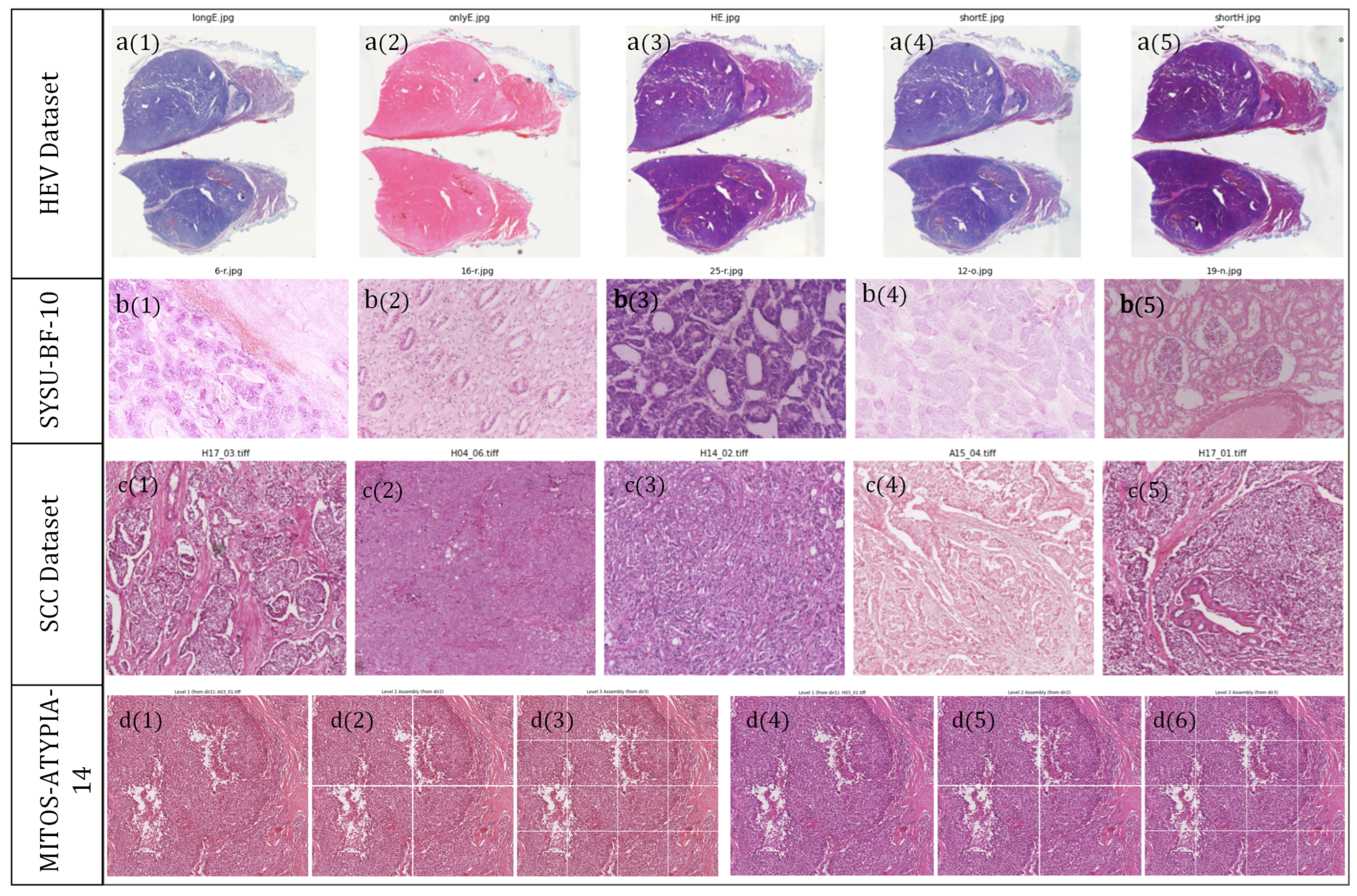
A summary of dataset characteristics and representative visualizations is provided in Table 1 and Figure 3.

Table 1. Summary of datasets used for experimental evaluation.

Dataset	#Cases	#WSIs	Magnification	Color Variation Source	Body Part
MITOS-14	14	28	40×/0.25 μm	Two imaging scanners	Breast
SCC dataset	44	220	40×/0.25 μm	Five imaging scanners	Skin
HEV dataset	1	9	40×/0.25 μm	Nine staining protocols	Thyroid
SYSU-BF-10	25	50	40×/0.25 μm	Color fading in 10 years	Breast

Figure 3. Representative examples from the four datasets. Row (a) shows selected staining protocols from the HEV dataset: (a1) longE, (a2) onlyE, (a3) H&E, (a4) shortE, and (a5) shortH. Row (b) shows five representative SYSU-BF-10 cases, with (b1–b5) denoting the displayed cases from left to right and illustrating long-term fading and temporal color drift. Row (c) shows SCC images acquired by five scanner/domain codes, with (c1–c5) corresponding to cs2, gt450, nz20, nz210, and p1000, respectively. Row (d) shows one MITOS-14 case at three magnification levels together with the corresponding cross-scanner control group; (d1–d6) denote the six displayed MITOS-14 panels from left to right.

6.1.2. Implementation Details

In surveying the literature on stain normalization, we observe that most existing methods are evaluated primarily on pre-extracted WSI tiles and are often positioned as a preprocessing step for downstream tasks, such as classification or segmentation. In contrast, the ultimate goal of digital pathology in the clinical setting is to provide pathologists with visually consistent slides, especially in cross-site, multi-center collaborations and remote diagnostic workflows. Under these scenarios, a robust and interpretable color normalization scheme at the whole-slide level is of central importance.

Motivated by this observation, we design our experiments to assess performance from two complementary perspectives:

1.

Full-resolution WSI normalization. We evaluate the behavior of each method when applied directly to entire, full-size histopathology slides.

2.

Tile-based reconstruction. We further consider the practically common pipeline in which a large WSI is first partitioned into tiles, normalized tile-wise, and then reassembled into a full-resolution slide. This setting is particularly relevant for memory-constrained or streaming-based deployments.

In addition to the four real-world datasets used in our study, we also construct a synthetic test image (synthetic_image) with controlled color and structural patterns. This synthetic benchmark provides an intuitive and stress-test-style assessment of robustness and generalization across a wide range of stain variations.

All experiments are conducted on a server equipped with an Intel(R) Xeon(R) Platinum 8352V CPU @ 2.10 GHz, an NVIDIA RTX 4090 GPU with 24 GB of VRAM, and 512 GB of system memory. The software stack is based on Python 3.8 and PyTorch 2.5.

6.1.3. Baselines

We compare the proposed method against three representative baselines:

• Reinhard. The classical global Reinhard color transfer algorithm [3] serves as our primary reference for global-statistics-based normalization. It matches low-order statistics between source and target images in a decorrelated color space and remains widely used in digital pathology.
• GCTI. We include a geometry-aware method with local alignment in the stain vector space (GCTI) [14], which explicitly exploits the underlying geometric structure of color distributions to compensate for scanner- and protocol-induced variations in microscopy images within a unified framework.
• CycleGAN. As a deep learning-based baseline, we employ a CycleGAN-style stain transfer model [19]. This method learns a non-linear mapping between source and target stain domains from unpaired data and represents a strong data-driven alternative to hand-crafted normalization schemes.

These baselines jointly cover global-statistics approaches, geometry-aware model-based methods, and modern generative adversarial networks, providing a comprehensive context for evaluating the proposed gradient-domain diffusion normalization.

6.2. Evaluation Metrics

In practice, there is still no widely accepted, unified standard for quantitative evaluation in the stain normalization task. Existing work typically adopts a mixture of structural similarity measures, color-space or gamut-based criteria, and performance gains on downstream tasks (e.g., classification or segmentation). From a clinical perspective, however, the ideal outcome is clear: the normalized image should (i) preserve the structural and morphological content of the source image and (ii) match the color space and distribution of the target image as closely as possible. Achieving this would allow pathology images acquired at different hospitals, regions, and from heterogeneous devices to be mapped to a common color standard, thereby reducing color-induced variability, improving diagnostic efficiency for pathologists, and ultimately promoting more standardized diagnostic criteria.

To better assess the performance of different algorithms under this perspective, we evaluate: (1) the structural similarity between the source image and the normalized result, and (2) the chromatic alignment between the normalized result and the target image. Concretely, we use the Structural Similarity Index (SSIM) [46] as a morphology-oriented metric between the source $I_S$ and the normalized image ${\tilde{I}}_S$, and the 1st-Wasserstein distance [47] between the color distributions of ${\tilde{I}}_S$ and the target $I_T$. Considering the entanglement of structure and color in the RGB space, all metrics are computed in the CIELab color space. The specific definitions are as follows.

• Structural Similarity Index (SSIM). To quantify the preservation of tissue morphology and local texture, we employ the SSIM metric. Let $\mathbf{x}$ and $\mathbf{y}$ denote local window patches extracted from the luminance channels of the source image $I_S$ and the normalized image ${\tilde{I}}_S$, respectively. The SSIM is defined as:

  $$\mathrm{SSIM}(\mathbf{x},\mathbf{y})={\displaystyle \frac{(2{\mu }_x{\mu }_y+C_1)(2{\sigma }_{xy}+C_2)}{({\mu }_x^2+{\mu }_y^2+C_1)({\sigma }_x^2+{\sigma }_y^2+C_2)}},$$

  (31)

  where ${\mu }_x,{\mu }_y$ represent the local means, ${\sigma }_x^2,{\sigma }_y^2$ denote the local variances, and ${\sigma }_{xy}$ is the cross-covariance between the two patches. The constants $C_1={\left(k_{1}L\right)}^2$ and $C_2={\left(k_{2}L\right)}^2$ are included to ensure numerical stability, where L is the dynamic range of pixel values (e.g., $L=255$ for 8-bit images). The final SSIM score is computed as the mean over all sliding windows in the image domain.

• Wasserstein Distance (W-D). To evaluate chromatic alignment, we calculate the 1st-Wasserstein distance (also known as Earth Mover’s Distance) between the color distributions of the target image $I_T$ and the result ${\tilde{I}}_S$. For a specific color channel $c\in \{a^{*},b^{*}\}$, let $P_c$ and $Q_c$ represent the probability distributions of pixel intensities in $I_T$ and ${\tilde{I}}_S$, respectively. The Wasserstein distance $W_1(P_c,Q_c)$ is defined as the minimal cost to transform one distribution into the other:

  $$W_1(P_c,Q_c)=\underset{\gamma \in \Pi (P_c,Q_c)}{inf}{\mathbb{E}}_{(u,v)\sim \gamma }\left[\right|u-v\left|\right],$$

  (32)

  where $\Pi (P_c,Q_c)$ denotes the set of all joint distributions $\gamma (u,v)$ whose marginals are $P_c$ and $Q_c$. Since we operate on 1D marginal distributions of color channels, Equation (32) has a closed-form solution expressed via the cumulative distribution functions (CDFs), $F_T\left(z\right)$ and $F_R\left(z\right)$:

  $$W_1(P_c,Q_c)={\int }_{-\infty }^{+\infty }|F_T\left(z\right)-F_R\left(z\right)|dz.$$

  (33)

  A lower $W_1$ score indicates superior alignment of the statistical color profile, without assuming Gaussianity of the underlying distributions.

6.3. Results and Visual Analysis

We complement the quantitative evaluation with a detailed visual comparison across four representative datasets and a synthetic benchmark. This analysis focuses on both full-size whole-slide views and tiled reconstructions.

6.3.1. Full Size Baseline Test

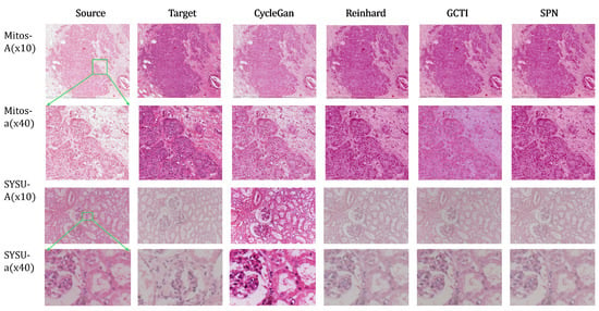
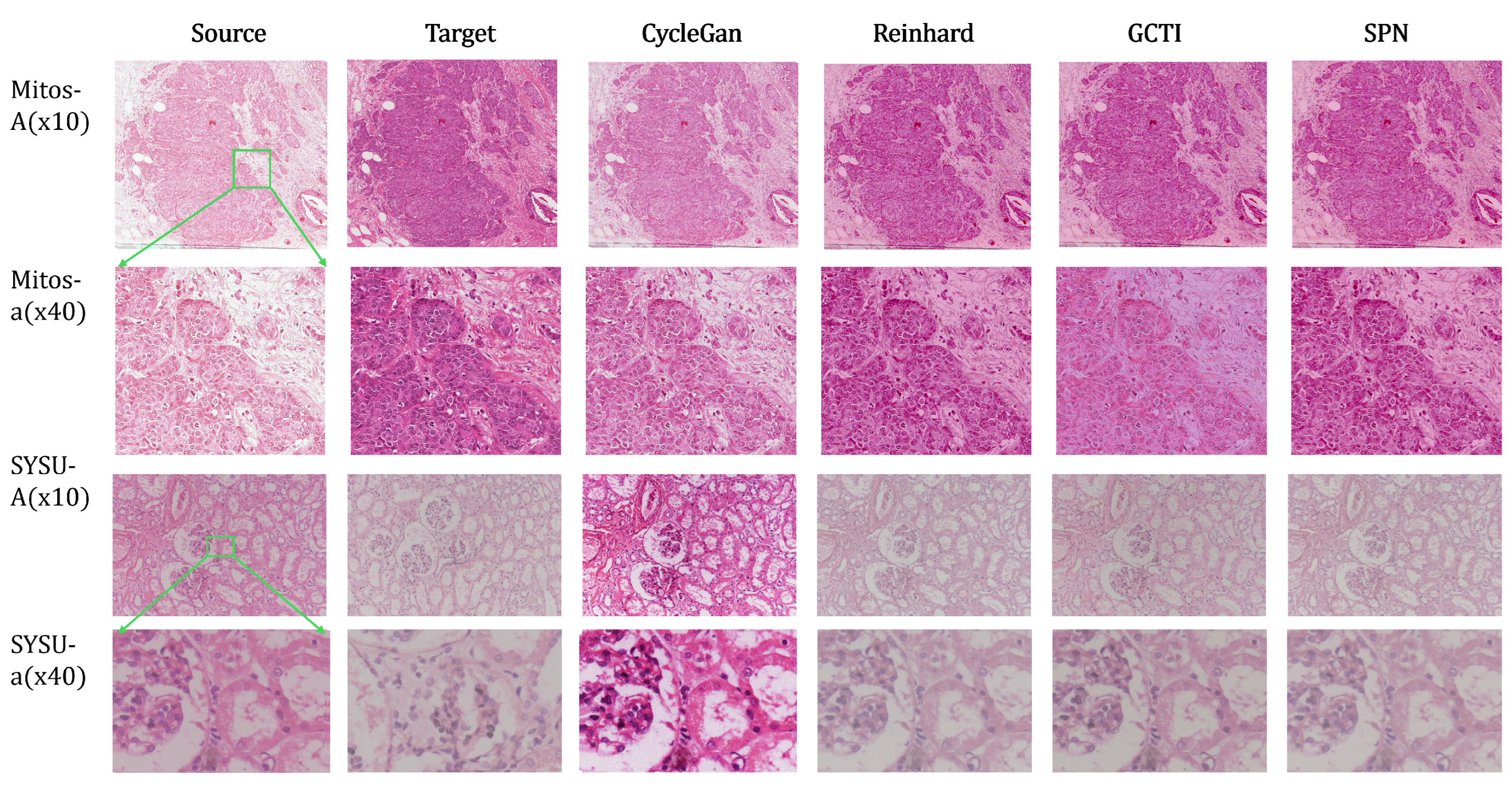
As illustrated in the first two rows of Figure 4, both Reinhard and SPN achieve faithful chromatic adaptation. This performance is consistent with their explicit statistical matching in the CIELab space, where the $a^{*}$ and $b^{*}$ channels isolate chromaticity from luminance. In contrast, the third and fourth rows reveal the limited generalization of CycleGAN on out-of-distribution data: when applied to non-MITOS samples, the model introduces a characteristic “deep red” bias inherent to its training set rather than correctly adapting to the target domain. Furthermore, compared to the global Reinhard method, SPN and GCTI preserve high-frequency morphological details, exhibiting significantly sharper cellular boundaries at high magnification.

Figure 4. Full-size results of different methods on the MITOS-14 and SYSU-BF-10 datasets. Normalization setup for the MITOS-14 (cross-scanner: Aperio to Hamamatsu, $10\times$/$40\times$) and SYSU-BF-10 (temporal drift: 10-year rescan) datasets. Note that the CycleGAN results are obtained using a model trained only on the MITOS-14 dataset.

6.3.2. SCC Dataset: Full-Size vs. Tiled Normalization

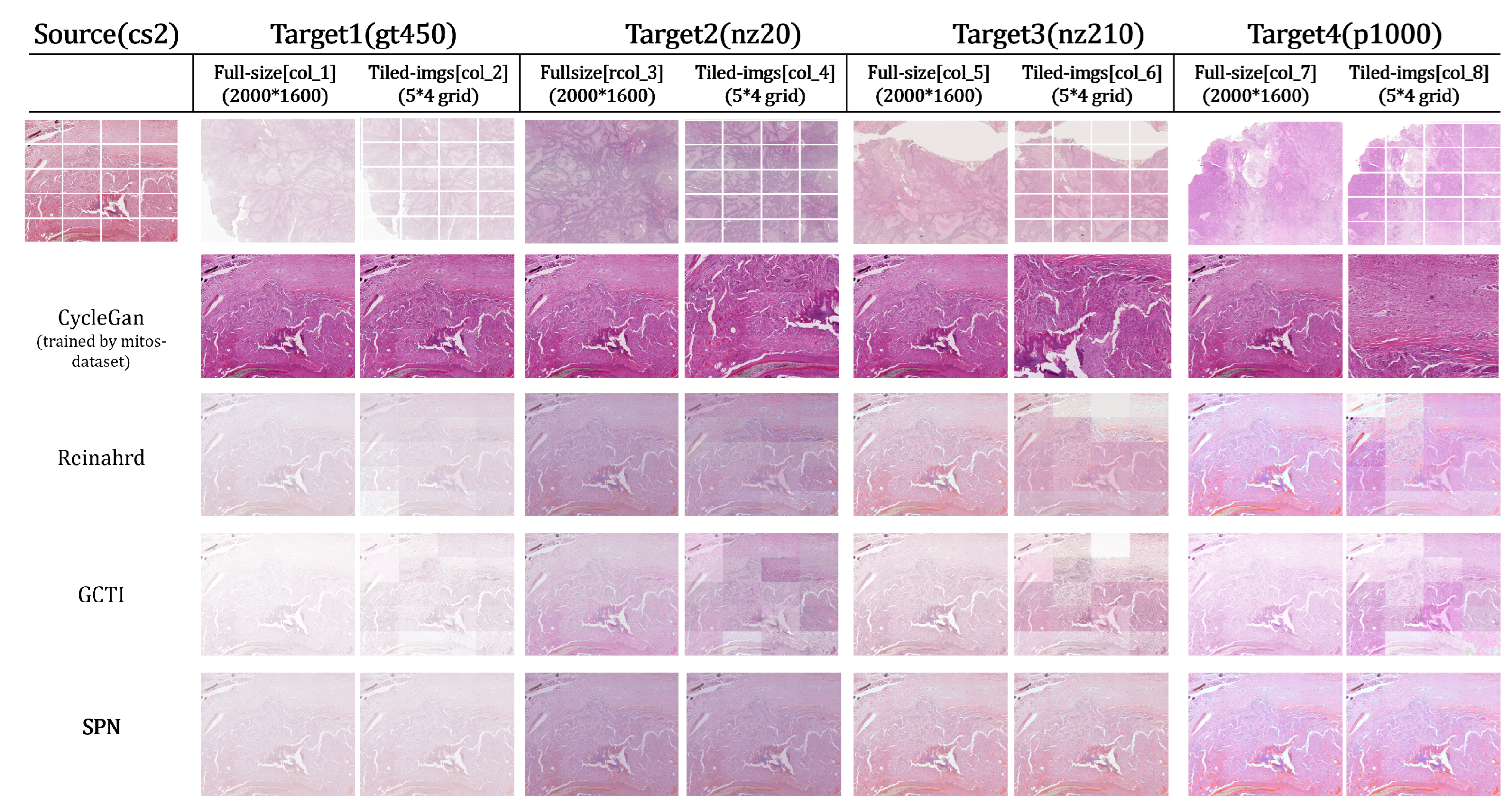
The SCC dataset contains slides acquired from five different scanners with codes cs2, gt450, nz20, nz210, and p1000. We use cs2 as the source device and treat the remaining four devices as distinct targets. Figure 5 compares color normalization on both full-size images and tiled images. The full-size resolution is $2000\times 1600$, and the tiled setting uniformly partitions each image into a $5\times 4$ grid of non-overlapping patches.

Figure 5. Full-size and tiled normalization results on the multi-scanner SCC dataset (cs2, gt450, nz20, nz210, p1000). Due to limited generalization outside the MITOS-14 training set, CycleGAN produces identical outputs across different target domains. We therefore display the base CycleGAN reconstruction in Column 2, with corresponding high-magnification details shown in col 4, 6, and 8.

As shown in Figure 5, tile-wise normalization via Reinhard and GCTI introduces distinct boundary discontinuities arising from inconsistent local statistics. While SPN effectively eliminates these seams through gradient preservation, CycleGAN displays a diminished checkerboard effect relative to the statistical methods. This partial suppression is attributed to the shared generator, which enforces a consistent color transform across tiles. Yet, this same mechanism limits adaptability, causing CycleGAN to hallucinate the MITOS style onto the SCC samples rather than respecting the target domain’s specific appearance.

6.3.3. HEV Dataset: Multi-Stained Pathology Images

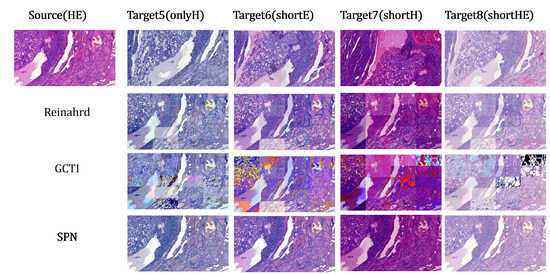
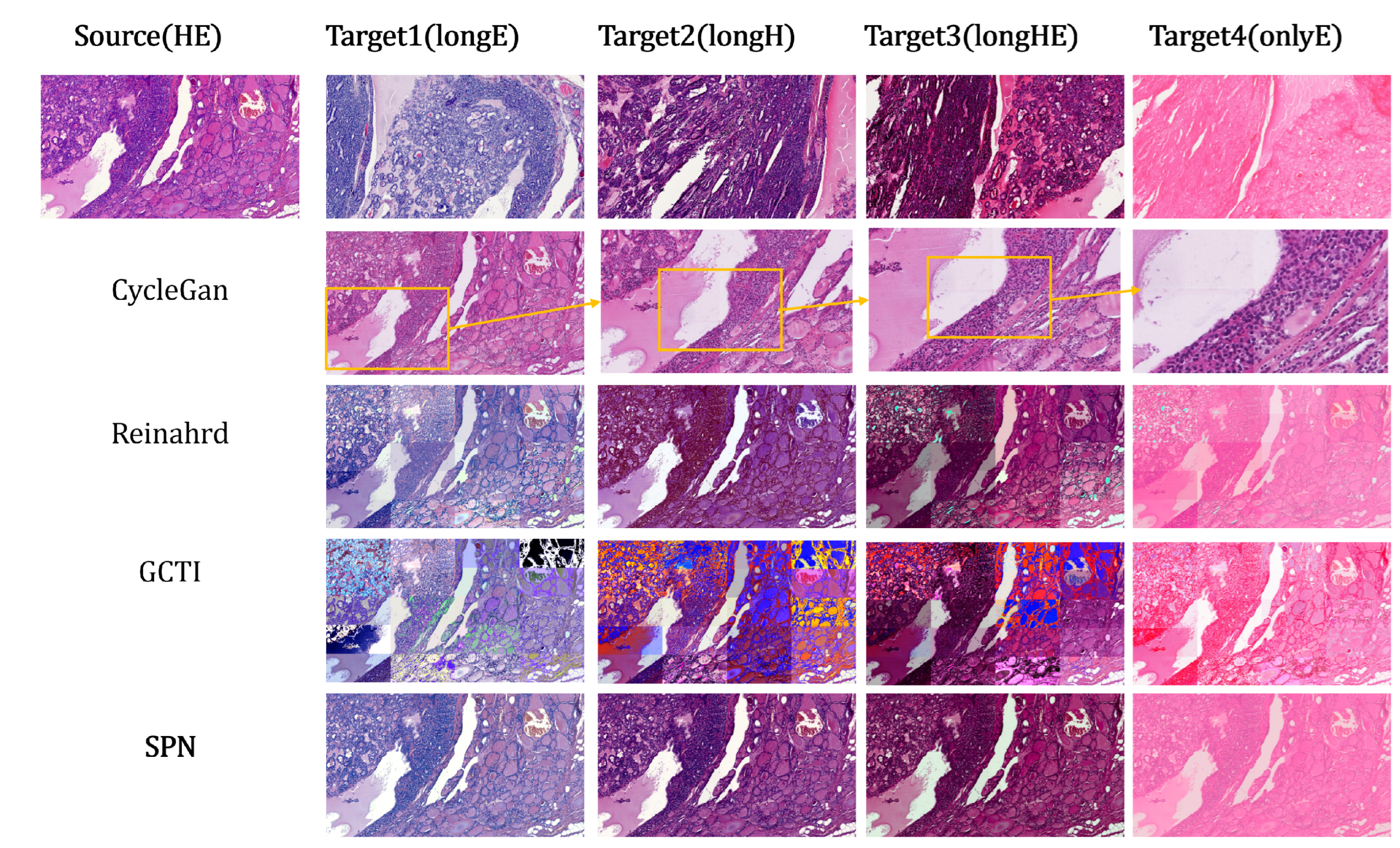
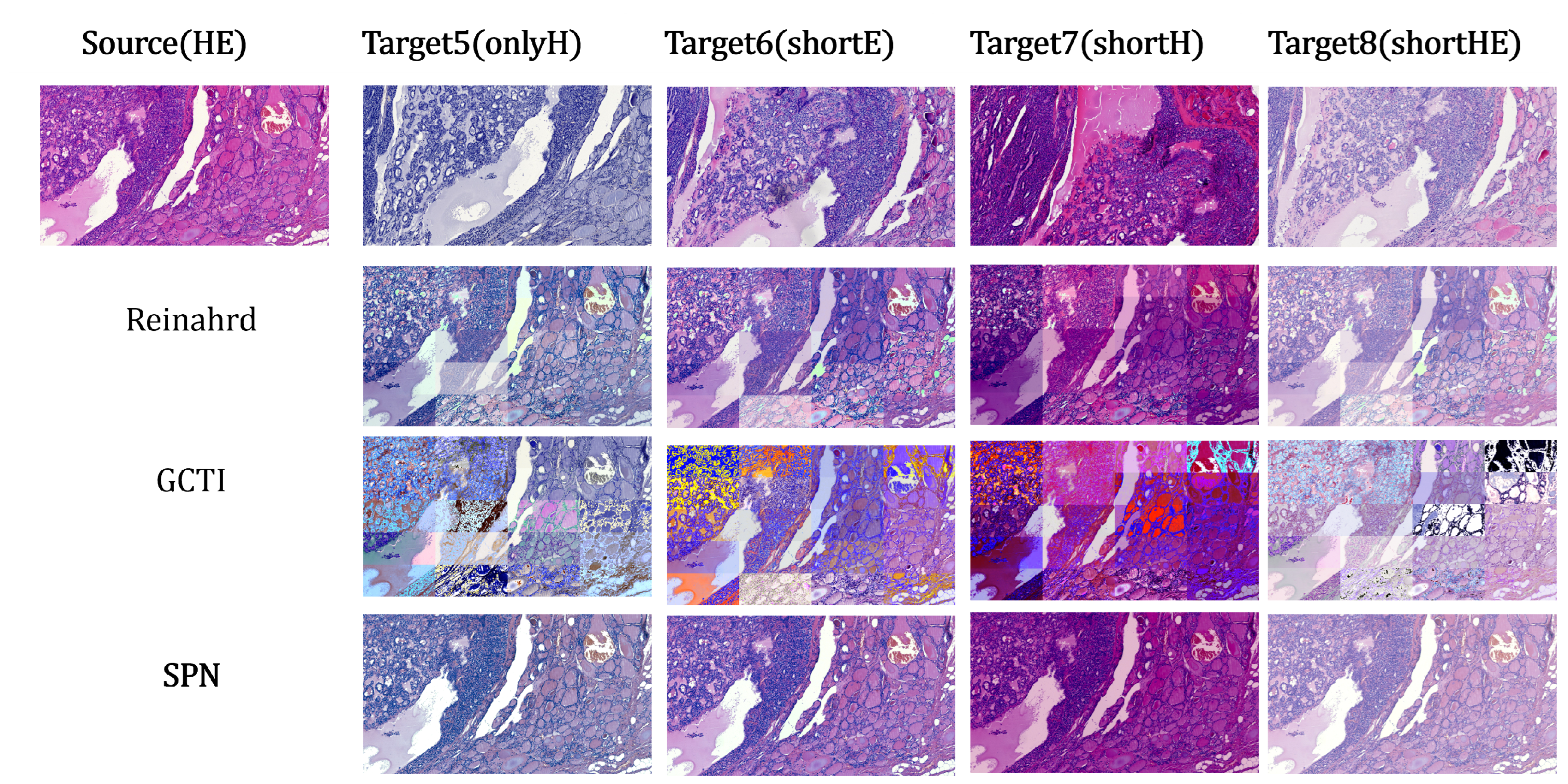
The HEV dataset encompasses nine distinct staining configurations, offering the richest color diversity among the datasets analyzed. We utilize standard HE as the source domain, treating the remaining eight protocols as targets. For brevity, and because full-slide comparisons show limited variation, Figure 6 focuses exclusively on the tiled results.

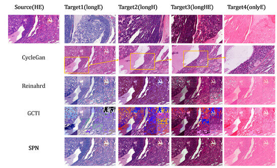
Figure 6. Tiled-image results of different methods on the HEV dataset. The CycleGAN model is still trained on MITOS-14, leading to nearly identical outputs across the eight HEV targets; we therefore show a single CycleGAN row with selected regions magnified.

The CycleGAN results in Figure 6 mirror those in Figure 5: blocking artifacts are diminished relative to Reinhard and GCTI due to the global constraints of the generator. More significantly, this experiment highlights the robustness limitations of the GCTI framework. GCTI employs a local wedge-finding algorithm that projects pixel intensities onto a subspace defined by SVD, inferring stain vectors via angular percentiles (e.g., 0.1th and 99.9th). This mechanism is susceptible to failure in extreme scenarios: (1) illumination correction singularities, where near-zero background estimates lead to division-by-zero errors and intensity saturation, and (2) thresholding instability in uniform regions, where the lack of color variance renders percentile-based thresholds arbitrary. Figure 6 clearly demonstrates the former, where instability in the background estimation step produces extensive artifacts characterized by signal saturation and loss of texture.

6.3.4. Evaluation on Synthetic Image

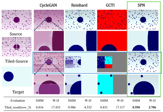
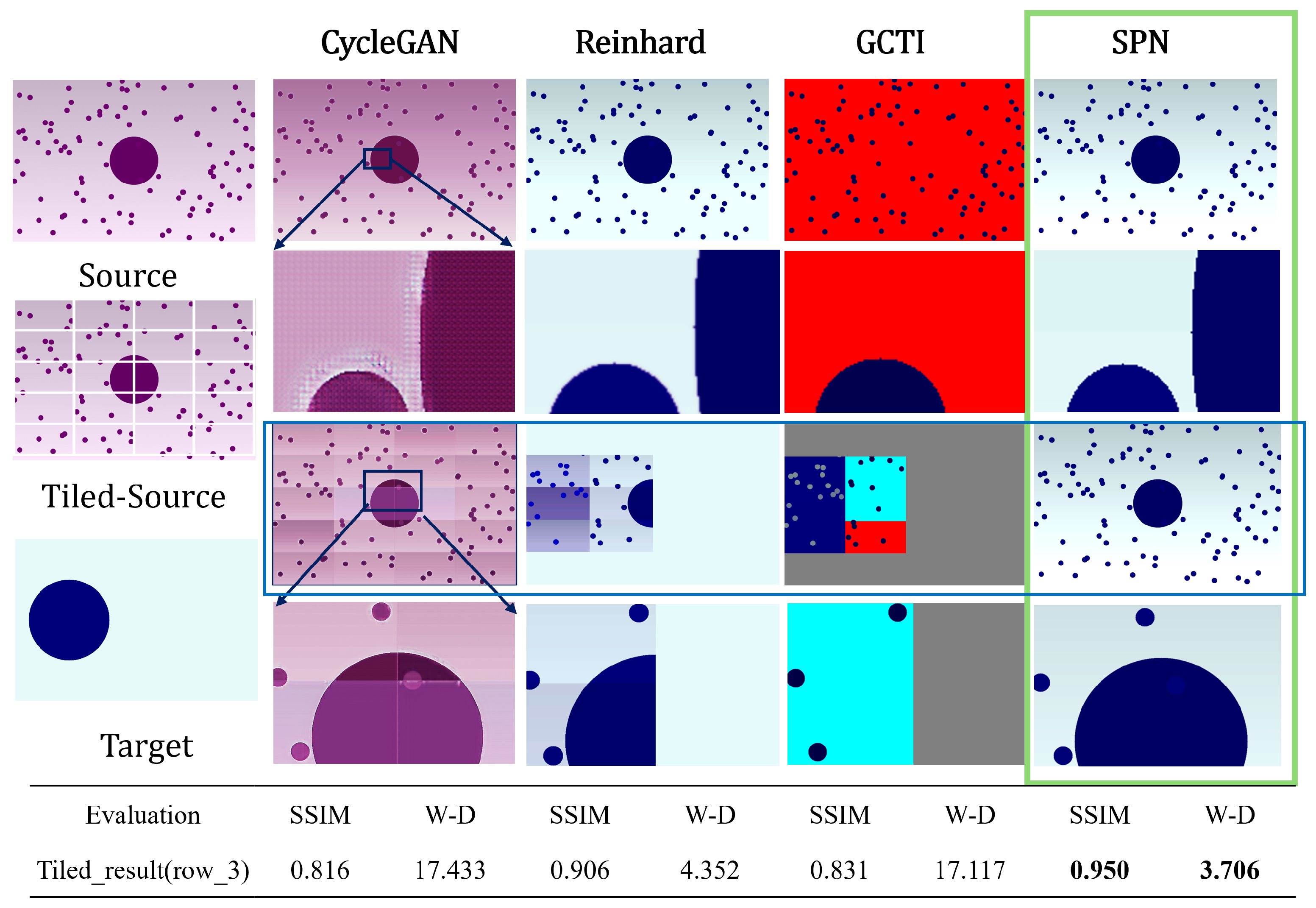
To rigorously assess algorithmic stability under limiting conditions, we introduce a synthetic image characterized by a smooth background gradient and a central geometric object (Figure 7).

Figure 7. Robustness evaluation on the synthetic image. The blue-framed row is the main comparison quantified below; the green-framed column marks the best result (SPN). Row 1: Full-resolution normalization. SPN preserves the background gradient faithfully. GCTI exhibits a division-by-zero singularity due to background misclassification, causing saturation. Rows 2–3: Tiled reconstruction using a non-overlapping grid. The CycleGAN model is trained on MITOS-14. Reinhard fails on homogeneous tiles where statistical moments are undefined, and GCTI suffers from rank deficiency in zero-gradient regions (pure background). Tiles where an algorithm fails to converge are masked in gray.

The first row of Figure 7 presents the full-resolution normalization results. SPN and Reinhard achieve the most faithful reconstruction of the background gradient, demonstrating robust structural consistency across both low-frequency trends and high-frequency edges. In contrast, GCTI exhibits a catastrophic failure mode driven by algorithmic instability: the central large circle is misclassified as background, causing the denominator in the illumination correction step to approach zero. This singularity leads to numerical explosion, resulting in a saturated, near-uniform output in the background region.

Additionally, the magnified regions in the second row reveal that CycleGAN produces spurious ringing artifacts around the circular structures, a phenomenon inconsistent with the behavior of the variational and statistical methods. This artifact stems from the generative network’s reliance on learned upsampling filters (transposed convolutions) which, unlike rigorous interpolation schemes, can hallucinate high-frequency noise to satisfy the discriminator. Such artifacts underscore the critical deficit of deep generative models regarding interpretability: unlike the proposed framework, which is constrained by a physical diffusion process, the GAN introduces opaque, architectural artifacts that compromise diagnostic confidence. The tiled results (Row 3) further expose the stability limits of the baseline methods, particularly regarding well-posedness on disjoint subdomains. First, statistical methods break down on homogeneous patches. Reinhard normalization relies on matching first- and second-order moments; when a target tile consists of a pure background (zero variance), the scaling factors become undefined, rendering the transfer function ill-posed. Similarly, GCTI fails in these homogeneous regions because the lack of spectral diversity renders the SVD-based stain estimation rank-deficient, leading to numerical breakdown.

Conversely, SPN maintains both global gradient continuity and local geometric fidelity across all tiles. This robustness confirms that the proposed variational framework effectively regularizes the normalization problem, preventing the degenerate behavior observed in purely statistical approaches when local data is sparse.

6.4. Quantitative Results and Discussion

Table 2 presents a comprehensive quantitative comparison of our proposed SPN against three state-of-the-art methods: CycleGAN, Reinhard, and GCTI. We utilize the Structural Similarity Index Measure (SSIM) to evaluate structure preservation (↑) and the Wasserstein distance (W-D) to assess stain distribution matching (↓).

Table 2. Quantitative comparison of different stain normalization methods. The best results (max SSIM and min W-D) for each row are highlighted in bold.

Dataset	Pair	CycleGAN †		Reinhard		GCTI		SPN (Ours)
		SSIM ↑	W-D ↓	SSIM ↑	W-D ↓	SSIM ↑	W-D ↓	SSIM ↑	W-D ↓
SYSU-BF	18-n → o	0.742	18.572	0.981	0.751	0.970	1.104	0.875	0.689
mitos-14	A06_01 → H	0.790	7.274	0.911	2.558	0.813	7.042	0.822	3.027
HEV data	HE → longE	0.957	15.392	0.920	4.280	0.736	6.338	0.983	3.524
	HE → onlyE	–	12.134	0.729	2.464	0.832	6.485	0.718	1.940
	HE → shortE	–	11.902	0.932	5.577	0.832	13.999	0.992	3.705
	HE → longHE	–	5.892	0.765	3.370	0.656	10.915	0.814	4.255
	HE → onlyH	–	18.802	0.920	2.540	0.634	4.427	0.979	3.672
	HE → shortHE	–	15.113	0.873	3.488	0.667	4.096	0.896	3.118
	HE → longH	–	4.792	0.875	4.745	0.755	22.539	0.921	2.146
	HE → shortH	–	13.199	0.825	2.918	0.694	13.107	0.857	3.218
SCC data	cs2 → gt450	0.921	25.624	0.679	0.495	0.757	1.873	0.641	0.360
	cs2 → nz20	–	20.885	0.838	0.801	0.898	1.950	0.882	1.715
	cs2 → nz210	–	16.042	0.880	0.524	0.917	2.074	0.827	0.581
	cs2 → p1000	–	10.979	0.886	1.022	0.798	4.310	0.912	1.579
synthetic_image		0.816	17.433	0.906	4.352	0.831	17.117	0.950	3.706

^† CycleGAN model trained on the MITOS-14 dataset. Since SSIM is calculated between result and source image, for the same source test, we omit meaningless comparisons using “–”.

It is worth noting that the classic Reinhard and GCTI algorithms remain strong baselines, particularly on relatively simple and highly structured datasets such as SYSU-BF-10 and MITOS-14. In these cases, Reinhard achieves competitive or even state-of-the-art results (e.g., SSIM of 0.981 on SYSU-BF-10). This is likely because these datasets exhibit unimodal color distributions where simple global statistical alignment (mean and standard deviation matching) is sufficient. However, its performance degrades significantly on complex datasets like HEV (W-D often $>4.0$), where stain variations are non-linear and multi-modal.

As previously discussed, CycleGAN utilizes fixed weights trained on MITOS. While it yields consistent structural outputs (omitted entries in Table 2), its inability to adapt to the specific target reference leads to large domain discrepancies, evidenced by high W-D scores (e.g., 25.624 on SCC).

Our method demonstrates robust performance across diverse scenarios, with its advantages becoming most pronounced on the synthetic_image. This dataset serves as a rigorous benchmark for “general stain normalization” as it provides paired ground truth. On this set, SPN achieves the best results in both metrics (SSIM: 0.950, W-D: 3.706). This controlled result supports the numerical robustness of the proposed screened variational formulation under strong homogeneous and tiled perturbations, where local statistical or factorization-based methods may become unstable.

6.5. Discussion and Perspectives

The quantitative and visual results indicate that the relative advantage of a normalization method depends strongly on the type of stain variation. On simpler two-domain settings, where the chromatic mismatch is predominantly global and the target distribution is close to unimodal, classical statistical normalization remains highly effective; this is consistent with the strong performance of Reinhard on SYSU-BF-10 and MITOS-14. The benefit of SPN becomes more apparent when stain variation is spatially heterogeneous, when local statistics become unreliable, or when normalization must be performed and reassembled at whole-slide scale. In these regimes, the screened Poisson formulation provides a stable compromise between structural fidelity and chromatic transfer, and the SCC tiled experiments show that the localization result in Section 4 has direct numerical value for seamless full-slide reconstruction.

The comparison also clarifies the respective weaknesses of the baseline methods. Reinhard is efficient and competitive for global color shifts, but its purely global transform may weaken local microstructure and offers no intrinsic control of tile-interface consistency. GCTI incorporates stain geometry and local statistics, yet its SVD/NMF-based estimation can become unstable in homogeneous, background-dominated, or low-rank regions, as reflected in the HEV and synthetic tests. Learning-based transfer methods, such as CycleGAN, can model nonlinear appearance changes, but their reliability depends on the coverage of the training distribution and may degrade under domain mismatch through style bias or generative artifacts. SPN avoids training dependence and remains stable under tiled whole-slide processing, but it is not free of limitations: it still requires a reference target and a small set of model parameters, and the present study has been restricted mainly to H&E-like staining conditions.

From an application perspective, the whole-slide experiments indicate that SPN can produce globally coherent normalized slides that remain visually consistent after tile-wise reconstruction, rather than merely providing patch-level outputs for subsequent models. This is important in digital pathology, where stain normalization is expected to support both direct visual assessment by pathologists and standardized input for downstream computational analysis. The current formulation is centered on reference-based normalization in H&E-like settings, and several natural extensions remain open, including broader multi-center evaluation, reader-oriented assessment, downstream studies on tasks such as classification and segmentation, and generalization to more complex multi-stain scenarios. These directions also suggest hybrid pipelines in which SPN acts either as a deterministic whole-slide normalization module or as a mathematically constrained component within learning-based pathology systems.

7. Conclusions

We have presented Screened Poisson Normalization (SPN), a variational stain-normalization framework derived from the steady-state reaction–diffusion interpretation of histological staining. By coupling gradient-domain structural fidelity with chromatic anchoring in the CIE $L^{*}{a}^{*}{b}^{*}$ space, the method yields an interpretable screened Poisson model that admits rigorous analysis and a full-slide numerical implementation. The theoretical results establish a stable mathematical basis for the model, while the localization property of the screened operator enables a non-overlapping tiled solver for gigapixel whole-slide images.

On H&E pathology data, including scanner variation, staining-protocol variation, archival fading, and synthetic stress testing, SPN shows that it can preserve diagnostically relevant morphology while achieving coherent color normalization at full-slide scale. A particularly important outcome of this work is that the tile-wise implementation remains consistent after reassembly, producing visually seamless whole-slide results without heuristic overlap blending. This makes the framework relevant not only for patch-level preprocessing in computational pathology, but also for the direct generation of globally normalized slides for clinical viewing.

The present study is limited to H&E-like staining, and broader validation remains necessary. In future work, we plan to extend the SPN framework to more complex multi-stain scenarios, including immunohistochemistry (IHC) and multiplex immunohistochemistry, where channel interactions and stain cross-talk are richer than in standard H&E. Another natural direction is to combine SPN with downstream deep learning and intelligent-diagnosis pipelines, either as a deterministic normalization front-end or as a mathematically guided regularization component. We expect these developments to support broader clinical testing and to further clarify the role of stain normalization in robust computational pathology.

References

- Xu, C.; Sun, Y.; Zhang, Y.; Liu, T.; Wang, X.; Hu, D.; Huang, S.; Li, J.; Zhang, F.; Li, G. Stain Normalization of Histopathological Images Based on Deep Learning: A Review. Diagnostics 2025, 15, 1032. [Google Scholar] [CrossRef] [Scilit]
- Gurina, T.S.; Simms, L. Histology, Staining. In StatPearls [Internet]; StatPearls Publishing: Treasure Island, FL, USA, 2023. [Google Scholar]
- Reinhard, E.; Ashikhmin, M.; Gooch, B.; Shirley, P. Color transfer between images. IEEE Comput. Graph. Appl. 2001, 21, 34–41. [Google Scholar] [CrossRef] [Scilit]
- Zarella, M.D.; Yeoh, C.; Breen, D.E.; Garcia, F.U. An alternative reference space for H&E color normalization. PLoS ONE 2017, 12, e0174489. [Google Scholar]
- Magee, D.; Treanor, D.; Crellin, D.; Shires, M.; Smith, K.; Mohee, K.; Quirke, P. Colour normalisation in digital histopathology images. In Proceedings of Optical Tissue Image Analysis in Microscopy, Histopathology and Endoscopy (MICCAI Workshop); Daniel Elson: London, UK, 2009; pp. 100–111. [Google Scholar]
- Li, Y.; Zhou, H.; Liu, N.; Shen, Y. Stain normalization and augmentation in frequency space for histology analysis. In Proceedings of the 2023 IEEE International Conference on Bioinformatics and Biomedicine (BIBM), Istanbul, Turkiye, 5–8 December 2023; pp. 2031–2035. [Google Scholar]
- Roy, S.; Lal, S.; Kini, J.R. Novel color normalization method for Hematoxylin & Eosin stained histopathology images. IEEE Access 2019, 7, 28982–28998. [Google Scholar] [CrossRef] [Scilit]
- Vijh, S.; Saraswat, M.; Kumar, S. A new complete color normalization method for H&E stained histopathological images. Appl. Intell. 2021, 51, 1–14. [Google Scholar]
- Nadeem, S.; Hollmann, T.; Tannenbaum, A. Multimarginal Wasserstein barycenter for stain normalization and augmentation. In International Conference on Medical Image Computing and Computer-Assisted Intervention (MICCAI); Springer International Publishing: Cham, Switzerland, 2020; pp. 362–371. [Google Scholar]
- Macenko, M.; Niethammer, M.; Marron, J.S.; Borland, D.; Woosley, J.T.; Guan, X.; Schmitt, C.; Thomas, N.E. A method for normalizing histology slides for quantitative analysis. In Proceedings of the 2009 IEEE International Symposium on Biomedical Imaging: From Nano to Macro, Boston, MA, USA, 28 June–1 July 2009; pp. 1107–1110. [Google Scholar]
- Vahadane, A.; Peng, T.; Sethi, A.; Albarqouni, S.; Wang, L.; Baust, M.; Steiger, K.; Schlitter, A.M.; Esposito, I.; Navab, N. Structure-preserving color normalization and sparse stain separation. IEEE Trans. Med. Imaging 2016, 35, 1962–1971. [Google Scholar] [CrossRef] [Scilit] [PubMed]
- Zheng, Y.; Jiang, Z.; Zhang, H.; Xie, F.; Shi, J.; Xue, C. Adaptive color deconvolution for histological WSI normalization. Comput. Methods Programs Biomed. 2019, 170, 107–120. [Google Scholar] [CrossRef] [Scilit]
- Alsubaie, N.; Trahearn, N.; Raza, S.E.A.; Snead, D.; Rajpoot, N.M. Stain deconvolution using statistical analysis of multi-resolution stain colour representation. PLoS ONE 2017, 12, e0169875. [Google Scholar] [CrossRef] [Scilit] [PubMed]
- Gupta, A.; Duggal, R.; Gehlot, S.; Gupta, R.; Mangal, A.; Kumar, L.; Thakkar, N.; Satpathy, D. GCTI-SN: Geometry-inspired chemical and tissue invariant stain normalization of microscopic medical images. Med. Image Anal. 2020, 65, 101788. [Google Scholar] [CrossRef] [Scilit]
- Tellez, D.; Litjens, G.; Bándi, P.; Bulten, W.; Bokhorst, J.-M.; Ciompi, F.; van der Laak, J. Quantifying the effects of data augmentation and stain color normalization in convolutional neural networks for computational pathology. Med. Image Anal. 2019, 58, 101544. [Google Scholar] [CrossRef] [Scilit] [PubMed]
- Kang, H.; Luo, D.; Feng, W.; Zeng, S.; Quan, T.; Hu, J.; Liu, X. StainNet: A fast and robust stain normalization network. Front. Med. 2021, 8, 746307. [Google Scholar] [CrossRef] [Scilit]
- Lee, C.C.; Kuo, P.T.P.; Peng, C.H. H&E stain normalization using U-net. In Proceedings of the 2022 IEEE 22nd International Conference on Bioinformatics and Bioengineering (BIBE), Virtual, 7–9 November 2022; pp. 29–32. [Google Scholar]
- Wang, C.; Li, S.; Ke, J.; Zhang, C.; Shen, Y. RandStainNA++: Enhance random stain augmentation and normalization through foreground and background differentiation. IEEE J. Biomed. Health Inform. 2024, 28, 3660–3671. [Google Scholar] [CrossRef] [Scilit]
- Runz, M.; Rusche, D.; Schmidt, S.; Weihrauch, M.R.; Hesser, J.; Weis, C.A. Normalization of H&E-stained histological images using cycle consistent generative adversarial networks. Diagn. Pathol. 2021, 16, 71. [Google Scholar]
- Shaban, M.T.; Baur, C.; Navab, N.; Albarqouni, S. Staingan: Stain style transfer for digital histological images. In Proceedings of the 2019 IEEE 16th International Symposium on Biomedical Imaging (ISBI 2019), Venice, Italy, 8–11 April 2019; pp. 953–956. [Google Scholar]
- BenTaieb, A.; Hamarneh, G. Adversarial stain transfer for histopathology image analysis. IEEE Trans. Med. Imaging 2017, 37, 792–802. [Google Scholar] [CrossRef] [Scilit]
- Shrivastava, A.; Adorno, W.; Sharma, Y.; Ehsan, L.; Ali, S.A.; Moore, S.R.; Amadi, B.; Kelly, P.; Syed, S.; Brown, D.E. Self-attentive adversarial stain normalization. In Pattern Recognition. ICPR Workshops and Challenges; Springer: Berlin/Heidelberg, Germany, 2021; pp. 120–140. [Google Scholar]
- Cong, C.; Liu, S.; Di Ieva, A.; Pagnucco, M.; Berkovsky, S.; Song, Y. Colour adaptive generative networks for stain normalisation of histopathology images. Med. Image Anal. 2022, 82, 102580. [Google Scholar] [CrossRef] [Scilit] [PubMed]
- Nishar, H.; Chavanke, N.; Singhal, N. Histopathological stain transfer using style transfer network with adversarial loss. In Proceedings of the International Conference on Medical Image Computing and Computer-Assisted Intervention, Lima, Peru, 4–8 October 2020; pp. 330–340. [Google Scholar]
- Cho, H.; Lim, S.; Choi, G.; Min, H. Neural stain-style transfer learning using GAN for histopathological images. arXiv 2017, arXiv:1710.08543. [Google Scholar] [CrossRef] [Scilit]
- Liang, H.; Plataniotis, K.N.; Li, X. Stain style transfer of histopathology images via structure-preserved generative learning. In Machine Learning for Medical Image Reconstruction; Springer: Berlin/Heidelberg, Germany, 2020; pp. 153–162. [Google Scholar]
- Jeong, J.; Kim, K.D.; Nam, Y.; Cho, C.E.; Go, H.; Kim, N. Stain normalization using score-based diffusion model through stain separation and overlapped moving window patch strategies. Comput. Biol. Med. 2023, 152, 106335. [Google Scholar] [CrossRef] [Scilit]
- Kausar, T.; Kausar, A.; Ashraf, M.A.; Siddique, M.F.; Wang, M.; Sajid, M.; Siddique, M.Z.; Haq, A.U.; Riaz, I. SA-GAN: Stain acclimation generative adversarial network for histopathology image analysis. Appl. Sci. 2021, 12, 288. [Google Scholar] [CrossRef] [Scilit]
- Baykal Kablan, E. Regional realness-aware generative adversarial networks for stain normalization. Neural Comput. Appl. 2023, 35, 17915–17927. [Google Scholar] [CrossRef] [Scilit]
- Hetz, M.J.; Bucher, T.C.; Brinker, T.J. Multi-domain stain normalization for digital pathology: A cycle-consistent adversarial network for whole slide images. Med. Image Anal. 2024, 94, 103149. [Google Scholar] [CrossRef] [Scilit]
- Salvi, M.; Caputo, A.; Balmativola, D.; Scotto, M.; Pennisi, O.; Michielli, N.; Mogetta, A.; Molinari, F.; Fraggetta, F. Impact of stain normalization on pathologist assessment of prostate cancer: A comparative study. Cancers 2023, 15, 1503. [Google Scholar] [CrossRef] [Scilit]
- Hoque, M.Z.; Keskinarkaus, A.; Nyberg, P.; Seppänen, T. Stain normalization methods for histopathology image analysis: A comprehensive review and experimental comparison. Inf. Fusion 2024, 102, 101997. [Google Scholar] [CrossRef] [Scilit]
- Pérez, P.; Gangnet, M.; Blake, A. Poisson image editing. In Seminal Graphics Papers: Pushing the Boundaries; ACM: New York, NY, USA, 2023; Volume 2, pp. 577–582. [Google Scholar]
- Habring, A.; Holler, M. Neural-network-based regularization methods for inverse problems in imaging. GAMM-Mitteilungen 2024, 47, e202470004. [Google Scholar] [CrossRef] [Scilit]
- Mayerhöfer, T.G.; Pahlow, S.; Popp, J. The Bouguer-Beer-Lambert law: Shining light on the obscure. ChemPhysChem 2020, 21, 2029–2046. [Google Scholar] [CrossRef] [Scilit] [PubMed]
- Murray, J.D. Mathematical Biology I: An Introduction, 3rd ed.; Springer: New York, NY, USA, 2002. [Google Scholar]
- Menning, J.D.M.; Wallmersperger, T.; Meinhardt, M.; Ehrenhofer, A. Modeling and simulation of diffusion and reaction processes during the staining of tissue sections on slides. Histochem. Cell Biol. 2022, 158, 137–148. [Google Scholar] [CrossRef] [Scilit] [PubMed]
- Suvarna, K.S.; Layton, C.; Bancroft, J.D. (Eds.) Bancroft’s Theory and Practice of Histological Techniques, 8th ed.; Elsevier: Amsterdam, The Netherlands, 2019. [Google Scholar]
- Landini, G.; Martinelli, G.; Piccinini, F. Colour deconvolution: Stain unmixing in histological imaging. Bioinformatics 2021, 37, 1485–1487. [Google Scholar] [CrossRef] [Scilit]
- Fortunato, D.; Townsend, A. Fast Poisson solvers for spectral methods. IMA J. Numer. Anal. 2020, 40, 1994–2018. [Google Scholar] [CrossRef] [Scilit]
- Bressloff, P.C. Cellular diffusion processes in singularly perturbed domains. J. Math. Biol. 2024, 89, 58. [Google Scholar] [CrossRef] [Scilit]
- Klawonn, A.; Lanser, M.; Weber, J. Machine learning and domain decomposition methods—A survey. Comput. Sci. Eng. 2024, 1, 2. [Google Scholar] [CrossRef] [Scilit]
- Roux, L.; Racoceanu, D.; Loménie, N.; Kulikova, M.; Irshad, H.; Klossa, J.; Capron, F.; Genestie, C.; Le Naour, G.; Gurcan, M.N. Mitosis detection in breast cancer histological images: An ICPR 2012 contest. J. Pathol. Inform. 2013, 4, 8. [Google Scholar]
- Wilm, F.; Fragoso, M.; Bertram, C.A.; Stathonikos, N.; Öttl, M.; Qiu, J.; Klopfleisch, R.; Maier, A.; Breininger, K.; Aubreville, M. Multi-scanner canine cutaneous squamous cell carcinoma histopathology dataset. arXiv 2023, arXiv:2301.04423. [Google Scholar] [CrossRef] [Scilit]
- Runz, M.; Weis, C.-A. Normalization of HE-Stained Histological Images Using Cycle Consistent Generative Adversarial Networks [Dataset]. heiDATA, V1. 2021. Available online: https://heidata.uni-heidelberg.de/dataset.xhtml?persistentId=doi:10.11588/DATA/8LKEZF (accessed on 2 June 2025).
- Bakurov, I.; Buzzelli, M.; Schettini, R.; Castelli, M.; Vanneschi, L. Structural similarity index (SSIM) revisited: A data-driven approach. Expert Syst. Appl. 2022, 189, 116087. [Google Scholar] [CrossRef] [Scilit]
- Nguyen, K.; Ho, N. Revisiting sliced Wasserstein on images: From vectorization to convolution. Adv. Neural Inf. Process. Syst. 2022, 35, 17788–17801. [Google Scholar]
Disclaimer/Publisher’s Note: The statements, opinions and data contained in all publications are solely those of the individual author(s) and contributor(s) and not of MDPI and/or the editor(s). MDPI and/or the editor(s) disclaim responsibility for any injury to people or property resulting from any ideas, methods, instructions or products referred to in the content. |
© 2026 by the authors. Licensee MDPI, Basel, Switzerland. This article is an open access article distributed under the terms and conditions of the Creative Commons Attribution (CC BY) license.