Finite-Time Neural Adaptive Control of Electro-Hydraulic Servo Systems with Minimal Input Delay and Parametric Uncertainty via Padé Approximation

Abstract

Physical coupling, nonlinearity and uncertainty degrade the dynamic performance of electro-hydraulic servo systems, particularly under conditions involving input delays, leading to reduced trajectory tracking accuracy or even system instability. These factors often fail to meet the high-precision requirements of engineering applications. To effectively address these difficulties, this paper proposes a novel adaptive control protocol for networked electro-hydraulic servo systems. For the minimal communication delay problem of networked electro-hydraulic servo systems, Laplace transform algorithm together with Padé approximation is adopted in this study to remove the delay term from the mathematical system model. Moreover, the matched modeling parametric uncertainty of systems is estimated and compensated by the neural network adaptive method to improve the dynamical performance of the system during the steady state. The controller is designed on the basis of recursive backstepping strategy and the finite-time stability theorem, which can handle system nonlinearity and guarantee transient response. The validity of the proposed theoretical results is proved by Lyapunov stability and the feasibility and superiority are verified via physical simulation.

1. Introduction

Electro-hydraulic servo systems (EHSs) are precision control systems that integrate electrical control with hydraulic transmission. Due to their high accuracy, high power density, rapid response and robust load-driving capability, they are widely applied in control domains such as hydraulic manipulators [1], aircraft servo mechanisms [2], load simulators [3], and exoskeletons [4]. In recent years, in the context of industrial equipment that demands higher precision and faster response, many scholars have explored fields that include nonlinear systems [5], parameter perturbations [6], external disturbances [7], and Serpentine Manipulators [8]. EHSs also pose higher demands on control technologies. Therefore, enhancing the system’s tracking accuracy, interference resistance, and parameter adaptive adjustment capabilities to accommodate complex operating conditions has become a key research focus.

In the field of system dynamics research, classical theoretical systems typically take core characteristics including nonlinearity, time-variation, coupling and uncertainty as the starting point to establish systems for describing and analyzing complex physical systems. For these core characteristics, researchers have proposed various control schemes, including backstepping [9], adaptive control [10], PID control [11] and sliding mode variable structure control [12], which have laid a solid mathematical foundation for the control research of complex physical systems. In the field of robotics, numerous engineering applications exhibit inherent nonlinear behaviors. To improve the accuracy and efficiency of nonlinear motion control, Wang et al. proposed a trajectory planning scheme based on the generalized Jacobian operator [13]. At the same time, EHSs are also highly nonlinear control systems, and their tracking performance is affected by model uncertainties. Adaptive control is currently widely adopted. For example, some studies have designed adaptive controllers to compensate for hydraulic parameter uncertainties and enhance control performance [14]. Subsequently, deep learning and robust optimization techniques have also provided new directions for uncertainty compensation, such as the Correntropy-Inspired Cross-Entropy loss function proposed by Zhou et al., which enhances model robustness against noisy labels [15]. The bipartite graph regularized robust low-rank matrix factorization method proposed by their team provides a reference for fast semi-supervised feature extraction [16]. In distribution network control, Luo et al. proposed a domain knowledge-enhanced graph reinforcement learning method, which improves the approximation effect of uncertain models and offers a new approach for intelligent uncertainty compensation [17]. For neural network optimization, Hou et al. developed a multi-receptive field fusion framework and lightweight high-performance network for uncertainty approximation design reference [18,19], and proposed adaptive dynamic aggregation calibration strategies to enrich adaptive law design for uncertain parameter estimation [20,21]. These methods collectively enrich the approaches for approximating and compensating nonlinear system uncertainties. However, the adaptability to specific scenarios, such as time-varying hydraulic parameters and external load disturbances in EHSs, remains limited, restricting their application under complex working conditions.

Within the architecture of networked control systems, the issue of time delay in hydraulic systems has garnered increasing attention due to the deep coupling between network communication and system characteristics. Traditional control methods suffer from insufficient robustness and poor parameter adaptability when dealing with input delay, and thus fail to meet the requirements for high-precision tracking. Consequently, numerous advanced delay compensation methods have been proposed [22,23]. For the input delay problem, Padé approximation method and Smith estimators [24] are common techniques that can transform time delay terms into forms suitable for control design. Furthermore, for the stability analysis of time-varying delay linear systems, a matrix-valued function negative definite method has been proposed [25]. Yang et al. proposed an aperiodic monotone-interval-partition approach for time-varying delay systems, reducing the conservatism of stability criteria [26]. Meanwhile, dynamic systems usually undergo sudden structural and parametric changes due to inevitable environmental disturbances, component faults and equipment maintenance. To address such issues, Markov jump systems, an important subclass of stochastic systems, have therefore attracted extensive research and attention from the academic community [27]. For state-dependent input delays, Zhang et al. proposed a predictor control strategy that solves the stabilization problem for linear and nonlinear systems with state-dependent input delays [28]. In 2019, Li et al. combined the Barrier Lyapunov Function (BLF) method, Padé approximation, and neural networks to achieve time delay compensation under nonlinear state constraints, directly addressing the nonlinear and state-constrained requirements of electrohydraulic servos [29].

In addition, most control methods only guarantee infinite-time bounded stability, and the nonlinear constraints and spatio-temporal coupling of complex systems further increase the difficulty of stability analysis, such that tracking errors may fail to converge within a finite time [30]. Since Kamenkov, Lebedev and Dorato laid the theoretical foundation for finite-time stability research, the concept has attracted numerous scholars to conduct systematic exploration and expansion. As an important branch of nonlinear control theory, finite-time control stability has the core feature that the system states can converge to the equilibrium point or its neighborhood within a predefined finite time and remain stably at the equilibrium thereafter. This breaks through the theoretical limitation of traditional asymptotically stable control, which requires infinite time for convergence. In recent years, extensive studies have focused on finite-time stabilizing controllers [31,32]. Sui et al. integrated the newly established criterion into a backstepping framework, thereby developing an adaptive fuzzy stochastic finite time control strategy [33]. This approach was designed to meet stringent requirements for trajectory tracking precision. Furthermore, finite-time control stability has a drawback in that its convergence time is highly influenced by the initial system conditions. In contrast to finite-time control stability, fixed-time control stability overcomes this limitation because its convergence time does not depend on the initial conditions [34]. In recent studies, fixed-time control has been applied to a variety of practical scenarios and yielded favorable outcomes [35,36,37]. However, its complex design, high sensitivity to disturbances, and potentially excessive control inputs significantly limit reliability in practical engineering applications. In contrast, although the convergence time of finite-time control depends on the initial state, it offers a simpler structure, stronger robustness, and easier implementation, making it a better choice that effectively balances speed and practicality. Considering the potential impact of input delays on phase lag and system stability, Yue Chen et al. proposed a new finite-time stability lemma using the generalized Halnay inequality [38]. In summary, in the field of electro-hydraulic servo control theory research, relatively few papers focus on transient performance, and there remains significant scope for further work.

Building on the aforementioned research findings, this paper presents a finite-time adaptive neural control method for EHSs with model uncertainties and input time delays. To be specific, the transfer function of the input delay link is approximated by mathematical methods and the model is revised to offset the phase lag induced by input time delays. Neural networks are adopted to compensate for and estimate the model uncertainties in EHSs. Finally, by integrating the controller design with a finite-time stability framework, fast convergence of the tracking errors is achieved. The key concepts are outlined as follows:

• First, to address the time delay issue in EHSs, the Laplace transform combined with Padé approximation is applied to approximate the transfer function of the input delay term. An intermediate variable is introduced to construct a new state equation, and the original third-order system is expanded into a fourth-order state-space model, eliminating the delay’s impact on the input. An adaptive iterative controller is designed by combining recursive backstepping control to ensure bounded system states.
• Secondly, the Radial Basis Function Neural Networks (RBFNNs) adaptive law compensation module is introduced to estimate and compensate for the model uncertainties in EHSs. Meanwhile, power terms are incorporated to design the adaptive estimation law, ensuring the norm estimation error of neural network weights converges in finit-time. Compared to traditional control strategies, RBFNNs have stronger nonlinear approximation ability and adaptability, effectively handling system parameter perturbations and external disturbances, providing faster and more accurate control with better robustness [39].
• The convergence rate and tracking performance of EHSs are affected by external load variations and parameter perturbations, while most existing controllers only ensure tracking errors converge over an infinite time horizon. This paper adopts the proposed Finite-Time Adaptive Neural Control (FTANC) method and constructs a Lyapunov function to rigorously prove the stability and finite-time convergence of all signals in the closed-loop system. At the same time, it ensures that all states and estimation errors reach and remain in the vicinity of zero in finite time.

This paper is structured as follows. Section 2 develops a non-delayed fourth-order extended state model of the electro-hydraulic system. Section 3 elaborates on the proposed FTANC approach along with the corresponding stability analysis and proof. Physical simulation results are demonstrated in Section 4, and Section 5 provides concluding observations.

2. Model Description and Preliminaries

In this section, the mathematical model of the EHSs is constructed, followed by a series of assumptions, lemmas and approximation theories for the RBFNNs. This set of preliminaries is crucial for developing the theoretical algorithms in this study.

2.1. Model Description

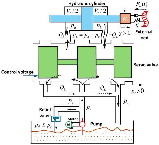
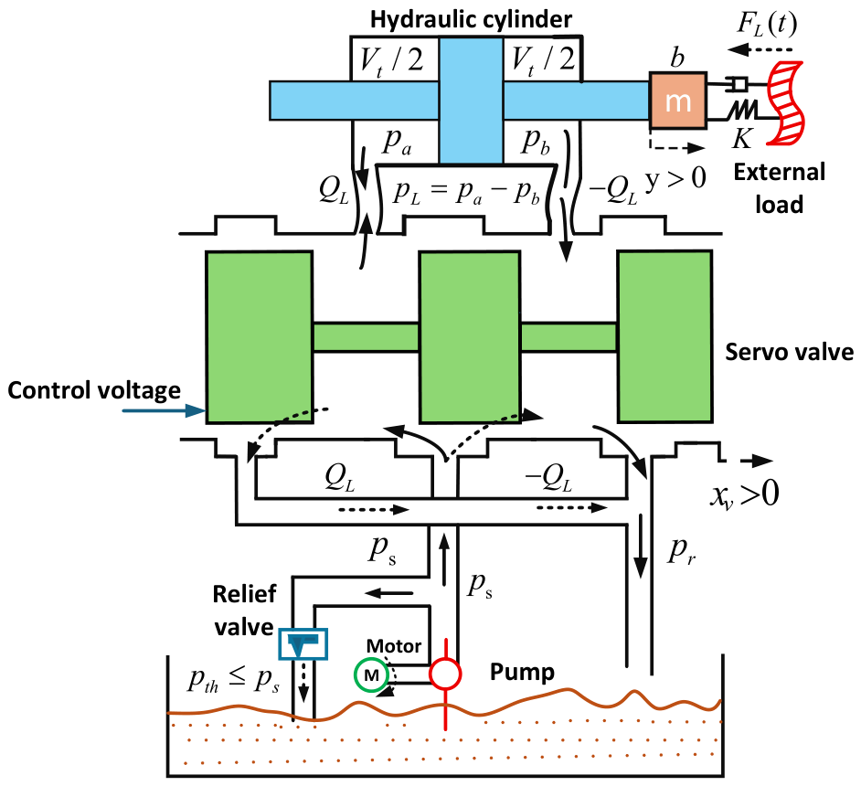
The hydraulic cylinder is the core actuator of the EHSs, which can convert hydraulic energy into precise linear mechanical motion. Its schematic diagram is shown in Figure 1: the voltage control signal applied to the servo valve affects the spool displacement and ultimately determines the actual output of the hydraulic cylinder. Due to the different directions and magnitudes of the voltage control signal, the spool displacement of the servo valve exhibits three states. When $x_v>0$, the left chamber is connected to the forward passage. Hydraulic oil is injected into the left chamber through the servo valve, driving the hydraulic cylinder forward, while oil from the right chamber flows out via the return passage; When $x_v<0$, the right chamber is switched to the forward channel; hydraulic oil flows into the right chamber, and the oil in the left chamber is discharged through the return channel.

Figure 1. The electro-hydraulic system mechanism: $P_a$ and $P_b$ are the channel’s pressures; $P_r$ is the return pressure; $P_{th}$ is the pressure threshold of the relief valve, u is the control voltage of servo valve.

For EHSs subject to an input time delay $\tau$, the servo valve spool position $x_v$ exhibits a linear dependence on the control voltage u, as expressed below

$$\begin{array}{c}\hfill x_v=K_{sv}u(t-\tau )\end{array}$$

(1)

where $K_{sv}$ is the control gain. According to relevant literature on hydraulic transmission and control, the specific form of the flow-pressure characteristic equation for electro-hydraulic servo valves is as

$$\begin{array}{c}\hfill Q_L={\displaystyle \frac{1}{\sqrt{\rho }}}{C}_{d}w{x}_v\sqrt{p_s-\mathrm{sign}\left(x_v\right)p_L}\end{array}$$

(2)

where $Q_L$ denotes the load flow; w is the area gradient; $\rho$ represents the hydraulic oil density; $C_d$ stands for the flow coefficient of the orifice in the EHSs; $p_s$ indicates the supply pressure; and $\mathrm{sign}(·)$ denotes the signum function, defined as $\mathrm{sign}\left(x\right)=1$ for $x>0$, $\mathrm{sign}\left(x\right)=-1$ for $x<0$, and $\mathrm{sign}\left(x\right)=0$ otherwise. Additionally, a continuous examination of the flow-pressure relationship within hydraulic actuators is conducted.

$$\begin{array}{c}\hfill Q_L=A_p\dot{y}+{\displaystyle \frac{1}{4}}{V}_t{\dot{p}}_L{\beta }_e+C_{tl}{p}_L\end{array}$$

(3)

where $A_p$ is the effective piston area, $C_{tl}$ is the leakage coefficient, $V_t$ is the total fluid volume of the hydraulic system and ${\beta }_e$ is the elastic coefficient of the hydraulic fluid.

According to Newton’s second law of motion, the mechanical equilibrium equation for the dynamic structure is as follows

$$\begin{array}{c}\hfill m\ddot{y}=-Ky-b\dot{y}+p_L{A}_p-F_L\left(t\right)\end{array}$$

(4)

where K is the load spring stiffness, b is the viscous damping coefficient, m is the load mass, and $F_L$ is the unknown external load disturbance.

Based on the foregoing three dynamic formulas, the third-order nonlinear state-space EHSs mathematical model with input delay $\tau$ can be established as

$$\left\{\begin{array}{cc}\hfill {\dot{x}}_1& =x_2\hfill \\ \hfill {\dot{x}}_2& ={\displaystyle \frac{1}{m}}\left(x_3-K{x}_1-b{x}_2-F_L\left(t\right)\right)\hfill \\ \hfill {\dot{x}}_3& =-{\displaystyle \frac{4{\beta }_e{A}_p^2}{V_t}}{x}_2-{\displaystyle \frac{4{\beta }_e{C}_{tl}}{V_t}}{x}_3+{\displaystyle \frac{4{\beta }_e{C}_{d}w{K}_{sv}{A}_p}{V_t\sqrt{\rho }}}\sqrt{p_s-\mathrm{sign}\left(u\right)x_3/A_p}u(t-\tau )\hfill \\ \hfill y& =x_1\hfill \end{array}\right.$$

(5)

where ${[x_1,x_2,x_3]}^{\mathrm{T}}={[y,\dot{y},A_p{p}_L]}^{\mathrm{T}}$; y is the displacement output, $\dot{y}$ is its velocity and $A_p{p}_L$ is the hydraulic pressure supplied to the actuator. The control signal u is input to the model and the displacement output y is the system state output.

When considering small input delay for EHSs, conventional backstepping control approach is unable to effectively overcome the negative effects caused by control lag. Therefore, this paper mathematically processes the delay system model via Laplace transform together with Padé approximation.

At first, according to the Laplace transform, it holds that

$$L\left[u(t-\tau )\right]=e^{-\tau s}L\left[u\left(t\right)\right]={\displaystyle \frac{e^{-\tau s/2}}{e^{\tau s/2}}}L\left[u\left(t\right)\right]$$

(6)

where $L[•]$ denotes the Laplace transform, and s denotes the Laplace operator. This transformation operation converts the delay term $\tau$ into an external parameter.

Since the delay $\tau$ in this paper is considered as a small value, the $e^{-\tau s}$ can be approximated as ${\displaystyle \frac{1-\tau s/2}{1+\tau s/2}}$ by means of Padé approximation, and thus

$${\displaystyle \frac{e^{-\tau s/2}}{e^{\tau s/2}}}L\left[u\left(t\right)\right]\approx {\displaystyle \frac{1-\tau s/2}{1+\tau s/2}}L\left[u\left(t\right)\right]$$

(7)

Here, define the intermediate variable $x_4$ to satisfy the Laplace transform

$$L\left[x_4\left(t\right)\right]-L\left[u\left(t\right)\right]={\displaystyle \frac{1-\tau s/2}{1+\tau s/2}}L\left[u\left(t\right)\right]$$

(8)

Rearranging the above equation yields

$$2L\left[x_4\left(t\right)\right]=4L\left[u\left(t\right)\right]-\tau sL\left[x_4\left(t\right)\right]$$

(9)

Performing the inverse Laplace transform on the above formula gets

$${\dot{x}}_4\left(t\right)={\displaystyle \frac{4}{\tau }}u\left(t\right)-{\displaystyle \frac{2}{\tau }}{x}_4\left(t\right)$$

(10)

Introducing the variable $\gamma ={\displaystyle \frac{2}{\tau }}$, one gets

$${\dot{x}}_4=2\gamma u-\gamma x_4$$

(11)

Summarizing all the above equations yields a fourth-order EHSs (F-EHSs) dynamic model incorporating input delay

$$\left\{\begin{array}{cc}\hfill {\dot{x}}_1& =x_2,\hfill \\ \hfill {\dot{x}}_2& ={\overline{g}}_2{x}_3+{\overline{f}}_2(x_1,x_2)-F_L/m+{\mathrm{\Theta }}_2(\tilde{k},\tilde{b},x_1,x_2)\hfill \\ \hfill {\dot{x}}_3& ={\overline{g}}_3{x}_4-{\overline{g}}_{3}u+{\overline{f}}_3+{\mathrm{\Theta }}_3(\tilde{\omega },{\tilde{c}}_{tl},{\tilde{\beta }}_e,{\tilde{c}}_d,\tilde{\rho },u,x)\hfill \\ \hfill {\dot{x}}_4& =-\gamma x_4+2\gamma u\hfill \\ \hfill y& =x_1\hfill \end{array}\right.$$

(12)

where the known nominal model is presented as follows

$$\left\{\begin{array}{cc}\hfill {\overline{g}}_2& ={\displaystyle \frac{1}{m}}\hfill \\ \hfill {\overline{f}}_2& =-{\displaystyle \frac{\overline{K}{x}_1+\overline{b}{x}_2}{m}}\hfill \\ \hfill {\overline{g}}_3& ={\displaystyle \frac{4{\overline{\beta }}_e{\overline{C}}_d\overline{w}{K}_{sv}{A}_p}{V_t\sqrt{\overline{\rho }}}}\sqrt{p_s-\mathrm{sign}\left(u\left(t\right)\right)x_3/A_p}\hfill \\ \hfill {\overline{f}}_3& =-{\displaystyle \frac{4{\overline{\beta }}_e{A}_p^2}{V_t}}{x}_2-{\displaystyle \frac{4{\overline{\beta }}_e{\overline{C}}_{tl}}{V_t}}{x}_3\hfill \end{array}\right.$$

(13)

The uncertainty arising from model mismatch can be expressed as

$${\mathrm{\Theta }}_2(·)=-{\displaystyle \frac{\tilde{K}{x}_1+\tilde{b}{x}_2}{m}}$$

(14)

Meanwhile, the mismatched uncertainty is given by

$${\mathrm{\Theta }}_3(·)={\tilde{\phi }}_3(\tilde{\omega },{\tilde{c}}_{tl},{\tilde{\beta }}_e,{\tilde{c}}_d,\tilde{\rho },u,x)+{\tilde{f}}_3({\tilde{\beta }}_e,{\tilde{C}}_{tl},x)$$

(15)

where $x=[x_1,x_2,x_3]$ is the vector of system state, and $\widetilde{{\phi }_3}$ and $\widetilde{f_3}$ are uncertain terms caused by uncertain hydraulic parameters.

Assumption 1 

([40]). The desired displacement $y_d$ and the corresponding multiple order derivative ${\dot{y}}_d$, ${\ddot{y}}_d$ possess smoothness and boundedness.

Assumption 2 

([41]). The uncertain parameters ${\mathrm{\Theta }}_2$, ${\mathrm{\Theta }}_3$ and the load disturbance signal $F_L$ are both continuous and bounded.

Remark 1.

EHSs includes time-varying parametric uncertainties such as oil bulk modulus, internal leakage, viscous friction and load stiffness. These uncertainties result in model mismatch, reduce tracking accuracy and cause steady-state errors, aggravate nonlinear coupling and weaken the anti-disturbance performance of the controller, and may lead to system oscillation and instability in severe cases.

2.2. Preliminaries

Lemma 1 

([42]). For a nonlinear system described by $\dot{y}=f\left(y\right)$ with state vector $y\in {\mathbb{R}}^n$, initial condition $y\left(0\right)=y_0$, and $f\left(0\right)=0$, the existence of a continuous and positive-definite function $V\left(z\right)$ over a domain U ensures that

$$\dot{V}\left(z\right)\le -\alpha V\left(z\right)-\beta V^{\gamma }\left(z\right)+\xi ,z\in U\setminus \left\{0\right\}$$

(16)

where $\alpha \in (0,\infty )$, $\beta \in (0,\infty )$, $\gamma \in (0,1)$, $\xi \in (0,\infty )$, Under these conditions, system achieves practical fast finite-time stability. Hence, its solution set can be described as follows

$$\Delta =\left\{z|V\left(z\right)\le min\left\{{\displaystyle \frac{\xi }{(1-\theta )\alpha }},{\left({\displaystyle \frac{\xi }{(1-\theta )\beta }}\right)}^{{\displaystyle \frac{1}{\gamma }}}\right\}\right\}$$

(17)

where θ is a scalar satisfying $\theta \in (0,1)$, and $T\left(z\right)$ is defined as the upper bound of the convergence time for the system states to converge to the steady-state bounded neighborhood from the initial state z, can be obtained according to the initial state information and satisfies the inequality as follows

$$T\left(z\right)\le {\displaystyle \frac{1}{\alpha (1-\gamma )}}ln{\displaystyle \frac{\alpha V^{1-\gamma }\left(z\right)+\beta }{\beta }}$$

(18)

Lemma 2 

([43]). For arbitrary constants $x_1>x_2$ and $q>1$, one has

$$x_2{(x_1-x_2)}^q\le (x_1^{q+1}-x_2^{q+1}){\displaystyle \frac{q}{q+1}}$$

(19)

where the equality holds if and only if $x_1=x_2$.

Lemma 3

(Young’s Inequality). For any $a\in \mathbb{R}$, $c\in \mathbb{R}$, $r>1$, $q>1$ with ${\displaystyle \frac{1}{q}}+{\displaystyle \frac{1}{r}}=1$, the inequality given below is obtained

$$ac\le {\displaystyle \frac{1}{q}}{\left|a\right|}^q+{\displaystyle \frac{1}{r}}{\left|c\right|}^r$$

(20)

where the equality holds if and only if ${\left|a\right|}^q={\left|c\right|}^r$.

Lemma 4

(reverse Young’s inequality [44]). Suppose $0<p<1$, $q<0$ and ${\displaystyle \frac{1}{p}}+{\displaystyle \frac{1}{q}}=1$. For $\tau >0$ and non-negative real numbers $a,b$, the inequality reverses

$$ab\ge {\displaystyle \frac{{\tau }^p{a}^p}{p}}+{\displaystyle \frac{b^q}{q{\tau }^q}}$$

(21)

where the equality holds if and only if ${\tau }^p{a}^p=b^q$.

Lemma 5 

([45]). For arbitrary constants $c_i>0$, $0<{\hslash }_1\le 1$, and ${\hslash }_2>1$, one has

$${\left(\sum _{i=1}^n{c}_i\right)}^{{\hslash }_1}\le \sum _{i=1}^n{c}_i^{{\hslash }_1}$$

(22)

$${\left(\sum _{i=1}^n{c}_i\right)}^{{\hslash }_2}\le n^{{\hslash }_2-1}\sum _{i=1}^n{c}_i^{{\hslash }_2}$$

(23)

2.3. The Approximation Theory of Neural Networks

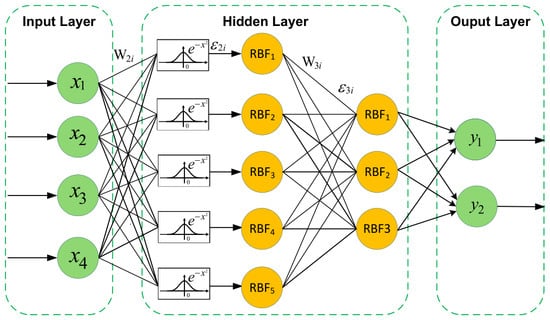
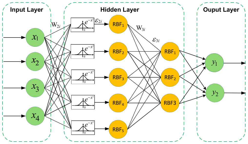
The RBFNNs neural network is a feedforward network. The input layer receives raw data and uses it as the initial activation value; the intermediate multi-layer hidden layers extract features from the data layer by layer through the weighted summation of n neurons and the operation of the activation function. The final output layer further operates on the processing results of the hidden layers, completes the analysis and response to the input data, and can be applied to various tasks such as classification and regression. The corresponding schematic diagram is shown in Figure 2. Among them, the connection weight between the input layer and the hidden layer is $C_i$, the threshold value of the hidden layer is ${\displaystyle \frac{1}{h_i}}$. The output of the ith neuron in hidden layer is

$${\mathcal{G}}_i\left(\mathcal{X}\right)=exp\left[-{\displaystyle \frac{{(\mathcal{X}-{\mathcal{C}}_i)}^T(\mathcal{X}-{\mathcal{C}}_i)}{h_i^2}}\right]$$

(24)

Figure 2. Schematic diagram of RBFNNs.

According to the local approximation property of RBFNNs, a continuous function $\Delta \left(\mathcal{X}\right)\to \mathbb{R}$ defined on a compact set can be approximated as [46]

$$\Delta \left(\mathcal{X}\right)=W^{\ast \mathrm{T}}\mathcal{G}\left(\mathcal{X}\right)+\mathcal{E}\left(\mathcal{X}\right)$$

(25)

where $\mathcal{X}={[{\mathcal{X}}_1,{\mathcal{X}}_2,\dots ,{\mathcal{X}}_p]}^{\mathrm{T}}\in {\mathrm{\Omega }}_{\mathcal{X}}$ is the input vector; $\Delta \left(\mathcal{X}\right)$ is the basis function vector; $\mathcal{G}\left(\mathcal{X}\right)={[{\mathcal{G}}_1\left(\mathcal{X}\right),{\mathcal{G}}_2\left(\mathcal{X}\right),\dots ,{\mathcal{G}}_N\left(\mathcal{X}\right)]}^{\mathrm{T}}$ is the basis function vector with N, the neuron number. The approximation error $\mathcal{E}\left(\mathcal{X}\right)$ satisfies the boundedness condition $\parallel \mathcal{E}\left(\mathcal{X}\right)\parallel \le \overline{\mathcal{E}}$, where $\overline{\mathcal{E}}>0$ is a positive constant. The unknown ideal weight vector is defined as follows

$$W*\triangleq arg\underset{W\in {\mathbb{R}}^N}{min}\left\{\underset{\mathcal{X}\in {\mathrm{\Omega }}_{\mathcal{X}}}{sup}\left|\Delta \left(\mathcal{X}\right)-W^{\mathrm{T}}\mathcal{G}\left(\mathcal{X}\right)\right|\right\}$$

(26)

for some ideal weights $W_i^{*}$, with $\Delta \left(\mathcal{X}\right)$ and $\mathcal{E}\left(\mathcal{X}\right)$ respectively as a nonlinear activation function and functional reconstruction accuracy, the model enables high-precision feedforward compensation of model uncertainties.

3. Neural Adaptive Finite-Time Controller Design

In this section, a neural adaptive backstepping controller will be designed, which can guarantee that the system states converge to the equilibrium point in finite time.

3.1. Controller Design

The controller designed in this paper will adopt the traditional backstepping method since the EHSs exhibit significant nonlinear characteristics. The RBFNNs are also considered because their outstanding ability to estimate the unknown nonlinearities of the system. To facilitate controller design, the state errors are defined as follows

$$\left\{\begin{array}{cc}\hfill z_1& =x_1-x_d\hfill \\ \hfill z_2& =x_2-{\alpha }_2\hfill \\ \hfill z_3& =x_3-{\alpha }_3+{\displaystyle \frac{g_3}{\gamma }}{x}_4\hfill \end{array}\right.$$

(27)

where ${\alpha }_2$ and ${\alpha }_3$ are virtual control variables and $x_d$ is the desired trajectory. Furthermore, (27) can be differentiated as

$$\left\{\begin{array}{cc}\hfill {\dot{z}}_1& ={\dot{x}}_1-{\dot{x}}_d\hfill \\ \hfill {\dot{z}}_2& ={\overline{g}}_2{x}_3+{\overline{f}}_2-{\displaystyle \frac{F_L}{m}}+{\mathrm{\Theta }}_2-{\alpha }_2-{\dot{\alpha }}_2\hfill \\ \hfill {\dot{z}}_3& ={\overline{f}}_3+{\overline{g}}_{3}u\left(t\right)+{\mathrm{\Theta }}_3-{\alpha }_3-{\dot{\alpha }}_3\hfill \end{array}\right.$$

(28)

Define the candidate Lyapunov function $V_1$ as

$$V_1={\displaystyle \frac{1}{2}}{z}_1^2$$

(29)

Combining (27) and (28) and differentiating $V_1$, it yields that

$${\dot{V}}_1=z_1{\dot{z}}_1=z_1(z_2+{\alpha }_2-{\dot{x}}_d)$$

(30)

Design ${\alpha }_2$ as

$${\alpha }_2=-k_1{z}_1-b_1{z}_1^{2h-1}+{\dot{x}}_d$$

(31)

where ${\displaystyle \frac{1}{2}}<h<1$, $k_1>0$ and $b_1>0$ are adjustable control parameters. Then, (30) can be rewritten as

$${\dot{V}}_1=-k_1{z}_1^2-b_1{z}_1^{2h}+z_1{z}_2$$

(32)

Define the candidate Lyapunov function $V_2$ as

$$V_2={\displaystyle \frac{1}{2}}{z}_2^2$$

(33)

Combining (27) and (28) and differentiating $V_2$, it yields that

$$\begin{array}{cc}\hfill {\dot{V}}_2& =z_2{\dot{z}}_2\hfill \\ \hfill & =z_2\left({\overline{g}}_2{x}_3+{\overline{f}}_2-{\displaystyle \frac{F_L}{m}}+{\Delta }_2\left({\mathcal{X}}_2\right)\right)\hfill \\ \hfill & =z_2\left({\overline{g}}_2{z}_3+{\overline{g}}_2{\alpha }_3-{\displaystyle \frac{{\overline{g}}_2{\overline{g}}_3}{\gamma }}{x}_4+{\overline{f}}_2+{\displaystyle \frac{F_L}{m}}+{\Delta }_2\left({\mathcal{X}}_2\right)\right)\hfill \end{array}$$

(34)

where ${\Delta }_2\left({\mathcal{X}}_2\right)={\mathrm{\Theta }}_2-{\alpha }_2$ is defined as a lumped uncertain term, with ${\mathcal{X}}_2={\left[x_1,x_2,y_d,{\dot{y}}_d,{\ddot{y}}_d\right]}^{\mathrm{T}}$. Moreover, through the RBFNNs approximation strategy, one gets

$${\Delta }_2\left({\mathcal{X}}_2\right)=W_2^{\ast \mathrm{T}}{\mathcal{G}}_2\left({\mathcal{X}}_2\right)+{\mathcal{E}}_2\left({\mathcal{X}}_2\right)$$

(35)

where $\left|{\mathcal{E}}_2\left({\mathcal{X}}_2\right)\right|\le {\overline{\mathcal{E}}}_2$ with ${\overline{\mathcal{E}}}_2>0$.

According to Lemmas 3 and 4, the following inequality holds

$$\begin{array}{cc}\hfill z_2{\Delta }_2\left({\mathcal{X}}_2\right)=& z_2{\vartheta }_2{\mathcal{G}}_2\left({\mathcal{X}}_2\right)+z_2{\mathcal{E}}_2\left({\mathcal{X}}_2\right)\hfill \\ \hfill \le & {\displaystyle \frac{1}{2{\tau }_2}}{z}_2^2{\vartheta }_2{∥{\mathcal{G}}_2\left({\mathcal{X}}_2\right)∥}^2+{\displaystyle \frac{{\tau }_2}{2}}+{\displaystyle \frac{1}{2}}{z}_2^2+{\displaystyle \frac{1}{2}}{\overline{\mathcal{E}}}_2^2\hfill \\ \hfill -z_2{\displaystyle \frac{F_L}{m}}\le & {\displaystyle \frac{1}{2}}{z}_2^2+{\displaystyle \frac{1}{2}}{\overline{F}}_L^2\hfill \end{array}$$

(36)

where ${\overline{F}}_L$ denotes the upper bound of ${\displaystyle \frac{F_L}{m}}$, ${\tau }_2>0$, ${\vartheta }_2={∥W_2^{*}∥}^2$, ${\mathcal{X}}_2={\left[x_1,x_2,y_d,{\dot{y}}_d,{\ddot{y}}_d\right]}^{\mathrm{T}}$.

To make (34) negative definite, the virtual controller ${\alpha }_3$ is designed as

$${\alpha }_3={\displaystyle \frac{1}{{\overline{\phi }}_2}}\left(-k_2{z}_2-b_2{z}_2^{2h}-{\displaystyle \frac{1}{2{\tau }_2}}{z}_2{\widehat{\vartheta }}_2{\parallel {\mathcal{G}}_2\left({\mathcal{X}}_2\right)\parallel }^2-z_1-{\displaystyle \frac{3}{2}}{z}_2-{\overline{f}}_2\right)$$

(37)

where $k_2,b_2>0$ are design parameters, ${\widehat{\vartheta }}_2$ is the estimate of ${\vartheta }_2$, and ${\tilde{\vartheta }}_2\triangleq {\vartheta }_2-{\widehat{\vartheta }}_2$ is the estimation error. Substituting (35)–(37) into (34), it can be obtained that

$$\begin{array}{cc}\hfill {\dot{V}}_2& \le -g_2{z}_2{z}_3-z_1{z}_2-k_2{z}_2^2-b_2{z}_2^{2h}+{\displaystyle \frac{{\tau }_2}{2}}+{\displaystyle \frac{1}{2}}{\overline{\mathcal{E}}}_2^2\hfill \\ \hfill & +{\displaystyle \frac{1}{2{\tau }_2}}{z}_2^2{\tilde{\vartheta }}_2{\parallel {\mathcal{G}}_2\left({\mathcal{X}}_2\right)\parallel }^2+{\displaystyle \frac{1}{2}}{\left({\displaystyle \frac{{\overline{g}}_2{\overline{g}}_3}{\gamma }}{x}_4\right)}^2+{\displaystyle \frac{1}{2}}{\overline{F}}_L^2\hfill \end{array}$$

(38)

Define the candidate Lyapunov function $V_3$ as

$$V_3={\displaystyle \frac{1}{2}}{z}_3^2$$

(39)

Similarly to the above operations, it follows that

$${\dot{V}}_3=z_3\left({\overline{g}}_{3}u+{\overline{f}}_3+{\Delta }_3\left({\mathcal{X}}_3\right)\right)$$

(40)

where ${\Delta }_3\left({\mathcal{X}}_3\right)={\mathrm{\Theta }}_3-{\dot{\alpha }}_3$ is also an uncertain packing function with ${\mathcal{X}}_3={\left[x_1,x_2,x_3,y_d,{\dot{y}}_d,{\ddot{y}}_d\right]}^{\mathrm{T}}$. The approximating of ${\Delta }_3\left({\mathcal{X}}_3\right)$ follows that

$${\Delta }_3\left({\mathcal{X}}_3\right)=W_3^{\ast \mathrm{T}}{\mathcal{G}}_3\left({\mathcal{X}}_3\right)+{\mathcal{E}}_3\left({\mathcal{X}}_3\right)$$

(41)

where $\left|{\mathcal{E}}_3\left({\mathcal{X}}_3\right)\right|\le {\overline{\mathcal{E}}}_3$ with ${\overline{\mathcal{E}}}_3>0$. And the following inequality also hold according to Lemma 4 as

$$\begin{array}{cc}\hfill z_3{\Delta }_3\left({\mathcal{X}}_3\right)& =z_3{\vartheta }_3{\mathcal{G}}_3\left({\mathcal{X}}_3\right)+z_3{\mathcal{E}}_3\left({\mathcal{X}}_3\right)\hfill \\ \hfill & \le {\displaystyle \frac{1}{2{\tau }_3}}{z}_3^2{\vartheta }_3{∥{\mathcal{G}}_3\left({\mathcal{X}}_3\right)∥}^2+{\displaystyle \frac{{\tau }_3}{2}}+{\displaystyle \frac{1}{2}}{z}_3^2+{\displaystyle \frac{1}{2}}{\overline{\mathcal{E}}}_3^2\hfill \end{array}$$

(42)

where ${\overline{F}}_L$ is the upper bound of ${\displaystyle \frac{F_L}{m}}$, ${\tau }_3>0$, ${\vartheta }_3={∥W_3^{*}∥}^2$, ${\mathcal{X}}_2={\left[x_1,x_2,y_d,{\dot{y}}_d,{\ddot{y}}_d\right]}^{\mathrm{T}}$.

Ultimately, the final control input signal u is designed as

$$u={\displaystyle \frac{1}{{\overline{g}}_3}}\left(-k_3{z}_3-b_3{z}_3^{2h-1}-{\displaystyle \frac{1}{2{\tau }_3}}{z}_3{\widehat{\vartheta }}_3{\parallel {\mathcal{G}}_3\left({\mathcal{X}}_3\right)\parallel }^2-{\displaystyle \frac{z_3}{2}}-{\overline{g}}_2{z}_2-{\overline{f}}_3\right)$$

(43)

where $k_3,b_3>0$ are design parameters, ${\widehat{\vartheta }}_3$ is the estimate of ${\vartheta }_3$, and ${\tilde{\vartheta }}_3\triangleq {\vartheta }_3-{\widehat{\vartheta }}_3$ is the estimation error. Combining (40)–(43) yields

$$\begin{array}{cc}\hfill {\dot{V}}_3& \le -{\overline{g}}_2{z}_2{z}_3-k_3{z}_3^2-b_3{z}_3^{2h}+{\displaystyle \frac{{\tau }_3}{2}}+{\displaystyle \frac{1}{2}}{\overline{\mathcal{E}}}_3^2+{\displaystyle \frac{1}{2{\tau }_3}}{z}_3^2{\tilde{\vartheta }}_3{\parallel {\mathcal{G}}_3\left({\mathcal{X}}_3\right)\parallel }^2+{\displaystyle \frac{1}{2}}{\left({\displaystyle \frac{{\overline{g}}_2{\overline{g}}_3}{\gamma }}{x}_4\right)}^2\hfill \end{array}$$

(44)

To ensure the finite-time convergence of ${\tilde{\vartheta }}_i$ ($i=2,3$), the adaptive estimation law, the adaptive estimation laws designed as follows

$${\dot{\widehat{\vartheta }}}_i={\displaystyle \frac{r_i{z}_i^2{\parallel {\mathcal{G}}_i\left({\mathcal{X}}_i\right)\parallel }^2}{2{\tau }_i}}-{\xi }_i{\widehat{\vartheta }}_i-{\sigma }_i{\widehat{\vartheta }}_i^{2h-1},i\in \{2,3\}$$

(45)

where $r_i,{\xi }_i,{\sigma }_i>0$.

Remark 2.

Backstepping control eliminates nonlinear terms layer by layer via recursive design to solve control difficulties of high-order nonlinear systems; adaptive control identifies parameters online and corrects control laws dynamically to effectively suppress system uncertainties and external disturbances. The combination of the two reduces dependence on modeling accuracy and adapts to time-varying operating conditions, which enhances the stability and robustness of the system.

3.2. Stability Analysis

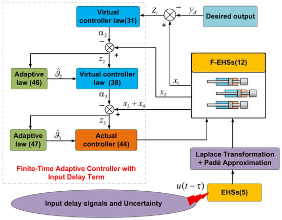
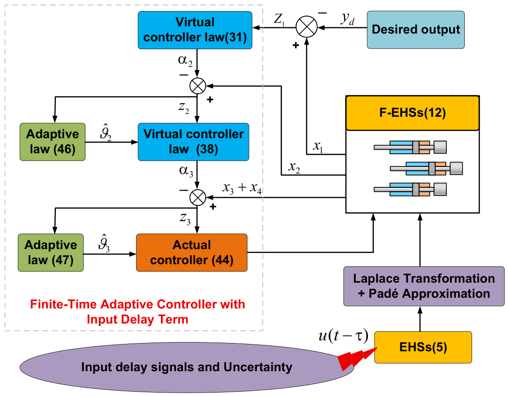
In this section, stability analysis is provided for the nonlinear system with model uncertainty and input delay described in (12). Figure 3 illustrates the proposed FTANC scheme, which consists of the actual controller (43) virtual controllers (31), (37) and adaptive laws (45).

Figure 3. The block diagram of the proposed FTANC scheme.

Theorem 1.

Considering the F-EHSs model (12), together with the designed control variables in (31), (37) and (43), the fast finite-time stability of the F-EHSs is achieved, and it follows that

• All error signals $z_1$, $z_2$, $z_3$, ${\tilde{\vartheta }}_2$ and ${\tilde{\vartheta }}_3$ converge to a neighborhood of zero within a finite time.
• All signals in the closed-loop system $x_1$, $x_2$, $x_3$, ${\alpha }_1$, ${\alpha }_2$, ${\widehat{\vartheta }}_2$, ${\widehat{\vartheta }}_3$ and u stay bounded.

Proof. 

To ensure all designed signals are bounded, Lyapunov function is constructed as follows

$$V=V_1+V_2+V_3+{\displaystyle \frac{1}{2}}\sum _{i=2}^3{\displaystyle \frac{1}{r_i}}{\tilde{\vartheta }}_i^2$$

(46)

Differentiating (46) yields

$$\dot{V}={\dot{V}}_1+{\dot{V}}_2+{\dot{V}}_3-\sum _{i=2}^3{\displaystyle \frac{1}{r_i}}{\tilde{\vartheta }}_i{\dot{\widehat{\vartheta }}}_i$$

(47)

Substituting (32), (38), (44) into (47) gives

$$\begin{array}{cc}\hfill \dot{V}\le & -\sum _{i=1}^3{k}_i{z}_i^{2h}-\sum _{i=1}^3{b}_i{z}_i^{2l}+\sum _{i=2}^3\left({\displaystyle \frac{{\tau }_i}{2}}+{\displaystyle \frac{1}{2}}{\overline{\mathcal{E}}}_i^2\right)\hfill \\ \hfill & +\sum _{i=2}^3{\displaystyle \frac{1}{r_i}}{\xi }_i{\tilde{\vartheta }}_i{\widehat{\vartheta }}_i+\sum _{i=2}^3{\displaystyle \frac{1}{r_i}}{\sigma }_i{\tilde{\vartheta }}_i{\widehat{\vartheta }}_i^{2l-1}+{\displaystyle \frac{1}{2}}{\overline{F}}_L^2+{\displaystyle \frac{1}{2}}{\left({\displaystyle \frac{{\overline{g}}_2{\overline{g}}_3}{\gamma }}{x}_4\right)}^2\hfill \end{array}$$

(48)

From Lemma 2, one has

$${\displaystyle \frac{1}{r_i}}{\sigma }_i{\tilde{\vartheta }}_i{\widehat{\vartheta }}_i^{2h-1}\le ({\vartheta }_i^{2h}-{\tilde{\vartheta }}_i^{2h}){\displaystyle \frac{2h-1}{2h{r}_i}}{\sigma }_i$$

(49)

Thus, one has

$$\begin{array}{cc}\hfill \dot{V}\le & -\sum _{i=1}^3{k}_i{z}_i^2-\sum _{i=1}^3{b}_i{z}_i^{2h}+\sum _{i=2}^3\left({\displaystyle \frac{1}{2{\tau }_i}}+{\displaystyle \frac{1}{2}}{\overline{\mathcal{E}}}_i^2\right)-\sum _{i=2}^3{\displaystyle \frac{1}{r_i}}{\sigma }_i{\tilde{\vartheta }}_i{\widehat{\vartheta }}_i^{2h-1}\hfill \\ \hfill & +\sum _{i=2}^3{\displaystyle \frac{2h-1}{2h{r}_i}}{\sigma }_i{\vartheta }_i^{2h}-\sum _{i=2}^3{\displaystyle \frac{2h-1}{2h{r}_i}}{\sigma }_i{\tilde{\vartheta }}_i^{2h}+{\displaystyle \frac{1}{2}}{\overline{F}}_L^2+{\displaystyle \frac{1}{2}}{\left({\displaystyle \frac{{\overline{g}}_2{\overline{g}}_3}{\gamma }}{x}_4\right)}^2\hfill \end{array}$$

(50)

According to Lemma 3, one gets

$$\begin{array}{cc}\hfill {\displaystyle \frac{1}{r_i}}{\xi }_i{\tilde{\vartheta }}_i{\widehat{\vartheta }}_i& ={\displaystyle \frac{1}{r_i}}{\xi }_i{\tilde{\vartheta }}_i{\vartheta }_i-{\displaystyle \frac{1}{r_i}}{\xi }_i{\tilde{\vartheta }}_i^2\hfill \\ \hfill & \le {\displaystyle \frac{1}{2r_i}}{\xi }_i{\tilde{\vartheta }}_i^2+{\displaystyle \frac{1}{2r_i}}{\xi }_i{\vartheta }_i^2-{\displaystyle \frac{1}{r_i}}{\xi }_i{\tilde{\vartheta }}_i^2\hfill \\ \hfill & \le -{\displaystyle \frac{1}{2r_i}}{\xi }_i{\tilde{\vartheta }}_i^2+{\displaystyle \frac{1}{2r_i}}{\xi }_i{\vartheta }_i^2\hfill \end{array}$$

(51)

Combining (50) and (51) yields

$$\begin{array}{cc}\hfill \dot{V}& \le -\sum _{i=1}^3{k}_i{z}_i^2-\sum _{i=1}^3{b}_i{z}_i^{2h}-\sum _{i=2}^3{\displaystyle \frac{1}{2r_i}}{\xi }_i{\tilde{\vartheta }}_i^2-\sum _{i=2}^3{\displaystyle \frac{2h-1}{2h{r}_i}}{\sigma }_i{\tilde{\vartheta }}_i^{2h}+\Gamma \hfill \end{array}$$

(52)

where

$$\begin{array}{cc}\hfill \Gamma & =\sum _{i=2}^3\left({\displaystyle \frac{{\tau }_i}{2}}+{\displaystyle \frac{1}{2}}{\overline{\mathcal{E}}}_i^2\right)+\sum _{i=2}^3{\displaystyle \frac{2h-1}{2h{r}_i}}{\sigma }_i{\vartheta }_i^{2h}+\sum _{i=2}^3{\displaystyle \frac{1}{2r_i}}{\xi }_i{\vartheta }_i^2+{\displaystyle \frac{1}{2}}{\overline{F}}_L^2+{\displaystyle \frac{1}{2}}{\left({\displaystyle \frac{{\overline{g}}_2{\overline{g}}_3}{\gamma }}{x}_4\right)}^2\hfill \end{array}$$

(53)

Using Lemma 5 to relax (53) yields

$$\begin{array}{cc}\hfill \dot{V}=& -2k_i\left({\displaystyle \frac{1}{2}}\sum _{i=1}^3{z}_i^2\right)-2^h{b}_i{\left({\displaystyle \frac{1}{2}}\sum _{i=1}^3{z}_i^2\right)}^h-{\xi }_i\left({\displaystyle \frac{1}{2}}\sum _{i=2}^3{\displaystyle \frac{1}{r_i}}{\tilde{\vartheta }}_i^2\right)\hfill \\ \hfill & -2^{h-1}{\displaystyle \frac{2h-1}{h}}{\sigma }_i{r}_i^{h-1}{\left({\displaystyle \frac{1}{2}}\sum _{i=2}^3{\displaystyle \frac{1}{r_i}}{\tilde{\vartheta }}_i^2\right)}^h+\Gamma \hfill \\ \hfill \le & -{\omega }_1\left({\displaystyle \frac{1}{2}}\sum _{i=1}^3{z}_i^2\right)-{\varphi }_1{\left({\displaystyle \frac{1}{2}}\sum _{i=1}^3{z}_i^2\right)}^h-{\omega }_2\left({\displaystyle \frac{1}{2}}\sum _{i=2}^3{\displaystyle \frac{1}{r_i}}{\tilde{\vartheta }}_i^2\right)\hfill \\ \hfill & -{\varphi }_2{\left({\displaystyle \frac{1}{2}}\sum _{i=2}^3{\displaystyle \frac{1}{r_i}}{\tilde{\vartheta }}_i^2\right)}^h+\Gamma \hfill \end{array}$$

(54)

where ${\omega }_1=2min\{k_1,k_2,k_3\}$, ${\varphi }_1=2^{h}min\{b_1,b_2,b_3\}$, ${\varphi }_2=2^{h-1}{\displaystyle \frac{2^h-1}{h}}min\{r_2^{h-1}{\sigma }_2,r_3^{h-1}{\sigma }_3\}$, ${\omega }_2=min\{{\xi }_2,{\xi }_3\}$.

Finally, one gets

$$\dot{V}\le -\omega V-\varphi V^h+\Gamma$$

(55)

where $\omega =min\{{\omega }_1,{\omega }_2\}$ and $\varphi =2^{1-h}min\{{\varphi }_1,{\varphi }_2\}$ and $\omega \in (0,\infty )$, $\varphi \in (0,\infty )$. Based on Lemma 1, the error signals are ultimately converge to the region

$$\Delta =\left\{z|V\left(z\right)\le min\left\{{\displaystyle \frac{\Gamma }{(1-\theta )\omega }},{\left({\displaystyle \frac{\Gamma }{(1-\theta )\varphi }}\right)}^{{\displaystyle \frac{1}{h}}}\right\}\right\}$$

(56)

where $\Delta ={[z_1,z_2,z_3,{\tilde{\vartheta }}_2,{\tilde{\vartheta }}_3]}^{\mathrm{T}}$ and $\theta$ is a scalar satisfying $\theta \in (0,1)$, and $T\left(z\right)$ can be obtained according to the initial state information, which satisfies

$$T\left(z\right)\le {\displaystyle \frac{1}{\omega (1-h)}}ln{\displaystyle \frac{\omega V^{1-h}\left(z_0\right)+\varphi }{\varphi }}$$

(57)

where $z=[z_1,z_2,z_3]$. Consequently, the constructed Lyapunov function converges to a neighborhood around zero within finite time T. Furthermore, the tracking error $z_0$ can exponentially converge to zero, which illustrate that entire closed-loop system is fast finite-time stable.

The associated control strategy is presented in Figure 3. □

4. Simulation Results

Considering that the hydraulic parameters of the F-EHS cannot keep constant during actual operation and have inherent uncertainties, this parameter uncertainty has been included in the modeling. Its relevant hydraulic parameters are listed in Table 1, in which symbols with an underscore “-” are the nominal values of the parameters, and symbols with a tilde “∼” are the uncertain quantities of the corresponding parameters. In this section, numerical simulations are conducted to verify the superiority of the proposed control method, and Simulink in MATLAB R2024b is selected to validate the effectiveness, stability, and convergence of the trajectory tracking controller designed for the F-EHSs under input time delay and neural network control.

Table 1. The hydraulic parameters of the F-EHSs for simulation.

Parameter	Value	Parameter	Value
$\overline{K}$	$500\mathrm{N}/\mathrm{m}$	$\tilde{K}$	$50\mathrm{N}/\mathrm{m}$
$\overline{b}$	$100\left(\mathrm{N}\mathrm{s}\right)/\mathrm{m}$	$\tilde{b}$	$10\left(\mathrm{N}\mathrm{s}\right)/\mathrm{m}$
${\overline{\beta }}_e$	$7\times {10}^3\mathrm{bar}$	${\tilde{\beta }}_e$	$0.7\times {10}^3\mathrm{bar}$
${\overline{C}}_{tl}$	$2.5\times {10}^{-12}{\mathrm{m}}^3/\left(\mathrm{s}\mathrm{Pa}\right)$	${\tilde{C}}_{tl}$	$2.5\times {10}^{-13}{\mathrm{m}}^3/\left(\mathrm{s}\mathrm{Pa}\right)$
${\overline{C}}_d$	$0.62$	${\tilde{C}}_d$	$0.062$
$\overline{w}$	$0.024$	$\tilde{w}$	$0.0024$
$\overline{\rho }$	$850\mathrm{kg}/{\mathrm{m}}^3$	$\tilde{\rho }$	$85\mathrm{kg}/{\mathrm{m}}^3$
$\overline{m}$	$30\mathrm{kg}$	$K_{\mathrm{sv}}$	$7.9\times {10}^{-3}\mathrm{m}/\mathrm{V}$
${\overline{A}}_p$	$2.9\times {10}^{-4}{\mathrm{m}}^2$	$V_t$	$1.74\times {10}^{-5}{\mathrm{m}}^3$
${\overline{p}}_s$	$120\mathrm{bar}$	$p_r$	$2\mathrm{bar}$

Considering the limited computational resources, 5-neuron configuration is adopted, where the input vectors are selected as ${\mathcal{X}}_2=[x_1,$ $x_2,y_d,{\dot{y}}_d{]}^{\mathrm{T}}$ and ${\mathcal{X}}_3={[x_1,x_2,y_d,{\dot{y}}_d,{\ddot{y}}_d]}^{\mathrm{T}}$. The Gaussian function is centered on ${\displaystyle \frac{3-m}{2}}\times {[0.5,1.5,0.5,1.5]}^{\mathrm{T}}$ and ${\displaystyle \frac{3-m}{2}}\times {[0.5,1.5,0.5,1.5,4.5]}^{\mathrm{T}}$ with $m=1,2,3,4,5$. The width parameter of the Gaussian function is selected uniformly as $\mathit{h}=\sqrt{2}$. The initial condition of the closed-loop system is $x_1\left(0\right)=-20\mathrm{mm}$, $x_2\left(0\right)=0\mathrm{mm}/\mathrm{s}$, $x_3\left(0\right)=0\mathrm{N}$, and ${\vartheta }_2\left(0\right)={\vartheta }_3\left(0\right)=0$.

Further, due to the input time-delay problem existing in the system, it is necessary to design and build a time-delay model by ourselves in the simulation environment. In this simulation process, the input time-delay is set as $\tau =20\mathrm{ms}$. Meanwhile, the external load is $F_L$ = $50sin\left(\pi t\right)$, and the demand output is $y_d=20sin\left({\displaystyle \frac{\pi t}{4}}\right)+15sin\left({\displaystyle \frac{\pi t}{5}}\right)+10sin\left({\displaystyle \frac{\pi t}{6}}\right)\mathrm{mm}$. The simulation step size is set to $0.1\mathrm{ms}$. Run the simulation and display the data in graphical form to verify the effect of the trajectory tracking control algorithm.

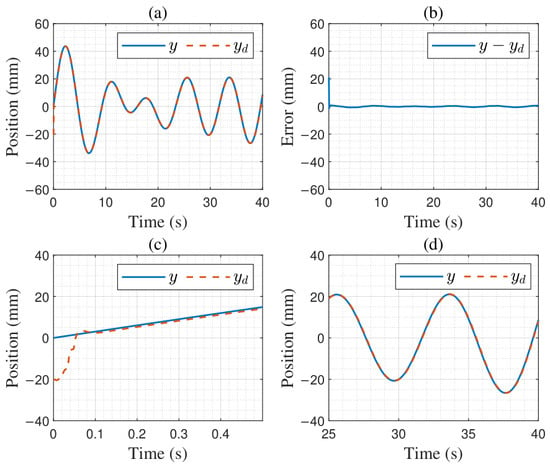
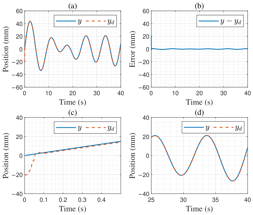
Figure 4 depicts the trajectory tracking output, error curve, transient response curve, and steady-state response curve of the system, where y represents the actual output trajectory and $y_d$ denotes the desired output trajectory. It is evident from the figures that the algorithm proposed in this chapter achieves excellent trajectory tracking performance with small errors and the tracking error is less than $0.75\mathrm{mm}$. This demonstrates that the proposed algorithm effectively compensates for the input time delay existing in the system, whereas the traditional algorithm lacks such compensation. The algorithm designed in this chapter can track the desired trajectory in about 0.09 s, and the system output trajectory basically coincides with the desired trajectory in the subsequent time. The traditional algorithm requires more time for tracking and has larger errors. In addition, a neural network is used to address model uncertainty and contribute to model feedforward compensation, leading the proposed method to achieve excellent tracking performance.

Figure 4. The EHSs tracking performance in simulation: (a) trajectory tracking; (b) tracking error; (c) transient state; (d) steady state.

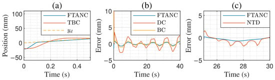
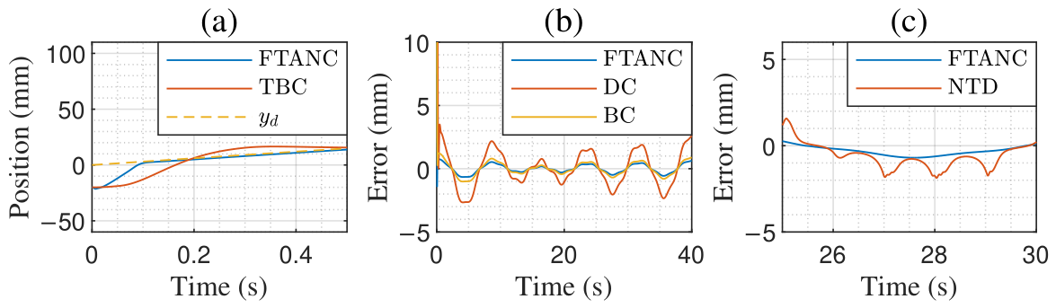
Figure 5 verifies the transient performance, robustness, and delay compensation effectiveness of the proposed FTANC scheme. As shown in Figure 5a, a faster convergence rate and higher tracking accuracy are achieved by FTANC compared with the traditional backstepping control (TBC). In Figure 5b, to verify the constraint capability for the first-order Padé approximation error, a 0.1 s delay expansion (DC) scenario and a pure backstepping control (BC) control group without neural network compensation are set; it can be clearly seen that significant error oscillation occurs in the DC and BC groups, based on which the maximum input delay that the proposed scheme can stably adapt to is determined to be 0.1 s. Meanwhile, the results confirm that the Padé approximation residual can be effectively constrained and compensated by the neural adaptation and finite-time robust mechanism of FTANC, the theoretical reliability of the extended fourth-order system is guaranteed, and strong robustness against delay variations and parameter uncertainties is exhibited. Combined with the adaptation range for small delays within 0.1 s, this algorithm can be applied to typical electro-hydraulic servo engineering scenarios such as hydraulic manipulators, load simulators, and rehabilitation exoskeletons. Figure 5c further confirms that the fluctuation of tracking error can be effectively suppressed by the Padé-based delay processing module, thus providing reliable support for high-precision trajectory tracking in the above scenarios.

Figure 5. The EHSs trajectory comparison of different control methods in simulation: (a) finite-time stability performance comparison; (b) minimal time-delay handling performance comparison; (c) RBFNNs performance comparison.

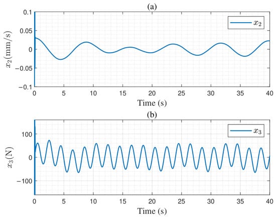
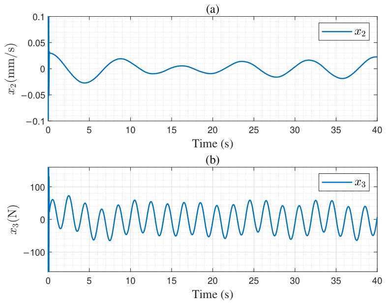
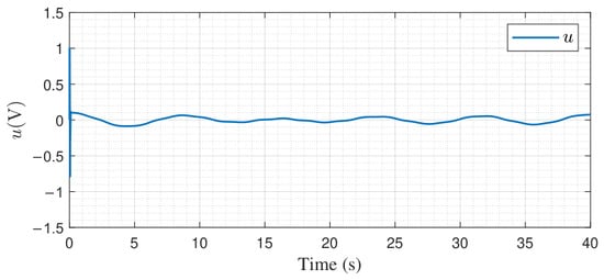
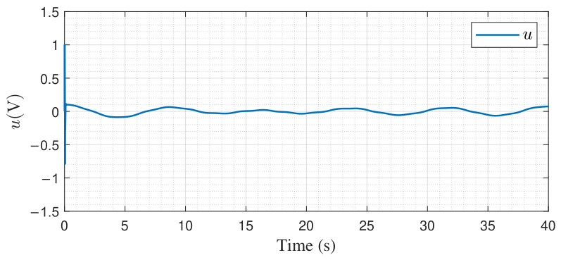
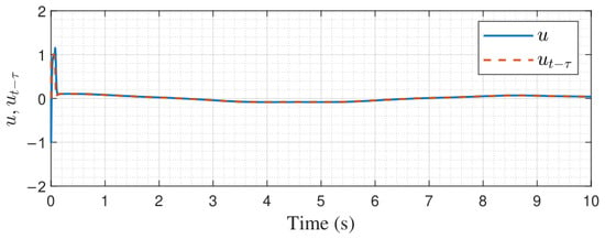
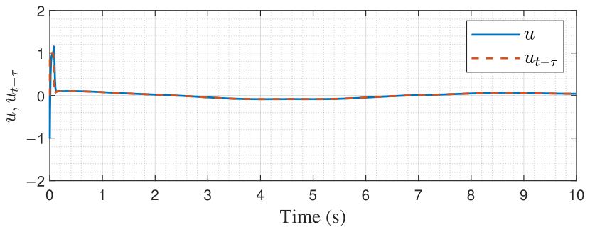
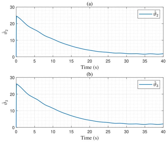
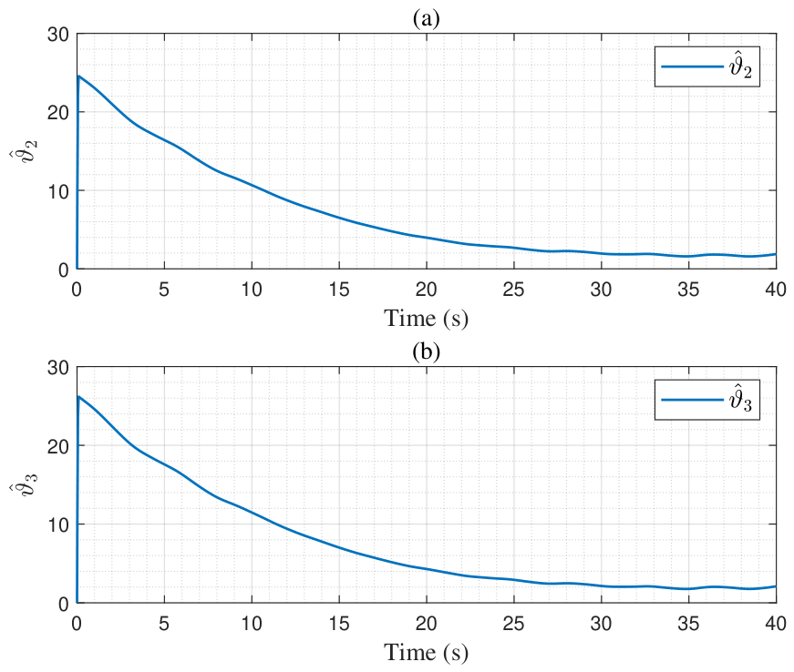
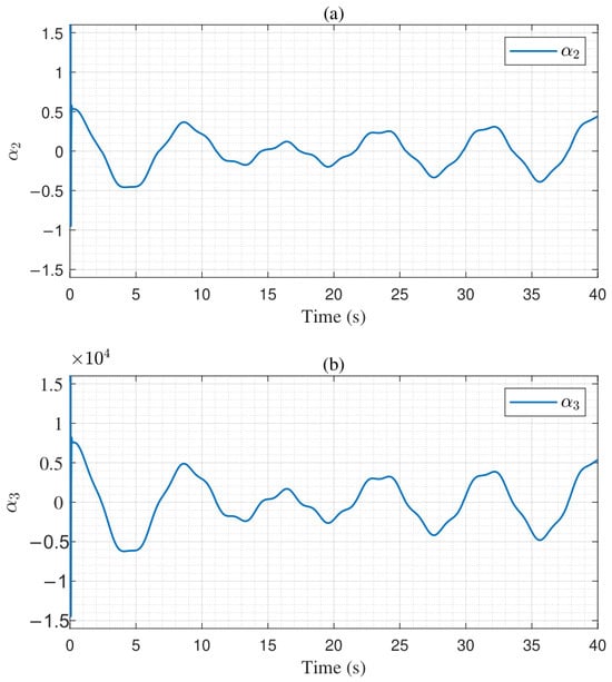
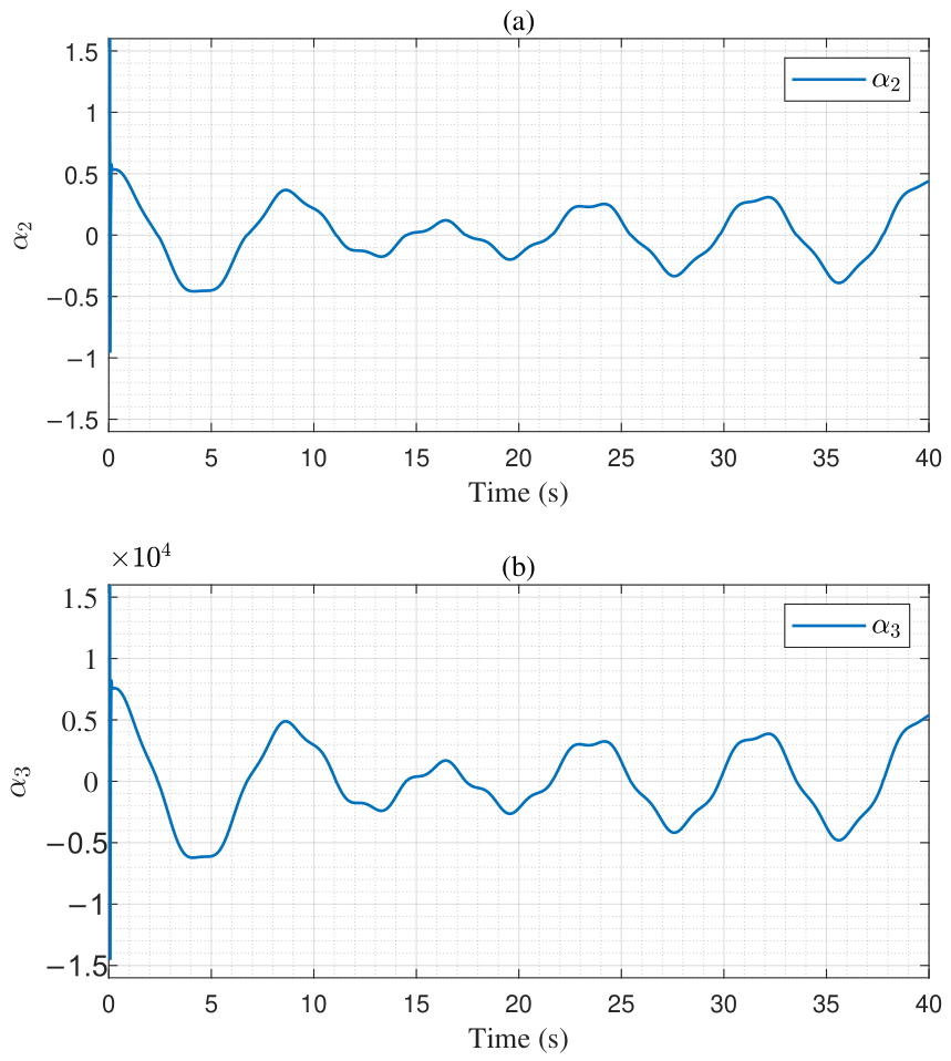
The system state responses $x_2$ and $x_3$ are presented in Figure 6, both exhibiting rapid convergence to bounded values. Due to the fast dynamic response of the F-EHSs, an initial overshoot is observed in $x_2$ and $x_3$, after which they quickly stabilize to a steady state. The associated control voltage, shown in Figure 7, remains a bounded signal throughout the response. Figure 8 shows the output value of the controller under the designed algorithm and the actual input value of the system, where u denotes the output value of the designed algorithm, and $u_{t-\tau }$ represents the actual input value to the electro-hydraulic servo valve after the system’s input time delay. In the simulation, this value is limited to $-2.4\mathrm{V}\le u,u_{t-\tau }\le 2.4\mathrm{V}$ to protect the system but the values do not reach the limit in the figure. The norm estimates of the RBFNNs weights for ${\widehat{\vartheta }}_2$ and ${\widehat{\vartheta }}_3$ are given in Figure 9, demonstrating rapid convergence to their respective steady states. Figure 10 shows the observation curves of the designed virtual control variables ${\alpha }_2$ and ${\alpha }_3$. It can be seen that the observation process converges rapidly to a steady state, indicating that the control algorithm has well stability and convergence.

Figure 6. The EHSs system states in simulation: (a) cylinder velocity; (b) load pressure response.

Figure 7. The control voltage of servo valve in simulation.

Figure 8. The contrast values of input control voltage in simulation.

Figure 9. The weight norm estimation of RBFNNs in simulation: (a) weight norm estimation for ${\mathrm{\Theta }}_2$; (b) weight norm estimation for ${\mathrm{\Theta }}_3$.

Figure 10. The virtual control variables in simulation: (a) ${\alpha }_2$ designed in the first backstepping recursive iteration; (b) ${\alpha }_3$ designed in the second backstepping recursive iteration.

5. Conclusions

In order to reduce the adverse effects of input delay and model uncertainty in EHSs, this study designs an adaptive controller capable of compensating for input time delay. First, addressing the input delay issue in EHSs, the Laplace transform combined with the Padé approximation method is employed to transform the delay term into an external parameter, effectively eliminating the impact of small delays. Subsequently, a neural network is employed to estimate matching and mismatching uncertainties, implementing feedforward compensation to ensure system convergence within finite time. Building upon this foundation, FTANC scheme is proposed by integrating traditional backstepping methods with finite-time stability theory. This approach guarantees rapid convergence of the system state to the zero neighborhood, even under non-zero initial conditions. Final simulation results validate the effectiveness of the FTANC approach, which significantly reduces the negative impact of small input delays while effectively enhancing tracking performance and system stability.

In future work, we will conduct research on EHSs with input dead-zone subject to input time delay. On the basis of the previous model, the input dead-zone characteristics will be added, followed by the observer design and controller design for this model. Meanwhile, distributed research on multiple electro-hydraulic servo systems will be carried out to further optimize the stability and tracking performance.

References

- Deng, W.; Zhou, H.; Zhou, J.; Yao, J. Neural network-based adaptive asymptotic prescribed performance tracking control of hydraulic manipulators. IEEE Trans. Syst. 2022, 53, 285–295. [Google Scholar] [CrossRef] [Scilit]
- Hall, A. The use of servo mechanisms in aircraft. J. Inst. Electr. Eng. Part I Gen. 1947, 94, 256–265. [Google Scholar] [CrossRef] [Scilit]
- Li, S.; Jiang, D.; Yan, Y.; Guo, Q. Synchronized control of multiple electrohydraulic systems with terminal sliding mode observer under parametric uncertainty and external load. ISA Trans. 2023, 133, 475–484. [Google Scholar] [CrossRef] [Scilit]
- Yang, Y.; Ma, L.; Huang, D. Development and repetitive learning control of lower limb exoskeleton driven by electrohydraulic actuators. IEEE Trans. Ind. Electron. 2017, 64, 4169–4178. [Google Scholar] [CrossRef] [Scilit]
- Li, J.; Kong, L.; Liang, H.; Li, W. Review of development and characteristics research on electro hydraulic servo system. Recent Patents Eng. 2024, 18, 140–154. [Google Scholar] [CrossRef] [Scilit]
- Biernacki, R.; Hwang, H.; Bhattacharyya, S. Robust stability with structured real parameter perturbations. IEEE Trans. Autom. Control 1987, 32, 495–506. [Google Scholar] [CrossRef]
- Chen, B.; Lee, T.; Feng, J. A nonlinear h control design in robotic systems under parameter perturbation and external disturbance. Int. J. Control 1994, 59, 439–461. [Google Scholar] [CrossRef] [Scilit]
- Meng, D.; Guo, T.; Xiang, R.; Wang, R.; Tan, J.; Wang, X.; Liang, B. An efficient solution method for workspace boundary of serpentine manipulators based on a unified kinematics model. IEEE Trans. Syst. Man Cybern. Syst. 2026, 56, 1790–1803. [Google Scholar] [CrossRef] [Scilit]
- Yu, D.; Ma, S.; Liu, Y.J.; Wang, Z.; Chen, C.P. Finite-time adaptive fuzzy backstepping control for quadrotor uav with stochastic disturbance. IEEE Trans. Autom. Sci. Eng. 2023, 21, 1335–1345. [Google Scholar] [CrossRef] [Scilit]
- Åström, K.J. Adaptive control. In Mathematical System Theory; Antoulas, A.C., Ed.; Springer: Berlin/Heidelberg, Germany, 1995; pp. 437–450. [Google Scholar] [CrossRef] [Scilit]
- Yang, Q.; Zhang, F.; Wang, C. Deterministic learning-based neural pid control for nonlinear robotic systems. IEEE/CAA J. Autom. Sin. 2024, 11, 1227–1238. [Google Scholar] [CrossRef] [Scilit]
- Hua, L.; Wang, W.; Shi, K.; Yang, J.; Zhong, Q.; Liang, H. Safety-critical fixed-time trajectory tracking of quadrotor uavs via event-triggered prescribed performance sliding mode control. IEEE Trans. Consum. Electron. 2026, 72, 1821–1830. [Google Scholar] [CrossRef] [Scilit]
- Wang, R.; Guo, T.; Li, Y.; Meng, D.; Liang, B. Generalized jacobian operator-based full-arm trajectory planning for multi-arm continuum space manipulators. Aerosp. Sci. Technol. 2025, 170, 111559. [Google Scholar] [CrossRef] [Scilit]
- Schwegel, M.; Glück, T.; Shaferman, V.; Zaccarian, L.; Kugi, A. Adaptive two-degrees-of-freedom current control for solenoids: Theoretical investigation and practical application. IEEE Trans. Control Syst. Technol. 2022, 31, 1078–1091. [Google Scholar] [CrossRef] [Scilit]
- Zhou, N.; Deng, Q.; Luo, W.; Huang, X.; Du, Y.; Chen, B.; Pedrycz, W. Correntropy meets cross-entropy: A robust loss against noisy labels. Eng. Appl. Artif. Intell. 2026, 167, 113830. [Google Scholar] [CrossRef] [Scilit]
- Zhou, N.; Luo, W.; Wu, Z.; Du, Y.; Shi, K.; Chen, B. Bipartite graph regularized robust low-rank matrix factorization for fast semi-supervised image clustering. Appl. Intell. 2026, 56, 22. [Google Scholar] [CrossRef] [Scilit]
- Luo, F.; Wang, S.; Lv, Y.; Mu, R.; Fo, J.; Zhang, T.; Xu, J.; Wang, C. Domain knowledge-enhanced graph reinforcement learning method for volt/var control in distribution networks. Appl. Energy 2025, 398, 126409. [Google Scholar] [CrossRef] [Scilit]
- Hou, Y.; Bai, B.; Zhao, S.; Wang, Y.; Wang, J.; Li, Z. Federated dynamic aggregation selection strategy-based multi-receptive field fusion classification framework for point cloud classification. Comput. Mater. Contin. 2026, 86, 1. [Google Scholar] [CrossRef] [Scilit]
- Hou, Y.; Zhao, S.; Xia, X.; Liwang, M.; Li, Z.; Xu, N.; Wu, D.; Tian, Y.; Quek, T.Q. Fedcdac: A federated clustering with dynamic aggregation and calibration method for sar image target recognition. IEEE J. Sel. Top. Appl. Earth Obs. Remote Sens. 2026, 19, 3726–3745. [Google Scholar] [CrossRef] [Scilit]
- Hou, Y.; Zhang, L.; Wang, J.; Li, H.; Duan, X.; Huang, K.; Tian, Y. Efficientsarnet: A light-weight, high performance and fast sar image target recognition network. IEEE Sens. J. 2026, 26, 11413–11431. [Google Scholar] [CrossRef] [Scilit]
- Hou, Y.; Yu, B.; Yang, Z.; Wang, J.; Xiang, W.; Wu, D.; Liwang, M.; Xia, X.; Li, Z.; Tian, Y.; et al. Privacy-preserving federated sar image target recognition with adaptive resource management in space-air-ground integrated networks. Pattern Recognit. 2026, 177, 113253. [Google Scholar] [CrossRef] [Scilit]
- Zhang, H.; Xu, J. Control for itô stochastic systems with input delay. IEEE Trans. Autom. Control 2016, 62, 350–365. [Google Scholar] [CrossRef] [Scilit]
- Fridman, E. A refined input delay approach to sampled-data control. Automatica 2010, 46, 421–427. [Google Scholar] [CrossRef] [Scilit]
- Liu, K.; Qiang, H.; Kang, S. Model predictive control of hydraulic drive unit considering input delay. Math. Methods Appl. Sci. 2021, 49, 1524–1542. [Google Scholar] [CrossRef] [Scilit]
- Yang, J.; Liang, H.; Shi, K.; Li, T. A class of matrix-valued function negative-determination method and its application to linear systems with time-varying delays. IEEE Trans. Syst. Man Cybern. 2026, 56, 988–998. [Google Scholar] [CrossRef] [Scilit]
- Yang, J.; Liang, H.; Wen, S.; Cheng, Y.; Huang, T. Aperiodic monotone-interval-partition approach for stability analysis of systems with time-varying delays. IEEE/CAA J. Autom. Sin. 2026; in press.
- Cao, Y.; Subhashri, A.R.; Chandrasekar, A.; Radhika, T.; Przybyszewski, K. Exponential state estimation for delayed competitive neural network via stochastic sampled-data control with markov jump parameters under actuator failure. J. Artif. Intell. Soft Comput. Res. 2024, 14, 373–385. [Google Scholar] [CrossRef] [Scilit]
- Bekiarisliberis, N.; Krstic, M. Compensation of state-dependent input delay for nonlinear systems. IEEE Trans. Autom. Control 2012, 58, 275–289. [Google Scholar] [CrossRef] [Scilit]
- Li, D.; Liu, Y.; Tong, S.; Chen, C.L.P.; Li, D. Neural networks-based adaptive control for nonlinear state constrained systems with input delay. IEEE Trans. Cybern. 2018, 49, 1249–1258. [Google Scholar] [CrossRef] [Scilit] [PubMed]
- Wang, S.; Luo, F.; Fo, J.; Lv, Y.; Wang, C. Two-stage spatiotemporal decoupling configuration of sop and multi-level electric-hydrogen hybrid energy storage based on feature extraction for distribution networks with ultra-high DG penetration. Appl. Energy 2025, 398, 126438. [Google Scholar] [CrossRef] [Scilit]
- Liu, Y.; Li, H.; Lu, R.; Zuo, Z.; Li, X. An overview of finite/fixed-time control and its application in engineering systems. IEEE/CAA J. Autom. Sin. 2022, 9, 2106–2120. [Google Scholar] [CrossRef] [Scilit]
- Hong, Y. Finite-time stabilization and stabilizability of a class of controllable systems. Syst. Control Lett. 2002, 46, 231–236. [Google Scholar] [CrossRef] [Scilit]
- Sui, S.; Chen, C.; Tong, S. Fuzzy adaptive finite-time control design for nontriangular stochastic nonlinear systems. IEEE Trans. Fuzzy Syst. 2018, 27, 172–184. [Google Scholar] [CrossRef] [Scilit]
- Yang, P.; Su, Y.; Zhang, L. Proximate fixed-time fault-tolerant tracking control for robot manipulators with prescribed performance. Automatica 2023, 157, 111262. [Google Scholar] [CrossRef] [Scilit]
- Yang, J.; Chen, G.; Wen, S.; Sheng, Y. Finite-time dissipative synchronization for state-dependent switching delayed neural networks via sampled-data control. Eng. Appl. Artif. Intell. 2025, 162, 112613. [Google Scholar] [CrossRef] [Scilit]
- Shi, T.; Hu, C.; Yu, J.; Wen, S. Fixed-time quantized synchronization of spatiotemporal networks with output-based quantization communication via boundary control. J. Frankl. Inst. 2025, 362, 107460. [Google Scholar] [CrossRef] [Scilit]
- Ma, L.; Hu, C.; Wen, S.; Yu, Z.; Jiang, H. Fixed-time distributed optimization via edge-based adaptive algorithms. IEEE Trans. Syst. Man Cybern. Syst. 2025, 55, 3436–3448. [Google Scholar] [CrossRef] [Scilit]
- Chen, Y.; Zhu, S.; Li, Y.; Liu, X.; Wen, S. Finite-time synchronization for delayed nns via generalized halanay inequalities. IEEE Trans. Syst. 2025, 55, 4742–4751. [Google Scholar] [CrossRef] [Scilit]
- Wang, C.; Wang, J.; Guo, Q.; Ren, X.; Cao, Y.; Jiang, D. Fixed-time adaptive neural control of electro-hydraulic system with model uncertainties: Theory and experiments. Control Eng. Pract. 2024, 147, 105931. [Google Scholar] [CrossRef] [Scilit]
- Guo, Q.; Zuo, Z.; Ding, Z. Parametric adaptive control of single-rod electrohydraulic system with block-strict-feedback model. Automatica 2020, 113, 108807. [Google Scholar] [CrossRef] [Scilit]
- Guo, Q. Optimal robust control of electro-hydraulic system based on hamilton–jacobi–bellman solution with backstepping iteration. IEEE Trans. Control Syst. Technol. 2022, 31, 459–466. [Google Scholar] [CrossRef] [Scilit]
- Yu, J.; Shi, P.; Zhao, L. Finite-time command filtered backstepping control for a class of nonlinear systems. Automatica 2018, 92, 173–180. [Google Scholar] [CrossRef] [Scilit]
- Sun, Y.; Wang, F.; Liu, Z.; Zhang, Y.; Chen, C.L.P. Fixed-time fuzzy control for a class of nonlinear systems. IEEE Trans. Cybern. 2020, 52, 3880–3887. [Google Scholar] [CrossRef] [Scilit] [PubMed]
- Deng, H.; Krstić, M. Stochastic nonlinear stabilizationłi: A backstepping design. Syst. Control Lett. 1997, 32, 143–150. [Google Scholar] [CrossRef] [Scilit]
- Wang, H.; Shen, L. Adaptive fuzzy fixed-time tracking control for nonlinear systems with time-varying full-state constraints and actuator hysteresis. IEEE Trans. Fuzzy Syst. 2022, 31, 1352–1361. [Google Scholar] [CrossRef] [Scilit]
- Song, X.; Wu, C.; Stojanovic, V.; Song, S. 1 bit encoding–decoding-based event-triggered fixedtime adaptive control for unmanned surface vehicle with guaranteed tracking performance. Control Eng. Pract. 2023, 135, 105513. [Google Scholar] [CrossRef] [Scilit]
Disclaimer/Publisher’s Note: The statements, opinions and data contained in all publications are solely those of the individual author(s) and contributor(s) and not of MDPI and/or the editor(s). MDPI and/or the editor(s) disclaim responsibility for any injury to people or property resulting from any ideas, methods, instructions or products referred to in the content. |
© 2026 by the authors. Licensee MDPI, Basel, Switzerland. This article is an open access article distributed under the terms and conditions of the Creative Commons Attribution (CC BY) license.