Exact and Heuristic Approaches for Weighted Throughput Maximization in Single-Machine Scheduling

Abstract

This study investigates a single-machine throughput maximization problem (TMP), in which each job is characterized by a processing time, ready date, due date, and weight, and must be completed within its time window to yield profit. The objective is to select and schedule a subset of jobs to maximize the total weight of completed jobs. While existing studies primarily focus on special cases or heuristic approaches, this paper develops a unified exact solution framework for the general TMP. The main contribution is a job-sorting-based approach in which dominance rules are derived from structural properties induced by a partial ordering, while a complete ordering based on time-window midpoints is used to guide job sequencing. Based on this framework, several solution approaches are developed, including implicit enumeration (IE) methods, branch-and-bound (B&B) methods enhanced with linear programming (LP) relaxation, and a mixed-integer programming (MIP) model. A heuristic method is also proposed to generate high-quality initial solutions that accelerate exact methods. Computational experiments are conducted on a comprehensive set of instances. The results demonstrate that the proposed job sorting and dominance rules significantly improve computational efficiency, leading to substantial reductions in solution time compared with baseline methods.

1. Introduction

Scheduling plays a critical role in production and operations management, where limited resources must be allocated efficiently to competing tasks. In many real-world environments, decision makers must determine not only how to schedule jobs, but also which jobs to select for processing in order to maximize overall profit or system performance. This leads to the throughput maximization problem (TMP), also known as the order selection problem, in which a subset of jobs is chosen and scheduled within given time constraints.

This study considers the single-machine TMP in which each job is characterized by a ready date, due date, processing time, and weight. A job must be fully processed within its time window to earn its associated payoff; otherwise, it is rejected. The objective is to maximize the total weight of completed jobs. Such problems arise in various production settings, particularly in make-to-order environments where capacity is limited and jobs differ in profitability and timing requirements.

Although real-world production systems often involve multiple machines, single-machine models remain valuable for tactical capacity planning and bottleneck scheduling. In long-term planning, machines with similar functionalities are frequently aggregated into a single capacity resource to evaluate feasibility [1]. Furthermore, many small and medium-sized companies are centered around a dominant bottleneck machine whose capacity largely determines overall system performance. In such cases, single-machine scheduling models provide a robust framework for analyzing capacity feasibility and developing efficient scheduling algorithms. Recent survey studies, such as Martinelli et al. [2] and Ying et al. [3], further highlight the continued relevance and ongoing development of single-machine production scheduling in theoretical research and real-world applications.

In real-world settings, manufacturers often face the critical task of maximizing profit by selecting a subset of orders from a candidate pool such that the chosen orders can be feasibly scheduled. In this study, the terms “order” and “job” are used interchangeably. A solution to this problem must specify both the subset of jobs to be processed and their corresponding production schedule. Such scenarios commonly arise in production environments such as apparel manufacturing, where orders have distinct selling seasons and material lead times. Additionally, due to high setup costs and time constraints, splitting an order across multiple production periods is impractical; therefore, preemption is prohibited. Moreover, partial fulfillment is not permitted, as an order must be either fully completed or entirely rejected. Since some garments feature high-fashion designs while others target price-sensitive markets, the potential profit varies substantially across different orders.

Despite extensive research on TMP and related scheduling problems, most existing studies focus on special cases, extended models with additional constraints, or heuristic approaches for large-scale instances. Comparatively fewer studies address the general TMP with time windows and job selection decisions using efficient exact methods.

To address this gap, this paper develops several solution approaches, including an MIP model, a partial-ordering-based (⇒) heuristic sorting method, an IE approach with dominance rules, and a B&B method enhanced by LP-relaxation. Computational experiments are conducted to evaluate the effectiveness and efficiency of the proposed methods. The following example illustrates the constraints and objectives of the TMP.

• Illustration Example

There are six jobs in this example. The ready date and the due date (time window) of these jobs are shown in Figure 1. The optimal set of selected jobs is {1, 2, 4, 5, 6} and an optimal schedule is shown as a Gantt Chart on the time axis at the bottom of the figure. There are only three cases of time window overlap; they are between Jobs 1 and 2, between Jobs 3 and 4, and between Jobs 5 and 6; hence, this problem can be treated as three independent problems. Observing the figure, moving the processing of Job 1 later will make the time insufficient for processing Job 2. Hence, Job 1 should start at $r_1$ and Job 2 is processed right after Job 1 is completed. That $w_3<w_4$ is assumed in this example. The ready date of Job 3 is earlier than that of Job 4. However, scheduling Job 3 will make the more profitable Job 4 impossible to be produced. Consequently, one should make the machine idle between interval $\left[r_3, r_4\right]$ and schedule Job 4 starting at $r_4$. Assume $w_5<w_6$. Jobs 5 and 6 have an identical ready date, selecting the more profitable Job 6 to start at its ready time makes Job 5 impossible to be scheduled. However, processing Job 5 before Job 6 will make the production of both jobs feasible. The above solutions to the three subproblems are not only feasible but also optimal.

The remainder of this paper is organized as follows. Section 2 reviews the relevant literature. Section 3 presents the problem formulation. Section 4 describes the proposed solution approaches. Section 5 and Section 6 report computational experiments and results, respectively. Section 7 concludes the paper.

2. Literature Review

2.1. Classical Throughput Maximization Problem

The TMP is a scheduling problem that aims to maximize the total weight of selected jobs. Several studies have investigated this problem under various assumptions regarding job attributes. Karp [4] proved that a special case, in which all jobs have identical ready dates ($r_j=r$), is NP-hard. Subsequently, Sahni [5] proposed a dynamic programming (DP) approach to solve this special case. In recent years, research on scheduling has also explored emerging methodologies, including artificial intelligence–based approaches. For example, Bouška et al. [6] and Liu et al. [7] investigated the application of learning-based techniques to scheduling problems.

2.2. Variants Based on Job Attributes

Various extensions of TMP have been studied by modifying job-related attributes, such as processing times, penalties, and resource requirements. Considering a variation where job weights are reduced by lateness penalties, Slotnick and Morton [8] developed a B&B method to identify optimal solutions, along with two heuristic methods for generating approximate solutions. Ghosh [9] subsequently proved that the problem studied by Slotnick and Morton is NP-hard. Building on these results, Slotnick and Morton [10] and Juraszek [11] extended the model by replacing the lateness penalty with a tardiness penalty. Slotnick and Morton [10] formulated the problem as an integer program and proposed a B&B method that incorporates LP-relaxation for bounding, in addition to heuristic approaches. Juraszek and Malgorzata [11] addressed the same problem in a multi-machine environment using an MIP model. They proposed a B&B algorithm, a simulated annealing (SA) heuristic, and a list scheduling algorithm to generate initial solutions for both the B&B and SA methods.

In the TMP, a job is considered eligible only if its processing time $p_j$ is no longer than its time window $R_j$. The portion of a time window not occupied by processing is defined as slack time. Arkin and Silverberg [12] examined a special case in which no slack time exists for any job under a multi-machine setting and proposed a DP model for the problem. Later, Calinescu et al. [13] studied the same problem in a single-machine environment, introducing a DP algorithm suitable for large-scale problems, along with a randomized rounding algorithm and a list-based algorithm for small-scale instances.

If all jobs must be selected and processed, the TMP becomes equivalent to the problem of minimizing the weighted number of tardy jobs [14]. Several researchers have investigated this related problem in previous studies. Lawler and Moore [15] first examined a special case in which all jobs have identical ready dates. Subsequently, Lawler [16] considered a case where job processing times and weights are ordered in opposite directions. Kise et al. [17] analyzed a special case under specific assumptions on ready and due dates, where the order of ready dates matches the order of due dates for all jobs. They also proposed a DP algorithm to solve this case. In another special case, Lawler [18] developed a DP algorithm for problems in which all job weights are identical and preemption is permitted.

Several studies have focused on special cases regarding job processing times. Baptiste [19] considered a scenario in which all jobs have identical processing times and proposed a DP algorithm with a time complexity of $O\left(n^7\right)$, where $n$ is the number of jobs, under the assumption that preemption is not permitted. For the preemptive case, the problem was shown to be solvable in $O\left(n^{10}\right)$ time. Subsequently, Baptiste et al. [20] improved these results by presenting an algorithm with a reduced time complexity of $O\left(n^4\right)$ for the preemptive case originally studied by Baptiste [19].

A special case in which a job can be completed in a shorter duration by increasing resource usage at a higher cost is defined as the controllable processing time problem [21]. Yang and Geunes [14] investigated the single-machine TMP under the assumption of controllable processing times, where a tardiness cost is incurred if a job is completed after its due date. The TMP that incorporates both controllable processing times and tardiness penalties is known as the job selection with controllable processing times and tardiness scheduling problem. Yang and Geunes also proposed heuristic approaches to solve this problem.

In modern high-tech manufacturing environments, the profit obtained from completing a job may vary over time. Many products, such as memory chips and computers, have short life cycles and rapidly declining selling prices. To account for decreasing profits, Yang [22] assumed that the profit generated by a job decreases exponentially with its completion time and developed both a B&B algorithm and a heuristic method to address this problem. Furthermore, addressing scenarios with time-sensitive revenue and operational complexities, Chaurasia and Singh [23] investigated the single-machine problem with release dates and sequence-dependent setup times. Such setup times commonly occur when different jobs require distinct setup procedures. To solve their model, they proposed a hybrid steady-state genetic algorithm and an evolutionary algorithm with guided mutation.

Silva et al. [24] studied scheduling problems involving processing times, release dates, due dates, deadlines, revenues, and penalties. They proposed two exact algorithms: one based on Lagrangian relaxation and the other based on column generation. Both methods effectively handle sequence-dependent setup times and complex job constraints. Li and Ventura [25] also focused on single-machine order acceptance and scheduling (OAS) problems with revenues, due dates, and tardiness costs. They developed three exact algorithms: the first based on DP, the second employing a staged DP with gradual constraint recovery, and the third incorporating Lagrangian relaxation to enhance performance. Further exploring the single-machine OAS problem, de Weerdt et al. [26] addressed scheduling with release times, deadlines, setup times, and job rejection. They proposed an exact algorithm that is fixed-parameter tractable based on slack and width, where width refers to the number of overlapping time windows. Tarhan and Oğuz [27] introduced a metaheuristic approach for the OAS problem in a single-machine, make-to-order setting with release times and sequence-dependent setup times. Their method integrates a time-bucket-based MIP model with variable neighborhood search and tabu search.

Under the Just-in-Time (JIT) philosophy, jobs are often required to be completed exactly on their due dates to avoid both earliness and tardiness penalties. Gerstl and Mosheiov [28] addressed scheduling problems in such environments by proposing a DP algorithm to maximize the weighted number of JIT-compliant jobs for a given job sequence. These problems were shown to be solvable in polynomial time for both identical and unrelated machine settings.

More recently, Kaul et al. [29] studied a single-machine scheduling problem of time-window jobs with the objective of minimizing the number of tardy jobs.

2.3. Machine Environments of TMP

In addition to job-related variations, TMP has also been extended to different machine environments. By distinguishing between machine types (identical vs. unrelated) and job weight types (identical vs. arbitrary), Bar-Noy et al. [30] considered four variants of the TMP and proposed constant-factor approximation algorithms based on LP to solve each variant. They also presented a combinatorial algorithm to solve the TMP under the setting of arbitrary job weights and unrelated machines. Building on this work, Berman and Dasgupta [31] developed combinatorial algorithms that do not rely on LP and are significantly faster than the method proposed by Bar-Noy et al. [30]. Motivated by the work of Baptiste [19], Chuzhoy et al. [32] studied the TMP in both single-machine and multi-machine environments and proposed a DP algorithm. Zhang and Lu [33] addressed a parallel-machine scheduling problem that incorporates release dates and allows job rejection. They proposed a DP algorithm and a fully polynomial-time approximation scheme (FPTAS) to minimize the sum of the makespan and the total penalty incurred from rejected jobs.

Focusing on an unrelated parallel machine environment where all jobs are assumed to have a ready time of zero ($r_j$ = 0), Wang and Ye [34] developed two MIP models and a formulation-based B&B algorithm for the OAS problem. Wang et al. [35] extended this work by considering additional complexities, such as machine-dependent setup times and maximum machine availability, to maximize total revenue while accounting for costs associated with the makespan. They proposed a two-layer logic-based Benders decomposition method, which decomposes the problem into an acceptance master problem and assignment-sequencing subproblems.

For the problem of minimizing makespan on unrelated parallel machines with sequence-dependent setup times, Fanjul-Peyró et al. [36] introduced a mathematical programming-based algorithm that employs two different MIP models (one for machine selection and the other for sequencing) while iteratively incorporating results as lower bounds. Addressing the OAS problem with time windows and sequence-dependent setup times on unrelated parallel machines, Mahmoudinazlou et al. [37] proposed a hybrid population-based heuristic that combines an Imperialist Competitive Algorithm with simulated annealing. Considering sequence-dependent setup times in an unrelated parallel-machine environment, Jos et al. [38] proposed three MIP models: one precedence-based, one position-based, and one time-indexed.

2.4. Online Throughput Maximization

Another important research direction considers online versions of the TMP, where job information is not known in advance. In real-world environments where jobs arrive sequentially and their attributes are unknown in advance, the scheduling problem becomes an online problem. This setting requires dynamically generating a sequence of decisions to assign resources to tasks in real time. Consequently, schedulers must often make decisions based solely on information available from jobs that have already arrived. Baruah et al. [39] and Koren and Shasha [40] studied online scheduling problems with preemption, while Lipton and Tomkins [41] examined the non-preemptive version. Chin et al. [42] investigated an online scheduling problem arising from network buffer management. They assumed that all jobs have identical processing times, that ready dates and due dates are integers, and that weights are real numbers. A randomized algorithm was proposed to solve the problem under these assumptions. Liu et al. [43] deal with online and offline versions of the job selection or rejection problem.

2.5. Applications of TMP

Beyond theoretical developments, TMP has also been applied to various practical domains. Bar-Noy et al. [44] presented a general framework for solving the TMP and applied it to various domains, such as bandwidth allocation for sessions in communication networks and dynamic storage allocation. Subsequently, Bar-Noy et al. [45] considered the TMP with batching in a multi-machine environment, where jobs are grouped into several families. Each family is associated with a specific processing time, and jobs belonging to the same family can be batched and processed together on a single machine. The processing time of each batch is equal to the processing time assigned to its job family. The batch scheduling methods proposed by Bar-Noy et al. [45] have been applied to practical problems, including client scheduling in multimedia-on-demand systems and thermal treatment scheduling for multi-layer ceramic packaging.

Despite the extensive literature on TMP, most existing studies focus on special cases, extended models with additional constraints (e.g., sequence-dependent setup times, controllable processing times), or heuristic approaches for large-scale instances. Comparatively fewer studies address the general single-machine TMP with ready dates, due dates, and job selection decisions using efficient exact methods.

To the best of our knowledge, no existing study investigates the TMP under the exact set of assumptions considered in this paper. The works of Og et al. [46] and Mahmoudinazlou et al. [37] are the most closely related; however, their models incorporate sequence-dependent setup times, which are not considered in this study. Furthermore, while these studies primarily emphasize heuristic or metaheuristic approaches, the present study focuses on the development of exact optimization methods.

Specifically, this paper investigates several solution approaches, including a partial-ordering-based heuristic sorting method, an IE approach with dominance rules, and a B&B method enhanced by LP-relaxation and an MIP model. The proposed approaches provide both theoretical insights and practical solution techniques for solving the TMP efficiently under realistic time-window constraints.

3. Problem Description

We now formally define the problem. Let $n$ be the total number of jobs, where each job $j$ is characterized by four attributes: its ready date $r_j$, due date $d_j$, processing time $p_j$, and weight $w_j$. The time interval $[r_j,d_j]$, denoted as $R_j$, is defined as the time window of job $j$; the length of $d_j-r_j$ is denoted by $\left|R_j\right|$. A job must be processed within its time window $[r_j,d_j]$ without preemption, and no payoff is granted for tardy or partially completed jobs. Following the three-field notation of Graham et al. [47], the TMP considered in this study can be represented as $1/{ r}_j, d_j /{\sum }_{j\in J}{w}_j{I}_j$. Here, $j\in J$ represents the set of all jobs, and $I_j$ is a binary decision variable that equals 1 if job $j$ is selected and completed within its time window, and 0 otherwise.

This study distinguishes between the terms solution and schedule. A solution specifies a subset of selected jobs and their processing sequence but does not define exact start times. In contrast, a schedule explicitly defines the start and end times for each selected job. A job is feasibly scheduled if its start time is no earlier than its ready date ($r_j$) and its completion time is no later than its due date ($d_j$). Accordingly, a solution is deemed feasible if all selected jobs can be scheduled within their respective time windows in the specified sequence. Since the objective value, the total weight of selected jobs, is independent of specific start and end times, multiple feasible schedules may correspond to the same feasible solution. This occurs because job start and end times can often be shifted within their allowable windows without violating feasibility. An optimal solution is defined as a feasible solution whose total weight is at least as large as that of any other feasible solution. The focus of this study is to identify a single optimal solution rather than enumerating all alternative optima.

The degree of overlap among job time windows reflects the difficulty level of the scheduling problem. A TMP instance with no overlap between any pair of job time windows is the most trivial case. In such scenarios, selecting all jobs and scheduling each within its respective time window yields an optimal solution. In contrast, the most difficult case arises when all jobs share identical time windows, such that $r_j=r$ and $d_j=d, \forall j\in J$. This version of TMP is equivalent to the classical knapsack problem. By treating each job as an item, the common time window length as the knapsack capacity, the job processing time as the item weight, and the job weight as the item value, TMP can be transformed into a knapsack problem. The knapsack problem was proven to be NP-hard by Mathews [48]. Furthermore, Karp [4] demonstrated that TMP is NP-hard even when all jobs share the same ready date. Since both of these problems can be reduced to the TMP investigated in this study, the complexity of TMP ranges from a trivial case to a difficult NP-hard problem, depending on the degree of time window overlap.

The TMP can be formulated as the following optimization problem:

$$\mathrm{Maximize} {\sum }_{j\in J}{w}_j{I}_j$$

(1)

subject to scheduling feasibility constraints that ensure:

• Each selected job is processed within its time window $[r_j,d_j]$;
• No two jobs overlap in processing on the single machine,
• Processing is non-preemptive.

Here, $I_j\in \{0, 1\}$ indicates whether job $j$ is selected and completed.

The following assumptions are adopted in this study:

• Jobs are processed on a single machine;
• Preemption is not allowed;
• Each job must be completed within its time window to earn its weight;
• The machine can process at most one job at a time;
• All job parameters are known in advance.

4. Solution Approaches

Two major classes of approaches are commonly used to solve NP-hard scheduling problems. The first category consists of exact methods, which systematically explore the solution space to identify an optimal solution, typically through enumeration or mathematical optimization techniques. The second category includes heuristic methods, which aim to generate high-quality solutions within limited computation time.

This study focuses on the development of exact methods based on an enumeration framework. In particular, several solution approaches are proposed and compared, including an MIP model solved by Gurobi version 7.5, an IE method, and a B&B method enhanced with midpoint-based ordering, dominance rules, and LP-relaxation. A heuristic method is also developed to generate initial feasible solutions and support the exact approaches.

Almost all exact combinatorial optimization methods, including commercial integer programming solvers, rely on enumeration combined with techniques that reduce the size of the search tree and, consequently, the computational burden. The main contribution of this paper is the development of a job-sorting-based framework in which dominance rules are derived from structural properties induced by a partial ordering (⇒), while a complete ordering based on time-window midpoints is used to guide job sequencing. To evaluate this contribution, an enumerative method incorporating midpoint-based ordering and dominance rules is compared with a pure enumerative method. When these two enumerative approaches are further enhanced with LP relaxation at each explored node, they become B&B methods. In addition, a heuristic method that rapidly generates feasible solutions is used to provide improved lower bounds, thereby accelerating the B&B process. The heuristic solutions can also be supplied to the MIP solver as initial solutions to enhance its performance. Figure 2 illustrates the five solution approaches compared in this study, as well as the relationships among them and the development flow of the proposed techniques.

Section 4.1 introduces the heuristic method. Section 4.2 presents the MIP model. Section 4.3 details the IE method, which incorporates four dominance rules to prune the search tree and reduce computation time. Section 4.4 presents an LP relaxation formulation used to solve subproblems at nodes in the B&B enumeration tree.

4.1. Heuristic Method

The focus of this heuristic method is to prioritize jobs based on their payoff per unit of processing time. The weight rate of job j, denoted by ${\rho }_j^W$, is defined as

$${\rho }_j^W={\displaystyle \raisebox{1ex}{$w_j$}\!\left/ \!\raisebox{-1ex}{$p_j$}\right.}$$

(2)

where $w_j$ is the weight and $p_j$ is the processing time of job $j$. Hence, ${\rho }_j^W$ represents the weight per unit of processing time.

The capacity demand rate of job $j$, denoted by ${\rho }_j^{CD}\left(t\right)$, is defined as a time-dependent function:

$${\rho }_j^{CD}\left(t\right)=\left\{\begin{array}{c}{\displaystyle \raisebox{1ex}{$p_j$}\!\left/ \!\raisebox{-1ex}{$(d_j-r_j)$}\right.}, \mathrm{if} r_j\le t\le d_j\\ 0, \mathrm{otherwise}\end{array}\right.,$$

(3)

where ${\displaystyle \raisebox{1ex}{$p_j$}\!\left/ \!\raisebox{-1ex}{$(d_j-r_j)$}\right.}$ represents the average processing requirement per unit of time over the time window $\left[r_j,d_j\right]$ of job $j$.

The overall capacity demand rate at time $t$, aggregated across all jobs, is defined as:

$${\overline{\rho }}^{CD}\left(t\right)={\sum }_{j=1}^n{\rho }_j^{CD}\left(t\right),$$

(4)

which represents the total processing load at time $t$.

The heuristic prioritizes jobs based on their weight rates ${\rho }_j^W$. Specifically, all jobs are initially sorted in descending order of ${\rho }_j^W$, so that jobs with higher payoff per unit processing time are considered earlier for inclusion in the schedule.

Given a partially constructed solution, a candidate job can be inserted into several possible slots: before the first job, between any two consecutive jobs, or after the last job in the current sequence. To maximize the available space within a specific slot for potential insertion, jobs scheduled before the slot are shifted as early as possible, while those scheduled after the slot are shifted as late as possible. This is achieved by calculating the earliest completion times for the jobs preceding the slot and the latest start times for the jobs following the slot.

Let $\left[j\right]$ be the job at position $j$ in the current sequence $H$, and let $r_{\left[j\right]}$, $p_{\left[j\right]}$, and $d_{\left[j\right]}$ be its ready date, processing time, and due date, respectively. Let $C_{\left[j\right]}^E$ and $S_{\left[j\right]}^L$ denote the earliest completion time and the latest start time of job $\left[j\right]$, respectively. Furthermore, let $n\left(H\right)$ be the number of jobs currently scheduled in $H$.

Let $s$ denote the index of a slot. Slot $s$ refers to the position before the $s$-th job in the current schedule. Specifically, slot 1 is located before the first job, while slot $n\left(H\right)+1$ corresponds to the position after the last scheduled job, where $n\left(H\right)$ represents the number of jobs currently in the sequence $H$. Consider job $j$ for insertion into slot $s$.

For a candidate job $j$ to be inserted into slot $s$, a feasible time window $R_{j,s}^{\prime }$ is defined. This window represents the allowable interval in which job $j$ can be scheduled, constrained by its ready date $r_j$, due date $d_j$, and the time availability between adjacent jobs in the current schedule. The interval $R_{j,s}^{\prime }$ is computed as follows:

• If $s=1$ (before the first job): $R_{j,s}^{\prime }$ = $[r_j,\mathrm{m}\mathrm{i}\mathrm{n}(S_{\left[s\right]}^L,d_j\left)\right]$
• If $1<s<n\left(H\right)+1$ (between two jobs): $R_{j,s}^{\prime }$ = $[\max \left(C_{\left[s-1\right]}^E,r_j\right),\mathrm{m}\mathrm{i}\mathrm{n}(S_{\left[s\right]}^L,d_j\left)\right]$
• If $s=n\left(H\right)+1$ (after the last job): $R_{j,s}^{\prime }$ = $[\max \left(C_{\left[n\left(H\right)\right]}^E,r_j\right),d_j]$

The length of this time window is denoted as $\left|R_{j,s}^{\prime }\right|$. If $\left|R_{j,s}^{\prime }\right|$ < $p_j$, where $p_j$ is the processing time of job $j$, then job $j$ cannot be inserted into slot $s$. If no slot has sufficient space, then job $j$ is excluded from the current schedule, and the next job in the sorted list (based on weight rate) is evaluated.

To determine the best slot for a candidate job, the heuristic evaluates each feasible slot based on the average capacity requirement within its allowable window $R_{j,s}^{\prime }$. The average capacity demand ${\chi }_{j,s}$ is calculated by integrating the total demand curve ${\int }_{R_{j,s}^{\prime }}{\overline{\rho }}^{CD}\left(t\right)dt$ over the interval $R_{j,s}^{\prime }$ and dividing the result by the window length $\left|R_{j,s}^{\prime }\right|$:

$${\chi }_{j,s}={\displaystyle \raisebox{1ex}{${\int }_{R_{j,s}^{\prime }}{\overline{\rho }}^{CD}\left(t\right)dt$}\!\left/ \!\raisebox{-1ex}{$\left|R_{j,s}^{\prime }\right|$}\right.}$$

(5)

This metric reflects the average processing load within the potential insertion interval. The slot with the minimum average capacity demand ${\chi }_{j,s}$ is selected for inserting the job. This criterion identifies the slot that is the least congested in terms of competing job demands within its feasible time window.

4.2. MIP Model

To provide a benchmark and enable comparison with general-purpose optimization approaches, the TMP is formulated as an MIP model. The formulation captures both job selection and sequencing decisions within a unified framework. Unlike the proposed enumeration-based methods, which exploit problem-specific structural properties, the MIP model is solved using a commercial solver and serves as a baseline for evaluating solution quality and computational performance.

The MIP model is presented here in Formulation 1.

Formulation 1.
Sets and Indices
$J$: set of all jobs.
$i,j$$: \mathrm{index} \mathrm{of} \mathrm{jobs}, i,j\in J.$
Decision variables
$I_j$$: \mathrm{Binary} \mathrm{variable}, \mathrm{where} I_j=1$$\mathrm{if} \mathrm{job} j$$\mathrm{is} \mathrm{selected} \mathrm{and} 0 \mathrm{otherwise}, \forall j\in J.$
$Y_{ij}$$: \mathrm{Binary} \mathrm{variable} \mathrm{for} \forall i,j\in J$$\mathrm{and} i<j.$$\mathrm{When} \mathrm{both} \mathrm{jobs} i$$\mathrm{and} j$$\mathrm{are} \mathrm{selected}, Y_{ij}=1$$\mathrm{indicates} \mathrm{that} \mathrm{job} i$$\mathrm{is} \mathrm{scheduled} \mathrm{before} \mathrm{job} j,$$\mathrm{while} Y_{ij}=0$$\mathrm{indicates} \mathrm{that} \mathrm{job} j$$\mathrm{is} \mathrm{scheduled} \mathrm{before} \mathrm{job} i.$
$S_j$$: \mathrm{Continuous} \mathrm{variable} \mathrm{denoting} \mathrm{the} \mathrm{start} \mathrm{time} \mathrm{of} \mathrm{job} j,$$\forall j\in J.$$\mathrm{The} \mathrm{completion} \mathrm{time} \mathrm{of} \mathrm{job} j$$\mathrm{is} \mathrm{thus} \mathrm{defined} \mathrm{as} S_j+p_j.$
$M$: A sufficiently large positive constant.
Objective Function
$\mathrm{Maximize} {\sum }_{j\in J}{w}_j{I}_j$	(6)
Subject to
$r_j\le S_j, \forall j\in J$	(7)
$S_j+p_j\le d_j, \forall j\in J$	(8)
$S_j\ge \left(S_i+p_i\right)-M\left(1-Y_{ij}\right)-M\left(1-I_i\right)-M\left(1-I_j\right), \forall i,j\in J, i<j$	(9)
$S_i\ge \left(S_j+p_j\right)-M{Y}_{ij}-M\left(1-I_i\right)-M\left(1-I_j\right), \forall i,j\in J, i<j$	(10)
$Y_{ij}\in \{0, 1\}, \forall i,j\in J, i<j$	(11)
$I_j\in \{0, 1\}, \forall j\in J$	(12)

Formulation 1 presents a MIP model for the considered scheduling problem. The objective function (6) aims to maximize the total weight of the selected jobs. Constraint (7) ensures that the start time of each job is no earlier than its ready date. Constraint (8) enforces that the completion time of each job does not exceed its due date. Constraints (9) and (10) manage the precedence relationships between any two selected jobs; specifically, if two jobs are selected, one must precede the other. Constraints (11) and (12) specify that $Y_{ij}$ and $I_j$ are binary variables, respectively. In Formulation 1, the number of continuous variables $S_j$ and binary variables $I_j$ is $n$ each, while the number of binary variables $Y_{ij}$ is ${\displaystyle \frac{n(n-1)}{2}}$. Solving this MIP yields an optimal solution to the TMP. The heuristic method introduced in Section 4.1 can be used to generate an initial feasible solution to facilitate the MIP solving process. This MIP model is solved by Gurobi [49] in the experiment results presented in Section 6.

4.3. IE Approach

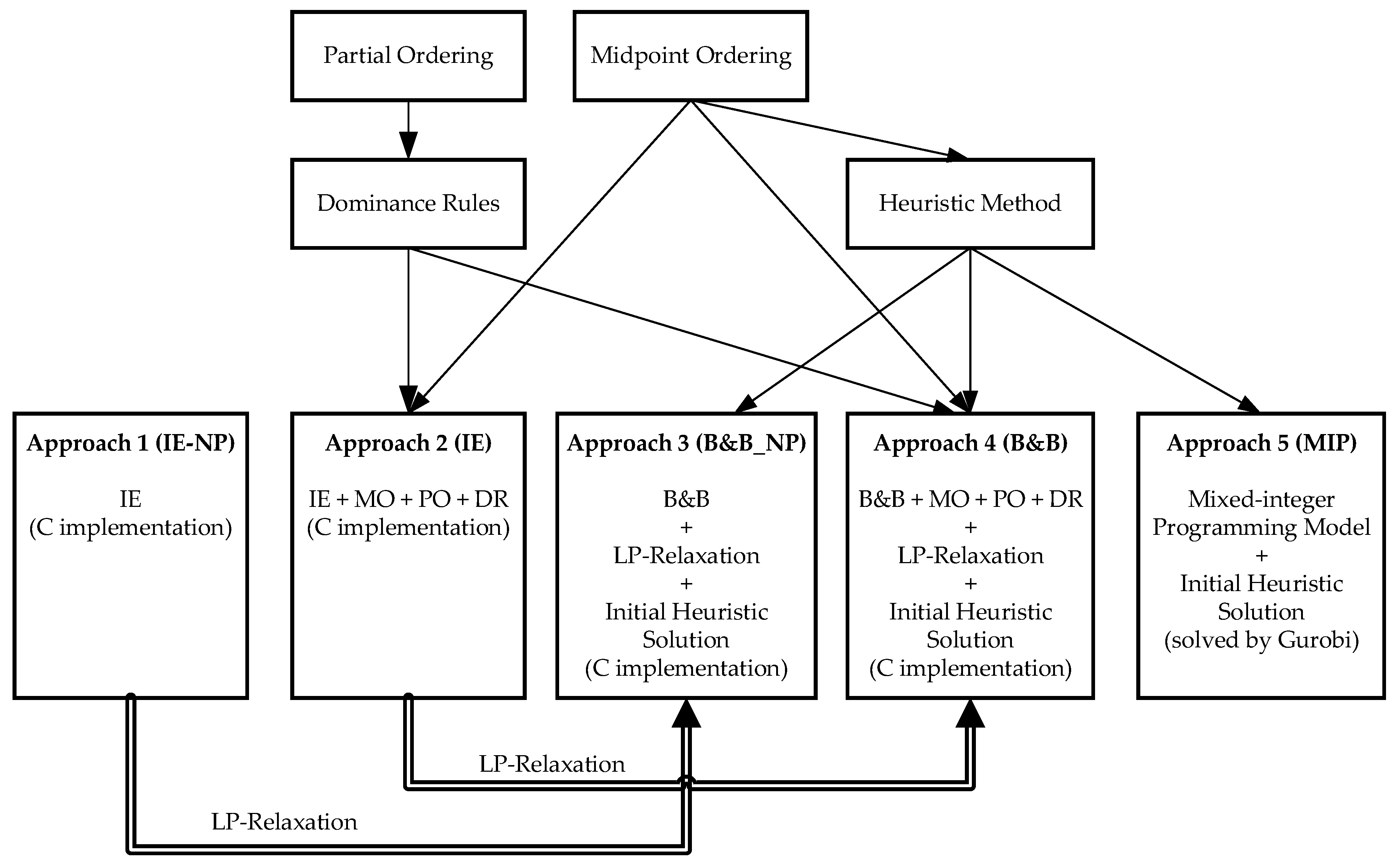
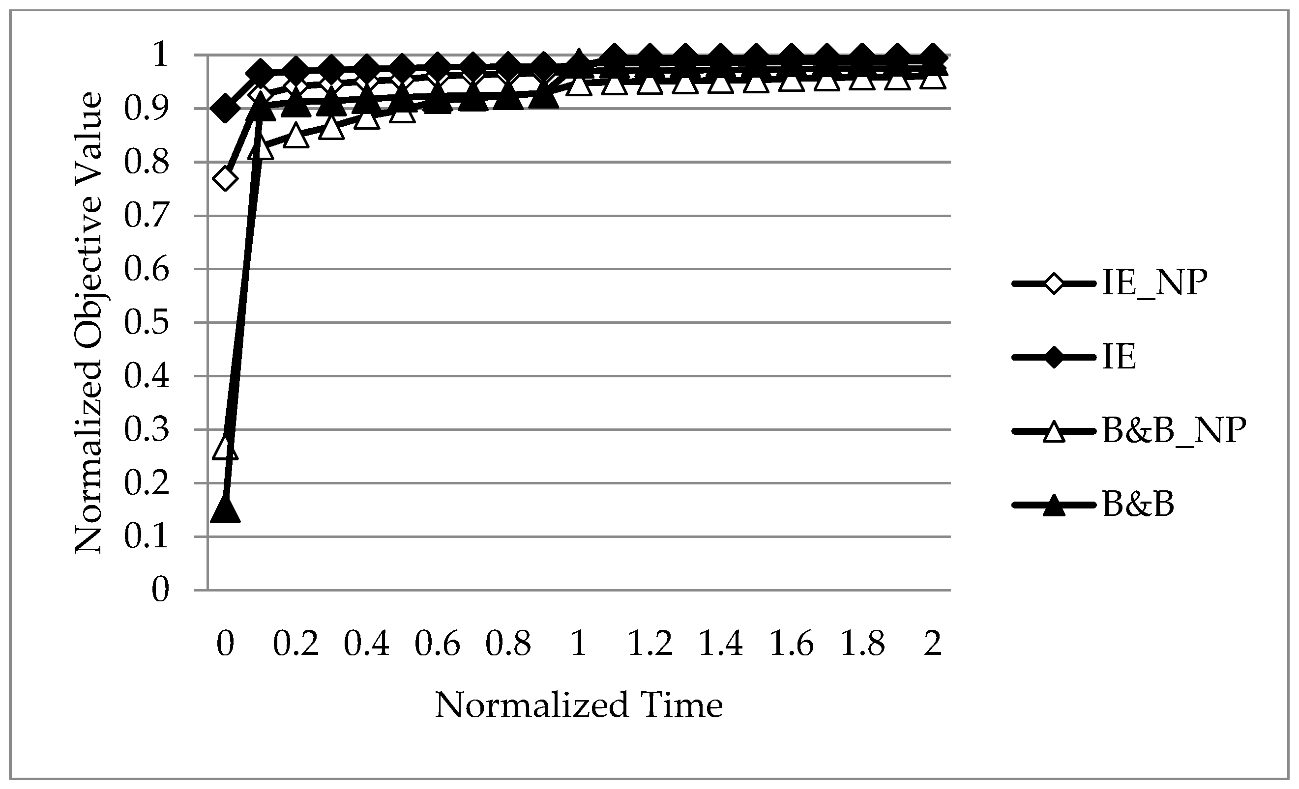
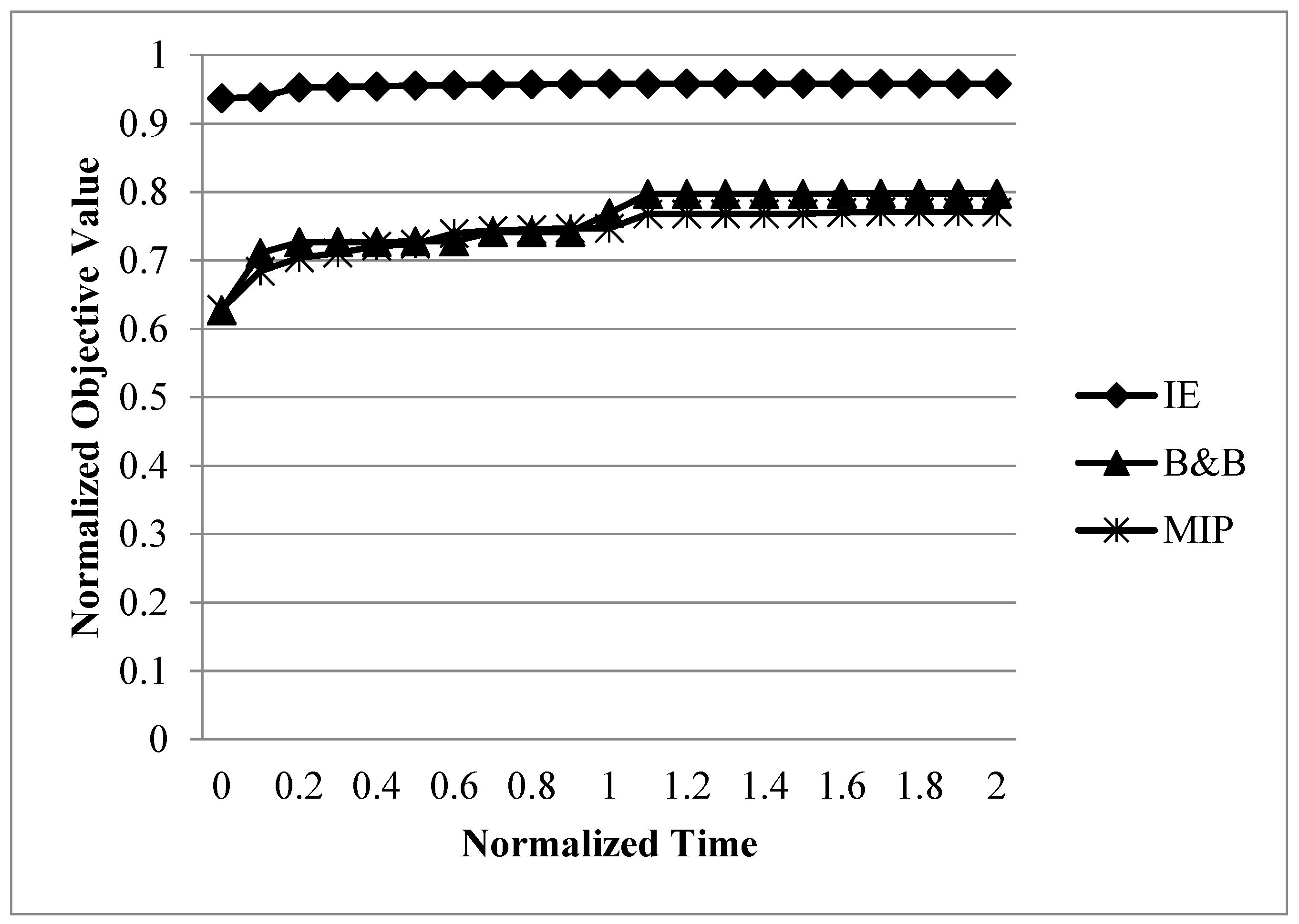
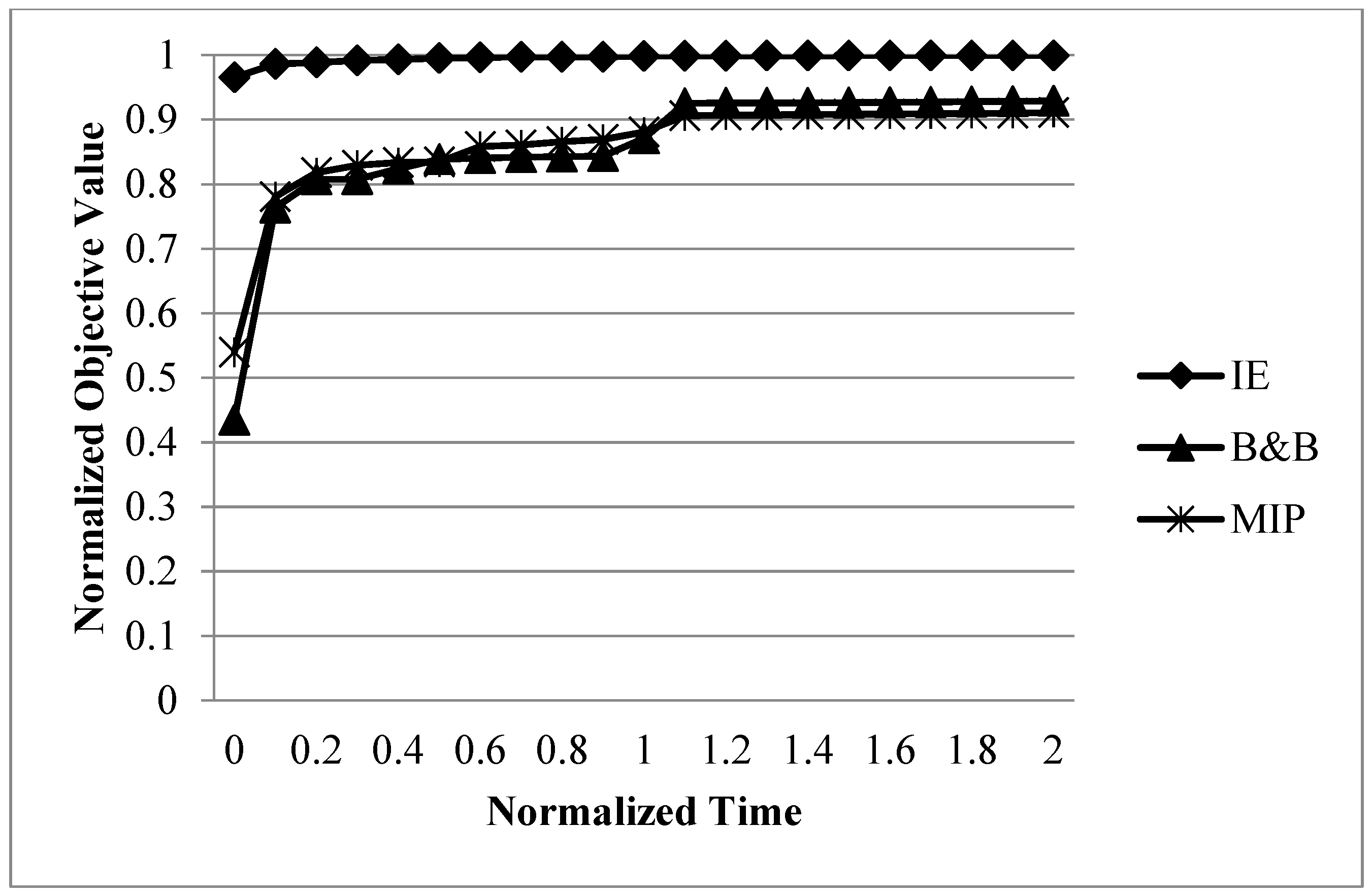
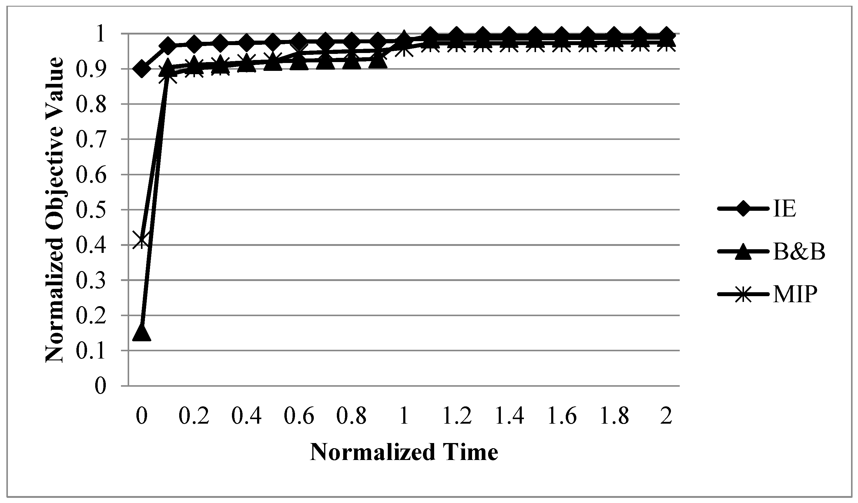
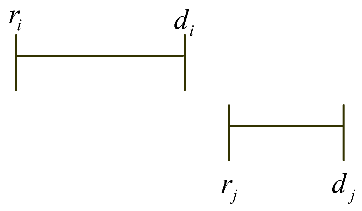
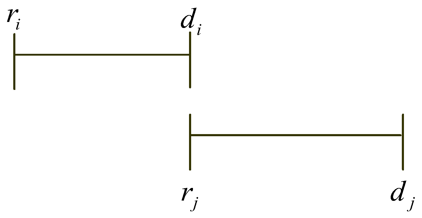
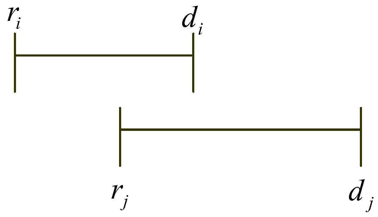
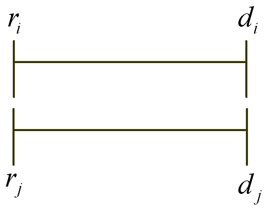
To solve the TMP optimally using problem-specific structural properties, an IE method is developed. Unlike the MIP model, which relies on a general-purpose solver, the IE method explicitly explores the solution space by constructing feasible job sequences. Each node in the enumeration tree represents a partial sequence of selected jobs, and the method systematically extends these sequences while checking feasibility with respect to time window constraints. This framework serves as the basis for incorporating additional techniques, including midpoint-based ordering for guiding the search and dominance rules derived from the partial ordering (⇒) to prune the search tree, thereby improving computational efficiency.

This section presents an IE procedure using a depth-first search (DFS) scheme to identify an optimal solution. Let $l$ denote the level in the enumeration tree. A node at level $l$ represents a partial solution consisting of $l$ scheduled jobs. The sequence of these $l$ jobs is defined by the path from the root node to the current node. By appending a not-yet-selected job to the current partial solution, a new sequence is generated, which corresponds to a child node at level $l$ + 1 in the tree.

Suppose there are $n$ jobs in a TMP instance. The root node at level 0 represents an empty solution with no selected jobs. From the root, $n$ branches can be created, each corresponding to the selection of one of the $n$ jobs, leading to child nodes at level 1. In general, a node at level $l$ branches into $n-l$ child nodes at level $l+1$, each representing the addition of a not-yet-selected job. Therefore, the number of nodes at level $l$ is given by the permutation $P_l^n$ = ${\displaystyle \frac{n!}{\left(n-l\right)!}}$ = $n\times \left(n-1\right)\times \dots \times (n-l+1)$. At the bottom level (level $n$), there are $n!$ nodes, each representing a complete sequence of all $n$ jobs. Consequently, the total number of nodes in a complete enumeration tree is: $P_0^n+P_1^n+\cdots +P_{n-1}^n+P_n^n$.

By developing heuristic sorting, dominance rules, and an LP relaxation of subproblems, each discussed in detail below, this study effectively reduces the number of nodes generated in the enumeration tree, thereby significantly decreasing computation time.

Let $H$ denote the solution associated with the current node in the enumeration tree. Let $\omega \left(H\right)$ represent the set of jobs included in $H$, $\lambda \left(H\right)$ denote the last job in $H$, and $C_{\lambda \left(H\right)}^E$ be the earliest completion time of job $\lambda \left(H\right)$. The notation $H+j$ refers to the solution obtained by appending a job $j\in J-\omega \left(H\right)$ immediately after the last job in $H$.

Let $P\left\{\tau \right|J\}$ denote a TMP instance in which the set of considered jobs $J$ can only be scheduled after time $\tau$. Let $P^{\ast }\left\{\tau \right|J\}$ be an optimal solution to $P\left\{\tau \right|J\}$, and let $O^{\ast }\left\{\tau \right|J\}$ denote the corresponding optimal objective value of $P^{\ast }\left\{\tau \right|J\}$.

Lemma 1.

For a given job set $J$ and two time points ${\tau }_1$ and ${\tau }_2$ , consider the problems $P\left\{{\tau }_1\right|J\}$ and $P\left\{{\tau }_2\right|J\}$, with corresponding optimal objective values $O^{\ast }\left\{{\tau }_1\right|J\}$ and $O^{\ast }\left\{{\tau }_2\right|J\}$, respectively. If ${\tau }_1<{\tau }_2$, then $O^{\ast }\left\{{\tau }_1\right|J\}\ge O^{\ast }\{{\tau }_2\left|J\right\}$.

Proof. 

Since ${\tau }_1\le {\tau }_2$ and the set of selectable jobs is identical for the two problems, any optimal solution of $P\left\{{\tau }_2|J\right\}$ is also feasible for $P\left\{{\tau }_1|J\right\}$. In a maximization problem, the objective value of a feasible solution cannot exceed that of an optimal solution. Therefore, the objective value of a feasible solution in a maximization problem is less than or equal to that of an optimal one. Therefore, $O^{\ast }\left\{{\tau }_1\right|J\}\ge O^{\ast }\{{\tau }_2\left|J\right\}$. □

Lemma 1 indicates that an earlier available starting time provides greater flexibility for scheduling jobs, and therefore cannot lead to a worse optimal objective value under the same job set.

Lemma 2.

For a fixed time $\tau$ and two job sets $J_1$ and $J_2$, consider the problems $P\left\{\tau \right|J_1\}$ and $P\left\{\tau \right|J_2\}$, with corresponding optimal objective values $O^{\ast }\left\{\tau \right|J_1\}$ and $O^{\ast }\left\{\tau \right|J_2\}$, respectively. If $J_1\supset J_2$, then $O^{\ast }\left\{\tau \right|J_1\}\ge O^{\ast }\{\tau \left|J_2\right\}$.

Proof. 

Since $J_1\supset J_2$ and the time horizon is identical for both problems, any optimal solution of $P\left\{\tau |J_2\right\}$ is also feasible for $P\left\{\tau |J_1\right\}$. In a maximization problem, the objective value of a feasible solution cannot exceed that of an optimal solution. Therefore, $O^{\ast }\left\{\tau \right|J_1\}\ge O^{\ast }\{\tau \left|J_2\right\}$. □

Lemma 2 indicates that enlarging the set of available jobs cannot reduce the optimal objective value. With more candidate jobs to choose from, the decision maker has greater flexibility, and therefore the optimal objective value cannot be worse than that obtained from a subset of jobs. Together, Lemmas 1 and 2 show that increasing scheduling flexibility, either through earlier start times or larger job sets, cannot reduce the optimal objective value.

Based on the assumption that a selected job must be fully processed within its time window, Dominance Rule 1 follows directly.

Dominance rule 1. Consider the subproblem $P\left\{C_{\lambda \left(H\right)}^E\right|J-\omega \left(H\right)\}$ For any job $j\in J-\omega \left(H\right)$, if $\max \left(r_j,C_{\lambda \left(H\right)}^E\right)+p_j>d_j$, then the child node $H+j$ can be fathomed. □

This rule eliminates jobs that cannot be feasibly scheduled after the current partial sequence. If the earliest possible start time of job $j$, given by $\max \left(r_j,C_{\lambda \left(H\right)}^E\right)$, already leads to a completion time beyond its due date, then job $j$ cannot be included in any feasible extension of the current solution. Therefore, such nodes can be safely pruned without losing optimality.

4.3.1. Methods Based on Ordering Relations

This subsection utilizes two ordering relations: a partial ordering $\Rightarrow$ for deriving dominance rules, and a midpoint-based ordering $\to$ for guiding job sequencing.

Definition 1.

(Relation operator ⇒) For two jobs $i,j\in J$, the relation $i\Rightarrow j$ holds if and only if $r_i\le r_j$ and $d_i\le d_j$.

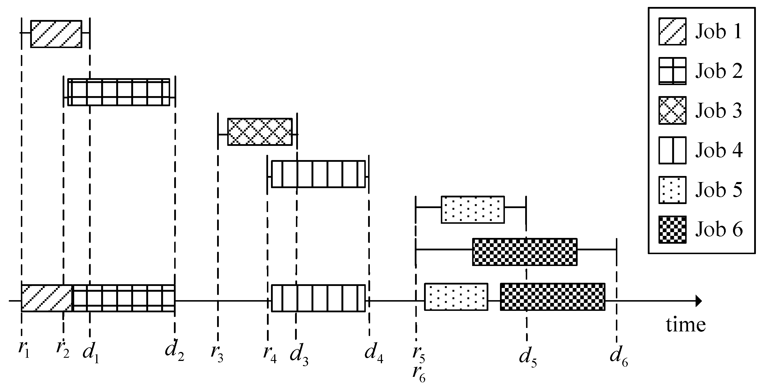
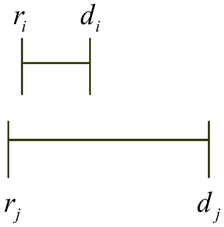
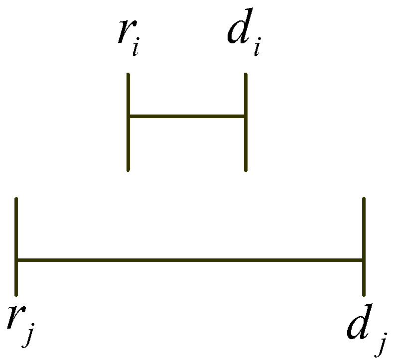
According to this definition, jobs $i$ $\Rightarrow$ $j$ means that the time window of job $i$ is no later than that of job $j$; that is, both the ready date and the due date of job $i$ are less than or equal to those of job $j$.

Definition 2.

(Equivalence under relation ⇒) For two jobs $i,j\in J$, they are considered equivalent under the relation $\Rightarrow$ if and only if $r_i=r_j$ and $d_i=d_j$.

This definition identifies jobs with identical time windows. Such jobs are indistinguishable with respect to the relation $\Rightarrow$, and therefore can be treated equivalently when sorting the job set. Such jobs have identical scheduling flexibility and do not impose any ordering preference under the relation $\Rightarrow$.

Definition 3.

(Equivalence notation ⇔) If two jobs $i,j\in J$ are equivalent under the relation $\Rightarrow$, they are denoted as $i\iff j$.

Lemma 3.

For any two jobs $i,j\in J$, the relation $i\iff j$ holds if and only if both $i\Rightarrow j$ and $j\Rightarrow i$.

Proof. 

(if) Suppose $i\Rightarrow j$ and $j\Rightarrow i$, then $r_i\le r_j$, $d_i\le d_j$, $r_j\le r_i$, and $d_j\le d_i$. Hence, we have $r_i=r_j$ and $d_i=d_j$, which implies jobs $i$ and $j$ are equivalent under $\Rightarrow$, i.e., $i\iff j$.

• (only if) If $i\iff j$, then by Definition 2, $r_i=r_j$ and $d_i=d_j$. Therefore, both $i\Rightarrow j$ and $j\Rightarrow i$ hold. □

This lemma shows that the equivalence relation $\iff$ corresponds to a mutual relation under $\mathit{\Rightarrow }$.

Lemma 4.

The relation $\Rightarrow$ defined on the set $J$ is a partial ordering.

Proof. 

A partial ordering has to satisfy reflexivity, transitivity, and antisymmetry. reflexivity: For any job $i\in J$, since $r_i\le r_i$ and $d_i\le d_i$, we have $i\Rightarrow i$. transitivity: For any jobs $i, j, k\in J$, if $i\Rightarrow j$ and $j\Rightarrow k$, then $r_i\le r_j\le r_k$ and $d_i\le d_j\le d_k$. Hence, $r_i\le r_k$ and $d_i\le d_k$, which implies $i\Rightarrow k$. anti-symmetry: For any jobs $i, j\in J$, if $i\Rightarrow j$ and $j\Rightarrow i$, then $r_i=r_j$ and $d_i=d_j$. Therefore, $i$ and $j$ are equivalent under $\Rightarrow$; i.e., $i\iff j$. □

The job set $J$, together with the relation $\Rightarrow$, forms a partially ordered set (or poset) denoted as $(J,\Rightarrow )$. Two jobs $i,j\in J$ are called incomparable if neither $i\Rightarrow j$ nor $j\Rightarrow i$ holds. This occurs when one job has an earlier ready date but a later due date than the other, i.e., when ($r_i\le r_j$ and $d_i\ge d_j$) or ($r_i\ge r_j$ and $d_i\le d_j$). In such cases, neither job dominates the other under this relation. A poset becomes a total ordering if no pair of elements is incomparable. However, in the problem considered in this study, incomparable job pairs may exist. Therefore, the poset $(J,\Rightarrow )$ is not a total ordering. This partial ordering is used to support the development of dominance rules.

Definition 4.

(Relation operator →) For two jobs $i,j\in J$, the relation $i\to j$ holds if and only if $r_i+d_i\le r_j+d_j$.

This condition is equivalent to comparing the midpoints of the time windows. Specifically, it implies that ${\displaystyle \frac{r_i+d_i}{2}}\le {\displaystyle \frac{r_j+d_j}{2}}$, i.e., the midpoint of the time window of job $i$ is less than or equal to that of job $j$.

Definition 5.

(Equivalence under relation →) Two jobs $i,j\in J$ are considered equivalent under the relation $\to$ if and only if $r_i+d_i=r_j+d_j$.

This condition is equivalent to ${\displaystyle \frac{r_i+d_i}{2}}={\displaystyle \frac{r_j+d_j}{2}}$, i.e., the midpoints of the time windows of jobs $i$ and $j$ are identical. Such jobs are indistinguishable under the ordering defined by $\to$ and may be treated equivalently during sorting.

Definition 6.

(Equivalence notation ↔) If two jobs $i,j\in J$ are equivalent under the relation $\to$, they are denoted by $i\leftrightarrow j$.

This notation indicates that the two jobs have identical midpoint values of their time windows.

Lemma 5.

For two jobs $i,j\in J$, the relation $i\leftrightarrow j$ holds if and only if both $i\to j$ and $j\to i$ hold.

Proof. 

(if) Suppose $i\leftrightarrow j$. Then, by Definition 5, $r_i+d_i=r_j+d_j$. This implies $r_i+d_i\le r_j+d_j$ and $r_j+d_j\le r_i+d_i$, and therefore both $i\to j$ and $j\to i$ hold.

• (only if) Suppose $i\to j$ and $j\to i$. Then $r_i+d_i\le r_j+d_j$ and $r_j+d_j\le r_i+d_i$. These two inequalities imply $r_i+d_i=r_j+d_j$. Hence, $i\leftrightarrow j$. □

This lemma shows that equivalence under $\to$ corresponds to mutual ordering based on midpoint comparison.

Lemma 6.

The relation $\to$ defined on the set $J$ is a total preorder.

Proof. 

The relation $\to$ satisfies the following properties: Reflexivity: For any job $i\in J$, $r_i+d_i\le r_i+d_i$, hence $i\to i$. Transitivity: For jobs $i, j, k\in J$, if $i\to j$ and $j\to k$, then $r_i+d_i\le r_j+d_j$ and $r_j+d_j\le r_k+d_k$. Adding these two inequalities yields $r_i+d_i\le r_k+d_k$, which implies $i\to k$. Totality: For any two jobs $i, j\in J$, either $r_i+d_i\le r_j+d_j$ or $r_j+d_j\le r_i+d_i$, hence either $i\to j$ or $j\to i$ (or both). □

The job set $J$, together with the relation $\to$, forms a totally preordered set. Two jobs may be equivalent under this relation if they share the same midpoint. By grouping equivalent jobs into equivalence classes, the induced ordering among these classes becomes a total ordering.

Lemma 7.

For any two jobs $i,j\in J$, if $i\Rightarrow j$, then $i\to j$.

Proof. 

Since $i\Rightarrow j$, we have $r_i\le r_j$ and $d_i\le d_j$. Adding these two inequalities yields $r_i+d_i\le r_j+d_j$. Therefore, $i\to j$. □

This lemma shows that the partial ordering $\Rightarrow$ is consistent with the midpoint-based ordering $\to$.

Lemma 8.

Suppose two jobs $i,j\in J$ satisfy $i\leftrightarrow j$. Then, for any job $k\in J-\{i,j\}$, the following two statements hold.

(1)

If $k\to i$, then $k\to j$.

(2)

If $i\to k$, then $j\to k$.

Proof. 

Since $i\leftrightarrow j,$ we have $r_i+d_i=r_j+d_j$.

(1)

If $k\to i$, then we have $r_k+d_k\le r_i+d_i$.

Substituting $r_j+d_j$ for $r_i+d_i$, we obtain $r_k+d_k\le r_j+d_j$, which implies $k\to j$.

(2)

If $i\to k$, then we have $r_i+d_i\le r_k+d_k$.

Substituting $r_j+d_j$ for $r_i+d_i$, we obtain $r_j+d_j\le r_k+d_k$, which implies $j\to k$. □

This lemma shows that jobs with identical midpoints are interchangeable under the relation $\to$.

Lemma 9.

If no pair of jobs in $J$ satisfies the equivalence relation $\leftrightarrow$, then there exists a unique sequence of jobs sorted by the relation $\to$. Furthermore, if there exists a subset $J^s\subset J$ such that every pair of jobs in $J^s$ satisfies the relation $\leftrightarrow$, then the jobs in $J^s$ appear consecutively as a group in the sequence sorted by $\to$.

Proof. 

The result follows from Lemma 8 and the transitivity and totality properties of the relation $\to$. If no pair of jobs is equivalent under $\leftrightarrow$, then all jobs are strictly ordered by their midpoint values, yielding a unique sorted sequence. If a subset $J^s$ consists of jobs equivalent under $\leftrightarrow$, then by Lemma 8 these jobs are interchangeable under the relation $\to$, and therefore they must appear consecutively in any sequence sorted by $\to$. □

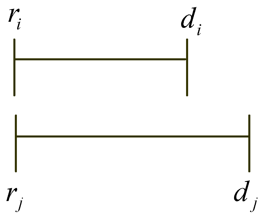
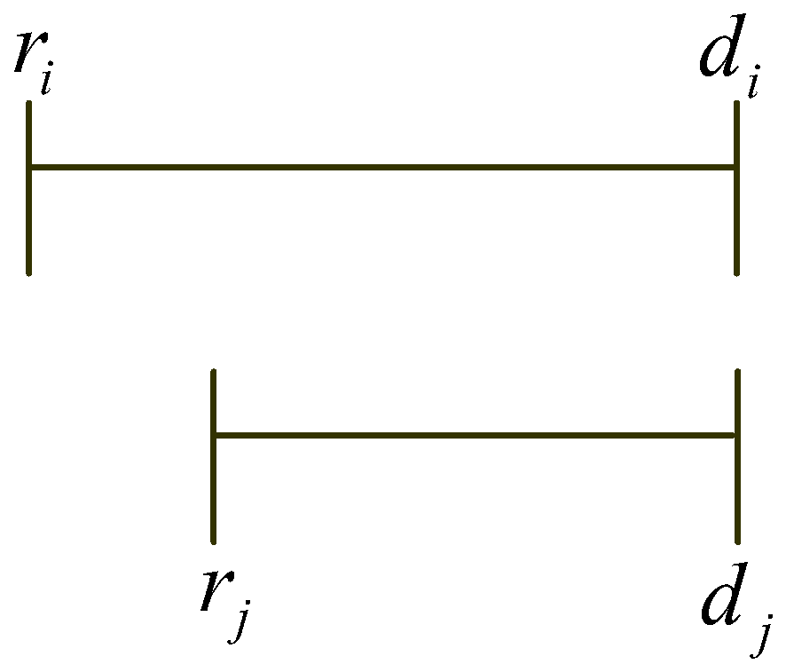
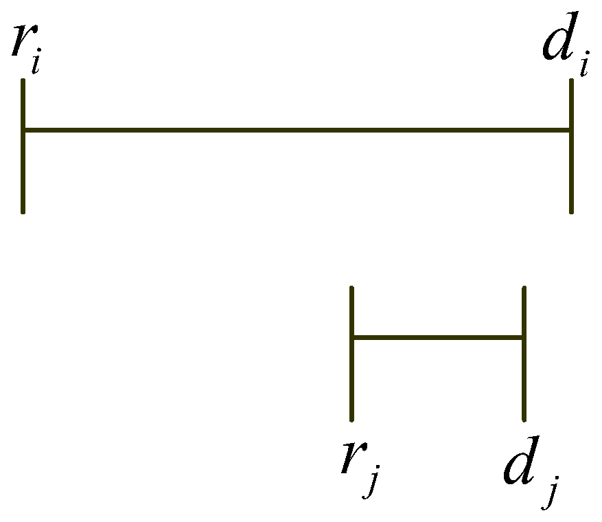
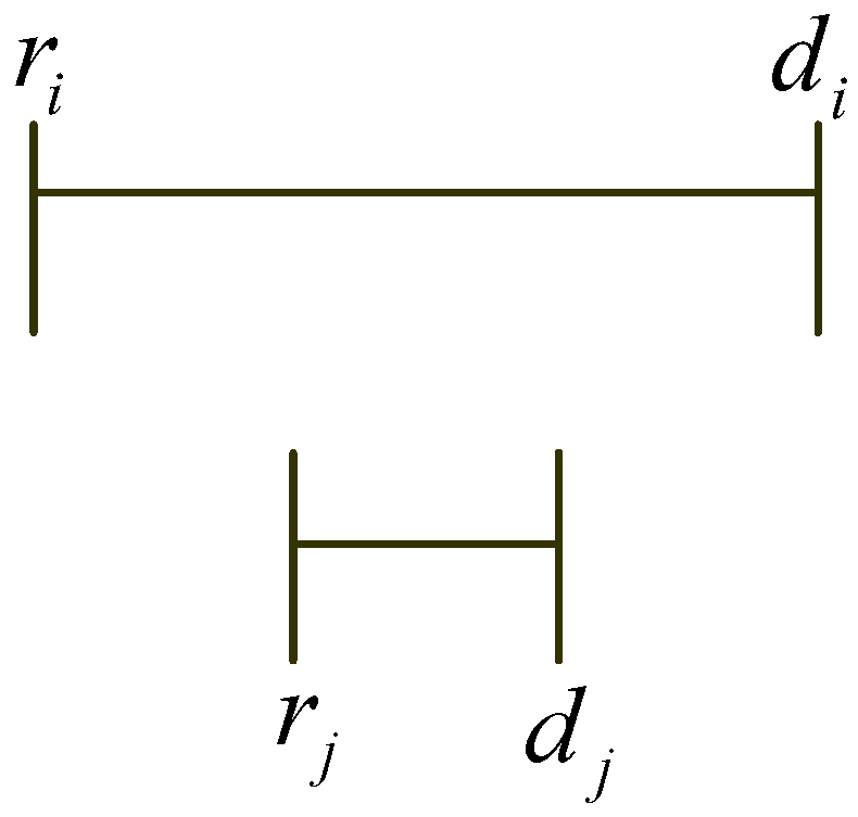
Under the condition that two jobs $i,j\in J$ satisfy $i\to j$, there are ten possible cases for the relationships among $r_i$, $d_i$, $r_j$, and $d_j$. These cases are detailed in Appendix A. Among them, Cases 1 through 6 also satisfy $i\Rightarrow j$, with Case 4 further satisfying $i\iff j$. In addition, Cases 8 and 10 satisfy the equivalence condition $i\leftrightarrow j$.

Lemma 10.

If $i\to j$ and ($r_i\ne r_j$ or $d_i\ne d_j$), then $j\Rightarrow i$ cannot hold.

Proof. 

Assume $i\to j$. Then $r_i+d_i\le r_j+d_j$. Suppose, for contradiction, $j\Rightarrow i$ holds. Then, $r_j\le r_i$ and $d_j\le d_i$. Adding these inequalities gives $r_j+d_j\le r_i+d_i$. Combining this with $r_i+d_i\le r_j+d_j$, we obtain $r_i+d_i=r_j+d_j$.

Since $r_j\le r_i$ and $d_j\le d_i$, if either inequality were strict, then $r_j+d_j<r_i+d_i$, which is impossible. Therefore, $r_j=r_i$ and $d_j=d_i$. This contradicts the assumption that $r_i\ne r_j$ or $d_i\ne d_j$. Therefore, $j\Rightarrow i$ cannot hold. □

This lemma indicates that a strict ordering under the midpoint-based relation $\to$ prevents a reverse dominance relationship under $\Rightarrow$.

Lemma 11.

Consider two jobs $i,j\in J$ such that $i\Rightarrow j$ and $r_j<d_i$. Suppose $H^{ji}$ is an optimal schedule in which job $i$ is scheduled immediately after job $j$ . Then, there exists a feasible schedule $H^{ij}$ obtained by exchanging the positions of $i$ and $j$, while keeping the positions of all other jobs in $H^{ji}$ unchanged. Moreover, $H^{ij}$ is also optimal.

Proof. 

Let $S_j^{ji}$, $C_j^{ji}$ and $S_i^{ji}$, $C_i^{ji}$ denote the start and completion times of jobs $j$ and $i$, respectively, in schedule $H^{ji}$. Let $S_j^{ij}$, $C_j^{ij}$ and $S_i^{ij}$, $C_i^{ij}$ denote the start and completion times of jobs $j$ and $i$, respectively, in schedule $H^{ij}$. Since $H^{ji}$ is feasible, $r_j\le S_j^{ji}$, $r_i\le S_i^{ji}$, $C_j^{ji}\le d_j$, and $C_i^{ji}\le d_i$. Construct schedule $H^{ij}$ by swapping the positions of jobs $i$ and $j$. Then, $S_i^{ij}=S_j^{ji}$, $C_j^{ij}=C_i^{ji}$.

(1)

Feasibility of job $i$: Since $S_i^{ij}$ = $S_j^{ji}$ and $r_j\le S_j^{ji}$, we have $r_j\le S_i^{ij}$. Because $i\Rightarrow j$, we have $r_i\le r_j$, hence $r_i\le S_i^{ij}$. Also, since job $i$ is scheduled before job $j$ in $H^{ij}$, its completion time satisfies $C_i^{ij}\le C_i^{ji}\le d_i$. Thus, job $i$ remains feasible.

(2)

Feasibility of job $j$: Since $C_j^{ij}=C_i^{ji}\le d_i$ and $i\Rightarrow j$ implies $d_i\le d_j$, we have $C_j^{ij}\le d_j$. Also, because job $j$ is scheduled after job $i$, its start time satisfies $S_j^{ij}\ge S_i^{ij}=S_j^{ji}\ge r_j$. Thus, job $j$ remains feasible.

(3)

Optimality: Since the set of selected jobs remains unchanged, the objective value is unchanged. Therefore, $H^{ij}$ is also an optimal schedule. □

This lemma shows that when job $i$ is no later and no looser than job $j$, scheduling $i$ before $j$ is always at least as good as the reverse order.

Lemma 12.

If two jobs $i$ and $j$ satisfy $i\Rightarrow j$, then any schedule in which job $i$ is scheduled immediately after job $j$ cannot be a unique optimal schedule.

Proof. 

Consider two cases.

• $d_i\le r_j$: In this case, the time window $\left[r_i, d_i\right]$ of job $i$ lies entirely before $\left[r_j, d_j\right]$. Therefore, it is impossible to schedule job $j$ before job $i$. Hence, any schedule in which job $i$ is scheduled immediately after job $j$ is infeasible.
• $d_i>r_j$: In this case, the time windows overlap. By Lemma 11, any optimal schedule in which job $i$ is scheduled immediately after job $j$ can be transformed into another optimal schedule by exchanging the position of $i$ and $j$. Therefore, such a schedule cannot be unique. □

Therefore, when $i\Rightarrow j$, it is unnecessary to consider any schedule in which job $i$ is scheduled immediately after $j$. Following Lemma 12, we establish the following dominance rule:

Dominance rule 2. If two jobs $i$ and $j$ satisfy $i\Rightarrow j$, then any child node obtained by scheduling job $i$ immediately after job $\mathrm{j}$ in the current partial solution can be fathomed. □

This rule follows from Lemma 12, since any such node either corresponds to an infeasible schedule or can be transformed into another node with an equivalent or better solution by exchanging the positions of jobs $i$ and $j$.

Lemma 13.

If every pair of jobs in $J$ is comparable under the relation $\Rightarrow$, then there exists an optimal solution in which the sequence of selected jobs follows the nondecreasing order defined by $\Rightarrow$. Consequently, given this sorted order, at any node representing a selected job, it is sufficient to branch only to jobs that appear later in the sequence.

Proof. 

Since every pair of jobs is comparable under $\Rightarrow$, the relation defines a total ordering on $J$. Consider any optimal solution. If the sequence of selected jobs violates this ordering, then there exists at least one adjacent pair of jobs $j$, $i$ such that $i\Rightarrow j$ but $j$ is scheduled before $i$. By Lemma 11, such a pair can be exchanged without violating feasibility or optimality. Repeatedly applying such exchanges transforms the sequence into one that follows the order defined by $\Rightarrow$ without changing the objective value. Hence, there exists an optimal solution consistent with the sorted order.

Therefore, when constructing solutions, it is sufficient to branch only to jobs that appear later in the sorted sequence. □

This lemma shows that, under a total ordering, the search space can be restricted to sequences consistent with the ordering without loss of optimality.

4.3.2. Heuristic Sorting of Jobs

As discussed in Lemma 13 and Dominance Rule 2, the relation $\Rightarrow$ offers a strong structural property for sequencing jobs when searching for an optimal solution. Specifically, if $i\Rightarrow j$, it is only necessary to consider scheduling job $j$ after job $i$, rather than the reverse. However, the poset $(J,\Rightarrow )$ is not a total ordering; that is, not all pairs of jobs can be compared by $\Rightarrow$. As a result, it may not be possible to derive a complete sorting of all jobs based solely on $\Rightarrow$. In contrast, the relation $\to$ provides a complete ordering of jobs based on the midpoints of their time windows. Therefore, the relation $\Rightarrow$ is used for dominance-based pruning, while the relation $\to$ is used for heuristic ordering.

According to Lemma 10, sorting by $\to$ does not contradict the ordering defined by $\Rightarrow$ when a job pair is comparable under $\Rightarrow$. Among the ten possible cases describing the relationship between jobs $i$ and $j$ where $i\to j$ holds, six cases (Cases 1 through 6) also satisfy $i\Rightarrow j$. For these six cases, it is unnecessary to consider solutions in which job $i$ is scheduled immediately after job $j$.

For a job pair $i$ and $j$ that satisfies $i\to j$ but not $i\Rightarrow j$, scheduling job $i$ before job $j$ is not guaranteed to yield an optimal solution. However, the relation $i\to j$ implies that $d_j-r_i\ge d_i-r_j$, which indicates that the interval $[r_i,d_j]$ (corresponding to scheduling job $i$ before job $j$) is wider than the interval $[r_j,d_i]$ (which results from scheduling job $j$ before job $i$). Therefore, when both jobs are selected under the condition $i\to j$, scheduling $i$ before $j$ provides more slack and flexibility than the reverse order. Consequently, sorting jobs according to the relation $\to$ offers a useful heuristic for guiding the search process.

Moreover, since a depth-first search (DFS) strategy is employed in the enumeration tree, following the branching sequence defined by the sorted list increases the likelihood of generating a high-quality solution early. If the first solution generated by the sorted sequence is feasible and not eliminated by any dominance rule, it serves as a strong initial incumbent solution in the search for optimality.

4.3.3. Additional Dominance Rules

In addition to the dominance rules presented in the previous subsection, this subsection introduces further rules to reduce branching in the enumerative search tree. These additional rules exploit the structural properties of the scheduling problem and the ordering relations defined in this study to identify and eliminate dominated or redundant branches during the search process.

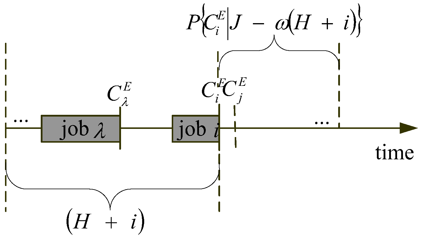
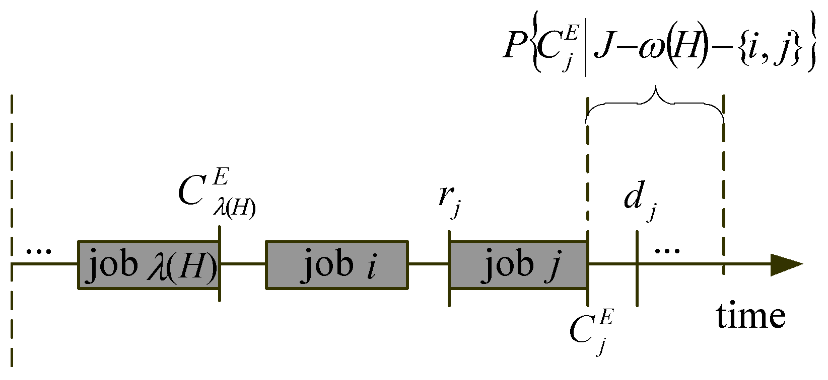
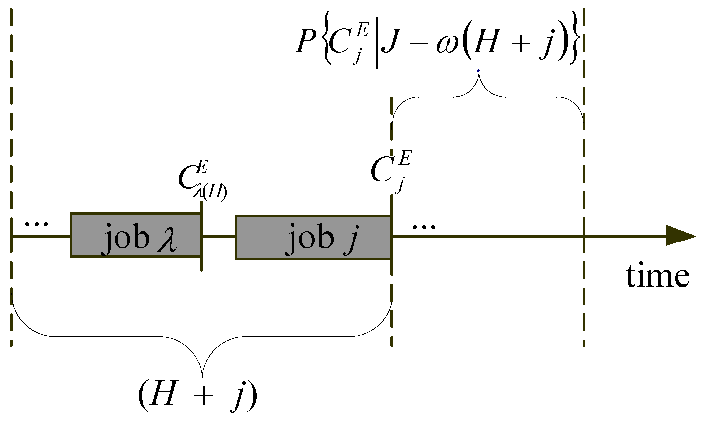
Figure 3 illustrates that job $i$ can be inserted between the last scheduled job in $H$ and job $j$ without delaying the earliest completion time of job j, denoted by $C_j^E$.

Lemma 14.

Given a partial solution $H$, consider the subproblem $P\left\{C_{\lambda \left(H\right)}^E\right|J-\omega \left(H\right)\}$. If there exist two jobs $i,j\in J-\omega \left(H\right)$ such that $\min \left(d_i,r_j\right)-\mathrm{m}\mathrm{a}\mathrm{x}(C_{\lambda \left(H\right)}^E,r_i)\ge p_i$, then the following inequality holds: $w_j+O^{\ast }\left\{C_j^E|J-\omega \left(H+j\right)\right\}\le w_i+w_j+O^{\ast }\left\{C_j^E\right|J-\omega (H+i+j)\}$.

Proof. 

The condition implies that job $i$ can be inserted between the last scheduled job in $H$ and job $j$ without delaying the earliest completion time of job $j$, denoted by $C_{\lambda \left(H\right)}^E$ (see Figure 3). Consider two cases.

• Job $i$ is selected in an optimal solution of $P\left\{C_j^E|J-\omega (H+j)\right\}$. In this case, job $i$ is originally scheduled after job $j$ without affecting $C_j^E$, we can exchange its position to occur before $j$. This increases the total weight accumulated before $C_j^E$ by $w_i$, while potentially creating additional space after $C_j^E$ for other jobs. Therefore, $O^{\ast }\left\{C_j^E|J-\omega (H+j)\right\}\le O^{\ast }\left\{C_j^E|J-\omega (H+i+j)\right\}$.
• Suppose job $i$ is not selected in the optimal solution of $P\left\{C_j^E|J-\omega (H+j)\right\}$. Since job $i$ can be inserted before job $j$ without affecting $C_j^E$, including $i$ does not reduce the optimal value. Therefore, $O^{\ast }\left\{C_j^E|J-\omega \left(H+j\right)\right\}=O^{\ast }\left\{C_j^E\right|J-\omega (H+i+j)\}$

Combining both cases and noting that $w_j\le w_i+w_j$, we obtain $w_j+O^{\ast }\left\{C_j^E|J-\omega (H+j)\right\}\le w_i+w_j+O^{\ast }\left\{C_j^E|J-\omega (H+i+j)\right\}$. □

This lemma shows that inserting job $i$ before job $j$, when feasible without delaying the earliest completion time of job $j$, cannot worsen the objective value and may improve it.

Dominance rule 3. Consider a subproblem $P\left\{C_{\lambda \left(H\right)}^E\right|J-\omega \left(H\right)\}$ of a partial solution $H$. If there exist two jobs $i,j\in J-\omega \left(H\right)$ such that $\min \left(d_i,r_j\right)-\mathrm{m}\mathrm{a}\mathrm{x}(C_{\lambda \left(H\right)}^E,r_i)\ge p_i$, then the child node corresponding to the partial schedule $H+j$ can be fathomed. □

This rule follows from Lemma 14. Since inserting job $i$ before job $j$ does not delay the earliest completion time of job $j$ and yields a solution that is at least as good as (and potentially better than) scheduling $j$ immediately after $H$. Thus, branching directly from $H$ to $H+j$ can be skipped.

Lemma 15.

Consider a subproblem $P\left\{C_{\lambda \left(H\right)}^E\right|J-\omega \left(H\right)\}$ of a partial solution $H$. If there exist two jobs $i,j\in J-\omega \left(H\right)$ such that $\left[\max \left(C_{\lambda \left(H\right)}^E,r_j\right)+p_j\right]+p_i>d_i$, $\left[\max \left(C_{\lambda \left(H\right)}^E,r_i\right)+p_i\right]+p_j>d_j$, $w_i\ge w_j$, and $\max \left(C_{\lambda \left(H\right)}^E,r_i\right)+p_i\le \max \left(C_{\lambda \left(H\right)}^E,r_j\right)+p_j$, then the following inequality holds: $w_i+O^{\ast }\left\{C_i^E\right|J-\omega (H+i)\}\ge w_j+O^{\ast }\{C_j^E|J-\omega (H+j\left)\right\}$.

Proof. 

The two cases of adding job $i$ or job $j$ after $H$ are illustrated in Figure 4 and Figure 5, respectively.

The first two conditions imply mutual exclusion:

• If job $j$ is scheduled immediately after $H$, then job $i$ cannot be scheduled afterward.
• Similarly, if job $i$ is scheduled after $H$, then job $j$ cannot be scheduled afterward.

Thus, for both subproblems $P\left\{C_j^E|J-\omega (H+j)\right\}$ and $P\left\{C_i^E|J-\omega (H+i)\right\}$, the remaining job set is identical and equals $J-\omega \left(H\right)-\left\{i, j\right\}$. Let $C_i^E=\mathrm{m}\mathrm{a}\mathrm{x}\left(C_{\lambda \left(H\right)}^E,r_i\right)+p_i$, $C_j^E=\mathrm{m}\mathrm{a}\mathrm{x}\left(C_{\lambda \left(H\right)}^E,r_j\right)+p_j$. By assumption, $C_i^E\le C_j^E$. By Lemma 1, this implies $O^{\ast }\left\{C_i^E|J-\omega (H+i)\right\}\ge O^{\ast }\left\{C_j^E|J-\omega (H+j)\right\}$. Since $w_i\ge w_j$, we obtain $w_i+O^{\ast }\left\{C_i^E|J-\omega (H+i)\right\}\ge w_j+O^{\ast }\left\{C_j^E|J-\omega (H+j)\right\}$. □

This lemma shows that when selecting one job that excludes the other, the job with the earlier completion time and no smaller weight dominates the alternative.

Following Lemma 15, we have Dominance rule 4. This rule follows from Lemma 15, since selecting job $i$ excludes job $j$, and job $i$ yields an objective value that is at least as good as that obtained by selecting job $j$.

Dominance rule 4. Consider a node representing solution $H$ and its subproblem $P\left\{C_{\lambda \left(H\right)}^E\right|J-\omega \left(H\right)\}$. If there exist two jobs $i,j\in J-\omega \left(H\right)$ such that $w_i\ge w_j$, $\left[\max \left(C_{\lambda \left(H\right)}^E,r_j\right)+p_j\right]+p_i>d_i$, $\left[\max \left(C_{\lambda \left(H\right)}^E,r_i\right)+p_i\right]+p_j>d_j$, and $\max \left(C_{\lambda \left(H\right)}^E,r_i\right)+p_i\le \max \left(C_{\lambda \left(H\right)}^E,r_j\right)+p_j$, then the child node corresponding to solution $H+j$ can be fathomed. □

If only one of the two jobs $i$ and $j$ can be scheduled after partial solution $H$ due to timing constraints, and job $i$ has a weight no smaller than that of job $j$, and completes no later than job $j$, then selecting job $i$ dominates selecting job $j$. Therefore, branching to $H+j$ is unnecessary. That is, any solution obtained from node $H+j$ cannot outperform a corresponding solution obtained from node $H+i$.

4.3.4. Implementation of the Enumerative Method

With the proposed dominance rules and heuristic job sorting, the enumerative method is implemented using a depth-first search (DFS) strategy. At each node, candidate jobs are explored according to the ordering defined by the relation $\to$, while the dominance rules are applied to prune infeasible or dominated branches.

The DFS strategy requires minimal memory, since only the nodes along the current path from the root to the active partial solution need to be stored. The search procedure is implemented as a recursive function, which is outlined in Appendix B.

4.4. B&B Method with LP-Relaxation

The B&B scheme presented in this section differs from the general-purpose framework used by Gurobi to solve the MIP model. In the proposed approach, each node in the branching tree represents a partial sequence of selected jobs, and branching corresponds to extending this sequence by selecting an additional eligible job. In contrast, Gurobi operates on the MIP formulation and explores nodes defined by restrictions on decision variables. Therefore, the proposed B&B method is a problem-specific enumeration scheme rather than the generic B&B procedure used by a commercial MIP solver.

Within this framework, an LP-relaxation is used to evaluate each node in the enumeration tree. Specifically, the LP-relaxation provides an upper bound for the corresponding subproblem. As discussed in Section 3, the problem under investigation is a non-preemptive scheduling problem, meaning that each job must be processed without interruption. The LP-relaxation relaxes this restriction by allowing jobs to be split across multiple processing periods. Consequently, portions of a job may be processed in non-consecutive time intervals in the relaxed solution. Under this relaxation, the original MIP model reduces to a linear program, whose optimal value serves as an upper bound for the node under consideration.

4.4.1. LP Relaxation Formulation of a Node at Level $\mathit{l}$

Let $R=\{r_1,r_2,\dots ,r_n\}$ be the set of ready dates and $D=\{d_1,d_2,\dots ,d_n\}$ be the set of due dates for all jobs. Define $B=R\cup D$ as the set of all ready and due dates, whose elements are referred to as break points. The LP-relaxation is constructed by discretizing the time horizon into time buckets defined by break points. For example, consider a job with processing time $p_j$ = 4 and time window $\left[r_j, d_j\right]$ = $\left[\mathrm{2,10}\right]$. In the LP-relaxation, this job may be partially processed in multiple time buckets within its time window, such as allocating 1 units in one interval and 3 units in another and separated by other jobs. This is in contrast to the original problem, where the job must be processed continuously without interruption. The LP-relaxation model for the node corresponding to solution $H$ at level $l$ in the search tree is presented as follows.

Formulation 2.
Notations
$t$$: \mathrm{Index} \mathrm{of} \mathrm{break} \mathrm{points} \mathrm{in} B.$
$T^{\prime }$$: \mathrm{Total} \mathrm{number} \mathrm{of} \mathrm{break} \mathrm{points} \mathrm{in} B.$
$b_t$$: \mathrm{The} t$-th smallest element $\mathrm{in} B,$$\mathrm{such} \mathrm{that} b_1<b_2<\dots <b_{T^{\prime }-1}<b_{T^{\prime }}.$$\mathrm{Time} \mathrm{is} \mathrm{partitioned} \mathrm{into} \mathbf{time} \mathbf{buckets} \mathrm{based} \mathrm{on} \mathrm{these} \mathrm{break} \mathrm{points}. \mathrm{Specifically}, \mathrm{time} \mathrm{bucket} t$$(\mathrm{for} t>1$$) \mathrm{corresponds} \mathrm{to} \mathrm{the} \mathrm{interval} [b_{t-1}, b_t],$$\mathrm{while} \mathrm{time} \mathrm{bucket} 1 \mathrm{corresponds} \mathrm{to} [0,b_1].$
${\alpha }_j$$: \mathrm{The} \mathrm{first} \mathrm{time} \mathrm{bucket} \mathrm{in} \mathrm{which} \mathrm{job} j$ can be processed.
${\beta }_j$$: \mathrm{The} \mathrm{last} \mathrm{time} \mathrm{bucket} \mathrm{in} \mathrm{which} \mathrm{job} j$ can be processed.
$\omega \left(H\right)$$: \mathrm{The} \mathrm{set} \mathrm{of} \mathrm{jobs} \mathrm{already} \mathrm{included} \mathrm{in} \mathrm{the} \mathrm{current} \mathrm{solution} H.$
$t^{\prime }$$: \mathrm{The} \mathrm{time} \mathrm{bucket} \mathrm{containing} \mathrm{the} \mathrm{earliest} \mathrm{completion} \mathrm{time} \mathrm{of} \mathrm{the} \mathrm{last} \mathrm{scheduled} \mathrm{job} (C_{\left[l\right]}^E$$), \mathrm{such} \mathrm{that} b_{t^{\prime }-1}\le C_{\left[l\right]}^E<b_{t^{\prime }}.$
$J_t^{\ast }$$: \mathrm{The} \mathrm{set} \mathrm{of} \mathrm{jobs} \mathrm{eligible} \mathrm{for} \mathrm{processing} \mathrm{in} \mathrm{time} \mathrm{bucket} t,$$\mathrm{defined} \mathrm{as} J_t^{\ast }=\left\{j\right|r_j\le b_{t-1}, b_t\le d_j\}.$
$A_t$$: \mathrm{The} \mathrm{set} \mathrm{of} \mathrm{unscheduled} \mathrm{jobs} \mathrm{eligible} \mathrm{in} \mathrm{time} \mathrm{bucket} t,$$\mathrm{where} A_t=J_t^{\ast }\cap (J-\omega \left(H\right)).$
$X_{jt}$$: \mathrm{A} \mathrm{continuous} \mathrm{decision} \mathrm{variable} \mathrm{representing} \mathrm{the} \mathrm{amount} \mathrm{of} \mathrm{time} \mathrm{allocated} \mathrm{to} \mathrm{job} j$$\mathrm{in} \mathrm{time} \mathrm{bucket} t.$
$B_j^{\ast }$$: \mathrm{The} \mathrm{set} \mathrm{of} \mathrm{time} \mathrm{buckets} \mathrm{in} \mathrm{which} \mathrm{job} j$$\mathrm{can} \mathrm{be} \mathrm{processed}, \mathrm{defined} \mathrm{as} B_j^{\ast }=\left\{t\right|t\ge t^{\prime }, {\alpha }_j\le t\le {\beta }_j\}.$
Linear programming
$\mathrm{Maximize} {\sum }_{j\in J-\omega \left(H\right)}(w_j\times {\displaystyle \frac{{\sum }_{t\in B_j^{\ast }}{X}_{jt}}{p_j}})+{\sum }_{j\in \omega \left(H\right)}{w}_j$	(13)
Subject to
${\sum }_{jϵA_{t^{\prime }}}{X}_{j{t}^{\prime }}\le b_{t^{\prime }}-C_{\left[l\right]}^E$	(14)
${\sum }_{jϵA_t}{X}_{jt}\le b_t-b_{t-1}, t=t^{\prime }+1, t^{\prime }+2, \dots , T^{\prime }$	(15)
${\sum }_{tϵB_j^{\ast }}{X}_{jt}\le p_j, \forall j\in J-\omega \left(H\right)$	(16)

The objective function (13) maximizes the total weight of jobs. In the LP relaxation, partially processed jobs contribute proportionally to their allocated processing time. Constraint (14) ensures that the total processing time assigned to unscheduled jobs in time bucket $t^{\prime }$ does not exceed the remaining available capacity in that interval. Constraint (15) ensures that, for each time bucket $t>t^{\prime }$, the total assigned processing time does not exceed the duration of that bucket. Constraint (16) ensures that the total processing time assigned to any job does not exceed its required processing time $p_j$.

4.4.2. Feasibility Checks for the LP-Relaxation

Once the LP relaxation problem is solved, two conditions can be applied to verify whether the obtained solution is feasible for the original TMP.

• Condition 1

In this study, each job must be either fully completed or entirely rejected. For a solution to be feasible, the total allocated processing time for each job $j$, calculated by ${\sum }_{t={\alpha }_j}^{{\beta }_j}{X}_{jt}$, must be exactly either 0 or $p_j$. To reduce computation time, the verification procedure can be terminated early if any job $j$ is found to satisfy $0<{\sum }_{t={\alpha }_j}^{{\beta }_j}{X}_{jt}<p_j$, indicating that the integrality condition is violated. To account for potential numerical round-off errors, our experiments apply the condition as $\delta <{\sum }_{t={\alpha }_j}^{{\beta }_j}{X}_{jt}<p_j-\delta$, where $\delta$ represents a very small acceptable numerical tolerance.

• Condition 2

In the solution to the LP relaxation problem, $X_{jt}>0$ for a given job $j$ and time bucket $t$ indicates that $X_{jt}$ units of processing time in bucket $t$ are allocated to job $j$. For each job $j$, the set of all nonzero $X_{jt}$ values across different time buckets constitute its processing periods. For the solution to be feasible in the original non-preemptive problem, all processing periods of a job must be scheduled consecutively without interruption. In other words, the allocated time blocks for each job must form a contiguous interval.

Figure 6 illustrates such a feasible schedule, in which the processing time of each job forms an uninterrupted block. For example, in time bucket 2, the LP-relaxation solution indicates that processing time is allocated to both Jobs 1 and 2, but it does not specify their processing order. Similarly, in time bucket 4, the capacity is divided between jobs 3 and 2. By sequencing Job 1 before Job 3 in bucket 2, and Job 3 before Job 2 in bucket 4, the processing periods can be arranged so that Jobs 1, 3, and 2 are each processed continuously. Therefore, the solution shown in Figure 6 corresponds to a feasible schedule for the original problem.

A schedule in which at least one job is split into multiple non-consecutive processing periods is infeasible for the original problem. Figure 7 illustrates such an infeasible schedule. In this example, regardless of how the two processing periods of Jobs 2 and 3 in time bucket 3 are sequenced, it is impossible to arrange them into contiguous processing intervals. Therefore, the LP relaxation optimal solution violates the non-preemption requirement of the original problem. This contrasts with the feasible case shown in Figure 6, where processing periods can be arranged into contiguous intervals.

The feasibility of a solution depends on whether a valid, non-preemptive processing sequence can be constructed. To verify Condition 2, a recursive function employing a depth-first search (DFS) over the enumeration tree is implemented. This function attempts to find a valid permutation of the processing periods for different jobs within each time bucket based on the LP relaxation solution. Two features are incorporated to improve computational efficiency: (1) not all possible sequences need to be explored, as the search terminates immediately once a feasible processing sequence is identified; and (2) if a newly branched node leads to an infeasible partial schedule, no further branching from that node is performed.

Checking Condition 1 requires significantly less computation time than Condition 2; therefore, Condition 1 is verified first. If Condition 1 is not satisfied, the verification of Condition 2 is bypassed. If either condition fails, the optimal solution of the LP-relaxation is deemed infeasible for the original problem. In such cases, the objective value of the LP-relaxation serves as an upper bound for the subtree rooted at the current node.

4.4.3. Fathoming Rules Used in the LP-Relaxation Approach

Let ${\psi }^{\ast }$ denote the incumbent solution during the B&B procedure. Detailed discussions of fathoming rules in B&B for MIP problems are provided in [50]. For a given node under consideration, the following fathoming rules are applied based on the LP-relaxation:

• Fathoming rule 1

If the LP-relaxation at a node has no feasible solution, then the node can be fathomed, as no further branching from it will yield a feasible solution.

• Fathoming rule 2

Once the LP-relaxation for a node is solved, its objective value serves as an upper bound for the subtree rooted at that node. If this upper bound is no greater than the objective value of the current incumbent solution ${\psi }^{\ast }$, the node can be fathomed, as it is impossible to find a superior solution within this subtree.

• Fathoming rule 3

If the LP relaxation solution at a node satisfies both feasibility Conditions 1 and 2, the node is fathomed. In this case, the solution is recognized as a feasible solution to the original problem, and its objective value is compared with the current incumbent ${\psi }^{\ast }$. If the new objective value is greater than ${\psi }^{\ast }$, then ${\psi }^{\ast }$ is updated accordingly.

5. Numerical Experiment

The algorithms and MIP solver were implemented in C using Microsoft Visual Studio 2017 and the Gurobi Optimizer [49]. The C language was selected due to its computational efficiency and flexibility in implementing customized enumeration algorithms. Gurobi was adopted as a state-of-the-art commercial MIP solver due to its strong performance and reliability in solving large-scale optimization problems. All experiments were conducted on a personal computer equipped with an Intel Core i7 CPU (3.40 GHz) and 32 GB of RAM.

5.1. Parameter Settings

This section discusses the parameter settings and control factors used to generate the random problem instances for the experiments.

Known parameters

$T$: Scheduling horizon, set to 2400 min (based on 5 working days $\times$ 8 h/day $\times$ 60 min/h).

$n$: Number of jobs.

$\alpha$: Ratio of the expected demand to the expected capacity, defined as $\alpha ={\displaystyle \raisebox{1ex}{$n\overline{p}$}\!\left/ \!\raisebox{-1ex}{$T$}\right.}$, where $\overline{p}$ is the average processing time of a job.

$f$: Ratio of the average length of a job time window to the scheduling horizon, defined as $f={\displaystyle \raisebox{1ex}{$\overline{R}$}\!\left/ \!\raisebox{-1ex}{$T$}\right.}$.

$v_p$: Variation factor of processing time.

$v_r$: Variation factor of the ratio of a job time window to its processing time.

$v_w$: Variation factor of weights.

Among these parameters, $n$, $\alpha$, $f$, $v_p$, $v_r$, and $v_w$ are considered control factors in the experimental design.

Calculated parameters

$\overline{p}$$: \mathrm{Expected} \mathrm{processing} \mathrm{time} \mathrm{of} \mathrm{a} \mathrm{job}, \mathrm{calculated} \mathrm{as} \overline{p}={\displaystyle \raisebox{1ex}{$\alpha T$}\!\left/ \!\raisebox{-1ex}{$n$}\right.}$.

$\overline{R}$$: \mathrm{Expected} \mathrm{length} \mathrm{of} \mathrm{a} \mathrm{job} \mathrm{time} \mathrm{window}, \mathrm{calculated} \mathrm{as} \overline{R}=f\times T$.

$\overline{\beta }$$: \mathrm{Ratio} \mathrm{of} \mathrm{the} \mathrm{expected} \mathrm{length} \mathrm{of} \mathrm{a} \mathrm{job} \mathrm{time} \mathrm{window} \mathrm{to} \mathrm{its} \mathrm{expected} \mathrm{processing} \mathrm{time}, \mathrm{defined} \mathrm{as} \overline{\beta }={\displaystyle \raisebox{1ex}{$\overline{R}$}\!\left/ \!\raisebox{-1ex}{$\overline{p}$}\right.}$.

The parameter $\overline{\beta }$ represents the flexibility or slackness available for scheduling a job. A higher value of $\overline{\beta }$ indicates greater flexibility, allowing more room to schedule jobs within their respective time windows. According to the assumptions stated in Section 3, the processing time of a job must be no greater than the length of its time window. Consequently, this study enforces the condition $\overline{\beta }\ge 1$ when generating random problem instances.

5.2. Problem Generation Procedure

Given known values for parameters $T$, $n$, $\alpha$, $f$, $v_p$, $v_r$, and $v_w$, the procedure for generating a problem instance is as follows:

• Compute the expected processing time: $\overline{p}={\displaystyle \raisebox{1ex}{$\alpha T$}\!\left/ \!\raisebox{-1ex}{$n$}\right.}$.
• Compute the expected slackness ratio: $\overline{\beta }={\displaystyle \raisebox{1ex}{$fn$}\!\left/ \!\raisebox{-1ex}{$\alpha $}\right.}$ (this is derived from $\overline{\beta }={\displaystyle \raisebox{1ex}{$\overline{R}$}\!\left/ \!\raisebox{-1ex}{$\overline{p}$}\right.}$, $f={\displaystyle \raisebox{1ex}{$\overline{R}$}\!\left/ \!\raisebox{-1ex}{$T$}\right.}$, and $\alpha ={\displaystyle \raisebox{1ex}{$n\overline{p}$}\!\left/ \!\raisebox{-1ex}{$T$}\right.}$).
• For each job $j=1,2,\dots ,n$:

  (a)

  Generate $p_j$ ~ Uniform $\left[\overline{p}\left(1-v_p\right), \overline{p}\left(1+v_p\right)\right]$.

  (b)

  Generate ${\beta }_j$ ~ Uniform $\left[\overline{\beta }\left(1-v_r\right), \overline{\beta }\left(1+v_r\right)\right]$.

  (c)

  Compute $R_j={\beta }_j\times p_j$.

  (d)

  Generate $r_j$ ~ Uniform $\left[0, T-fT\right]$.

  (e)

  Compute $d_j=r_j+R_j$.

  (f)

  Generate $w_j$ ~ Uniform $\left[1-v_w,1+v_w\right]$.

The input parameters were generated using uniform distributions, which is a common practice in scheduling literature for creating benchmark instances with controlled variability. The use of uniform distributions allows for systematic evaluation of algorithm performance across a wide range of problem settings without introducing bias toward specific parameter patterns. Similar approaches have been adopted in prior scheduling studies to ensure comparability and generality of computational results. Future research may consider real-world data distributions to further validate the proposed methods.

As is well known, NP-hard problems can lead to rapidly increasing computational time as problem size and combinatorial complexity grow. The parameter settings used to generate random instances can significantly affect solution difficulty. Therefore, after extensive pilot experiments with various parameter configurations, the values of fixed parameters and the levels of control factors were selected to ensure meaningful, well-balanced, and computationally tractable experimental results. The values of the control factors are summarized in

Table 1. Levels of the six control factors.

Control Factors	Levels
$n$	10, 15, 20, 25
$\alpha$	1.5, 2.5, 3.5
$f$	0.4, 0.65, 0.9
$v_p$	0.4, 0.8
$v_r$	0.2, 0.4
$v_w$	0.4, 0.8

, resulting in 288 combinations (4 × 3 × 3 × 2 × 2 × 2). For each combination, a random problem instance is generated, yielding 288 instances in total. Each instance is solved using six methods, resulting in 1728 solution runs.

5.3. Experiment Setting

Solving LP relaxations requires additional computation time for the B&B method. Therefore, this study investigates whether the use of LP relaxation can effectively reduce the total computation time. Additionally, to evaluate the impact of the proposed ordering framework, the experiments test both IE and B&B methods with and without applying midpoint-based ordering and dominance rules.

Each random instance generated as described in Section 5.2 is solved using the five methods summarized in

Table 2. Abbreviations for the five methods used in our experiments.

Method Abbreviation	Basic Method	Initial Midpoint-Based Ordering	Dominance Rules	Initial Feasible Solution (Heuristic)	LP-Relaxation
IE_NP	IE (C codes)	No	No	No	No
IE	IE (C codes)	Yes	Yes	No	No
B&B_NP	B&B (C codes)	No	No	Yes	Yes
B&B	B&B (C codes)	Yes	Yes	Yes	Yes
MIP	MIP (Gurobi)	-	-	Yes	-

. The midpoint-based ordering and dominance rules, introduced in Section 4.3, guide the job selection process. When midpoint-based ordering and dominance rules are not applied, the methods are denoted as “IE_NP” and “B&B_NP” for IE and B&B, respectively, while “IE” and “B&B” refer to the counterparts that utilize these techniques.

Since the five methods may fail to identify an optimal schedule within a reasonable computational budget, a time limit is imposed based on the number of jobs $n$, as specified in

Table 3. Time limits for different job sizes $n$.

n	10	15	20	25
Time limit (hours)	1	1	2	4

. If the computation reaches this predefined time limit without completion, the solution time recorded for that instance is set equal to the time limit.

6. Experiment Results and Analysis

This section presents the results of the computational experiments.

6.1. Effectiveness of Midpoint-Based Ordering → and Dominance Rules

The solution time of NP-hard problems using enumeration-based approaches, including IE, B&B, and the MIP model solved by Gurobi, can vary significantly across problem instances. Even instances generated under identical parameter settings may exhibit substantial differences in computational effort. Such variability is inherent in NP-hard problems, and many instances cannot be solved to optimality within a reasonable time limit. In practical applications, a time limit is typically imposed, and the best feasible solution obtained within that limit is adopted. Therefore, the performance of these methods is inherently time-dependent.

To enable a direct and fair comparison across different problem instances, two normalized metrics are introduced. The normalized objective value of $OPT$ is defined as ${\displaystyle \raisebox{1ex}{$OPT$}\!\left/ \!\raisebox{-1ex}{$Z^{\ast }$}\right.}$, where $Z^{\ast }$ denotes the optimal solution or the best objective value obtained within the time limit across all methods. The normalized computation time of $CPU$ is defined as ${\displaystyle \raisebox{1ex}{$CPU$}\!\left/ \!\raisebox{-1ex}{$t^{\ast }$}\right.}$, where $t^{\ast }$ is the earliest time at which the best-known solution is identified, or the time limit if optimality is not reached. Figure 8, Figure 9 and Figure 10 present the average normalized performance curves of the tested approaches. The results show that incorporating midpoint-based ordering and dominance rules significantly improves the efficiency of both IE and B&B methods, as evidenced by consistently higher curves compared to their counterparts without these enhancements. Given the negligible computational overhead of these techniques, subsequent analysis focuses on IE and B&B with midpoint-based ordering and dominance rules, along with the MIP model.

6.2. Effectiveness of Dominance Rules, Fathoming Rules, and LP-Relaxation

As described in Section 4.3, four dominance rules and three fathoming rules were introduced to reduce the search space for both the IE and B&B methods. In both methods, the dominance rules are applied in the order of Rules 1 through 4. For the B&B method, the fathoming rules are subsequently verified in the order of Rules 1, 2, and 3, following the application of the dominance rules. To assess the effectiveness of these rules, the number of times each rule is satisfied during the computation is recorded. For each problem size $n$, the average number of times each dominance rule is triggered is summarized in

Table 4. Average number of times each dominance rule is triggered under various levels of $n$.

Method	n	Dominance Rule
		1	2	3	4
IE	10	$8460.5$	$\mathrm{14,844.56}$	$20.76$	$177.53$
	15	$2.18\times {10}^7$	$6.52\times {10}^7$	$631.31$	$2.65\times {10}^5$
	20	$2.09\times {10}^{10}$	$6.43\times {10}^{10}$	35,354.28	$1.70\times {10}^8$
	25	$1.89\times {10}^{11}$	$4.49\times {10}^{11}$	$3.48\times {10}^6$	$1.11\times {10}^9$
B&B	10	$787.15$	$1068.71$	$16.29$	$33.42$
	15	$2.42\times {10}^5$	$4.44\times {10}^5$	$177.06$	$9933.97$
	20	$7.98\times {10}^6$	$1.34\times {10}^7$	$1603.25$	$1.75\times {10}^5$
	25	$4.79\times {10}^7$	$6.20\times {10}^7$	$\mathrm{68,685.5}$	$7.00\times {10}^5$

.

The results in Table 4 show that the dominance rules are triggered most frequently in the following order: Rule 2, Rule 1, Rule 4, and Rule 3. Additionally, the impact of these rules on reducing the search space becomes more pronounced as the problem size increases. Notably, the number of rule triggers in the B&B method is lower than that in the IE method for problems of the same size, highlighting the effectiveness of LP-relaxation-based bounding in pruning the search tree. This advantage of the B&B method becomes more significant for larger problem instances.

The average number of times each fathoming rule is satisfied across various levels of $n$ is presented in

Table 5. Average trigger counts for various fathoming rules across different levels of $n$.

n	Fathoming Rule			Conditions of Fathoming Rule 3
	1	2	3	1	2
10	0	173.42	0.14	1.35	0.14
15	0	$1.03\times {10}^5$	0.21	3.67	0.21
20	0	$1.86\times {10}^6$	0.40	72.38	0.40
25	0	$1.03\times {10}^7$	0.42	440.06	0.42

. Fathoming Rule 1 was never triggered because infeasible partial schedules were already eliminated by Dominance Rule 1. Fathoming Rule 2 was satisfied more frequently than Rule 3. When verifying Fathoming Rule 3, Condition 1 is evaluated before Condition 2 because calculating Condition 1 requires minimal computational effort. Although Condition 2 involves a depth-first search (DFS) and consumes more CPU time, it is rarely executed. This is because Condition 1 effectively filters out most infeasible partial schedules in advance. Consequently, Rule 3 is rarely satisfied (averaging less than once per problem) according to the data shown in Table 5.

Section 4.4 introduces the LP relaxation bounding scheme to reduce the computation time in the B&B method. To evaluate its effectiveness,

Table 6. Average number of nodes explored for different values of $n$.

# of Nodes	n
Method	10	15	20	25
IE	3247.81	7.04 × 106	5.20 × 109	2.60 × 1010
B&B	442.06	1.68 × 105	3.21 × 106	1.47 × 107
Complete enumerative tree	9.86 × 106	3.55 × 1012	4.18 × 1018	4.22 × 1025

presents the average number of nodes explored during the search process. The results show that the number of nodes generated in both the IE and B&B methods is significantly lower than that in a complete enumeration tree. Moreover, this reduction becomes more pronounced as the value of $n$ increases, indicating that the LP relaxation is particularly effective for large-scale problems. Despite the substantial node reduction in B&B compared to IE, the IE method still outperforms B&B in terms of total CPU time. This may be attributed to the computational overhead associated with solving the LP-relaxation for the subproblems.

6.3. Performance of Various Methods

The performance of the proposed methods is validated through the experimental results presented in this subsection. For each level of the control factor $n$ (representing the problem size or number of jobs), 72 problem instances were tested.

Table 7. Number of unsolved problem instances for each level of $n$.

# of Unsolved	$\mathit{n}$
Method	10	15	20	25
IE	0	0	8/72	26/72
B&B	0	0	4/72	13/72
MIP (Gurobi)	0	28/72	53/72	62/72

tabulates the number of problems that remained unsolved within the predefined time limit for each level of $n$. As shown, the MIP model (by Gurobi) fails to solve significantly more problems compared to the other two approaches. Notably, when $n$ = 25, 62 out of 72 instances could not be solved within the 4 h time limit.

Table 8. Average CPU time for each level of $n$.

Average CPU Time (s)	$\mathit{n}$
Method	10	15	20	25
IE	0.00	0.98	921.43	5494.88
B&B	0.05	31.09	606.51	3300.81
MIP (Gurobi)	7.30	1582.43	5367.36	12,434.12

shows that the computation time for each method scales with the number of jobs. Combining the results from Table 7 and Table 8, the IE method outperforms B&B in terms of speed for small-scale problems. However, for large-scale problems, the B&B method solves more instances within shorter computation times than IE. This demonstrates that the bounding scheme provided by the LP relaxation is particularly beneficial to the enumerative approach as the problem size $n$ increases.

The results presented in Table 7 and Table 8 indicate that none of the methods can optimally solve large-sized problems within the given time limit. However, as shown in Figure 11, Figure 12 and Figure 13, the performance curve of the IE method is consistently higher than that of the other two methods, suggesting that the IE approach can obtain high-quality solutions in a shorter computation time. Therefore, the IE method can serve as an effective heuristic approach when a good decision must be made within a limited time, particularly for large-scale problems.

7. Conclusions

This study investigates the weighted TMP in single-machine scheduling with time windows, which is a general NP-hard problem. To address this problem, four solution approaches are developed, including a heuristic method, an MIP model solved by Gurobi, an IE method with midpoint-based ordering, dominance rules, and a B&B method enhanced with LP-relaxation.

The computational results demonstrate that the proposed ordering-based framework, which integrates midpoint-based ordering and dominance rules, significantly improves the efficiency of the search process. Among the exact methods, the IE approach performs efficiently for small to medium-sized instances and is capable of producing high-quality solutions in short computation times. For larger problem instances, the B&B method benefits from the LP-relaxation-based bounding scheme, which effectively reduces the search space and improves solution performance. In contrast, the MIP model solved by Gurobi requires substantially longer computation times and is less effective for large-scale instances.

From a practical perspective, the proposed methods can support decision-making in production environments where order selection and scheduling must be performed simultaneously under time window constraints. Examples include make-to-order manufacturing systems and capacity planning for bottleneck machines.

This study has some limitations. The computational experiments are based on randomly generated instances, and real industrial data are not considered. In addition, the model assumes a single-machine environment without sequence-dependent setup times or other operational complexities. Future research may extend this work by incorporating real-world datasets, considering more complex scheduling environments, and developing hybrid approaches that combine exact and heuristic methods.