Time-Reversible Synchronization of Chua Circuits for Edge Intelligent Sensors

Abstract

Time-reversible synchronization (TRS) of nonlinear oscillators is a recently proposed technique that ensures super-exponential convergence of dynamics between master and slave systems, which is beneficial in many real-time applications. Nevertheless, this approach has not been demonstrated in any real-time embedded system to practically verify it and quantitatively estimate its advantages. Furthermore, previous studies did not consider the application of time-reversible synchronization to a wide, practically relevant class of chaotic systems with piecewise-linear nonlinearity. To fill these gaps, in this work, we developed an FPGA-based time-reversible synchronization controller for the analog Chua circuit and its digital counterpart. To achieve complete synchronization, we first reconstructed dynamical equations of the circuit. Then, we performed a rigorous theoretical analysis of synchronization possibility between analog and digital systems by each single variable. Next, we implemented the digital model of the Chua circuit in the MyRIO-1900 FPGA using the reconstructed dynamical model and showed its capability of digital-to-analog and analog-to-digital conventional Pecora–Carroll (PC) synchronization. Then, an algorithm of time-reversible synchronization on MyRIO-1900 was tested, achieving complete synchronization at the predefined normalized RMSE level of 0.01, requiring an average of 8.0 fewer points and a median of 10.1 fewer points than the PC synchronization. Finally, we implemented a proof-of-concept version of a capacitive sensor based on the analog Chua circuit with an FPGA-based observer using PC synchronization or the TRS algorithm with a heuristic selection of a starting point. Our experiments reveal that when using the TRS algorithm, the time needed to detect a pre-selected 3% level of capacitance change is reduced by a mean factor of 4 and a median factor of 4.9 in comparison with the conventional PC synchronization. This allows for using the developed solution in applications where the synchronization rate is crucial, including chaos-based sensing, communication, and monitoring.

1. Introduction

Chaos synchronization, a phenomenon where coupled nonlinear systems exhibit coordinated behavior despite their inherent sensitivity to initial conditions, has been a cornerstone of nonlinear dynamics since the pioneering work of Pecora and Carroll [1]. The possibility of synchronization between chaotic oscillators led to a number of applications, from secure communications and cryptography to chaotic sensing, system identification, and the modeling of biological processes [2,3,4]. Traditional synchronization approaches, including Pecora–Carroll [1] adaptive [5] and generalized [6] synchronization, as well as more complex algorithms such as synchronization via sliding mode control [7] typically achieve convergence of trajectories at an exponential rate. While this rate is sometimes considered to be preferable [8], it is too slow in many practical applications, where instant setting times or fixed-time control are required [9]. Moreover, an exponential convergence rate needs a substantial amount of data from the master system to drive the slave system into complete synchronization with a reasonably small synchronization error. In applications where the synchronization signal is short, intermittent, or synchronization should be established rapidly, conventional methods are often too slow. One of such applications is chaotic sensing, for example, the use of a neuromorphic spiking circuit for metal detection [10], the use of the Chua circuit for magnetic field detection [11], or the use of a chaotic system for IoT device authentication [12,13]. Equipping such detectors with instantly synchronizing observers could dramatically improve their response time. The same is true for the other possible applications, like real-time monitoring of chaotic systems with known dynamics [14] or chaos control with edge computing hardware [15].

1.1. State of the Art in Fast Synchronization

Recently, a number of attempts were made to overcome the limitation of exponential synchronization rate [16]. One solution proposed in a work [17] considers impulsive synchronization of complex networks when the state of the observer is fed back to the network nodes to achieve faster synchronization. Another work [18] proposes event-triggered synchronization, which is primarily aimed at synchronization reliability but also helps improve the synchronization rate. The work [19] proposes a super-exponential-zeroing neurodynamic (SEZN) approach to accelerate the synchronization process of chaotic sensor systems. A recent work [20] gives an FPGA validation of a preset-time fuzzy zeroing neural network (PTCFZNN) model based on Takagi–Sugeno fuzzy control applied to chaotic systems. Beyond nonlinear dynamics, super-exponential convergence is often needed in control systems involving an observer. For example, the work [21] considers a trajectory tracking problem for a robotic manipulator and proposes a controller with super-exponential convergence. In [22], a “circle criterion” is considered for the design of nonlinear observers, which can achieve substantially faster, super-exponential convergence than the conventional observers. A need for reliable and instantly synchronized observers led to a bundle of prescribed-time control algorithms, exploiting nonlinear feedback functions, see, e.g., [23,24]. A systematic review of prescribed-time control techniques is given in [25].

Among the rapid synchronization techniques, time-reversible synchronization has been proposed as a fundamentally different paradigm [26]. By exploiting the properties of time-symmetric integration [27], this approach achieves super-exponential convergence of trajectories, allowing complete synchronization from short, sparse, or noisy data records. This synchronization approach is based on the idea that not only conservative but also dissipative systems can synchronize in both forward and backward time directions under appropriate conditions. This opens new possibilities for developing real-time monitoring, control, and communication systems where synchronization rate is critical.

While the subsequent works (e.g., [28]) demonstrate analog-to-digital time-reversible synchronization between a physical circuit and its digital twin, the study of the time-reversible synchronization approach in real-time embedded platforms has not been reported. This gap is particularly significant for applications such as chaotic sensing systems that should reconstruct system states from minimal observations.

Another significant gap in literature concerns the application of time-reversible synchronization to chaotic systems with piecewise-linear nonlinearity. Until recently, only polynomial nonlinear systems have been considered in time-reversible synchronization [26,28]. Nevertheless, piecewise-linear systems are widespread in engineering applications and allow for simpler analysis, such as proving synchronization using the Routh–Hurwitz stability criterion, as illustrated by the 1993 work on synchronization of the Chua circuit [29].

1.2. Paper Contribution

In this work, we address these challenges by developing an FPGA-based time-reversible synchronization controller for the Chua circuit. Our work encompasses five key contributions.

• First, we reconstruct the dynamical equations of an analog Chua circuit with gyrator to obtain an accurate digital twin, recognizing that physical implementations deviate from idealized models [30,31].
• Second, we provide rigorous theoretical analysis of synchronization feasibility using each single variable, establishing conditions under which complete synchronization can be achieved between analog and digital systems.
• Third, we implement the digital twin on NI MyRIO-1900 platform with on-board FPGA and demonstrate both digital-to-analog and analog-to-digital synchronization capabilities in conditions of fixed-point arithmetic.
• Fourth, we validate the time-reversible synchronization experimentally, achieving complete synchronization at the noise level using minimal signal samples from the circuit and demonstrating that conventional dissipative coupling needs a much longer data stream.
• Finally, we illustrate the practical relevance of the study by the example of a sensing application. We demonstrate that an instantaneous change in a single circuit parameter can be detected by a digital system coupled via time-reversible synchronization much faster than by a system coupled using traditional methods.

Beyond the abovementioned advances, this work establishes a pathway toward integrating time-reversible synchronization into Internet of Things (IoT) devices, industrial control systems, and other embedded applications where rapid, reliable synchronization from minimal data can reduce latency and the load on data transmission channels and improve energy efficiency.

The rest of this paper is organized as follows. Section 2 presents the experimental setup with an analog Chua circuit with a gyrator, switched capacitors for imitating the sensor operation, and a simple interface to a digital device. Then, it presents the system identification procedure and the obtained model and gives the theoretical analysis of synchronization in the obtained piecewise-linear system. Finally, it formulates time-reversible synchronization between the Chua circuit and its digital model. Section 3 describes the FPGA implementation and experimental methodology, reports synchronization results, analyzes the effect of noise and fixed-point implementation, and assesses the performance of the conventional and the proposed synchronization techniques in general and in case of a prototype of a capacitive sensor. Section 4 discusses implications for applications and outlines directions for future research, concluding the paper.

2. Models and Hardware

This section provides a detailed description of the proposed experimental setup and mathematical background, including the dissipative coupling of the Chua circuit, synchronization analysis using the Routh–Hurwitz stability criterion, and a description of time-reversible synchronization, with a special focus on a feasible heuristic algorithm for time-reversible synchronization (PFHa-TRS) of chaotic oscillators.

2.1. Chua Circuit Description

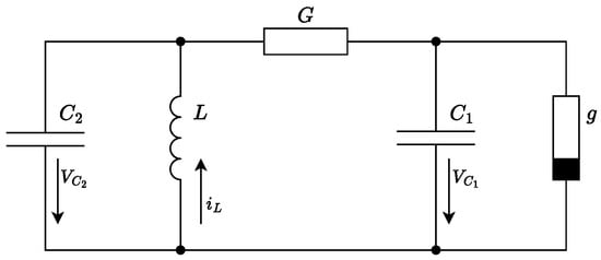
The Chua electric circuit [29] was developed by Leon Chua in the early 1980s to demonstrate chaotic oscillations occurring under certain parameters [32], while a rather similar circuit with a tunnel diode was proposed several years before by Pikovsky and Rabinovich [33]. Nevertheless, Chua’s model quickly gained attention among the scientific community because of its mathematical simplicity and ease of implementation. The canonical Chua circuit design is illustrated in Figure 1.

Figure 1. Schematic diagram of the Chua circuit.

The circuit, depicted in Figure 1, consists of five elements: two capacitors ($C_1$, $C_2$), one inductor (L), a linear resistor (G), and a non-linear negative resistor known as the Chua diode (g). The system of equations used to describe the dynamics of the Chua circuit is as follows:

$$\begin{array}{c}\hfill \left\{\begin{array}{c}{C}_1{\displaystyle \frac{d{V}_{C_1}}{dt}}=(G(V_{C_2}-V_{C_1})-g\left(V_{C_1}\right))\hfill \\ C_2{\displaystyle \frac{d{V}_{C_2}}{dt}}=(G(V_{C_1}-V_{C_2})+i_L)\hfill \\ L{\displaystyle \frac{d{i}_L}{dt}}=-V_{C_2},\hfill \end{array}\right.\end{array}$$

(1)

where $V_{C_1}$ and $V_{C_2}$ represent the voltages across capacitors $C_1$ and $C_2$, respectively, and $i_L$ is the current through the inductor L. The conductance, $G=1/R$, is the reciprocal of the linear resistance R. The term $g\left(V_{C_1}\right)$ is a piecewise-linear function describing the current through the Chua diode as a function of the voltage across it. Its characteristic negative resistance profile is the critical source of the circuit chaotic behavior. This function is typically defined as

$$g\left(V_{C_1}\right)=G_b{V}_{C_1}+{\displaystyle \frac{1}{2}}(G_a-G_b)\left(\right|V_{C_1}+E|-|V_{C_1}-E\left|\right)$$

(2)

where $G_a$ and $G_b$ are the slopes (conductances) of the inner and outer regions of the piecewise-linear curve, respectively, and $\pm E$ are the breakpoints.

2.2. Practical Circuit Design

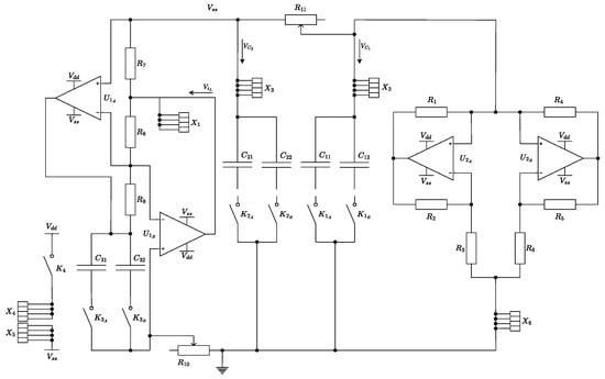
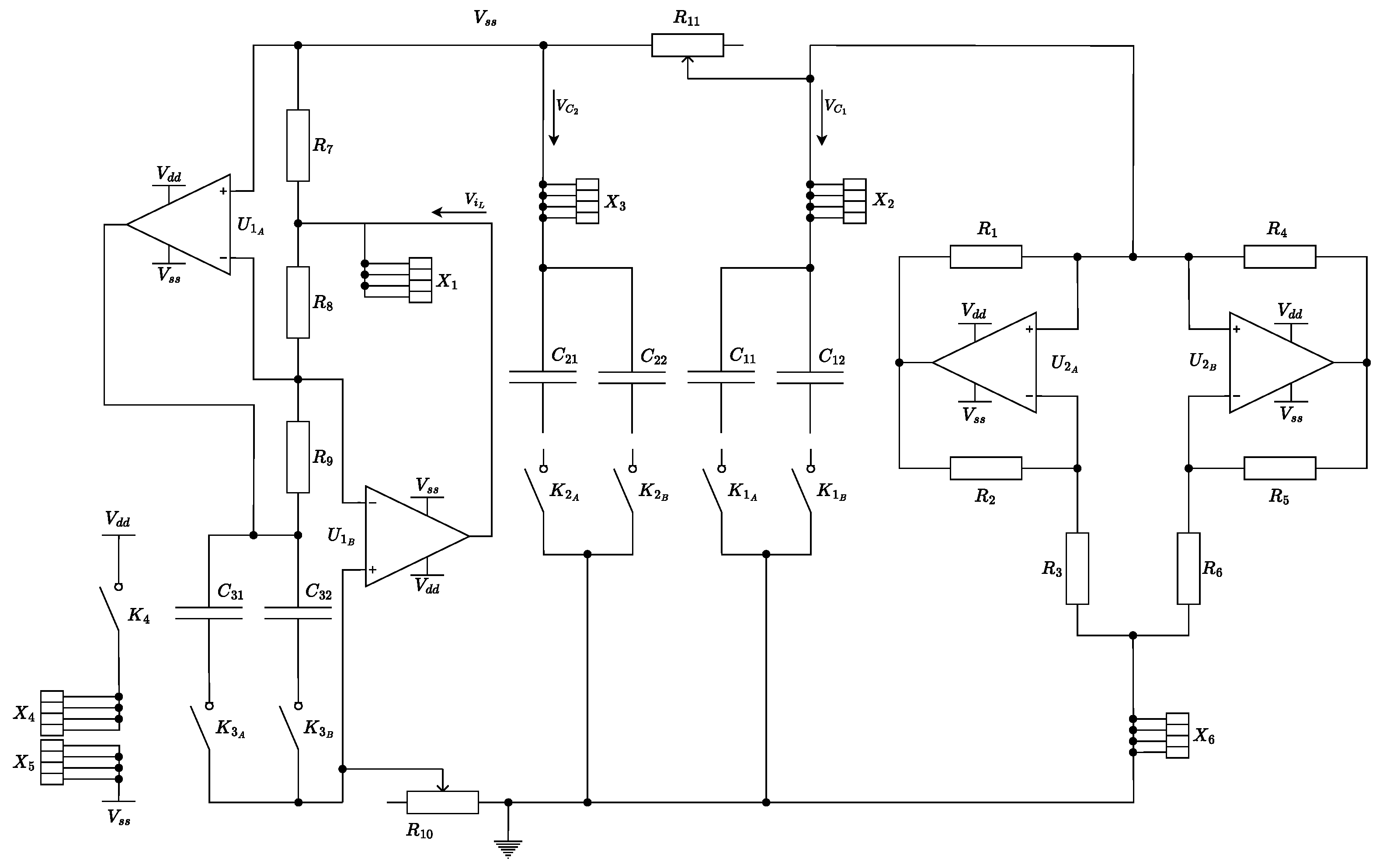
The circuit design proposed in this paper differs from the canonical implementation in several aspects, as one can see from a practically implemented circuit design, given in Figure 2.

Figure 2. Complete schematics of the modified Chua circuit. Switched capacitor banks for $C_1$ and $C_2$ and potentiometers for R and $R_{10}$ allow for external control over the circuit’s dynamics and imitation of input impact as if the circuit is used as a sensor. Terminals $X_1$–$X_6$ provide access to all state variables. Keys $K_{i_A}$ and $K_{i_B}$ ($i\in$ [1…3]) are physically implemented as on-board switches, and also allow for connecting fast electronic keys for imitating the capacitive sensor operation.

First, the Chua diode is implemented using a practical op-amp-based negative impedance converter (NIC) circuit. This active topology reliably synthesizes the required non-linear I-V characteristic using only operational amplifiers and linear resistors. Its special feature is that it can be naturally implemented using one or several memristors [34,35], while the commercially available memristors are still unreliable and expensive. Therefore, we focus on a conventional op-amp implementation, which can be seen on the right side of the circuit, including op-amps $U_{2_A}$ and $U_{2_B}$ in Figure 2.

Second, a significant challenge in implementing robust Chua circuits is the physical inductor. Inductors, especially ones possessing high nominal values required for low-frequency operation, are bulky, prone to electromagnetic interference, and exhibit parasitic series resistance that can damp the chaotic dynamics. To overcome these limitations, the current study employs an active gyrator circuit to emulate the inductive element. A gyrator is an impedance converter that makes a capacitive load appear inductive from the input port. The implemented gyrator-based inductor replacement can be seen on the left side of the circuit, including op-amps $U_{1_A}$ and $U_{1_B}$ in Figure 2.

For this substitution circuit, the equivalent inductance rating is estimated using the following formula:

$$L={\displaystyle \frac{C{R}_7{R}_9{R}_{10}}{R_8}}$$

(3)

In this configuration, C is the physical capacitor in the gyrator circuit, and $R_7$, $R_8$, $R_9$, and $R_{10}$ are resistors that set the gain and impedance scaling. This substitution yields a compact, integrated, and low-interference emulation of an inductive element, whose value can be easily tuned by adjusting, for instance, the potentiometer $R_{10}$.

A primary objective of this experimental setup is to interface the analog chaotic oscillator with a digital system (e.g., an FPGA for neuromorphic processing). To accommodate the sampling rate limitations of typical analog-to-digital converters (ADCs), the circuit was deliberately designed to operate at slower, controllable frequencies. This is achieved by exploiting a key property of the system governing equations. Inspecting Equation (1), it is evident that the rates of change for each state variable are scaled by the factors $1/C_1$, $1/C_2$, and $1/L$, respectively. Consequently, scaling all three reactive components by a common factor n (i.e., $C_1^{\prime }=n{C}_1$, $C_2^{\prime }=n{C}_2$, and $L^{\prime }=nL$) will slow the entire system dynamics by the same factor n, without altering the shape of the chaotic attractor. This principle is applied directly in the modified circuit.

To implement this scaling, capacitors $C_1$ and $C_2$ are realized as parallel banks with DIP switches, allowing their effective capacitance to be changed manually. Furthermore, for maximum experimental flexibility, the critical linear resistor R and the gyrator resistor $R_{10}$ (which controls the emulated inductance L) are implemented as precision potentiometers. All three state variables ($V_{C_1}$, $V_{C_2}$, and $i_L$) are made accessible via dedicated test points for direct observation and data acquisition. The complete list of circuit elements for the modified circuit is provided in Table 1. Note the capacitors in pairs $C_{i1}-C_{i2}$, where $i\in$ [1…3] have identical nominal values but different actually measured values, e.g., $C_{21}=1.00$ uF, $C_{22}=1.03$ uF. This is made for imitating the Chua-circuit based capacitive sensor operation when such subtle changes in capacitance value should be reliably captured.

Table 1. List of circuit components.

Element	Rating	Accuracy	Nominal Value	Units
$R_1$	0.25 W	1%	220	Ohm
$R_2$	0.25 W	1%	220	Ohm
$R_3$	0.25 W	1%	2.2	kOhm
$R_4$	0.25 W	1%	22	kOhm
$R_5$	0.25 W	1%	22	kOhm
$R_6$	0.25 W	1%	3.3	kOhm
$R_7$	0.25 W	1%	100	Ohm
$R_8$	0.25 W	1%	1	kOhm
$R_9$	0.25 W	1%	1	kOhm
$R_{10}$	0.1 W	−	5 (pot.)	kOhm
R	0.1 W	−	5 (pot.)	kOhm
$C_{11}$	100 V	5–10%	0.1	uF
$C_{12}$	100 V	5–10%	0.1	uF
$C_{21}$	100 V	5–10%	1	uF
$C_{22}$	100 V	5–10%	1	uF
$C_{31}$	100 V	5–10%	1	uF
$C_{32}$	100 V	5–10%	1	uF
$U_1$	−	−	TL072CP	−
$U_2$	−	−	TL072CP	−

Initial prototyping of this design was conducted on a National Instruments Elvis III platform (Austin, TX, USA). While the integrated power supplies and data acquisition capabilities of Elvis III were advantageous, the breadboarded version exhibited jitter and unstable dynamics, likely due to parasitic capacitance and poor contact reliability. To ensure signal integrity and reproducibility, a dedicated two-layer printed circuit board (PCB) was designed and fabricated.

2.3. Synchronization Circuit

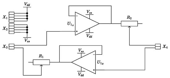
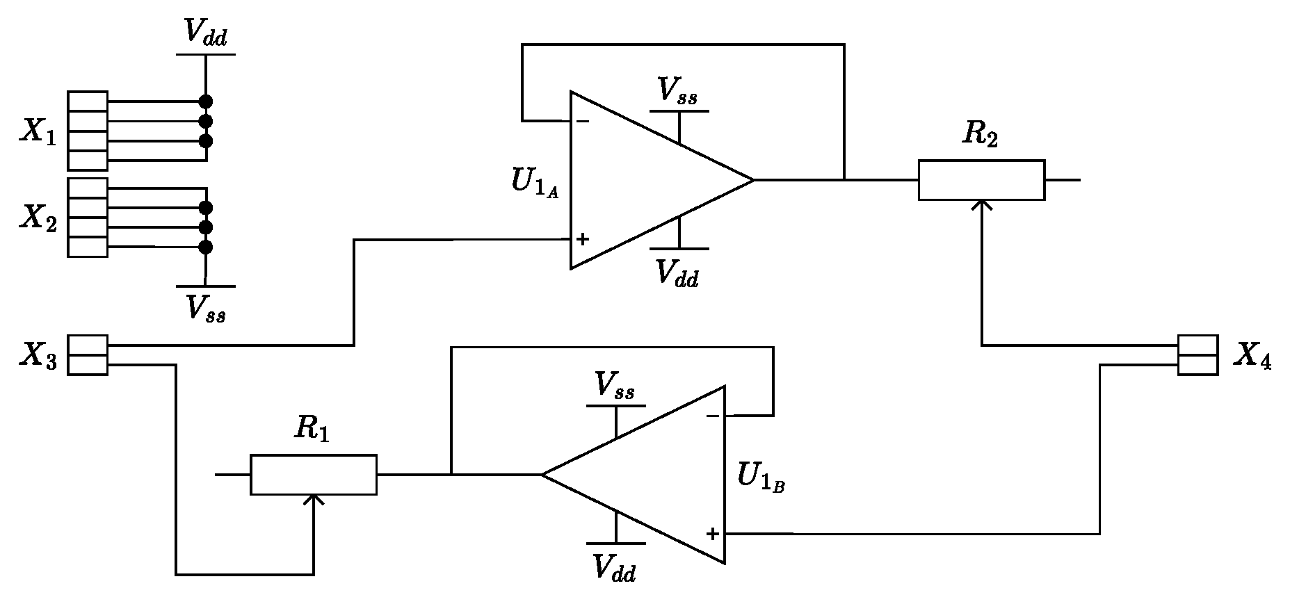
To investigate synchronization phenomena, a simple yet effective unidirectional coupling circuit was designed. This circuit allows the voltage signal from a master oscillator to be injected into a slave oscillator with a controllable coupling strength. As shown in Figure 3, the core of the synchronizing interface is a voltage follower (buffer) built using one-half of a TL072CP operational amplifier. This buffer ensures that the coupling circuit presents a high input impedance to the master oscillator, preventing loading effects. The buffered signal is then passed through a potentiometer ($R_1$ or $R_2$), which acts as a voltage divider to precisely control the coupling coefficient. The output of the potentiometer is then connected directly to the corresponding node (e.g., $V_{C_1}$) of the slave circuit. A second, identical circuit is included on the same board using the second op-amp in the DIP-8 package, allowing for independent coupling of multiple state variables. The list of circuit elements for this interface is minimal, as listed in Table 2.

Figure 3. Schematic of the coupling circuit used for synchronization experiments. Potentiometers $R_1$ and $R_2$ provide independent control over the coupling strength for two separate channels (in further experiments, only one channel is used).

Table 2. Component list for the synchronization interface circuit.

Element	Rating	Accuracy	Value	Units
$R_{10}$	0.1 W	−	5 (pot.)	kOhm
R	0.1 W	−	5 (pot.)	kOhm
$U_1$	−	−	TL072CP	−

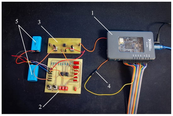
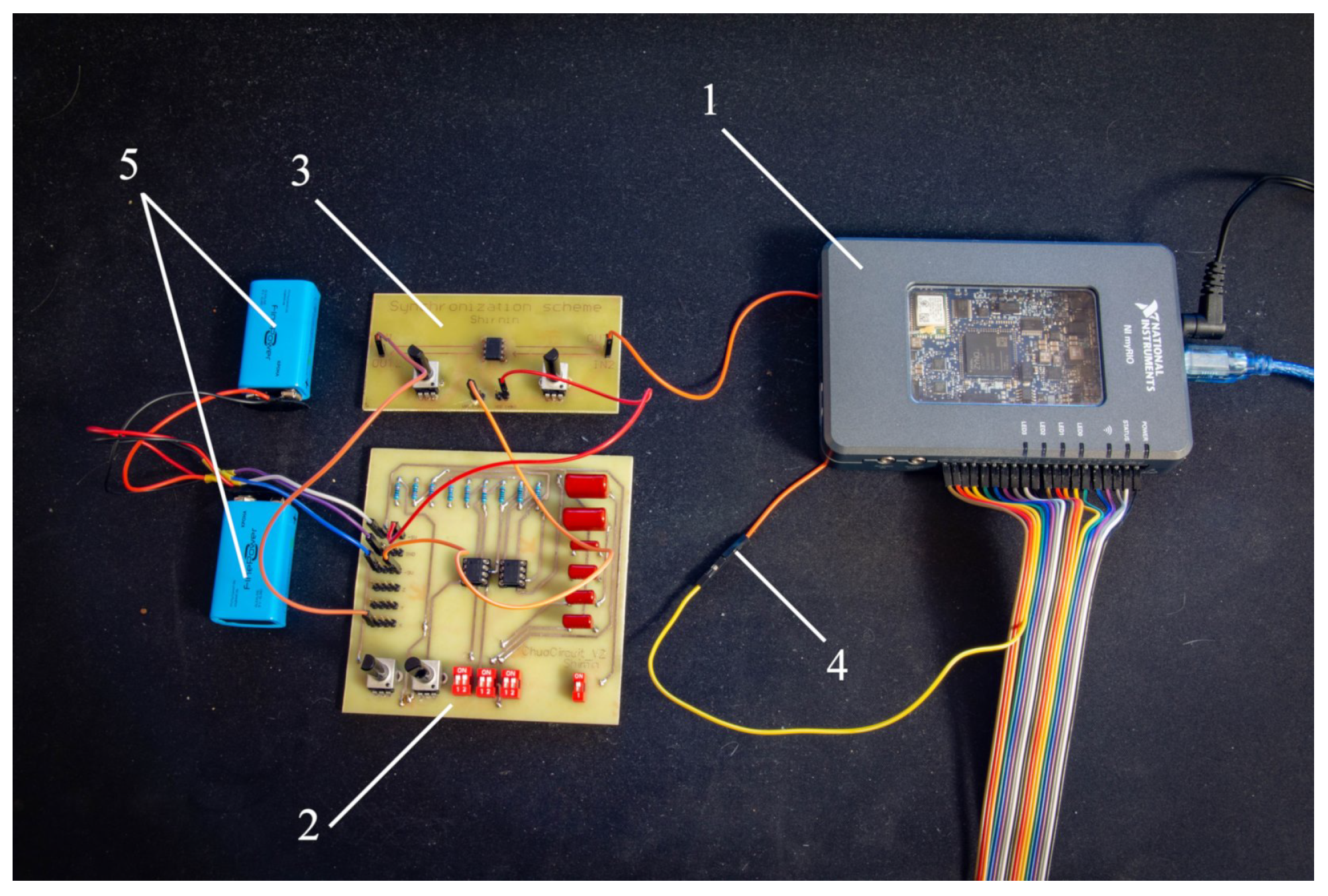
This synchronization circuit was also implemented on a compact PCB, designed for direct integration with the main Chua circuit board. The final test bench including the Chua circuit, the coupling circuit, the power supply, and the digital controller NI MyRIO-1900 with an on-board FPGA is given in Figure 4.

Figure 4. The developed test bench for chaotic synchronization. The numbers denote (1) NI myRIO-1900, (2) the modified Chua circuit, (3) the synchronization board, (4) the datastream wire in configuration when MyRIO is master and the analog board is slave, and (5) batteries providing stable $V_{dd}$, $V_{ss}$ and zero voltages.

2.4. Chua Circuit Identification and Model Analysis

To obtain an accurate mathematical model of the physical Chua circuit described in Section 2.1, a system identification procedure was performed. Time-series data of the three state variables $V_{C_1}$, $V_{C_2}$, and $V_{i_L}$ were acquired from the fabricated PCB via a data acquisition system employing the NI myRIO-1900 controller. These data were subsequently processed using the ODERECON software package for MATLAB 2021b (https://github.com/aikarimov/ODERECON accessed on 15 April 2026), a specialized tool designed for the reconstruction of ordinary differential equations (ODEs) from empirical time-series measurements.

The sampling frequency was set to f = 100,251 samples/sec, which provides a reasonable tradeoff between the time resolution and the length of the record, limited by 10,000 samples. With the specified sampling frequency, the length of the data series was $0.0997$ s.

The software package ODERECON employs a least squares approach with an adaptive thresholding algorithm [36,37,38] to estimate the sparse dynamical models, finding coefficients that best describe the observed dynamics in terms of polynomial dynamical systems. To work with the piecewise-linear system, this software was appropriately modified, and the identification process became two-stage in a manner close to a pipeline proposed in [39]. At the first stage, the breakpoints $E_n$ (negative) and $E_p$ (positive) associated with the nonlinear function $g\left(V_{C_1}\right)$ are estimated via iteratively reweighted least squares. At the second stage, the software identifies the underlying dynamics of each section, assuming it may contain additional polynomial nonlinearities. From previous works, it is known that the real dynamics of circuits are much more complicated than the original equations in terms of polynomial functions [28,31]. Interesting to note, in the case of the identified Chua circuit, the proper setting of the thresholding parameter $\eta =1.0$ resulted in no additional nonlinear terms in the model.

To maintain consistency with the conventional notation, we hereafter denote the state variables as x, y and z. As usual, we take $x=V_{C_1}$, and $y=V_{C_2}$. The third variable is originally associated with current $z=i_L$, but in our study, z was collected as $U_{1_B}=V_{i_L}$ measured at terminal $X_1$, see Figure 2, and therefore represents a linear transformation of $i_L$.

A key characteristic of the Chua circuit is that the nonlinearity is confined to the first equation, which reads differently for different regions in the nonlinear function domain. The breakpoints delimiting the regions were identified as $E_n=-0.9$ and $E_p=1.0$.

For the outer left region ($x<E_n$), the equations read

$$\begin{array}{cc}\hfill \dot{x}& =a_n+b_{n}x+c_{n}y.\hfill \end{array}$$

(4)

For the outer right region ($x>E_p$),

$$\begin{array}{cc}\hfill \dot{x}& =a_p+b_{p}x+c_{p}y.\hfill \end{array}$$

For the inner region ($E_n\le x\le E_p$),

$$\begin{array}{cc}\hfill \dot{x}& =a_c+b_{c}x+c_{c}y+d_{c}z.\hfill \end{array}$$

The equations for $\dot{y}$ and $\dot{z}$

$$\begin{array}{cc}\hfill \dot{y}& =p_{y}x+q_{y}y+r_{y}z\hfill \end{array}$$

(5)

$$\begin{array}{cc}\hfill \dot{z}& =p_{z}x+q_{z}y+r_{z}z\hfill \end{array}$$

(6)

remain invariant across all three regions.

The identified numerical values of the parameters are as follows. The parameters for the outer left region ($x<E_n$) are

$$\begin{array}{cc}\hfill a_n& =-2956.4381,b_n=-1133.7795,c_n=4892.6766.\hfill \end{array}$$

For the outer right region ($x>E_p$),

$$\begin{array}{cc}\hfill a_p& =3140.4641,b_p=-1149.9195,c_p=4894.9515.\hfill \end{array}$$

For the inner region ($E_n\le x\le E_p$),

$$\begin{array}{cc}\hfill a_c& =-38.7605,b_c=2065.6838,c_c=5031.1177,d_c=-122.2301.\hfill \end{array}$$

The parameters governing the dynamics of the y and z variables are consistent across all regions:

$$\begin{array}{cc}\hfill p_y& =452.7923,q_y=-8916.0849,r_y=8480.8662,\hfill \\ \hfill p_z& =452.0403,q_z=-9447.7078,r_z=8465.1742.\hfill \end{array}$$

The major difference between the obtained model and the canonical Chua circuit (1) is the form of equation for $\dot{z}$, defined by (6) in our model. Nevertheless, the piecewise-linear form of the model allows for its detailed analysis similar to the original Chua circuit.

2.5. Synchronizability Analysis

To study the synchronization of two identical Chua circuits, we consider a master–slave configuration. Let the master system be denoted by the state vector ${\mathbf{x}}_m={(x_m,y_m,z_m)}^T$ and the slave system by ${\mathbf{x}}_s={(x_s,y_s,z_s)}^T$, both governed by the identified dynamics. The coupling is introduced unidirectionally from the master to the slave. We investigate three distinct coupling schemes through state variables: coupling through the x, y, and z variables.

First, we define the error vector $\mathbf{e}={\mathbf{x}}_m-{\mathbf{x}}_s={(e_x,e_y,e_z)}^T$. The goal of synchronization is to achieve $\mathbf{e}\to 0$ as $t\to \infty$.

2.5.1. Coupling via the x Variable

In this scheme, the coupling signal is proportional to the difference in the x variables. The slave system is modified by the injection of the term $k_x(x_m-x_s)$ into its ${\dot{x}}_s$ equation. The equations for the slave system become

$$\begin{array}{cc}\hfill {\dot{x}}_s& =f_x\left({\mathbf{x}}_s\right)+k_x(x_m-x_s)\hfill \\ \hfill {\dot{y}}_s& =f_y\left({\mathbf{x}}_s\right)\hfill \\ \hfill {\dot{z}}_s& =f_z\left({\mathbf{x}}_s\right)\hfill \end{array}$$

(7)

where $f_x$, $f_y$, and $f_z$ represent the right-hand sides of the identified model for the respective state variables. The coupling strength is denoted by $k_x\ge 0$. The corresponding error dynamics are derived by subtracting the master equations from the slave equations. Assuming both systems operate in the same linear region (a valid assumption for the stability analysis near the synchronization manifold), the error dynamics can be linearized to $\dot{\mathbf{e}}=\mathbf{J}\mathbf{e}$, where $\mathbf{J}$ is the Jacobian matrix of the slave system evaluated on the synchronization manifold, modified by the coupling. For x-coupling in forward-time direction, this matrix is

$${\mathbf{J}}_x^F=\left(\begin{array}{ccc}{\displaystyle \frac{\partial f_x}{\partial x}}-k_x^F& {\displaystyle \frac{\partial f_x}{\partial y}}& {\displaystyle \frac{\partial f_x}{\partial z}}\\ {\displaystyle \frac{\partial f_y}{\partial x}}& {\displaystyle \frac{\partial f_y}{\partial y}}& {\displaystyle \frac{\partial f_y}{\partial z}}\\ {\displaystyle \frac{\partial f_z}{\partial x}}& {\displaystyle \frac{\partial f_z}{\partial y}}& {\displaystyle \frac{\partial f_z}{\partial z}}\end{array}\right).$$

(8)

It is different for different regions of the nonlinear function. For example, for the outer left region $x<E_n$, from (4)–(6), we have

$${\mathbf{J}}_x^F{|}_{x<E_n}=\left(\begin{array}{ccc}{b}_n-k_x^F& c_n& 0\\ p_y& q_y& r_y\\ p_z& q_z& r_z\end{array}\right).$$

(9)

Synchronization stability requires that all eigenvalues of ${\mathbf{J}}_x^F$ have negative real parts. The characteristic polynomial of this $3\times 3$ matrix is of the form

$$P_x^F\left(\lambda \right)={\lambda }^3+{\alpha }_1\left(k_x\right){\lambda }^2+{\alpha }_2\left(k_x\right)\lambda +{\alpha }_3\left(k_x\right)$$

(10)

where the coefficients ${\alpha }_i$ are functions of the system parameters and the coupling strength $k_x^F$. According to the Routh–Hurwitz criterion, the necessary and sufficient condition for all roots to have negative real parts is that all principal minors of the Hurwitz matrix are positive. This yields the following conditions for a given set of identified parameters:

$$\left\{\begin{array}{c}{\alpha }_1\left(k_x\right)>0\hfill \\ {\alpha }_3\left(k_x\right)>0\hfill \\ {\alpha }_1\left(k_x\right){\alpha }_2\left(k_x\right)-{\alpha }_3\left(k_x\right)>0\hfill \end{array}\right.$$

(11)

By substituting the identified numerical parameters from Section 3.1 into these inequalities, a critical coupling strength $k_x^{Fcrit}$ can be determined, above which the synchronized state becomes stable. Analysis of the identified model predicts a threshold for x-coupled synchronization.

Numerical results for positive $k_x^F$ are

$$k_x^{Fcrit}\approx \left\{\begin{array}{c}2697,x<E_n\hfill \\ 5898,E_n\le x\le E_p\hfill \\ 2683,x>E_p\hfill \end{array}\right.,$$

which implies the forward-time synchronization would occur for $k_x^F>5898$.

Extending the analysis to backward-time synchronization, we investigate the theoretical possibility of synchronization with negative coupling coefficient ($k_x<0$) and in reverse time ($t\to -\infty$). If the forward-time error dynamics are governed by $\dot{\mathbf{e}}=\mathbf{J}\left(k\right)\mathbf{e}$, this is equivalent to analyzing the forward-time stability of the system $\dot{\mathbf{e}}=-\mathbf{J}(-k)\mathbf{e}$. In our particular case, we have

$${\mathbf{J}}_x^B=-\left(\begin{array}{ccc}{\displaystyle \frac{\partial f_x}{\partial x}}+k_x^B& {\displaystyle \frac{\partial f_x}{\partial y}}& {\displaystyle \frac{\partial f_x}{\partial z}}\\ {\displaystyle \frac{\partial f_y}{\partial x}}& {\displaystyle \frac{\partial f_y}{\partial y}}& {\displaystyle \frac{\partial f_y}{\partial z}}\\ {\displaystyle \frac{\partial f_z}{\partial x}}& {\displaystyle \frac{\partial f_z}{\partial y}}& {\displaystyle \frac{\partial f_z}{\partial z}}\end{array}\right)$$

(12)

Substituting the numerical parameters from Section 3.1, we find no solution for (11) for the characteristic polynomial of (12). While this does not strictly indicate that synchronization would not occur, it means that it is unlikely.

2.5.2. Coupling via the y Variable

Similarly, for coupling solely through the y variable with strength $k_y\ge 0$, the slave system is defined as

$$\begin{array}{cc}\hfill {\dot{x}}_s& =f_x\left({\mathbf{x}}_s\right)\hfill \\ \hfill {\dot{y}}_s& =f_y\left({\mathbf{x}}_s\right)+k_y(y_m-y_s)\hfill \\ \hfill {\dot{z}}_s& =f_z\left({\mathbf{x}}_s\right)\hfill \end{array}$$

The corresponding Jacobian matrix for the error dynamics on the synchronization manifold is

$${\mathbf{J}}_y^F=\left(\begin{array}{ccc}{\displaystyle \frac{\partial f_x}{\partial x}}& {\displaystyle \frac{\partial f_x}{\partial y}}& {\displaystyle \frac{\partial f_x}{\partial z}}\\ {\displaystyle \frac{\partial f_y}{\partial x}}& {\displaystyle \frac{\partial f_y}{\partial y}}-k_y^F& {\displaystyle \frac{\partial f_y}{\partial z}}\\ {\displaystyle \frac{\partial f_z}{\partial x}}& {\displaystyle \frac{\partial f_z}{\partial y}}& {\displaystyle \frac{\partial f_z}{\partial z}}\end{array}\right)$$

(13)

Applying the Routh–Hurwitz stability criteria to the characteristic polynomial of ${\mathbf{J}}_y^F$ allows for the determination of a critical coupling strength $k_y^{Fcrit}$ for y-coupled synchronization. Nevertheless, in forward direction, there are no solutions to (11) for the characteristic polynomial of (13). This was described by L. Chua et al. in their 1993 work on synchronization in the Chua system [29]. Nevertheless, numerical and physical experiments revealed that the original Chua system can synchronize by y variable [29].

The backward-time Jacobian matrix for the error dynamics on the synchronization manifold is

$${\mathbf{J}}_y^B=-\left(\begin{array}{ccc}{\displaystyle \frac{\partial f_x}{\partial x}}& {\displaystyle \frac{\partial f_x}{\partial y}}& {\displaystyle \frac{\partial f_x}{\partial z}}\\ {\displaystyle \frac{\partial f_y}{\partial x}}& {\displaystyle \frac{\partial f_y}{\partial y}}+k_y^B& {\displaystyle \frac{\partial f_y}{\partial z}}\\ {\displaystyle \frac{\partial f_z}{\partial x}}& {\displaystyle \frac{\partial f_z}{\partial y}}& {\displaystyle \frac{\partial f_z}{\partial z}}\end{array}\right)$$

(14)

The solution can be found only for the central fragment $E_n\le x\le E_p$, with numerical value as $k_y^{Bcrit}\approx 784$. This interesting result provides the theoretical substantiation of the synchronization possibility in time-reversible framework by y variable.

2.5.3. Coupling via the z Variable

When coupled through the z variable with strength $k_z\ge 0$, the slave system reads as

$$\begin{array}{cc}\hfill {\dot{x}}_s& =f_x\left({\mathbf{x}}_s\right)\hfill \\ \hfill {\dot{y}}_s& =f_y\left({\mathbf{x}}_s\right)\hfill \\ \hfill {\dot{z}}_s& =f_z\left({\mathbf{x}}_s\right)+k_z(z_m-z_s)\hfill \end{array}$$

Similar analysis applied to the coupling via z variable reveals that forward-time direction allows synchronization in left and right regions with the coupling strengths

$$k_z^{Fcrit}\approx \left\{\begin{array}{c}52.9,x<E_n\hfill \\ 54.1,x>E_p\hfill \end{array}\right.,$$

and yields no solutions for backward-time direction.

It is important to emphasize that the Routh–Hurwitz stability analysis presented above provides a local criterion valid only in the vicinity of the synchronization manifold and under the assumption that both systems remain within the same piecewise-linear region. The theoretical thresholds derived here guarantee local error decay but do not characterize the global domain of attraction. The experimental convergence maps presented in Section 3 therefore reflect empirical, global behavior, which is inherently influenced by the bidirectional nature of TRS, chaotic trajectory mixing, and finite-window effects. This distinction is critical for interpreting the practical robustness of the proposed synchronization schemes.

2.6. Time-Reversible Synchronization

Time-reversible synchronization (TRS) is a recently proposed technique that exploits the inherent time-reversibility of dynamical systems and symmetric numerical integrators to achieve super-exponential convergence of synchronized trajectories [26]. Unlike conventional methods operating only in forward time direction $t\to +\infty$, TRS alternates between forward and backward phases within a finite time window.

The core idea involves iteratively propagating the slave system ${\mathbf{x}}_s$ forward and backward in time using a time-reversible numerical method, such as the semi-implicit composition diagonal (CD) method [28]. During the forward phase, the slave is driven by the recorded master signal ${\mathbf{X}}_m={({\mathbf{x}}_m\left[j\right],{\mathbf{x}}_m[j+1],\dots ,{\mathbf{x}}_m[j+n-1])}^T$ consisting of n samples starting from j with a positive definite coupling matrix ${\mathbf{K}}^f$. In the backward phase, the master signal is reversed in time, and a negative definite coupling matrix ${\mathbf{K}}^b$ is applied. Under appropriate conditions, this bidirectional process ensures that the synchronization error decreases in both time directions. The pseudocode for the standard time-reversible synchronization algorithm is presented in Algorithm 1.

Algorithm 1: Time-Reversible Synchronization (TRS) [26]

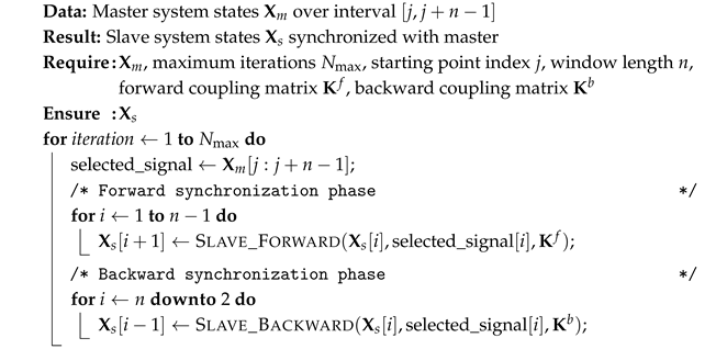The procedures Slave_Forward and Slave_Backward implement one-step numerical integration using a time-symmetric method. For a general chaotic system described by $\dot{\mathbf{x}}=\mathbf{f}\left(\mathbf{x}\right)$, the forward synchronized dynamics are governed by

$${\dot{\mathbf{x}}}_s=\mathbf{f}\left({\mathbf{x}}_s\right)+{\mathbf{K}}^f({\mathbf{x}}_m-{\mathbf{x}}_s),$$

(15)

while the backward synchronized dynamics are given by

$${\dot{\mathbf{x}}}_s=-\mathbf{f}\left({\mathbf{x}}_s\right)-{\mathbf{K}}^b({\mathbf{x}}_m-{\mathbf{x}}_s).$$

(16)

The coupling matrices ${\mathbf{K}}^f$ and ${\mathbf{K}}^b$ are typically diagonal, with nonzero elements corresponding to the specific state variable used for synchronization. In the case of a single synchronization variable, they become scalars.

Despite its theoretical advantages, the standard TRS algorithm possesses a critical limitation: synchronization is not achievable from all regions of the attractor. As found in the previous studies [26,28], certain initial conditions lead to divergence during either the forward or backward phase, making the method impractical for almost any real applications where the starting point cannot be arbitrarily chosen.

To address this limitation, a practically feasible heuristic algorithm for time-reversible synchronization (PFHa-TRS) was proposed in [28]. This algorithm merges the super-exponential convergence of TRS with the robust stability of the conventional Pecora–Carroll (P-C) synchronization, providing an adaptive intervention mechanism. The algorithm tries to achieve low synchronization error from the current point using the TRS method, but if after a predefined number of iterations the synchronization error exceeds a predefined threshold, the algorithm temporarily switches to P-C synchronization, makes one step forward, and resumes the TRS process. This hybrid approach ensures convergence from any initial condition while maintaining the rapid synchronization rate characteristics. The pseudocode for the PFHa-TRS algorithm is provided in Algorithm 2.

Algorithm 2: Practically Feasible Heuristic Algorithm for Time-Reversible Synchronization (PFHa-TRS) [28]

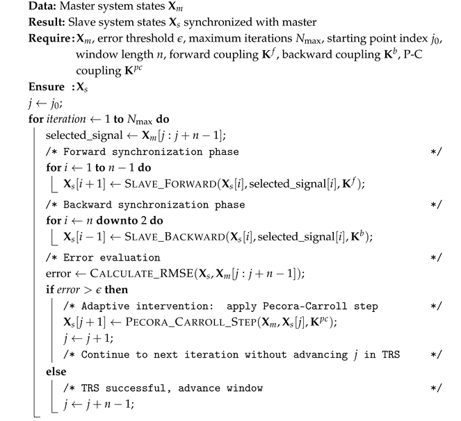In Algorithm 2, the Calculate_RMSE function computes the root mean square error between the slave trajectory and the corresponding master segment. The Pecora_Carroll_Step function implements a single forward step of conventional dissipative synchronization:

$${\dot{\mathbf{x}}}_s=\mathbf{f}\left({\mathbf{x}}_s\right)+{\mathbf{K}}^{pc}({\mathbf{x}}_m-{\mathbf{x}}_s),$$

(17)

typically with a large coupling gain to ensure rapid error reduction. The adaptive switching mechanism guarantees that even if the TRS process begins to diverge (indicated by error exceeding $ϵ$), the algorithm can recover stability through the P-C intervention. This heuristic approach effectively eliminates the need for proper initial conditions while preserving the super-exponential convergence rate of pure TRS in regions where it performs well.

3. Results

This section presents the experimental results, both in fundamental properties of time-reversible synchronization and in a practical sensing application.

3.1. Synchronization in Case of Different Couplings

The performance of both conventional dissipative coupling (Pecora–Carroll) and time-reversible synchronization (TRS) was evaluated for the identified model of the modified Chua circuit described in Section 2. Experiments were conducted for three distinct coupling schemes, utilizing each of the state variables (x, y, and z) as the single synchronization channel.

For hardware implementation and real-time validation, the identified model was deployed on a National Instruments MyRIO-1900 platform, which integrates a dual-core ARM Cortex-A9 processor with an FPGA Xilinx Zynq-7010. The FPGA was programmed to implement the CD2 time-symmetric numerical integration method [28], so that the digital platform could play the role of both master or slave systems. Due to the fixed-point arithmetic constraints of the FPGA and the need for efficient resource utilization, all identified model parameters from Section 2 were rounded to the nearest integer values. This rounding operation, while potentially introducing minor discrepancies, remained within acceptable bounds for maintaining chaotic dynamics and synchronization performance, as we will see further.

The FPGA implementation was synthesized using Xilinx Vivado 2022.1 targeting the Zynq-7010 SoC on the NI MyRIO-1900 platform. Table 3 summarizes the hardware resource utilization and timing performance of the CD integrator combined with the PFHa-TRS control logic. The design operates at a system clock of 100 MHz, comfortably meeting the 100.251 kSamples/s data acquisition requirement while leaving sufficient headroom for future extensions.

Table 3. Utilization of FPGA Xilinx Zynq-7010 resources.

Device Utilization	Used	Total	Percent
Total Slices	3790	4400	86.1
Slice Registers	11,635	35,200	33.1
Slice LUTs	12,022	17,600	68.3
DSP48s	32	80	40.0
Block RAMs	5	60	8.3

3.1.1. Synchronization via x Variable Coupling

The first coupling configuration employed dissipative coupling through the x variable only. For the identified Chua circuit model, forward synchronization via x was found to be highly effective. A coupling gain of $k_x=5\times {10}^4$ ensured rapid convergence of the slave system state to the master trajectory, with synchronization errors decaying approximately to the noise level after a $0.03$ s transient.

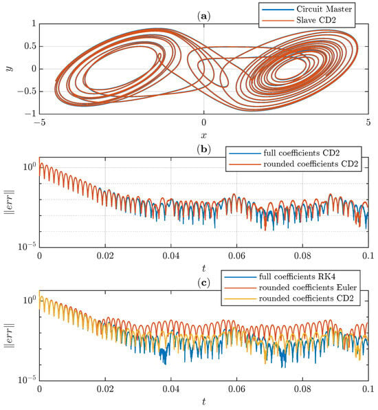
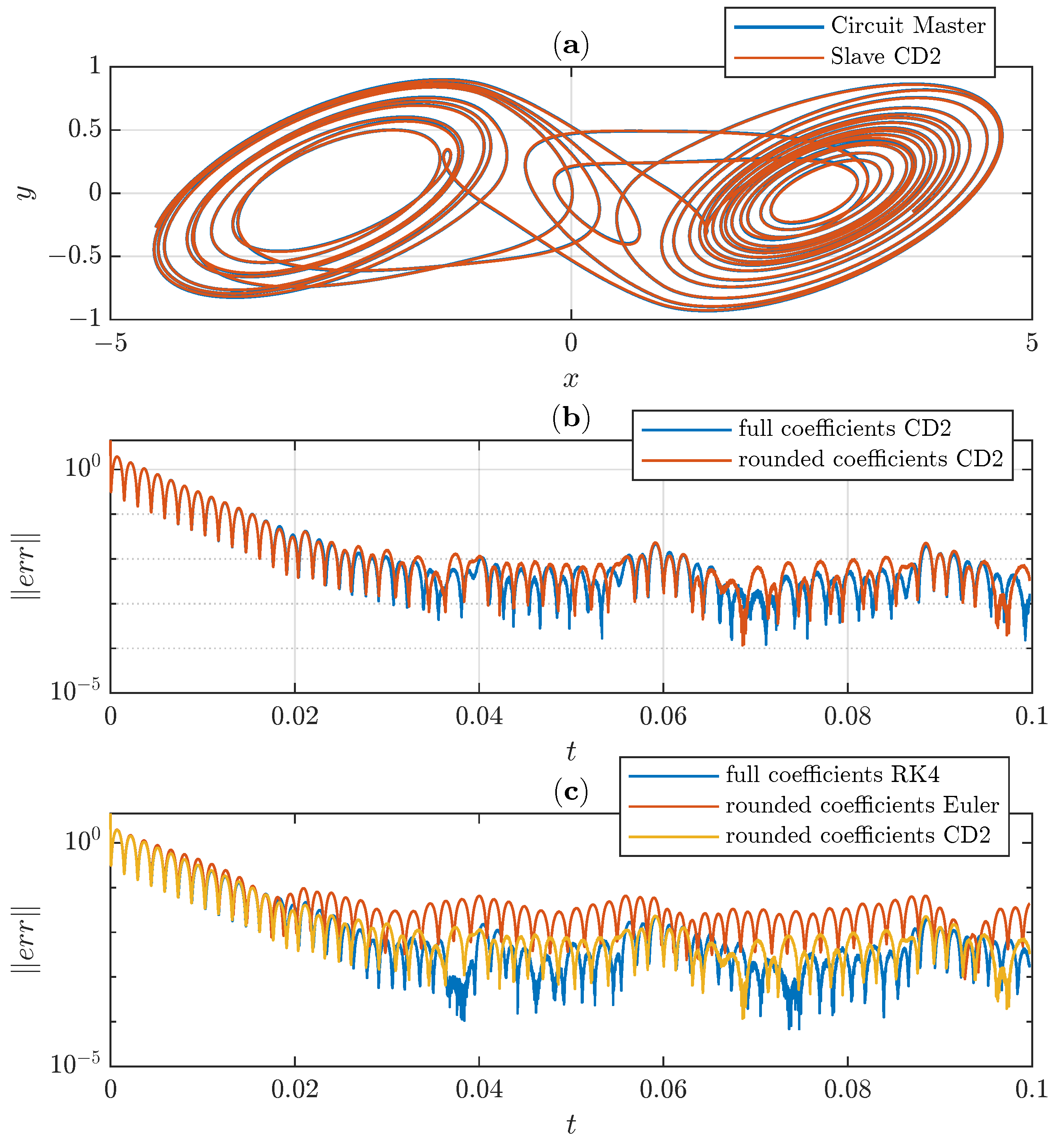
To make a ubiquitous comparison of different synchronization conditions, we took three numerical methods and used full coefficients and rounded integer coefficients suitable for uploading to the limited-resource FPGA. The results are given in Figure 5, explicitly demonstrating that the second-order CD2 method is enough for the proposed embedded application, while the first-order Euler method lacks accuracy. The fourth-order RK4 method implemented in a manner proposed in [31] turns out to be too complicated and yields no additional accuracy.

Figure 5. Analog-to-digital synchronization via x variable. Panel (a) illustrates the $x-y$ phase space; Panel (b) compares two implementations of the slave system with the CD2 method, with full and rounded coefficients; and Panel (c) compares the Euler, CD2, and RK4 methods. One clearly sees no explicit difference between RK4 and CD2 methods.

We also tested the RK2 (explicit midpoint) method, which gave the results similar to the results of CD2.

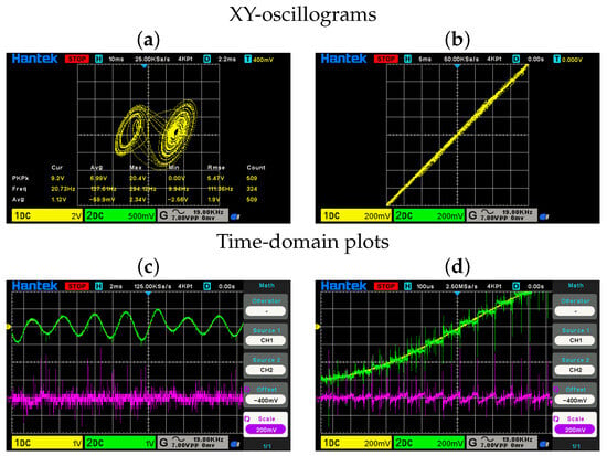
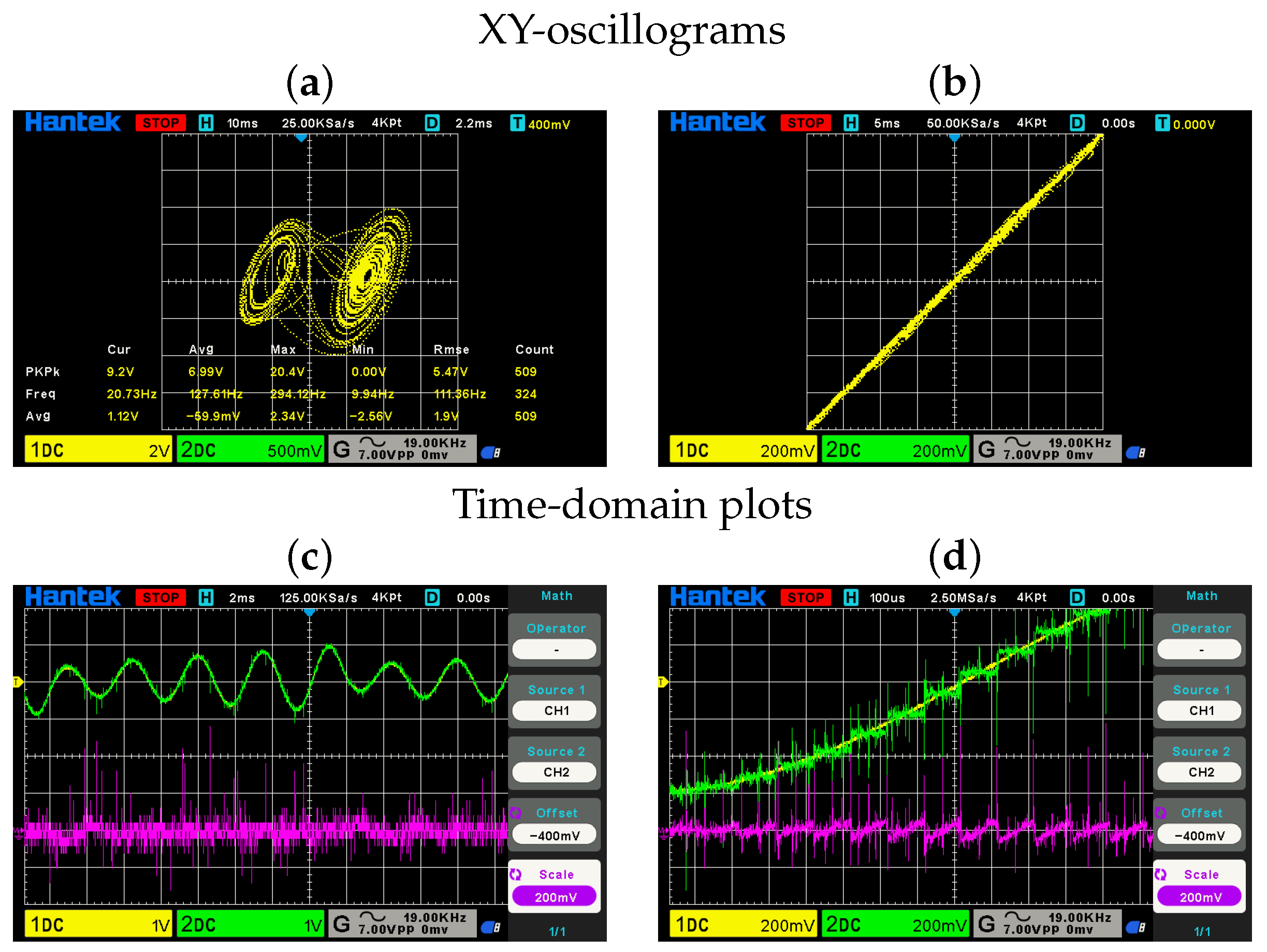
Figure 6 illustrates the synchronization performance in a digital-to-analog (master: digital model, slave: physical circuit) configuration. The time-reversible CD2 integration method proved stable for the bidirectional synchronization. The MyRIO-1900 platform successfully executed the real-time synchronization at a sampling rate of $100.251$ kSamples/s, demonstrating the practical feasibility of the approach for embedded applications.

Figure 6. Dissipative digital-to-analog synchronization between the digital model implemented in MyRIO-1900 and the analog circuit. Panel (a) gives the experimental snapshot of the analog attractor in variables x and y captured with Hantek DSO2D15 oscilloscope. Panel (b) illustrates the synchronized state in y variables of slave (horizontal) and master (vertical) axes, when the systems are x-coupled. Panel (c) illustrates time evolution of y variables (yellow for the slave, green for the master, magenta for error), and panel (d) gives zoom-in of the plot in panel (c). Discrete levels of the digital system are clearly visible; nevertheless, the discontinuous behavior of the master signal has no affect in y variable of the slave system.

However, when applying the standard time-reversible synchronization algorithm to the x-coupled configuration, time-reversible synchronization failed to converge for any settings. Analysis revealed that the failure occurred due to instability in the backward phase, where the time-reversed dynamics of the x-coupled system were unstable by the Routh–Hurwitz criterion, as described in Section 2. This observation outlines once again the critical dependence of the TRS on the specific system dynamics and prevents the use of the PFHa-TRS algorithm in the case of x-coupling.

3.1.2. Synchronization via y Variable Coupling

Conventional dissipative coupling through the y variable alone proved the absence of synchronization for the identified Chua circuit model with any positive coupling gain $K_y>0$, unlike the situation with the original Chua system [29]. This behavior is consistent with the theoretical analysis presented in Section 2.

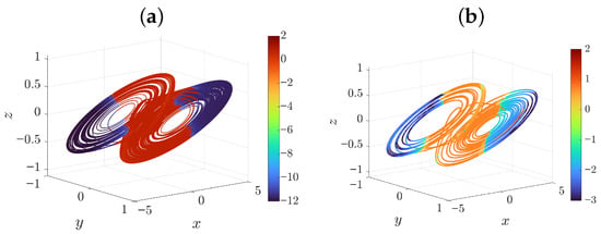
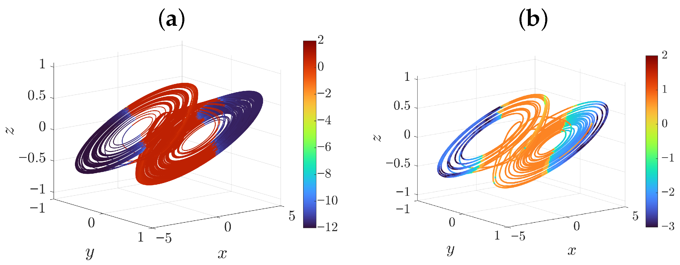
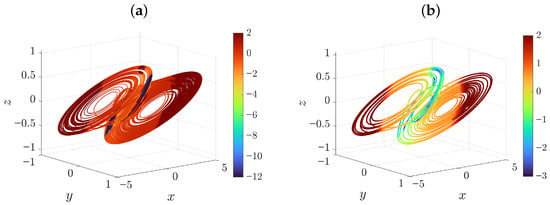
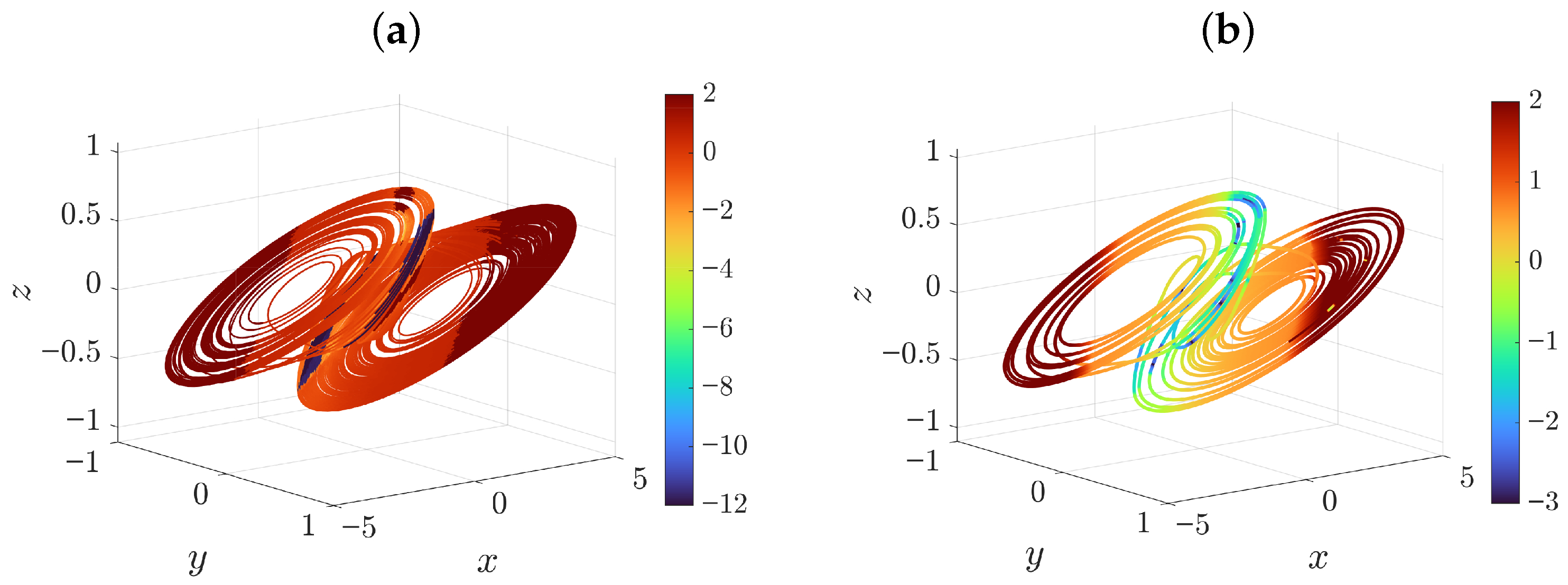
In contrast to conventional coupling, time-reversible synchronization demonstrated remarkable efficiency for y-variable coupling. Figure 7 displays the synchronization regions in the attractor for TRS with y-coupling. The color mapping indicates the achieved ${log}_{10}$ error norm from each initial condition, with blue representing complete synchronization and red representing the absence of convergence, both after 2000 iterations. Notably, substantial portions of the attractor exhibit successful TRS convergence, despite the complete failure of conventional dissipative y-coupling. This finding highlights the unique advantage of time-reversible methods: by operating in both time directions, TRS can stabilize synchronization channels that are inherently unstable in forward time alone.

Figure 7. Panel (a) illustrates synchronization via y variable between two digital models. Color indicates ${log}_{10}$ error norm from each points after 2000 iterations. Panel (b) illustrates synchronization via y variable coupling with analog circuit as the master and the digital model as the slave. Synchronization coefficients are $K_y^f=K_y^b=200$.

3.1.3. Synchronization via z Variable Coupling

The third coupling configuration utilized dissipative coupling through the z variable. For the identified model, forward synchronization via z with conventional coupling proved to be not entirely effective. A moderate gain of $K_z=2500$ allowed for achieving complete synchronization in left and right regions of nonlinear function $g\left(x\right)$, corresponding to the attractor scrolls, but the slave system was losing synchronization in the transition phase between scrolls, which fully coincides with theoretical results in Section 2. The convergence rate was similar to x-coupling.

Time-reversible synchronization was also successful for z-variable coupling, though with more restricted convergence regions compared to the y-coupled case. Figure 8 maps the synchronization performance of TRS with z-only coupling across the attractor. The regions of successful convergence (colored blue) are much smaller than those observed for y-coupling, with mostly red regions indicating initial conditions from which TRS diverges. This behavior can be attributed to the structure of the error dynamics for z-coupling, where the backward synchronization phase requires relatively high coupling gains to ensure stability.

Figure 8. Synchronization via z variable coupling: regions of convergence for time-reversible synchronization. Colored regions indicate successful synchronization, with blue representing fastest convergence and red representing the absence of convergence. The convergence regions are much smaller than for y-coupling. Panel (a) illustrates synchronization between two digital models. Color indicates ${log}_{10}$ error norm from each point after 2000 iterations. Panel (b) illustrates synchronization via z variable with analog circuit as the master and the digital model as the slave. Synchronization coefficients are $K_z^f=K_z^b=200$.

Table 4 summarizes the synchronization performance for the three coupling schemes, comparing conventional dissipative coupling with time-reversible synchronization. The results demonstrate that while conventional coupling is effective for x and z variables, it fails completely for y-variable coupling. Time-reversible synchronization, by contrast, succeeds for all three variables, though with varying convergence regions. The PFHa-TRS algorithm described in Section 2.5 effectively combines the advantages of both approaches, ensuring convergence from any initial condition while maintaining the rapid synchronization rates of TRS in favorable regions.

Table 4. Summary of qualitative synchronization performance for different coupling variables.

Coupling	P-C	TRS	P-C Conv.	TRS Conv.
Variable	Synchronization	Synchronization	Regions	Regions
x	Successful	Fails	All attractor	None
y	Fails	Successful	None	Large
z	Successful	Successful	Fragmented	Fragmented

The experimental validation on the NI MyRIO-1900 platform confirmed that the integer-rounded parameters and CD2 integration method preserve the essential synchronization properties identified in simulation. The FPGA implementation achieved real-time performance with negligible latency, demonstrating the suitability of the proposed approaches for embedded neuromorphic sensor applications where rapid and reliable synchronization is required.

3.2. Experimental Comparison of Coupling Techniques

To validate the practical applicability of the heuristic time-reversible synchronization algorithm in a proposed setting, a series of experiments were conducted using the modified Chua circuit as the master system and its identified digital model (Section 2.4) implemented on the MyRIO-1900 FPGA platform as the slave. The primary objective was to achieve complete synchronization, defined as achieving a normalized root mean square error (RMSE) below $0.01$, using minimal data samples acquired from the analog circuit, and to demonstrate the superiority of the heuristic algorithm for TRS over the conventional dissipative coupling method.

Table 5 lists all algorithmic parameters required for the PFHa-TRS implementation, their selected values, and the rationale behind their selection. The error threshold $ϵ$ is defined as a normalized root mean square error (RMSE), calculated as $\mathrm{RMSE}/\Delta V_{\mathrm{pp}}$, where $\Delta V_{\mathrm{pp}}\approx 4.0\mathrm{V}$ is the peak-to-peak voltage range of the Chua attractor. This normalization ensures a dimensionless, hardware-independent convergence metric.

Table 5. PFHa-TRS experimental parameters and selection rationale.

Parameter	Value	Selection Method	Justification
Error threshold $ϵ$	$0.01$	Fixed	Matches noise floor; ensures dimensionless normalized convergence.
Max iterations $N_{max}$	4000	Tuned	Balances latency and convergence reliability.
Window length n	75	Hardware constraint	Minimum length for stable CD2 backward integration on FPGA.
Starting point $j_0$	${(-4.51,-0.27,0.11)}^{\top }$	Tuned	Point close to the attractor.
Forward coupling $K^f$	200	Theoretical bound	Above Routh–Hurwitz threshold for $y/z$ backward stability.
Backward coupling $K^b$	200	Symmetry to $K^f$	Ensures bidirectional error contraction.
P-C coupling $K^{pc}$	${10}^5$	Tuned	High gain for rapid error reset during heuristic intervention.

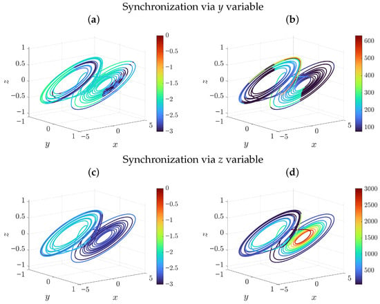
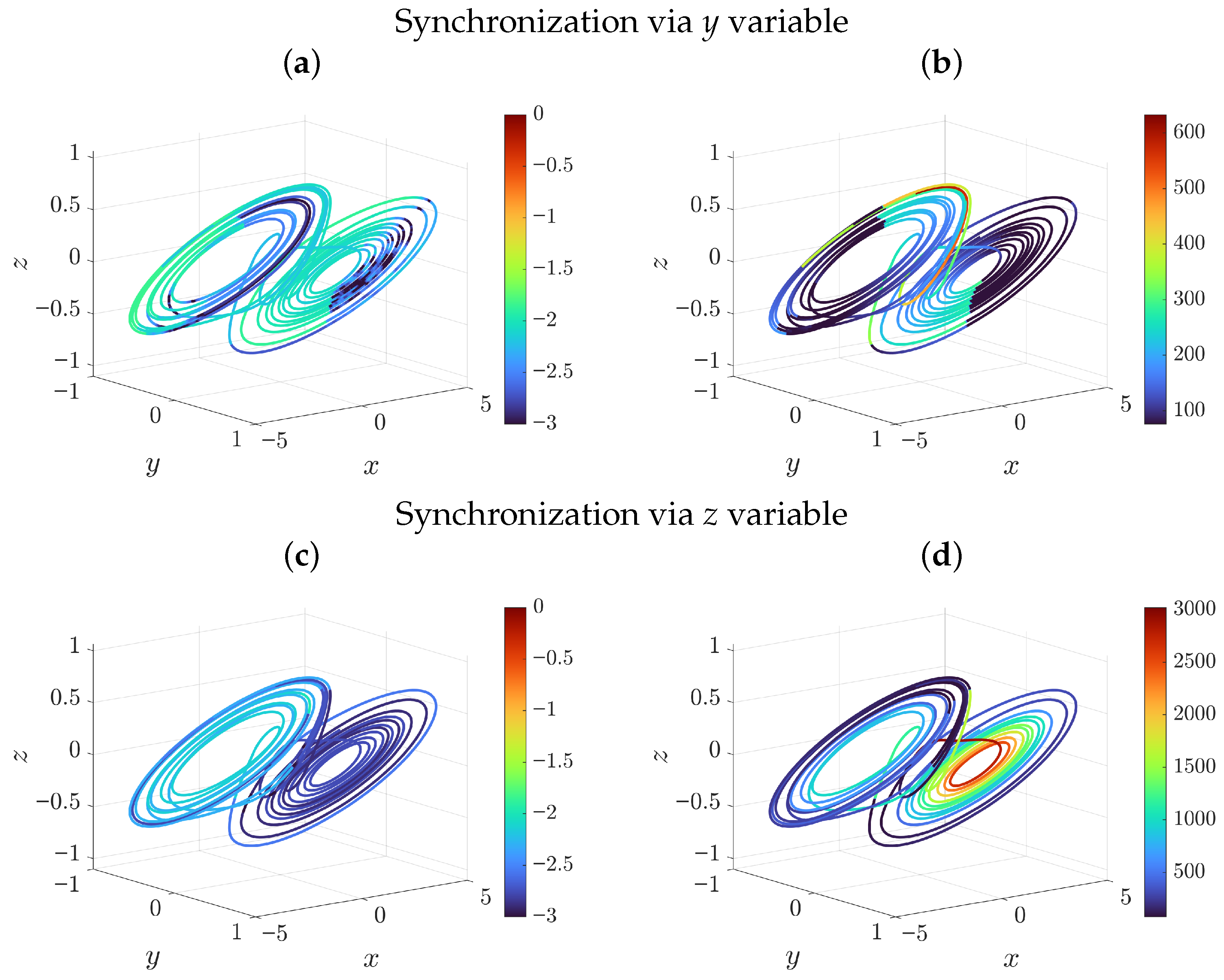
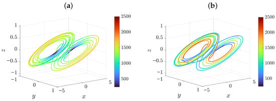
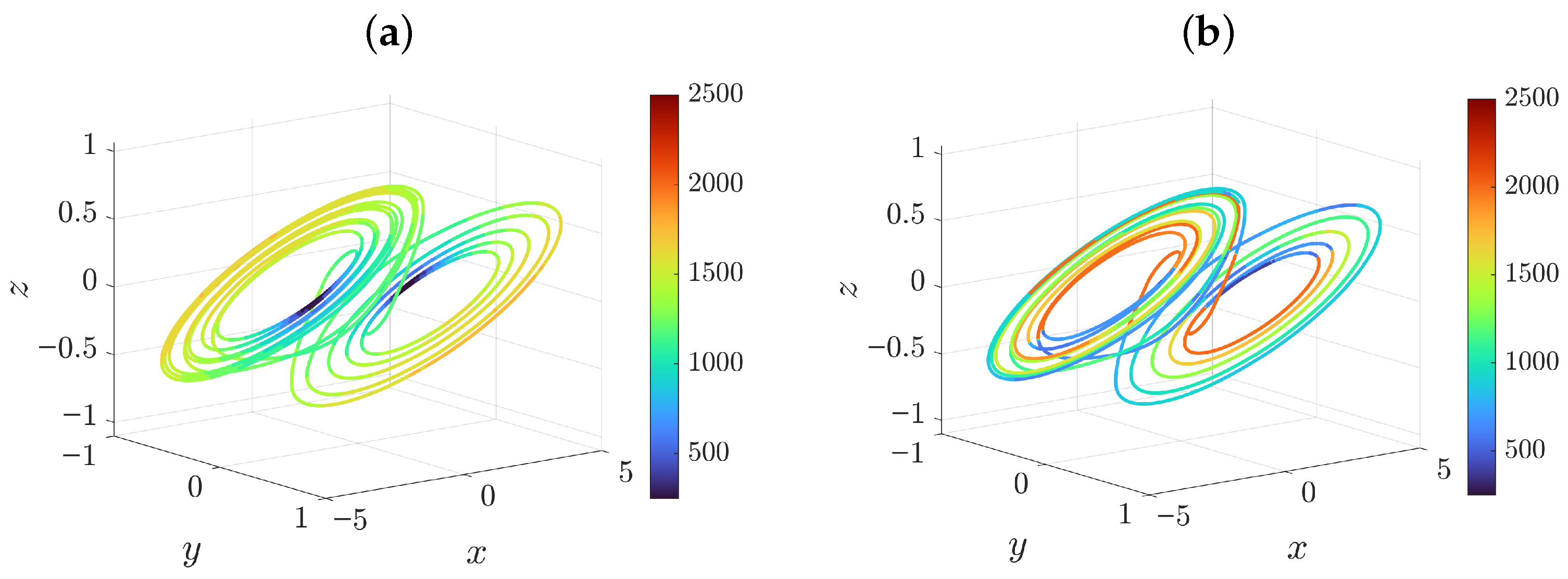
Figure 9 presents the experimental results for synchronization via the y variable (panels a,b) and via the z variable (panels c,d) using the heuristic TRS algorithm. The left panels (a,c) display the Chua circuit attractor with color mapping, indicating the final synchronization error achieved when starting the synchronization process from each point on the trajectory. Blue regions correspond to rapid convergence to errors below $0.01$, while red regions indicate slower but still successful convergence. Gray regions, notably absent in these figures, would indicate failure to synchronize. This proves the robustness of the heuristic approach in real-world conditions.

Figure 9. Heuristic time-reversible synchronization via y variable (a,b) and via z variable (c,d) with real data. The left attractors show in color the level of error that was achieved by starting synchronization from a given point. The right attractors show the required number of data points needed to achieve the target level of synchronization error $\left(0.01\right)$.

The right panels (b,d) of Figure 9 illustrate the most practically significant metric: the number of data points required from the master circuit to achieve the target error level of $0.01$. For y-variable coupling (panel b), the vast majority of starting points require fewer than 600 data samples to achieve complete synchronization, with the most favorable regions requiring as few as 100 samples. This corresponds to merely 1 ms of real-time data acquisition at the $100.251$ kSamples/s rate. For z-variable coupling (panel d), the required data length is somewhat longer, typically ranging from 100 to 500 samples, but still remarkably short compared to conventional methods, and only a small portion of the attractor needed as much as 3000 samples. The color scale reveals that synchronization performance varies smoothly across the attractor, with no abrupt failure regions.

These results demonstrate that the heuristic TRS algorithm can achieve complete synchronization between an analog chaotic circuit and its digital model using only millisecond-duration segments of the chaotic waveform. This capability is particularly valuable for applications such as chaotic communications and neuromorphic sensing, where rapid synchronization from minimal signal samples is essential for real-time operation.

3.2.1. Comparison with Conventional Pecora–Carroll Synchronization

For direct comparison, conventional Pecora–Carroll unidirectional synchronization was evaluated using the same experimental setup. Figure 10 shows the results for synchronization via the x variable (panel a) and via the z variable (panel b). Synchronization via y variable with conventional coupling was omitted as it consistently failed to converge.

Figure 10. Panel (a) illustrates synchronization via x variable and panel (b) via variable z with analog circuit as the master and the digital model as the slave. Color indicates required number of data points needed to achieve the target level of synchronization error $\left(0.01\right)$. $K_x=100,000,K_z=850$.

For x-variable coupling with gain $K_x$ = 100,000 (panel a), Pecora–Carroll synchronization succeeds across substantial portions of the attractor, achieving error levels on the order of ${10}^{-2}$ after no more than 1000 steps (corresponding to 10 ms of real-time data). However, there is a majority of points requiring more than 1000 samples, as yellow and red colors indicate, with a maximal value of 2500. For z-variable coupling with gain $K_z=850$ (panel b), the convergence regions are more fragmented, with large portions of the attractor exhibiting synchronization requiring more than 2000 samples, and only small regions need 500 points and less.

3.2.2. Statistical Analysis of Required Data Length

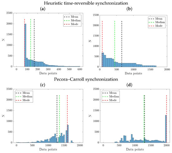
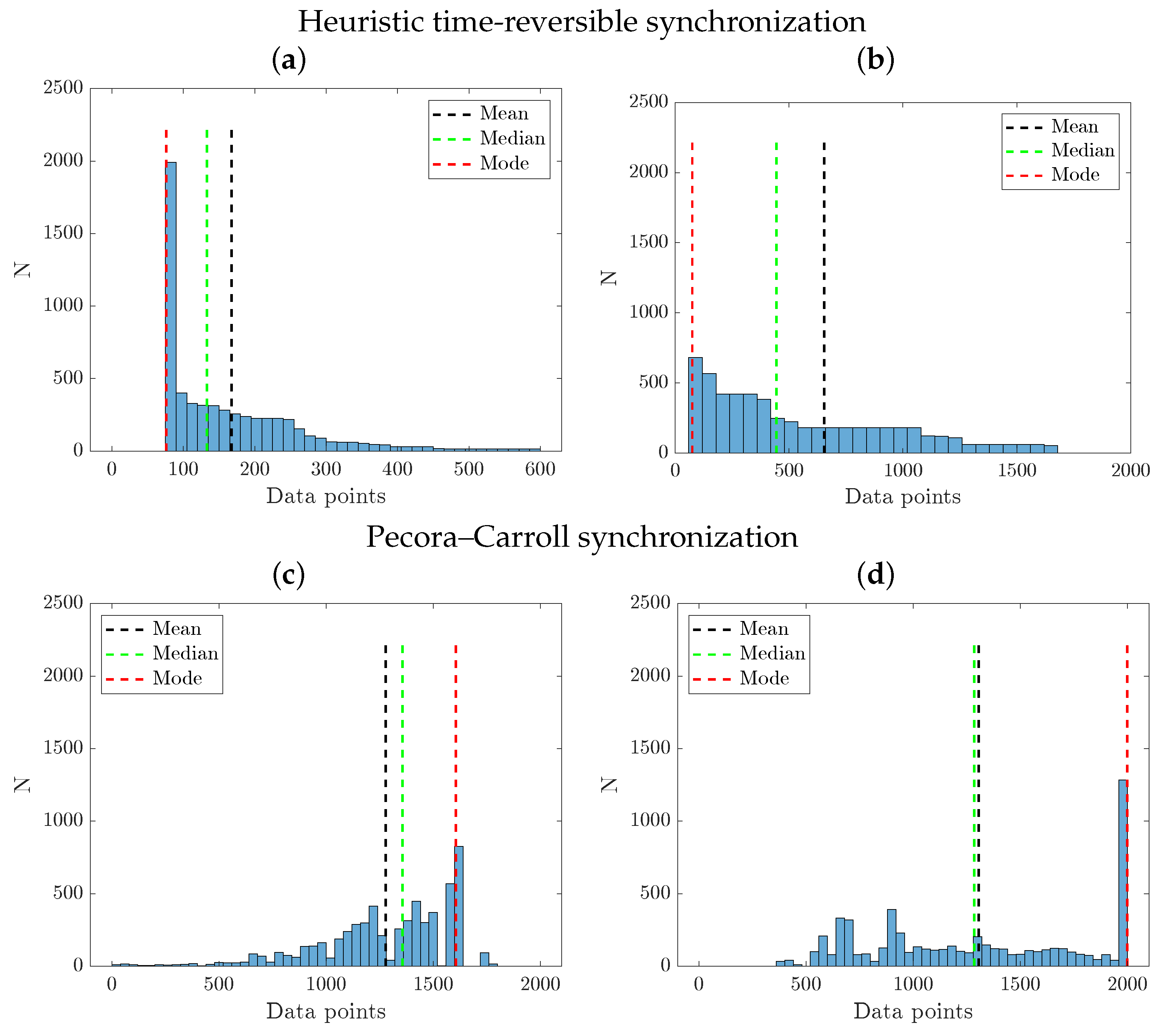
To provide a quantitative comparison between the error convergence rate to a certain preset level of $0.01$, Figure 11 presents histograms of the number of data points required to achieve the target RMS level for both synchronization methods, aggregated over 18,000 randomly selected starting points across the attractor. The results clearly demonstrate the superior efficiency of the heuristic TRS algorithm.

Figure 11. Histograms comparing the number of data points required to achieve synchronization error <0.01 for heuristic time-reversible synchronization with (a) y-coupling and (b) z-coupling and the Pecora–Carroll synchronization with (c) x-coupling and (d) z-coupling. The heuristic TRS algorithm exhibits significantly lower mean, median, and mode values, indicating faster synchronization from fewer data.

For Pecora–Carroll synchronization (c,d), the distribution of required data points is broad and heavily right-skewed. The mean required data length for variable x is 1278 samples (equivalent to $12.78$ ms of real-time data), with a median of 1356 samples, and for variable z, the mean value is 1305 and median is 1284. A substantial fraction of starting points ($33.2\%$) fail to achieve the target error level even after 2000 samples (20 ms), appearing as an accumulation in the rightmost bin of the histogram.

In contrast, the heuristic TRS algorithm (a,b) exhibits a flatter distribution concentrated at low values. The mean required data length is only 160 samples ($1.6$ ms), with a median of 127 samples ($1.27$ ms) for variable y. For variable z, mean is 899 ($8.99$ ms) samples and median is 706 ($7.06$ ms). Remarkably, $92.1\%$ of starting points achieve the target error level within 2000 samples (20 ms), and no starting points require more than 3000 samples. The improvement factors are substantial: in case of z-coupling, the heuristic TRS algorithm achieves a $1.45\times$ reduction in mean required data length and a $1.82\times$ reduction in median required data length compared to conventional Pecora–Carroll synchronization for variable z. Table 6 summarizes the obtained results. In two best cases, when TRS uses y-coupling, and the Pecora–Carroll uses x-coupling, the improvement factors of TRS over Pecora–Carroll synchronization are even more impressive: 8 reduction in mean required data length and $10.1$ in median required data length (see the line “Improvement factor”).

Table 6. Summary of synchronization performance in terms of sample number.

Coupling	P-C	P-C	Heuristic TRS	Heuristic TRS
Variable	Mean	Median	Mean	Median
x	1278	1356	−	−
y	−	−	160	127
z	1305	1284	899	706
Best	1278	1284	160	127
Improvement factor	1×	1×	8.0×	10.1×

These experimental results conclusively validate the practical utility of the proposed heuristic time-reversible synchronization approach. By requiring only millisecond-duration signal segments from the analog circuit, or approximately an order of magnitude less data than the conventional method, the algorithm enables rapid synchronization in applications where data acquisition is limited by hardware constraints or where fast response times are critical.

3.3. Prototype of Edge Intelligent Sensor

The rapid synchronization capabilities of TRS make it well-suited for intelligent edge sensing applications. In this section, we present a proof-of-concept prototype where the modified Chua circuit serves as the core of a capacitive sensor, with capacitor $C_2$ acting as the sensing element. The current implementation focuses on binary classification (nominal vs. 3% perturbed) to validate the detection latency advantage. Extension to continuous parameter estimation, adaptive mismatch tracking, and multi-class discrimination is reserved for future work.

3.3.1. Sensor Principle and Configuration

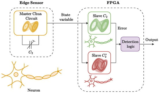
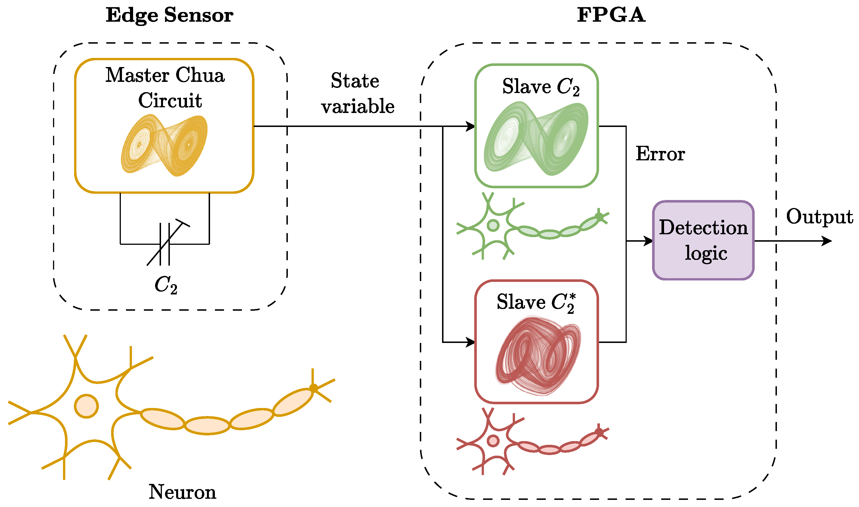
Consider the modified Chua circuit described in Section 2, where capacitor $C_2$ is exposed to the measured physical quantity (e.g., humidity, pressure, or proximity), causing its capacitance to deviate from the nominal value. In this sensor configuration, the physical circuit serves as the master system with an unknown $C_2$ value. Two identical digital slave models are implemented on the FPGA: one with the nominal capacitance value $C_2$ and another with a perturbed value $C_2^{*}=0.97·C_2$, representing a $3\%$ decrease. Both slaves attempt to synchronize with the master using the identical driving signal. Figure 12 illustrates the concept of the proposed sensor.

Figure 12. Schematics of the intelligent edge sensor. The analog circuit acts as a neuron, producing normal activity under normal conditions and abnormal activity in case the sensory element $C_2$ is perturbed under external impact. Two slave digital twins acting as competing observers with the original $C_2$ and the perturbed $C_2^{*}$ capacitors try to synchronize simultaneously. The detection logic block analyses synchronization errors and makes a decision whether the system state belongs to one of two classes of dynamics (normal or abnormal), sending the result to an output.

The choice of coupling variable is arbitrary, but the better the synchronization rate is, the more a particular variable is preferred. For example, y-variable coupling offers superior TRS performance. In this particular application, Pecora–Carroll synchronization, even in the best case of x-variable coupling, loses significantly.

The detection logic is straightforward: when the master system parameters match the nominal slave ($C_2$), it should completely synchronize to the master trajectory, and at a certain time, its synchronization errors should decay below a predefined threshold, e.g., ${ϵ}_{\mathrm{sync}}=0.01$. When the master capacitance deviates ($C_2^{*}=0.97·C_2$), the nominal slave will experience a parameter mismatch, preventing complete synchronization and resulting in a persistently elevated error. On contrary, the perturbed slave, having the parameter $C_2^{*}$ closer to the actual master, would achieve synchronization. The sensor detects a capacitance change when the error of the nominal slave exceeds ${ϵ}_{\mathrm{sync}}$ and the perturbed slave error falls below this threshold.

3.3.2. Synchronization Error Dynamics

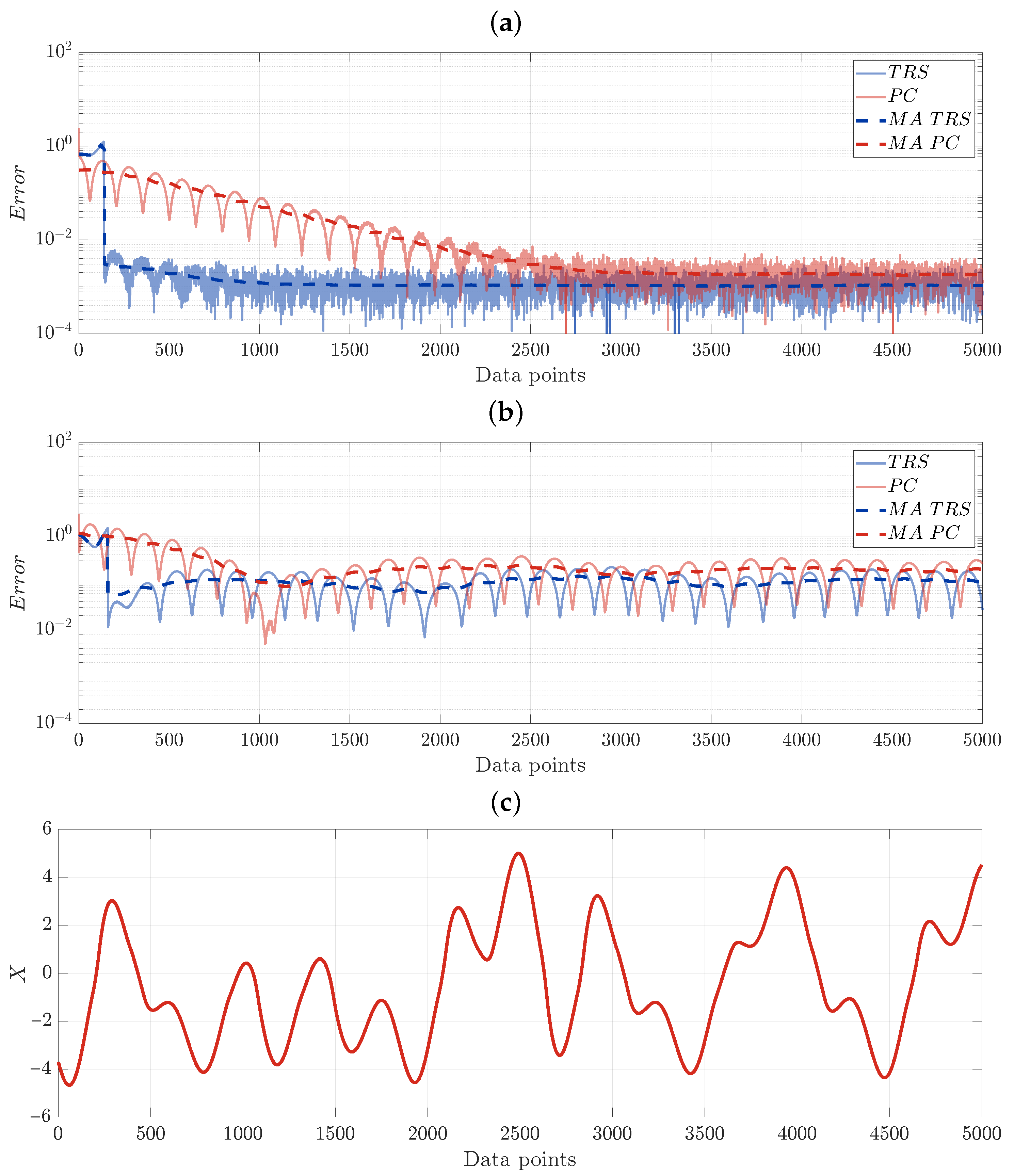
Figure 13 illustrates the error decay dynamics for the two scenarios. Both figures show the instant synchronization error (solid lines) and RMS synchronization error (dashed lines, averaged over 100 samples in a sliding window) as a function of the number of data points received from the master circuit. The experiments were conducted using the same MyRIO-1900 FPGA implementation described in Section 2, with the CD2 integrator and integer-rounded parameters.

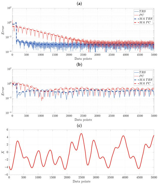
Figure 13. Synchronization error for the heuristic time-reversible synchronization (TRS) algorithm via y-coupling (solid blue) and the Pecora–Carroll (PC) algorithm via variable x-coupling (solid red). Dashed lines represent the moving average (MA). The master and slave systems had identical parameters in panel (a) and different parameters in panel (b) ($C_2^{*}=0.97·C_2$). Panel (c) shows the time evolution of the master system variable x. This experiment illustrates the superiority of the TRS, requiring only approximately a half-pseudo-period (200 data points) in contrast with the PC algorithm, requiring approximately 2000 data points to reach the error below a decision threshold ${ϵ}_{\mathrm{sync}}=0.01$.

Figure 13a presents the case where the master system parameters match the nominal slave. The Pecora–Carroll synchronization (red curve) exhibits monotonic error decay, crossing the detection threshold ${ϵ}_{\mathrm{sync}}=0.01$ after approximately 2000 data points. The TRS (blue curve) allows for abrupt real-time synchronization, requiring only approximately 200 preliminary received data points. While both methods reliably achieve the required error level within the observation window, the time-reversible algorithm demonstrates significantly faster convergence.

Figure 13b shows the scenario where the master capacitance is changed by $3\%$. The nominal slave in both cases now exhibits a persistent synchronization error that remains above ${ϵ}_{\mathrm{sync}}$ even after extended observation. Both errors exhibit oscillations, and it is interesting to note that the TRS still allows for a lower average value than the PC, while complete synchronization is impossible in this case.

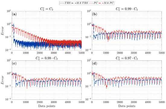
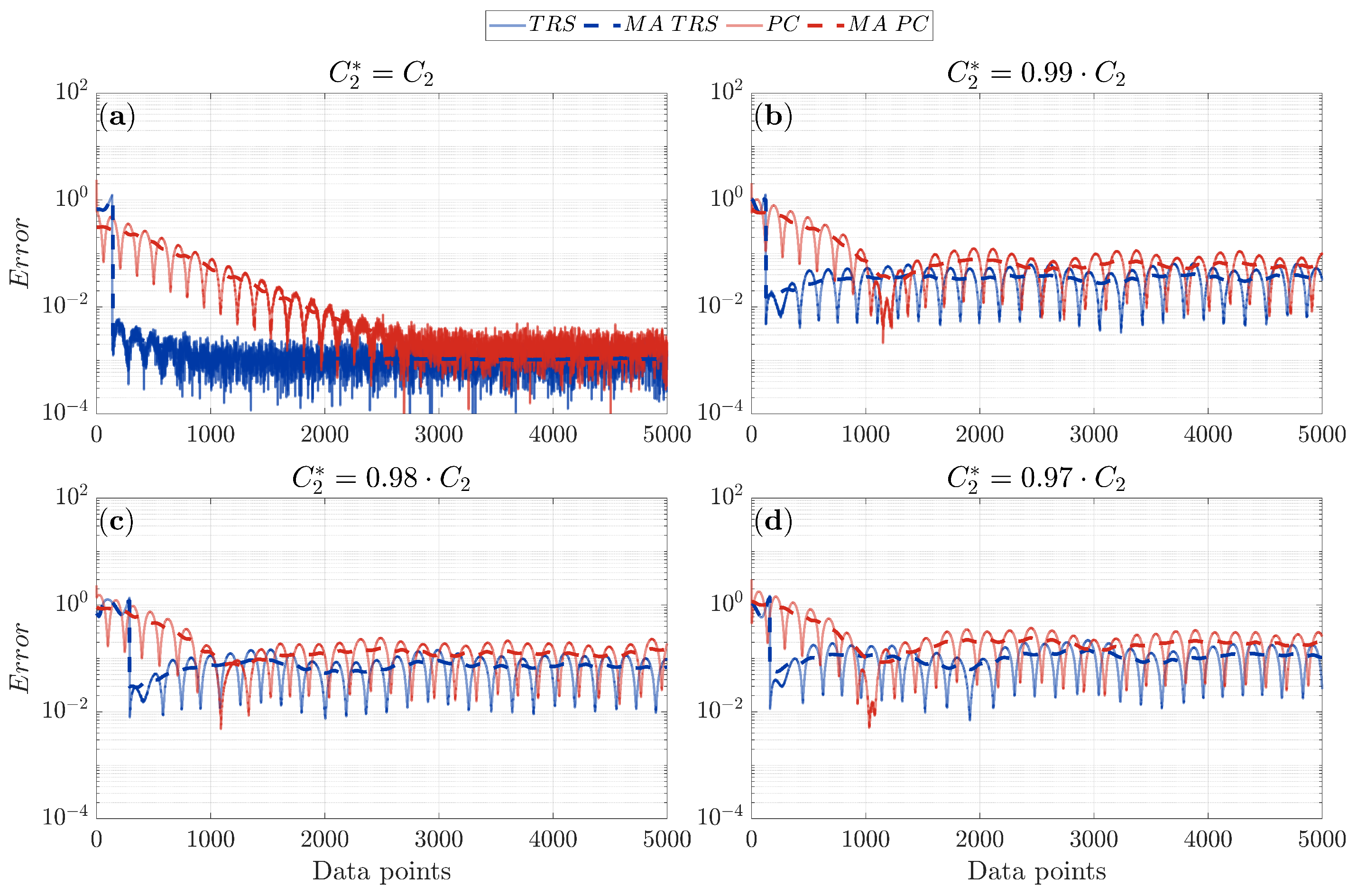
Figure 14 shows the synchronization error dynamics for the heuristic time-reversible synchronization (TRS) algorithm with y-variable coupling (solid blue line) and the classical Pecora–Carroll (PC) algorithm with x-variable coupling (solid red line). Dashed lines denote the moving average (MA). Panel (a) shows the case of identical master and slave system parameters, demonstrating rapid convergence for both methods, with TRS reaching the synchronization threshold significantly faster. Panels (b–d) illustrate algorithm performance under various levels of capacitance mismatch $C_2^{*}\ne C_2$. The results confirm the consistent superiority of TRS: the algorithm not only achieves faster convergence but also exhibits heightened sensitivity to parameter mismatches, which is critical for change-detection applications in sensing scenarios.

Figure 14. Synchronization error for the heuristic time-reversible synchronization (TRS) algorithm via y-coupling (solid blue) and the Pecora–Carroll (PC) algorithm via variable x-coupling (solid red). Dashed lines represent the moving average (MA). The master and slave systems had identical parameters in panel (a); panels (b–d) compare the performance of both algorithms under various capacitance mismatches $C_2^{*}\ne C_2$. This experiment demonstrates the consistent superiority of the TRS algorithm and its greater sensitivity to parameter mismatch.

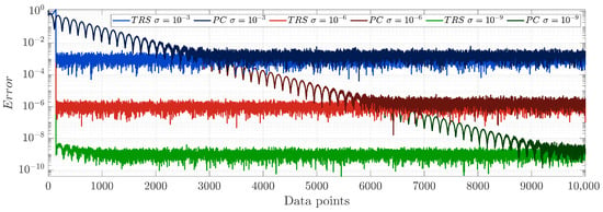
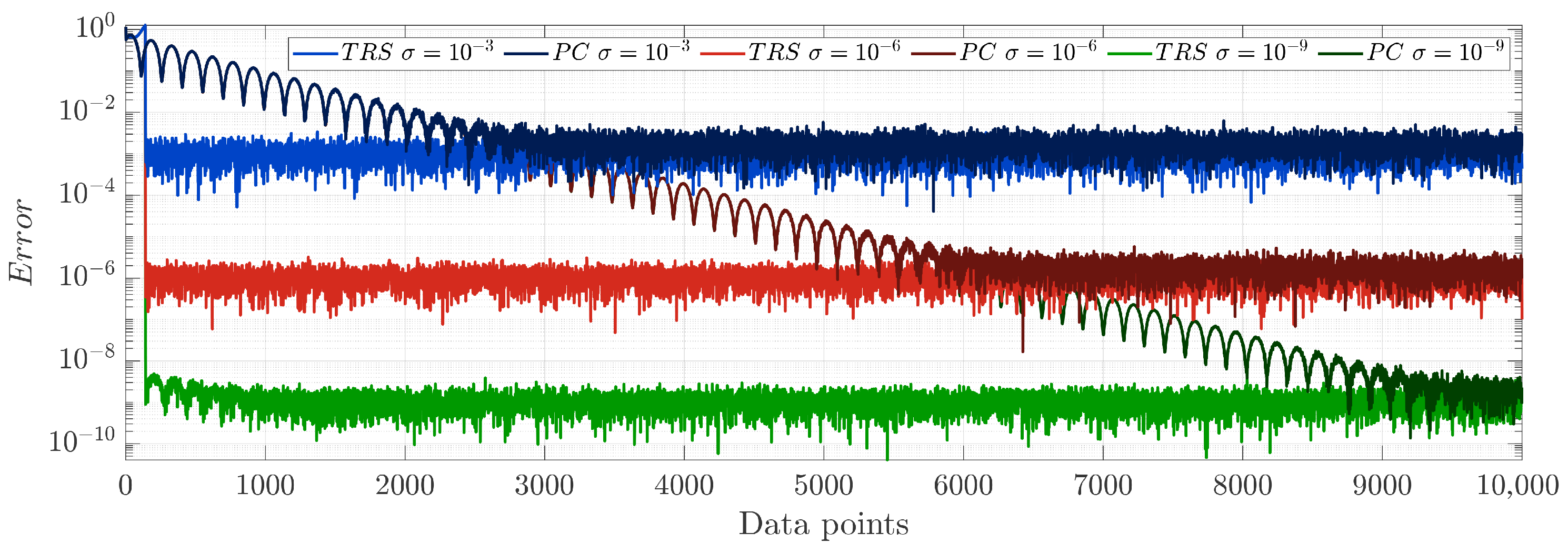
Figure 15 shows the robustness comparison of TRS (y-coupling) and PC (x-coupling) algorithms under additive white Gaussian noise (AWGN) at different intensity levels. The plots show synchronization error vs. the number of received data points for three noise levels: ${10}^{-3},{10}^{-6}$, and ${10}^{-9}$. The TRS algorithm demonstrates superior noise resilience: even in noisy conditions, it maintains the ability to reach the prescribed synchronization error level with fewer iterations compared to the Pecora–Carroll method. This confirms the practical applicability of time-reversible synchronization in real-world environments where signals are inevitably corrupted by noise and highlights the advantage of TRS for developing low-latency intelligent edge sensors.

Figure 15. Synchronization error for the heuristic time-reversible synchronization (TRS) algorithm via y-coupling and the Pecora–Carroll (PC) algorithm via variable x-coupling for different additive white Gaussian noise (AWGN) levels.

3.3.3. Detection Performance and Algorithm Comparison

The sensor detection performance was evaluated by computing the time required to confidently detect a $3\%$ capacitance change, defined as the first data point index n for which the error of one of the slaves (nominal or perturbed) exceeds ${ϵ}_{\mathrm{sync}}$ while the error of another slave remains below ${ϵ}_{\mathrm{sync}}$, with the signal filtered with the moving average of 500 samples to reject false alarms.

Table 7 summarizes the detection performance for both synchronization algorithms, illustrated in Figure 13. For the Pecora–Carroll synchronization, the mean detection time is 893 data samples (median 957, corresponding to $9.57$ ms of real-time data at the 100.251 kSamples/s rate). For time-reversible synchronization, the detection is much faster: a mean of 225 samples (median 195, or $1.95$ ms). This represents a $4\times$ improvement in mean detection speed and a $4.9\times$ improvement in median detection speed.

Table 7. Detection performance for $3\%$ capacitance change using different algorithms.

Algorithm	Mean	Median	Min	Max
	(Samples)	(Samples)	(Samples)	(Samples)
Pecora–Carroll (x-coupling)	893	957	22	2031
Time-reversible (y-coupling)	225	195	75	612
Improvement factor	$4\times$	$4.9\times$	—	—

Note the minimal sample number for the PC algorithm is smaller (22 vs. 75 in case of TRS), which indicates that in some rare cases, favorable initial conditions lead to rapid convergence of the PC algorithm, and TRS requires minimal 75 samples as the length of window required for this algorithm (see Algorithm 2).

4. Discussion and Conclusions

This paper presented a comprehensive investigation of time-reversible synchronization applied to a modified Chua circuit, encompassing the complete pipeline from hardware design through system identification to experimental validation on a MyRIO-1900 FPGA platform.

4.1. Summary of Main Findings

The main contributions are as follows. First, we designed and fabricated a modified Chua circuit with a gyrator-based active inductor replacement and switchable capacitor banks, enabling robust and controllable experimental conditions for sensor emulation. Second, we applied ODERECON system identification to obtain an accurate piecewise-linear model from experimental data, with parameters successfully rounded to integers for FPGA implementation while preserving essential dynamics. Third, we conducted rigorous theoretical analysis of both Pecora–Carroll and time-reversible synchronization, establishing conditions under which synchronization is guaranteed. Fourth, we implemented and experimentally compared conventional Pecora–Carroll coupling with the recently proposed time-reversible synchronization (TRS) algorithm and its heuristic extension (PFHa-TRS), demonstrating superior performance of the adaptive approach. Fifth, we designed and prototyped a capacitive sensor utilizing the developed hardware and software, showing that the heuristic TRS approach provides lower latency and reduced data transmission channel load compared to conventional synchronization.

The experimental results reveal several key novelties. The heuristic TRS algorithm achieves complete synchronization using dramatically fewer data samples than conventional methods: the improvement factor is an order of magnitude reduction in mean and median required data length. Critically, synchronization performance depends strongly on the choice of coupling variable and time direction: while conventional x-coupling performs well, y-coupling fails entirely with conventional methods but succeeds remarkably with TRS, whereas x-coupling with TRS exhibits convergence failures despite its forward-time effectiveness.

The proposed PFHa-TRS algorithm addresses the practical limitation of standard TRS, which fails from substantial regions of the attractor, through adaptive switching to Pecora–Carroll synchronization when errors exceed a threshold, retaining super-exponential convergence in favorable regions while guaranteeing convergence from any initial condition. In a practical capacitive sensor demonstration where $C_2$ serves as the sensing element, a $3\%$ capacitance change was reliably detected within approximately half a pseudo-period of oscillations, with time-reversible synchronization providing a median $4.9\times$ latency improvement over Pecora–Carroll, offering competitive response times.

4.2. Limitations

Despite these promising results, several limitations should be pointed out. While TRS succeeds for two coupling variables, the convergence regions for z-coupling remain significantly more fragmented than for y-coupling, limiting its practical applicability when starting points cannot be controlled. The current study considered only unidirectional coupling through a single state variable. Although this reduces ADC requirements and energy consumption, extension to bidirectional or multivariable coupling schemes remains unexplored. The sensor demonstration considered only a fixed $3\%$ parameter mismatch; real-world sensing applications with continuously varying quantities require adaptive synchronization mechanisms beyond simple detection. Additionally, while the FPGA implementation achieved real-time performance, the CD2 integrator and iterative TRS algorithm impose computational demands that may exceed the capabilities of ultra-low-power microcontrollers or prove challenging for synchronization with high-frequency oscillators.

Additionally, the current sensing demonstration validates detection under a fixed 3% parameter mismatch. Real-world applications with continuously varying quantities or varying noise floors will require adaptive synchronization thresholds and multi-slave observer architectures. Furthermore, while the current PCB prototype demonstrated reliable chaotic dynamics, future hardware iterations will employ professional fabrication services to further suppress parasitic coupling, reduce thermal drift, and improve long-term reproducibility in industrial environments.

4.3. Concluding Remarks and Future Work

This paper demonstrates that time-reversible synchronization, particularly in its heuristic extension (PFHa-TRS), offers a practically viable approach for achieving rapid and reliable synchronization between analog chaotic circuits and digital models. The experimental validation on the modified Chua circuit confirms theoretical predictions of super-exponential convergence and reveals important variable-dependent behavior. The capacitive sensor demonstration illustrates how these properties can be used in practical applications, achieving millisecond-scale detection with simple hardware. Time-reversible synchronization, despite its sensitivity to initial conditions in pure form, can be made practically robust through heuristic hybridization with conventional methods, allowing for fast response times and minimal data requirements in practical applications.

Future work will focus on three directions: developing a rigorous mathematical framework to predict convergence regions based on local Lyapunov spectra, extending TRS principles to bidirectional and network synchronization for distributed sensing applications, and implementing adaptive time-reversible synchronization to further improve efficiency in real-time parameter estimation scenarios.

References

- Pecora, L.M.; Carroll, T.L. Synchronization in chaotic systems. Phys. Rev. Lett. 1990, 64, 821. [Google Scholar] [CrossRef] [Scilit]
- Cuomo, K.M.; Oppenheim, A.V. Circuit implementation of synchronized chaos with applications to communications. Phys. Rev. Lett. 1993, 71, 65. [Google Scholar] [CrossRef] [Scilit]
- Boccaletti, S.; Kurths, J.; Osipov, G.; Valladares, D.; Zhou, C. The synchronization of chaotic systems. Phys. Rep. 2002, 366, 1–101. [Google Scholar] [CrossRef] [Scilit]
- Pecora, L.M.; Carroll, T.L. Synchronization of chaotic systems. Chaos Interdiscip. J. Nonlinear Sci. 2015, 25, 097611. [Google Scholar] [CrossRef] [Scilit]
- Kabziński, J.; Mosiołek, P. Adaptive, observer-based synchronization of different chaotic systems. Appl. Sci. 2022, 12, 3394. [Google Scholar] [CrossRef] [Scilit]
- Xing, Y.; Dong, W.; Zeng, J.; Guo, P.; Zhang, J.; Ding, Q. Study of generalized chaotic synchronization method incorporating error-feedback coefficients. Entropy 2023, 25, 818. [Google Scholar] [CrossRef] [Scilit]
- Yan, J.J.; Lin, J.S.; Liao, T.L. Synchronization of a modified Chua’s circuit system via adaptive sliding mode control. Chaos Solitons Fractals 2008, 36, 45–52. [Google Scholar] [CrossRef] [Scilit]
- Liu, Q.; Yan, H.; Zhang, H.; Zhan, X.; Shi, K. Intermittent exponential synchronization for memristor-based neural networks with inertial items and mixed time-varying delays. IEEE Trans. Syst. Man, Cybern. Syst. 2022, 53, 2925–2937. [Google Scholar] [CrossRef] [Scilit]
- Liu, Y.; Li, H.; Lu, R.; Zuo, Z.; Li, X. An overview of finite/fixed-time control and its application in engineering systems. IEEE/CAA J. Autom. Sin. 2022, 9, 2106–2120. [Google Scholar] [CrossRef] [Scilit]
- Karimov, T.; Druzhina, O.; Karimov, A.; Tutueva, A.; Ostrovskii, V.; Rybin, V.; Butusov, D. Single-coil metal detector based on spiking chaotic oscillator. Nonlinear Dyn. 2022, 107, 1295–1312. [Google Scholar] [CrossRef] [Scilit]
- Silva, I.G.; Korneta, W.; Stavrinides, S.G.; Picos, R.; Chua, L.O. Observation of stochastic resonance for weak periodic magnetic field signal using a chaotic system. Commun. Nonlinear Sci. Numer. Simul. 2021, 94, 105558. [Google Scholar] [CrossRef] [Scilit]
- Babajans, R.; Cirjulina, D.; Tjukovs, S.; Becchi, S.; Secco, J.; Vovchuk, D.; Kolosovs, D.; Pikulins, D. Chaos-Based Dynamical Parameter Estimation for Physical Layer Authentication in Wireless IoT Networks. Electronics 2026, 15, 748. [Google Scholar] [CrossRef] [Scilit]
- Zhao, H.; Njilla, L. Hardware assisted chaos based iot authentication. In Proceedings of the 2019 IEEE 16th International Conference on Networking, Sensing and Control (ICNSC); IEEE: New York, NY, USA, 2019; pp. 169–174. [Google Scholar]
- Yu, S.; Chen, W.; Poor, H.V. Real-time monitoring of chaotic systems with known dynamical equations. IEEE Trans. Signal Process. 2024, 72, 1251–1268. [Google Scholar] [CrossRef] [Scilit]
- Kent, R.M.; Barbosa, W.A.; Gauthier, D.J. Controlling chaos using edge computing hardware. Nat. Commun. 2024, 15, 3886. [Google Scholar] [CrossRef] [Scilit] [PubMed]
- Hudson, J.; Jolly, M. Numerical efficacy study of data assimilation for the 2D magnetohydrodynamic equations. J. Comput. Dyn. 2019, 6, 131–145. [Google Scholar] [CrossRef] [Scilit]
- Chu, Y.; Li, X.; Han, X. Exponential synchronization of complex networks with unmeasured coupling delays via impulsive observer and impulsive control. Appl. Math. Comput. 2024, 479, 128843. [Google Scholar] [CrossRef] [Scilit]
- Yan, L.; Dai, H. Event-triggered synchronization for second-order linear systems in complex dynamical network with time-varying topology. Int. J. Control. Autom. Syst. 2024, 22, 1779–1790. [Google Scholar] [CrossRef] [Scilit]
- Chen, D.; Li, S.; Wu, Q. Rejecting chaotic disturbances using a super-exponential-zeroing neurodynamic approach for synchronization of chaotic sensor systems. Sensors 2018, 19, 74. [Google Scholar] [CrossRef] [Scilit]
- Xiao, L.; Zhao, L.; Jin, J. Preset-time convergence fuzzy zeroing neural network for chaotic system synchronization: FPGA validation and secure communication applications. Sensors 2025, 25, 5394. [Google Scholar] [CrossRef] [Scilit] [PubMed]
- Tong, Y.; Liu, J.; Zhou, H.; Ju, Z.; Zhang, X. Adaptive tracking control of robotic manipulators with unknown kinematics and uncertain dynamics. IEEE Trans. Autom. Sci. Eng. 2023, 21, 5252–5269. [Google Scholar] [CrossRef] [Scilit]
- Arcak, M. Circle-criterion observers and their feedback applications: An overview. In Current Trends in Nonlinear Systems and Control: In Honor of Petar Kokotović and Turi Nicosia; Springer: Berlin/Heidelberg, Germany, 2006; pp. 3–14. [Google Scholar]
- Li, D.; Zheng, Z.; Cui, Y.; Chen, M.; Zou, L. Prescribed-time trajectory tracking control for manipulators based on disturbance observers. Nonlinear Dyn. 2025, 113, 29461–29474. [Google Scholar] [CrossRef] [Scilit]
- Luo, D.; Wang, Y.; Song, Y. Practical prescribed time tracking control with bounded time-varying gain under non-vanishing uncertainties. IEEE/CAA J. Autom. Sin. 2024, 11, 219–230. [Google Scholar] [CrossRef] [Scilit]
- Song, Y.; Ye, H.; Lewis, F.L. Prescribed-time control and its latest developments. IEEE Trans. Syst. Man Cybern. Syst. 2023, 53, 4102–4116. [Google Scholar] [CrossRef] [Scilit]
- Butusov, D.; Rybin, V.; Karimov, A. Fast time-reversible synchronization of chaotic systems. Phys. Rev. E 2025, 111, 014213. [Google Scholar] [CrossRef] [Scilit]
- Butcher, J.; Hill, A.; Norton, T. Symmetric general linear methods. BIT Numer. Math. 2016, 56, 1189–1212. [Google Scholar] [CrossRef] [Scilit]
- Babkin, I.; Rybin, V.; Karimov, A.; Butusov, D. Practically feasible heuristic algorithm for time-reversible synchronization of chaotic oscillators. Chaos Solitons Fractals 2026, 202, 117470. [Google Scholar] [CrossRef] [Scilit]
- Chua, L.O.; Itoh, M.; Kocarev, L.; Eckert, K. Chaos synchronization in Chua’s circuit. J. Circuits Syst. Comput. 1993, 3, 93–108. [Google Scholar] [CrossRef] [Scilit]
- Iliuk, I.; Balthazar, J.M.; Tusset, A.M.; Felix, J.L.P.; de Pontes, B.R., Jr. On non-ideal and chaotic energy harvester behavior. Differ. Equ. Dyn. Syst. 2013, 21, 93–104. [Google Scholar] [CrossRef] [Scilit]
- Karimov, A.; Rybin, V.; Kopets, E.; Karimov, T.; Nepomuceno, E.; Butusov, D. Identifying empirical equations of chaotic circuit from data. Nonlinear Dyn. 2023, 111, 871–886. [Google Scholar] [CrossRef] [Scilit]
- Matsumoto, T. A chaotic attractor from Chua’s circuit. IEEE Trans. Circuits Syst. 1984, 31, 1055–1058. [Google Scholar] [CrossRef] [Scilit]
- Pikovskii, A.; Rabinovich, M. A simple autogenerator with stochastic behaviour. Rep. Ussr Acad. Sci. 1978, 239, 2. [Google Scholar]
- Duan, Z.; Zhang, X.; He, S.; Yu, X.; Xiong, P.; Chen, J.; Wang, Q. Implementation of a fully integrated memristive Chua’s chaotic circuit with a voltage-controlled oscillator. Integration 2024, 99, 102258. [Google Scholar] [CrossRef] [Scilit]
- Chen, M.; Yu, J.; Yu, Q.; Li, C.; Bao, B. A memristive diode bridge-based canonical Chua’s circuit. Entropy 2014, 16, 6464–6476. [Google Scholar] [CrossRef] [Scilit]
- Kera, H.; Hasegawa, Y. Noise-tolerant algebraic method for reconstruction of nonlinear dynamical systems. Nonlinear Dyn. 2016, 85, 675–692. [Google Scholar] [CrossRef] [Scilit]
- Rosafalco, L.; Conti, P.; Manzoni, A.; Mariani, S.; Frangi, A. Online learning in bifurcating dynamic systems via SINDy and Kalman filtering. Nonlinear Dyn. 2025, 113, 14201–14221. [Google Scholar] [CrossRef] [Scilit]
- Liu, D.; Sopasakis, A. Enhancing sparse identification of nonlinear dynamics with Earth-Mover distance and group similarity. Chaos Interdiscip. J. Nonlinear Sci. 2025, 35, 033139. [Google Scholar] [CrossRef] [Scilit]
- Chen, Z.; Zhu, W.; Bian, H.; Yang, G. Data-driven system identification for piecewise dynamical systems via Sparse Identification Neural Ordinary Differential Equations. Chaos Solitons Fractals 2025, 200, 117028. [Google Scholar] [CrossRef] [Scilit]
Disclaimer/Publisher’s Note: The statements, opinions and data contained in all publications are solely those of the individual author(s) and contributor(s) and not of MDPI and/or the editor(s). MDPI and/or the editor(s) disclaim responsibility for any injury to people or property resulting from any ideas, methods, instructions or products referred to in the content. |
© 2026 by the authors. Licensee MDPI, Basel, Switzerland. This article is an open access article distributed under the terms and conditions of the Creative Commons Attribution (CC BY) license.