Large Deviations for the Supremum of Partial Sums of Non-Independent and Non-Identically Distributed Random Variables

Abstract

In this paper, we establish the large deviation principle for the supremum of partial sums of a sequence of non-independent and non-identically distributed random variables. Let $\{X_n:n\ge 1\}$ be a sequence of random variables with the same negative mean, and denote $S_n={\sum }_{i=1}^n{X}_i$, $S_0=0$, and assume that the limit $\mathsf{\Lambda }\left(\theta \right)={lim}_{n\to \infty }{\displaystyle \frac{1}{n}}{\mathsf{\Lambda }}_n\left(\theta \right)$ of the logarithmic moment generating functions ${\mathsf{\Lambda }}_n\left(\theta \right)=logE\left[e^{\theta S_n}\right]$ exists and is essentially smooth and lower semi-continuous. We prove that the sequence $\left\{{\displaystyle \frac{1}{l}}{sup}_{n\ge 0}{S}_n:l\ge 1\right\}$ satisfies the large deviation principle on $\mathbb{R}$ and provide the exact form of its rate function. As a consequence, we obtain the large deviation principle for the supremum of sums formed by combining independent and identically distributed components with correlated components. As applications, we analyze the first-order autoregressive process and the Poisson–Gaussian mixture case and derive exact expressions for the corresponding rate functions and asymptotic estimates for the decay of tail probabilities.

1. Introduction

Let $(\mathsf{\Omega },\mathcal{F},P)$ be a probability space, and consider a sequence of real-valued random variables $\{X_n:n\ge 1\}$. Define the partial sums of this random sequence as $S_n:={\sum }_{i=1}^n{X}_i$. Large deviation theory is a significant branch of limit theory in probability, whose core content lies in describing the asymptotic property that the probability of rare events decays exponentially. Cramér’s pioneering work [1] laid the foundation for large deviation theory. Under finite moment conditions (i.e., the Cramér condition: if there exists $\lambda >0$ such that $E{e}^{\lambda |X_1|}<\infty$), Cramér proved that the sequence $\left\{{\displaystyle \frac{1}{n}}{S}_n:n\ge 1\right\}$ satisfies the large deviation principle with rate function ${\mathsf{\Lambda }}^{*}\left(x\right)={sup}_{\theta \in \mathbb{R}}\{\theta x-\mathsf{\Lambda }\left(\theta \right)\}$, where $\mathsf{\Lambda }\left(\theta \right)=logE\left[e^{\theta X_1}\right]$ is the logarithmic moment generating function. Specifically, for any measurable set $B\subset \mathbb{R}$, the following holds:

$$\begin{array}{cc}\hfill -\underset{x\in B^{\circ }}{inf}{\mathsf{\Lambda }}^{*}\left(x\right)& \le \underset{n\to \infty }{lim\; inf}{\displaystyle \frac{1}{n}}logP\left({\displaystyle \frac{S_n}{n}}\in B\right)\hfill \\ \hfill & \le \underset{n\to \infty }{lim\; sup}{\displaystyle \frac{1}{n}}logP\left({\displaystyle \frac{S_n}{n}}\in B\right)\le -\underset{x\in \overline{B}}{inf}{\mathsf{\Lambda }}^{*}\left(x\right),\hfill \end{array}$$

where $B^{\circ }$ denotes the interior of B and $\overline{B}$ denotes its closure.

Following Cramér’s pioneering work, large deviation theory for partial sums of random variables has been systematically developed. Nagaev [2] first moved beyond the classical reliance on the Cramér condition and laid the foundation for the asymptotic theory of partial sums under heavy-tailed distributions. Subsequently, Nagaev [3] extended the large deviation bounds for partial sums to independent and non-identically distributed sequences by establishing general deviation inequalities. To describe more complex heterogeneity, Kiesel and Stadtmüller [4] as well as Gantert et al. [5] extended the research to weighted partial sums and stretched exponential tails under independent and non-identically distributed cases, respectively, thus broadening the applicability of large deviation theory for partial sums.

With the development of society, research attention was shifted toward large deviations for extreme statistics of partial sums. Duffield and O’Connell [6] established a large deviation framework for workload processes with certain scaling properties and their supremum, deriving asymptotic estimates for the tail probability of the supremum of workload process. Korshunov [7] provided a landmark contribution by unifying the asymptotic behavior of tail probabilities for the supremum of random walks with negative mean under both light- and heavy-tailed scenarios. Kozlov [8] and Shklyaev [9] established large deviation principles for the maximum of partial sums of non-negative independent random variable sequences and general independent random variable sequences, respectively, under the Cramér condition. With the deepening of research, scholars began to focus on asymptotic behaviors under non-independent cases. Bryc and Dembo [10] proved that the empirical measure of strongly mixing ($\alpha$-mixing) stationary processes satisfies a large deviation principle. For dependent sequences, Choe and Shroff [11] employed extreme value theory to study the upper tail asymptotics for the supremum of stationary increment Gaussian processes. Fan, Grama, and Liu [12] extended large deviation research for the maximum to dependent martingale difference sequences with conditional subexponential moments. Recently, Lu and Cai [13] studied precise large deviations for sums of dependent random variables under the framework with a subexponential tail and characterized the asymptotic equivalence form of tail probabilities in generalized dependence structures, while Matula [14] studied exact limit laws for extreme statistics of non-independent and non-identically distributed Pareto-type random variables.

However, existing research in this area has predominantly relied on assumptions of independence, identical distribution, martingale difference structures, or some special distributions. This limitation restricts the application of the theory in modeling real complex systems, such as stochastic processes in communication networks and queuing systems, which are often neither independent nor identically distributed. This paper seeks to advance this theoretical aspect by studying the large deviation principle for the supremum of partial sums of a sequence of non-independent and non-identically distributed random variables. Under the assumption that the limit of the logarithmic moment generating function $\mathsf{\Lambda }\left(\theta \right)={lim}_{n\to \infty }{\displaystyle \frac{1}{n}}logE\left[e^{\theta S_n}\right]$ exists and is essentially smooth and lower semi-continuous, we establish the large deviation principle for the sequence $\left\{{\displaystyle \frac{1}{l}}{sup}_{n\ge 0}{S}_n:l\ge 1\right\}$, and obtain an exact expression for its rate function. As a theoretical extension, the results are generalized to sequences formed by sums of independent, identically distributed components and correlated components, thereby providing a framework for analyzing a wider class of dependence structures. Finally, the theory is applied to two concrete models: a first-order autoregressive process and a Poisson–Gaussian mixture case. In each case, we provide exact expressions for the corresponding rate function and obtain asymptotic estimates for the tail probabilities.

The structure of this paper is organized as follows. We firstly introduce the basic concepts and preliminary theorems of large deviation theory in Section 2. Then, the main results and their corollaries are presented in Section 3. The detailed proofs of the main theorems are provided in Section 4, followed by the proofs of the lemmas in Section 5. Finally, the applications of the main theorems are demonstrated through two examples in Section 6.

2. Preliminaries

Before stating the main results and proofs, we first introduce some basic definitions and theorems that can be found in references [15,16].

Definition 1

(Rate Function). (1) A function $I:\mathcal{X}\to [0,\infty ]$ is called a rate function if it is non-negative and lower semi-continuous, i.e., for $\alpha \in \mathbb{R}$, the level set $\{x:I(x)\le \alpha \}$ is closed. (2) A rate function I is called a good rate function if its level sets are compact.

Definition 2

(Essential Smoothness). A function $f:\mathbb{R}\to \mathbb{R}\cup \{\infty \}$ is called essentially smooth if the interior of its effective domain is non-empty, f is differentiable in the interior of its effective domain, and f is steep, namely, for any sequence $\{{\theta }_n:n\ge 1\}$ converging to a boundary point of the effective domain, ${lim}_{n\to \infty }\left|f^{\prime }\left({\theta }_n\right)\right|=+\infty$.

Definition 3

(Large Deviation Principle). Let $\{X_n:n\ge 1\}$ be a sequence of random variables and I be a rate function. We say that $\{X_n:n\ge 1\}$ satisfies the large deviation principle in $\mathbb{R}$ with rate function I if for any closed set $F\subset \mathbb{R}$,

$$\underset{n\to \infty }{lim\; sup}{\displaystyle \frac{1}{n}}logP(X_n\in F)\le -\underset{x\in F}{inf}I\left(x\right),$$

and for any open set $G\subset \mathbb{R}$,

$$\underset{n\to \infty }{lim\; inf}{\displaystyle \frac{1}{n}}logP(X_n\in G)\ge -\underset{x\in G}{inf}I\left(x\right).$$

Inequality (1) is called the large deviations upper bound, and inequality (2) is called the large deviations lower bound.

Theorem 1

(Gärtner–Ellis Theorem). Let $\{X_n:n\ge 1\}$ be a sequence of random variables, $S_n={\sum }_{i=1}^n{X}_i$. If for all $\theta \in \mathbb{R}$, the limit

$$\mathsf{\Lambda }\left(\theta \right)=\underset{n\to \infty }{lim}{\displaystyle \frac{1}{n}}logE\left(e^{\theta S_n}\right)$$

exists as an extended real number, and if $\mathsf{\Lambda }\left(\theta \right)$ is finite in a neighborhood of the origin, essentially smooth, and lower semi-continuous, then the random variable sequence $\left\{{\displaystyle \frac{S_n}{n}}:n\ge 1\right\}$ satisfies the large deviation principle on $\mathbb{R}$ with good rate function ${\mathsf{\Lambda }}^{*}$.

Theorem 2

(Convergence of Derivatives of Convex Functions). Let $\{f_n:n\ge 1\}$ be a sequence of convex functions $f_n:\mathbb{R}\to \mathbb{R}\cup \{\infty \}$, converging pointwise to a function f (f is necessarily convex). Suppose that for each n, $f_n$ is finite and differentiable in a neighbourhood of the origin, and that $f_n^{\prime }\left(0\right)={\mu }_n$. If f is differentiable at the origin and if ${\mu }_n\to \mu$, then $f^{\prime }\left(0\right)=\mu$.

Theorem 3

(Properties of logarithmic moment generating function for an arbitrary real-valued random variable). Let X be a real-valued random variable, and define

$${\mathsf{\Lambda }}_1\left(\theta \right):=log\mathbb{E}\left[e^{\theta X}\right],D_{{\mathsf{\Lambda }}_1}:=\{\theta \in \mathbb{R}:\mathbb{E}\left[e^{\theta X}\right]<\infty \}.$$

Then:

(i)   

${\mathsf{\Lambda }}_1$ is convex and lower semi-continuous, and ${\mathsf{\Lambda }}_1\left(0\right)=0$;

(ii) 

${\mathsf{\Lambda }}_1$ is differentiable on $\mathrm{int}\left(D_{{\mathsf{\Lambda }}_1}\right)$, with

$${\mathsf{\Lambda }}_1^{\prime }\left(\theta \right)={\displaystyle \frac{\mathbb{E}\left[X{e}^{\theta X}\right]}{\mathbb{E}\left[e^{\theta X}\right]}};$$

(iii) 

if ${\mathsf{\Lambda }}_1$ is finite in a neighborhood of 0, then $\mathbb{E}\left[X\right]$ is finite and

$${\mathsf{\Lambda }}_1^{\prime }\left(0\right)=\mathbb{E}\left[X\right].$$

Theorem 4

(Properties of Convex Conjugate Function). Let Λ be the logarithmic moment generating function of a real-valued random variable X, and ${\mathsf{\Lambda }}^{*}$ be its convex conjugate. Then

1.

${\mathsf{\Lambda }}^{*}$ is non-negative, convex, and lower semi-continuous;

2.

${\left({\mathsf{\Lambda }}^{*}\right)}^{*}=\mathsf{\Lambda }$.

If $\mathsf{\Lambda }\left(\theta \right)$ is finite in a neighborhood of zero, then

1. 

$\mu =E\left(X\right)$ is finite and equals to ${\mathsf{\Lambda }}^{\prime }\left(0\right)$;

2. 

${\mathsf{\Lambda }}^{*}\left(\mu \right)=0$;

3. 

${\mathsf{\Lambda }}^{*}$ is decreasing on $(-\infty ,\mu ]$ and increasing on $[\mu ,\infty )$.

3. Main Results

Let $\{X_n:n\ge 1\}$ be a sequence of random variables, and denote $S_n:={\displaystyle \sum _{i=1}^n}{X}_i$. We shall investigate the large deviation principle for the sequence $\{{\displaystyle \frac{1}{l}}\underset{n\ge 0}{sup}{S}_n:l\ge 1\}$. The main results of this paper are as follows.

Theorem 5.

Let $\{X_n:n\ge 1\}$ be a sequence of random variables, $\forall n\ge 1$, $E\left(X_1\right)=E\left(X_2\right)=\cdots =E\left(X_n\right)$, and $E\left(X_1\right)<0$. Let $S_n={\sum }_{i=1}^n{X}_i$, $S_0=0$, ${\mathsf{\Lambda }}_n\left(\theta \right)=log\mathbb{E}\left[e^{\theta S_n}\right]$. Suppose that the limit $\mathsf{\Lambda }\left(\theta \right)={lim}_{n\to \infty }{\displaystyle \frac{1}{n}}{\mathsf{\Lambda }}_n\left(\theta \right)$ exists in $\mathbb{R}\cup \{\infty \}$ for each $\theta \in \mathbb{R}$, and that $\mathsf{\Lambda }\left(\theta \right)$ is essentially smooth, lower semi-continuous, and finite in a neighborhood of $\theta =0$; when $\mathsf{\Lambda }\left(\theta \right)<0$, ${\mathsf{\Lambda }}_n\left(\theta \right)$ is finite for each n. Then for any closed set F in $\mathbb{R}$, we have

$$\underset{l\to \infty }{lim\; sup}{\displaystyle \frac{1}{l}}logP\left({\displaystyle \frac{1}{l}}\underset{n\ge 0}{sup}{S}_n\in F\right)\le -\underset{x\in F}{inf}I\left(x\right),$$

and for any open set G in $\mathbb{R}$, we have

$$\underset{l\to \infty }{lim\; inf}{\displaystyle \frac{1}{l}}logP\left({\displaystyle \frac{1}{l}}\underset{n\ge 0}{sup}{S}_n\in G\right)\ge -\underset{x\in G}{inf}I\left(x\right),$$

where $I\left(x\right)={inf}_{t\in {\mathbb{R}}^{+}}t{\mathsf{\Lambda }}^{*}\left({\displaystyle \frac{x}{t}}\right)=xsup\{\theta >0:\mathsf{\Lambda }\left(\theta \right)<0\}$.

Corollary 1.

Let $Y_n=A_n+X_n$, where $\{A_n:n\ge 1\}$ is an independent identically distributed random variable sequence, $\{X_n:n\ge 1\}$ is a non-independent random variable sequence, $\{A_n:n\ge 1\}$ and $\{X_n:n\ge 1\}$ are independent, and $E\left[Y_1\right]=E\left[Y_2\right]=\cdots =E\left[Y_n\right]<0$.

Define partial sums and logarithmic moment generating functions:

$$S_n^Y=\sum _{i=1}^n{Y}_i,S_0^Y=Y_0=0,$$

$${\mathsf{\Lambda }}_n^Y\left(\theta \right)=logE\left[e^{\theta S_n^Y}\right]={\mathsf{\Lambda }}_n^A\left(\theta \right)+{\mathsf{\Lambda }}_n^X\left(\theta \right),$$

where $S_n^A={\sum }_{i=1}^n{A}_i$, ${\mathsf{\Lambda }}_n^A\left(\theta \right)=logE\left[e^{\theta S_n^A}\right]$; $S_n^X={\sum }_{i=1}^n{X}_i$, ${\mathsf{\Lambda }}_n^X\left(\theta \right)=logE\left[e^{\theta S_n^X}\right]$.

Define the limits:

$${\mathsf{\Lambda }}_A\left(\theta \right)=\underset{n\to \infty }{lim}{\displaystyle \frac{1}{n}}{\mathsf{\Lambda }}_n^A\left(\theta \right),{\mathsf{\Lambda }}_X\left(\theta \right)=\underset{n\to \infty }{lim}{\displaystyle \frac{1}{n}}{\mathsf{\Lambda }}_n^X\left(\theta \right),$$

$${\mathsf{\Lambda }}_Y\left(\theta \right)=\underset{n\to \infty }{lim}{\displaystyle \frac{1}{n}}{\mathsf{\Lambda }}_n^Y\left(\theta \right)={\mathsf{\Lambda }}_A\left(\theta \right)+{\mathsf{\Lambda }}_X\left(\theta \right).$$

Suppose that ${\mathsf{\Lambda }}_X\left(\theta \right)$ exists in $\mathbb{R}\cup \{\infty \}$ for each $\theta \in \mathbb{R}$, is finite in a neighborhood of $\theta =0$, and is lower semi-continuous; that ${\mathsf{\Lambda }}_A\left(\theta \right)$ is differentiable in the interior of its effective domain and finite in a neighborhood of $\theta =0$; and that ${\mathsf{\Lambda }}_Y\left(\theta \right)$ is essentially smooth, and for each $n\ge 1$, ${\mathsf{\Lambda }}_n^Y\left(\theta \right)$ is finite whenever ${\mathsf{\Lambda }}_Y\left(\theta \right)<0$. Then for any closed set F in $\mathbb{R}$, we have

$$\underset{l\to \infty }{lim\; sup}{\displaystyle \frac{1}{l}}logP\left({\displaystyle \frac{1}{l}}\underset{n\ge 0}{sup}{S}_n^Y\in F\right)\le -\underset{x\in F}{inf}I\left(x\right),$$

and for any open set G in $\mathbb{R}$, we have

$$\underset{l\to \infty }{lim\; inf}{\displaystyle \frac{1}{l}}logP\left({\displaystyle \frac{1}{l}}\underset{n\ge 0}{sup}{S}_n^Y\in G\right)\ge -\underset{x\in G}{inf}I\left(x\right),$$

where the rate function $I\left(x\right)=xsup\left\{\theta >0:{\mathsf{\Lambda }}_Y\left(\theta \right)<0\right\}$.

4. Proofs of Main Results

To prove our main results, we need the following lemmas, and we will also provide their proofs.

Lemma 1.

Under the assumptions of Theorem 5, for all $x>0$, we have

$$\underset{l\to \infty }{lim}{\displaystyle \frac{1}{l}}logP\left({\displaystyle \frac{1}{l}}\underset{n\ge 0}{sup}{S}_n>x\right)=-I\left(x\right).$$

Lemma 2.

Under the assumptions of Theorem 5, ${\mathsf{\Lambda }}^{\prime }\left(0\right)=E\left(X_1\right)$.

Lemma 3.

Under the assumptions of Theorem 5,

$$\underset{l\to \infty }{lim\; sup}{\displaystyle \frac{1}{l}}logP\left({\displaystyle \frac{1}{l}}\underset{n\ge 0}{sup}{S}_n>x\right)\le -xsup\left\{\theta >0:\mathsf{\Lambda }\left(\theta \right)<0\right\}.$$

Lemma 4.

Under the assumptions of Theorem 5,

$$\underset{l\to \infty }{lim\; inf}{\displaystyle \frac{1}{l}}logP\left({\displaystyle \frac{1}{l}}\underset{n\ge 0}{sup}{S}_n>x\right)\ge \underset{t\in {\mathbb{R}}^{+}}{inf}t{\mathsf{\Lambda }}^{*}\left({\displaystyle \frac{x}{t}}\right).$$

Lemma 5.

Under the assumptions of Theorem 5,

$$I\left(x\right)=\underset{t\in {\mathbb{R}}^{+}}{inf}t{\mathsf{\Lambda }}^{*}\left({\displaystyle \frac{x}{t}}\right)=\underset{t\in {\mathbb{R}}^{+}}{inf}\underset{\theta \ge 0}{sup}\left\{\theta x-t\mathsf{\Lambda }\left(\theta \right)\right\}=xsup\left\{\theta >0:\mathsf{\Lambda }\left(\theta \right)<0\right\}.$$

Lemma 6.

Assume $\{a_n:n\ge 1\}$ and $\{b_n:n\ge 1\}$ are two sequences of real numbers taking values in $[0,1]$, and for all $n\ge 1$ we have $a_n\ge b_n$. Let $\{c_n:n\ge 1\}$ be a sequence of positive real numbers satisfying ${lim}_{n\to \infty }{c}_n=\infty$. Assume there exist extended real numbers a and b satisfying one of the following two conditions:

(1) 

$0\le a<b<\infty$;

(2) 

If $a<\infty$, $b=\infty$;

such that

$$\underset{n\to \infty }{lim\; inf}{\displaystyle \frac{1}{c_n}}log{a}_n\ge -a,\underset{n\to \infty }{lim\; sup}{\displaystyle \frac{1}{c_n}}log{b}_n\le -b,$$

then we have

$$\underset{n\to \infty }{lim\; inf}{\displaystyle \frac{1}{c_n}}log(a_n-b_n)\ge -a.$$

Lemma 7.

Assume $I\left(x\right)$ is a non-negative extended real-valued function (i.e., $I:\mathbb{R}\to [0,+\infty ]$) satisfying one of the following conditions:

(1) 

$I\left(0\right)=0$ and $I\left(x\right)=\infty$ for all $x>0$;

(2) 

$I\left(0\right)=0$, $I\left(x\right)<\infty$ for all $x>0$, and $I\left(x\right)$ is strictly increasing, lower semi-continuous, and right-continuous;

Let $\{X_n:n\ge 1\}$ be a sequence of non-negative random variables. Then $\{X_n:n\ge 1\}$ satisfies the large deviation principle with speed $c_n$ and rate function $I\left(x\right)$ if and only if for all $x>0$, we have

$$\underset{n\to \infty }{lim}{\displaystyle \frac{1}{c_n}}logP(X_n>x)=-I\left(x\right).$$

Proof of Theorem 5. 

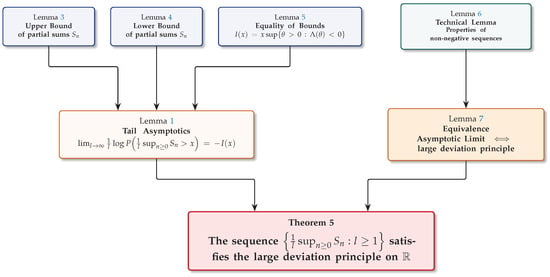
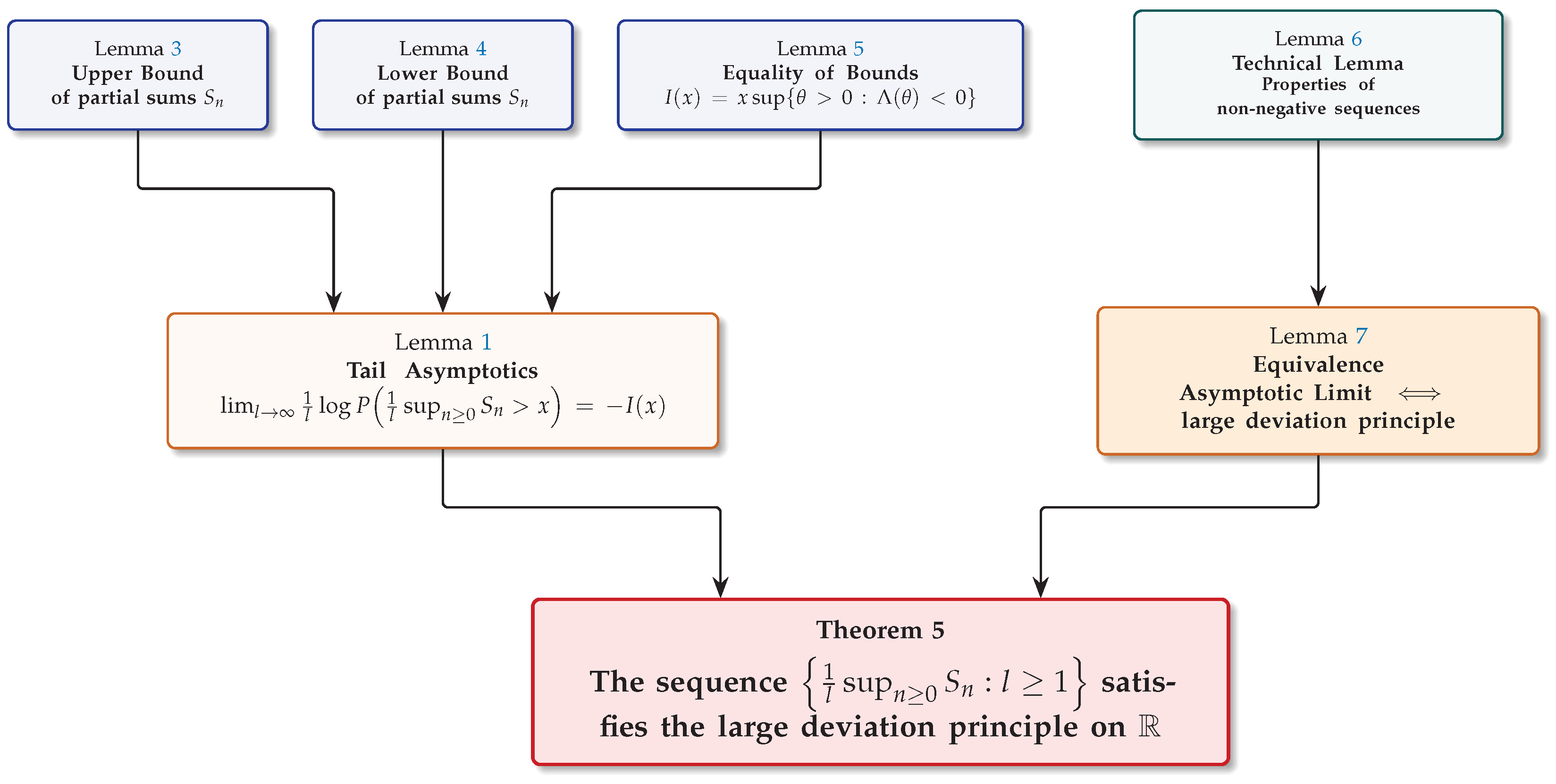
We synthesize the overall logical architecture for establishing Theorem 5 (our main result) in the following roadmap. This roadmap serves as a guide to navigate the key steps and lemma dependencies before delving into the detailed proof (Figure 1).

Figure 1. Logical roadmap of the proof for Theorem 5.

Explanation: The proof of Theorem 5 is structured as follows.

• Lemmas 3 and 4 provide the upper and lower bounds for the tail probability, respectively.
• Lemma 5 shows that these two bounds coincide, leading to the exact rate function $I\left(x\right)=xsup\{\theta >0:\mathsf{\Lambda }(\theta )<0\}$, which together form Lemma 1 (the asymptotic tail limit).
• Lemma 6 is a technical tool used to handle the difference between probabilities when establishing the lower bound.
• Lemma 7 establishes the equivalence between the asymptotic tail limit and the large deviation principle for non-negative random variables.
• The arrows indicate the logical relationship; the dashed line highlights the auxiliary role of Lemma 6.

Now, we present the detailed proof of Theorem 5.

First, by Lemma 1, under the conditions of Theorem 5, for all $x>0$,

$$\underset{l\to \infty }{lim}{\displaystyle \frac{1}{l}}logP\left({\displaystyle \frac{1}{l}}\underset{n\ge 0}{sup}{S}_n>x\right)=-I\left(x\right).$$

Second, since $S_0=0$, we have ${sup}_{n\ge 0}{S}_n\ge S_0=0$, i.e., $\left\{{\displaystyle \frac{1}{l}}{sup}_{n\ge 0}{S}_n:l\ge 1\right\}$ is a sequence of non-negative random variables, and since $I\left(x\right)=xsup\{\theta >0:\mathsf{\Lambda }(\theta )<0\}$, let ${\theta }^{*}=sup\{\theta >0:\mathsf{\Lambda }\left(\theta \right)<0\}$, then

• If ${\theta }^{*}=\infty$, then $I\left(x\right)=\left\{\begin{array}{cc}0,\hfill & x=0\hfill \\ \infty ,\hfill & x>0\hfill \end{array}\right.$;
• If ${\theta }^{*}<\infty$, then $I\left(x\right)={\theta }^{*}x$.

Clearly, $I\left(x\right)$ satisfies one of the two requirements in Lemma 7.

Therefore, by Lemma 7, for all $x>0$, ${lim}_{l\to \infty }{\displaystyle \frac{1}{l}}logP\left({\displaystyle \frac{1}{l}}{sup}_{n\ge 0}{S}_n>x\right)=-I\left(x\right)$ if and only if the large deviation principle holds, i.e.,

$$\underset{l\to \infty }{lim\; sup}{\displaystyle \frac{1}{l}}logP\left({\displaystyle \frac{1}{l}}\underset{n\ge 0}{sup}{S}_n\in F\right)\le -\underset{x\in F}{inf}I\left(x\right),\forall \mathrm{closed}\mathrm{set}F$$

$$\underset{l\to \infty }{lim\; inf}{\displaystyle \frac{1}{l}}logP\left({\displaystyle \frac{1}{l}}\underset{n\ge 0}{sup}{S}_n\in G\right)\ge -\underset{x\in G}{inf}I\left(x\right),\forall \mathrm{open}\mathrm{set}G$$

where $I\left(x\right)={inf}_{t\in {\mathbb{R}}^{+}}t{\mathsf{\Lambda }}^{*}\left({\displaystyle \frac{x}{t}}\right)=xsup\{\theta >0:\mathsf{\Lambda }\left(\theta \right)<0\}$. □

Proof of Corollary 1 .

Since $\{A_n:n\ge 1\}$ and $\{X_n:n\ge 1\}$ are independent, we obtain

$$\begin{array}{cc}\hfill {\mathsf{\Lambda }}_n^Y\left(\theta \right)& =logE\left[e^{\theta S_n^Y}\right]\hfill \\ & =logE\left[e^{\theta S_n^A}\right]+logE\left[e^{\theta S_n^X}\right]\hfill \\ & ={\mathsf{\Lambda }}_n^A\left(\theta \right)+{\mathsf{\Lambda }}_n^X\left(\theta \right),\hfill \end{array}$$

where ${\mathsf{\Lambda }}_n^A\left(\theta \right)=logE\left[e^{\theta S_n^A}\right]$, ${\mathsf{\Lambda }}_n^X\left(\theta \right)=logE\left[e^{\theta S_n^X}\right]$. And it is known that both ${\mathsf{\Lambda }}_A\left(\theta \right)$ and ${\mathsf{\Lambda }}_X\left(\theta \right)$ exist and are finite in a neighborhood of $\theta =0$. Then ${\mathsf{\Lambda }}_Y\left(\theta \right)={lim}_{n\to \infty }{\displaystyle \frac{1}{n}}{\mathsf{\Lambda }}_n^Y\left(\theta \right)={\mathsf{\Lambda }}_A\left(\theta \right)+{\mathsf{\Lambda }}_X\left(\theta \right)$ exists in $\mathbb{R}\cup \{\infty \}$ and is finite in a neighborhood of $\theta =0$. Since ${\mathsf{\Lambda }}_A\left(\theta \right)$ is differentiable in the interior of its effective domain, ${\mathsf{\Lambda }}_A\left(\theta \right)$ is continuous, and ${\mathsf{\Lambda }}_X\left(\theta \right)$ is lower semi-continuous, thus ${\mathsf{\Lambda }}_Y\left(\theta \right)$ is also lower semi-continuous. By the corollary condition, ${\mathsf{\Lambda }}_Y\left(\theta \right)$ is essentially smooth, and for each $n\ge 1$, when ${\mathsf{\Lambda }}_Y\left(\theta \right)<0$, ${\mathsf{\Lambda }}_n^Y\left(\theta \right)$ is finite.

Therefore, $\{Y_n:n\ge 1\}$ satisfies the conditions of the theorem, thus the corollary obviously holds. □

5. Proofs of Lemmas

To prove Lemma 1, we first provide the proofs of Lemmas 2–5:

Proof of Lemma 2 .

Since $E\left(X_1\right)=E\left(X_2\right)=\cdots =E\left(X_n\right)$, we have $E\left(S_n\right)=E(X_1+X_2+\cdots +X_n)=nE\left(X_1\right)$. Through the hypothesis of the theorem, we know $\mathsf{\Lambda }\left(\theta \right)$ is finite in a neighborhood of $\theta =0$, thus there exists $\delta >0$ such that for all $\theta \in (-\delta ,\delta )$, $\mathsf{\Lambda }\left(\theta \right)$ is finite. Because $\mathsf{\Lambda }\left(\theta \right)={lim}_{n\to \infty }{\displaystyle \frac{1}{n}}{\mathsf{\Lambda }}_n\left(\theta \right)$, the functions ${\mathsf{\Lambda }}_n\left(\theta \right)$ are also finite in $(-\delta ,\delta )$ of $\theta =0$ for all sufficiently large n. For each such n, Theorem 3 implies that ${\mathsf{\Lambda }}_n\left(\theta \right)$ is convex in $(-\delta ,\delta )$ and differentiable at $\theta =0$, with derivative ${\mathsf{\Lambda }}_n^{\prime }\left(0\right)=E\left(S_n\right)=nE\left(X_1\right)$.

Let $f_n\left(\theta \right)={\displaystyle \frac{1}{n}}{\mathsf{\Lambda }}_n\left(\theta \right)$. Since ${\mathsf{\Lambda }}_n\left(\theta \right)$ is convex, $f_n\left(\theta \right)$ is also convex in $(-\delta ,\delta )$, and $f_n\left(0\right)={\displaystyle \frac{1}{n}}{\mathsf{\Lambda }}_n\left(0\right)={\displaystyle \frac{1}{n}}logE\left[e^{0·S_n}\right]=0$, $f_n^{\prime }\left(0\right)={\displaystyle \frac{1}{n}}{\mathsf{\Lambda }}_n^{\prime }\left(0\right)=E\left(X_1\right)$.

By Theorem 2 the pointwise limit $\mathsf{\Lambda }$ is convex. The hypotheses that $\mathsf{\Lambda }\left(\theta \right)$ is finite near the origin and essentially smooth guarantee its differentiability at 0. Consequently, ${\mathsf{\Lambda }}^{\prime }\left(0\right)=E\left(X_1\right)$. □

Proof of Lemma 3 .

Since

$$\left\{\underset{n\ge 0}{sup}{S}_n>lx\right\}=\left\{\underset{n\ge 1}{sup}{S}_n>lx\right\}=\bigcup _{n=1}^{\infty }\left\{S_n>lx\right\}.$$

We easily obtain

$$\begin{array}{cc}\hfill P\left({\displaystyle \frac{{sup}_{n\ge 0}{S}_n}{l}}>x\right)& =P\left(\underset{n\ge 1}{sup}{S}_n>lx\right)\hfill \\ & =P\left(\bigcup _{n=1}^{\infty }\{S_n>lx\}\right)\hfill \\ & \le \sum _{n=1}^{\infty }P\left(S_n\ge lx\right)\hfill \\ & =\sum _{n=1}^{\infty }P\left(\theta S_n\ge \theta lx\right)(\forall \theta >0)\hfill \\ & =\sum _{n=1}^{\infty }P\left(e^{\theta S_n}\ge e^{\theta lx}\right)\hfill \\ & \le \sum _{n=1}^{\infty }{\displaystyle \frac{E\left(e^{\theta S_n}\right)}{e^{\theta lx}}}\hfill \\ & =e^{-\theta lx}\sum _{n=1}^{\infty }{e}^{{\mathsf{\Lambda }}_n\left(\theta \right)}.\hfill \end{array}$$

Now there exists $\theta >0$ such that $\mathsf{\Lambda }\left(\theta \right)<0$. Indeed, since $\mathsf{\Lambda }\left(\theta \right)={lim}_{n\to \infty }{\displaystyle \frac{1}{n}}{\mathsf{\Lambda }}_n\left(\theta \right)$ exists, and by Lemma 2 together with Theorem 2 we have ${\mathsf{\Lambda }}^{\prime }\left(0\right)=E\left(X_1\right)$, and based the assumption $E\left(X_1\right)<0$, we have ${\mathsf{\Lambda }}^{\prime }\left(0\right)<0$. Consequently, by the definition of the derivative, there is some $\theta >0$ for which ${\displaystyle \frac{\mathsf{\Lambda }\left(\theta \right)-\mathsf{\Lambda }\left(0\right)}{\theta -0}}<0$, and hence $\mathsf{\Lambda }\left(\theta \right)<0$. Choose $\epsilon >0$ such that $\mathsf{\Lambda }\left(\theta \right)<-2\epsilon \theta$. Since ${\displaystyle \frac{{\mathsf{\Lambda }}_n\left(\theta \right)}{n}}\to \mathsf{\Lambda }\left(\theta \right)$, there exists an integer $n_0$ such that for all $n>n_0$,

$$\left|{\displaystyle \frac{{\mathsf{\Lambda }}_n\left(\theta \right)}{n}}-\mathsf{\Lambda }\left(\theta \right)\right|<\epsilon \theta ,$$

i.e., ${\mathsf{\Lambda }}_n\left(\theta \right)<n(\mathsf{\Lambda }\left(\theta \right)+\epsilon \theta )<-n\epsilon \theta$.Therefore, we obtain the following.

$$\begin{array}{cc}\hfill e^{-\theta lx}\sum _{n=1}^{\infty }{e}^{{\mathsf{\Lambda }}_n\left(\theta \right)}& =e^{-\theta lx}\left(\sum _{n=1}^{n_0}{e}^{{\mathsf{\Lambda }}_n\left(\theta \right)}+\sum _{n=n_0+1}^{\infty }{e}^{{\mathsf{\Lambda }}_n\left(\theta \right)}\right)\hfill \\ & <e^{-\theta lx}\left(\sum _{n=1}^{n_0}{e}^{{\mathsf{\Lambda }}_n\left(\theta \right)}+\sum _{n=n_0+1}^{\infty }{e}^{-n\epsilon \theta }\right).\hfill \end{array}$$

On the one hand, based on the theorem’s assumption, when $\mathsf{\Lambda }\left(\theta \right)<0$, ${\mathsf{\Lambda }}_n\left(\theta \right)$ is finite for all n, thus there exists $K_1\left(n\right)>0$ such that ${\sum }_{n=1}^{n_0}{e}^{{\mathsf{\Lambda }}_n\left(\theta \right)}<K_1\left(n\right)<\infty$; on the other hand, ${\sum }_{n=n_0+1}^{\infty }{e}^{-n\epsilon \theta }$ is a geometric series with common ratio $e^{-\epsilon \theta }<1$, thus there exists $K_2\left(n\right)>0$ such that ${\sum }_{n=n_0+1}^{\infty }{e}^{-n\epsilon \theta }<K_2\left(n\right)<\infty$. Therefore, we have

$$\underset{l\to \infty }{lim\; sup}{\displaystyle \frac{1}{l}}logP\left({\displaystyle \frac{1}{l}}\underset{n\ge 0}{sup}{S}_n>x\right)\le -\theta x.$$

Taking the supremum over $\theta$, we get

$$\underset{l\to \infty }{lim\; sup}{\displaystyle \frac{1}{l}}logP\left({\displaystyle \frac{1}{l}}\underset{n\ge 0}{sup}{S}_n>x\right)\le -xsup\left\{\theta >0:\mathsf{\Lambda }\left(\theta \right)<0\right\}.$$

□

Proof of Lemma 4 .

For all $n\ge 0$,

$$P\left({\displaystyle \frac{1}{l}}\underset{n\ge 0}{sup}{S}_n>x\right)=P\left(\exists n:S_n>lx\right)\ge P\left(S_{\lceil lt\rceil }>lx\right).$$

where $\lceil x\rceil$ denotes the smallest integer not less than x (i.e., $\lceil x\rceil -1<x\le \lceil x\rceil$).

Therefore, we obtain the following.

$$\underset{l\to \infty }{lim\; inf}{\displaystyle \frac{1}{l}}logP\left({\displaystyle \frac{1}{l}}\underset{n\ge 0}{sup}{S}_n>x\right)\ge \underset{l\to \infty }{lim\; inf}{\displaystyle \frac{1}{l}}logP\left(S_{\lceil lt\rceil }>lx\right).$$

Since $l\le {\displaystyle \frac{\lceil lt\rceil }{t}}$, we have

$$\underset{l\to \infty }{lim\; inf}{\displaystyle \frac{1}{l}}logP\left({\displaystyle \frac{1}{l}}\underset{n\ge 0}{sup}{S}_n>x\right)\ge \underset{l\to \infty }{lim\; inf}{\displaystyle \frac{t}{\lceil lt\rceil }}logP\left(S_{\lceil lt\rceil }>{\displaystyle \frac{\lceil lt\rceil }{t}}·x\right).$$

Let $m=\lceil lt\rceil$, then, the following is the case.

$$\begin{array}{cc}\hfill \underset{l\to \infty }{lim\; inf}{\displaystyle \frac{1}{l}}logP\left({\displaystyle \frac{1}{l}}\underset{n\ge 0}{sup}{S}_n>x\right)& \ge t\underset{m\to \infty }{lim\; inf}{\displaystyle \frac{1}{m}}logP\left(S_m>{\displaystyle \frac{mx}{t}}\right)\hfill \\ & =t\underset{m\to \infty }{lim\; inf}{\displaystyle \frac{1}{m}}logP\left({\displaystyle \frac{S_m}{m}}>{\displaystyle \frac{x}{t}}\right).\hfill \end{array}$$

By the lower bound of the Gärtner–Ellis theorem, for the open set $G=\left({\displaystyle \frac{x}{t}},\infty \right)$, we have

$$\underset{m\to \infty }{lim\; inf}{\displaystyle \frac{1}{m}}logP\left({\displaystyle \frac{S_m}{m}}>{\displaystyle \frac{x}{t}}\right)\ge -\underset{y\in G}{inf}{\mathsf{\Lambda }}^{*}\left(y\right)\ge -{\mathsf{\Lambda }}^{*}\left({\left({\displaystyle \frac{x}{t}}\right)}^{+}\right).$$

Hence,

$$\underset{l\to \infty }{lim\; inf}{\displaystyle \frac{1}{l}}logP\left({\displaystyle \frac{1}{l}}\underset{n\ge 0}{sup}{S}_n>x\right)\ge -t{\mathsf{\Lambda }}^{*}\left({\left({\displaystyle \frac{x}{t}}\right)}^{+}\right).$$

Now we prove that ${\mathsf{\Lambda }}^{*}\left({\left({\displaystyle \frac{x}{t}}\right)}^{+}\right)={\mathsf{\Lambda }}^{*}\left({\displaystyle \frac{x}{t}}\right)$ for $x>0$ and $t>0$: By Theorem 4, ${\mathsf{\Lambda }}^{*}$ is increasing on $[E\left(X_1\right),\infty )$. For $x>0$ and $t>0$, we have ${\displaystyle \frac{x}{t}}>E\left(X_1\right)$ (since $E\left(X_1\right)<0$), thus ${\displaystyle \frac{x}{t}}$ lies in the interior of the effective domain of ${\mathsf{\Lambda }}^{*}$. Since a convex function is continuous in the interior of its effective domain, ${\mathsf{\Lambda }}^{*}$ is continuous at ${\displaystyle \frac{x}{t}}$, therefore ${\mathsf{\Lambda }}^{*}\left({\left({\displaystyle \frac{x}{t}}\right)}^{+}\right)={\mathsf{\Lambda }}^{*}\left({\displaystyle \frac{x}{t}}\right)$.

Taking the supremum over $t>0$, we get

$$\underset{l\to \infty }{lim\; inf}{\displaystyle \frac{1}{l}}logP\left({\displaystyle \frac{1}{l}}\underset{n\ge 0}{sup}{S}_n>x\right)\ge \underset{t>0}{sup}\left\{-t{\mathsf{\Lambda }}^{*}\left({\displaystyle \frac{x}{t}}\right)\right\}=-\underset{t>0}{inf}t{\mathsf{\Lambda }}^{*}\left({\displaystyle \frac{x}{t}}\right).$$

□

Proof of Lemma 5 

$$I\left(x\right)=\underset{t\in {\mathbb{R}}^{+}}{inf}t{\mathsf{\Lambda }}^{*}\left({\displaystyle \frac{x}{t}}\right)$$

$$=\underset{t\in {\mathbb{R}}^{+}}{inf}\underset{\theta \ge 0}{sup}\left\{\theta x-t\mathsf{\Lambda }\left(\theta \right)\right\}$$

$$=xsup\left\{\theta >0:\mathsf{\Lambda }\left(\theta \right)<0\right\}.$$

First, prove (1) = (2): Starting from expression (1), $I\left(x\right)={inf}_{t\in {\mathbb{R}}^{+}}t{\mathsf{\Lambda }}^{*}\left({\displaystyle \frac{x}{t}}\right)$. By the definition of ${\mathsf{\Lambda }}^{*}$ we obtain,

$${\mathsf{\Lambda }}^{*}\left({\displaystyle \frac{x}{t}}\right)=\underset{\theta \in \mathbb{R}}{sup}\left\{\theta ·{\displaystyle \frac{x}{t}}-\mathsf{\Lambda }\left(\theta \right)\right\}.$$

Therefore, we obtain the following.

$$t{\mathsf{\Lambda }}^{*}\left({\displaystyle \frac{x}{t}}\right)=t\underset{\theta \in \mathbb{R}}{sup}\left\{\theta ·{\displaystyle \frac{x}{t}}-\mathsf{\Lambda }\left(\theta \right)\right\}=\underset{\theta \in \mathbb{R}}{sup}\left\{\theta x-t\mathsf{\Lambda }\left(\theta \right)\right\}.$$

Then, taking the infimum over $t>0$ on both sides yields, we have

$$\underset{t\in {\mathbb{R}}^{+}}{inf}t{\mathsf{\Lambda }}^{*}\left({\displaystyle \frac{x}{t}}\right)=\underset{t\in {\mathbb{R}}^{+}}{inf}\underset{\theta \in \mathbb{R}}{sup}\left\{\theta x-t\mathsf{\Lambda }\left(\theta \right)\right\}.$$

It remains to show that ${sup}_{\theta \in \mathbb{R}}\left\{\theta x-t\mathsf{\Lambda }\left(\theta \right)\right\}={sup}_{\theta \ge 0}\left\{\theta x-t\mathsf{\Lambda }\left(\theta \right)\right\}$:

Since $\mathsf{\Lambda }\left(\theta \right)={lim}_{n\to \infty }{\displaystyle \frac{1}{n}}{\mathsf{\Lambda }}_n\left(\theta \right)$, i.e., $\mathsf{\Lambda }\left(\theta \right)$ is the limit of the convex function sequence ${\displaystyle \frac{1}{n}}{\mathsf{\Lambda }}_n\left(\theta \right)$, by Theorem 2, $\mathsf{\Lambda }\left(\theta \right)$ is convex, and by direct computation we get $\mathsf{\Lambda }\left(0\right)=0$. By Lemma 2, we have ${\mathsf{\Lambda }}^{\prime }\left(0\right)=E\left(X_1\right)<0$.

Let $g\left(\theta \right)=\theta x-t\mathsf{\Lambda }\left(\theta \right)$. Then:

1.

When $\theta =0$, we have $g\left(0\right)=0$;

2.

For $\theta <0$, by convexity $\mathsf{\Lambda }\left(\theta \right)\ge \mathsf{\Lambda }\left(0\right)+{\mathsf{\Lambda }}^{\prime }\left(0\right)\theta =\theta E\left(X_1\right)$, therefore

$$-t\mathsf{\Lambda }\left(\theta \right)\le -t\theta E\left(X_1\right).$$

Consequently,

$$g\left(\theta \right)=\theta x-t\mathsf{\Lambda }\left(\theta \right)\le \theta x-t\theta E\left(X_1\right)=\theta \left[x-tE\left(X_1\right)\right].$$

Since $x>0$, $t>0$, and $E\left(X_1\right)<0$, we get $x-tE\left(X_1\right)>0$, and $\theta <0$, thus $g\left(\theta \right)<0$.

Therefore, the following is the case:

$$\underset{\theta \in \mathbb{R}}{sup}\left\{\theta x-t\mathsf{\Lambda }\left(\theta \right)\right\}=\underset{\theta >0}{sup}\left\{\theta x-t\mathsf{\Lambda }\left(\theta \right)\right\}.$$

Next, prove (2) ≥ (3): For any $\theta >0$ satisfying $\mathsf{\Lambda }\left(\theta \right)<0$ and any $t\in {\mathbb{R}}^{+}$, we have

$$\underset{{\theta }^{\prime }\ge 0}{sup}\left\{{\theta }^{\prime }x-t\mathsf{\Lambda }\left({\theta }^{\prime }\right)\right\}\ge \theta x-t\mathsf{\Lambda }\left(\theta \right).$$

Since $\mathsf{\Lambda }\left(\theta \right)<0$, we have $\theta x-t\mathsf{\Lambda }\left(\theta \right)=\theta x+t(-\mathsf{\Lambda }(\theta \left)\right)\ge \theta x$, which holds for all $\theta >0$ such that $\mathsf{\Lambda }\left(\theta \right)<0$.

Thus, we obtain the following.

$$\underset{{\theta }^{\prime }\ge 0}{sup}\left\{{\theta }^{\prime }x-t\mathsf{\Lambda }\left({\theta }^{\prime }\right)\right\}\ge \theta x.$$

Taking the supremum over $\theta$, we can obtain

$$\underset{{\theta }^{\prime }\ge 0}{sup}\left\{{\theta }^{\prime }x-t\mathsf{\Lambda }\left({\theta }^{\prime }\right)\right\}\ge \underset{\begin{array}{c}\theta >0:\mathsf{\Lambda }\left(\theta \right)<0\end{array}}{sup}\theta x=xsup\left\{\theta >0:\mathsf{\Lambda }\left(\theta \right)<0\right\}.$$

Since the left-hand side does not depend on t, taking the infimum over t, we get

$$\underset{t\in {\mathbb{R}}^{+}}{inf}\underset{{\theta }^{\prime }\ge 0}{sup}\left\{{\theta }^{\prime }x-t\mathsf{\Lambda }\left({\theta }^{\prime }\right)\right\}\ge xsup\left\{\theta >0:\mathsf{\Lambda }\left(\theta \right)<0\right\}.$$

Thus, we complete the proof of (2)≥(3).

Finally, we prove (2) ≤ (3): Let ${\theta }^{*}=sup\left\{\theta >0:\mathsf{\Lambda }\left(\theta \right)<0\right\}$, and consider the following cases:

1.

If ${\theta }^{*}=\infty$, then for any $M>0$, there exists $\theta >M$ such that $\mathsf{\Lambda }\left(\theta \right)<0$. Then

$$\underset{\theta \ge 0}{sup}\left\{\theta x-t\mathsf{\Lambda }\left(\theta \right)\right\}\ge \theta x-t\mathsf{\Lambda }\left(\theta \right)\ge \theta x\ge Mx.$$

Since M is arbitrary, ${sup}_{\theta >0}\left\{\theta x-t\mathsf{\Lambda }\left(\theta \right)\right\}=\infty$, so (2) = ∞, and (3) = ∞, thus under condition 1, we have established (2) ≤ (3).

2.

If ${\theta }^{*}$ is in the interior of the effective domain of $\mathsf{\Lambda }$, its essential smoothness implies differentiability (and hence continuity) at ${\theta }^{*}$; therefore $\mathsf{\Lambda }\left({\theta }^{*}\right)=0$ and ${\mathsf{\Lambda }}^{\prime }\left({\theta }^{*}\right)>0$. Since $\mathsf{\Lambda }\left(\theta \right)$ is convex, for all $\theta \ge 0$, we have

$$\mathsf{\Lambda }\left(\theta \right)\ge \mathsf{\Lambda }\left({\theta }^{*}\right)+{\mathsf{\Lambda }}^{\prime }\left({\theta }^{*}\right)(\theta -{\theta }^{*})={\mathsf{\Lambda }}^{\prime }\left({\theta }^{*}\right)(\theta -{\theta }^{*}).$$

The following is the case:

$$\begin{array}{cc}\hfill \theta x-t\mathsf{\Lambda }\left(\theta \right)& \le \theta x-t{\mathsf{\Lambda }}^{\prime }\left({\theta }^{*}\right)(\theta -{\theta }^{*})\hfill \\ & =\theta x-t{\mathsf{\Lambda }}^{\prime }\left({\theta }^{*}\right)\theta +t{\mathsf{\Lambda }}^{\prime }\left({\theta }^{*}\right){\theta }^{*}\hfill \\ & =\theta \left[x-t{\mathsf{\Lambda }}^{\prime }\left({\theta }^{*}\right)\right]+t{\mathsf{\Lambda }}^{\prime }\left({\theta }^{*}\right){\theta }^{*}.\hfill \end{array}$$

Let $\alpha =x-t{\mathsf{\Lambda }}^{\prime }\left({\theta }^{*}\right)$, $\beta =t{\mathsf{\Lambda }}^{\prime }\left({\theta }^{*}\right){\theta }^{*}$, then

$$\begin{array}{cc}\hfill \underset{\theta \ge 0}{sup}\left\{\theta x-t\mathsf{\Lambda }\left(\theta \right)\right\}& \le \underset{\theta \ge 0}{sup}\left\{\theta \alpha +\beta \right\}\hfill \\ \hfill & =\left\{\begin{array}{cc}\beta ,\hfill & \mathrm{if}\alpha \le 0\hfill \\ \infty ,\hfill & \mathrm{if}\alpha >0\hfill \end{array}\right.\hfill \\ \hfill & =\left\{\begin{array}{cc}t{\theta }^{*}{\mathsf{\Lambda }}^{\prime }\left({\theta }^{*}\right),\hfill & \mathrm{if}t\ge {\displaystyle \frac{x}{{\mathsf{\Lambda }}^{\prime }\left({\theta }^{*}\right)}}\hfill \\ \infty ,\hfill & \mathrm{if}t<{\displaystyle \frac{x}{{\mathsf{\Lambda }}^{\prime }\left({\theta }^{*}\right)}}.\hfill \end{array}\right.\hfill \end{array}$$

Therefore, we obtain the following.

$$\begin{array}{cc}\hfill \underset{t\in {\mathbb{R}}^{+}}{inf}\underset{\theta \ge 0}{sup}\left\{\theta x-t\mathsf{\Lambda }\left(\theta \right)\right\}& \le \underset{\begin{array}{c}t\ge {\displaystyle \frac{x}{{\mathsf{\Lambda }}^{\prime }\left({\theta }^{*}\right)}}\end{array}}{inf}t{\theta }^{*}{\mathsf{\Lambda }}^{\prime }\left({\theta }^{*}\right)\hfill \\ & ={\theta }^{*}x\hfill \\ & =xsup\left\{\theta >0:\mathsf{\Lambda }\left(\theta \right)<0\right\}.\hfill \end{array}$$

Thus, under condition 2, we complete the proof of (2) ≤ (3).

3.

If ${\theta }^{*}$ is on the boundary of the effective domain of $\mathsf{\Lambda }$, take a sequence $\left\{{\theta }_n\right\}$ such that ${\theta }_n\in (0,{\theta }^{*})$ and ${\theta }_n\uparrow {\theta }^{*}$. By convexity of $\mathsf{\Lambda }\left(\theta \right)$, for any $\theta >0$, we obtain

$$\mathsf{\Lambda }\left(\theta \right)\ge \mathsf{\Lambda }\left({\theta }_n\right)+{\mathsf{\Lambda }}^{\prime }\left({\theta }_n\right)(\theta -{\theta }_n).$$

Applying this to (2):

$$\begin{array}{cc}\hfill \left(2\right)& =\underset{t\in {\mathbb{R}}^{+}}{inf}\underset{\theta \ge 0}{sup}\left\{\theta x-t\mathsf{\Lambda }\left(\theta \right)\right\}\hfill \\ & \le \underset{t\in {\mathbb{R}}^{+}}{inf}\underset{\theta \ge 0}{sup}\left\{\theta x-t\mathsf{\Lambda }\left({\theta }_n\right)-t{\mathsf{\Lambda }}^{\prime }\left({\theta }_n\right)(\theta -{\theta }_n)\right\}\hfill \\ & =\underset{t\in {\mathbb{R}}^{+}}{inf}\underset{\theta \ge 0}{sup}\left\{\theta \left(x-t{\mathsf{\Lambda }}^{\prime }\left({\theta }_n\right)\right)+t\left({\theta }_n{\mathsf{\Lambda }}^{\prime }\left({\theta }_n\right)-\mathsf{\Lambda }\left({\theta }_n\right)\right)\right\}\hfill \\ & \le \underset{\begin{array}{c}t\ge {\displaystyle \frac{x}{{\mathsf{\Lambda }}^{\prime }\left({\theta }_n\right)}}\end{array}}{inf}t\left({\theta }_n{\mathsf{\Lambda }}^{\prime }\left({\theta }_n\right)-\mathsf{\Lambda }\left({\theta }_n\right)\right)\hfill \\ & ={\displaystyle \frac{x}{{\mathsf{\Lambda }}^{\prime }\left({\theta }_n\right)}}\left({\theta }_n{\mathsf{\Lambda }}^{\prime }\left({\theta }_n\right)-\mathsf{\Lambda }\left({\theta }_n\right)\right)\hfill \\ & =x{\theta }_n·{\displaystyle \frac{{\mathsf{\Lambda }}^{\prime }\left({\theta }_n\right)-\mathsf{\Lambda }\left({\theta }_n\right)/{\theta }_n}{{\mathsf{\Lambda }}^{\prime }\left({\theta }_n\right)}}.\hfill \end{array}$$

As $n\to \infty$, ${\theta }_n\to {\theta }^{*}$. By convexity of $\mathsf{\Lambda }(·)$, we have $\mathsf{\Lambda }\left({\theta }_n\right)\ge \mathsf{\Lambda }\left(0\right)+{\mathsf{\Lambda }}^{\prime }\left(0\right)({\theta }_n-0)={\mathsf{\Lambda }}^{\prime }\left(0\right){\theta }_n$. By the steepness assumption, ${\mathsf{\Lambda }}^{\prime }\left({\theta }_n\right)\to \infty$.

Therefore, when n is sufficiently large, ${\mathsf{\Lambda }}^{\prime }\left({\theta }_n\right)>0$, we can obtain

$${\displaystyle \frac{{\mathsf{\Lambda }}^{\prime }\left({\theta }_n\right)-\mathsf{\Lambda }\left({\theta }_n\right)/{\theta }_n}{{\mathsf{\Lambda }}^{\prime }\left({\theta }_n\right)}}\le {\displaystyle \frac{{\mathsf{\Lambda }}^{\prime }\left({\theta }_n\right)-{\mathsf{\Lambda }}^{\prime }\left(0\right)}{{\mathsf{\Lambda }}^{\prime }\left({\theta }_n\right)}}.$$

Taking the limsup of both sides over n, we have

$$\begin{array}{cc}\hfill \underset{n\to \infty }{lim\; sup}{\displaystyle \frac{{\mathsf{\Lambda }}^{\prime }\left({\theta }_n\right)-\mathsf{\Lambda }\left({\theta }_n\right)/{\theta }_n}{{\mathsf{\Lambda }}^{\prime }\left({\theta }_n\right)}}& \le \underset{n\to \infty }{lim\; sup}{\displaystyle \frac{{\mathsf{\Lambda }}^{\prime }\left({\theta }_n\right)-{\mathsf{\Lambda }}^{\prime }\left(0\right)}{{\mathsf{\Lambda }}^{\prime }\left({\theta }_n\right)}}\hfill \\ & =\underset{n\to \infty }{lim\; sup}\left(1-{\displaystyle \frac{{\mathsf{\Lambda }}^{\prime }\left(0\right)}{{\mathsf{\Lambda }}^{\prime }\left({\theta }_n\right)}}\right)\hfill \\ & =1.\hfill \end{array}$$

Thus, as $n\to \infty$, we obtain ${inf}_{t\in {\mathbb{R}}^{+}}{sup}_{\theta \ge 0}\left\{\theta x-t\mathsf{\Lambda }\left(\theta \right)\right\}\le {\theta }^{*}x=xsup\left\{\theta >0:\mathsf{\Lambda }\left(\theta \right)<0\right\}$. We conclude that, under condition 3, the inequality (2)≤(3) is valid. This completes the proof of the lemma.

Combining the above three cases, we have proved (2) ≤ (3). Together with the previous result (2) ≥ (3), we obtain (2) = (3). Now we complete the proof of Lemma 5. □

Proof of Lemma 1 .

The large deviation upper bound is proved by Lemmas 2 and 3, the lower bound is proved by Lemma 4, and finally Lemma 5 shows that the upper and lower bounds are equal. Thus, this completes the proof of Lemma 1. □

Proof of Lemma 6 .

1.

When condition (1) holds: since ${lim\; inf}_{n\to \infty }{\displaystyle \frac{1}{c_n}}log{a}_n\ge -a$, for any $\epsilon >0$ with $\epsilon <{\displaystyle \frac{b-a}{2}}$ there exists $k_1$ such that for all $n\ge k_1$,

$${\displaystyle \frac{1}{c_n}}log{a}_n>\underset{n\to \infty }{lim\; inf}{\displaystyle \frac{1}{c_n}}log{a}_n-\epsilon \ge -a-\epsilon ,$$

i.e., $a_n>e^{-(a+\epsilon )c_n}$.

From ${lim\; sup}_{n\to \infty }{\displaystyle \frac{1}{c_n}}log{b}_n\le -b$, we take the same number $\epsilon$ as above, there exists $k_2$ such that when $n\ge k_2$,

$${\displaystyle \frac{1}{c_n}}log{b}_n<\underset{n\to \infty }{lim\; sup}{\displaystyle \frac{1}{c_n}}log{b}_n+\epsilon \le -b+\epsilon ,$$

i.e., $b_n<e^{-(b-\epsilon )c_n}$.

Let $k_0=max\{k_1,k_2\}$. Then for every $n\ge k_0$, combining the above two inequalities we have

$$a_n-b_n>e^{-(a+\epsilon )c_n}-e^{-(b-\epsilon )c_n}=e^{-(a+\epsilon )c_n}\left(1-e^{-(b-a-2\epsilon )c_n}\right).$$

Taking the liminf of the logarithm as $n\to \infty$ on both sides, the following is obtained.

$$\underset{n\to \infty }{lim\; inf}{\displaystyle \frac{1}{c_n}}log(a_n-b_n)\ge -(a+\epsilon ).$$

Then, letting $\epsilon \downarrow 0$ we obtain

$${\displaystyle \underset{n\to \infty }{lim\; inf}\frac{1}{c_n}log(a_n-b_n)\ge -a.}$$

2.

When condition (2) holds: since ${lim\; inf}_{n\to \infty }{\displaystyle \frac{1}{c_n}}log{a}_n\ge -a$, for any $\epsilon >0$ there exists $k_1$ such that for all $n\ge k_1$,

$${\displaystyle \frac{1}{c_n}}log{a}_n>\underset{n\to \infty }{lim\; inf}{\displaystyle \frac{1}{c_n}}log{a}_n-\epsilon \ge -a-\epsilon ,$$

i.e., $a_n>e^{-(a+\epsilon )c_n}$.

From ${lim\; sup}_{n\to \infty }{\displaystyle \frac{1}{c_n}}log{b}_n=-\infty$, for any $M>0$ satisfying $M>a+\epsilon$ there exists $k_2$ such that for all $n\ge k_2$,

$${\displaystyle \frac{1}{c_n}}log{b}_n<-M,$$

i.e., $b_n<e^{-M{c}_n}$.

Let $N=max\{k_1,k_2\}$. Then for every $n\ge N$, we have

$$a_n-b_n>e^{-(a+\epsilon )c_n}-e^{-M{c}_n}=e^{-(a+\epsilon )c_n}\left(1-e^{-(M-a-\epsilon )c_n}\right).$$

Taking the liminf of the logarithm as $n\to \infty$ on both sides, here, we obtain the following.

$$\underset{n\to \infty }{lim\; inf}{\displaystyle \frac{1}{c_n}}log(a_n-b_n)\ge -(a+\epsilon ).$$

Then, letting $\epsilon \downarrow 0$, we get

$$\underset{n\to \infty }{lim\; inf}{\displaystyle \frac{1}{c_n}}log(a_n-b_n)\ge -a.$$

Thus, we complete the proof of Lemma 6.

□

Proof of Lemma 7 .

1.

When condition (1) holds, i.e., $I\left(0\right)=0$ and for all $x>0$, $I\left(x\right)=\infty$.

(⇒) Since $\{X_n:n\ge 1\}$ satisfies the large deviation principle with speed $c_n$ and rate function $I\left(x\right)$, then for any $x>0$ we proceed as follows.

(1) Take the closed set $F=[x,\infty )$. Then ${inf}_{t\in [x,\infty )}I\left(t\right)=\infty$, and by the large deviation upper bound, we get

$$\underset{n\to \infty }{lim\; sup}{\displaystyle \frac{1}{c_n}}logP(X_n\in F)\le -\underset{t\in F}{inf}I\left(t\right)=-\infty .$$

Thus,

$$\underset{n\to \infty }{lim\; sup}{\displaystyle \frac{1}{c_n}}logP(X_n\ge x)\le -\infty .$$

Since $P(X_n>x)\le P(X_n\ge x)$, we obtain

$$\underset{n\to \infty }{lim\; sup}{\displaystyle \frac{1}{c_n}}logP(X_n>x)\le -\infty .$$

(2) Take the open set $G=(x,\infty )$. Then ${inf}_{t\in (x,\infty )}I\left(t\right)=\infty$, and by the large deviation lower bound, we obtain

$$\underset{n\to \infty }{lim\; inf}{\displaystyle \frac{1}{c_n}}logP(X_n\in G)\ge -\underset{x\in G}{inf}I\left(x\right)=-\infty .$$

Thus,

$$\underset{n\to \infty }{lim\; inf}{\displaystyle \frac{1}{c_n}}logP(X_n>x)\ge -\infty .$$

Combining the above two inequalities, we get

$$-\infty \le \underset{n\to \infty }{lim\; inf}{\displaystyle \frac{1}{c_n}}logP(X_n>x)\le \underset{n\to \infty }{lim\; sup}{\displaystyle \frac{1}{c_n}}logP(X_n>x)\le -\infty ,$$

which is equivalent to

$$\underset{n\to \infty }{lim}{\displaystyle \frac{1}{c_n}}logP(X_n>x)=-\infty =-I\left(x\right).$$

(⇐) For any closed set $F\subset \mathbb{R}$: Let $a=minF$, then $a\ge 0$ and $F\subset [a,\infty )$, we have

$$P(X_n\in F)\le P(X_n\ge a).$$

(1) If $a>0$, for any $m\ge 1$ with $a-{\displaystyle \frac{1}{m}}>0$, we have $P(X_n\ge a)\le P\left(X_n>a-{\displaystyle \frac{1}{m}}\right)$. Thus,

$$\begin{array}{cc}\hfill \underset{n\to \infty }{lim\; sup}{\displaystyle \frac{1}{c_n}}logP(X_n\ge a)& \le \underset{n\to \infty }{lim\; sup}{\displaystyle \frac{1}{c_n}}logP\left(X_n>a-{\displaystyle \frac{1}{m}}\right)\hfill \\ & =-I\left(a-{\displaystyle \frac{1}{m}}\right)\hfill \\ & =-\infty .\hfill \end{array}$$

that is,

$$\underset{n\to \infty }{lim\; sup}{\displaystyle \frac{1}{c_n}}logP(X_n\ge a)=-\infty .$$

Then, the following is the case:

$$\underset{n\to \infty }{lim\; sup}{\displaystyle \frac{1}{c_n}}logP(X_n\in F)\le \underset{n\to \infty }{lim\; sup}{\displaystyle \frac{1}{c_n}}logP(X_n\ge a)=-\infty =-\underset{x\in F}{inf}I\left(x\right).$$

(2) If $a=0$, then $0\in F$ and $F\subset [0,\infty )$. Since $0\in F$, we have ${inf}_{x\in F}I\left(x\right)\le I\left(0\right)=0$, moreover, because $I\left(x\right)\ge 0$ for any $x>0$, we get ${inf}_{x\in F}I\left(x\right)=0$. Also, since $P(X_n\in F)\le 1$, we have ${\displaystyle \frac{1}{c_n}}logP(X_n\in F)\le 0$. Thus,

$$\underset{n\to \infty }{lim\; sup}{\displaystyle \frac{1}{c_n}}logP(X_n\in F)\le 0=-\underset{x\in F}{inf}I\left(x\right).$$

For any open set $G\subset \mathbb{R}$:

(1) If $0\notin G$, then $G\subset (0,\infty )$, so ${inf}_{x\in G}I\left(x\right)=\infty$, and obviously

$$\underset{n\to \infty }{lim\; inf}{\displaystyle \frac{1}{c_n}}logP(X_n\in G)\ge -\infty =-\underset{x\in G}{inf}I\left(x\right).$$

(2) If $0\in G$, since G is open, there exists $\delta >0$ such that $[0,\delta )\subset G$. Therefore,

$$P(X_n\in G)\ge P(0\le X_n<\delta )=1-P(X_n\ge \delta ).$$

Then, the following is the case:

$$\begin{array}{cc}\hfill \underset{n\to \infty }{lim\; inf}{\displaystyle \frac{1}{c_n}}logP(X_n\in G)& \ge \underset{n\to \infty }{lim\; inf}{\displaystyle \frac{1}{c_n}}logP(0\le X_n<\delta )\hfill \\ & =\underset{n\to \infty }{lim\; inf}{\displaystyle \frac{1}{c_n}}log\left[1-P(X_n\ge \delta )\right].\hfill \end{array}$$

We now prove that ${lim\; sup}_{n\to \infty }{\displaystyle \frac{1}{c_n}}logP(X_n\ge \delta )=-\infty$: For any $m\ge 1$ with $\delta -{\displaystyle \frac{1}{m}}>0$, we have $P(X_n\ge \delta )\le P\left(X_n>\delta -{\displaystyle \frac{1}{m}}\right)$, consequently,

$$\underset{n\to \infty }{lim\; sup}{\displaystyle \frac{1}{c_n}}logP\left(X_n>\delta -{\displaystyle \frac{1}{m}}\right)=-I\left(\delta -{\displaystyle \frac{1}{m}}\right)=-\infty .$$

Thus,

$$\underset{n\to \infty }{lim\; sup}{\displaystyle \frac{1}{c_n}}logP(X_n\ge \delta )=-\infty .$$

By Lemma 6, we have

$$\underset{n\to \infty }{lim\; inf}{\displaystyle \frac{1}{c_n}}log\left(1-P(X_n\ge \delta )\right)\ge 0.$$

Since $0\in G$ and $I\left(0\right)=0$, we have ${inf}_{x\in G}I\left(x\right)=0$. Therefore, we obtain the following.

$$\underset{n\to \infty }{lim\; inf}{\displaystyle \frac{1}{c_n}}logP(X_n\in G)\ge 0=-\underset{x\in G}{inf}I\left(x\right).$$

2.

When condition (2) holds, i.e., $I\left(0\right)=0$, and for all $x>0$ we have $I\left(x\right)<\infty$, and $I\left(x\right)$ is strictly increasing, lower semi-continuous, and right-continuous.

(⇒) Since $\{X_n:n\ge 1\}$ satisfies the large deviation principle with speed $c_n$ and the rate function $I\left(x\right)$, then for any $x>0$:

(1) Take the open set $G=(x,\infty )$. By the large deviation lower bound,

$$\underset{n\to \infty }{lim\; inf}{\displaystyle \frac{1}{c_n}}logP(X_n>x)\ge -\underset{t\in (x,\infty )}{inf}I\left(t\right).$$

Since I is strictly increasing, ${inf}_{t\in (x,\infty )}I\left(t\right)=I\left(x^{+}\right)$, and because I is right-continuous, $I\left(x^{+}\right)=I\left(x\right)$. Thus,

$$\underset{n\to \infty }{lim\; inf}{\displaystyle \frac{1}{c_n}}logP(X_n>x)\ge -I\left(x\right).$$

(2) Take the closed set $F=[x,\infty )$. By the large deviation upper bound,

$$\underset{n\to \infty }{lim\; sup}{\displaystyle \frac{1}{c_n}}logP(X_n\ge x)\le -\underset{t\in [x,\infty )}{inf}I\left(t\right)=-I\left(x\right).$$

Since $P(X_n>x)\le P(X_n\ge x)$, we have

$$\underset{n\to \infty }{lim\; sup}{\displaystyle \frac{1}{c_n}}logP(X_n>x)\le -I\left(x\right).$$

Combining the above two inequalities, we get

$$-I\left(x\right)\le \underset{n\to \infty }{lim\; inf}{\displaystyle \frac{1}{c_n}}logP(X_n>x)\le \underset{n\to \infty }{lim\; sup}{\displaystyle \frac{1}{c_n}}logP(X_n>x)\le -I\left(x\right),$$

which is equivalent to

$$\underset{n\to \infty }{lim}{\displaystyle \frac{1}{c_n}}logP(X_n>x)=-I\left(x\right).$$

(⇐) For any closed set F: Let $a=minF$, then $a\ge 0$ and $F\subset [a,\infty )$, thus

$$P(X_n\in F)\le P(X_n\ge a).$$

For any $0<\epsilon <a$, we have $P(X_n\ge a)\le P(X_n>a-\epsilon )$. Based on the assumption,

$$\underset{n\to \infty }{lim\; sup}{\displaystyle \frac{1}{c_n}}logP(X_n>a-\epsilon )=\underset{n\to \infty }{lim}{\displaystyle \frac{1}{c_n}}logP(X_n>a-\epsilon )=-I(a-\epsilon ).$$

Since I is lower semi-continuous, then letting $\epsilon \downarrow 0$ we obtain

$$\underset{n\to \infty }{lim\; sup}{\displaystyle \frac{1}{c_n}}logP(X_n\in F)\le -I\left(a\right)=-\underset{x\in F}{inf}I\left(x\right).$$

For any open set G:

(1) If $0\notin G$, since G is open, for any $x\in G$, there exists $\delta >0$ such that $(x-\delta ,x+\delta )\subset G$. Then

$$\begin{array}{cc}\hfill P(X_n\in G)& \ge P\left(X_n\in (x-\delta ,x+\delta )\right)\hfill \\ & =P(X_n>x-\delta )-P(X_n\ge x+\delta ).\hfill \end{array}$$

For any ${\eta }_1>0$ with $x+\delta -{\eta }_1>0$, we have

$$P(X_n\ge x+\delta )\le P(X_n>x+\delta -{\eta }_1).$$

$$P(X_n>x-\delta )\ge P(X_n>x-\delta +{\eta }_1).$$

By the hypothesis, we get

$$\underset{n\to \infty }{lim}{\displaystyle \frac{1}{c_n}}logP(X_n>x-\delta )=-I(x-\delta ),$$

$$\underset{n\to \infty }{lim}{\displaystyle \frac{1}{c_n}}logP(X_n>x+\delta )=-I(x+\delta ).$$

Then,

$$\begin{array}{cc}\hfill \underset{n\to \infty }{lim\; sup}{\displaystyle \frac{1}{c_n}}logP(X_n\ge x+\delta )& =\underset{n\to \infty }{lim}{\displaystyle \frac{1}{c_n}}logP(X_n\ge x+\delta )\hfill \\ & \le \underset{n\to \infty }{lim}{\displaystyle \frac{1}{c_n}}logP(X_n>x+\delta -{\eta }_1)\hfill \\ & =-I(x+\delta -{\eta }_1).\hfill \end{array}$$

$$\begin{array}{cc}\hfill \underset{n\to \infty }{lim\; inf}{\displaystyle \frac{1}{c_n}}logP(X_n>x-\delta )& =\underset{n\to \infty }{lim}{\displaystyle \frac{1}{c_n}}logP(X_n>x-\delta )\hfill \\ & \ge \underset{n\to \infty }{lim}{\displaystyle \frac{1}{c_n}}logP(X_n>x-\delta +{\eta }_1)\hfill \\ & =-I(x-\delta +{\eta }_1).\hfill \end{array}$$

Moreover, since I is lower semi-continuous, then letting ${\eta }_1\downarrow 0$ we have

$$\underset{n\to \infty }{lim\; sup}{\displaystyle \frac{1}{c_n}}logP(X_n\ge x+\delta )\le -I(x+\delta ).$$

$$\underset{n\to \infty }{lim\; inf}{\displaystyle \frac{1}{c_n}}logP(X_n>x-\delta )\ge -I(x-\delta ).$$

Since $I\left(x\right)$ is strictly increasing, we have $I(x-\delta )<I\left(x\right)<I(x+\delta )$. Let $a_n=P(X_n>x-\delta )$, $b_n=P(X_n\ge x+\delta )$, $a=I(x-\delta )$, $b=I(x+\delta )$. Then, by Lemma 6, we can obtain

$$\underset{n\to \infty }{lim\; inf}{\displaystyle \frac{1}{c_n}}logP(X_n\in (x-\delta ,x+\delta ))\ge -I(x-\delta ).$$

Thus, the following is the case:

$$\begin{array}{cc}\hfill \underset{n\to \infty }{lim\; inf}{\displaystyle \frac{1}{c_n}}logP(X_n\in G)& \ge \underset{n\to \infty }{lim\; inf}{\displaystyle \frac{1}{c_n}}logP(X_n\in (x-\delta ,x+\delta ))\hfill \\ & \ge -I\left(x\right).\hfill \end{array}$$

Taking the supremum over all $x\in G$, we get

$$\underset{n\to \infty }{lim\; inf}{\displaystyle \frac{1}{c_n}}logP(X_n\in G)\ge -\underset{x\in G}{inf}I\left(x\right).$$

(2) If $0\in G$, since G is open, there exists $\delta >0$ such that $[0,\delta )\subset G$. Therefore,

$$\begin{array}{cc}\hfill P(X_n\in G)& \ge P(0\le X_n<\delta )\hfill \\ & =1-P(X_n\ge \delta ).\hfill \end{array}$$

For any ${\eta }_2>0$ with $\delta -{\eta }_2>0$, we have

$$P(X_n\ge \delta )\le P(X_n>\delta -{\eta }_2).$$

By the hypothesis, we can obtain

$$\underset{n\to \infty }{lim}{\displaystyle \frac{1}{c_n}}logP(X_n>\delta )=-I\left(\delta \right).$$

Thus, the following is the case:

$$\begin{array}{cc}\hfill \underset{n\to \infty }{lim\; sup}{\displaystyle \frac{1}{c_n}}logP(X_n\ge \delta )& \le \underset{n\to \infty }{lim\; sup}{\displaystyle \frac{1}{c_n}}logP(X_n>\delta -{\eta }_2)\hfill \\ & =\underset{n\to \infty }{lim}{\displaystyle \frac{1}{c_n}}logP(X_n>\delta -{\eta }_2)\hfill \\ & =-I(\delta -{\eta }_2).\hfill \end{array}$$

Since $I(·)$ is lower semi-continuous, letting ${\eta }_2\downarrow 0$, we obtain the following.

$$\underset{n\to \infty }{lim\; sup}{\displaystyle \frac{1}{c_n}}logP(X_n\ge \delta )\le -I\left(\delta \right).$$

Because $I(·)$ is strictly increasing and $I\left(0\right)=0$, we have $I\left(\delta \right)>0$. Then, the following is the case.

$$\begin{array}{cc}\hfill \underset{n\to \infty }{lim\; inf}{\displaystyle \frac{1}{c_n}}logP(X_n\in G)& \ge \underset{n\to \infty }{lim\; inf}{\displaystyle \frac{1}{c_n}}logP(0\le X_n<\delta )\hfill \\ & =\underset{n\to \infty }{lim\; inf}{\displaystyle \frac{1}{c_n}}log\left[P(X_n\ge 0)-P(X_n\ge \delta )\right]\hfill \\ & =\underset{n\to \infty }{lim\; inf}{\displaystyle \frac{1}{c_n}}log\left[1-P(X_n\ge \delta )\right].\hfill \end{array}$$

Since ${lim\; inf}_{n\to \infty }{\displaystyle \frac{1}{c_n}}log1=0$, and

$$\begin{array}{cc}\hfill \underset{n\to \infty }{lim\; sup}{\displaystyle \frac{1}{c_n}}logP(X_n\ge \delta )& \ge \underset{n\to \infty }{lim\; sup}{\displaystyle \frac{1}{c_n}}logP(X_n>\delta )\hfill \\ & =\underset{n\to \infty }{lim}{\displaystyle \frac{1}{c_n}}logP(X_n>\delta )\hfill \\ & =-I\left(\delta \right).\hfill \end{array}$$

By Lemma 6, we have

$$\underset{n\to \infty }{lim\; inf}{\displaystyle \frac{1}{c_n}}logP(X_n\in G)\ge 0=-\underset{x\in G}{inf}I\left(x\right).$$

Thus, we complete the proof of Lemma 7.

□

6. Application Examples

Theorem 5 states that, under the assumptions given in Section 3, the sequence $\left\{{\displaystyle \frac{1}{l}}{sup}_{n\ge 0}{S}_n:l\ge 1\right\}$ satisfies a large deviation principle, with rate function

$$I\left(x\right)=\underset{t>0}{inf}t{\mathsf{\Lambda }}^{*}\left({\displaystyle \frac{x}{t}}\right)=xsup\{\theta >0:\mathsf{\Lambda }\left(\theta \right)<0\}.$$

Equivalently, for any $x>0$, we have

$$\underset{l\to \infty }{lim}{\displaystyle \frac{1}{l}}logP\left(\left\{{\displaystyle \frac{1}{l}}\underset{n\ge 0}{sup}{S}_n>x\right\}\right)=-I\left(x\right).$$

This means that, when the threshold increases with the scale parameter, the probability of the event $\left\{{\displaystyle \frac{1}{l}}{sup}_{n\ge 0}{S}_n>x\right\}$ decays exponentially, and the decay rate is precisely characterized by $I\left(x\right)$.

This is exactly the type of problem addressed in the application scenarios of Section 6. In queueing systems, communication networks, and edge computing, ${sup}_{k\ge 0}{S}_k$ can represent the peak of cumulative input (or workload); therefore, the event $\left\{{sup}_{k\ge 0}{S}_k>lx\right\}$ can correspond to rare but high-impact risk situations such as queue buildup, buffer stress, and delay spikes. The rate function provided by Theorem 5 can therefore be used to quantitatively evaluate the probability-decay behavior of such extreme-risk events.

We now present two application examples to illustrate the practical use of the above theoretical results.

Example 1.

First-Order Autoregressive Process Model

In queuing theory and communication networks, understanding the extreme behavior of stochastic processes is essential for characterizing system performance. This section demonstrates the application of the aforementioned large deviation theorem through an example of a first-order autoregressive process.

Consider a first-order autoregressive process with negative drift: $A_n=X_n+\mu$, $\mu <0$, where $A_n$ represents the workload arriving at the queue at time n, and $X_n=\alpha X_{n-1}+{\epsilon }_n$, with $\left|\alpha \right|<1$, and $\{{\epsilon }_n:n\ge 1\}$ is a sequence of independent and identically distributed standard normal random variables. We take the initial state $X_0\sim N\left(0,{\displaystyle \frac{1}{1-{\alpha }^2}}\right)$. Define the partial sums $S_n={\sum }_{k=1}^n{A}_k$ with $S_0=0$. We shall study the large deviation principle for $\left\{{\displaystyle \frac{1}{n}}{sup}_{k\ge 0}{S}_k:n\ge 1\right\}$.

By the stationarity of the AR(1) process, we have $E\left(X_n\right)=0$ for all $n\ge 1$. Therefore, $E\left(A_n\right)=E\left(X_n\right)+\mu =\mu <0$, then $E\left(A_1\right)=E\left(A_2\right)=\cdots =E\left(A_n\right)=\mu <0$.

Since both $\{X_n:n\ge 1\}$ and $\{A_n:n\ge 1\}$ are normal processes, it follows that $S_n$ obeys the normal distribution and has logarithmic moment generating function:

$$\begin{array}{cc}\hfill {\mathsf{\Lambda }}_n\left(\theta \right)& =logE\left[e^{\theta S_n}\right]\hfill \\ & =\theta E\left(S_n\right)+{\displaystyle \frac{1}{2}}{\theta }^{2}Var\left(S_n\right)\hfill \\ & =\theta n\mu +{\displaystyle \frac{1}{2}}{\theta }^{2}Var\left(S_n\right).\hfill \end{array}$$

The covariance function of the AR(1) process is $\gamma \left(k\right)=\mathrm{Cov}(X_n,X_{n+k})={\displaystyle \frac{{\alpha }^{\left|k\right|}}{1-{\alpha }^2}}$, $k=0,1,2,\cdots$, thus $\mathrm{Cov}(A_t,A_s)=\mathrm{Cov}(X_t,X_s)=\gamma \left(\right|t-s\left|\right)$.

Thus, we obtain the following.

$$\begin{array}{cc}\hfill Var\left(S_n\right)& =\sum _{i=1}^n\sum _{j=1}^n\mathrm{Cov}(A_i,A_j)\hfill \\ & =\sum _{i=1}^n\sum _{j=1}^n\gamma \left(\right|i-j\left|\right)\hfill \\ & =n\gamma \left(0\right)+2\sum _{k=1}^{n-1}(n-k)\gamma \left(k\right).\hfill \end{array}$$

Substituting $\gamma \left(0\right)={\displaystyle \frac{1}{1-{\alpha }^2}}$ and $\gamma \left(k\right)={\displaystyle \frac{{\alpha }^k}{1-{\alpha }^2}}$, and the following is the case:

$$\begin{array}{cc}\hfill Var\left(S_n\right)& ={\displaystyle \frac{n}{1-{\alpha }^2}}+{\displaystyle \frac{2}{1-{\alpha }^2}}\sum _{k=1}^{n-1}(n-k){\alpha }^k\hfill \\ & ={\displaystyle \frac{n}{1-{\alpha }^2}}+{\displaystyle \frac{2}{1-{\alpha }^2}}\left(\sum _{k=1}^{n-1}n{\alpha }^k-\sum _{k=1}^{n-1}k{\alpha }^k\right)\hfill \\ & ={\displaystyle \frac{n}{1-{\alpha }^2}}+{\displaystyle \frac{2}{1-{\alpha }^2}}\left[{\displaystyle \frac{n\alpha (1-{\alpha }^{n-1})}{1-\alpha }}-{\displaystyle \frac{\alpha (1-n{\alpha }^{n-1}+(n-1){\alpha }^n)}{{(1-\alpha )}^2}}\right].\hfill \end{array}$$

Because $\left|\alpha \right|<1$, we have ${\alpha }^n\to 0$ as $n\to \infty$, and consequently

$$\underset{n\to \infty }{lim}{\displaystyle \frac{1}{n}}Var\left(S_n\right)={\displaystyle \frac{1}{{(1-\alpha )}^2}}.$$

Thus, we obtain the following.

$$\begin{array}{cc}\hfill \mathsf{\Lambda }\left(\theta \right)& =\underset{n\to \infty }{lim}{\displaystyle \frac{1}{n}}{\mathsf{\Lambda }}_n\left(\theta \right)\hfill \\ & =\underset{n\to \infty }{lim}\left[\theta {\displaystyle \frac{E\left(S_n\right)}{n}}+{\displaystyle \frac{1}{2}}{\theta }^2{\displaystyle \frac{Var\left(S_n\right)}{n}}\right]\hfill \\ & =\theta \mu +{\displaystyle \frac{1}{2}}{\theta }^2·{\displaystyle \frac{1}{{(1-\alpha )}^2}}.\hfill \end{array}$$

Now, let ${\sigma }^2={\displaystyle \frac{1}{{(1-\alpha )}^2}}$, then we have $\mathsf{\Lambda }\left(\theta \right)=\theta \mu +{\displaystyle \frac{1}{2}}{\theta }^2{\sigma }^2$.

The sequence $\{A_n:n\ge 1\}$ satisfies all conditions of Theorem 5, and its rate function is given by:

$$\begin{array}{cc}\hfill I\left(x\right)& =xsup\{\theta >0:\mathsf{\Lambda }(\theta )<0\}\hfill \\ & =xsup\left\{\theta >0:\theta \mu +{\displaystyle \frac{1}{2}}{\theta }^2{\sigma }^2<0\right\}\hfill \\ & =x·\left(-{\displaystyle \frac{2\mu }{{\sigma }^2}}\right)\hfill \\ & =-2\mu {(1-\alpha )}^{2}x(\mathrm{for}\mathrm{all}x>0).\hfill \end{array}$$

By Theorem 5, $\left\{{\displaystyle \frac{1}{n}}{sup}_{k\ge 0}{S}_k:n\ge 1\right\}$ satisfies the large deviation principle. In particular, for all $x>0$:

$$\begin{array}{cc}\hfill \underset{n\to \infty }{lim}{\displaystyle \frac{1}{n}}logP\left({\displaystyle \frac{1}{n}}\underset{k\ge 0}{sup}{S}_k>x\right)& =-I\left(x\right)\hfill \\ & =2\mu {(1-\alpha )}^{2}x.\hfill \end{array}$$

Equivalently, for large n, we obtain the following.

$$P\left(\underset{k\ge 0}{sup}{S}_k>nx\right)\approx exp\left[2\mu {(1-\alpha )}^{2}nx\right].$$

Example 2.

First-Order Autoregressive Process and Poisson–Gaussian Mixture Model

In edge computing environments, the net task input received by each edge node over discrete time slots can be modeled as a Poisson–Gaussian autoregressive hybrid process. In particular, the Poisson component characterizes the baseline task arrivals induced by random user offloading and service request generation, whereas the Gaussian AR(1) component captures persistent correlated perturbations arising from service hotspots, spatiotemporal load fluctuations, variations in wireless channel conditions, and congestion propagation from upstream nodes. Even when the system satisfies the average negative drift condition—namely, that the long-run average service capacity of an edge node exceeds its average arrival load—the supremum of the cumulative net input may still be substantially amplified under short-term correlated shocks, thereby leading to queue accumulation, delay instability, and cascading local congestion.

Motivated by this application, let the net task input at time slot n be modeled as $Y_n=A_n+K_n$, where $\{A_n:n\ge 1\}$ is a sequence of independent and identically distributed Poisson random variables with parameter λ, and $K_n=X_n+\mu$, with $\{X_n:n\ge 1\}$ being a stationary first-order autoregressive (AR(1)) process defined by

$$X_n=\alpha X_{n-1}+\sqrt{1-{\alpha }^2}{\epsilon }_n,\left|\alpha \right|<1,$$

where $\{{\epsilon }_n:n\ge 1\}$ is an i.i.d. sequence of standard normal random variables. The two sequences $\left\{A_n\right\}$ and $\left\{K_n\right\}$ are assumed to be independent. Define the partial sums $S_n^Y={\sum }_{k=1}^n{Y}_k$ and let $Q={sup}_{n\ge 0}{S}_n^Y$. We assume $E\left[Y_n\right]=\lambda +\mu <0$ (i.e., $\mu <-\lambda$) and study the large deviation principle for $\left\{{\displaystyle \frac{Q}{n}}:n\ge 1\right\}$.

Since $Y_n=A_n+K_n$ and $A_n$ and $K_n$ are independent, we have $E\left[e^{\theta S_n^Y}\right]=E\left[e^{\theta {\sum }_{i=1}^n{A}_i}\right]·E\left[e^{\theta {\sum }_{i=1}^n{K}_i}\right]$, where $S_n^Y={\sum }_{i=1}^n{Y}_i$.

Since $\{A_n:n\ge 1\}$ is a Poisson process with parameter λ, and consequently

$$\begin{array}{cc}\hfill E\left[e^{\theta {\sum }_{i=1}^n{A}_i}\right]& =\prod _{i=1}^{n}E\left[e^{\theta A_i}\right]\hfill \\ & ={\left(E\left[e^{\theta A_1}\right]\right)}^n\hfill \\ & ={\left(e^{\lambda (e^{\theta }-1)}\right)}^n\hfill \\ & =e^{n\lambda (e^{\theta }-1)}.\hfill \end{array}$$

Since $K_n=X_n+\mu$, we have ${\sum }_{i=1}^n{K}_i={\sum }_{i=1}^n{X}_i+n\mu$, thus the following is the case.

$$\begin{array}{cc}\hfill E\left[e^{\theta {\sum }_{i=1}^n{K}_i}\right]& =E\left[e^{\theta {\sum }_{i=1}^n{X}_i+\theta n\mu }\right]\hfill \\ & =e^{\theta n\mu }E\left[e^{\theta {\sum }_{i=1}^n{X}_i}\right].\hfill \end{array}$$

For a stationary Gaussian AR(1) process $\{X_n:n\ge 1\}$, ${\sum }_{i=1}^n{X}_i$ follows a normal distribution with mean 0 and variance. Then, the following is obtained.

$$\begin{array}{cc}\hfill Var\left(\sum _{i=1}^n{X}_i\right)& =\sum _{t=1}^n\sum _{s=1}^{n}Cov(X_t,X_s)\hfill \\ & =\sum _{t=1}^n\sum _{s=1}^n{\sigma }^2{\alpha }^{|t-s|}\hfill \\ & =n{\sigma }^2+2{\sigma }^2\sum _{k=1}^{n-1}(n-k){\alpha }^k\hfill \\ & =n{\sigma }^2+2{\sigma }^2\left[{\displaystyle \frac{n\alpha (1-{\alpha }^{n-1})}{1-\alpha }}-{\displaystyle \frac{\alpha (1-n{\alpha }^{n-1}+(n-1){\alpha }^n)}{{(1-\alpha )}^2}}\right].\hfill \end{array}$$

Therefore, the following is the case.

$$\underset{n\to \infty }{lim}{\displaystyle \frac{1}{n}}logE\left[e^{\theta {\sum }_{i=1}^n{A}_i}\right]=\lambda (e^{\theta }-1).$$

$$\begin{array}{cc}\hfill \underset{n\to \infty }{lim}{\displaystyle \frac{1}{n}}logE\left[e^{\theta {\sum }_{i=1}^n{X}_i}\right]& =\underset{n\to \infty }{lim}{\displaystyle \frac{1}{2}}{\theta }^2{\sigma }^2\left(1+{\displaystyle \frac{2}{n}}\sum _{i=1}^{n-1}(n-i){\alpha }^i\right)\hfill \\ & ={\displaystyle \frac{1}{2}}{\theta }^2{\sigma }^2\left(1+2·{\displaystyle \frac{\alpha }{1-\alpha }}\right)\hfill \\ & ={\displaystyle \frac{1}{2}}{\theta }^2{\sigma }^2·{\displaystyle \frac{1+\alpha }{1-\alpha }}.\hfill \end{array}$$

Let $\gamma ={\sigma }^2·{\displaystyle \frac{1+\alpha }{1-\alpha }}$, then

$$\underset{n\to \infty }{lim}{\displaystyle \frac{1}{n}}logE\left[e^{\theta {\sum }_{i=1}^n{X}_i}\right]=\theta \mu +{\displaystyle \frac{1}{2}}{\theta }^2\gamma .$$

Thus, we obtain the following.

$$\begin{array}{cc}\hfill {\mathsf{\Lambda }}_Y\left(\theta \right)& =\underset{n\to \infty }{lim}{\displaystyle \frac{1}{n}}logE\left[e^{\theta S_n^Y}\right]\hfill \\ & =\lambda (e^{\theta }-1)+\theta \mu +{\displaystyle \frac{1}{2}}{\theta }^2\gamma .\hfill \end{array}$$

The sequence $\{Y_n:n\ge 1\}$ satisfies all hypotheses of Corollary 1, and its corresponding rate function is given by:

$$\begin{array}{cc}\hfill I\left(x\right)& =xsup\left\{\theta >0:{\mathsf{\Lambda }}_Y\left(\theta \right)<0\right\}\hfill \\ & =xsup\left\{\theta >0:\lambda (e^{\theta }-1)+\theta \mu +{\displaystyle \frac{1}{2}}{\theta }^2\gamma <0\right\}.\hfill \end{array}$$

The function ${\mathsf{\Lambda }}_Y\left(\theta \right)$ is continuous, ${\mathsf{\Lambda }}_Y\left(0\right)=0$, ${\mathsf{\Lambda }}_Y^{\prime }\left(0\right)=\lambda +\mu <0$, and ${\mathsf{\Lambda }}_Y^{\prime \prime }\left(\theta \right)=\lambda e^{\theta }+\gamma >0$, we obtain ${\mathsf{\Lambda }}_Y\left(\theta \right)$ is convex. Therefore, there exists a unique ${\theta }^{*}>0$ such that ${\mathsf{\Lambda }}_Y\left({\theta }^{*}\right)=0$, and for $\theta \in (0,{\theta }^{*})$, ${\mathsf{\Lambda }}_Y\left(\theta \right)<0$, while for $\theta >{\theta }^{*}$, ${\mathsf{\Lambda }}_Y\left(\theta \right)>0$. Hence,

$$sup\left\{\theta >0:{\mathsf{\Lambda }}_Y\left(\theta \right)<0\right\}={\theta }^{*}.$$

By Corollary 1, the sequence $\left\{{\displaystyle \frac{1}{n}}{sup}_{k\ge 0}{S}_k^Y:n\ge 1\right\}$ satisfies the large deviation principle. In particular, for each $x>0$, we have

$$\underset{n\to \infty }{lim}{\displaystyle \frac{1}{n}}logP\left({\displaystyle \frac{1}{n}}\underset{k\ge 0}{sup}{S}_k^Y>x\right)=-I\left(x\right)=-x{\theta }^{*}.$$

Equivalently, for large n, we obtain the following.

$$P\left(\underset{k\ge 0}{sup}{S}_k^Y>nx\right)\approx exp(-nx{\theta }^{*}).$$

References

- Cramér, H. Sur un nouveau théorème-limite de la théorie des probabilités. Actual. Sci. Ind. 1937, 736, 5–23. [Google Scholar]
- Nagaev, A.V. Integral limit theorems taking large deviations into account when Cramér’s condition does not hold. I. Theory Probab. Appl. 1969, 14, 51–64. [Google Scholar] [CrossRef] [Scilit]
- Nagaev, S.V. Large deviations for sums of independent random variables. Ann. Probab. 1979, 7, 745–789. [Google Scholar] [CrossRef] [Scilit]
- Kiesel, R.; Stadtmüller, U. A large deviation principle for weighted sums of independent identically distributed random variables. J. Math. Anal. Appl. 2000, 251, 929–939. [Google Scholar] [CrossRef] [Scilit]
- Gantert, N.; Ramanan, K.; Rembart, F. Large deviations for weighted sums of stretched exponential random variables. Electron. Commun. Probab. 2014, 19, 1–14. [Google Scholar] [CrossRef] [Scilit]
- Duffield, N.G.; O’Connell, N. Large deviations and overflow probabilities for the general single-server queue, with applications. Math. Proc. Cambridge Philos. Soc. 1995, 118, 363–374. [Google Scholar] [CrossRef] [Scilit]
- Korshunov, D. On distribution tail of the maximum of a random walk. Stochastic Process. Appl. 1997, 72, 97–103. [Google Scholar] [CrossRef] [Scilit]
- Kozlov, M.V. On large deviations of maximum of a Cramér random walk and the queueing process. Theory Probab. Appl. 2014, 58, 76–106. [Google Scholar] [CrossRef] [Scilit]
- Shklyaev, A.V. Limit theorems for random walk under the assumption of maxima large deviation. Theory Probab. Appl. 2011, 55, 517–525. [Google Scholar] [CrossRef] [Scilit]
- Bryc, W.; Dembo, A. Large deviations and strong mixing. Ann. Inst. Henri Poincaré Probab. Stat. 1996, 32, 549–569. [Google Scholar]
- Choe, J.; Shroff, N.B. On the supremum distribution of integrated stationary Gaussian processes with negative linear drift. Adv. Appl. Probab. 1999, 31, 135–157. [Google Scholar] [CrossRef] [Scilit]
- Fan, X.; Grama, I.; Liu, Q. Deviation inequalities for martingales with applications. J. Math. Anal. Appl. 2017, 448, 538–566. [Google Scholar] [CrossRef] [Scilit]
- Lu, D.; Cai, X. Precise large deviations for sums of dependent random variables with subexponential distribution. Commun. Stat.-Theory Methods, 2024; in press.
- Matula, P. Exact laws of large numbers for extremal statistics from the Pareto-type distributions. J. Stat. Theory Pract. 2025, 19, 10. [Google Scholar] [CrossRef] [Scilit]
- Ganesh, A.; O’Connell, N.; Wischik, D. Big Queues; Springer: Berlin/Heidelberg, Germany, 2004. [Google Scholar]
- Dembo, A.; Zeitouni, O. Large Deviations Techniques and Applications, 2nd ed.; Springer: Berlin/Heidelberg, Germany, 1998. [Google Scholar]
Disclaimer/Publisher’s Note: The statements, opinions and data contained in all publications are solely those of the individual author(s) and contributor(s) and not of MDPI and/or the editor(s). MDPI and/or the editor(s) disclaim responsibility for any injury to people or property resulting from any ideas, methods, instructions or products referred to in the content. |
© 2026 by the authors. Licensee MDPI, Basel, Switzerland. This article is an open access article distributed under the terms and conditions of the Creative Commons Attribution (CC BY) license.