


Abstract
The Traveling Salesman Problem (TSP) remains a central benchmark in combinatorial optimization, with applications in logistics, manufacturing, and network design. While exact solvers and classical heuristics offer strong performance, they rely on handcrafted design and show limited adaptability. Recent advances in deep learning have introduced a new paradigm: learning heuristics directly from data, with Transformers standing out for capturing global dependencies and scaling effectively via parallelism. This survey offers a component-wise analysis of Transformer-based TSP models, serving as both a structured review and a tutorial for new researchers. We classify solution paradigms—including constructive autoregressive and non-autoregressive models, local-search refinement, and hyperheuristics—and examine state representations, architectural variants (pointer networks, efficient attention, hierarchical or dual-aspect designs), and resolution strategies such as decoding heuristics and integrations with classical refiners. We also highlight hybrid models combining Transformers with CNNs, GNNs, or hierarchical decomposition, alongside training methods spanning supervised imitation and reinforcement learning. By organizing the literature around these building blocks, we clarify where Transformers excel, where classical heuristics remain essential, and how hybridization can bridge the gap. Our goal is to provide a critical roadmap and tutorial-style reference connecting classical optimization with modern Transformer-based methods.
Keywords:
traveling salesman problem (tsp); combinatorial optimization; transformer models; deep learning heuristics MSC:
68T20
1. Introduction
The Traveling Salesman Problem (TSP) is arguably the most studied combinatorial problem in optimization. Its formulation is simple—find the shortest path that visits a set of cities exactly once and returns to the origin—but its resolution is NP-hard, making it impractical to solve large instances exactly. This duality, with simplicity in the statement and complexity in the solution, has made it a natural testing ground for optimization algorithms, from classical methods to approaches based on deep learning.
Exact methods such as Held–Karp [1] or Concorde [2] have made significant milestones by guaranteeing optimal solutions for moderately sized instances, while heuristics and metaheuristics such as Nearest Neighbor, 2-opt, Lin–Kernighan, and Lin–Kernighan–Helsgaun (LKH) dominate in practice due to their efficiency and robustness. However, these techniques heavily rely on manually designed rules and expert intuition, which can limit their generalization ability or flexibility in handling different input configurations.
In parallel, Machine Learning (ML) and Deep Learning (DL) have introduced a paradigm shift: learning heuristics directly from data rather than programming them manually. Models like Pointer Networks [3] demonstrated that a decoder with attention could be trained to construct tours city by city, while Graph Neural Networks (GNNs) [4] introduced the idea of exploiting the graph structure of the TSP to capture local connectivity and topological properties.
These architectures marked a turning point, but they still faced limitations. Pointer Networks demonstrated the feasibility of learning constructive heuristics in a supervised manner, although their performance was heavily dependent on the input order and struggled to capture global relationships between all nodes. On the other hand, GNNs approached the problem from a structural perspective, exploiting the graphical nature of the TSP to model local interactions and topological properties, but without an explicit sequential decoding mechanism.
In this context, Transformers [5] emerge as a natural evolution of Pointer Networks. Their multi-head self-attention mechanism eliminates the dependency on input order and enables the simultaneous capture of global relationships between all cities. Moreover, by eliminating recurrence, Transformers maximize parallelization during both training and inference, maintaining a highly expressive architecture. Thanks to these properties, Transformers have achieved competitive results compared to classical heuristics and exact solvers in benchmark evaluations.
Given this context, it is timely to conduct a systematic review that synthesizes and organizes recent advancements in the use of Transformers for the TSP. This work is precisely aimed at that objective: to offer a structured, critical, and educational perspective on how these architectures are applied to the TSP.
What distinguishes this survey from previous reviews [6,7] is its focus: instead of providing a broad overview of ML for combinatorial problems, we concentrate exclusively on Transformers applied to the TSP and propose a component-by-component analysis, almost in a tutorial format. The goal is for the reader not only to learn what models exist, but also to understand how to build a solver based on Transformers and what design decisions need to be made at each stage.
To achieve this, we organize the review into six sections that reflect the architecture of a Transformer-based system for solving the TSP:
- Roles of the Transformer model in solving the TSP. We distinguish between constructive approaches (autoregressive step-by-step, non-autoregressive parallel inference, and hierarchical models), iterative improvement methods (guided local search), and hyperheuristics that dynamically select low-level operators.
- Transformers for the TSP. We cover the traditional Transformer architecture, focusing on its main components, including attention mechanisms (self-attention and cross-attention) and the teacher forcing training method. We then explain how these components are specifically adapted to solve the TSP.
- State encoding. We detail input representations, including coordinates, positional encodings (PEs), and structural attributes, how dynamic context is managed in the decoder (current node, partial history, valid node masks), and the various output formats (sequential tour, adjacency matrix, cost estimation).
- Architectural modifications and hybrid models. We explore structural changes that have influenced Transformer designs for the TSP. We also present hybrid models that combine the Transformer with external modules such as GNNs and Convolutional Neural Networks (CNNs), explaining the motivations behind these adaptations.
- Training strategies. We compare supervised learning (SL) approaches (optimal tour imitation, auxiliary cost regression) and reinforcement learning (RL) methods (step-by-step learning with rewards), discussing their advantages, limitations, and practical considerations for choosing between them.
- Integrating the Transformer into optimization and search frameworks. We analyze decoding heuristics (greedy, beam search), integration with local refiners (2-opt, LKH), and hybrid approaches combining metaheuristics like Monte Carlo Tree Search (MCTS) or simulated annealing.
With this structure, we aim to provide a critical and formative roadmap: a step-by-step guide that connects classical combinatorial optimization approaches with modern Transformer-based innovations, clarifying when and how these models add value, and in which scenarios they need to rely on traditional heuristics. This way, the reader will not only gain an overview of the current state of the art but also a conceptual guide to designing Transformer-based solvers for the TSP and related combinatorial problems.
2. Background
This section formally introduces the TSP and its traditional solution methods, including exact solvers and approximate techniques such as heuristics and metaheuristics. Next, we discuss advancements in the field of Machine Learning, emphasizing its ability to overcome the limitations of conventional approaches. In this context, we explore various design decisions related to the architecture and training of models, aspects that will be addressed in this section as the theoretical foundation for our research.
2.1. Problem Definition
The Traveling Salesman Problem consists of determining, from a finite set of cities and the distances between each pair, the shortest route that visits each city exactly once and ends at the initial city.
Formally, let be an undirected complete graph, where
- represents the set of n nodes or cities;
- is the set of edges connecting each pair of nodes;
- is a function that assigns a cost (or distance) to each edge between nodes and .
The objective is to find a permutation of the indices representing a valid tour that visits each city exactly once and minimizes the total travel cost. The total cost associated with a tour is defined as
where denotes the total tour cost, and the stated condition ensures that the tour forms a closed cycle.
The TSP is an NP-hard problem, meaning that no algorithm is currently known that can solve it in polynomial time for all cases.
2.2. Traditional Approaches
In general, algorithms for solving the TSP are divided into two main categories: exact methods, which guarantee the optimal solution but suffer from computational limitations due to the exponential growth of the search space, and heuristics, which generate approximate solutions in much shorter times. The latter are further subdivided into constructive heuristics, which build a solution from scratch following deterministic rules, and local search methods, which iteratively improve an initial solution through incremental modifications.
2.2.1. Exact Methods
Exact methods aim to find the optimal solution to the TSP, guaranteeing the least-cost tour possible.
The most straightforward approach is brute force, which evaluates all permutations of cities— in the symmetric case—making it unfeasible for large instances. A more efficient alternative is the Held–Karp algorithm [1], which uses dynamic programming to reduce the complexity to . Additionally, integer linear programming (ILP) formulations [8] have been proposed, solved using branch and bound and cutting plane techniques, which form the basis of modern exact methods.
Among these methods, Concorde [2] stands out as the most efficient and recognized solver for the TSP. Concorde is an exact algorithm that uses a combination of branch and bound and cutting planes to generate optimal solutions. The process begins by obtaining an initial solution using the Chained Lin–Kernighan (CLK) algorithm [9], an iterated local search method that optimizes the tour through edge exchanges. If the local search stagnates, soft restarts are applied to perturb the solution and continue improving it.
Once an initial solution is obtained, Concorde employs a branch-and-bound approach to explore the solution space. This involves decomposing the problem into smaller subproblems and computing lower bounds that allow pruning branches of the search tree that cannot improve the best solution found so far. This process is combined with the use of cutting planes, which add additional constraints to the model and exclude regions of the solution space that do not contain an optimal solution. To solve the problem efficiently, Concorde uses a linear relaxation of the TSP, in which the objective is to minimize the cost function of the selected edges by modeling the problem as a linear optimization problem:
where represents the cost associated with edge , is a decision variable indicating whether edge is selected in the solution, and is the vector of all decision variables. The matrix and vector define the linear constraints of the problem, which enforce the structural properties of a valid tour. In the linear relaxation, the variables satisfy , and the integrality constraints are enforced later through the branch-and-bound process and cutting planes, which progressively refine the feasible region and accelerate convergence to the optimal solution.
Concorde has successfully solved 110 instances from TSPLIB [10], including the largest one, with 85,900 cities [11]. Thanks to these results and its widespread adoption as a benchmark in the literature, it remains the most recognized standard among exact methods for the TSP.
2.2.2. Constructive Heuristics
Constructive heuristics generate a solution to the TSP from scratch, progressively adding cities to the tour according to a specific criterion. Although they do not guarantee optimality, they provide approximate solutions in polynomial time.
Among the most popular constructive algorithms is the Nearest Neighbor, which, at each step, adds the closest unvisited city to the tour. In contrast, insertion algorithms start with a small initial subtour and add new cities in the position that results in the least increase in the total cost. The selection of the next city to insert can be based on different criteria, such as the nearest, the farthest, or the one that results in the smallest increase in total cost (cheapest) [12].
In addition to simple and direct heuristics, there are more sophisticated constructive heuristics that have proven effective for obtaining good-quality initial solutions to the TSP. Notably, the Christofides–Serdyukov algorithm [13,14] constructs a tour from a minimum spanning tree (MST) and a minimum matching between vertices of odd degree. The combination of these structures guarantees a feasible tour whose cost does not exceed 50% of the optimal value in metric instances, i.e., when distances satisfy the triangle inequality. Another alternative is the Double-Tree heuristic, which duplicates the edges of the MST to construct an Eulerian tour, offering an approximation bound of 2 [12].
Bentley’s multi-fragment method [15] is another notable constructive strategy, which aims to divide the solution space into small fragments, which are then efficiently assembled to form the complete tour. On the other hand, geometric approaches, such as using the convex hull [16], exploit the property that the most distant cities in the two-dimensional space are often located on the hull’s edges. From this hull, a cheaper insertion method is employed, where cities are added in such a way that the total cost increases as little as possible.
2.2.3. Local Search and Metaheuristics
Unlike constructive heuristics, local search methods start from a complete solution and explore its neighborhood through small modifications, aiming to find lower-cost solutions.
Among the most widely used local search heuristics for the TSP are edge exchange methods known as k-opt. The most common variants are 2-opt and 3-opt, which respectively replace two or three connections in the tour with others that reduce the total cost. A more flexible generalization is the Lin–Kernighan heuristic, which extends the k-opt approach by allowing a variable number of exchanges at each iteration [17]. Rather than fixing the value of k, Lin–Kernighan sequentially constructs a chain of exchanges, where each new move depends on the previous one and is only accepted if it improves the tour cumulatively. This way, it dynamically adjusts the complexity of the exchange based on the improvement potential detected.
These operators can be applied sequentially, iteratively, or in combination, and are essential components in many metaheuristics such as Tabu Search or Simulated Annealing [18]. In these approaches, they are used both to intensify the search in promising neighborhoods and to diversify it and escape local optima through adaptive or probabilistic mechanisms. A notable metaheuristic includes the genetic algorithm with Edge Assembly Crossover (GA-EAX) [19], which uses the EAX operator to efficiently combine parent solutions, swapping edges between them and generating valid cycles.
In addition to classical approaches, advanced heuristics have been developed, such as LKH [20,21], an extension of the Lin–Kernighan heuristic. LKH improves local search by using a candidate list strategy to reduce computation time, making it more efficient for large instances. CLK [9] further improves the search by considering sequences of exchanges (chains) of multiple edges at once. This allows for more efficient exploration of broader neighborhoods and finding better solutions by considering the relationship between multiple edges simultaneously, rather than performing isolated exchanges.
Furthermore, intelligent metaheuristics have been proposed that apply a better balance between exploration and exploitation, such as Large-Step Markov Chains [22]. This approach combines local search with Markov chains, performing large steps (“kicks”) followed by local optimizations (such as 3-opt or Lin–Kernighan). Unlike methods like Simulated Annealing, which perform small modifications, Large-Step Markov Chains allow for wider transitions, helping to escape local optima and explore the solution space more efficiently. This improves the quality and speed of convergence towards better global solutions.
2.3. Machine Learning for the TSP
In recent years, ML approaches have emerged as a promising alternative for tackling the TSP, overcoming some of the limitations of traditional methods, both exact and heuristic. Unlike the latter, which require intensive manual development of rules and heuristics, ML models learn directly from data, enabling generalization to new instances and offering solutions with reduced inference times.
Within ML, DL has gained prominence due to its ability to model complex structures such as those characteristic of the TSP. Figure 1 provides an overview of the techniques used, including solution approaches, model architectures, and learning paradigms.
Figure 1.
DL techniques for solving the TSP.
2.3.1. Main Architectures
Deep neural network architectures, such as Pointer Networks, GNNs, and Transformers, have shown remarkable performance in capturing spatial and structural relationships between nodes [6,7].
Pointer Networks [3] represent one of the first successful attempts to apply deep learning to the TSP. They are based on an encoder–decoder architecture with attention mechanisms that allow the model to “point” to specific elements of the input rather than generating symbols from a fixed vocabulary, as is the case in traditional sequence-to-sequence tasks. In this context, the coordinates of the cities are encoded using a recurrent network, which produces continuous hidden representations. The decoder then generates the tour in an autoregressive manner, selecting at each step the next city based on a probability distribution calculated through attention over the input representations. This approach enables the model to learn the optimal visiting order directly from examples, without the need for explicit heuristic rules.
GNNs [4,23] treat the TSP as a graph problem, where each node represents a city and the edges encode the distances between them. These networks learn embedding functions through an iterative message-passing process between nodes and edges, so that each representation incorporates information from the local and global context of the graph. In practice, GNNs update node vectors by combining information from their neighbors, thus capturing the spatial and structural relationships that determine the quality of a tour. This capability makes them particularly suitable for estimating the inclusion probability of edges in the solution or guiding the search process of classical heuristics. Recent models integrate GNNs with techniques such as beam search or MCTS [24], extending their generalization ability to instances with thousands of nodes.
Transformers [5] represent a natural evolution of Pointer Networks, replacing recurrence with a fully parallel self-attention mechanism capable of modeling global dependencies among all nodes in an instance. In the context of the TSP, these models process the representations of all cities simultaneously, evaluating the relative importance of each one with respect to the others through scaled attention functions. This feature removes the limitations of recurrent networks, allowing the capture of long-range spatial relationships and improving computational efficiency through parallelization. Various variants, such as the Attention Model [25] or lightweight Transformers [26], have demonstrated strong generalization and scalability, achieving gaps of less than 3% from the optimal solution in instances of up to 150 nodes.
2.3.2. Classification of DL Algorithms
DL approaches for the TSP can be classified based on the degree of model autonomy and the role they play within the optimization process, whether by generating, improving, or guiding solutions through their integration with classical methods.
Based on the degree of autonomy, approaches can be primarily classified into end-to-end and hybrid or two-stage [6,7]. The former rely exclusively on deep learning to directly generate a complete tour without manual intervention, while the latter combine the learning capability of neural models with the search efficiency of classical heuristics, iteratively refining initial solutions. Additionally, Alanzi and Menai [7] incorporate decomposition-based algorithms, which address large-scale instances by dividing the problem into smaller subproblems, solving them independently before integrating them into a global solution.
End-to-end algorithms often aim to mimic classical algorithms, replacing manual heuristics with learned strategies via neural networks capable of inferring patterns directly from the data. In this regard, end-to-end algorithms can be further categorized into two main types: constructive algorithms, which generate complete solutions from scratch, typically in an autoregressive manner, progressively selecting nodes until the full tour is formed; and improvement algorithms, which use neural networks to iteratively refine initial solutions, enhancing their quality until reaching configurations close to the optimal [6].
Among the most representative constructive algorithms, Bello et al. [27] use a Pointer Network trained through policy gradients to learn a stochastic policy capable of generating complete tours unsupervised, directly optimizing the expected tour length and adjusting its policy to each instance during inference via active search. Deudon et al. [28] reformulate this approach by incorporating an attention mechanism that processes cities in parallel and captures long-range spatial dependencies. Additionally, they integrate a 2-opt local search phase to refine the solutions and a spatial normalization of coordinates that provides invariance to rotations, improving the model’s generalization ability. Finally, Ma et al. [29] use graph embeddings that explicitly model the graph structure of cities and a hierarchical RL framework to address problem variants, such as TSP with Time Windows, maintaining training stability and solution feasibility under time constraints.
On the other hand, among the improvement algorithms, the work of da Costa et al. [30] stands out, where they propose an RL method that learns stochastic policies to select 2-opt moves on existing tours, optimizing the expected reduction in tour length. Their architecture combines graphical and sequential encoders, with the first capturing the spatial structure of the TSP and the latter modeling the dependency between cities in the visit order, enabling the agent to identify more effective patterns. Sui et al. [31] extend this approach with Neural-3-OPT, which employs sparse graphs and a Feature-wise Linear Modulation (FiLM) module to decide not only which edges to remove but also the best way to reconnect them. This approach achieves optimality gaps of less than 1% in TSP50 and TSP100 instances, outperforming previous learning-based 2-opt methods with a slightly higher execution time.
2.3.3. Learning Paradigms
Regarding the learning paradigms used to train deep learning models applied to the TSP, two main approaches dominate: SL and RL [6].
In SL, the model learns to map inputs to outputs from a labeled dataset, typically generated using exact or approximate algorithms. This approach is intuitive and allows for stable training, but it faces significant limitations: generating optimal labels for large TSP instances is computationally expensive and, in many cases, unfeasible.
Early supervised approaches include Pointer Networks [3], which learn to replicate high-quality routes from solutions generated by approximate algorithms such as Held–Karp or Christofides. Later works employ optimal data directly obtained from exact solvers like Concorde; for example, the work by Joshi et al. [23], which trains a Graph Convolutional Network (GCN) capable of estimating the probability that each edge is part of the optimal tour. While using approximate algorithms is suitable for small instances or when label generation is costly, using optimal solutions allows for training more accurate models and increasing generalization capacity.
In contrast, RL removes the dependence on labeled data by framing the problem as a Markov Decision Process (MDP), in which the model acts as an agent that constructs the tour step by step and receives rewards proportional to the quality of its decisions. In the case of the TSP, the reward is typically defined as the negative length of the tour, so maximizing the reward equates to minimizing the total distance traveled. This paradigm enables learning construction strategies directly from interaction with the environment, optimizing the policy through continuous feedback.
Among RL-based approaches, Bello et al. [27] introduce a Pointer Network trained with the REINFORCE algorithm to learn a policy that builds complete tours by maximizing the reward associated with the negative length of the route. Later Kool et al. [25] propose the Attention Model, an autoregressive Transformer optimized with policy gradients that improves training stability and solution quality, achieving competitive results in TSP100 instances. More recent models combine RL principles with classical heuristics to improve efficiency, such as Self-Supervised Reinforcement Learning [32], which seeks to emulate the mechanisms of the LKH algorithm by learning node penalties and edge scores without labeled data.
Although unsupervised learning is rarely applied directly to the TSP, due to the absence of an error signal to guide the search toward feasible solutions, it can play a relevant role within hybrid approaches. One example is the work by Sanyal and Roy [33], who propose Neuro-Ising, a framework that uses an unsupervised process to identify city clusters with high affinity, thus reducing the problem’s complexity. These local representations are later combined using a supervised-trained GNN, which learns to assemble the subgroups into a coherent global tour.
Overall, recent advances in ML applied to the TSP show a clear trend toward automating algorithm design, progressively reducing the reliance on manual heuristics. In particular, Transformers excel in their ability to capture global dependencies and handle variable-length sequences, making them especially suited for complex combinatorial problems. Their parallelization efficiency, along with their flexibility and scalability to model relationships between nodes, makes them a promising option not only for the TSP but also for a wide range of combinatorial problems.
3. Roles of the Transformer Model in Solving the TSP
Transformers applied to the TSP can be organized according to different solution paradigms, defined by the way they construct, refine, or plan routes. These approaches include constructive models, local-search models, and hyperheuristics. Figure 2 illustrates the general organization of the solution paradigms applied to the TSP using Transformer models.
Figure 2.
Classification of solution approaches applied in Transformer models for the TSP. The diagram includes constructive approaches (autoregressive [25,26,34,35,36,37,38,39,40,41,42,43,44,45], non-autoregressive [46], and hierarchical [47,48]), local search methods [49,50,51], and hyperheuristics [52].
3.1. Constructive Models
Constructive models generate solutions to the TSP incrementally, building the route step by step by successively selecting the next node to visit until completing the tour. Within this approach, three main variants can be identified:
3.1.1. Autoregressive Models
Autoregressive constructive models address the TSP as a sequential route-building process. Given an instance of cities, the model selects the next node to visit based on the current partial tour. This decision is modeled using an autoregressive probabilistic policy:
where denotes the probability of generating the tour given the problem instance represented by state s, represents the parameters of the model, is the node selected at step t, and denotes the sequence of previously selected nodes. This formulation imposes an explicit causal dependency in which each decision is conditioned on the preceding ones.
Different autoregressive approaches mainly differ in the degree of historical dependency incorporated during decoding.
In most works [25,26,34,35,36,37,38,39,40,41,42,43,44,45], the autoregressivity is complete: each prediction considers the entire partial route , either through direct attention to all visited nodes or through accumulative mechanisms such as averaged embeddings or contextual tokens. This dependency allows the model to capture the global context of the tour constructed so far.
On the other hand, Jung et al. [26] and Liu et al. [37] propose partial autoregressivity, where the decoder restricts its attention to a recent subset of already visited nodes. This strategy aims to reduce computational complexity while maintaining relevant local context, but at the cost of limiting the model’s visibility of the full route.
Autoregressive constructive models have shown a significant advantage over traditional heuristics when using greedy decoding. In TSP50, the models from [25,34,37,44] achieve gaps below 2%, in contrast to classical heuristics such as Nearest Neighbor and Farthest Insertion, which reach approximately 23% and 6%, respectively [25]. Although autoregressive models require more computation time, their ability to generate substantially more accurate solutions positions them as highly competitive alternatives in scenarios where quality is crucial.
3.1.2. Non-Autoregressive Models
Non-autoregressive constructive models represent a promising alternative to traditional sequential approaches. Unlike autoregressive models, which generate solutions incrementally, non-autoregressive methods produce the complete solution in a single inference step, enabling significantly more efficient execution by leveraging computational parallelism.
A representative example of this type of model is DEITSP, a diffusion-based architecture proposed by Wang et al. [46]. DEITSP employs a single-step denoising scheme: starting from a noisy representation—a perturbed adjacency matrix—the model directly predicts a clean estimate of the solution structure, without relying on previous sequential decisions. This estimate is expressed as a heatmap that assigns each edge a continuous probability of belonging to the solution, allowing the model to more accurately capture the expected connectivity between nodes.
However, this probabilistic representation does not by itself guarantee the feasibility of the solution, potentially leading to subtours, repeated nodes, or disconnected routes. Therefore, a subsequent decoding process is required. In the case of DEITSP, a greedy strategy is adopted to construct a valid tour, which is later refined through a 2-opt heuristic.
The results of DEITSP with one iteration show a gap of 0.12 on TSP50 and 0.63 on TSP100, surpassing reference models in both time and solution quality. The high quality of the results can be partly attributed to the refinement step performed by the 2-opt algorithm, meaning the results are not directly comparable. Nevertheless, DEITSP achieves outstanding results, warranting further investigation into the potential of such models.
3.1.3. Hierarchical Models
Hierarchical constructive models for the TSP propose an explicit decomposition of the problem into multiple levels. This approach is based on a central idea: dividing the original set of nodes into more manageable subsets, solving local subproblems on them, and then integrating their solutions into a coherent global tour.
Instead of constructing the full route in a flat, sequential manner, the hierarchical approach introduces a two-level decision structure. At the upper level, regions or subsets of nodes are selected—either through learned policies or approximate clustering techniques—with the goal of capturing relevant spatial or semantic patterns. At the lower level, a subroute is constructed over each selected group, typically using a standard autoregressive model. The key to the hierarchical paradigm lies in the interaction between these levels: the upper level acts as a strategic planner, while the lower level operates as a tactical executor.
Pan et al. [47] (H-TSP) explicitly incorporate hierarchical logic in their design. Their approach relies on an adaptive spatial decomposition in which an upper-level policy dynamically selects small subsets of unvisited cities grouped by proximity. Each subset defines a subproblem formulated as an open-loop TSP with fixed endpoints. A lower-level policy is responsible for solving these subproblems, whose solutions are progressively integrated into the global partial route.
Meanwhile, Goh et al. [48] propose a hierarchical approach based on latent representations of clusters of unvisited nodes, obtained through a soft clustering method inspired by the Expectation-Maximization algorithm [53]. This iterative algorithm is used to estimate node-to-cluster assignment probabilities, continuously refining the model parameters to maximize the likelihood of the observed data. These representations capture the geographic structure of the problem and guide a local decoder conditioned on the current position, which prioritizes decisions within the immediate neighborhood. The interaction between global clustering and local selection defines an implicit decision-making hierarchy.
The hierarchical models discussed stand out for their ability to efficiently solve large TSP instances. The H-TSP model [47] significantly reduces computation time, achieving results comparable to advanced approaches such as Att-GCN+MCTS. For their part, the approach of Goh et al. [48] improves solution quality in real-world TSP instances, where city distributions do not follow a uniform pattern, making clustering techniques particularly effective in this context.
3.2. Local Search Models
Local search models start from an initial solution and iteratively improve it through neighborhood moves, that is, small modifications to the tour. Similar to classical metaheuristics, these approaches require the definition of three fundamental components that determine the overall behavior of the search:
3.2.1. Initial Solution Generation
The initial solution constitutes the starting point of the improvement process. During training, a random tour is typically used to avoid overly structured configurations in the early stages of learning [49,50,51]. During inference, however, efficient heuristics such as Nearest Neighbor [50] or Nearest Insertion [51] are used to generate moderately good initial tours at low computational cost, providing a solid basis for the model to produce meaningful improvements from the first iterations.
3.2.2. Moves
Moves are the fundamental mechanism through which the neighborhood of the current solution is explored. These moves act as local operators that modify the structure of the tour with the goal of iteratively improving its quality.
The approaches proposed in [50,51] use three classical neighborhood operators: 2-opt, swap, and insert (or relocation). At each iteration, the model selects a pair of nodes and applies one of these operators. The 2-opt operator removes two edges and reconnects the endpoints, reversing the order of the intermediate segment of the tour; swap exchanges the positions of two nodes in the sequence; and insert repositions one of the nodes immediately after the other. In both cases, the model is trained separately for each operator in order to compare their performance and determine which one yields higher-quality solutions. Notably, in both studies, the 2-opt move achieves superior performance compared to the other two operators.
On the other hand, the model proposed in [49] organizes the moves within a multimodal decision process with two operational modes: local search (LS) and escape (ESC). Both share the alternating walk operator, which transforms the tour through a sequence of deterministic substeps. The main difference lies in the intensity: LS applies simple moves (equivalent to 2-opt), while ESC uses more aggressive sequences that allow the algorithm to escape local minima. These moves are designed to perturb the tour structure in a controlled manner and generate new promising routes. The model also learns when to alternate between modes, enabling intelligent exploration of the search space.
3.2.3. Stopping Criterion
The stopping criterion determines when to halt the sequence of moves. In the three analyzed works [49,50,51], a total number of steps T is fixed, ensuring a bounded computational budget. In [50,51], each step corresponds to the application of a single move. In [49], however, the steps are distributed across cycles of local search and escape, maintaining a predefined alternation until the total budget is exhausted.
3.3. Hyperheuristics
The hyperheuristic paradigm introduces a higher level of abstraction for solving combinatorial problems such as the TSP, automatically learning policies that select among different low-level heuristics depending on the state of the search. Instead of applying fixed operators or predefined combinations, this approach dynamically adapts the strategy, increasing generalization capability and robustness across different instances.
In this direction, the Hybrid Neural Combinatorial Optimization (HNCO) framework proposed by Ma et al. [52] is organized into two complementary stages: a constructive module (HNCO-CS), which generates an initial solution using an attention-based model, and a perturbative module (HNCO-PS), which refines this solution through learning-guided local search. In this second phase, HNCO-PS acts as a hyperheuristic that selects, at each step, the most suitable heuristic from three functional pools: improvement (such as 2-opt or relocate), prediction (Recurrent Neural Network [RNN]- or Long Short-Term Memory [LSTM]-based operators), and perturbation (such as random permutations). This structure enables dynamic and multi-scale adaptation, alternating between intensive exploitation, prediction of promising solutions, and disruptive exploration.
In experiments on TSPLib instances, HNCO achieves the best results among all compared methods, obtaining the lowest average gap across all size ranges and an overall gap of just 0.554%, far below POMO [54] (26.4%) and also outperforming Light Encoder–Heavy Decoder (LEHD), even when combined with Random Re-Construct (RRC), an iterative partial-solution refinement strategy [55] (1.53%). On large-scale instances (>1000 nodes), the gap further drops to 0.403%, demonstrating strong generalization capability. However, these improvements come at a high computational cost, mainly due to online policy training and the intensive use of neural operators in the prediction pool, which dominate runtime.
3.4. Comparison Between Different Approaches
Table 1 provides a comparative summary of the main approaches used to solve the TSP with Transformer-based architectures, highlighting the decoding mechanisms employed, the quality of the solutions obtained, the associated computational cost, and the most relevant advantages of each paradigm.
Table 1.
Comparison of different approaches for solving the TSP using Transformers.
The autoregressive constructive models stand out for their operational simplicity and their status as the reference standard in the literature. Their sequential structure aligns naturally with RL techniques and facilitates both interpretability and debugging. Their main weakness, however, is structural: the strict dependency between decisions causes early errors to propagate and degrade the final tour quality, limiting scalability. In large instances, this accumulation of errors becomes the dominant factor.
Non-autoregressive approaches avoid this propagation by generating the complete solution in a single prediction. This promotes global coherence but introduces a significant challenge: the model must capture complex global relationships while also ensuring tour feasibility without the step-by-step scaffolding provided by autoregressive methods. As a result, training becomes more demanding, and these approaches often require post-refinement of the predicted solution.
The hierarchical paradigm offers a balance between simplicity and efficiency. By restricting decisions to preselected subsets of cities, it reduces computational cost and simplifies learning by operating on smaller contexts. The downside is the bias introduced by this preselection, which is commonly based on proximity: by prioritizing nearby cities, other potentially relevant ones may be excluded from the subset, reducing the model’s ability to explore high-quality routes. For this reason, this approach is particularly appealing when computational efficiency is a priority.
In line with traditional methods, local search models serve as a natural complement to constructive approaches. Their main strength is that they improve an existing solution without risk of degrading it, and they can run longer to progressively refine it. Their limitation is stagnation in local optima, which requires incorporating perturbation mechanisms capable of exploring new regions of the search space.
Finally, hyperheuristics offer an adaptive approach to overcoming such stagnation. By leveraging multiple operators and learning when to use each one, they can alternate between local improvements and broader perturbations depending on observed progress. This avoids reliance on handcrafted rules and provides greater flexibility to the process. Their drawback is that they operate at a more abstract level: the model decides which heuristic to apply, but does not control the details of its execution. This limitation motivates hybrid approaches that combine the strategic selection provided by hyperheuristics with local search modules capable of fine-tuning the action within each operator.
4. Transformers for the TSP
Combinatorial problems such as the TSP require modeling complex relationships among multiple input elements without an explicit sequential structure. Transformer-based models have emerged as a promising alternative to traditional methods, as their attention mechanism allows capturing global dependencies among all input elements without positional constraints or recurrence. This capability is particularly well suited to the TSP, where it is necessary to evaluate relationships among all cities in order to find optimal tours.
4.1. Classical Transformer Architecture
The Transformer, introduced by Vaswani et al. [5], is an architecture based exclusively on attention mechanisms. It consists of two main modules: an encoder and a decoder, both composed of stacked layers that combine Multi-Head Attention (MHA) and position-wise Feed-forward Networks (FFN). Unlike recurrent architectures, the Transformer operates without temporal dependencies between positions: all elements are processed simultaneously.
- Encoder: receives an input sequence and produces a set of latent representations that capture global relationships among the elements.
- Decoder: generates the output in an autoregressive manner, using both its own history of predictions and the representations produced by the encoder through cross-attention.
Figure 3 provides an overview of the classical Transformer architecture, highlighting the encoder–decoder structure and the flow of attention mechanisms.
Figure 3.
Transformer model (reproduced from [5]). The encoder (left) maps input embeddings with positional encodings into contextual representations using stacked self-attention and feed-forward layers. The decoder (right) generates outputs autoregressively via masked self-attention, cross-attention over encoder outputs, and feed-forward layers, followed by a linear projection and softmax to produce output probabilities.
Both modules employ residual connections and layer normalization (LayerNorm) to stabilize training and facilitate gradient propagation. As depicted in the figure, these residual connections correspond to the arrows branching off before each sub-layer and merging at the “Add & Norm” component, explicitly indicating that the input is added directly to the sub-layer’s output.
Finally, since the architecture does not explicitly incorporate the order of elements, PEs are injected to introduce structural information into the input embeddings.
4.1.1. Fundamental Components of the Transformer
Before detailing the operation of the encoder and decoder, it is useful to describe the basic components that recur throughout the architecture.
Multi-Head Attention
Attention allows the model to dynamically compute how much each element in the sequence should focus on the others. For each position, the model derives representations called queries, keys, and values through linear projections. The attention operation assigns weights to the values based on the similarity between queries and keys.
The multi-head variant replicates this mechanism several times in parallel, enabling the model to capture different patterns or relational subspaces simultaneously.
Position-Wise Feed-Forward Networks
Each Transformer layer includes a fully connected network applied independently to each position. These networks introduce additional nonlinearities and increase the expressive capacity of the model, complementing attention with local transformations applied to each embedding.
Positional Encodings
Because the Transformer processes all elements in parallel and lacks an internal mechanism to represent order, PE vectors are added to the input embeddings. These encodings may be deterministic (such as the original sinusoidal encodings) or learnable, and they allow attention mechanisms to distinguish among positions and capture order-dependent relationships.
4.1.2. Attention Mechanism
The attention mechanism enables the model to dynamically assess the relative importance of different elements within a sequence. In the Transformer, this operation is used in two forms: self-attention, where each element attends to others within the same sequence, and cross-attention, where the decoder attends to the representations generated by the encoder. In both cases, attention assigns adaptive weights that indicate which information is most relevant for each position.
Attention is formulated in terms of three matrices: queries (), keys (), and values (), obtained by linearly projecting the input representations using learnable parameters:
where
- represents the queries;
- the keys;
- the values.
Here, denotes the dimensionality of the keys (and queries). The scaling factor attenuates the magnitude of the dot products to prevent excessively large inputs to the softmax, which could otherwise lead to vanishing gradients in saturated regions.
Rather than performing a single attention operation, the Transformer employs MHA, allowing the model to focus on different representation subspaces in parallel. For each head , , , and are projected to lower-dimensional spaces via learnable matrices:
The outputs of all heads are then concatenated and projected back to the model dimension:
where
- are the query projection matrices;
- the key projection matrices;
- the value projection matrices;
- the final output projection matrix.
This structure enables the model to attend simultaneously to different types of dependencies within the sequence. The combined output of all heads, after the final projection , is integrated into the main architecture as the output of the attention sublayer. In each encoder or decoder block, this output is added to the original input via a residual connection and normalized:
4.1.3. Self-Attention and Cross-Attention
In the encoder, the applied attention is exclusively self-attention, where each position may attend to all others in the input sequence to produce contextualized representations. In the decoder, in addition to masked self-attention, a second mechanism appears: cross-attention, which allows the decoder’s queries to connect to the encoder’s keys and values in order to incorporate information from the input during generation.
As shown in Figure 3, the encoder relies exclusively on self-attention, while the decoder combines masked self-attention with cross-attention over encoder representations.
4.1.4. Training: Masking and Teacher Forcing
The training process of the Transformer requires mechanisms that ensure coherence during autoregressive generation. In particular, the decoder’s self-attention is subject to a causal mask that prevents access to future positions in the target sequence. This restriction is implemented by assigning negative infinity values to the entries corresponding to disallowed positions before applying the softmax operation, ensuring that the model relies only on previously generated information. Additional masks are also used to prevent the model from attending to padding elements or other task-specific invalid positions.
During training, the decoder operates under the teacher forcing regime, in which it receives as input the ground-truth token produced at the previous step. This stabilizes learning and facilitates gradient propagation, as the model observes complete correct sequences rather than relying on its own intermediate predictions, which could accumulate errors. However, during inference the model must operate in a strictly autoregressive manner, feeding exclusively on its own previous outputs to generate the full sequence. This discrepancy between training and inference regimes is an inherent characteristic of autoregressive sequential models and motivates, in some cases, the use of additional regularization techniques or mixed training strategies to mitigate the so-called exposure bias.
4.2. Adapting Transformers to the TSP
Transformers are particularly well suited to the TSP and other combinatorial problems in which a solution is constructed by selecting successive decisions from a set of alternatives. In this context, each step consists of evaluating the possible actions—namely, which city to visit next—given the partial state of the tour and the complete structure of the graph. The encoder–decoder design of the Transformer aligns naturally with this process: the encoder can be interpreted as a module that aggregates global information about the problem, producing contextual representations of the cities, while the decoder acts as an action-selection mechanism, computing at each step the compatibility between the current state and the available options. This structural correspondence makes the Transformer an extremely suitable model for learning heuristic policies that imitate or even surpass classical constructive methods.
Moreover, the MHA mechanism provides a highly expressive way to evaluate actions as a function of global context. Unlike traditional heuristics that operate using local criteria (e.g., selecting the nearest city), attention allows each decision to simultaneously incorporate information from all relevant relationships in the graph. Combined with order invariance—achieved by omitting PE in the encoder—this makes the architecture particularly well adapted to inputs that are sets rather than sequences.
Encoder: Latent Graph Representation
In general, most Transformer-based approaches for the TSP (e.g., [25,44,45]) share the idea of treating the set of cities as an unordered collection of nodes, whose embeddings should capture global structural relationships. To this end, the encoder adopts the standard Transformer architecture—stacked layers of multi-head self-attention, feed-forward modules, residual connections, and normalization—but with adaptations specific to the TSP domain.
A first common feature is that PEs are not used, since the problem is invariant to the input order: any permutation of the cities represents the same instance. Instead of receiving a sequence, the encoder processes a set of nodes, each initialized from its geometric features (e.g., 2D coordinates linearly projected into a latent space).
After N layers, the output is a set of embeddings that represent the graph in a contextualized manner through global attention. These embeddings are often complemented with a global summary of the instance, which can be obtained in different ways:
- Embedding average—a design used in the baseline approach of Kool et al. [25], where the global token is defined as:
- Additional structural encodings—for example, Zhao and Wong [44] enrich the embeddings with closeness centrality and Graphormer-style distance biases [56], explicitly incorporating geometric and topological information.
- Masks or auxiliary graphs—Zhang et al. [45] restrict attention to the Delaunay graph, making the encoder locally sensitive to the structure of the metric space.
Despite these variations, the underlying idea is the same: to obtain a latent representation of the graph that is order-invariant, structurally informative, and reusable throughout the entire decoding process without the need for recomputation.
4.3. Decoder: Autoregressive Generation Based on a Context Vector
While in the standard Transformer the decoder takes as input the embeddings of previously generated tokens and produces the next token via masked self-attention and cross-attention over the encoder outputs, in Transformer models for the TSP (e.g., [25,44,45]) the process follows a different scheme. In most cases, self-attention over the generated outputs is not used; instead, all relevant information flows through a dynamic context vector that summarizes the state of the tour and acts as a query over the graph embeddings produced by the encoder .
4.3.1. Construction of the Dynamic Context
At each step t, the decoder synthesizes a context vector using three sources of information:
- Global graph summary—in [25], the global token (defined in Equation (8)) is used; in [44], a dynamic average of the already visited nodes is employed; and in [45], this token is replaced by separate vectors representing visited and unvisited regions.
- Partial tour structure—through the embeddings of the first node and the last visited node , anchoring the context to the endpoints of the tour.
- Aggregated historical information—this may be the mean of the visited nodes [44] or a latent vector updated recursively via gating mechanisms [45].
The vector concentrates all these elements into a compact representation, which is then projected into the query space via a learnable matrix .
4.3.2. Glimpse Attention: Interaction with Encoder Embeddings
Using the query derived from , the decoder directly interacts with the graph embeddings through an attention layer commonly referred to as a glimpse. Its role is to refine the decoder state by combining the tour context with the latent graph structure.
In refs. [25,44], the glimpse consists of MHA between the context query and the embeddings . In ref. [45], although not explicitly termed a “glimpse”, the context-to-graph interaction is also implemented via MHA to update dynamic vectors associated with the tour.
In all cases, the result is a refined vector that reincorporates graph information before evaluating the possible actions.
4.3.3. Pointer Mechanism: Evaluating Valid Actions
With the refined context , the decoder evaluates each candidate city by comparing the context-derived query against keys derived from the encoder embeddings. This process is implemented via a single-head attention mechanism:
where is the key vector associated with node j, is the key dimensionality, and C is a scaling constant. This masking ensures that only valid actions are considered. In some models, such as [45], the mask may be even more restrictive, discarding nodes that do not belong to a neighborhood defined by a Delaunay graph.
The logits are transformed via softmax to obtain the distribution over the next node to visit:
4.3.4. Absence of Self-Attention in the Decoder
Unlike the traditional Transformer, these models do not apply self-attention across decoding steps. Temporal dependency is maintained exclusively through the context vector , which avoids a quadratic cost in the tour length and makes the decoder computationally lightweight and scalable. All structural richness comes from reusing the encoder embeddings at each decision step.
4.4. On Training and Teacher Forcing in TSP Transformers
Unlike the classical case in Natural Language Processing (NLP), where teacher forcing is applied directly by feeding the decoder the full target sequence, many Transformer models for the TSP do not employ this scheme. This is because the decoder depends not only on the previously selected nodes but also on a dynamic tour state (last visited node, first node, aggregated graph tokens, etc.), making it impossible to provide a flat input analogous to language sequences. As a result, many of these models are trained via RL, generating tours autoregressively and adjusting parameters based on the total tour cost. In this setting, training exactly mirrors inference behavior: the model is always conditioned on its own decisions, without support from an explicit target sequence.
More recently, however, approaches such as CycleFormer [57] have shown that it is possible to recover a training regime analogous to teacher forcing, adapted to the combinatorial constraints of the TSP. In this case, the target tour is available and supervised training is performed using two types of masks: a causal mask in the decoder and a visited-node mask derived from the optimal tour itself. These masks allow the loss to be computed in parallel across all tour steps, while ensuring that at each position the model can only access the valid prefix and the actions available in that state. During inference, the model no longer receives the target sequence and instead updates the masks according to its own predictions, thus recovering fully autoregressive behavior.
4.5. Architecture for Sequential Improvement
In addition to autoregressive approaches with pointer mechanisms, there is a line of work that applies Transformer-style architectures to the design of improvement heuristics, where the solution is iteratively refined from an initial tour rather than constructed node by node. A representative example is [51], which proposes a deep RL–based framework with an attention encoder–decoder.
4.5.1. Encoder
Similarly to the base architecture, the encoder receives as input the sequence representing the current solution. Each node is projected into an embedding via a linear transformation and enriched with sinusoidal PEs that preserve relative positions in the visitation sequence. These embeddings are processed through multiple layers of self-attention and FFNs with residual connections and normalization, producing contextualized representations for all nodes.
4.5.2. Decoder
Instead of pointing to the next node, the decoder implements a node-pair selection layer. From the embeddings , a global graph embedding (e.g., via max pooling) is computed and fused with each through linear projections. A compatibility matrix is then constructed:
where and are linear projections of the refined embeddings. This matrix is clipped using a tanh function with constant C and masked to eliminate invalid pairs (e.g., ).
Finally, a row-wise softmax is applied to obtain a distribution over node pairs, defining a stochastic policy for selecting the local operation (2-opt, swap, relocate) that modifies the solution.
In this scheme, the underlying architecture remains faithful to a standard Transformer: self-attention blocks in the encoder and linear projections in the decoder. The central difference lies in the output layer, which does not point to a single node as in the pointer mechanism, but instead produces probabilities over pairs of nodes to guide local search.
5. State Encoding
In this section we describe the different representation schemes that Transformer-based models for the TSP use as inputs to the encoder and decoder, as well as the different output formats produced by the architecture.
5.1. Input Signals Injected into the Encoder and/or Decoder
The Attention Model [25], discussed in the previous section, uses a base scheme that enables it to construct valid solutions to the TSP. This scheme consists of three essential signals that represent the tour state and properly restrict the model’s decisions at each step:
- 2D node coordinates: Each city is represented by its spatial coordinates , which are embedded (e.g., via a linear projection) and provided to the encoder. This signal defines the Euclidean structure of the instance and serves as the basis for learning inter-city relations.
- Tour context (start and last visited node): Most constructive TSP Transformers condition the decoder on a context vector that summarizes the partial tour. A common choice is to include the encoder embeddings of the start node and the last visited node , optionally combined with a global graph summary (e.g., the mean embedding). This context acts as the decoder query used to score candidate next nodes.
- Feasibility mask (visited nodes): At each decoding step, a mask enforces feasibility by disallowing already visited nodes. Concretely, logits for nodes in are set to before the softmax, guaranteeing zero probability mass on invalid actions (and optionally incorporating additional constraints such as neighborhood restrictions in sparse variants).
Building on this basic scheme, different works have introduced additional signals that enrich the representation of the graph and the tour; the following subsections analyze these extensions systematically. In addition, several approaches complement these signals through data augmentation techniques based on geometric symmetries or controlled perturbations of the instances; while these do not modify the architecture, these transformations alter the signals processed by the encoder and can improve generalization.
5.1.1. Spatial Encoding
A widely used encoding in routing problems is spatial encoding [38,44,57], whose goal is to endow the encoder with sensitivity to the spatial location of nodes in the two-dimensional plane.
The most common strategy is to extend the classical Transformer PE to two dimensions, injecting spatial position information directly from each node’s coordinates . Specifically, for a node , positional embeddings are generated by applying sine and cosine functions with increasing frequencies:
These encodings are concatenated and then projected through a linear layer to obtain the input embeddings to the encoder. Models such as CycleFormer [57] and the Structure-Aware Transformer [44] apply this encoding, which is particularly useful to capture absolute spatial relations among nodes.
5.1.2. Temporal/Step Encoding (Autoregressive or Cyclic Positional Encodings)
In encoder–decoder models applied to the TSP, temporal encoding explicitly introduces the step index t into the autoregressive process. Although from the TSP perspective the information needed to decide the next node can be described solely by the current node, the set of visited nodes, and the start node, Transformer models often benefit from incorporating an explicit representation of progress in the sequence. This signal acts as a progress indicator and as an inductive bias that facilitates learning temporal regularities and tour symmetries.
Cyclic Encoding in the Decoder
CycleFormer [57] proposes a Circular Positional Encoding (Circular-PE) designed to reflect the closed nature of the TSP. Unlike classical sinusoidal encoding—which treats the sequence as a linear chain—Circular-PE places each step on a ring, allowing the first and last positions to remain close in positional space. For a temporal position pos, the encoding is defined as:
The angular term ensures that positions 1 and N have high similarity, producing a bimodal pattern: nearby or equidistant positions on the cycle show high correlation, while opposite positions show minimal similarity. This pattern induces in the decoder self-attention a circular structure consistent with the TSP tour.
Cyclic Encoding in Improvement Models
In iterative improvement models, PE is applied to represent the position of each node within the current tour, rather than the decoding step of a constructive policy. Since the encoder receives a complete routing solution as input, the tour must be processed as a cyclic sequence, where the last node is adjacent to the first and rotational symmetries should be preserved.
In the same spirit as Circular-PE in CycleFormer, the Dual-Aspect Collaborative Transformer (DACT) [50] introduces a dedicated Cyclic Positional Encoding (CPE) to explicitly capture the circularity and symmetry of TSP solutions. DACT constructs positional features using patterns inspired by cyclic Gray codes, which naturally satisfy (i) head–tail adjacency and (ii) smooth similarity between neighboring tour positions.
Utility of Temporal Encoding in Transformer Models
Incorporating temporal (step) encoding in the decoder provides an inductive bias that is not otherwise explicit in the architecture. First, the step index t functions as a progress signal, allowing the model to distinguish early, intermediate, and late phases of the tour, which often require different decision patterns (e.g., prioritizing closure near the end). Second, cyclic encodings such as CycleFormer’s Circular-PE [57] and DACT’s Gray-code-based variant [50] reinforce the inherent rotational and reflective symmetries of the TSP, ensuring that the beginning and end of the sequence remain consistent in embedding space and improving generalization. Finally, these encodings are particularly compatible with training regimes: in constructive models with teacher forcing [57], they enable parallel supervision over full tours without artificial start–end discontinuities, while in improvement-based methods such as DACT [50], they stabilize attention across iterative refinements and across varying instance sizes.
5.1.3. Structural/Topological Encoding
Recent models have begun to incorporate structural or topological graph information to enrich node embeddings beyond their spatial coordinates. These signals allow the encoder to capture properties such as node centrality, distance-based biases, global connectivity patterns, and node–edge associations.
The closeness centrality of a node is defined as:
where n is the total number of nodes and denotes the Euclidean distance between nodes i and j. In ref. [44], this value is normalized and projected through a linear layer into an embedding vector , which is concatenated with the original 2D coordinates before entering the encoder. This allows attention to prioritize nodes with higher topological centrality.
Furthermore, instead of modifying the input embeddings solely, recent approaches also inject structural information directly into the attention mechanism. An additional bias term is added to the attention logits as a function of the distance between nodes:
Here, encodes the relationship between nodes (specifically, the Euclidean distance), while denotes a learnable scalar bias. This mechanism promotes stronger attention between spatially or structurally closer nodes and follows the approach adopted in [44], which reported improved convergence behavior.
In Laplacian PE (LapPE) [58], the normalized Laplacian of the graph is computed:
where is the adjacency matrix, is the degree matrix, and is the identity matrix. Its spectral decomposition is then obtained: . The first k eigenvectors (columns of ) are used as structural positional embeddings.
Laplacian eigenvectors act as a kind of structural coordinate system that reveals global connectivity patterns not captured by 2D coordinates alone. The first eigenvectors capture large-scale patterns—for example, separating regions of the graph, distinguishing central from peripheral nodes, and reflecting broad geometric symmetries—while higher-order eigenvectors describe more local and fine-grained variations.
In Random Walk PE (RWPE) [58], distributions of random walks of length t are computed, and the probability of reaching j from i serves as an additional structural signal. Random walks capture how a node “connects” to the rest through paths of various lengths. Metric-induced distance differences make some nodes more “accessible” than others. RWPE thus provides a stochastic view of the geometric landscape, complementing centrality or coordinate information.
In A&I-ED-TSP [39], the adjacency matrix is redefined using k-nearest neighbors (KNN):
This graph is processed with a GCN to obtain joint embeddings of nodes and their topological connections.
In ref. [46], separate representations are maintained for nodes and edges , updated via a dual mechanism:
This enables modeling complex node–node and node–edge relationships beyond the original static structure.
5.1.4. Embeddings Generated by an Explicit Encoder
In a growing portion of the literature, the input representation is not limited to directly projecting the 2D coordinates of each node, but instead builds explicit node embeddings through additional mechanisms that enrich information before decoding. These approaches assume that coordinates alone do not adequately capture the structural complexity of TSP instances, thus introducing modules prior to the Transformer—or integrated within it—to produce more expressive initial embeddings. These embeddings replace or complement the basic geometric signals and serve as the static keys/values reused throughout decoding.
In works based on pure Transformers [34,42], the encoder operates directly on the coordinates, but the initial representation is extended through linear projections or normalization layers that produce one embedding per node, commonly denoted as:
and occasionally complemented with a global graph embedding. In these cases, the input signal remains purely geometric, but the encoder acts as a feature extractor that combines spatial relations through self-attention.
Other works incorporate local signals derived from lightweight CNNs [26,37]. In these models, the initial node embedding is obtained as a combination of its geometric representation and a convolutional aggregate over its neighborhood, typically defined via KNN. Formally, the encoder input is redefined as:
introducing local patterns before attention and reinforcing relevant geometric structures such as alignments, dense regions, or boundary nodes.
Some models incorporate multi-scale representations before the encoder, so each node is described not only by its coordinates but also by a hierarchy of features obtained through convolutions at different aggregation levels. In methods such as Pyramid Compressed Attention [37], the graph is processed at multiple scales: a fine level capturing immediate neighborhoods, intermediate levels aggregating broader regions, and a compressed global level summarizing the full instance. The resulting initial embedding can be written as:
where each denotes an embedding extracted at scale s. These multi-scale signals provide the encoder with simultaneous access to both local and global structure before applying attention.
Finally, some works integrate structural information through GNNs prior to the Transformer stage [38]. In this case, the initial representation incorporates explicitly topological features obtained by neighbor aggregation:
and the set serves as the input to the Transformer encoder. This strategy provides information not present in raw coordinates, such as local density, implicit connectivity, or proximity patterns more robust than using Euclidean distances alone.
5.1.5. Data Augmentation Techniques
In addition to different input encoding strategies, a complementary line of work exploits the geometric and structural invariances of the TSP to generate additional views of instances during training. These data augmentation techniques do not alter the encoder–decoder architecture, but they change the effective training distribution, acting as a regularizer that improves generalization and robustness to out-of-distribution instances.
Geometric Augmentation Based on Euclidean Symmetries
Euclidean TSP is invariant under translations, rotations, and reflections of the node set. These transformations preserve all distances, so the identity of the optimal tour is preserved up to a permutation of nodes. Several works explicitly exploit this symmetry.
In Pointerformer [35] multiple equivalent views of each instance are generated via rotations and reflections of the graph. In practice, this produces 24 variants per instance, all consistent with the same optimal solution. Ablation experiments show that removing this strategy increases the optimality gap, indicating that geometric augmentation acts as an effective regularizer.
Similarly, in the Less Is More approach [43]—which combines geometric sparsification with Transformers—geometric augmentation increases the training set from 1 M to 16 M instances via rotations and reflections within the unit square. This augmentation is applied after preprocessing based on KNN and 1-trees, since the transformations preserve both distances and the candidate structure produced by these procedures, avoiding costly reprocessing.
These techniques are compatible with spatial encoding mechanisms (Section 5.1.1), because the transformations preserve Euclidean distances and thus maintain the validity of spatial biases or embeddings based on relative distances.
Augmentation via Distribution Shifts and Targeted Perturbations
While the strategies above generate equivalent views of the same instance, another line of work instead aims to alter the instance distribution in order to expose models to structurally different regions of the TSP space. In ref. [59], the authors show that standard RUE (Random Uniform Euclidean) benchmarks are dominated by instances where the nearest neighbor of a node is often part of the optimal tour. This bias is quantified through the nearest-neighbor density , defined as the fraction of nearest-neighbor edges that appear in the optimal solution. Because RUE exhibits systematically high , models trained exclusively on this distribution tend to develop overly greedy decision policies.
To mitigate this effect, they construct synthetic instance families with nontrivial geometric structure, including scale-free layouts derived from scale-free graphs and spring embeddings, as well as drilling-type instances where nodes lie on parallel lines or grid patterns. Controlled Gaussian perturbations are then applied to interpolate between highly structured configurations and more uniform Euclidean ones, yielding a continuum of instances with diverse values. Training on such augmented distributions improves robustness and enables the model to handle harder regimes where purely local heuristics are less reliable.
5.1.6. Discussion of Input Representation Strategies
Overall, the literature suggests that the three core signals of the Attention Model—coordinates in the encoder, a tour context in the decoder, and a feasibility mask—are sufficient to guarantee valid tours [25], but strong performance often requires additional inductive biases aligned with the Euclidean and cyclic nature of TSP. Empirically, the benefit of extra input signals depends on whether they encode the right structure: in CycleFormer, adding spatial information alone yields only marginal changes (TSP-50 gap 4.02% vs. 4.12%), whereas combining it with a circular step encoding improves the gap to 3.85% [57], highlighting the importance of cyclic consistency. Structure-aware encoders that inject distance or centrality cues also report tighter gap distributions (median 0.58% on TSP-50) [44], while improvement-based solvers such as DACT show that cyclic positional schemes dramatically enhance size transfer (TSP100 gap 7.93% → 2.98%) [50]. Augmentation further strengthens robustness: DACT achieves gaps below 0.09% on TSP-100 under symmetry-based training [50], and Pointerformer reports clear degradation when weakening feature augmentation or decoder context [35]. Taken together, a practical recommendation is to (i) keep feasibility signals explicit through masking and a well-defined tour context [25,35]; (ii) prefer cyclic positional encodings whenever tours are treated as circular objects [50,57]; (iii) treat symmetry-based augmentation as a default, complemented by distribution-shift augmentation when greedy biases are a concern [35,50,59]; and (iv) for scalability, consider richer encoder-side embeddings or structural priors (CNN/GNN preprocessing or structure-aware biases) to inject local/topological information early [26,37,38,44].
5.2. Output Representation of the Decoder
The decoder output determines how the model concretely expresses its solution to the TSP. Unlike the encoder—which produces a reusable latent representation of the graph—the decoder transforms this static memory into a mathematical object that can be interpreted as an action, an estimate, or a proposal for an entire structure. Depending on the model design, the output can take different forms: an autoregressive distribution over nodes, a global embedding, a full permutation, or an adjacency matrix. Each representation defines a different way of interacting with the problem and determines the type of post-processing needed to obtain a valid tour.
5.2.1. Probability Distribution over Nodes (Autoregressive Pointer)
In the most common representation, the decoder produces a vector of logits over the unvisited nodes. After applying softmax, this vector becomes a probability distribution indicating which node should be visited next. The output is therefore not a complete tour but a single choice at step t.
Given the partial tour state, the model evaluates compatibility between a dynamic context vector and the static graph embeddings , assigning each node a logit . The probability of selecting node i as the next destination is:
Already visited nodes receive a logit of , ensuring their probability is zero. Overall, this output defines an autoregressive policy: the tour is built sequentially, one node at a time, with no need for post-processing to ensure feasibility. This variant is used by most TSP-Transformers, including models in [26,34,35,36,37,38,39,40,41,44,45,50,57,58].
5.2.2. Scalar Value or Global Embedding
In this second category, the output does not describe the tour nor a single action, but rather a global summary of the instance. This summary can take two forms:
- A scalar value, typically a prediction of the optimal TSP cost.
- A global embedding, a latent vector that condenses topological and geometric information about the graph.
In both cases, the output is obtained from an aggregation of the node embeddings:
and is projected through an additional network to produce the scalar or vector output. This representation does not produce a tour by itself: it serves as an evaluator module or as an information source for external policies. Graph Transformers [58] use this formulation to predict the optimal cost, while Learning-to-Escape [49] uses a global embedding as input to value networks and policies within an adaptive search framework.
5.2.3. Generation of the Full Node Sequence
In this representation, the model does not decide the next node step by step, but instead directly produces a complete permutation of the node set. The output may be generated in parallel or through a small number of stages, and may be structured hierarchically (clusters, subroutes) that are then concatenated to form the final tour.
Instead of an autoregressive policy, the decoder acts as a global tour generator. Some methods output the full permutation directly; others generate clusters or partial orderings that are combined to form the tour. This approach is used by methods such as H-TSP [47], HNCS [48], and the HNCO Framework [52]. Although the internal architecture may vary, the output adopts the same form: a complete or structured sequence of nodes defining an initial tour, potentially refined by subsequent heuristics.
5.2.4. Probabilistic Adjacency Matrix
In this final category, the decoder generates a soft adjacency matrix , where each entry represents the affinity or probability that edge belongs to the tour. This output is entirely non-autoregressive: it describes the full set of candidate edges at once.
Since the matrix does not guarantee a valid tour, an external procedure reconstructs the Hamiltonian cycle. Edges are sorted by score—for example, using:
and selected in a way consistent with TSP constraints, optionally followed by refinement such as 2-opt. This representation is used in approaches such as DEITSP [46], where the output acts as a global proposal from which the final solution is extracted.
5.2.5. Discussion of Decoder Output Representations
The choice of output representation is not a minor design detail, but an element that directly determines the functional role the model can play within the TSP solving process. Models aiming to act as constructive policies favor autoregressive outputs or full-sequence generation, whereas those oriented toward evaluation, guided search, or external refinement prefer scalar values, global embeddings, or adjacency matrices. This decision also has implications for training, since stepwise outputs enable token-level losses and teacher forcing or RL step-by-step schemes, while global outputs require more complex structural losses and, in some cases, external heuristics to ensure feasibility. On the other hand, fully parallel outputs facilitate faster inference, although they may increase reliance on post-processing. Overall, the output representation conditions not only the form of the solution produced by the decoder, but also the type of supervision available, viable optimization strategies, and how the model integrates with classical heuristics or hybrid search frameworks.
6. Architectural Modifications and Hybrid Models
The Transformer architecture has proven to be a flexible and powerful foundation for solving combinatorial problems such as the TSP. This section reviews the main structural variants adopted by Transformer-based models for this task, with an exclusive focus on their internal architecture.
A key characteristic of these models is that the encoder is executed only once per problem instance. That is, the latent node representations produced by the encoder are reused at every decoding step to select the next city, without the need to re-encode the graph. This design clearly separates problem encoding (static) from solution generation (dynamic), and constitutes one of the factors that make the Transformer approach particularly efficient for the TSP and combinatorial problems in general.
Starting from the baseline encoder–decoder framework with a pointer mechanism (Section 4), this section presents the main architectural transformations that have shaped the design of Transformers for the TSP, as summarized in Figure 4. We first review internal modifications of the Transformer, organized according to the objective they aim to optimize: increasing expressiveness and generalization capacity, or reducing temporal and spatial complexity (computational efficiency). These variants typically adjust components such as attention flows, the organization of the encoder and decoder, or normalization and connection mechanisms, while generally preserving the autoregressive constructive scheme of the original model.
Figure 4.
Taxonomy of architectural modifications for neural TSP solvers. The classification distinguishes between purely structural changes—aimed at enhancing generalization capabilities (e.g., dual-flow mechanisms [50], encoder reuse [57], and hierarchical architectures [48]) or computational efficiency (e.g., efficient attention mechanisms [36,43,45], component simplification [35,41], lightweight decoders [40,45], and non-autoregressive decoders [46])—and hybrid approaches that combine Transformers with Convolutional Neural Networks (CNNs) [26,37] or Graph Neural Networks (GNNs) [38,39,58].
Subsequently, the section introduces several hybrid models, in which the Transformer is combined with external modules—primarily CNNs and GNNs—to incorporate local inductive biases that pure self-attention does not capture on its own. We describe the motivations and principles behind these hybridizations, as well as their contribution to integrating geometric or topological information into the decision-making process.
6.1. Structural Modifications
Unlike early works that applied Transformers to the TSP while maintaining an architecture very close to the original design, more recent models introduce internal modifications aimed at better adapting their components—such as attention, feed-forward layers, or encoder–decoder connections—to the sequential, relational, and highly structured nature of the problem. These adaptations range from removing or simplifying modules to reduce computational cost, to incorporating dual flows, hierarchical mechanisms, or more contextualized decoders capable of exploiting information from unvisited nodes.
This section presents a systematic classification of these modifications according to the primary objective they seek to optimize. This functional perspective helps clarify how and why Transformer architectures evolve in the TSP domain.
6.1.1. Increasing Expressiveness and Generalization Capacity
Although the encoder–decoder architecture with a pointer mechanism has proven effective for the TSP, its ability to capture complex graph structures may be limited, especially for larger instances or out-of-distribution settings. To address these limitations, several variants have been proposed that expand the representational capacity of the model, either through specialized attention pathways, hierarchical mechanisms, or the explicit separation of semantic and positional components. This subsection reviews some of these strategies, highlighting their main architectural implications.
Dual-Flow and Semantic–Positional Separation
One line of work is based on the idea of decoupling semantic information channels (node attributes) from positional information channels (tour structure), allowing each to develop independent representations that are later fused in a controlled manner. This approach is central to the DACT model [50], which is designed as a neural improvement model rather than a constructive solver. Instead of generating routes from scratch, DACT operates on an existing complete solution and learns a policy to iteratively improve it through local modifications.
The model takes as input a current routing solution represented by two complementary node-wise inputs: a set of node features (describing static properties such as coordinates and demands) and a set of positional features , where each denotes the position of node i in the current tour. These inputs are processed in two parallel flows: a semantic flow, where node features are linearly projected into Node Feature Embeddings (NFEs), and a positional flow, where positional indices are mapped to Positional Feature Embeddings (PFEs). Crucially, the positional flow employs a CPE to explicitly capture the circular structure of routing solutions.
Interaction between these flows is achieved via stacked encoder blocks using Dual-Aspect Collaborative Attention. This mechanism performs self-attention within each aspect while enabling Cross-Aspect Referential Attention, allowing each branch to query information from the other without losing structural independence. Consequently, at the end of the encoder, each node is represented by two vectors enriched in parallel.
During decoding, embeddings from both aspects are first enhanced with global context through max pooling. They are then independently used to compute multi-head compatibility matrices over all node pairs, yielding diverse action proposals. These proposals are fused by a Feed-Forward Network (FFN), invalid node pairs are masked, and a softmax produces the final policy , a probability distribution over node pairs corresponding to local search actions (e.g., 2-opt, swap, or insert). Figure 5 illustrates this dual-aspect architecture.
Figure 5.
Architecture of the DACT model (adapted from [50]). The diagram depicts the parallel processing of semantic inputs () and positional inputs () through the Semantic and Positional Flows. The encoder utilizes Dual-Aspect Collaborative Attention to refine representations, while the decoder integrates global context and fuses both aspects to output the final local search policy .
Compared to a baseline model based on [51], which processes all information in a single flow, the semantic–positional decoupling enables more precise modeling of both the circular structure of the tour and the relationships among nodes. This synergy translates into consistent performance improvements: for instance, on TSP100, the relative error decreases from 3.49% to 1.62% with steps, and from 1.55% to 0.61% with steps. These results confirm that such components not only enrich the model’s representational capacity but also improve its efficiency and generalization relative to the baseline.
Explicit Encoder Reuse and Direct Attention Paths
Another relevant approach focuses on optimizing the connection between the encoder and the decoder, enabling a more direct and coherent reuse of the graph representation. The CycleFormer model [57] proposes a deeply stacked architecture (≥12 layers) in which the final linear layer of the decoder is removed and replaced by a direct connection to the encoder outputs, a mechanism referred to as Dynamic Embedding. This design avoids unnecessary re-projections and preserves alignment between encoding and sequential decision-making.
Figure 6 illustrates the specific components of this architecture. As shown in the diagram, the encoder (left) processes graph nodes (represented by their 2D coordinates) by first embedding them through a linear layer and adding a spatial PE to capture absolute geometry. These embeddings pass through a block repeated N times, consisting of MHA followed by an FFN, both equipped with normalization and residual connections. The final output serves as a contextualized representation of the graph.
Figure 6.
Architecture of CycleFormer (reproduced from [57]). The diagram highlights the encoder (left), which processes 2D coordinates and spatial PEs, and the decoder (right), which utilizes masked attention and Circular-PEs. The key innovation is the replacement of the final output layer with a direct inner product (Dynamic Embedding) between the decoder state and the encoder outputs.
The decoder (right) follows a similar autoregressive structure repeated N times but incorporates masked MHA to prevent access to future information and cross-attention to query the encoder outputs. Prior to this, Circular-PEs are added to explicitly reflect the cyclic nature of the TSP (e.g., ensuring high correlation between the first and last nodes). Finally, instead of a standard projection, the decoder outputs are compared with the encoder representations via an inner product (Dynamic Embedding), and a softmax is applied to determine the next node. This mechanism allows the model to adapt dynamically to different graph instances.
It is noteworthy that training is performed under a teacher forcing scheme. The model receives the complete optimal tour sequence and, thanks to the combined use of a causal mask and a VisitedMask, ensures that at each step it only attends to previously visited nodes and does not revisit cities. This enables the cross-entropy loss to be computed in parallel across all steps, significantly accelerating training by processing the entire reference trajectory at once. During inference, by contrast, the model must construct the tour step by step, always conditioned on the set of cities visited so far.
In terms of performance, these architectural choices have a direct and measurable impact. Replacing the final linear layer with Dynamic Embedding reduces the optimality gap by approximately 14% compared to static projections by directly aligning the decoder outputs with the encoder representations. The direct encoder–decoder connection via memory as input yields the most significant improvement, with gap reductions close to 30% relative to embedding-table-based variants. Furthermore, scaling the architecture to 12 layers with increased dimensionality allows CycleFormer to reduce the gap on TSP-500 from 3.09% to 1.10%, demonstrating that the gains stem from a more efficient use of standard Transformer blocks rather than the introduction of new complex components [57].
Hierarchical Architectures and Meso-Scale Representations
In ref. [48], a hyper-network is proposed that introduces a hierarchical strategy for tour construction operating at two levels of decision-making: first at the level of node groups, and then at the level of individual nodes. To this end, the model incorporates a soft clustering layer that dynamically groups unvisited nodes into latent representations. Unlike hard clustering, this mechanism is EM-like, inspired by the Expectation–Maximization algorithm [53], allowing each node to belong partially to multiple clusters through continuous and differentiable assignments. This enables more flexible and structured reasoning during tour generation.
In the decoder, these clusters are used as intermediate decision units. Based on the current tour state, a composite query is constructed that summarizes information from the last visited node, the first node of the tour, and the cluster centers. This query is used to compute, via attention mechanisms, a probability distribution over the available nodes, defining the model’s policy. This process is repeated autoregressively over steps to generate the complete tour.
This design contrasts with conventional autoregressive models trained to predict a single action at each step. Although training in [48] is also performed step by step—e.g., via policy distillation from an expert heuristic—the model does not learn a static policy based solely on the current partial state. Instead, it internally maintains and updates latent structures such as clusters that depend on the tour history. This allows the model to preserve a hierarchical and cumulative context throughout generation, ensuring that each decision is consistent with the full tour. The final policy is therefore not merely a function of the current state, but the outcome of multi-scale, structured reasoning.
During training, the hyper-network can be optimized either via RL or policy distillation, depending on the scenario. In the supervised approach proposed in [48], knowledge distillation is employed using an expert policy as reference (e.g., LKH3, one of the most effective TSP heuristics). At each step of the tour, the probability distribution produced by the model is compared with that of the expert, and a cross-entropy loss is computed and backpropagated through the entire architecture. This includes both the soft clustering module and the hierarchical attention mechanisms used in the decoder, as all components are differentiable. Although the model operates autoregressively, the error is introduced locally at each step t of the tour and propagated backward through intermediate layers, allowing simultaneous adjustment of latent representations and hierarchical decision processes. This strategy yields a more structured and adaptive policy, robust to larger instances and shifting distributions.
Beyond the hierarchical clustering mechanism, the model incorporates a Choice Decoder, a local decision layer that conditions attention compatibility on the currently visited node. This module acts as a learned gate that amplifies or attenuates specific dimensions of the decoder query, favoring the selection of nodes in the immediate neighborhood. In this way, an explicit inductive bias toward locality is introduced, reducing short-range errors typical of purely global models. The Choice Decoder is implemented via a state-dependent diagonal scaling, enabling contextual modulation without introducing a large number of additional parameters.
In terms of performance, these architectural modifications have a substantial impact. The Choice Decoder, by dynamically conditioning attention compatibility on the current node, introduces a locality bias that reduces the optimality error by approximately 37% relative to the baseline [25]. Replacing global pooling over unvisited nodes with a hierarchical state based on EM-like soft clustering yields additional improvements of around 25%, by providing the decoder with a more informative and dynamically updated meso-structural representation. Combined, both modifications enable relative reductions of over 50% in the optimality gap compared to previous constructive models, with only a marginal increase in computational cost, confirming the effectiveness of the hierarchical design for both real-world instances and synthetic distributions [48].
6.1.2. Reducing Temporal and Spatial Complexity
Designing Transformer architectures for the TSP faces the structural challenge of handling large-scale instances without compromising solution quality. This subsection examines architectural modifications aimed at reducing computational complexity, in terms of both computation and memory, while preserving expressiveness. The solutions can be grouped into three main approaches: efficient attention, component simplification, and distillation or non-autoregressive inference mechanisms.
Efficient Attention
One of the main bottlenecks in Transformer models applied to the TSP lies in the encoder, where MHA must compute interactions among all cities. This process has quadratic complexity in the number of nodes L, implying that both computational cost and memory consumption scale as . By contrast, the decoder processes only a dynamic query at each step, so its contribution to the overall cost is comparatively minor.
This asymmetry motivates architectural optimizations focused on the encoder, aiming to reduce attention complexity without sacrificing solution quality or training stability. One of the most explored directions is efficient attention, which replaces dense all-to-all interactions with mechanisms that restrict attention to relevant subsets of nodes or to hierarchically compressed representations. Two representative approaches are reviewed here: sparse attention and pyramidal structures.
In sparse attention, each city interacts not with all others, but only with a subset of candidate nodes. As a result, compatibility computations become partially restricted rather than fully dense, reducing complexity and, in some cases, introducing favorable inductive biases.
Architecturally, sparse attention is implemented by adding a step prior to the softmax in the attention block: certain pairs are discarded via adaptive sampling, geometric masks, or structured sparsification, and logits are normalized only over the valid subset. This preserves the Transformer block interface while replacing global attention with a more efficient and focused mechanism. Three variants illustrate this idea:
- Tspformer [36] selects the subset in a probabilistic and adaptive manner. Its Sampled Scaled Attention samples, for each node i, a set of size according to a prior score distribution. Logits are computed only over and then rescaled, ensuring that the resulting attention is an unbiased estimator of full attention. This reduces complexity to without altering the attention block structure.
- PDAM [45] applies a deterministic geometric criterion, using Delaunay triangulation to define which neighbors are considered. Only adjacent pairs in this structure are retained, with assigned to all others in . Attention is thus limited to interactions, where k is the average triangulation degree, introducing an explicit inductive bias toward spatial proximity.
- Lischka et al. [43] propose structured sparsification based on heuristics such as KNN or 1-Tree (used in LKH), directly translated into a binary attention mask. Each node attends only to a structurally relevant subset while keeping the attention block intact. As an extension, they propose an ensemble of sparsification levels (e.g., ), whose outputs are concatenated before the decoder, balancing local and global information.
Compared to a dense Transformer with full attention, each efficient-attention strategy yields a distinct impact: the sampled attention of Tspformer reduces memory usage by approximately 1.4 GB on TSP-1000, enabling scaling to instances that do not fit on GPU with the baseline, albeit with a slight quality loss on small problems; the geometric mask of PDAM improves the optimality gap from 36.0% to 23.7% on TSP-500 and from 47.0% to 28.4% on TSP-1000, with gains increasing with instance size; and the structured sparsification of Lischka et al., based on 1-Tree or KNN graphs, achieves direct quality improvements even with less data, reducing the gap on TSP-100 from 0.16% to 0.10% and on TSP-50 from 0.02% to 0.00%. In summary, relative to the dense baseline, sampling primarily improves scalability, geometric masks enhance performance on large instances, and structured masks deliver the largest quality gains at low additional cost.
Another reduction strategy is based on the hypothesis that node influence decreases with distance, and that not all spatial resolution levels are equally relevant. Building on this idea, the PSA Transformer [37] replaces global attention with a hierarchical pyramidal structure of local attention. Architecturally, PSA introduces a subnetwork reminiscent of a Feature Pyramid Network (FPN) that replaces the classical Transformer encoder, while retaining a standard decoder.
Figure 7 details the internal structure of this module. The process begins with the Spatial Pyramid Convolution (SPC) module, which receives input node features and generates multi-scale feature maps via multi-branch convolutions and subsampling. Each branch produces a subset of channels encoding local spatial relationships at different resolutions (i.e., restricting attention to k neighbors).
Figure 7.
Structure of the Pyramid Squeeze Attention (PSA) module used in the encoder of the PSA Transformer (adapted from [37]). The diagram highlights the SPC module (left), responsible for generating multi-scale feature maps; the SEWeight module (center), which computes adaptive channel weights via softmax; and the fusion stage (right), where weights are applied via element-wise multiplication (⊗) to produce the final enriched node features.
To dynamically balance these scales, the central SEWeight module applies a Squeeze-and-Excitation-style mechanism. This component assigns adaptive weights to each scale, regulated by a softmax layer that normalizes the relative importance of the channels. These learned weights are then fused with the multi-scale feature maps via element-wise multiplication (⊗). The result is an output tensor enriched by multi-scale attention, capturing both local and global dependencies.
This compressed attention preserves relevant spatial information without full connectivity, drastically reducing computational cost to with . In terms of performance, incorporating the pyramidal PSA block yields a clear improvement over a standard Transformer: on TSP-100, the optimality gap is reduced from 2.36% to 0.76%, corresponding to an improvement of over 65%.
Component Simplification
A direct approach to reducing the computational complexity of Transformers applied to the TSP consists of explicitly removing internal blocks of the model, either by eliminating costly layers or by reconfiguring modules to avoid redundancy. This type of simplification is applied primarily to the decoder, where autoregressive attention and FFN blocks constitute a bottleneck in both training and inference. Two representative proposals along these lines are Pointerformer [35] and the Simplified Transformer [41].
Pointerformer redesigns the Transformer architecture along two central axes: memory efficiency and decoder simplification. In the encoder, the key innovation is the adoption of a reversible mechanism inspired by RevNets. Unlike a standard Transformer, where each layer produces intermediate activations that must be stored for gradient computation, the reversible encoder splits the representation into two halves and applies cross-transformations (one via multi-head self-attention, the other via an FFN). Thanks to this structure, layer activations can be reconstructed backward from the output, eliminating the need to store them during the forward pass. As a result, training memory cost no longer grows linearly with depth and becomes approximately constant, regardless of the number of layers. This enables scaling to large graphs such as TSP500 or TSP1000.
In the decoder, instead of a standard autoregressive block with masked self-attention, Pointerformer introduces a specialized multi-pointer mechanism. The tour context embedding (first node, last visited node, global embedding, and sum of visited nodes) is projected through multiple parallel heads, each producing scores over candidate nodes. These heads additionally integrate explicit geometric information—such as Euclidean distances—before being fused into a final distribution. In this way, the decoder preserves the autoregressive nature of the model while eliminating internal self-attention, resulting in a lighter architecture better aligned with the structure of the TSP.
The multi-pointer module constitutes the core of the Pointerformer decoder and replaces the masked self-attention used in conventional Transformers. The module receives as input a context embedding summarizing the current tour state. This vector is constructed as a combination of the embedding of the first node, the embedding of the last visited node, a global graph embedding, and the sum of already visited nodes. From , each pointer projects this vector and the embeddings of candidate nodes into a latent space using learnable matrices and , generating compatibility scores in parallel. These H scores are averaged to obtain a robust multi-pointer score:
where denotes the last visited node at step t, and j denotes an unvisited candidate node. To incorporate the geometric structure of the TSP, the Euclidean distance between nodes i and j is subtracted:
After computing these corrected scores, a clipping function is applied to avoid extreme values and ensure numerical stability. Previously visited nodes are then masked out, and a softmax normalization is applied to the remaining logits, yielding a probability distribution over available nodes that defines the decoder’s policy for selecting the next node in the tour.
In terms of performance, Pointerformer’s ability to handle large instances such as TSP500 is primarily enabled by the reversible encoder, which reconstructs activations backward and eliminates the need to store them, keeping memory usage nearly constant with depth. This allows end-to-end training on graphs of up to 500 nodes, which dense baselines such as POMO cannot handle due to memory constraints. On top of this, the multi-pointer decoder provides additional efficiency and quality gains: on TSP200, the model achieves an optimality gap of 0.68%, compared to over 2.7% for variants lacking the full context.
The Simplified Transformer [41] pushes architectural reduction to the extreme by removing the most costly modules from the original design. In the encoder, multi-head self-attention and PE are entirely removed, leaving only linear projection layers, feed-forward blocks, and normalization. As a consequence, nodes no longer interact with one another within the encoder, and no shared contextual representation is formed; each city is processed independently, without structural information mixing. In the decoder, the masked self-attention sublayer is also removed, so generation relies solely on linear transformations over fixed graph embeddings. This drastic simplification significantly reduces training and inference cost and allows scaling to instances with more than 1000 nodes. However, it severely limits the model’s ability to capture dependencies among cities. For this reason, inference systematically relies on external heuristics such as greedy decoding, beam search, or 2-opt, which refine the proposed tours and compensate for the model’s weak predictive capacity. Consequently, its practical utility is largely restricted to serving as a lightweight baseline or as a distilled model, rather than as a competitive solver on its own.
Distillation and Lightweight Decoders
Knowledge distillation is a model compression technique in which a large model (the teacher) transfers its knowledge to a smaller model (the student). Unlike conventional training, the student is not trained solely on ground-truth labels, but learns to approximate the probability distributions produced by the teacher. These distributions convey richer information—such as relationships among plausible alternatives—and act as a smoother and more stable training signal. As a result, a reduced model can imitate the behavior of a more complex one without replicating its full architectural capacity.
In the context of the TSP, distillation is used not only for compression, but also to enable simplified architectures that would otherwise be too weak or unstable. Distillation acts as a corrective bridge, allowing a student with fewer layers, fewer attention heads, or a pruned decoder to remain competitive with larger models.
In ASPDD [40], this idea is formulated as progressive and adaptive distillation. Instead of a single teacher, multiple teachers trained on small instances (TSP20–100) are used, and the system dynamically selects which one to consult based on the student’s training progress. This allows the student to be an architecturally reduced model, with fewer layers, fewer heads, and simplified blocks. Crucially, guided by hierarchical teachers, the student can scale to large instances (TSP500–1000) without requiring a deep architecture. Structurally, ASPDD demonstrates how distillation makes a shallow and inexpensive decoder viable, preserving autoregressive generation while significantly reducing per-step cost.
Similarly, PDAM [45] combines geometric pruning with distillation. The decoder no longer operates over all nodes, but is restricted to a subset defined by Delaunay triangulation, introducing a strong inductive bias. However, this bias can destabilize training if the model is trained from scratch. Distillation acts here as a stabilizing mechanism: the teacher guides the pruned decoder so that its probability distributions remain aligned with those of a full model. This makes it possible to sustain a simplified decoder that would otherwise lose generalization capacity.
Empirical results from ASPDD and PDAM consistently show that distillation enables significantly lighter models and decoders without sacrificing performance. ASPDD demonstrates that, with reduced embeddings (64 dimensions) and adaptive distillation, a model trained only on TSP20 can outperform baselines such as AM and AMDKD-AM on TSP50–1000, and even perform better on real-world TSPLIB instances, while maintaining comparable inference times. PDAM, in turn, shows that a geometrically pruned decoder is not only stable thanks to progressive distillation, but also faster and more accurate than full Transformers: it reduces the gap from 34.6% to 19% on TSP500 and improves the quality of LKH-3, LKH3-RL, and NeuroLKH when used as an initializer.
Non-Autoregressive Decoder
One of the main bottlenecks in Transformer models applied to the TSP is the autoregressive decoder, which selects one node at each step in a sequential manner. Although effective, this design has a linear dependence on L, leading to high latency in large-scale problems and considerable computational cost in both training and inference.
DEITSP [46] rethinks this paradigm by introducing a diffusion-based non-autoregressive decoder. Instead of predicting the next city step by step, the model operates in parallel over all graph edges and produces a full compatibility matrix in a single pass. The model is built around three core ideas.
The first is single-step diffusion with self-consistency. During training, the model receives a perturbed tour—represented as a noisy adjacency matrix —and learns to reconstruct the correct version. Unlike diffusion methods that require long chains of steps, DEITSP is trained to map multiple noisy states of the same solution to a clean tour, so that one or very few denoising steps suffice.
The second innovation is the Dual-Modality Graph Transformer (DML), illustrated in Figure 8. This block jointly processes three inputs: node embeddings , noisy edges (originating from the discrete diffusion process), and the noise level t. Inside the block, MHA over nodes produces compatibility scores , which are used to update both node representations () and edge representations (). Specifically, the Mix module integrates these compatibilities with existing edge features and the noise embedding t, enabling both modalities to be updated in parallel. The outputs are normalized and passed through FFNs with residual connections. After several layers, a final classifier directly estimates the probability that each edge belongs to the tour.
Figure 8.
Diagram of the Dual-Modality Graph Transformer (DML) block in DEITSP (reproduced from [46]). The schema details the input projection layer (Input Embedding), the interaction between node attention logits () and edge features via the Mix module, and the final edge probability estimation (Classification).
Finally, DEITSP introduces an Efficient Iteration (EI) strategy that alternates between removing and reintroducing noise. This enables parallel exploration of multiple solutions: high noise levels promote diversity, while low noise levels refine the result.
In terms of complexity, DEITSP retains quadratic cost in the number of nodes since it operates over edges, but eliminates the linear factor associated with autoregressive decoding. This translates into millisecond-level latency even for large instances. Experimental results confirm this advantage: on TSP-50, the DML block reduces the gap from 0.07% to 0.02% and shortens inference time from 107.7 to 72 s; with the EI strategy, a single iteration achieves a gap of 0.13% compared to 1.68% for DDIM, and with five steps it surpasses what DDIM requires fifty steps to reach. Overall, the model attains gaps of 0.00%, 0.01%, and 0.10% on TSP-20/50/100, matching the quality of autoregressive decoders while delivering fast, fully parallel inference.
6.2. Hybrid Models
The combination of Transformers with other building blocks (e.g., CNNs, GNNs, or segmented hierarchies) arises from the need to capture local patterns, reduce computational complexity, and improve scalability to larger instances. In the TSP, where combinatorial complexity grows factorially, such hybrid approaches provide gains in both memory and computational efficiency, as well as robustness to variations in point distributions—an aspect that is critical for practical applications in logistics and route planning.
This section classifies existing works into two main categories according to the additional module combined with the Transformer: (i) CNN + Transformer and (ii) GNN + Transformer. For each category, we describe the underlying motivations, architectural design choices, advantages, limitations, and empirical results, providing a comprehensive view of their contributions and impact on TSP solution quality.
CNN + Transformer
Hybrid architectures based on the combination of CNNs and Transformers stem from a common observation: while Transformers effectively capture global dependencies among nodes, they lack inductive mechanisms to represent local spatial patterns. In the context of the TSP, where neighborhood relations and proximity play a crucial role, this limitation can hinder the model’s ability to generalize across diverse spatial configurations. Recent works have therefore explored the incorporation of convolutional blocks in the encoding stages, with the goal of explicitly injecting locality biases and reducing the computational cost associated with full self-attention.
Both Liu et al. [37] and Jung et al. [26] share this motivation, and their proposals can be viewed as two variants within the same family of hybrid approaches. In both cases, the architecture incorporates a convolutional embedding layer over nodes and their nearest neighbors, introducing an explicit spatial inductive bias based on geometric proximity. In addition, both models employ a Multi-Head Partial Self-Attention (MHPSA) mechanism in the decoder, which restricts self-attention to a local window of recently visited cities, thereby reducing inference cost and reinforcing short-term coherence during tour construction.
The main differences lie in the depth and placement of the hybridization. In Jung et al. [26], the encoder remains close to a standard Transformer: the convolutional contribution is limited to the embedding stage, while additional local reasoning is delegated to the MHPSA mechanism in the decoder, which acts as a functional partial-focusing mechanism. In contrast, Liu et al. [37] extend this design by integrating hybridization within the encoder itself through a Pyramid Squeeze/Compression Attention (PSA) module. This block introduces multi-scale convolutions and channel–spatial compression that enrich representations prior to global self-attention, enabling the capture of local patterns at multiple scales while reducing the effective complexity of the encoder.
Experimental results from both models clearly demonstrate that incorporating a CNN into the architecture leads to a significant reduction in the optimality gap, and thus a direct improvement in TSP solution quality. In ref. [37], an ablation study shows that removing the CNN increases the optimality gap from 0.76% to 1.42%, indicating that convolution provides spatial information not captured by linear embeddings alone. Similarly, in [26], the model with CNN achieves gaps of 0.97%, 2.83%, 4.29%, and 12.11% for TSP50, 100, 150, and 200, respectively, compared to 1.12%, 3.08%, 4.79%, and 14.93% without CNNs. In both cases, the contribution of the CNN remains stable as problem size increases, demonstrating that modeling local neighborhoods improves Transformer generalization and geometric consistency of tours. Although convolutions introduce a slight computational overhead [26], the gains in accuracy and stability justify their adoption.
Analogous to the integration of convolutions discussed above, GNN + Transformer models arise from the same fundamental objective: injecting local inductive biases into a globally attentive architecture. While CNN–Transformer hybrids capture spatial neighborhoods defined over Euclidean coordinates, GNN–Transformer hybrids operate in the structural domain, where relationships are defined by graph connectivity. The GNN component introduces an inductive bias that preserves neighborhood information, while the Transformer maintains the ability to reason over long-range dependencies.
The approaches in [38,39,58] share the same hybridization principle—combining local graph representations from a GNN with global contextualization from a Transformer—but differ in both the depth of architectural coupling and the nature of the learning objective.
The model proposed by Wang and Chen [38] represents the most direct integration, incorporating the in the decoder via a Graph Embedding (GE) layer. This layer aggregates structural node features obtained through a local message-passing step and injects them into the Transformer’s contextual representations immediately before next-node selection. The fusion is lightweight yet effective: it introduces topological information into the sequential policy without altering the overall attention flow. This design preserves the autoregressive structure of the classical Transformer while improving tour coherence and accelerating convergence during training.
In A&I-ED-TSP [39], hybridization occurs in the encoder through a dual-stream architecture composed of a GCN that processes a KNN neighborhood graph and a Transformer encoder that models sequential relationships. Both streams are integrated within an Information Linkage Space prior to the decoder, which includes a node encoder based on MoLSTM. This results in a multi-network hybridization (GCN–Transformer–RNN), where each module contributes a complementary perspective: local structure, global context, and sequential memory. Integration is deeper and more symbiotic, as all components are trained jointly in an end-to-end fashion.
Finally, GraphGPS [58] differs not only in fusion placement but also in the nature of its task. Instead of constructing tours sequentially, the model is trained to predict the total tour cost or the quality of a given solution. Its architecture combines GNN and Transformer components within each GPS layer, where outputs from local message passing and global attention are summed and passed through a Multi-Layer Perceptron (MLP). This per-layer integration yields structurally enriched embeddings that are fed to a final regression head for tour-cost estimation.
Quantitative results for GNN–Transformer models show that incorporating a GNN component generally reduces the optimality gap and improves training stability, although the magnitude of the effect depends on coupling depth and integration point. In A&I-ED-TSP [39], direct summation of GCN and Transformer outputs achieves an average optimality gap of 0.06% on TSP50, significantly outperforming concatenation- or cross-attention-based fusion strategies (0.34–0.69%). This highlights that a balanced combination of local and global information is critical for high accuracy. In the model of Wang and Chen [38], incorporating a GNN in the decoder also yields consistent improvements over pure Transformers, both in average tour cost and training stability, by providing a more coherent topological signal during sequential construction. By contrast, GraphGPS [58] targets a different objective—tour cost prediction rather than route generation—and reports improvements of up to 30% over traditional GNNs in prediction error (MAE, RMSE, and Spearman correlation), achieving high correlation between predicted and true costs even on unseen instance sizes.
6.3. Discussion of Architectural Design and Hybridization
The proliferation of Transformer variants for the TSP raises a central question: which architectural elements truly drive performance improvements?
A clear pattern is the effectiveness of maintaining an explicit separation between encoder and decoder, enabling reuse of the graph encoding throughout inference and allowing targeted optimizations for each block. Models such as AM [25], CycleFormer [57], and Pointerformer [35] benefit from this modularity, which facilitates the integration of sparsification, alternative normalization schemes, or focused distillation without compromising stability.
At the same time, several works demonstrate that full MHA is not always necessary. Efficient variants—including Pointerformer [35] and distilled models [40,45]—replace MHA with MLPs or simplified pointer mechanisms while retaining competitive quality on highly structured tasks such as the TSP. By contrast, attempts to enrich encodings with explicit topological properties, as in Structure-Aware Transformer [44] or DACT [50], yield moderate and often inconsistent benefits outside synthetic domains.
The strategies that show sustained impact are those oriented toward structural scalability. Sparsification mechanisms, reversible attention, and modular components allow models such as Tspformer [36] and Pointerformer [35] to handle thousands of nodes without substantially increasing memory usage or latency. In parallel, progressive distillation has proven particularly valuable: it not only reduces decoder size, but also enables simpler and faster architectures guided by larger models [40,45].
Within this landscape, CNN–Transformer and GNN–Transformer hybridizations play a complementary role. Both introduce local inductive biases that translate into quality improvements at low additional cost. CNNs are advantageous in Euclidean geometric settings, reinforcing continuous local representations in embeddings or early encoder layers. GNNs, in contrast, are better suited when neighborhood structure depends on non-metric topological relationships, injecting structural information prior to global attention.
Overall, the evidence suggests that effective TSP model design relies less on adding complexity and more on organizing the architecture around clearly delineated functions: a scalable encoder that captures global structure, a lightweight decoder for sequential decision-making, and auxiliary mechanisms (distillation, sparsification, hybridization) that reinforce relevant inductive biases without compromising efficiency.
7. Training Strategies
The performance of models applied to the TSP depends not only on their architecture, but also on how they are trained. The combinatorial nature of the problem makes it necessary to carefully control the learning signal, stabilize gradients, and effectively transfer knowledge across problem scales. In this sense, training strategies are as critical as the model blocks themselves: they determine whether a Transformer can learn basic local patterns, generalize to larger instances, or remain stable under reinforcement-based methods.
This section reviews the most widely used approaches, categorized into SL and RL, as illustrated in Figure 9. The taxonomy also highlights cross-cutting techniques—specifically curriculum learning and progressive knowledge distillation—that are increasingly adopted to enhance scalability and solution quality.
Figure 9.
Taxonomy of training approaches for neural TSP solvers. The diagram categorizes methods into Supervised and Reinforcement Learning paradigms. The Supervised Learning section covers imitation [57] and cost prediction [58] approaches. The Reinforcement Learning section covers end-to-end [25,26,34,35,36,37,38,39,40,41,42,43,44,45,46,47,48] and perturbative [49,50,51] methods. Additionally, it highlights specific training enhancements employed to improve convergence and generalization in complex architectures: curriculum learning (CL) (e.g., in [45,50]) and progressive knowledge distillation (PKD) (e.g., in [40,45]).
7.1. Supervised Learning
In the context of the TSP and other Combinatorial Optimization Problems (COPs), SL typically follows two main paradigms. The first is sequential imitation of expert tours, where an autoregressive policy is trained to predict the next feasible node given the correct prefix, using cross-entropy loss. The second is scalar objective value prediction, in which a regressor estimates the optimal cost of an instance and provides a global signal that can guide exact solvers without sacrificing optimality. Although both rely on reliable labels, they differ fundamentally in the type of policy they induce and in the nature of the supervision signal [57,58].
7.1.1. Imitation Learning from Expert Tours
In this setting, the policy is trained using teacher forcing: at each step, the model receives the correct tour prefix and must predict only among the unvisited nodes, as defined by a visited mask. The cross-entropy loss over one-hot labels is accumulated step by step, faithfully reproducing the same constrained autoregressive task that will be executed at inference time.
The joint design of the mask and the loss directs gradients toward the correct node under feasibility constraints, injecting inductive biases specific to the TSP, such as prefix validity and cyclic structure when modeled by the architecture. This mechanism typically yields fast and stable training, provided that high-quality expert tours are available.
CycleFormer [57] is an illustrative example: it is trained directly with cross-entropy loss on optimal or near-optimal tours and applies visited-node masks throughout training, prioritizing stability without modifying the learning rule or introducing auxiliary objectives.
7.1.2. Objective Value Prediction
The second paradigm trains a scalar regressor to estimate the optimal cost of an instance. The motivation is to provide a global signal that can be used as a bound or prior to reorder the search process of an exact solver, so that more promising regions are explored first without pruning those required to preserve optimality. Training is performed using mean squared error (MSE) on instances with known optimal solutions, and the primary metric of interest is the regressor’s generalization error.
This strategy requires instance representations that are expressive enough to capture distances and graph structure, and therefore typically relies on Graph Transformers with positional and structural biases, complemented by edge attributes. On top of the learned representation, an MLP predicts the cost. The standard protocol uses fixed dataset splits, AdamW optimization, and model selection based on minimum validation MSE, reporting mean and standard deviation over multiple random seeds.
A representative example is the work of Wang et al. [58], which adopts a two-stage pipeline: first, GraphGPS learns the instance representation using LapPE and RWPE; second, an MLP predicts the cost, which is then integrated as guidance into an exact solver. The distinctive aspect of this approach is that it is trained exclusively with MSE on instances with known optima and demonstrates that Graph Transformers substantially reduce prediction error compared to CNNs and simpler GNNs on TSP benchmarks.
7.2. Reinforcement Learning
In RL approaches applied to the TSP, the objective is to directly optimize the tour length through a negative reward, without requiring optimal labels. Within this framework, three main lines coexist: (i) end-to-end constructive policies, which generate the tour sequentially; (ii) stabilization mechanisms, which modify the learning signal or regularize the training process without altering the basic policy gradient rule; and (iii) perturbative methods, where the policy does not construct a solution from scratch but instead edits feasible solutions to improve them. The common thread across these approaches is the use of feasibility masking and reward signals aligned with the tour cost.
7.2.1. End-to-End (REINFORCE with Baseline)
Constructive policies trained with RL formulate the TSP as an MDP in which an autoregressive policy generates the tour by selecting one node per step. The probability of the sequence is factorized according to the chain rule, and feasibility is enforced through a mask over previously visited nodes. The learning signal is simple and direct: the reward is defined as the negative tour length, which naturally aligns the agent’s objective with solution quality.
The gradient is estimated using REINFORCE, which updates the policy according to:
This estimator reinforces actions that lead to shorter tours (higher returns) and penalizes those that produce longer routes. However, it suffers from high variance, particularly in combinatorial problems where small differences in early decisions can drastically alter the final cost. To mitigate this variance, a baseline is introduced. While it does not bias the gradient, it reduces dispersion by subtracting an estimate of the typical value of the instance.
The standard mechanism, introduced by the Attention Model [25], is a deterministic rollout baseline based on a greedy policy that is frozen during each training epoch. This policy is used to generate a reference tour that acts as the baseline. At the end of each epoch, the trained policy is evaluated to determine whether it has improved in a statistically significant manner, using a paired t-test over 10k instances. The baseline is updated only if such improvement is observed. This scheme produces a self-improvement loop: the policy learns to outperform its own greedy version, while avoiding noisy baselines or changes within an epoch.
This mechanism significantly stabilizes training, prevents oscillations, and removes the need for expert tours or learned critics. Bresson and Laurent [34] adopt this framework, while the original Attention Model [25] remains the canonical example of how a t-test-based baseline reduces variance and accelerates convergence.
7.2.2. Stabilization and Efficiency Tricks
This family of techniques does not alter the core REINFORCE update rule, but decisively improves training stability and model efficiency. These methods can be organized into three categories: adjustments to the learning signal, structural biases in the representation, and computational optimizations.
First, low-level adjustments act directly on the return or the gradient. Reward normalization, performed by centering and scaling per instance or minibatch, prevents variations in tour length, which grow with problem size n, from inducing disproportionate gradients. An entropy bonus moderates exploration and prevents early collapse to deterministic policies, which is particularly critical when learning from scratch without expert demonstrations. In addition, gradient clipping limits gradient spikes that are common in deep autoregressive architectures. Together, these adjustments produce a smoother learning signal with controlled variance and more stable training dynamics for Transformer-based TSP solvers [25].
A second class of techniques focuses on refining the baseline or enriching the representation prior to RL. The most influential mechanism is the t-test-based baseline update introduced in the Attention Model [25]: the frozen greedy policy is replaced only if the trained policy demonstrates statistically significant improvements on a validation set. This approach reduces estimator variance without introducing bias, and avoids noisy baseline changes within an epoch.
Complementarily, models such as the Structure-Aware Transformer [44] incorporate closeness centrality and spatial encodings in the encoder to provide richer structural information. These inductive biases do not modify REINFORCE itself, but facilitate learning graph-relevant dependencies from early training stages.
The third group of techniques targets computational efficiency while preserving the reward signal. Tspformer [36] employs sampled scaled attention, reducing attention complexity to and lowering memory consumption without altering the policy formulation.
The CNN–Transformer model of Jung et al. [26] applies partial self-attention, restricting attention to a local subset of the tour and reducing forward-pass cost without changing the REINFORCE framework.
Similarly, the Graph Transformer proposed by Wang and Chen [38] uses message-passing-style decoding and adjusts reward scaling and frequency to reduce estimator variance, prioritizing stability over algorithmic modifications.
Finally, multi-start approaches such as POMO [54] provide stabilization through data diversity. By generating multiple trajectories per instance (e.g., different starting nodes), they increase the diversity of experiences within a minibatch and reduce sensitivity to random seeds. This diversity yields more robust gradients without modifying the problem structure or reward definition.
7.2.3. Improvement-Based (Perturbative)
In contrast to constructive policies, perturbative methods do not generate a tour from scratch. Instead, they start from a feasible solution and learn to refine it through local operators. The agent observes the current tour and proposes a modification (typically a 2-opt move, swap, insertion, or another operator based on node pairs) and receives a reward defined by the cost difference before and after the perturbation. This formulation focuses learning on the relative quality of each move, encouraging incremental improvements and penalizing regressions.
Training typically employs actor–critic or Proximal Policy Optimization (PPO) methods, which reduce the variance inherent to REINFORCE and enable learning more stable policies. In actor–critic, the policy (actor) selects actions while a second network (critic) estimates the state value and serves as a learned baseline, substantially reducing gradient variance. PPO extends this framework by introducing a clipping function in the actor update, preventing excessively large policy changes between iterations. This improves stability and avoids training collapse, which is especially important in combinatorial tasks where small deviations can produce highly detrimental moves.
Under this paradigm, the policy learns to balance two objectives: local exploitation, where the model discovers sequences of moves that consistently refine the tour in its neighborhood; and controlled escapes, which allow the policy to leave suboptimal regions of the solution landscape when no further improvements are available.
DACT [50] represents one of the most comprehensive developments in this line of work. The state representation includes both node features and positional features derived from each node’s location within the current tour. These are processed through two separate streams, an NFE and a PFE, connected via a Dual-Aspect Collaborative Transformer that enables information exchange between both aspects. Additionally, a CPE is introduced to respect the circular nature of the TSP and preserve adjacency between the first and last nodes. Based on this representation, the decoder selects node pairs and applies improvement operators to the current solution. The reward measures incremental improvement relative to the best tour found so far, and training with PPO and curriculum learning promotes transfer across different problem sizes.
ESC [49], in turn, explicitly addresses stagnation in local minima. Based on empirical observations of the TSP landscape, the authors show that stochastic local search policies often converge to a narrow region around the first significant improvement, failing to approach the global optimum. To counteract this behavior, ESC formulates a multi-mode MDP composed of two coordinated policies.
The local mode performs short, stable perturbations analogous to 2-opt moves. The escape mode applies more aggressive perturbations that partially disrupt the solution to explore new regions of the search space. Both modes share the same state and action spaces but differ in their reward functions: the local mode rewards improvements within an ongoing local search, while the escape mode evaluates improvements across different local searches, encouraging exploration when the current region becomes unproductive. The result is a dynamic balance between local refinement and global exploration.
7.3. Scalable Training Strategies
Scaling to larger TSP instances requires reducing learning barriers and transferring knowledge efficiently from small to large problem sizes. Two techniques have proven particularly effective: (i) curriculum learning over problem size, which controls training difficulty by gradually increasing the number of nodes and (ii) progressive knowledge distillation, where models trained on smaller instances act as teachers for models that must operate on larger instances.
Both strategies address a fundamental issue: training directly on large TSP instances often yields noisy gradients, slow convergence, and unstable policies. Incorporating curriculum learning and distillation mitigates these effects and enables the model to acquire useful structural patterns before being exposed to more complex scales.
7.3.1. Curriculum Learning over Problem Size
Curriculum learning over problem size structures training according to increasing difficulty: the model is first trained on small instances, then medium ones, and finally large ones. At each scale transition, hyperparameters such as rollout length, sampling temperature, or batch size are often adjusted to smooth the complexity jump. This approach stabilizes the gradient signal and reduces the risk that the model becomes trapped in suboptimal regions when encountering larger instances for the first time.
PDAM [45] provides a clear example. Its curriculum follows staged training such as TSP50 → TSP100 → TSP150 → TSP200 → TSP250. Each stage produces a partially trained model that both improves representation quality and provides a more structured initialization for the next scale.
Reported benefits include:
- Faster convergence, particularly at intermediate scales.
- Reduced computational cost relative to training large instances from scratch.
- More robust generalization, since the model is exposed to multiple distributions of increasing combinatorial complexity before reaching the target size.
Beyond stabilization, curriculum learning progressively shapes the function space that the policy can represent, allowing local patterns (neighborhood structure, cyclic consistency, robust short-range decisions) to be learned before long-range dependencies dominate performance on large instances.
7.3.2. Progressive Knowledge Distillation
Progressive knowledge distillation complements curriculum learning by explicitly transferring what has been learned at small scales to models that must operate at larger scales. Instead of training each scale from scratch, a student model is guided by a teacher already trained on smaller instances. This guidance is typically implemented through a distillation loss that aligns the student policy with the teacher’s action distributions step by step. Such a signal stabilizes learning when reinforcement gradients or other training signals for the student remain noisy.
In ASPDD [40], distillation is adaptive: the system dynamically selects the most appropriate teacher based on the student’s recent performance. Teachers span a range of sizes (for example, from TSP20 to TSP100) and are invoked depending on where the student shows weaknesses during validation. In this way, distillation acts as an internal curriculum that reinforces precisely the parts of the policy that require additional support, without imposing a fixed progression.
In PDAM [45], distillation is progressive and localized. Each curriculum stage produces the teacher for the next stage, but transfer is restricted to a local window around the currently selected node. This design is motivated by the empirical observation that short-range optimal decisions in large instances resemble those encountered in smaller instances. The overall loss combines REINFORCE with a localized KL divergence that compares only the relevant sub-distribution in the decoder’s local neighborhood. As a result, the student receives a dense and informative signal where cross-scale regularities are most likely to hold, while retaining flexibility elsewhere.
In both cases, progressive distillation accelerates convergence, improves scalability to larger instances, and can enable simpler decoders without sacrificing solution quality. Beyond transfer, it also serves as a structural regularizer, smoothing the policy and guiding it toward more stable action distributions than those typically obtained via direct training alone.
7.4. Discussion of Training Paradigms and Scalability
Training Transformers for the TSP requires deciding where the learning signal will come from and what role the model will play in the overall pipeline. Imitation learning from expert tours provides immediate stability but depends on access to high-quality oracles. RL optimizes the final objective directly, but introduces high variance and requires careful scaffolding. Perturbative improvement methods provide more local and informative learning signals, but often rely on strong initial solutions.
Beyond the choice of signal, the decisive issue is sustaining training in the presence of noisy gradients and complex combinatorial structure. Stabilization mechanisms such as robust baselines, reward normalization, multi-start schemes, structural inductive biases, and efficient attention variants make it possible for the model to learn without collapsing. Finally, reaching larger instances requires explicit scaling strategies, notably curriculum learning over problem size and progressive distillation, which transfer knowledge across stages and smooth the transition to higher difficulty while preserving solution quality.
8. Integrating Transformers into Optimization and Search Frameworks
The growing adoption of Transformer architectures in combinatorial problems has opened a broad spectrum of strategies for tackling the TSP. While early approaches focused on autoregressive constructive policies, recent research has shown that their true potential emerges when they are embedded into larger search frameworks: from intelligent decoders such as beam search, to local refiners, classical metaheuristics, and hierarchical divide-and-conquer architectures. This section critically reviews how these complementary strategies transform the Transformer from a simple sequential generator into an orchestrator of search, capable of injecting structural information, guiding iterative processes, and scaling to large instances.
8.1. Autoregressive Policies and Decoding Strategies
One of the most explored strategies for solving the TSP with Transformer-based models is to treat them as autoregressive policies that, given a partial tour state, output a probability distribution over the next node. In this setting, the model acts as a black box that maps inputs (the TSP instance and the partial tour state) to outputs (probabilities over unvisited nodes). The quality of the final solution depends not only on the model, but also on the decoding strategy applied to this distribution, with greedy decoding and beam search being the most common.
Under greedy decoding, the procedure selects at each step the node with the highest probability (argmax) and appends it to the tour under construction. This approach is extremely efficient, as it requires only a single evaluation per step, but it can introduce a myopic bias that degrades tour quality, especially on larger instances [25,34]. Works such as Kool et al. [25], Bresson and Laurent [34] show that while greedy decoding is competitive at small scales (TSP20–50), the gap to optimality grows substantially for TSP100 and beyond.
To mitigate this issue, beam search is employed, where at each step the top B partial trajectories according to accumulated probability are maintained simultaneously. At the end, the best of these trajectories is selected as the solution. This procedure can significantly improve solution quality, at the cost of a substantial increase in computational expense [35,57]. The literature reports a clear trade-off between quality and runtime: large beam widths (e.g., ) noticeably reduce the optimality gap, but increase inference time roughly proportionally [25,26,38]. Thus, while greedy decoding is suitable for high-throughput inference or low-latency scenarios, beam search has become the standard evaluation strategy when aiming for near state-of-the-art performance.
The core idea of beam search is that, rather than following a single path as in greedy decoding, the B best partial tours (beam width) are maintained at each generation step. The model—treated as a black box—receives at each step the partial tour state (e.g., TSP instance, visited nodes, last node, and first node) and produces a probability distribution over the remaining nodes. All partial tours in the current beam are expanded using this distribution, and each expansion receives an accumulated score computed as the sum of log-probabilities of the decisions made so far [25,34].
An important aspect is that, after expansion, the children of all parents compete in a single global ranking. If a low-probability partial tour yields poor descendants, they will be discarded when expansions are ranked; conversely, a high-probability parent can occupy multiple positions in the next beam if its children are among the best-scoring expansions. In this sense, beam search prioritizes global score over trajectory diversity [34].
The effectiveness of beam search relative to greedy decoding has been demonstrated empirically. In the experiments of Kool et al. [25], with sufficiently large beam widths (e.g., 128 or 2500), the optimality gap decreases substantially on TSP50 and TSP100, at the cost of a proportional increase in inference time. Bresson and Laurent [34] corroborate this pattern and emphasize the inherent trade-off: beam search enables solutions much closer to optimal, but each increase in B entails an almost linear increase in decoding time.
Notably, the model does not require internal modifications to be used with these heuristics. The interaction mechanism is simple: at each step, the Transformer outputs a probability distribution over valid actions, and the decoding heuristic explores or selects among them. Additional rules are typically applied, such as strict masking to prevent revisiting nodes and guarantee valid tours [58], as well as clipping and temperature schemes to adjust distribution entropy and control the exploration–exploitation balance [39]. In some cases, multi-start schemes such as POMO are used to increase solution diversity without requiring a very large beam [54].
8.2. Integration with Local Refinement
A recurring pattern in the TSP literature is to complement Transformer models with classical local heuristics such as 2-opt, 3-opt, or regional reconstruction schemes. In these approaches, the model acts as a black box that produces an initial tour or a distribution over possible moves, while the heuristic is responsible for adjusting and improving the solution.
The most direct case is classical post-processing. Deudon et al. [28] and later Kool et al. [25] showed that tours generated by an autoregressive model improve markedly when 2-opt is applied at the end. The optimality gap is substantially reduced on benchmarks such as TSP50 and TSP100, to the point that many later works systematically report results under the label “model + 2-opt” [6,37]. However, this practice introduces a dilemma: as noted by Bresson & Laurent [34] and recent surveys (e.g., [7]), the quality jump often comes more from the heuristic than from the model. In practice, 2-opt is already very effective at correcting poor local choices, which raises the question of how much value the model adds if performance depends heavily on a downstream refiner.
Beyond post-processing, model-guided iterative improvement approaches (learning-to-improve) have been explored. Here, the Transformer does not merely generate an initial tour, but participates in a refinement loop by selecting or prioritizing local moves. Wu et al. [51], for example, train a network to choose candidate edge pairs for 2-opt, while DACT [50] uses a Transformer as a reinforcement-learning policy that decides improvement operations step by step. In this setting, the model actively serves as a decision oracle, and the heuristic executes the move. In such cases, it is more plausible that the model learns useful search patterns beyond what 2-opt would do by itself.
Another variant consists of regional repair or destroy-and-repair techniques. These methods remove part of an initial tour (e.g., a subsequence or a set of nodes in a region) and use the model to propose a new reconnection, which is then consolidated with heuristics such as 2-opt or subsequence reconstruction. Recent studies suggest this helps escape local optima and scales better to larger instances [7].
Finally, a neural seed + specialized refiner scheme has been proposed, where the model does not attempt to improve the tour directly, but generates an initial tour for a strong solver such as LKH or Concorde. Unlike “model + 2-opt”, where the refiner can obscure the model’s contribution, this approach has a clearer role definition: performance is explicitly compared with and without neural seeds. For instance, PDAM [45] shows that model-generated seeds systematically improve the quality and success rate of NeuroLKH or LKH3. This combination leverages the model’s speed for producing good initializations and the refiner’s robustness for reaching near-optimal solutions.
Overall, integration with local heuristics presents a mixed picture. On the one hand, 2-opt post-processing is almost mandatory for models to be competitive on benchmarks, but it shifts credit toward the heuristic itself. On the other hand, learning-to-improve, regional repair, and seed+refiner pipelines illustrate directions where the model complements and genuinely enhances search. The evidence suggests that without such integrations, Transformers lag behind classical heuristics, and that real progress lies in designing mechanisms where the model adds value beyond simple post-processing [7,35,37,45,50,59].
8.3. Hybrid Strategies with Metaheuristics
Beyond local refinement, an important line of research integrates Transformers into global metaheuristics, using the model as a learned oracle that injects structural bias while the heuristic framework retains control of exploration. Rather than directly constructing tours, Transformers provide informative signals—such as promising expansions, state evaluations, or candidate rankings—that reduce the effective search space. This idea has been explored in combination with methods like tree search, where model predictions guide the exploration of partial solutions [52], as well as within heuristic pipelines where neural scores help prioritize moves or restrict candidate sets [36,41].
A second major direction focuses on hybrid search control, where Transformers support more adaptive optimization by coordinating multiple operators or search modes. In these frameworks, reinforcement-trained controllers may decide which heuristic operator to apply (e.g., k-opt or partial reconstructions) [52], while multi-mode policies incorporate explicit escape mechanisms inspired by simulated annealing or tabu search [49]. Overall, these approaches suggest that Transformers contribute most effectively as guidance modules within metaheuristic systems, while final performance still depends strongly on the surrounding heuristic machinery, making careful attribution of improvements essential [45,48].
8.4. Hierarchical and Constructive Frameworks
Another important direction in recent literature is the development of hierarchical and constructive frameworks, where Transformer-based models act as local decision engines within broader divide-and-conquer schemes. The core idea is to decompose the instance into manageable parts, solve each subproblem with the help of the model, and then assemble the pieces into a complete tour. This hierarchical organization not only reduces the complexity of the search space, but also enables scaling to very large instances while maintaining competitive inference times.
8.4.1. H-TSP: A Two-Level Hierarchical Approach [47]
Pan et al. [47] introduce H-TSP, a hierarchical framework designed specifically to address the scalability limitations of Transformer-based models for the TSP. The motivation is straightforward: while autoregressive constructive policies perform well on small and medium-sized TSP instances, their complexity grows rapidly with the number of nodes, limiting their applicability to instances with thousands of cities.
H-TSP organizes tour construction into two complementary levels. At the upper level, a policy learns to select a subset of nodes to focus on, drastically reducing the decision space at each iteration. At the lower level, a second policy—also trained via RL—solves an open subtour (O-TSP) over that subset. The resulting subtour is integrated into the partial solution, and the process repeats until all nodes are covered. Overall, the framework transforms the full TSP into a sequence of manageable local subproblems, maintaining global coherence through iterative assembly.
Empirically, H-TSP demonstrates remarkable scalability: it can solve instances with up to 10,000 nodes in under four seconds, achieving 30× to 120× speedups over intensive search methods such as Att-GCN+MCTS [60]. Despite the reduced decision space, solution quality remains competitive, highlighting the effectiveness of the hierarchical design.
The authors also conduct an ablation study during the inference stage to quantify the contribution of each hierarchical level. When the DRL-based upper-level model is replaced by a random subset selection policy, the optimality gap increases consistently across all instance sizes (e.g., from approximately 7.5% to 8.5% on TSP-10k), confirming that learned subset selection provides a measurable structural advantage. However, the effect of the lower-level model is drastically more significant. Replacing the DRL-based subtour solver with a classic constructive heuristic (Farthest Insertion) degrades performance completely, causing the optimality gap to spike to over 200% on smaller instances (1k–2k nodes) and remaining around 45% on 10,000-node instances. These results demonstrate that while the upper-level orchestrator is important, H-TSP’s competitive performance relies heavily on the specialized DRL lower-level solver to efficiently route the local subproblems.
8.4.2. Hierarchical Neural Constructive Solver [48]
The Hierarchical Neural Constructive Solver (HNCS) [48] proposes a strategy for solving the TSP in realistic settings by combining two decision levels: a local level and a global level. The key idea is that the model itself defines and coordinates these levels, acting as a hierarchical orchestrator rather than an isolated component embedded in a traditional framework.
The process starts from a partial tour and a set of unvisited nodes. The local component evaluates, at each step, which nodes are plausible candidates from the current node, with a bias toward nearby nodes. This bias reflects the empirical fact that in real instances the optimal next city is often within the immediate neighborhood. Based on this evaluation, the model assigns probabilities and selects a node to extend the tour.
At the same time, the global component maintains an organization of unvisited nodes via a dynamic clustering mechanism. In practice, nodes are grouped into coherent clusters reflecting proximity or affinity. This global structure does not directly construct edges, but conditions local choices by encouraging short-term decisions that remain consistent with a strategy that eventually covers the entire space.
Compared to H-TSP [47], where the hierarchy is explicitly implemented as two separate policies (subset selection and subtour solving), HNCS integrates hierarchy directly into a single process. There is no external planner dictating how to divide and conquer; instead, the model itself organizes and guides construction at both levels.
In experiments, HNCS shows clear improvements over prior constructive methods. On real instances such as USA13509, the model reduces the optimality gap from approximately 1.3% (POMO) to around 0.6% when hierarchical coordination between local and global levels is enabled. Intermediate variants confirm this trend: adding only the local component improves performance to ∼0.8%, while incorporating cluster tracking further reduces error without significantly increasing inference time. These results indicate that hierarchical interaction is responsible for a substantial fraction of the observed quality gain.
8.5. Discussion of Search Strategies and Optimization Frameworks
Developing strategies to solve the TSP with Transformer-based models faces a persistent dilemma: to what extent does the model add real value on its own, and to what extent does it depend on the surrounding heuristic scaffolding? Accumulated evidence shows that relying solely on autoregressive policies and simple decoding schemes such as greedy or beam search leads to a clear performance ceiling. These approaches are fast and elegant, but become insufficient as instance size grows. Increasing beam width improves quality, but also makes inference almost proportionally more expensive, a trade-off that is difficult to sustain in practical settings.
Integrating classical heuristics such as 2-opt or more sophisticated metaheuristics such as LKH or MCTS appeared to be the natural solution and in practice raised solution quality substantially. However, this creates a conceptual issue: much of the improvement may come not from the model itself, but from the heuristic that complements it. Whether through local refinement that repairs mediocre initial tours, or through classical solvers that use the model as a seed generator, the risk is that the Transformer is relegated to a secondary role. The model’s real value is most evident when it actively participates in search—for example, by guiding local move selection in iterative loops or by providing informative biases that shrink the effective search space of a classical solver. Otherwise, the combination may yield strong results without clearly demonstrating what the model contributes.
In this landscape, hierarchical and constructive frameworks represent a turning point. Unlike the previous strategies, they do not merely insert the model into a pre-existing scheme, but place it at the core of the overall strategy. H-TSP [47] organizes solving into two levels (subsets and subtours), while HNCS [48] directly integrates local and global coordination within a single process. To visually synthesize the impact of these architectural decisions, Figure 10 summarizes the ablation and progressive integration results for both models.
Figure 10.
Summary of experimental and ablation results for hierarchical Transformer approaches based on reported literature. (a) Optimality gap on TSP-10,000 instances when replacing the upper-level or lower-level DRL models of H-TSP with heuristic alternatives [47]. (b) Progressive reduction of the optimality gap on the USA13509 instance as hierarchical components are added to the HNCS framework [48].
A notable pattern across both frameworks is the dominant role of the local routing component. As Figure 10 illustrates, replacing the lower-level solver in H-TSP with a heuristic causes a massive degradation in performance, and similarly, the addition of the local component in HNCS accounts for the largest single drop in the optimality gap. This suggests that while global coordination (upper-level selection or dynamic clustering) provides the necessary structural coherence, the network’s ability to efficiently solve bounded, local subproblems is the primary driver of the observed quality gains.
Ultimately, the key aspect of these frameworks is that the Transformer ceases to be merely a component and instead begins to define how search is structured: which parts of the problem are solved first, how they are combined, and how global tour coherence is maintained. This shift—from viewing the model as a generator to conceiving it as an orchestrator—likely marks the most fertile direction for future research.
9. Conclusions
Recent advances show that Transformers have become one of the most versatile and expressive architectures for tackling the TSP and other combinatorial problems. Their ability to model global relationships through attention, together with specialized mechanisms such as pointers, visitation masks, and conditioned decoding, allows them to operate under multiple paradigms: from autoregressive constructors to local improvers, value estimators, and components within hierarchical frameworks. This flexibility—further enhanced by architectural variants and hybridizations with GNNs or CNNs—has driven rapid progress in performance and generalization capability, bringing these techniques increasingly closer to well-established classical methods.
Nevertheless, the field is still in a phase of active maturation. Significant challenges remain, including stabilizing training in large-scale settings, overcoming out-of-distribution generalization limitations, reducing the computational cost of attention, and achieving more effective integration with domain-aware heuristics. The most promising future directions point toward deep hierarchical architectures, hybrid models that simultaneously exploit geometric and sequential inductive biases, and more efficient training frameworks such as improvement-based RL and progressive distillation. Taken together, current evidence suggests that Transformers are not only a competitive approach, but also represent a point of convergence between deep learning and combinatorial optimization, opening opportunities for the design of increasingly robust, interpretable, and scalable solvers.
Author Contributions
Conceptualization, I.A.; investigation (literature review), I.A., O.R., M.V., G.M. and L.R.; writing—original draft preparation, I.A., O.R., M.V., G.M. and L.R.; writing—review and editing, I.A. and O.R.; supervision, I.A. All authors have read and agreed to the published version of the manuscript.
Funding
This work is supported by the FONDECYT Regular program under grant no. 1260159.
Data Availability Statement
No new data were created or analyzed in this study. Data sharing is not applicable to this article.
Acknowledgments
The authors would like to thank Thomas Molina and Matías Bugueño for their valuable early contributions to this research.
Conflicts of Interest
The authors declare no conflicts of interest.
Abbreviations
The following abbreviations are used in this manuscript:
| CLK | Chained Lin–Kernighan |
| CNN | Convolutional Neural Network |
| COP | Combinatorial Optimization Problem |
| CPE | Cyclic Positional Encoding |
| DL | Deep Learning |
| FFN | Feed-Forward Network |
| GCN | Graph Convolutional Network |
| GNN | Graph Neural Network |
| ILP | Integer Linear Programming |
| KNN | k-Nearest Neighbors |
| LKH | Lin–Kernighan–Helsgaun |
| LSTM | Long Short-Term Memory |
| MAE | Mean Absolute Error |
| MCTS | Monte Carlo Tree Search |
| MDP | Markov Decision Process |
| MHA | Multi-Head Attention |
| ML | Machine Learning |
| MLP | Multi-Layer Perceptron |
| MSE | Mean Squared Error |
| MST | Minimum Spanning Tree |
| NFE | Node Feature Embedding |
| NLP | Natural Language Processing |
| PE | Positional Encoding |
| PFE | Positional Feature Embedding |
| PPO | Proximal Policy Optimization |
| RL | Reinforcement Learning |
| RMSE | Root Mean Square Error |
| RNN | Recurrent Neural Network |
| SL | Supervised Learning |
| TSP | Traveling Salesman Problem |
References
- Held, M.; Karp, R.M. The Traveling-Salesman Problem and Minimum Spanning Trees. Oper. Res. 1970, 18, 1138–1162. [Google Scholar] [CrossRef] [Scilit]
- Applegate, D.; Bixby, R.; Chvátal, V.; Cook, W. Concorde TSP Solver. Available online: https://www.math.uwaterloo.ca/tsp/concorde/ (accessed on 5 December 2025).
- Vinyals, O.; Fortunato, M.; Jaitly, N. Pointer Networks. arXiv 2015, arXiv:1506.03134. [Google Scholar] [CrossRef] [Scilit]
- Battaglia, P.W.; Hamrick, J.B.; Bapst, V.; Sanchez-Gonzalez, A.; Zambaldi, V.; Malinowski, M.; Tacchetti, A.; Raposo, D.; Santoro, A.; Faulkner, R.; et al. Relational inductive biases, deep learning, and graph networks. arXiv 2018, arXiv:1806.01261. [Google Scholar] [CrossRef] [Scilit]
- Vaswani, A.; Shazeer, N.; Parmar, N.; Uszkoreit, J.; Jones, L.; Gomez, A.N.; Kaiser, L.; Polosukhin, I. Attention Is All You Need. arXiv 2017, arXiv:1706.03762. [Google Scholar] [CrossRef] [Scilit]
- Sui, J.; Ding, S.; Huang, X.; Yu, Y.; Liu, R.; Xia, B.; Ding, Z.; Xu, L.; Zhang, H.; Yu, C.; et al. A survey on deep learning-based algorithms for the traveling salesman problem. Front. Comput. Sci. 2024, 19, 196322. [Google Scholar] [CrossRef] [Scilit]
- Alanzi, E.; Menai, M.E.B. Solving the traveling salesman problem with machine learning: A review of recent advances and challenges. Artif. Intell. Rev. 2025, 58, 267. [Google Scholar] [CrossRef] [Scilit]
- Miller, C.E.; Tucker, A.W.; Zemlin, R.A. Integer Programming Formulation of Traveling Salesman Problems. J. ACM 1960, 7, 326–329. [Google Scholar] [CrossRef] [Scilit]
- Applegate, D.; Cook, W.; Rohe, A. Chained Lin-Kernighan for Large Traveling Salesman Problems. INFORMS J. Comput. 2003, 15, 82–92. [Google Scholar] [CrossRef] [Scilit]
- Reinelt, G. TSPLIB—A Traveling Salesman Problem Library. ORSA J. Comput. 1991, 3, 376–384. [Google Scholar] [CrossRef] [Scilit]
- Applegate, D.L.; Bixby, R.E.; Chvátal, V.; Cook, W.; Espinoza, D.G.; Goycoolea, M.; Helsgaun, K. Certification of an optimal TSP tour through 85,900 cities. Oper. Res. Lett. 2009, 37, 11–15. [Google Scholar] [CrossRef] [Scilit]
- Rosenkrantz, D.J.; Stearns, R.E.; Lewis, P.M., II. An Analysis of Several Heuristics for the Traveling Salesman Problem. SIAM J. Comput. 1977, 6, 563–581. [Google Scholar] [CrossRef] [Scilit]
- Christofides, N. Worst-Case Analysis of a New Heuristic for the Travelling Salesman Problem. In Operations Research Forum; Springer International Publishing: Cham, Switzerland, 2022; Volume 3. [Google Scholar] [CrossRef] [Scilit]
- Serdjukov, A.I. Some extremal bypasses in graphs. Upr. Sist. 1978, 17, 76–79. [Google Scholar]
- Bentley, J.J. Fast Algorithms for Geometric Traveling Salesman Problems. ORSA J. Comput. 1992, 4, 387–411. [Google Scholar] [CrossRef] [Scilit]
- Chisman, J.A. The clustered traveling salesman problem. Comput. Oper. Res. 1975, 2, 115–119. [Google Scholar] [CrossRef] [Scilit]
- Lin, S.; Kernighan, B.W. An Effective Heuristic Algorithm for the Traveling-Salesman Problem. Oper. Res. 1973, 21, 498–516. [Google Scholar] [CrossRef] [Scilit]
- Nilsson, C. Heuristics for the Traveling Salesman Problem; Technical report; Linköping University: Linköping, Sweden, 2003. [Google Scholar]
- Nagata, Y.; Kobayashi, S. A Powerful Genetic Algorithm Using Edge Assembly Crossover for the Traveling Salesman Problem. INFORMS J. Comput. 2013, 25, 346–363. [Google Scholar] [CrossRef] [Scilit]
- Helsgaun, K. An effective implementation of the Lin–Kernighan traveling salesman heuristic. Eur. J. Oper. Res. 2000, 126, 106–130. [Google Scholar] [CrossRef] [Scilit]
- Helsgaun, K. An Extension of the Lin-Kernighan-Helsgaun TSP Solver for Constrained Traveling Salesman and Vehicle Routing Problems; Technical report; Roskilde Universitet: Roskilde, Denmark, 2017. [Google Scholar]
- Martin, O.C.; Otto, S.W.; Felten, E.W. Large-Step Markov Chains for the Traveling Salesman Problem. Complex Syst. 1991, 5, 299. [Google Scholar]
- Joshi, C.K.; Laurent, T.; Bresson, X. An Efficient Graph Convolutional Network Technique for the Travelling Salesman Problem. arXiv 2019, arXiv:1906.01227. [Google Scholar] [CrossRef] [Scilit]
- Xing, Z.; Tu, S. A Graph Neural Network Assisted Monte Carlo Tree Search Approach to Traveling Salesman Problem. IEEE Access 2020, 8, 108418–108428. [Google Scholar] [CrossRef] [Scilit]
- Kool, W.; van Hoof, H.; Welling, M. Attention, Learn to Solve Routing Problems! arXiv 2018, arXiv:1803.08475. [Google Scholar] [CrossRef] [Scilit]
- Jung, M.; Lee, J.; Kim, J. A lightweight CNN-transformer model for learning traveling salesman problems. Appl. Intell. 2024, 54, 7982–7993. [Google Scholar] [CrossRef] [Scilit]
- Bello, I.; Pham, H.; Le, Q.V.; Norouzi, M.; Bengio, S. Neural Combinatorial Optimization with Reinforcement Learning. arXiv 2016, arXiv:1611.09940. [Google Scholar] [CrossRef] [Scilit]
- Deudon, M.; Cournut, P.; Lacoste, A.; Adulyasak, Y.; Rousseau, L.M. Learning Heuristics for the TSP by Policy Gradient. In Integration of Constraint Programming, Artificial Intelligence, and Operations Research; Springer International Publishing: Cham, Switzerland, 2018; pp. 170–181. [Google Scholar] [CrossRef] [Scilit]
- Ma, Q.; Ge, S.; He, D.; Thaker, D.; Drori, I. Combinatorial Optimization by Graph Pointer Networks and Hierarchical Reinforcement Learning. arXiv 2019, arXiv:1911.04936. [Google Scholar] [CrossRef] [Scilit]
- da Costa, P.R.d.O.; Rhuggenaath, J.; Zhang, Y.; Akcay, A. Learning 2-opt Heuristics for the Traveling Salesman Problem via Deep Reinforcement Learning. arXiv 2020, arXiv:2004.01608. [Google Scholar] [CrossRef] [Scilit]
- Sui, J.; Ding, S.; Liu, R.; Xu, L.; Bu, D. Learning 3-opt heuristics for traveling salesman problem via deep reinforcement learning. In PMLR, Proceedings of Machine Learning Research, Proceedings of the 13th Asian Conference on Machine Learning, Virtually, 17–19 November 2021; Balasubramanian, V.N., Tsang, I., Eds.; PMLR: Brookline, MA, USA, 2021; Volume 157, pp. 1301–1316. [Google Scholar]
- Wang, Q.; Zhang, C.; Tang, C. Discovering Lin-Kernighan-Helsgaun heuristic for routing optimization using self-supervised reinforcement learning. J. King Saud Univ.-Comput. Inf. Sci. 2023, 35, 101723. [Google Scholar] [CrossRef] [Scilit]
- Sanyal, S.; Roy, K. Neuro-Ising: Accelerating Large-Scale Traveling Salesman Problems via Graph Neural Network Guided Localized Ising Solvers. IEEE Trans. Comput.-Aided Des. Integr. Circuits Syst. 2022, 41, 5408–5420. [Google Scholar] [CrossRef] [Scilit]
- Bresson, X.; Laurent, T. The Transformer Network for the Traveling Salesman Problem. arXiv 2021, arXiv:2103.03012. [Google Scholar] [CrossRef] [Scilit]
- Jin, Y.; Ding, Y.; Pan, X.; He, K.; Zhao, L.; Qin, T.; Song, L.; Bian, J. Pointerformer: Deep Reinforced Multi-Pointer Transformer for the Traveling Salesman Problem. arXiv 2023, arXiv:2304.09407. [Google Scholar] [CrossRef] [Scilit]
- Yang, H.; Zhao, M.; Yuan, L.; Yu, Y.; Li, Z.; Gu, M. Memory-efficient Transformer-based network model for Traveling Salesman Problem. Neural Netw. 2023, 161, 589–597. [Google Scholar] [CrossRef] [Scilit] [PubMed]
- Liu, C.; Feng, X.F.; Li, F.; Xian, Q.L.; Jia, Z.H.; Wang, Y.H.; Du, Z.D. Deep reinforcement learning combined with transformer to solve the traveling salesman problem. J. Supercomput. 2024, 81, 161. [Google Scholar] [CrossRef] [Scilit]
- Wang, Y.; Chen, Z. A Deep Reinforcement Learning Algorithm Using A New Graph Transformer Model for Routing Problems. In Intelligent Systems and Applications; Springer International Publishing: Cham, Switzerland, 2022; pp. 365–379. [Google Scholar] [CrossRef] [Scilit]
- Hu, B.; Zhang, R. A&I-ED-TSP: Association and Integration Encoder–Decoder for Traveling Shortest Path Planning. IEEE Access 2024, 12, 129601–129610. [Google Scholar] [CrossRef] [Scilit]
- Zheng, S.; Ye, R. ASPDD: An Adaptive Knowledge Distillation Framework for TSP Generalization Problems. IEEE Access 2024, 12, 52902–52910. [Google Scholar] [CrossRef] [Scilit]
- Yang, H.; Gu, M. Learning TSP Combinatorial Search and Optimization with Heuristic Search. In Neural Information Processing; Springer Nature: Singapore, 2023; pp. 409–419. [Google Scholar] [CrossRef] [Scilit]
- Yang, H. Deep Reinforcement Learning for Large-Scale TSP Graph. In Proceedings of the 2023 IEEE International Conference on Systems, Man, and Cybernetics (SMC), Maui, HI, USA, 1–4 October 2023; IEEE: New York, NY, USA, 2023; pp. 605–610. [Google Scholar] [CrossRef] [Scilit]
- Lischka, A.; Wu, J.; Basso, R.; Chehreghani, M.H.; Kulcsár, B. Less Is More—On the Importance of Sparsification for Transformers and Graph Neural Networks for TSP. arXiv 2024, arXiv:2403.17159. [Google Scholar] [CrossRef] [Scilit]
- Zhao, C.S.; Wong, L.P. A transformer-based structure-aware model for tackling the traveling salesman problem. PLoS ONE 2025, 20, e0319711. [Google Scholar] [CrossRef] [Scilit] [PubMed]
- Zhang, D.; Xiao, Z.; Wang, Y.; Song, M.; Chen, G. Neural TSP Solver with Progressive Distillation. Proc. AAAI Conf. Artif. Intell. 2023, 37, 12147–12154. [Google Scholar] [CrossRef] [Scilit]
- Wang, M.; Zhou, Y.; Cao, Z.; Xiao, Y.; Wu, X.; Pang, W.; Jiang, Y.; Yang, H.; Zhao, P.; Li, Y. An Efficient Diffusion-based Non-Autoregressive Solver for Traveling Salesman Problem. arXiv 2025, arXiv:2501.13767. [Google Scholar] [CrossRef] [Scilit]
- Pan, X.; Jin, Y.; Ding, Y.; Feng, M.; Zhao, L.; Song, L.; Bian, J. H-TSP: Hierarchically Solving the Large-Scale Travelling Salesman Problem. arXiv 2023, arXiv:2304.09395. [Google Scholar] [CrossRef] [Scilit]
- Goh, Y.L.; Cao, Z.; Ma, Y.; Dong, Y.; Dupty, M.H.; Lee, W.S. Hierarchical Neural Constructive Solver for Real-world TSP Scenarios. In Proceedings of the 30th ACM SIGKDD Conference on Knowledge Discovery and Data Mining; KDD ’24; ACM: New York, NY, USA, 2024; pp. 884–895. [Google Scholar] [CrossRef] [Scilit]
- Ha, M.H.; Chi, S.; Lee, S.W. Learning to Escape: Multi-mode Policy Learning for the Traveling Salesmen Problem. In Proceedings of the 2024 IEEE International Conference on Evolving and Adaptive Intelligent Systems (EAIS), Madrid, Spain, 23–24 May 2024; IEEE: New York, NY, USA, 2024; pp. 1–11. [Google Scholar] [CrossRef] [Scilit]
- Ma, Y.; Li, J.; Cao, Z.; Song, W.; Zhang, L.; Chen, Z.; Tang, J. Learning to Iteratively Solve Routing Problems with Dual-Aspect Collaborative Transformer. arXiv 2021, arXiv:2110.02544. [Google Scholar] [CrossRef] [Scilit]
- Wu, Y.; Song, W.; Cao, Z.; Zhang, J.; Lim, A. Learning Improvement Heuristics for Solving Routing Problems. arXiv 2019, arXiv:1912.05784. [Google Scholar] [CrossRef] [Scilit]
- Ma, L.; Hao, X.; Zhou, W.; He, Q.; Zhang, R.; Chen, L. A hybrid neural combinatorial optimization framework assisted by automated algorithm design. Complex Intell. Syst. 2024, 10, 8233–8247. [Google Scholar] [CrossRef] [Scilit]
- Moon, T. The expectation-maximization algorithm. IEEE Signal Process. Mag. 1996, 13, 47–60. [Google Scholar] [CrossRef] [Scilit]
- Kwon, Y.D.; Choo, J.; Kim, B.; Yoon, I.; Gwon, Y.; Min, S. POMO: Policy optimization with multiple optima for reinforcement learning. Adv. Neural Inf. Process. Syst. 2020, 33, 21188–21198. [Google Scholar]
- Luo, F.; Lin, X.; Liu, F.; Zhang, Q.; Wang, Z. Neural Combinatorial Optimization with Heavy Decoder: Toward Large Scale Generalization. arXiv 2023, arXiv:2310.07985. [Google Scholar] [CrossRef] [Scilit]
- Ying, C.; Cai, T.; Luo, S.; Zheng, S.; Ke, G.; He, D.; Shen, Y.; Liu, T.Y. Do Transformers Really Perform Bad for Graph Representation? arXiv 2021, arXiv:2106.05234. [Google Scholar] [CrossRef] [Scilit]
- Yook, J.; Seo, J.; Huh, J.; Byun, H.J.; Moon, B.r. CycleFormer: TSP Solver Based on Language Modeling. arXiv 2024, arXiv:2405.20042. [Google Scholar] [CrossRef] [Scilit]
- Wang, T.; Payberah, A.H.; Vlassov, V. Graph Representation Learning with Graph Transformers in Neural Combinatorial Optimization. In Proceedings of the 2023 International Conference on Machine Learning and Applications (ICMLA), Jacksonville, FL, USA, 15–17 December 2023; IEEE: New York, NY, USA, 2023; pp. 488–495. [Google Scholar] [CrossRef] [Scilit]
- Li, X.; Zhang, S. Learning-Based TSP-Solvers Tend to Be Overly Greedy. arXiv 2025, arXiv:2502.00767. [Google Scholar] [CrossRef] [Scilit]
- Fu, Z.H.; Qiu, K.B.; Zha, H. Generalize a small pre-trained model to arbitrarily large tsp instances. Proc. Aaai Conf. Artif. Intell. 2021, 35, 7474–7482. [Google Scholar] [CrossRef] [Scilit]
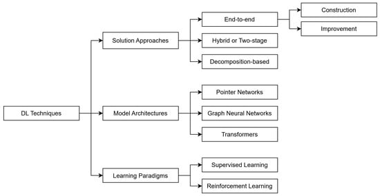
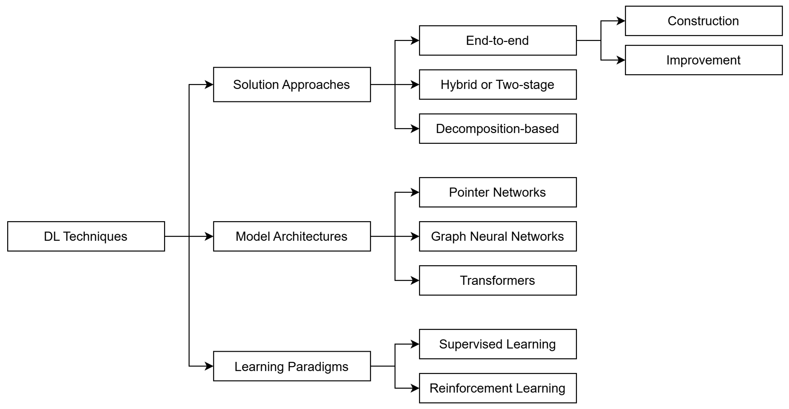
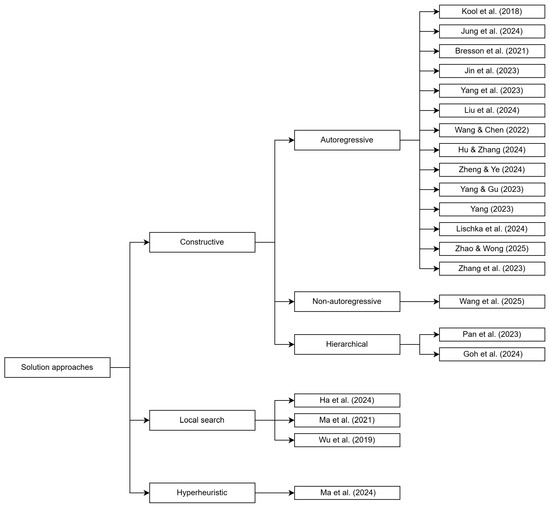
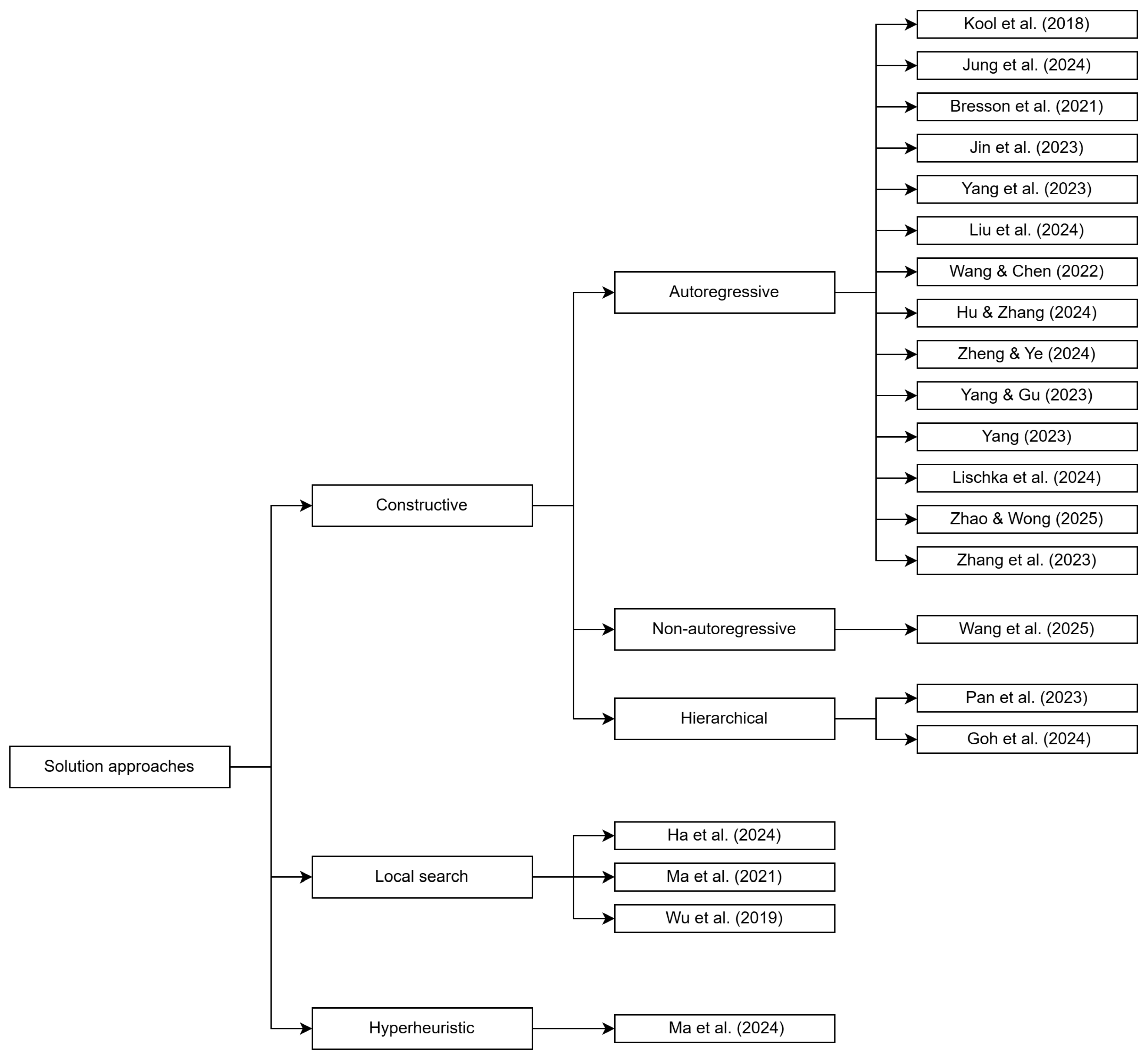
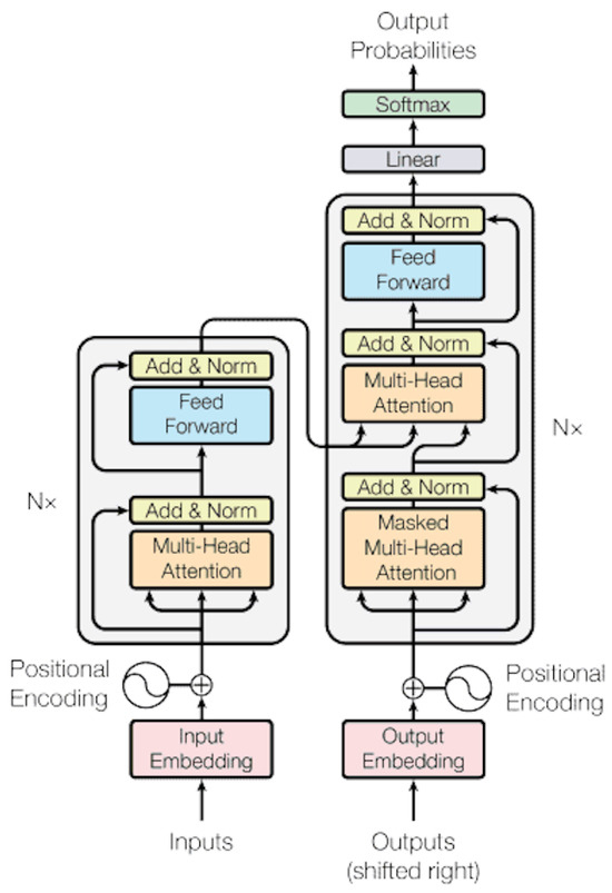
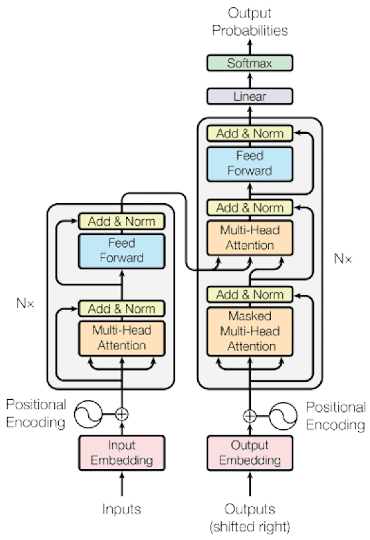
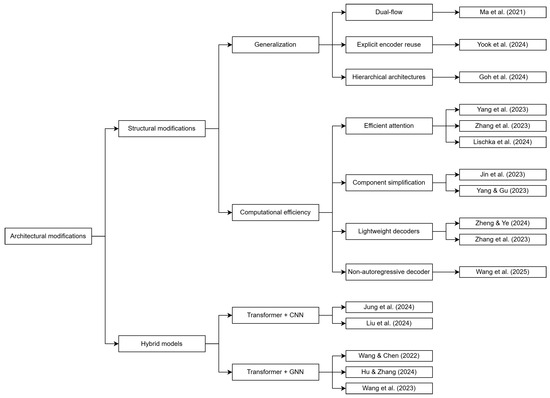
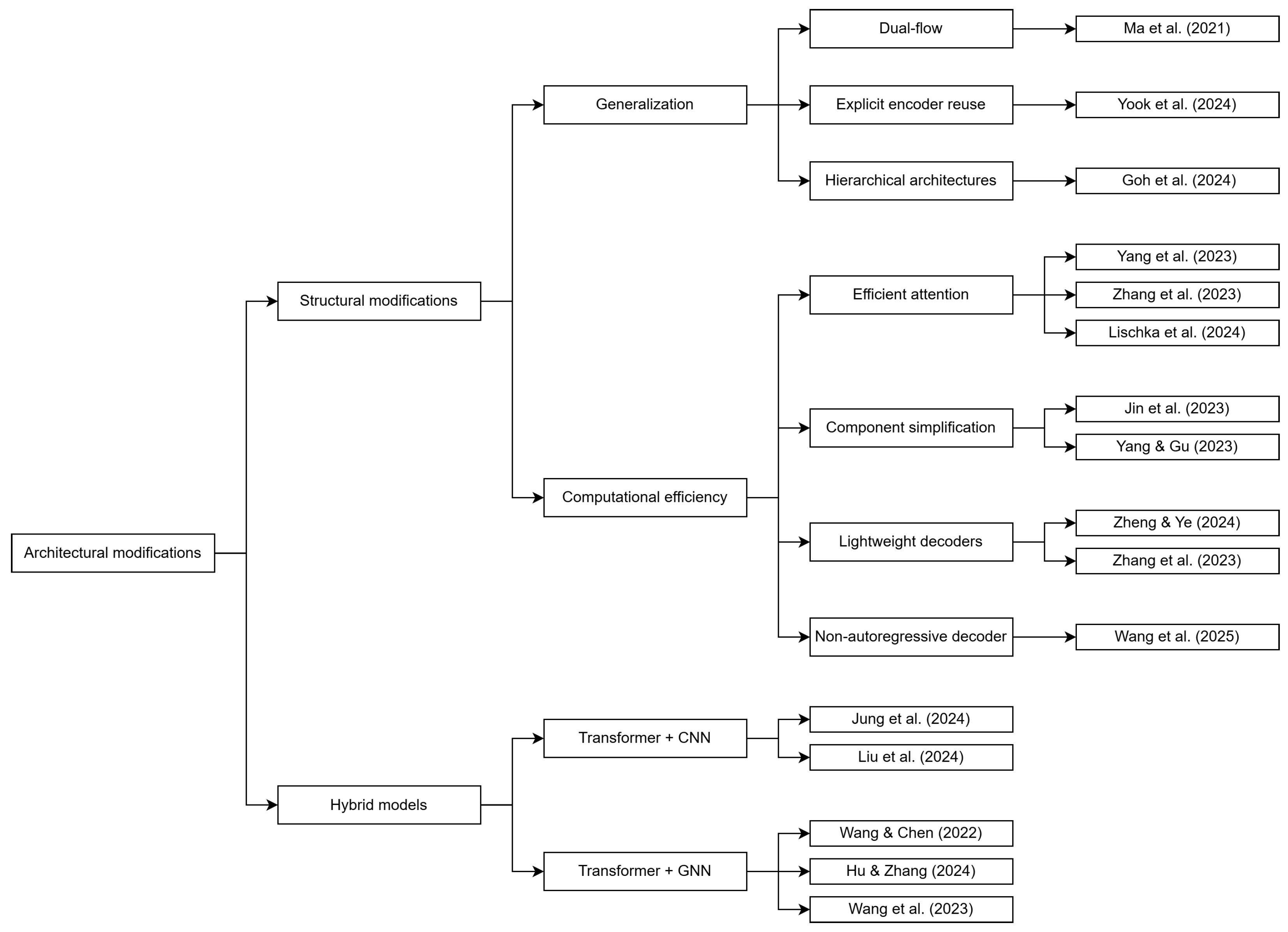
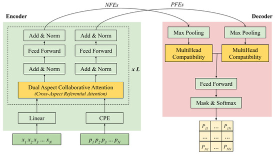
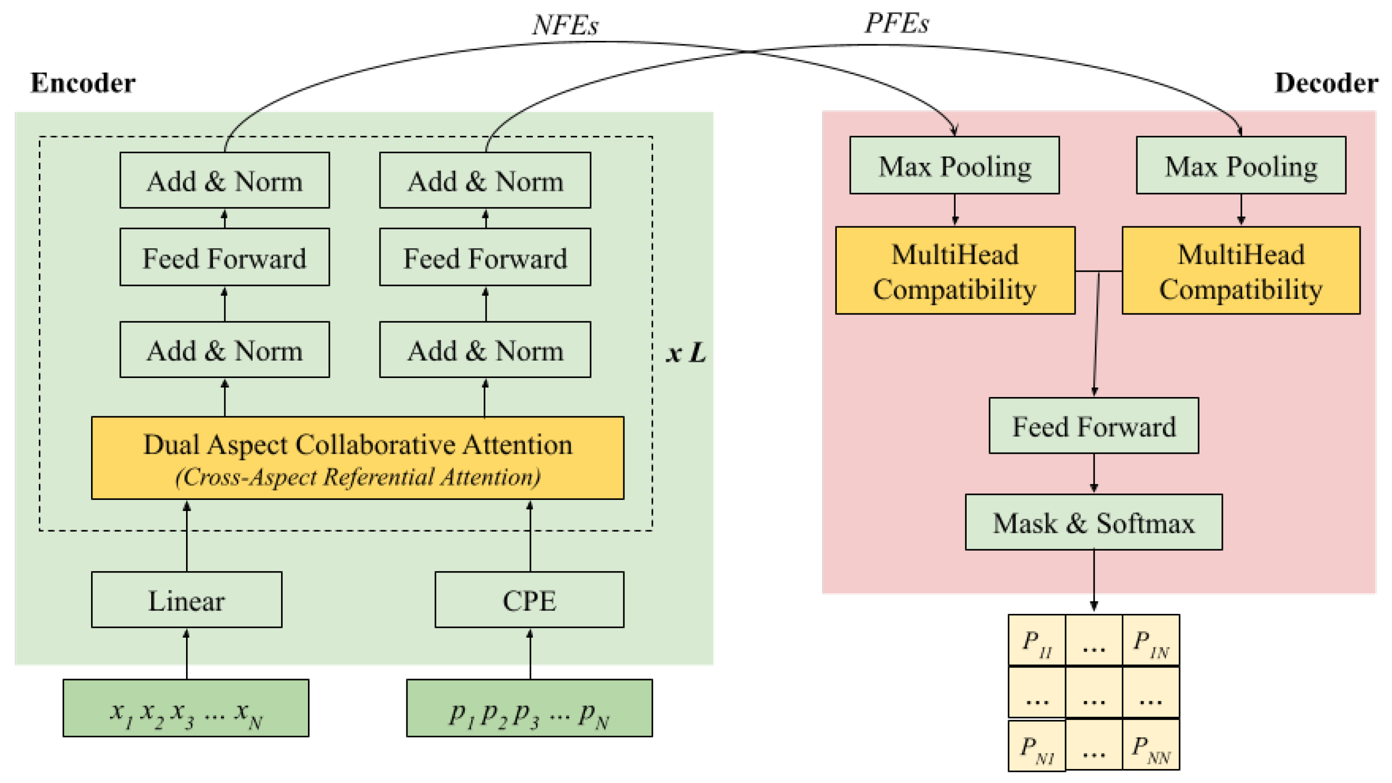
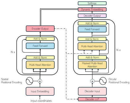
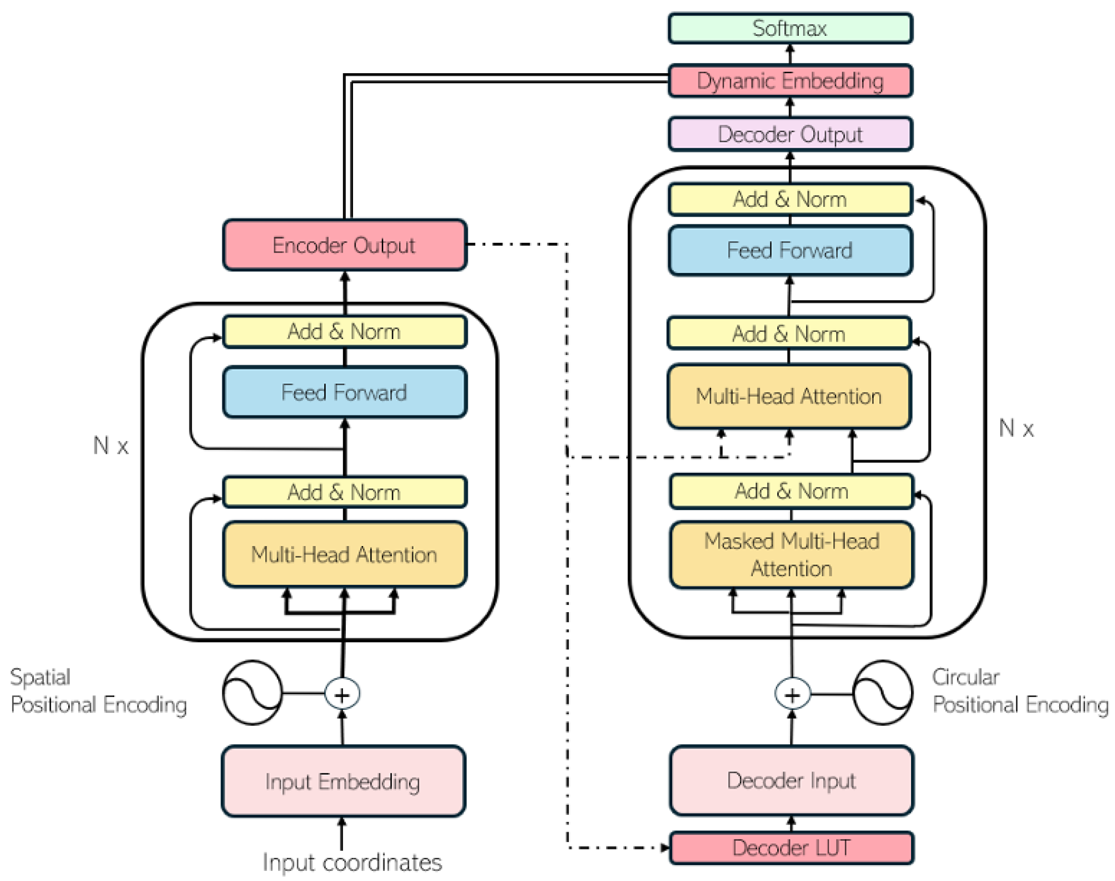
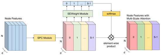
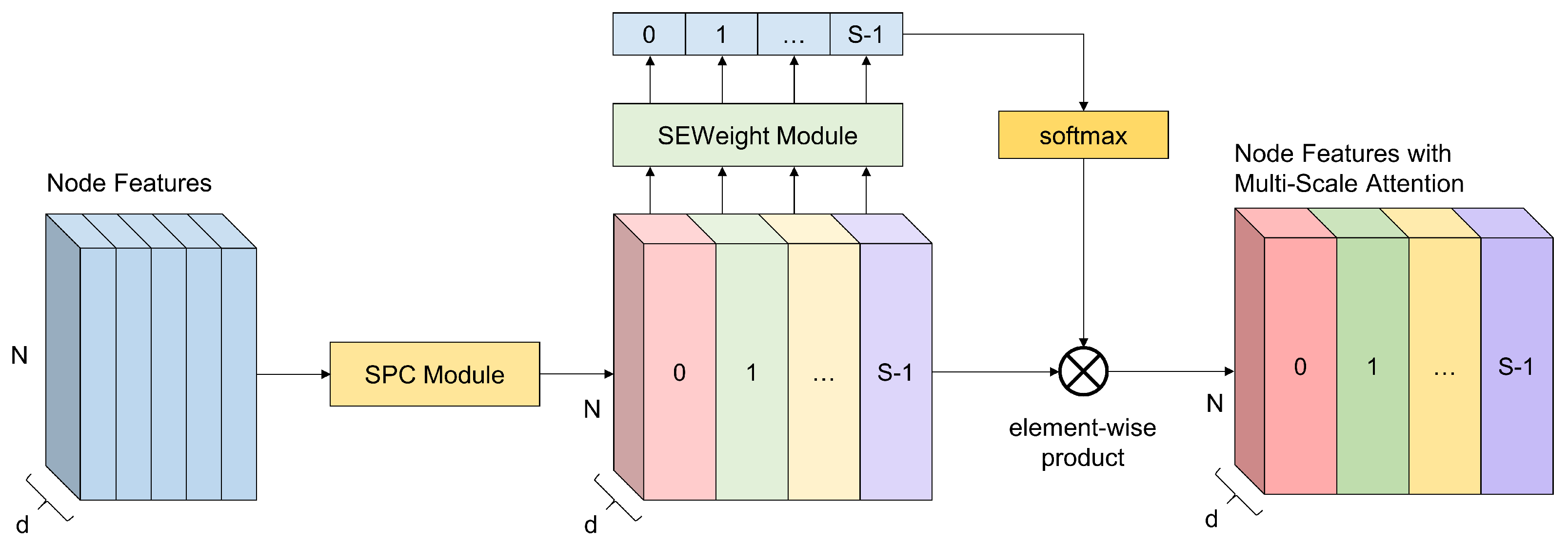
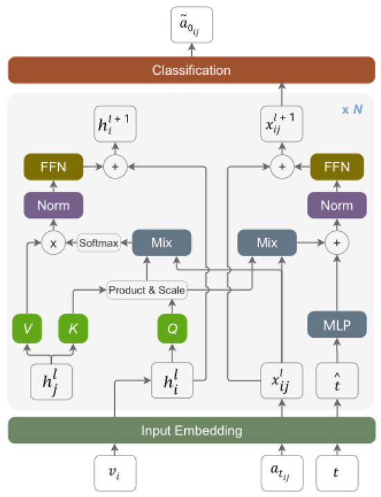
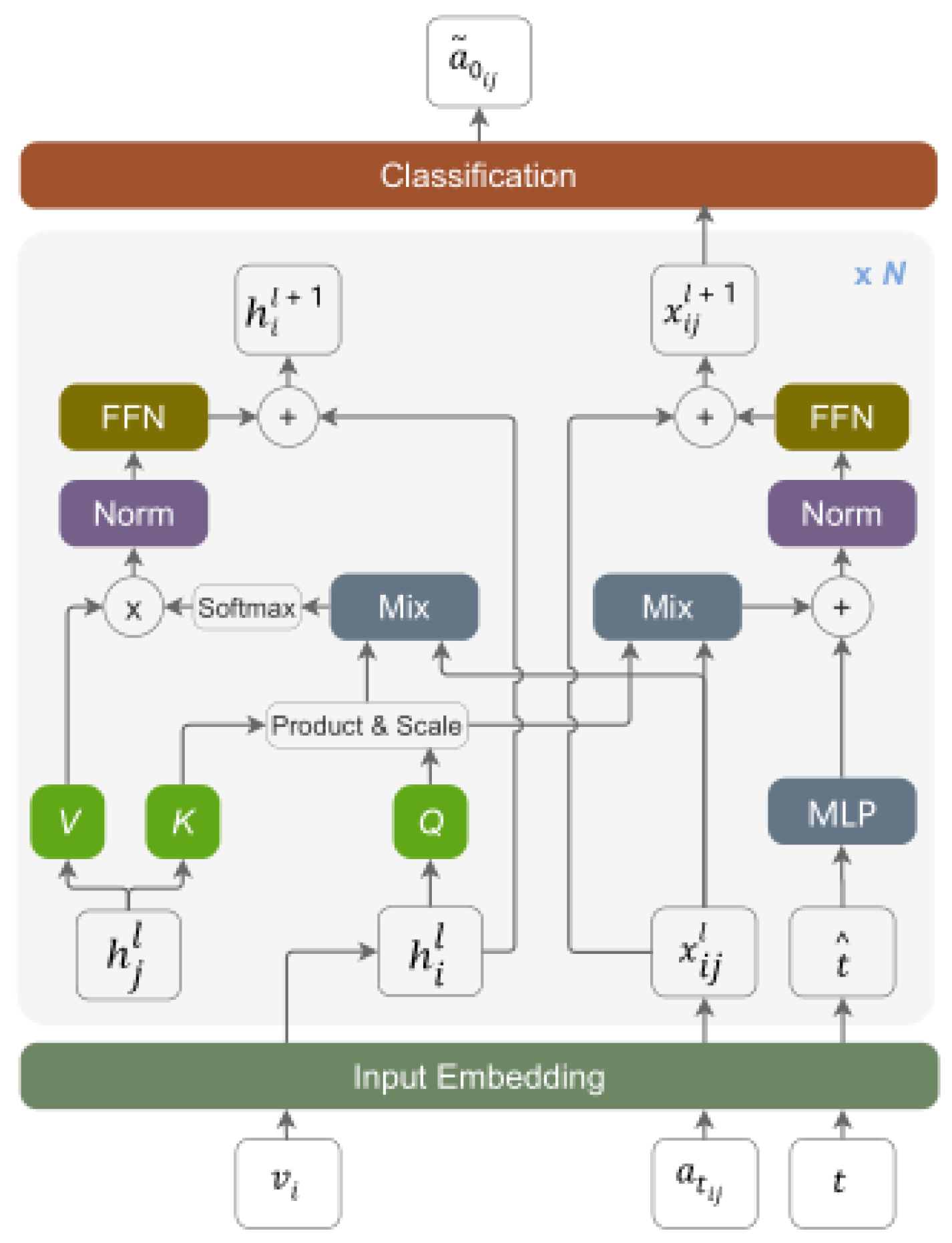
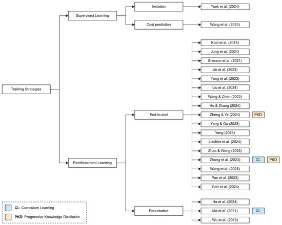
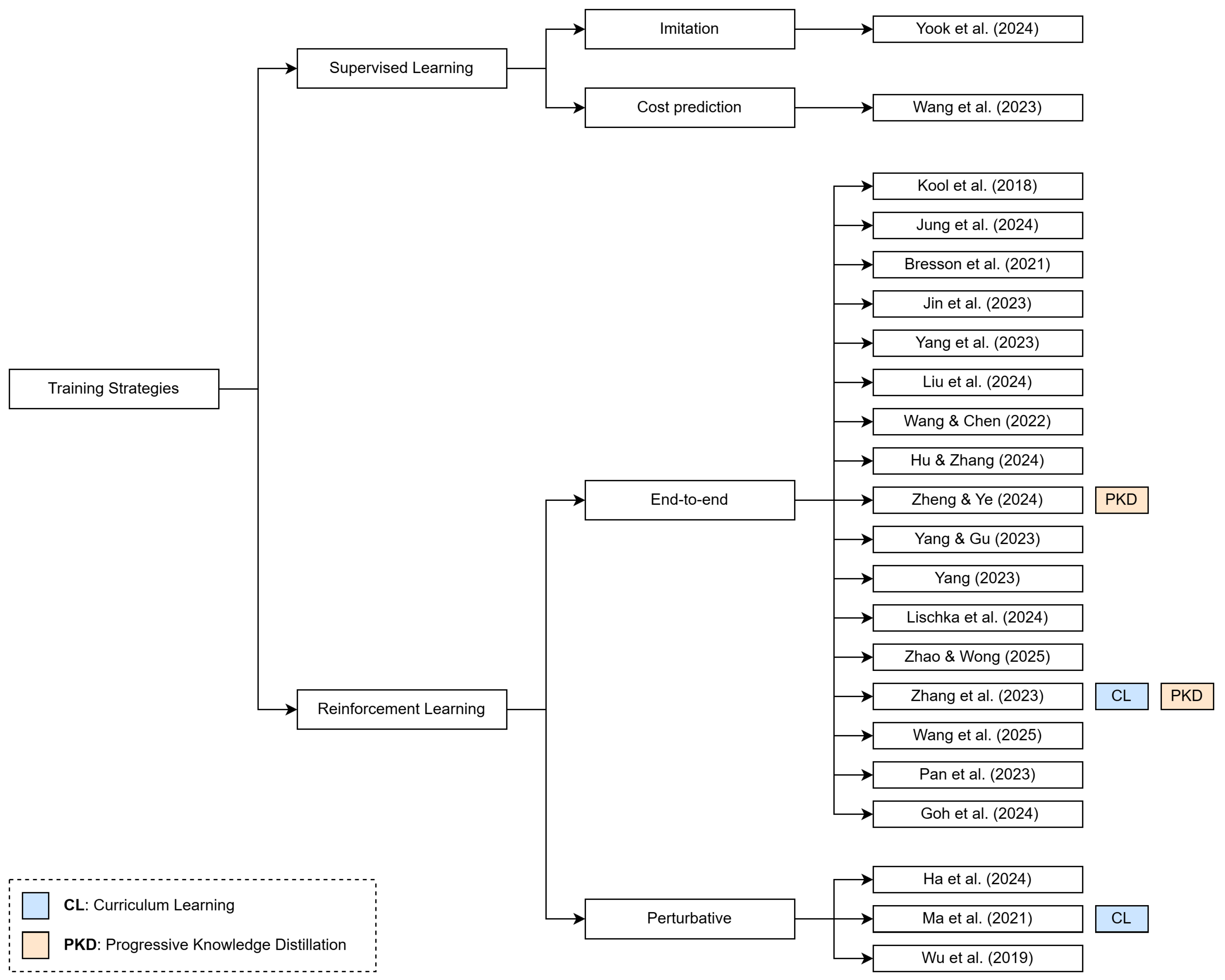
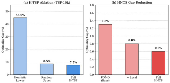
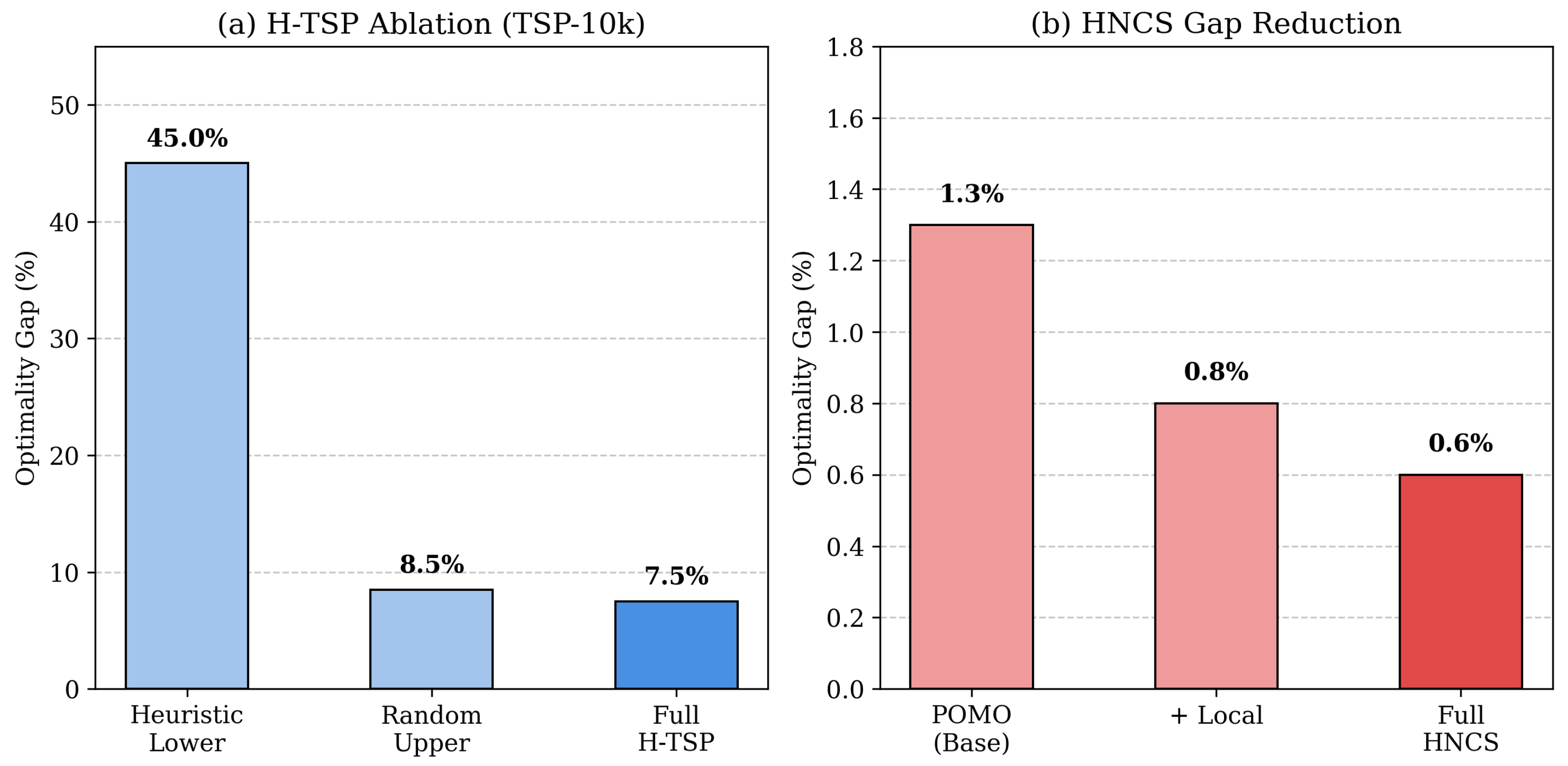

Disclaimer/Publisher’s Note: The statements, opinions and data contained in all publications are solely those of the individual author(s) and contributor(s) and not of MDPI and/or the editor(s). MDPI and/or the editor(s) disclaim responsibility for any injury to people or property resulting from any ideas, methods, instructions or products referred to in the content. |
© 2026 by the authors. Licensee MDPI, Basel, Switzerland. This article is an open access article distributed under the terms and conditions of the Creative Commons Attribution (CC BY) license.