DWARFB: A Dynamic Weight-Adjusted Random Forest Boost for Predicting Financial Distress in Chinese Listed Companies

Abstract

Two key challenges in financial distress prediction are pronounced class imbalance between majority and minority classes and the persistent misclassification of hard-to-learn samples. To tackle these issues, this study proposes an ensemble framework called Dynamic Weight-Adjusted Random Forest Boost (DWARFB). The proposed method incorporates a dynamic sample-weighting mechanism that leverages cumulative misclassification information, adaptive minority–majority class ratios to address class imbalance issue, and a real-time performance-driven strategy to integrate models’ prediction results. The effectiveness of DWARFB is evaluated using a financial dataset from the China Stock Market & Accounting Research (CSMAR) database. Comparative experiments against eight benchmark Random Forest (RF) approaches show that DWARFB delivers superior balanced performance, and a stable precision–recall trade-off, which effectively reduces both false negatives and false positives in the prediction. Moreover, a loss-based feature contribution metric provides economically meaningful insights into the key financial determinants of distress, enhancing model interpretability. Overall, DWARFB demonstrates strong reliability and adaptability and offers a practical solution for early financial distress warning in imbalanced and dynamic financial environments.

1. Introduction

Financial distress is a central concern in model financial risk management, and accurate distress prediction is essential for providing early warnings to companies facing potential bankruptcy or business failure. An effective prediction model typically incorporates finance-related factors such as financial ratios, market indicators, and contextual information to better mitigate financial risk [1]. However, traditional machine learning approaches often struggle with class imbalance and the inherent complexity of financial distress patterns, such as non-linear relationships between liquidity ratios and sudden shifts in company financial health, leading to worse performance [2]. This is largely due to the dynamic nature of financial data, where evolving temporal patterns and shifting economic conditions make accurate prediction more challenging [3]. Therefore, innovative approaches that enhance data utilization beyond traditional financial metrics are essential for more effectively identifying financially distressed companies.

Iterative ensemble methods such as Adaptive Boosting (AdaBoost) and Gradient Boosting have shown promise for addressing such complexities, particularly in imbalanced scenarios [4]. These methods iteratively train base models by adjusting sample weights based on misclassification errors [5]. However, they also suffer from two key limitations: static sample weight adjustment and model inadaptability. AdaBoost relies on fixed exponential rules to update sample weights, which prevent it from recognizing persistent misclassification patterns [6]. This static weighting adjustment scheme cannot adapt post-training and limits its adaptability to handle shifting data distributions [7]. Gradient Boosting, on the other hand, adjusts sample importance for the next model based on the residual errors from the previous iteration, and does not account for samples that are repeatedly misclassified [8]. This makes it less effective at recognizing persistent misclassification patterns. It also assumes a fixed data distribution for all samples and cannot adapt when that distribution changes over time. As a result, it struggles to adapt to dynamic or shifting data. Random Forest (RF), which utilizes the bagging strategy, outperforms many models in financial distress prediction, although it often lacks the ability to adapt to evolving “hardness” of misclassified patterns [9].

Similarly, sample enhancement techniques such as Synthetic Minority Oversampling Technique (SMOTE) and hard sample mining that aim to mitigate class imbalance also lack adaptivity to temporal misclassification history. They treat misclassified samples as static entities and fail to account for the evolving nature of these samples throughout training iterations. For instance, a company with borderline financial health might be misclassified in early iterations but become more predictable with additional lag features, and different sample sets [10]. Shen et al. [11] reported that even after balancing the samples, rigid sample weighting in RF models hinders their ability to capture evolving patterns. Our previously reported findings indicate that no single sampling technique is universally optimal, and the choice of technique should be guided by the specific objectives of the application [12]. We further observed that Bagging-SMOTE and SMOTE–Tomek are more effective for early warning purposes, Tomek Links are useful for reducing false positives in risk-sensitive scenarios, and Random Undersampling (RUS) helps improve computational efficiency.

Two critical research gaps persist in financial distress prediction. Firstly, existing sample enhancement techniques do not incorporate temporal misclassification history. As a result, they fail to amplify the influence of consistently misclassified samples. Secondly, many ensemble methods rely on fixed weight adjustment schemes and neglect the data structure-varying performance of base models. A model that performs well on healthy companies in early iterations may underperform on distressed companies in later stages, and yet its contribution to the final prediction result remains unchanged. These gaps are particularly concerning in high-stakes financial domains, where misclassifying a distressed company as “healthy” can result in substantial investment losses or regulatory penalties [2].

To address these gaps, this study proposes a novel boosting framework to advance financial distress prediction. The framework integrates lagged feature construction to capture temporal dynamics, a dynamic sample-weighting mechanism, adaptive class ratio adjustment, and real-time performance-based model weighting to better account for persistently misclassified samples. RF is selected as the base learner because of its robustness to high-dimensional, correlated financial data and its resilience to overfitting, which is particularly valuable for imbalanced and noisy financial distress datasets [13].

Comprehensive empirical analyses are conducted to rigorously validate the proposed framework’s ability to address these gaps. The effectiveness of the proposed method in handling highly imbalanced financial data and persistently misclassified samples is evaluated through comparisons with eight benchmark RF methods. Performance is evaluated using multiple metrics, including F1-score, precision, recall, Matthews Correlation Coefficient (MCC), and Precision–Recall Area Under the Curve (PR-AUC).

2. Related Works

2.1. Iterative Training Methods

Iterative training methods are widely applied in financial distress prediction. Boosting and bagging represent the two foundational iterative ensemble paradigms, yet they differ fundamentally in adaptability. Boosting reweights errors sequentially, improving sensitivity to minority-class samples, whereas bagging reduces variance through independent learners, but cannot emphasize persistently difficult cases [14]. Although both enhance predictive gains, their rigid designs limit their ability to discriminate against persistent misclassified samples when applied independently. AdaBoost applies exponential weighting to errors within a single iteration [15], which fails to prioritize samples repeatedly misclassified across multiple rounds, leading to poor performance for firms with volatile financial metrics [16]. Meanwhile, Gradient Boosting was designed to fit residual errors sequentially [17] also faces similar constraints as its static learning rates and loss functions struggle to adapting dynamic market conditions [18].

2.2. Sample Enhancement Techniques

Sample enhancement techniques such as hard sample mining have also been widely explored to strengthen model robustness under imbalance and noise. The core idea is to place greater emphasis on samples that are frequently misclassified, thereby refining decision boundaries and improving recall of distressed firms. Common strategies include cost-sensitive learning, which assigns higher penalties to minority-class errors [19], adaptive boosting that reweights misclassified samples across iterations [20], focal loss functions that scale the influence of easy versus hard cases [21], and hybrid sampling strategies that preferentially generate synthetic samples in difficult regions of the feature space [22].

However, most of these approaches reinforce difficult samples only in isolated rounds or through fixed weighting schemes, without tracking cumulative misclassification difficulty over time [23]. This often leaves persistent weaknesses uncorrected, particularly in financial datasets where distress signals are subtle, noisy, and temporally variable. To be effective in such settings, sample enhancement techniques should evolve toward dynamic, history-aware mechanisms that continuously monitor and prioritize persistent difficult cases.

2.3. Ensemble Strategies

Beyond individual sample-level refinements, ensemble models that combine with resampling strategies have gained attention to overcome the rigidity of traditional frameworks. For instance, variants of Adaptive Boosting enhance ensemble adaptability by dynamically reweighting difficult samples, and studies in bankruptcy prediction confirm that combining boosting with resampling strategies such as SMOTE significantly improves minority-class detection [24]. Malek et al. [25] demonstrated that bagging combined with resampling enhanced sensitivity in imbalanced water quality classification, underscoring the complementary strengths of these paradigms. Similarly, Aljawazneh et al. [26] used hybrid SMOTE and Edited Nearest Neighbors (ENNs) within a bagging framework using Support Vector Machines (SVMs) as base learners and reported superior recall and lower Type II error rates compared with conventional deep learning, bagging, and boosting models.

Recent research explored hybrid ensemble strategies that merge boosting’s error-driven weighting with bagging’s diversity, producing more balanced ensembles for complex and imbalanced tasks. These hybrid approaches have demonstrated improved recall of distressed observations. Aljawazneh et al. [27] found that while boosting typically outperforms bagging under severe imbalance, hybrid methods can further improve the predictive performance of financial distress.

Nevertheless, existing flexible ensembles remain limited in their capacity to dynamically adjust to changes in misclassification patterns across iterations. Most current methods rely on single-round adjustments or static ensemble rules, which constrain their ability to respond effectively to evolving data and prevent them from capturing long-term misclassification trends. Addressing this gap requires history-aware, dynamically adaptive architectures capable of reallocating learning resources toward persistently hard samples, thereby improving robustness and generalization in highly imbalanced and noisy financial distress prediction tasks.

Therefore, future hybrid ensemble frameworks should integrate continuous, history-aware adaptation mechanisms that enable the system to adjust learning resources in response to persistent misclassification trends and thereby improve resilience in complex and evolving financial environments.

2.4. Summary of Gaps and Proposed Direction

The reviewed literature on iterative training, sample enhancement, and ensemble strategies highlights three persistent gaps in the context of prediction of financial distress:

(1)

Rigid iterative training

Mainstream boosting methods, such as AdaBoost and Gradient Boosting, employ predefined weight-adjustment rules that overlook cumulative misclassification patterns. Consequently, samples that are consistently misclassified across iterations are not effectively prioritized, limiting the model’s ability to learn from structurally difficult cases.

(2)

Static sample enhancement

Widely used resampling techniques, such as SMOTE and hard sample mining, treat difficult instances as static. They fail to incorporate misclassification history, meaning that once a sample is labeled as “hard,” its importance remains unchanged, regardless of how its classification evolves over time.

(3)

Inflexible ensemble combination

Conventional boosting algorithms combine base learners using fixed weighting mechanisms (e.g., error-based or learning rate-scaled weights). Such static aggregation ignores performance shifts across iterations and reduces robustness when facing evolving and highly imbalanced financial data.

To address these limitations, there is a clear need for an adaptive iterative ensemble framework that integrates three key components:

• Dynamic sample weighting informed by cumulative misclassification history.
• Adaptive sample enhancement where the emphasis on difficult samples evolves with their misclassification frequency.
• Dynamic model combination using cross-validation-driven weight updates rather than fixed rules.

By incorporating history-aware and performance-adaptive mechanisms, the proposed framework aims to improve the generalization and robustness of financial distress prediction models in non-stationary and imbalanced environments.

3. Materials and Methods

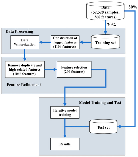
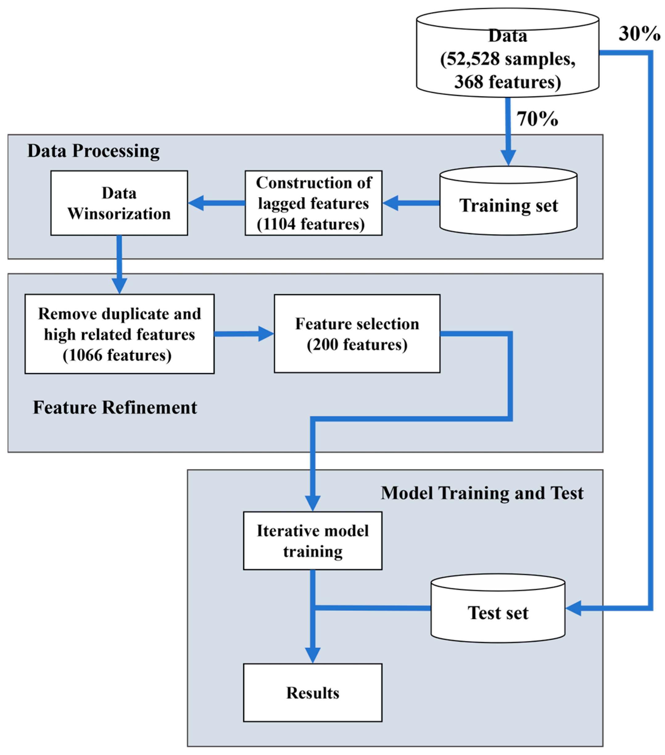
Figure 1 illustrates the schematic workflow of the proposed framework called Dynamic Weight-Adjusted Random Forest Boost (DWARFB). The dataset is first stratified into training and testing sets using the ratio of 70:30. Data preprocessing is then performed on the training data, including lagged features construction, winsorization to reduce the impact of outliers, and the removal of duplicate and highly correlated variables. The cleaned data are trained in the iterative ensemble models. Finally, the prediction performance of the trained classifiers is evaluated using the untouched test data.

Figure 1. The workflow of the proposed framework.

3.1. Data

The dataset used in this study comprised quarterly financial data for 1174 Chinese-listed companies from 2007 to 2024, sourced from the China Stock Market & Accounting Research (CSMAR) database. The data contains 52,528 samples with 368 features, categorized into two distinct classes: distressed and normal. It exhibits a highly imbalanced distribution, with 49,555 samples (94.34%) labeled as normal, and 2973 samples (5.66%) as distressed, resulting in an imbalance ratio of approximately 16.67:1.

3.2. Data Stratification

To ensure robust model evaluation, the data was randomly split into a 70:30 ratio, with 70% of data used for training and the remaining 30% for testing. The split was stratified to maintain the original class imbalance ratio of 16.67:1 in both sets. Consequently, the training set contained 820 companies (36,911 observations, including 2056 distressed samples), and the test set had 354 companies (15,617 observations, including 917 distressed samples). A 5-fold cross-validation was applied during model training, with each fold maintaining the original class imbalance ratio.

3.3. Lagged Feature Construction

The original features were shifted by two and four quarters to construct lagged variables, which were then incorporated as additional features. To prevent look-ahead bias and data leakage, these lagged features were generated separately for the training and test sets. Consequently, the total number of features increased from 368 to 1104. This procedure ensures that no future information is introduced during model training, thereby preserving the temporal ordering and integrity of the data.

3.4. Data Winsorization

To address extreme values in the data without risking the loss of important patterns, we apply Winsorization to handle outliers. Winsorization is a robust statistical technique that mitigates the effect of extreme values by replacing them with the closest values within a specified percentile range, rather than removing them, thereby reducing their impact and preserving the full dataset [28]. In this study, the lower and upper bounds are defined as the 1st ($Q_L$) and 99th ($Q_U$) percentiles, respectively.

Mathematically, for a variable $x_i$:

$$x_i^{Winsorization}=\left\{\begin{array}{c}{Q}_L = if X_i<Q_L\\ Q_U = if X_i>Q_U\\ {\mathrm{x}}_{\mathrm{i}}, \mathrm{otherwise}\end{array}\right.$$

(1)

3.5. Removal of Duplicate Features and Highly Correlated Features

In the first stage, features are compared, and duplicate features, where two features $X_i$ and $X_j$ are identical across all observations $(X_i = X_j)$ are removed. This step eliminates redundant variables that may arise from different variable names representing identical measurements.

In the second stage, Spearman correlation was employed to assess the associations among features. Features with an absolute Spearman correlation coefficient greater than 0.999 were considered highly correlated, and one feature from each highly correlated pair was removed to mitigate multicollinearity. This selection criterion ensures that the most informative feature within each correlated group is retained, aligning with the principle of maximizing feature relevance while minimizing redundancy.

3.6. Feature Selection

Feature selection was conducted using an RF-based importance ranking, where a preliminary model trained on the full feature set assessed predictors by their contribution to reducing prediction error across trees, effectively capturing both linear and non-linear relationships. Validation performance was assessed by increasing the number of top-ranked features. The results show that predictive performance improved as N increased, but gains became marginal beyond approximately 200 features, indicating a performance plateau.

Therefore, a top N strategy with N = 200 was adopted to retain the most informative predictors while balancing predictive power, computational efficiency, and interpretability. To prevent data leakage, feature importance was computed on the training set only, and the same subset was applied to the test set.

3.7. Iterative Ensemble Algorithm

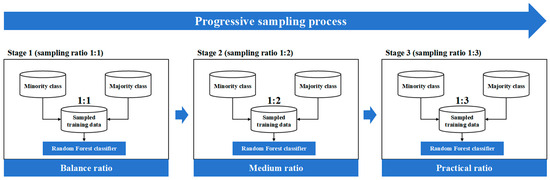
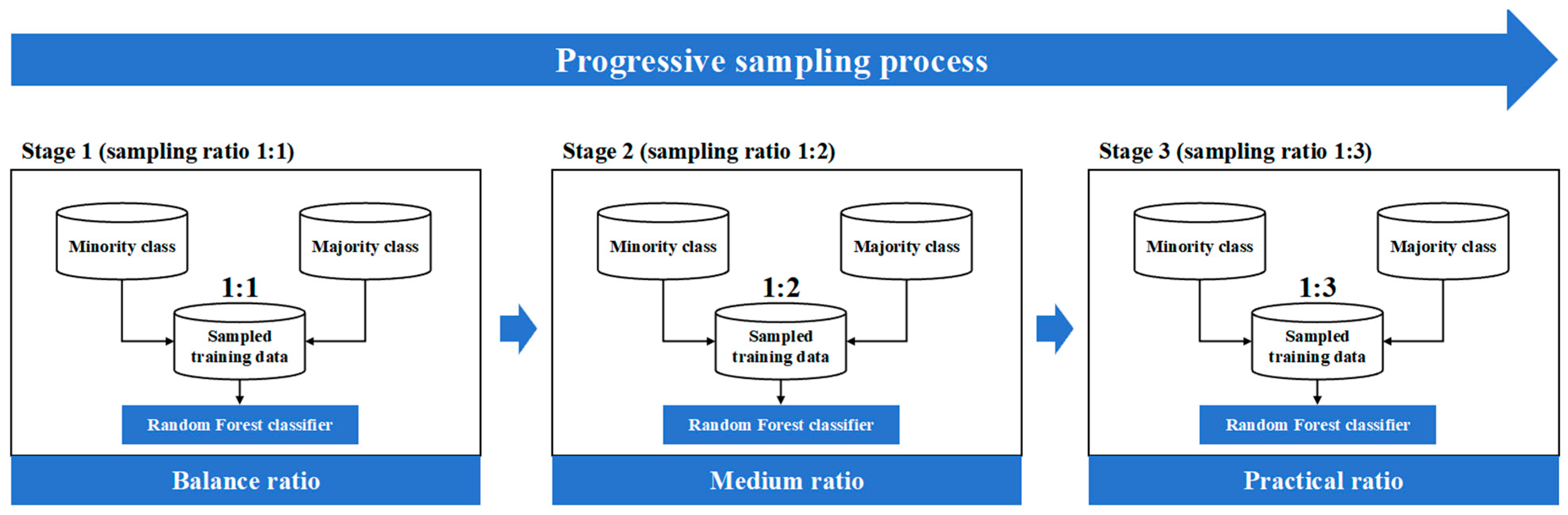
In the proposed model, the process begins by training an RF model on the first subset of the training data. All distress samples are selected in each of the subsets. All misclassified samples from this subset are recorded, and in subsequent iterations, these misclassified normal samples are prioritized for selection in the next training subset. This iterative training process is repeated until no further improvement is observed in the cross-validation F1-score. Figure 2 depicts the multi-stage sampling process carried out in an iterative environment.

Figure 2. The multi-stage sampling process in the iterative environment.

Each stage uses a different positive-to-negative sample ratio. Initially, a 1:1 ratio is applied, which is then progressively adjusted to 1:2 and 1:3 in subsequent stages. For each sampling stage, the entire training process is repeated, generating multiple subsets, each containing all available positive samples (i.e., distress samples in this study) and a selectively chosen portion of negative samples (i.e., normal samples in this study). Noteworthy that the selection of negative samples prioritizes those misclassified in earlier iterations, enabling the model to focus on hard-to-classify cases. This iterative, ratio-based training approach helps each model specialize in different aspects of the data, particularly in recognizing complex distress patterns.

During model training, a separate RF model is trained for each subset. The outputs from these models are then integrated using an adaptive, performance-driven ensemble strategy to produce the final prediction. The final ensemble model is evaluated on the test set, and adaptive thresholding is applied to determine the optimal classification boundary.

3.7.1. Minority–Majority Ratio Adjustment Strategy

To tackle the class imbalance issue in the multi-stage sampling process, we employ a dynamic class adjustment strategy, referred to as the minority–majority ratio adjustment. This approach progressively increases the difficulty of the classification task by gradually introducing more majority-class samples during training, transitioning from a balanced to an imbalanced setting.

In each iteration process, all minority samples (i.e., distressed samples) are included in every training subset, while majority samples (i.e., normal samples) are selected based on a predefined sampling ratio. Majority samples that were misclassified in the previous iteration are given higher priority for inclusion in the current training subset. The remaining quota is filled by randomly selecting from the pool of majority samples that have never been misclassified. The objective is to enable the model to adapt to varying class ratios and ultimately identify “gray” samples, i.e., samples that are consistently misclassified by the model. The sample selection is expressed as follows pseudocode (Algorithm 1).

Algorithm 1. The Strategy of Sample Selection

INITIALIZE: $\mathrm{Include} \mathrm{all} \mathrm{positive} \mathrm{samples} \mathrm{in} \mathrm{every} \mathrm{iteration}: S_{\mathrm{pos}}\leftarrow P$ Set misclassification counters for all negative samples $\mathbf{FOR} \mathrm{each} \mathrm{iteration} t = 1$$\mathrm{to} T$DO Compute required number of negatives: $${\mathrm{r}\mathrm{e}\mathrm{q}\mathrm{u}\mathrm{i}\mathrm{r}\mathrm{e}\mathrm{d}}_{\mathrm{n}\mathrm{e}\mathrm{g}} = \mathrm{m}\mathrm{i}\mathrm{n}(\mid N\mid ,\mid P\mid \times (\mathrm{neg}\_\mathrm{ratio}/\mathrm{pos}\_\mathrm{ratio}\left)\right)$$ Select negative samples: $\mathrm{Prioritize} \mathrm{negatives} \mathrm{misclassified} \mathrm{in} \mathrm{iteration} t-1$: ▪ $N_{\mathrm{mis}}\leftarrow \{x\in N\mid x \mathrm{misclassified} \mathrm{in} t-1\}$ ▪ $k_1\leftarrow \mathrm{m}\mathrm{i}\mathrm{n}(\mid N_{\mathrm{mis}}\mid ,\mathrm{required}\_\mathrm{neg})$ ▪ $S_{\mathrm{neg}1}\leftarrow$$\mathrm{select} \mathrm{top} k_1$$\mathrm{from} N_{\mathrm{mis}}$ Fill remaining quota from all negative samples: ▪ $k_2\leftarrow \mathrm{required}\_\mathrm{neg}-k_1$ ▪ $S_{\mathrm{neg}2}\leftarrow$$\mathrm{randomly} \mathrm{select} k_2$$\mathrm{from} N\setminus N_{\mathrm{mis}}$ $S_{\mathrm{neg}}\leftarrow S_{\mathrm{neg}1}\cup S_{\mathrm{neg}2}$ Form training subset: $S^{\left(t\right)}\leftarrow S_{\mathrm{pos}}\cup S_{\mathrm{neg}}$ $\mathbf{Train} \mathbf{model} \mathrm{on} S^{\left(t\right)}$ $\mathbf{Update} \mathbf{misclassification} \mathbf{history} M^{\left(t\right)}$ using predictions on full training pool END FOR OUTPUT: $\mathrm{Training} \mathrm{subsets} S^{\left(t\right)}$ $\mathrm{Misclassification} \mathrm{history} M^{\left(T\right)}$ “Gray” samples identified as consistently misclassified

3.7.2. Misclassified Sample Weight Enhancement Mechanism

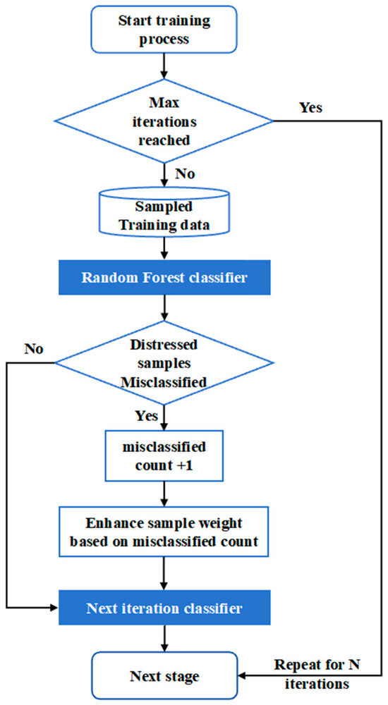
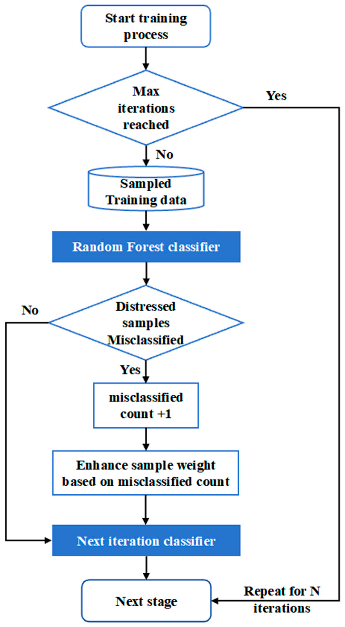
To effectively handle hard samples that are consistently misclassified across multiple training iterations, we introduced a novel weight enhancement mechanism (see Figure 3). This mechanism combines concepts from meta-learning and reward/penalty-based schemes to adaptively increase the focus on these challenging instances. The mathematical formulation of this approach is presented in Equation (2).

Figure 3. The misclassified sample weight enhancement process.

The sample weight for each sample is computed using a multi-component formula that combines exponential scaling with threshold-based boosting.

$$w_i^{\left(mis\right)}=1+\alpha {\left({\displaystyle \frac{{mis}_i}{\mathit{max}\left({mis}_{max},1\right)}}\right)}^{\gamma }+\alpha \times I\left(mi{s}_i \ge threshold\right)$$

(2)

where $w_i^{\left(mis\right)}$ is the weight for sample $i$, ${mis}_i$ is the misclassification count for sample $i$, ${mis}_{max}$ is the maximum misclassification count across all samples, $threshold$ is the 80% of misclassification counts (i.e., the top 20% most difficult samples), $\alpha$ and $\gamma$ are weight adjustment parameters, and $I(.)$ is the indicator function that equals 1 when the condition is met, 0 otherwise.

The additional reward factor adaptively reduces the weights of samples once they are correctly predicted over consecutive iterations, preventing permanent inflation. The final weights are calculated as follows:

$$w_{final}={\mathrm{w}}_{\mathrm{i}}^{\left(\mathrm{m}\mathrm{i}\mathrm{s}\right)}\times rewar{d}_{factor}$$

(3)

The hyperparameters $\alpha$ and $\gamma$ were determined via grid search with cross-validation on the training set. Specifically, the search ranges were defined as:

$$\alpha \in \{\mathrm{2,4},\mathrm{6,8},\mathrm{10,12,15}\},\gamma \in \{\mathrm{1,2},\mathrm{3,4},\mathrm{5,6}\}.$$

The optimal configuration was selected based on the highest cross-validation F1-score. The best performance was achieved at $\alpha =15$ and $\gamma =1$.

This formulation integrates three complementary ideas. The progressive re-weighting of misclassified samples follows the intuition of AdaBoost [29]. The power term $\gamma$ resembles the focusing mechanism on Focal Loss [30], which adjusts the strength of weight amplification. Finally, the threshold indicator reflects the concept of hard example mining [31], ensuring that persistently misclassified cases receive additional reinforcement. Unlike existing approaches, our approach provides a unified weighting strategy that simultaneously incorporates linear scaling, non-linear focusing, and discrete reinforcement, thereby enhancing the robustness of ensemble learning for imbalanced financial distress prediction.

3.7.3. Integrating Prediction Results Using Performance-Driven Assessment Strategy

In conventional RF integration, prediction results from each trained model are simply averaged to produce the final output. This method treats all trained models equally, without considering their individual predictive performance. As a result, poorly performing models may degrade the overall performance of the ensemble. To alleviate this issue in our study, we propose an adaptive, performance-driven assessment strategy. The proposed performance-driven approach continuously monitors cross-validation performance metrics and dynamically adjusts model weights based on real-time F1-score feedback. The objective of the proposed approach is to facilitate fine-grained ensemble control and strengthen the model’s capacity to sustain optimal integration performance.

(1)

Adaptive Model Weight Adjustment

The F1-scores of previously trained models are logit-transformed and the corresponding weight ${\alpha }_t$ is calculated as:

$${\alpha }_{\mathrm{t}}=\log \left({\displaystyle \frac{{F1}_t}{1-F{1}_t+\epsilon }}\right)$$

(4)

where $\mathrm{F}{1}_{\mathrm{t}}$ represents the cross-validation F1-score of model trained at iteration t, and $\epsilon$ is a small constant (1 × 10⁻⁸) introduced to prevent division by zero. This transformation ensures that higher-performing models receive exponentially larger weights while maintaining numerical stability.

Using the logit-transformed weight ${\alpha }_t$ and a scoring value $f\left(x\right)=\{0.5,0.8,1.2,2.0\}$ representing the actual F1-score obtained in each iteration, a new weight $w_i$ is computed as follows:

$$w_i = {\alpha }_t\ast f\left(x\right)$$

(5)

where

$$f\left(x\right)=\left\{\begin{array}{l}0.5, \mathrm{if} \mathrm{F}{1}_{\mathrm{t}}\ge 0.85 (\mathrm{Very} \mathrm{high} \mathrm{performance})\\ 0.8, \mathrm{if} 0.80\le \mathrm{F}{1}_{\mathrm{t}}<0.85 (\mathrm{High} \mathrm{performance})\\ 1.2, \mathrm{i}\mathrm{f} 0.75\le \mathrm{F}{1}_{\mathrm{t}}<0.80 (\mathrm{Satisfactory} \mathrm{performance})\\ 2.0, \mathrm{if} \mathrm{F}{1}_{\mathrm{t}}<0.75 (\mathrm{Low} \mathrm{performance})\end{array}\right.$$

To ensure numerical stability and prevent dominance by extreme weights, the computed weights were scaled and serve as the distance of the input to the target classes.

$$\widehat{w_i}={\displaystyle \frac{w_i}{\sum _{i=1}^T{w}_i }}$$

(6)

This approach assigns different levels of influence to the predicted samples based on their distance from different target classes. Samples closer to a target class are given higher weights while farther samples contribute to the respective class.

(2)

Compute Prediction Probability

Using the updated weights $\widehat{W} = \{\widehat{w_1,} \widehat{w_2,}\dots , \widehat{w_T}\}$, the prediction score for each target class $\mathrm{c}$ is computed:

$$\mathrm{S}\mathrm{c}\mathrm{o}\mathrm{r}\mathrm{e}\left({\mathrm{C}}_{\mathrm{k}}\right)={\sum }_{i=1}^t\widehat{w_i}$$

(7)

where $C_k$ denotes the summation of the sample weight $x_i$ from each iteration $t$ to the class $k$. The final classification decision is obtained by selecting the class with the highest total weight.

$$\widehat{y}=\mathrm{a}\mathrm{r}\mathrm{g} \underset{C}{\max } \mathrm{S}\mathrm{c}\mathrm{o}\mathrm{r}\mathrm{e}\left(C\right)$$

(8)

3.7.4. Optimal Classification Threshold Selection

To improve classification performance under class imbalance, the decision threshold is adaptively optimized rather than fixed at 0.5.

Let $P(y=1\mid x)$ denote the predicted probability of financial distress produced by the ensemble model. For a given threshold $\tau \in \left[\mathrm{0,1}\right]$, the binary prediction is defined as:

$${\widehat{y}}_{\tau }\left(x\right)=\left\{\begin{array}{cc}1,& \mathrm{if} P(y=1\mid x)\ge \tau ,\\ 0,& \mathrm{otherwise}.\end{array}\right.$$

(9)

The optimal threshold ${\tau }^{*}$ is selected by maximizing the F1-score on the validation set:

$${\tau }^{*}=\mathrm{a}\mathrm{r}\mathrm{g}\underset{\tau \in \left[\mathrm{0,1}\right]}{\mathrm{m}\mathrm{a}\mathrm{x}}F1(\tau )$$

(10)

Here, $F1\left(\tau \right)$ denotes the F1-score computed using predictions ${\widehat{y}}_{\tau }\left(x\right)$. The search is conducted over a grid of threshold values within $\left[\mathrm{0,1}\right]$.

Finally, the optimized threshold ${\tau }^{*}$ is applied to the ensemble probability outputs to generate the final classification results.

This adaptive thresholding strategy ensures that the decision boundary is aligned with the performance objective under class imbalance, thereby improving the balance between precision and recall compared to a fixed 0.5 threshold.

3.8. Experimental Design

Firstly, a comparison experiment is conducted, where DWARFB is benchmarked against various RF models using a 5-fold cross-validation. The predictive performance of the models is evaluated using test data. A statistical significance analysis is then performed to validate the robustness of the models. Each experiment is repeated 20 times with different random seeds, and results are examined using the Wilcoxon signed-rank test (α = 0.05), F1-based ranking, and 95% confidence intervals. The hyperparameters such as number of trees, maximum depth, minimum split size, and minimum leaf size are analyzed to assess RF robustness under different configurations.

3.8.1. Evaluation Metrics

(1)

Cohen’s Kappa

Cohen’s Kappa coefficient [32] is a robust measure of classification reliability that adjusts for chance agreement, offering advantages over accuracy in imbalanced datasets. It is defined as:

$$\kappa = {\displaystyle \frac{P_o - P_e}{1 - P_e}},$$

(11)

where $P_o$ is the observed agreement (accuracy) and $P_e$ is the expected agreement by chance, derived from the confusion matrix. For binary classification,

$$P_e={\displaystyle \frac{\left(TP+FP\right)\left(TP+FN\right)+(TN+FN)(TN+FP)}{N^2}}$$

(12)

Interpretation typically ranges from poor ($\kappa <0.2$) to almost perfect agreement ($\kappa \ge 0.8$). Given its sensitivity to class imbalance, Cohen’s Kappa provides a more reliable evaluation of financial distress prediction models than accuracy alone.

(2)

Feature Importance

We employed a loss-based feature contribution metric to measure how much each feature reduces the weighted misclassification loss during the DWARFB training process. A feature is considered important if it consistently leads to a large reduction in classification loss across boosting iterations. The loss-based feature importance for feature $f$ is defined as:

$$F{I}_f = {\displaystyle \frac{\sum _{t=1}^T{\alpha }_t(L^{\left(t−1\right)} - L_f^{\left(t\right)})}{\sum _k\sum _{t=1}^T{\alpha }_t(L^{\left(t−1\right)} - L_k^{\left(t\right)})}}$$

(13)

where:

$T$ is the total number of boosting iterations.

$f$ denotes a specific feature, and $k$ indexes all features.

$L^{\left(t-1\right)}$ is weighted classification loss before the $t$-th iteration.

$L_f^{\left(t\right)}$ is the loss after the splits involve feature $f$ at iteration $t$.

${\alpha }_t$ is the boosting weight of the $t$-th base learner.

This metric provides a performance-driven and interpretable measure of feature importance in the context of financial distress prediction.

3.8.2. Classification Evaluation

Multiple performance metrics were used to examine prediction performance of the model. Table 1 outlines the metrics used in this study with F1-score designated as the primary optimization criterion.

Table 1. Classification evaluation metrics used in the experiment.

Metric	Formula	Description
Precision	${\displaystyle \frac{\mathrm{T}\mathrm{P}}{\mathrm{T}\mathrm{P}+\mathrm{F}\mathrm{P}}}$	Proportion of correctly predicted positive samples among all predicted positives
Recall	${\displaystyle \frac{\mathrm{T}\mathrm{P}}{\mathrm{T}\mathrm{P}+\mathrm{F}\mathrm{N}}}$	Proportion of correctly predicted positive samples among all actual positives
F1-score	${\displaystyle \frac{2\times \mathrm{P}\mathrm{r}\mathrm{e}\mathrm{c}\mathrm{i}\mathrm{s}\mathrm{i}\mathrm{o}\mathrm{n}\times \mathrm{R}\mathrm{e}\mathrm{c}\mathrm{a}\mathrm{l}\mathrm{l}}{\mathrm{P}\mathrm{r}\mathrm{e}\mathrm{c}\mathrm{i}\mathrm{s}\mathrm{i}\mathrm{o}\mathrm{n}+\mathrm{R}\mathrm{e}\mathrm{c}\mathrm{a}\mathrm{l}\mathrm{l}}}$	Harmonic mean of precision and recall
ROC-AUC	${\int }_0^1\mathrm{T}\mathrm{P}\mathrm{R}\left(\mathrm{F}\mathrm{P}\mathrm{R}\right)\mathrm{d}\left(\mathrm{F}\mathrm{P}\mathrm{R}\right)$	Area under the Receiver Operating Characteristic curve
PR-AUC	${\int }_0^1\mathrm{P}\mathrm{r}\mathrm{e}\mathrm{c}\mathrm{i}\mathrm{s}\mathrm{i}\mathrm{o}\mathrm{n}\left(\mathrm{R}\mathrm{e}\mathrm{c}\mathrm{a}\mathrm{l}\mathrm{l}\right)d\left(Recall\right)$	Area under the Precision–Recall curve
MCC	${\displaystyle \frac{\left(\mathrm{T}\mathrm{P}\times \mathrm{T}\mathrm{N}\right)-(\mathrm{F}\mathrm{P}\times \mathrm{F}\mathrm{N})}{\sqrt{(\mathrm{T}\mathrm{P}+\mathrm{F}\mathrm{P})(\mathrm{T}\mathrm{P}+\mathrm{F}\mathrm{N})(\mathrm{T}\mathrm{N}+\mathrm{F}\mathrm{P})(\mathrm{T}\mathrm{N}+\mathrm{F}\mathrm{N})}}}$	Matthews Correlation Coefficient measures overall binary classification quality

$\mathrm{T}\mathrm{P}$ denotes True Positive, $\mathrm{T}\mathrm{N}$ denotes True Negative, $\mathrm{F}\mathrm{P}$ is False Positive, $\mathrm{F}\mathrm{N}$ is False Negative, $\mathrm{T}\mathrm{P}\mathrm{R}$ is True Positive Rate (i.e., recall), and $\mathrm{F}\mathrm{P}\mathrm{R}$ is False Positive Rate.

3.8.3. Wilcoxon Signed-Rank Test

The Wilcoxon signed-rank test [33] is a non-parametric alternative to the paired t-test. It was used to assess whether performance differences between models were statistically significant across cross-validation folds. Unlike parametric tests, it does not assume normality of metric distributions and is robust to outliers and skewed results.

Formally, for paired scores $x_i$ and $y_i$, differences $d_i=x_i-y_i$ are computed, with zero values excluded. The absolute differences $\mid d_i\mid$ are ranked, and the sums of positive $W^{+}$ and negative $W^{-}$ ranks are obtained. The test statistics are defined as follows:

$$W =\mathrm{m}\mathrm{i}\mathrm{n} (W^{+},W^{-})$$

(14)

which, for sufficiently large $n$, is approximated by a normal distribution:

$$Z ={\displaystyle \frac{W -\frac{n(n+1)}{4}}{\sqrt{\frac{n(n+1)(2n+1)}{24}}}}$$

(15)

A p-value of 0.05, corresponding to a 95% confidence level, was used as the threshold to reject the null hypothesis, indicating that the performance improvements are statistically significant.

4. Result Analysis and Discussion

4.1. Predictive Performance of DWARFB

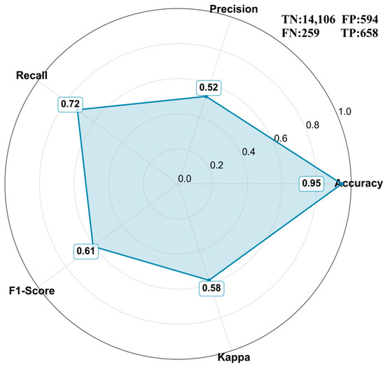
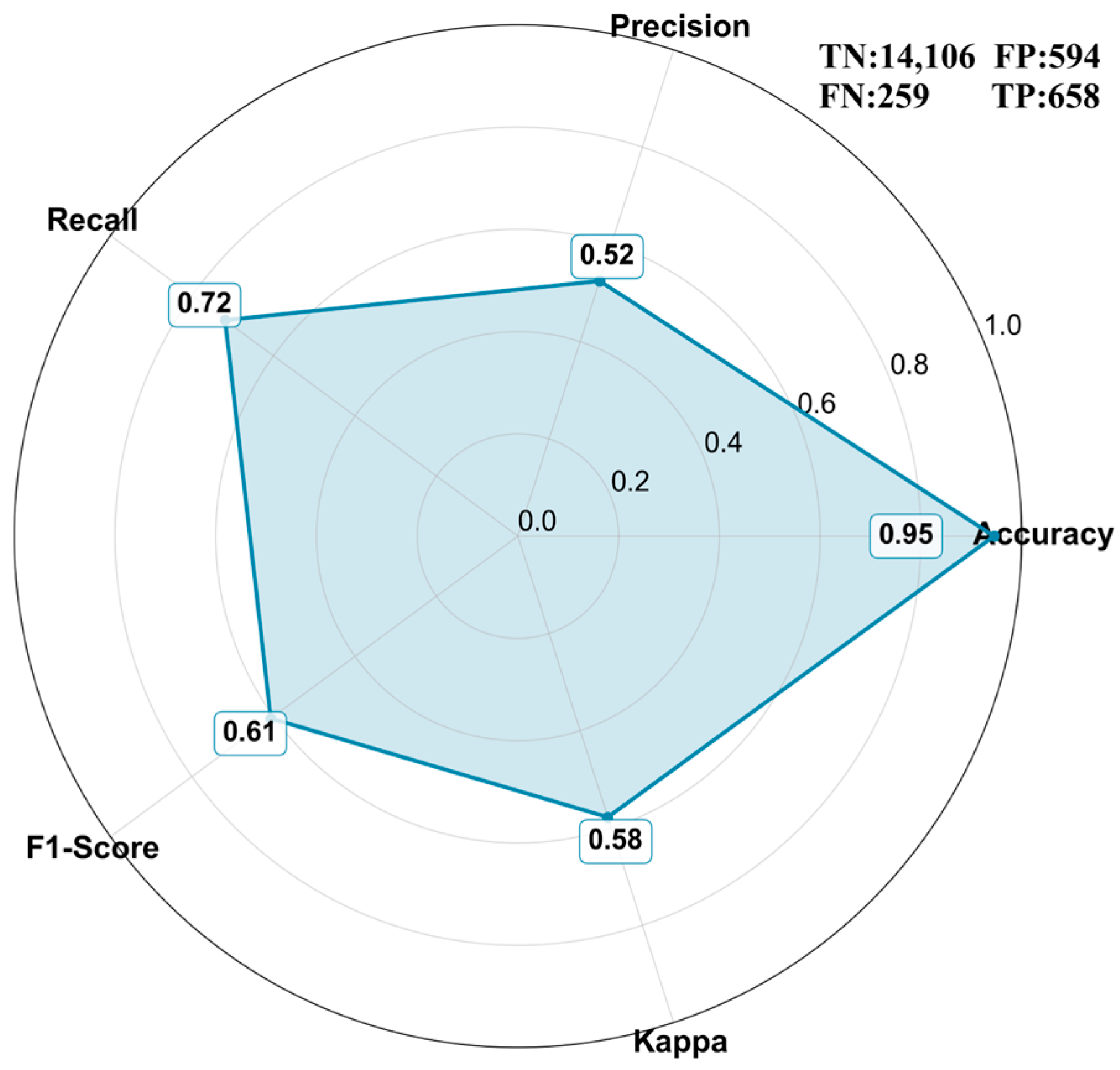
The evaluation results presented in Figure 4 provide a comprehensive view of the predictive performance of DWARFB in the context of financial distress detection. The high overall accuracy of 0.95 suggests that the model possesses strong discriminative capability. However, given the severe class imbalance inherent in financial datasets, accuracy is a limited indicator of model reliability. A more nuanced interpretation is revealed through metrics such as precision, recall, F1-score, and Cohen’s Kappa.

Figure 4. The performance radar chart of DWARFB.

DWARFB achieves a recall of 0.72, indicating its capacity to correctly identify a substantial proportion of distressed samples. This is a favorable outcome in risk-sensitive applications, where missing a distressed sample (false negative, FN) may have far-reaching financial and managerial consequences. The relatively low number of FN (i.e., 259 out of 917 distressed cases, ~0.28) produced by the model reflects its ability to prioritize sensitivity, thereby supporting its suitability for early warning purposes.

At the same time, the relatively modest precision of 0.52 in Figure 4 suggests that nearly half of the samples flagged as distressed are, in fact, financially healthy. Although the trade-off between precision and recall is typical in imbalanced classification problems, the presence of 594 false positives may introduce potential inefficiencies by increasing the burden of follow-up investigations. From a practical perspective, this could translate into unnecessary resource allocation by regulators, investors, or creditors, thereby limiting the model’s operational efficiency.

The F1-score of 0.61 demonstrates that the model achieves a balanced compromise between precision and recall, although the balance leans slightly toward sensitivity rather than specificity. Similarly, Cohen’s Kappa value of 0.58 falls within the range of moderate agreement, underscoring that the model’s discriminative ability is not solely a function of the majority class but reflects meaningful performance across both classes. Importantly, the discrepancy between high accuracy and moderate Kappa illustrates the pitfalls of relying on accuracy in imbalanced domains and highlights the necessity of employing multiple evaluation criteria.

Taken together, these results indicate that DWARFB provides a solid baseline for financial distress prediction. Its strength lies in reducing the risk of overlooking distressed samples, which aligns with the conservative requirements of financial risk management. Nonetheless, the relatively high false positive rate signals the need for further refinement, particularly in enhancing precision without sacrificing recall.

4.2. Benchmarking Against Random Forest (RF) Baseline Models

Table 2 summarizes the comparative performance of DWARFB and various RF baseline approaches, achieved from 20 independent experiments. The inclusion of multiple trials ensures that the reported performance is not the outcome of random fluctuations but reflects stable and reproducible patterns.

Table 2. Performance comparison of baseline methods.

Method	F1-Score	Precision	Recall	MCC	Accuracy	Training Time (in Seconds)
Standard RF	0.51 ± 0.02	0.75 ± 0.02	0.38 ± 0.02	0.52 ± 0.02	0.96 ± 0.00	28.6
Cost-sensitive RF	0.57 ± 0.01	0.60 ± 0.01	0.55 ± 0.02	0.55 ± 0.01	0.95 ± 0.00	49.0
Balanced RF	0.46 ± 0.01	0.31 ± 0.01	0.89 ± 0.01	0.48 ± 0.01	0.87 ± 0.00	3.5
RF + RUS	0.45 ± 0.01	0.30 ± 0.01	0.88 ± 0.01	0.47 ± 0.01	0.87 ± 0.01	1.7
RF + SMOTE	0.56 ± 0.01	0.44 ± 0.01	0.76 ± 0.01	0.54 ± 0.01	0.93 ± 0.00	67.0
RF + Borderline SMOTE	0.56 ± 0.01	0.44 ± 0.01	0.76 ± 0.01	0.54 ± 0.01	0.93 ± 0.00	51.0
RF + ADASYN	0.55 ± 0.01	0.42 ± 0.01	0.77 ± 0.01	0.54 ± 0.01	0.92 ± 0.00	50.9
RF + SMOTE Tomek	0.56 ± 0.01	0.45 ± 0.01	0.74 ± 0.01	0.55 ± 0.01	0.93 ± 0.00	60.8
DWARFB	0.62 ± 0.01	0.58 ± 0.04	0.67 ± 0.05	0.60 ± 0.01	0.95 ± 0.00	387.9

Across all evaluation metrics, DWARFB demonstrates superior consistency and overall predictive balance. Specifically, DWARFB achieves the highest F1-score (0.62 ± 0.01) and MCC (0.60 ± 0.01), clearly outperforming all baselines. The observed performance ranges further indicate that the method yields robust and stable performance across repeated runs. In contrast, the Standard RF, while delivering the highest accuracy (0.96) and precision (0.75 ± 0.02), exhibited relatively larger variability in precision. More critically, its low recall (0.38 ± 0.02) reveals a persistent bias toward the majority class, leading to frequent misclassification of distressed samples. Cost-sensitive RF provided a more even trade-off, raising recall to 0.55 ± 0.02 with a moderate F1-score of 0.57 ± 0.01. However, it was consistently surpassed by DWARFB in terms of both F1-score and MCC. Similarly, resampling-based approaches (RF + SMOTE, RF + Borderline SMOTE, RF + ADASYN, and RF + SMOTE Tomek) displayed improved recall values (0.74–0.77), but their reduced precision (0.42–0.45) constrained overall performance, reflected in lower F1-scores (0.55–0.56).

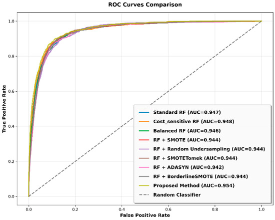
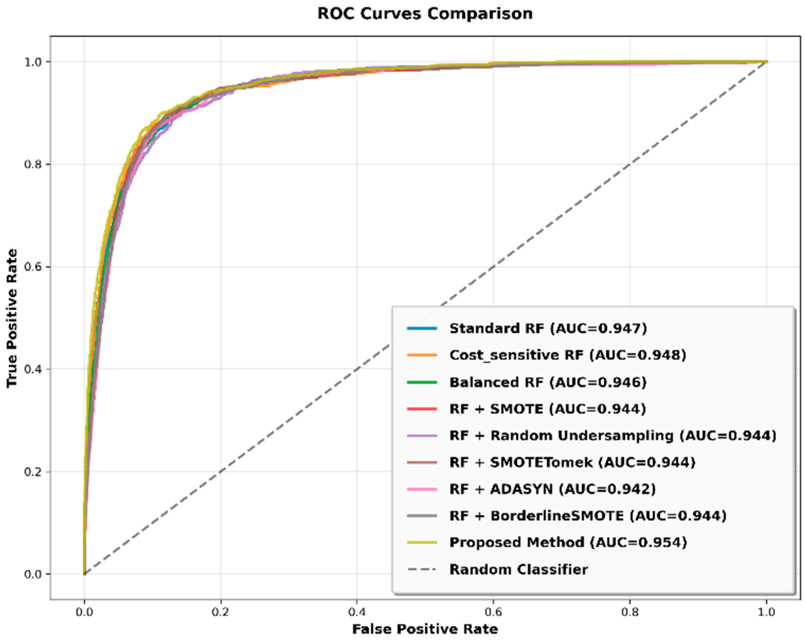
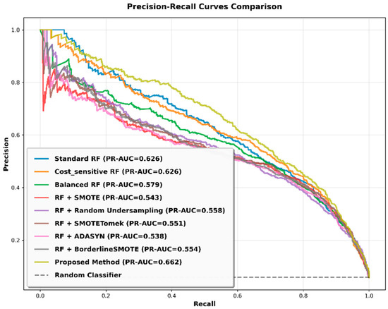
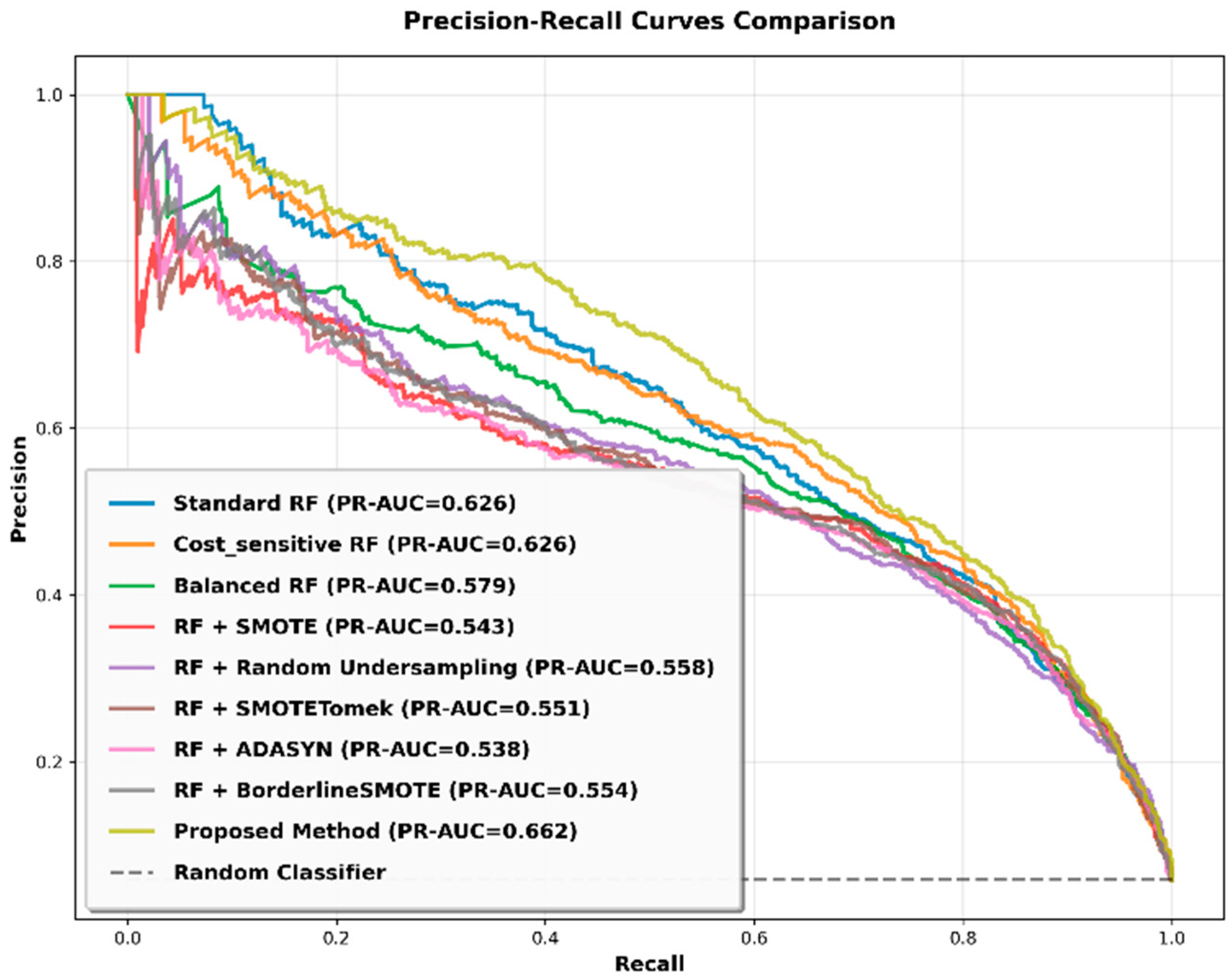
Analyses of the ROC and PR curves further show that DWARFB achieves a well-balanced trade-off between precision and recall in distress detection. Figure 5 shows that DWARFB achieved the highest ROC-AUC (0.954), outperforming the strongest baseline (Cost-sensitive RF, 0.948). Although the numerical gain appears modest, the consistently higher ROC curve across multiple false positive rate intervals indicates genuine improvement rather than random noise. More importantly, the PR curves (see Figure 6) emphasize robustness in imbalanced settings, with DWARFB achieving the highest PR-AUC (0.662).

Figure 5. ROC curve comparison.

Figure 6. Precision–Recall (PR) curve comparison.

Methods emphasizing under-sampling, such as Balanced RF and RF + RUS, yielded the highest recall (0.89 ± 0.01 and 0.88 ± 0.01, respectively) but drastically reduced precision (~0.31 ± 0.01 and ~0.30 ± 0.01, respectively). This imbalance produced the lowest F1-scores (0.44–0.46) and the greatest variability in precision, demonstrating that overly aggressive minority emphasis undermines reliability. By contrast, DWARFB maintains a balanced trade-off between precision (0.58 ± 0.04) and recall (0.67 ± 0.05), ensuring that both types of misclassifications are controlled within reasonable bounds.

The main limitation of DWARFB is its computational cost, with a training time of 387.9 s (see Table 2), substantially higher than the baselines. This overhead primarily occurs during the offline training phase due to the iterative boosting mechanism and dynamic misclassification history updates. In practical early financial warning systems, model training is conducted periodically (e.g., quarterly), whereas prediction is performed frequently. Importantly, the inference complexity of DWARFB remains comparable to other tree-based ensemble models, ensuring that large-scale real-time risk screening is not affected.

From an operational perspective, a training time of approximately 6.5 min remains computationally feasible for institutional environments. Given the high-stakes nature of financial distress prediction, the improvement in classification performance, particularly the reduction in false negatives, justifies the moderate increase in computational cost.

Furthermore, the additional overhead is largely parallelizable. Efficiency can be enhanced through parallel cross-validation, parallel tree construction, GPU acceleration, distributed training frameworks, and adaptive early stopping strategies, thereby improving scalability for large-scale deployment.

In summary, the comparative results demonstrate that DWARFB consistently delivers superior and stable classification performance. Its balanced precision and recall make it particularly suitable for financial distress prediction, where the consequences of missed detections far exceed the costs of additional false alarms.

4.3. Statistical Significance Analysis

To rigorously evaluate whether the observed improvements of DWARFB over baseline classifiers are statistically significant, we conducted pairwise Wilcoxon signed-rank tests across the 20 independent experimental runs. This non-parametric test was selected because it makes no assumption of normality and is particularly suited for comparing paired performance results across repeated experiments.

Table 3 summarizes the results, reporting p-values, effect sizes (Cohen’s d), and the corresponding performance differences (ΔF1 and ΔAUC). Across all comparisons, DWARFB consistently and significantly outperformed baseline approaches (all p-values < 0.001), with Cohen’s d values ranging from 8.63 to 42.47. These values correspond to extremely large effects under conventional thresholds, confirming that the observed differences are not only statistically significant but also practically meaningful.

Table 3. Pairwise Wilcoxon test results comparing DWARFB with benchmark models.

Benchmark Model	p-Value	Effect Size	ΔF1	ΔAUC
Standard RF	<0.001	15.59	0.107	0.006
Cost-sensitive RF	<0.001	8.63	0.036	0.005
Balanced RF	<0.001	42.47	0.153	0.007
RF + SMOTE	<0.001	11.23	0.053	0.010
RF + RUS	<0.001	32.58	0.165	0.010
RF + SMOTE Tomek	<0.001	12.89	0.054	0.011
RF + ADASYN	<0.001	14.35	0.064	0.011
RF + Borderline SMOTE	<0.001	11.24	0.050	0.010

From the perspective of performance metrics, the following is observed:

• ΔF1: DWARFB demonstrates substantial gains in F1-score relative to all baselines, with improvements ranging from +0.036 (vs. Cost-sensitive RF) to +0.165 (vs. RF + RUS). These results confirm its superior capability to balance precision and recall, especially compared to under-sampling approaches, which suffer from very high variance and loss of precision.
• ΔAUC: Although absolute improvements in AUC are relatively modest (between +0.005 and +0.011), the consistent gains across all comparisons are noteworthy, particularly given that all baseline AUC values were already above 0.94. Even such marginal increases in AUC can translate into meaningful improvements in real-world financial distress prediction, where early detection of additional distressed firms can significantly reduce losses.
• Largest Improvements: The most notable gains are observed against Balanced RF (ΔF1 = +0.153, d = 42.47) and RF + RUS (ΔF1 = +0.165, d = 32.58). These results highlight the ability of DWARFB to avoid the pitfalls of over-aggressive under-sampling, which inflates recall at the expense of precision.

Collectively, these findings reinforce the conclusions of the previous section, where DWARFB not only achieves higher performance across metrics but also delivers statistically reliable and practically significant improvements. The combination of large effect sizes, consistent gains across both F1 and AUC, and robustness over 20 experimental runs provides strong empirical evidence of its superiority for financial distress prediction.

4.4. Parameters of Base Learner

To evaluate the impact of base learner hyperparameter settings on the performance of DWARFB, 15 combinations of four core hyperparameters in RF are examined. These hyperparameters are n_estimators, max_depth, min_samples_split, and min_samples_leaf. Table 4 summarizes the performance of DWARFB across these hyperparameters.

Table 4. The overall performance based on various combinations of parameters.

N_Estimators	Max_Depth	Min_Samples_Split	Min_Samples_Leaf	CV_F1 Mean	CV_Precision Mean	CV_Recall Mean	CV_MCC Mean
50	10	2	10	0.70	0.62	0.80	0.68
50	10	5	1	0.72	0.65	0.81	0.70
50	10	10	1	0.71	0.64	0.80	0.70
50	10	10	10	0.70	0.61	0.80	0.68
50	15	5	10	0.70	0.62	0.80	0.69
100	5	5	5	0.63	0.54	0.76	0.61
100	10	2	10	0.70	0.63	0.79	0.68
100	10	10	1	0.71	0.64	0.80	0.69
100	15	2	1	0.74 *	0.66 *	0.82 *	0.72 *
100	15	2	5	0.72	0.64	0.81	0.70
150	5	5	5	0.63	0.54	0.75	0.61
150	10	2	1	0.71	0.64	0.80	0.70
150	10	5	1	0.72	0.66	0.80	0.71
150	10	10	1	0.71	0.64	0.80	0.70
150	15	10	10	0.71	0.63	0.81	0.70

* Bold indicates the best performance. CV denotes cross-validation.

As shown in Table 4, predictive performance of DWARFB is significantly influenced by these hyperparameters. The F1-score varies from 0.63 to 0.74, the average recall ranges from 0.75 to 0.82, and the MCC spans from 0.61 to 0.72. Precision shows the greatest variability, ranging from a low of 0.54 to 0.66.

The best-performing configuration was observed with 100 estimators, max_depth = 15, min_samples_split = 2, and min_samples_leaf = 1, achieving highest predictive performance with precision of 0.66, F1-score of 0.74, recall of 0.82, and MCC of 0.72. In contrast, shallow trees (i.e., max_depth = 5) consistently underperformed, with F1-scores dropping to 0.63 and MCC to 0.61, indicating limited representational capacity.

To better isolate the contribution of each parameter, the cross-validated results were regrouped by single-parameter values (see Table 5). The aggregated means reveal the following patterns:

Table 5. Iterative model performance by single parameter grouping.

Parameter	Setting Value	Num.	F1-Score Mean	Precision Mean	Recall Mean	MCC Mean	Training Time (in Seconds) Mean
N_Estimators	50	5	0.71	0.63	0.80	0.69	688.03
	100	5	0.70	0.62	0.80	0.68	1394.25
	150	5	0.70	0.62	0.79	0.68	1992.35
Max_Depth	5	2	0.63	0.54	0.76	0.61	1229.22
	10	9	0.71	0.64	0.80	0.69	1392.34
	15	4	0.72	0.64	0.81	0.70	1358.85
Min_Samples_Split	2	5	0.71	0.64	0.80	0.70	1542.54
	5	5	0.68	0.60	0.78	0.66	1255.08
	10	5	0.71	0.63	0.80	0.69	1200.94
Min_Samples_Leaf	1	7	0.72	0.65	0.80	0.70	1508.22
	5	3	0.66	0.57	0.77	0.64	1379.92
	10	5	0.70	0.62	0.80	0.69	662.09

• Max Depth: Exerts the strongest influence, with mean F1-score rising from 0.63 (depth = 5) to 0.72 (depth = 15), a 14.2% relative improvement.
• Min Samples Leaf: A leaf size of 1 delivers the best performance (F1-score = 0.72, MCC = 0.70), while larger leaves degrade predictive granularity.
• Min Samples Split: Exhibits a U-shaped effect, very low (2) and relatively high (10) values perform better than intermediate values (5).
• N Estimators: Has marginal impact on predictive accuracy (F1-score ≈ 0.70–0.71) but significantly increases training time (from 688 s at 50 estimators to 1992 s at 150 estimators).

These findings highlight several important insights into model behavior and practical implications:

(1)

Depth and granularity dominate discriminative power

The substantial performance gains from increasing Max Depth and minimizing leaf size suggest that random forest benefits from capturing highly non-linear and detailed decision boundaries. This is especially critical in imbalanced financial distress prediction, where subtle signals distinguish distressed firms from the majority non-distressed cases.

(2)

Trade-off between generalization and overfitting

While deeper trees (Max Depth = 15) improve F1-score and recall, the risk of overfitting may increase in smaller or noisier datasets. However, in this study’s large-scale financial dataset, deeper models appear to generalize well, as evidenced by consistent MCC improvements.

(3)

Split threshold flexibility matters

The U-shaped effect of Min Samples Split indicates that both very permissive and relatively strict splitting strategies support better tree structures, while moderate thresholds constrain growth, leading to reduced model expressiveness.

(4)

Efficiency vs. marginal accuracy gains

Increasing the number of estimators has diminishing returns for predictive accuracy but substantially inflates computational cost. From a cost–benefit perspective, 50–100 estimators strike the optimal balance between efficiency and robustness, which is relevant for real-world financial applications requiring timely risk detection.

4.5. Convergence Behavior and Penalty Weight Stability of DWARFB

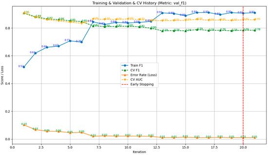
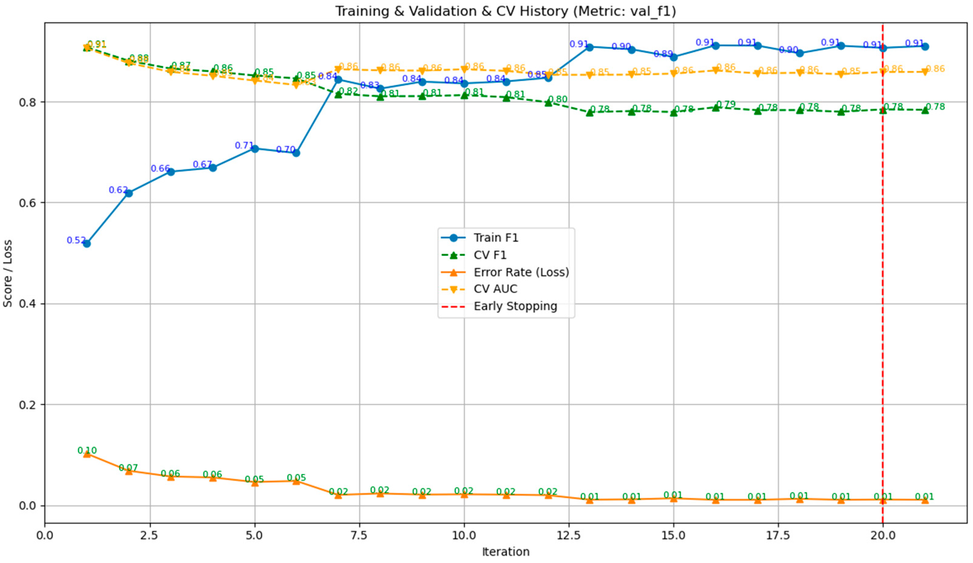
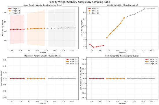
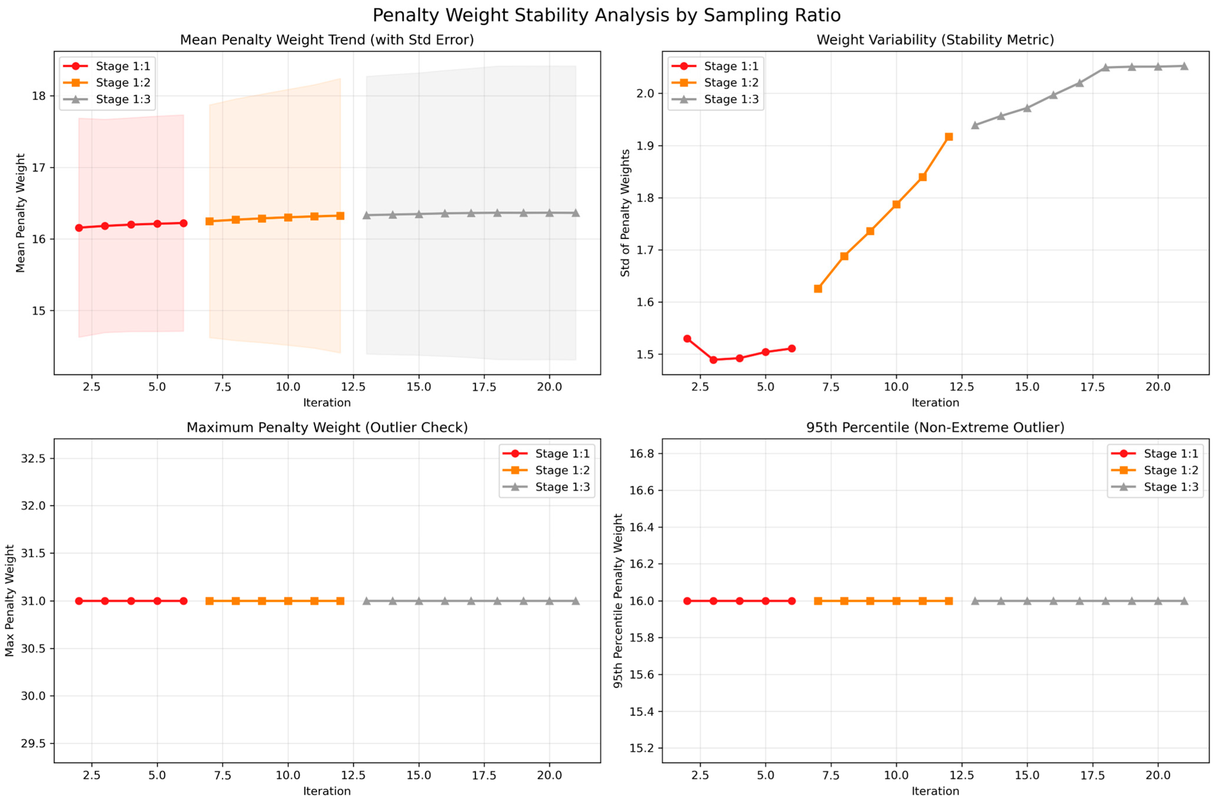
Figure 7 and Figure 8 illustrate DWARFB’s convergence and the stability of penalty weights under the adaptive sampling strategy and penalty weight adjustment.

Figure 7. Convergence behavior of the DWARFB model.

Figure 8. Penalty weight stability analysis by sampling ratio.

Initially, with a 1:1 minority-to-majority ratio, the training F1-score rises sharply, and classification loss drops, showing rapid correction of early misclassifications. When the validation F1-score stagnates for five iterations, the sampling ratio is adjusted to 1:2, then 1:3 if needed. This reduces minority overrepresentation, aligning training with realistic class distributions. As a result, cross-validation F1 shows a slight, temporary decrease, reflecting the trade-off between minority discrimination and overall generalization. After adjustments, training F1 continues to improve moderately, while validation F1 and AUC remain stable, and loss plateaus without oscillation, confirming robust convergence.

Penalty weights for minority samples remain controlled throughout all stages (Figure 8). At 1:1, the mean weight is ~16.2 with low variability (SD < 1.52). At 1:2, the mean slightly rises to ~16.3 (SD ~1.92), reflecting nuanced reweighting. At 1:3, the mean stabilizes at ~16.35 with SD ~2.05, indicating bounded variability. Maximum weights (~31.0) and 95th percentiles (~16.0) remain flat across all iterations, confirming the absence of extreme or non-extreme outliers.

These results show that the dynamic sampling strategy and penalty weight adjustment enhance minority class discrimination while preserving generalization and internal consistency, ensuring robust and stable convergence.

4.6. Persistent Misclassified Patterns

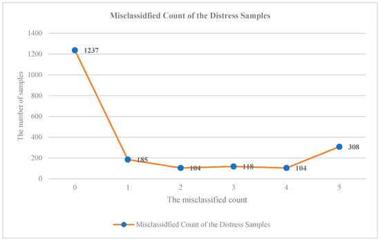
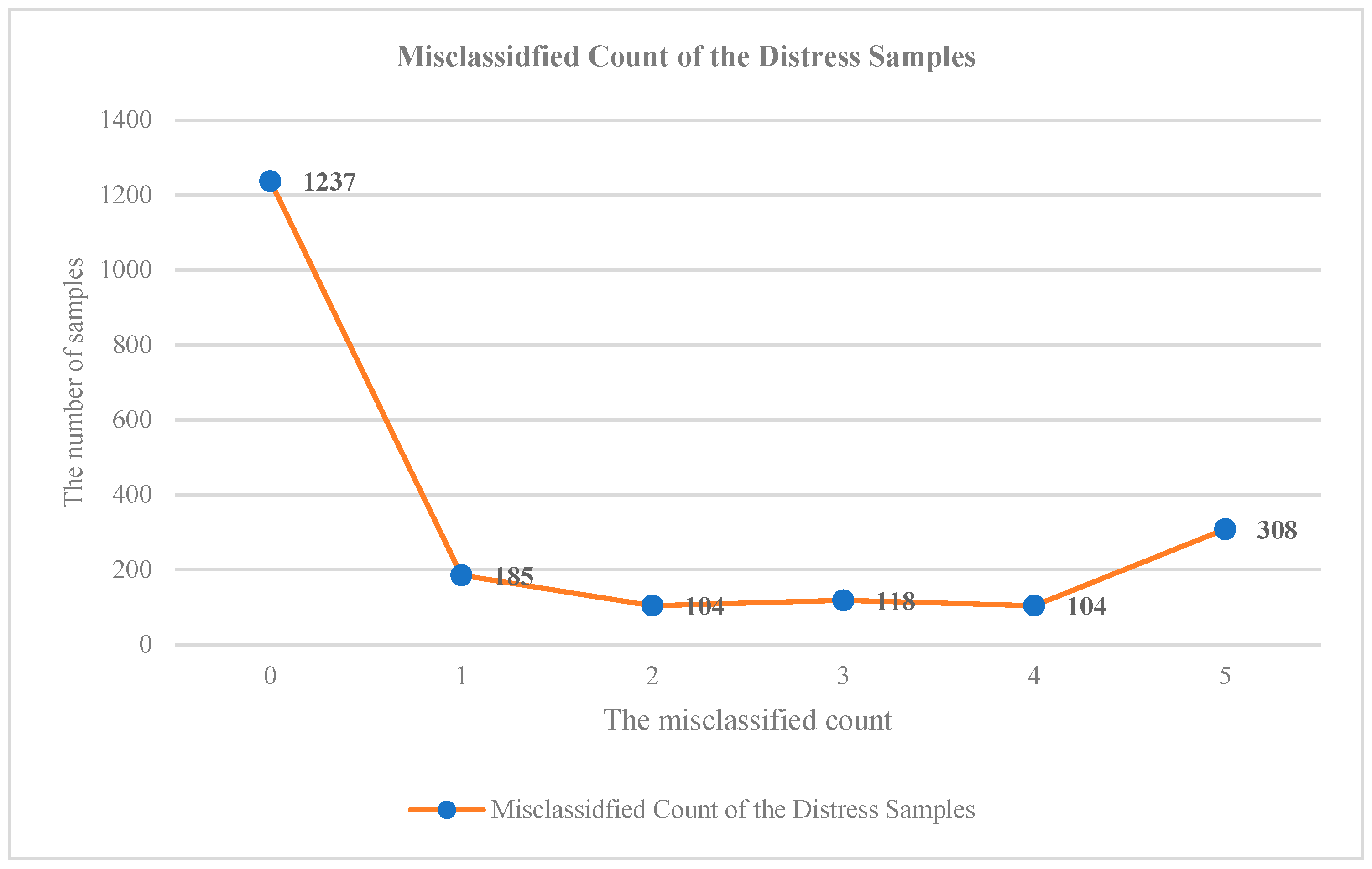
Figure 9 reveals critical insights into how distress samples are repeatedly misclassified in DWARFB model training process. Amongst 2056 distress samples, 1237 (60%) were consistently classified correctly across all training iterations, suggesting that the DWARFB model effectively learned the underlying patterns of these samples. However, 308 (15%) samples were cumulatively misclassified five times, suggesting that these are particularly challenging cases, and that retaining misclassification information from the previous five training iterations is still insufficient for the DWARFB model to effectively capture their underlying patterns. 514 (25%) samples that were persistently misclassified four times or fewer appear to have had their “hardness” patterns successfully learned by the model.

Figure 9. The misclassified count of the distress samples in the training process.

Approximately 85% of the distress samples were correctly learned by the DWARFB model, indicating that the misclassification enhancement mechanism effectively adjusts sample weights based on the distress samples’ pattern recognition. The process also rewards samples that are consistently predicted correctly for two consecutive training rounds. This adaptive weighting strategy strengthens the model’s focus on informative samples and enhances classification stability throughout the iterative learning process.

The DWARFB model was configured to retain misclassification information from the five most recent training iterations to prevent cumulative excessive weighting of misclassified samples. However, some samples are still repeatedly misclassified across five or more iterations. Removing this retention threshold could lead to excessive weight being assigned to misclassified samples. This imbalance may distort the model’s behavior, granting undue influence on difficult samples or even weakening the effectiveness of the penalty mechanism. Therefore, careful balancing between enhanced weighting and preventing error accumulation is essential to identify underlying causes and guide future model refinement.

4.7. Loss-Based Feature Contributions

The loss-based contribution serves as a performance-driven metric of feature importance, evaluating how much each feature reduces classification loss during DWARFB training. Table 6 illustrates the top 20 features ranked by their loss-based contributions.

Table 6. The top 20 feature contributions.

Rank	Feature	Description	Contribution
1	Var318	Undistributed Profit per Share	0.040
2	Var61	Ratio of Retained Earnings to Total Assets	0.030
3	Var313	Net Assets per Share	0.028
4	Var319	Retained Earnings per Share	0.025
5	Var320	Net Assets per Share Attributable to the Parent Company	0.018
6	Q2_Var319	Q2_Retained Earnings per Share	0.016
7	Var17	Earnings Volatility	0.015
8	Q2_Var61	Q2_Ratio of Retained Earnings to Total Assets	0.012
9	Q2_Var318	Q2_Undistributed Profit per Share	0.010
10	Var324	Net Cash Flow from Investing Activities per Share—TTM	0.010
11	Q2_Var312	Q2_Operating Profit per Share—TTM	0.010
12	Q2_Var320	Q2_Net Assets per Share Attributable to the Parent Company	0.009
13	Q2_Var47	Q2_Basic Earnings per Share after Deducting Extraordinary Items	0.009
14	Q2_Var313	Q2_Net Assets per Share	0.009
15	Var323	Net Cash Flow from Investing Activities per Share	0.009
16	Q2_Var292	Q2_Earnings per Share—TTM3	0.009
17	Var348	Price to Earnings Attributable to the Parent Company	0.009
18	Var314	Tangible Assets per Share	0.009
19	Var47	Basic Earnings per Share after Deducting Extraordinary Items	0.009
20	Q2_Var294	Q2_Earnings per Share—TTM4	0.008

To facilitate economic interpretation, these features are grouped into five categories according to their financial meaning.

Category 1 Retained earnings and accumulated profitability: This group comprises six highly related indicators, including Undistributed Profit per Share (Var318, Q2_Var318), Ratio of Retained Earnings to Total Assets (Var61, Q2_Var61), and Retained Earnings per Share (Var319, Q2_Var319). These variables dominate the ranking, 6 out of the top 9 positions, with Var318 exhibiting the highest contribution (0.040) among all features. This indicates that cumulative profitability and internal capital accumulation capacity play a decisive role in reducing misclassification loss in DWARFB.

In conventional financial distress theory, retained earnings reflect a firm’s long-term ability to generate profits and build financial buffers against adverse shocks. Firms that fail to retain or accumulate profits are therefore more vulnerable to financial distress. This finding is highly consistent with traditional bankruptcy prediction models, such as Altman Z-score, the X2 indicator (Retained Earnings/Total Assets), in which retained earnings-related ratios are core explanatory variables [34,35].

Category 2 Equity strength and asset backing: Five highly associated indicators are Net Assets per Share (Var313, Q2_Var313), Net Assets per Share Attributable to the Parent Company (Var320, Q2_Var320), and Tangible Assets per Share (Var314).

These features measure the extent to which shareholders’ equity and tangible assets support the firm’s operations. Their relatively high contributions suggest that balance-sheet solidity plays a key role in correcting classification errors. Equity and tangible assets represent the fundamental solvency of a firm. A stronger equity base implies a greater capacity to absorb losses and sustain operations, whereas erosion of net assets is often a precursor to financial distress [36].

Category 3 Current profitability and earnings quality: This category includes Operating Profit per Share (Q2_Var312), Basic Earnings per Share after Deducting Extraordinary Items (Var47, Q2_Var47), and Earnings per Share (Q2_Var292, and Q2_Var294), which capture short-term operational performance and sustainable earning power. Their moderate contributions in DWARFB suggest that contemporaneous profitability helps refine predictions but is secondary to accumulated profitability and equity strength. Financially, this reflects the idea that temporary profits or losses are informative, but long-term financial structure is more decisive in determining distress risk [37].

Category 4 Earnings stability: One indicator (Earnings Volatility, Var17) is identified. Unlike level-based profitability measures, this variable captures the risk dimension of firm performance. Its relatively high ranking (rank 7th, 0.015) implies that firms with unstable earnings are more prone to distress, which is consistent with prior studies showing that earnings volatility significantly increases distress probability [38].

Category 5 Cash flow and market valuation signals: Three variables were identified in this category. These variables include Net Cash Flow from Investing Activities per Share (Var324, Var323) and Price-to-Earnings Attributable to the Parent Company (Var348). In the training process, these features play a complementary role, contributing to loss reduction but to a lesser extent than accounting-based fundamentals.

Overall, the categorical structure of the top contributing features reveals a clear hierarchy in DWARFB: accumulated profitability and retained earnings dominate, followed by equity strength, current profitability, earnings stability, and finally cash flow and market-based signals. Many of these top features are lagged indicators (Q2), highlighting that incorporating lagged features can provide early warning signals and shape the predictive hierarchy. This hierarchy closely mirrors the financial logic underlying classical distress prediction models, while the proposed loss-based contribution metric further enhances interpretability by directly linking feature importance to reductions in misclassification loss during training.

4.8. Summary of Findings

This study identifies three major gaps in current financial distress prediction methods. These include rigid iterative training, static sample enhancement, and inflexible ensemble combination. The findings indicate that the DWARFB model effectively resolves all three challenges.

First, unlike conventional boosting algorithms with fixed weight-adjustment rules, DWARFB applies adaptive misclassification weighting. It captures cumulative misclassification patterns and dynamically emphasizes persistently difficult samples. This design prevents error accumulation and improves learning from structurally complex cases. As a result, the limitations of rigid iterative training have been effectively resolved.

Second, by addressing the static treatment of difficult samples in traditional resampling approaches, DWARFB continuously updates sample importance based on their evolving classification behavior. Consequently, about 85% of distress samples are correctly classified across iterations (with 60% consistently classified correctly in all rounds), leaving only a small fraction of 15% persistently hard-to-learn cases. At the same time, the loss-based feature contribution metric demonstrates strong economic interpretability: it naturally rediscovers the core financial logic underlying classical distress prediction models, such as the dominance of retained earnings, accumulated profitability, and equity strength, while further enhancing it through a dynamic, misclassification-aware learning mechanism.

Third, DWARFB enhances ensemble flexibility by using an adaptive weighting strategy that responds to performance dynamics across iterations. This approach produces a more balanced trade-off between precision and recall. Empirical evaluations show that DWARFB delivers strong and stable predictive performance (F1-score = 0.62 ± 0.01, MCC = 0.60 ± 0.01, PR-AUC = 0.662), surpassing standard, cost-sensitive, and resampling-based random forest baselines.

The hyperparameter analysis shows that deeper trees with smaller leaves and a moderate ensemble size best balance accuracy and efficiency in DWARFB.

Overall, DWARFB successfully bridges the identified methodological gaps through its adaptive, cumulative misclassification awareness and flexible learning design, establishing a robust and reliable framework for early financial distress prediction.

5. Conclusions

This study addresses three critical limitations in existing financial distress prediction models, which are rigidity in handling class imbalance, static treatment of persistently misclassified samples, and inflexible ensemble combination strategies. To alleviate these limitations, we propose a novel framework named Dynamic Weight-Adjusted Random Forest Boost (DWARFB). DWARFB integrates three core innovations: dynamic sample weighting scheme, dynamic class ratios, and real-time model weight adjustment.

The performance of DWARFB was examined using the financial data from 1174 Chinese-listed companies sourced from the CSMAR database. The dataset contains 52,528 samples with 368 features, categorized into two classes: 2973 distressed and 49,555 normal samples.

Comparative analyses against eight baseline Random Forest (RF) methods demonstrated that DWARFB achieves superior balanced performance. It outperforms all baselines with the highest F1-score (0.62 ± 0.01), MCC (0.60 ± 0.01), ROC-AUC (0.954), and PR-AUC (0.662). Notably, while under-sampling methods (e.g., RF + RUS) yield high recall (0.89), they suffer from drastically reduced precision (~0.30). Standard RF exhibits high precision (0.75) but low recall (0.38). In contrast, DWARFB maintains a robust trade-off between precision (0.58 ± 0.04) and recall (0.67 ± 0.05), a critical advantage for high-stakes financial risk management.

Statistical analysis on pairwise Wilcoxon signed-rank tests across 20 independent runs confirmed that DWARFB’s performance gains are consistent and statistically significant (p-value < 0.001 in all experiments). Large Cohen’s effect size (d = 8.63–42.47) further supports these findings.

In terms of hyperparameter tuning on the RF learner, we found that a maximum tree depth of 15 and a minimum sample per leaf of 1 are the most influential settings for predictive power. To achieve a practical balance between accuracy and computational efficiency, it is recommended to construct at least 50 decision trees before aggregating prediction results.

The effective integration of dynamic sample reweighting and loss-based feature contributions enhances both the detection of hard-to-classify samples and the interpretability of DWARFB.

The primary limitation of DWARFB lies in its longer training time (387.9 s) when compared to baselines, which may constrain deployment in time-sensitive scenarios. However, this trade-off is justified by its enhanced predictive reliability, a priority in financial distress prediction, where missed detections of distressed firms can lead to severe economic losses or regulatory penalties.

Future research directions include: (1) improving computational efficiency via parallelized or distributed training and adaptive early stopping; (2) enhancing adaptability to extreme class imbalance by exploring a wider range of sampling ratios and dynamic adjustment strategies; (3) validating DWARFB on cross-country financial datasets to assess its generalizability beyond Chinese listed companies; and (4) the trade-off between enhanced misclassified punishment and preventing error accumulation to identify underlying causes and guide future model refinement in the misclassified enhancement mechanism.

In summary, DWARFB provides a more adaptive, robust, and practically valuable tool for early financial distress warning systems. By dynamically weighting persistently hard-to-classify samples, it effectively addresses the limitations of static sample weighting in traditional resampling and weighted approaches. This mechanism enables high classification accuracy for most distressed samples, thereby advancing the state of the art in imbalanced and dynamic financial distress prediction.

References

- Abdelkader, N.A.M.; Wahba, H.H. A Proposed Multidimensional Model for Predicting Financial Distress: An Empirical Study on Egyptian Listed Firms. Future Bus. J. 2024, 10, 42. [Google Scholar] [CrossRef] [Scilit]
- Nguyen, H.H.; Viviani, J.-L.; Ben Jabeur, S. Bankruptcy Prediction Using Machine Learning and Shapley Additive Explanations. Rev. Quant. Financ. Account. 2025, 65, 107–148. [Google Scholar] [CrossRef] [Scilit]
- Hajek, P.; Munk, M. Speech Emotion Recognition and Text Sentiment Analysis for Financial Distress Prediction. Neural Comput. Applic 2023, 35, 21463–21477. [Google Scholar] [CrossRef] [Scilit]
- Imani, M.; Beikmohammadi, A.; Arabnia, H.R. Comprehensive Analysis of Random Forest and XGBoost Performance with SMOTE, ADASYN, and GNUS under Varying Imbalance Levels. Technologies 2025, 13, 88. [Google Scholar] [CrossRef] [Scilit]
- Dube, L.; Verster, T. Enhancing Classification Performance in Imbalanced Datasets: A Comparative Analysis of Machine Learning Models. Data Sci. Financ. Econ. 2023, 3, 354–379. [Google Scholar] [CrossRef] [Scilit]
- Ding, Y.; Zhu, H.; Chen, R.; Li, R. An Efficient AdaBoost Algorithm with the Multiple Thresholds Classification. Appl. Sci. 2022, 12, 5872. [Google Scholar] [CrossRef] [Scilit]
- Sermpinis, G.; Tsoukas, S.; Zhang, Y. Modelling Failure Rates with Machine-learning Models: Evidence from a Panel of UK Firms. Euro Fin. Manag. 2023, 29, 734–763. [Google Scholar] [CrossRef] [Scilit]
- Sibindi, R.; Mwangi, R.W.; Waititu, A.G. A Boosting Ensemble Learning Based Hybrid Light Gradient Boosting Machine and Extreme Gradient Boosting Model for Predicting House Prices. Eng. Rep. 2023, 5, e12599. [Google Scholar] [CrossRef] [Scilit]
- Walmsley, F.N.; Cavalcanti, G.D.C.; Oliveira, D.V.R.; Cruz, R.M.O.; Sabourin, R. An Ensemble Generation Method Based on Instance Hardness. In Proceedings of the 2018 International Joint Conference on Neural Networks (IJCNN), Rio de Janeiro, Brazil, 8–13 July 2018; pp. 1–8. [Google Scholar] [CrossRef] [Scilit]
- Shen, F.; Liu, Y.; Wang, R.; Zhou, W. A Dynamic Financial Distress Forecast Model with Multiple Forecast Results under Unbalanced Data Environment. Knowl.-Based Syst. 2020, 192, 105365. [Google Scholar] [CrossRef] [Scilit]
- Lin, J.C.-W.; Gan, W.; Fournier-Viger, P.; Hong, T.-P.; Zhan, J. Efficient Mining of High-Utility Itemsets Using Multiple Minimum Utility Thresholds. Knowl.-Based Syst. 2016, 113, 100–115. [Google Scholar] [CrossRef] [Scilit]
- Hou, G.; Tong, D.L.; Liew, S.Y.; Choo, P.Y. Comparative Analysis of Resampling Techniques for Class Imbalance in Financial Distress Prediction Using XGBoost. Mathematics 2025, 13, 2186. [Google Scholar] [CrossRef] [Scilit]
- Kadkhoda, S.T.; Amiri, B. A Hybrid Network Analysis and Machine Learning Model for Enhanced Financial Distress Prediction. IEEE Access 2024, 12, 52759–52777. [Google Scholar] [CrossRef] [Scilit]
- Le, T. A Comprehensive Survey of Imbalanced Learning Methods for Bankruptcy Prediction. IET Commun. 2022, 16, 433–441. [Google Scholar] [CrossRef] [Scilit]
- Ramakrishna, M.T.; Venkatesan, V.K.; Izonin, I.; Havryliuk, M.; Bhat, C.R. Homogeneous Adaboost Ensemble Machine Learning Algorithms with Reduced Entropy on Balanced Data. Entropy 2023, 25, 245. [Google Scholar] [CrossRef] [Scilit]
- Sun, J.; Jia, M.; Li, H. AdaBoost Ensemble for Financial Distress Prediction: An Empirical Comparison with Data from Chinese Listed Companies. Expert. Syst. Appl. 2011, 38, 9305–9312. [Google Scholar] [CrossRef] [Scilit]
- Friedman, J.H. Greedy Function Approximation: A Gradient Boosting Machine. Ann. Statist. 2001, 29, 1189–1232. [Google Scholar] [CrossRef] [Scilit]
- Huang, W.-C. Integrating Gaussian Processes and Adaptive Boosting for Complex Time Series Forecasting of S&P 500 Index. Contemp. Math. 2025, 6, 3670–3685. [Google Scholar] [CrossRef] [Scilit]
- De Bock, K.W.; Coussement, K.; Lessmann, S. Cost-Sensitive Business Failure Prediction When Misclassification Costs Are Uncertain: A Heterogeneous Ensemble Selection Approach. Eur. J. Oper. Res. 2020, 285, 612–630. [Google Scholar] [CrossRef] [Scilit]
- Tanha, J.; Abdi, Y.; Samadi, N.; Razzaghi, N.; Asadpour, M. Boosting Methods for Multi-Class Imbalanced Data Classification: An Experimental Review. J. Big Data 2020, 7, 70. [Google Scholar] [CrossRef] [Scilit]
- Yi, Z. Credit Default Risk Measurement and Statistical Analysis Based on Improved GRU Model. Eng. Rep. 2025, 7, e70014. [Google Scholar] [CrossRef] [Scilit]
- Wang, J.-B.; Zou, C.-A.; Fu, G.-H. AWSMOTE: An SVM-Based Adaptive Weighted SMOTE for Class-Imbalance Learning. Sci. Program. 2021, 2021, 9947621. [Google Scholar] [CrossRef] [Scilit]
- Vasheghani, S.; Sharifi, S. Adaptive Dynamic Ensemble Learning with Class-Specific Model Selection for Efficient and Robust Image Classification. Knowl.-Based Syst. 2025, 331, 114842. [Google Scholar] [CrossRef] [Scilit]
- Gnip, P.; Kanász, R.; Zoričak, M.; Drotár, P. An Experimental Survey of Imbalanced Learning Algorithms for Bankruptcy Prediction. Artif. Intell. Rev. 2025, 58, 104. [Google Scholar] [CrossRef] [Scilit]
- Malek, N.H.A.; Yaacob, W.F.W.; Wah, Y.B.; Md Nasir, S.A.; Shaadan, N.; Indratno, S.W. Comparison of Ensemble Hybrid Sampling with Bagging and Boosting Machine Learning Approach for Imbalanced Data. Indones. J. Electr. Eng. Comput. Sci. 2022, 29, 598. [Google Scholar] [CrossRef] [Scilit]
- Aljawazneh, H.; Mora, A.M.; Garcia-Sanchez, P.; Castillo-Valdivieso, P.A. Comparing the Performance of Deep Learning Methods to Predict Companies’ Financial Failure. IEEE Access 2021, 9, 97010–97038. [Google Scholar] [CrossRef] [Scilit]
- Aljawazneh, H.; Yaseen, S.G.; Al-Shayea, Q. Bagging vs Boosting Ensemble Classifiers in Predicting Companies’ Financial Status. In Cutting-Edge Business Technologies in the Big Data Era; Yaseen, S.G., Ed.; Studies in Big Data; Springer Nature: Cham, Switzerland, 2023; Volume 135, pp. 1–9. ISBN 978-3-031-42465-6. [Google Scholar] [CrossRef] [Scilit]
- Winsor, C.P. The Gompertz Curve as a Growth Curve. Proc. Natl. Acad. Sci. USA 1932, 18, 1–8. [Google Scholar] [CrossRef] [Scilit]
- Freund, Y.; Schapire, R.E. A Decision-Theoretic Generalization of On-Line Learning and an Application to Boosting. J. Comput. Syst. Sci. 1997, 55, 119–139. [Google Scholar] [CrossRef] [Scilit]
- Lin, T.-Y.; Goyal, P.; Girshick, R.; He, K.; Dollar, P. Focal Loss for Dense Object Detection. In Proceedings of the 2017 IEEE International Conference on Computer Vision (ICCV), Venice, Italy, 22–29 October 2017; pp. 2999–3007. [Google Scholar] [CrossRef] [Scilit]
- Shrivastava, A.; Gupta, A.; Girshick, R. Training Region-Based Object Detectors with Online Hard Example Mining. In Proceedings of the 2016 IEEE Conference on Computer Vision and Pattern Recognition (CVPR), Las Vegas, NV, USA, 27–30 June 2016; pp. 761–769. [Google Scholar] [CrossRef] [Scilit]
- Fleiss, J.L.; Cohen, J. The Equivalence of Weighted Kappa and the Intraclass Correlation Coefficient as Measures of Reliability. Educ. Psychol. Meas. 1973, 33, 613–619. [Google Scholar] [CrossRef] [Scilit]
- Rey, D.; Neuhäuser, M. Wilcoxon-Signed-Rank Test. In International Encyclopedia of Statistical Science; Lovric, M., Ed.; Springer: Berlin, Heidelberg, 2011; pp. 1658–1659. ISBN 978-3-642-04897-5. [Google Scholar] [CrossRef] [Scilit]
- Sánchez-Almeyda, C.; González-Bueno, J.; Koval, V.; Reyes-Maldonado, N.; Kryshtal, H.; Zharikova, O. Predicting Financial Distress in the Food Production Sector: A Dual-Model Approach Using Z-Score and O-Score Methods. Discov. Sustain. 2025, 6, 731. [Google Scholar] [CrossRef] [Scilit]
- Santoso, N.W.; Kusumawardhani, R.; Maulida, A. Comparative Analysis of the Altman, Ohlson, and Zmijewski Models to Predict Financial Distress during the Covid-19 Pandemic. MAKSIMUM 2024, 14, 13. [Google Scholar] [CrossRef] [Scilit]
- Modina, M.; Zedda, S. Diagnosing Default Syndromes: Early Symptoms of Entrepreneurial Venture Insolvency. J. Small Bus. Enterp. Dev. 2023, 30, 186–209. [Google Scholar] [CrossRef] [Scilit]
- Mavengere, K.; Gumede, P. Financial Distress Prediction Competence of the Altman Z Score and Zmijewski Model: Evidence from Selected Zimbabwe Stock Exchange Firms. Pressacademia 2024, 11, 9–15. [Google Scholar] [CrossRef] [Scilit]
- Saadaoui, Z.; Mokdadi, S. Capital Buffers, Business Models and the Probability of Bank Distress: A Dynamic Panel Investigation. J. Financ. Regul. Compliance 2023, 31, 663–695. [Google Scholar] [CrossRef] [Scilit]
Disclaimer/Publisher’s Note: The statements, opinions and data contained in all publications are solely those of the individual author(s) and contributor(s) and not of MDPI and/or the editor(s). MDPI and/or the editor(s) disclaim responsibility for any injury to people or property resulting from any ideas, methods, instructions or products referred to in the content. |
© 2026 by the authors. Licensee MDPI, Basel, Switzerland. This article is an open access article distributed under the terms and conditions of the Creative Commons Attribution (CC BY) license.