Threshold Dynamics of a SIRI Model with Reinfection: Averaged and Periodic Systems and Application to Tuberculosis Data

Abstract

Tuberculosis (TB) remains a major public health challenge in high-burden regions, where reinfection and seasonal variation play important roles in disease transmission. In this paper, we study a tuberculosis transmission model with reinfection based on the SIRI framework, with particular emphasis on the intrinsic relationship between the averaged system and the periodic system. The averaged system is shown to characterize the long-term epidemiological behavior, whereas the periodic system captures short-term seasonal fluctuations. From a theoretical perspective, we prove that the periodic system and its corresponding averaged system share the same basic reproduction number. We analyze the threshold dynamics of the seasonal model and investigate the dynamical properties of the averaged system, including the existence and stability of equilibria and the occurrence of backward bifurcation. In particular, we show that disease persistence may occur even when the basic reproduction number ($R_0$) is less than one, and we examine the stability of equilibrium points at the critical threshold ($R_0=1$). These results reveal how transmission and reinfection jointly determine the disease burden and equilibrium structure. To validate the theoretical findings, numerical simulations are performed using tuberculosis incidence data from Yunnan Province, China, covering the period from 2005 to 2020. The numerical simulations suggest that the seasonal model provides a better fit to the data, while the averaged model may overestimate the transmission potential of the disease. Under the condition that the two models share the same basic reproduction number, a constrained numerical simulation is performed. The results show that, under certain parameter settings, the endemic equilibrium of the averaged system can approximate the mean prevalence of the periodic solution. However, such an approximation cannot be guaranteed in general.

1. Introduction

Infectious diseases caused by pathogenic microorganisms or parasites spread among living hosts and continue to pose major challenges to global public health. Tuberculosis (TB) is a chronic and highly contagious disease caused by Mycobacterium tuberculosis. It is one of the most serious infectious diseases in the world. Despite long-term control measures, tuberculosis remains difficult to eliminate due to its complex transmission mechanism, long infectious period and the possibility of reinfection after recovery. Mathematical modeling has become an important tool for understanding the dynamics of tuberculosis transmission and evaluating intervention strategies.

The classic SIR Model proposed by Kermack and McKendrick [1,2,3] classified the population into susceptible, infected and recovered groups, laying a theoretical foundation for epidemic modeling. However, this framework is insufficient for diseases such as tuberculosis, as only partial immunity is acquired after recovery. People who have recovered from tuberculosis are still prone to reinfection. To better capture this epidemiological reality, researchers extended the classical model to the SIRI framework [4,5,6], incorporating a mechanism that enables recovered individuals to return to the infected class. Recurrence of tuberculosis involves two main pathways: endogenous reactivation of latent bacteria and exogenous reinfection caused by re-exposure to the pathogen [7]. In low TB burden settings, recurrences were mainly caused by relapse [8]. In high TB burden settings, molecular epidemiological studies have demonstrated that recurrent tuberculosis cases are predominantly caused by exogenous reinfection rather than relapse of the original infection [9]. Reinfection is more likely in high-burden regions than in low-burden regions [10,11]. Research on the relative roles of relapse and reinfection in tuberculosis recurrence is still ongoing [12]. Most early tuberculosis models assumed that the transmission rate and reinfection rate remained constant, thus forming autonomous systems. However, empirical epidemiological data indicate that the incidence of tuberculosis often shows temporal variations due to factors such as seasonal climate change, social behavior, access to healthcare, and policy intervention. Epidemiological data of tuberculosis (TB) cases show seasonal fluctuations in many countries [13,14,15,16,17]. Kirolos et al. [18] reported that tuberculosis case notification rates (CNRs) in Blantyre show a clear seasonal pattern with two annual peaks, coinciding with the start and end of the rainy season. Taylan et al. [19] investigate seasonal variability by statistical curve fitting, surface fitting, and autoregressive time series analysis. Xue et al. [20] developed an age-structured tuberculosis transmission model with seasonal transmission and evaluated vaccination, diagnostic, and treatment strategies, as well as their combinations, for achieving the WHO targets in China. Liu et al. [21] developed a seasonal tuberculosis model to investigate the seasonal patterns of newly reported tuberculosis cases in the mainland of China. To capture these features, the periodic transmission rate has been widely incorporated into tuberculosis models, thereby forming a seasonal system [22,23]. Previous studies have shown that pulmonary tuberculosis in Yunnan Province, as a high-burden setting [24], exhibits pronounced seasonal patterns [25,26], while reinfection remains a non-negligible feature.

Based on the SIRI framework proposed in [27], we construct a seasonal tuberculosis transmission model with periodically varying transmission and reinfection rates. By taking temporal averages of the periodic coefficients, the corresponding averaged system is derived. The aim of this study is to explore the intrinsic relationship between the principal dynamical features of periodic epidemic systems and those of their corresponding averaged systems. We analyze the basic reproduction numbers of both the periodic system and the averaged system, and show that they share the same basic reproduction number. Moreover, the threshold dynamics of the seasonal tuberculosis model are investigated. For the averaged system, we conduct a detailed analysis of its stability and bifurcation behavior, with particular emphasis on the stability of equilibria at the critical threshold $R_0=1$. Numerical simulations based on tuberculosis data from Yunnan Province are performed to illustrate and validate the theoretical results.

The remainder of this paper is organized as follows. In Section 2, we formulate the seasonal tuberculosis model and analyze its basic reproduction number and threshold dynamics. In Section 3, we derive the corresponding averaged system and investigate its stability and bifurcation properties, with special attention given to the case $R_0=1$. Section 4 presents numerical simulations to illustrate the theoretical results. Finally, conclusions is given in Section 5.

2. The Seasonal TB Model

In this section, motivated by the observed seasonality in newly reported TB cases in Yunnan Province and the role of reinfection, we consider a model with $\omega$-periodic coefficients to reflect seasonal forcing.

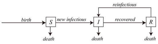
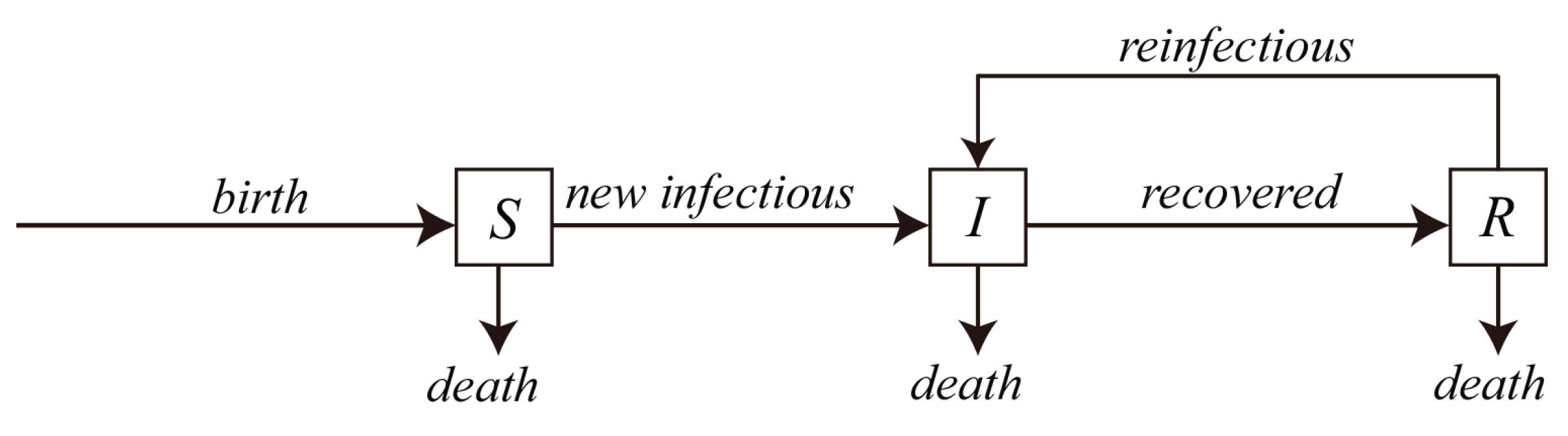
From a biological point of view, we consider a disease transmission mechanism incorporating population mobility, including population inflow and outflow, as well as transitions of individuals among three epidemiological categories. Based on this mechanism, a transmission model is constructed by incorporating infection, recovery, reinfection, and migration processes. The main aim of this paper is to reveal a simple and biologically sound mechanism that explains the input–output dynamics of disease transmission. We assume that TB spreads in a population of size $N\left(t\right)$, where $N\left(t\right)$ denotes the total population size. $S\left(t\right)$, $I\left(t\right)$, and $R\left(t\right)$ represent the numbers of susceptible, infectious, and recovered individuals at time t, respectively. The transmission process diagram with population input and output is shown in Figure 1. In the schematic diagram, arrows represent the movement of individuals between compartments.

Figure 1. Schematic diagram for the TB transmission model with reinfection.

During the spread of a disease with reinfection, the goal of modeling is to track the number of individuals in each of the three compartments at any given time t. Considering reinfection, we model TB transmission within an input–output framework, where selected coefficients are assumed to be periodic functions of time, reflecting the seasonal trend commonly observed in TB incidence data.

The force of infection at time t is given by $\overline{\beta }\left(t\right)I\left(t\right)$, where $\overline{\beta }\left(t\right)$ is an $\omega$-periodic transmission rate for some $\omega >0$. Similarly, the force of reinfection at time t is given by $\overline{\lambda }\left(t\right)I\left(t\right)$, where $\overline{\lambda }\left(t\right)$ is an $\omega$-periodic reinfection rate for some $\omega >0$. The parameter $\alpha$ denotes the recovery rate, representing the proportion of infected individuals who recover per unit time. Its reciprocal ${\displaystyle \frac{1}{\alpha }}$ indicates the average duration of infection. We further consider birth–death (or inflow–outflow) processes in the population. To simplify the model, we assume that the per capita birth rate is equal to the per capita death rate, both denoted by b. All model parameters are assumed to be positive and biologically feasible.

Based on the above assumptions, we obtain the following system of non-autonomous differential equations:

$$\left\{\begin{array}{cc}\hfill \dot{S}\left(t\right)& =bN\left(t\right)-\overline{\beta }\left(t\right)I\left(t\right)S\left(t\right)-bS\left(t\right),\hfill \\ \hfill \dot{I}\left(t\right)& =\overline{\beta }\left(t\right)I\left(t\right)S\left(t\right)+\overline{\lambda }\left(t\right)I\left(t\right)R\left(t\right)-\alpha I\left(t\right)-bI\left(t\right),\hfill \\ \hfill \dot{R}\left(t\right)& =\alpha I\left(t\right)-\overline{\lambda }\left(t\right)I\left(t\right)R\left(t\right)-bR\left(t\right),\hfill \end{array}\right.$$

(1)

with initial conditions $S\left(0\right)\ge 0$, $I\left(0\right)\ge 0$, $R\left(0\right)\ge 0$.

System (1) describes the transitions of individuals among different compartments, and illustrates the effects of interventions and seasonal fluctuations on disease transmission through the periodic coefficients $\overline{\beta }\left(t\right)$ and $\overline{\lambda }\left(t\right)$. By summing all three equations in System (1), we obtain $\dot{N}\left(t\right)=0$, which implies that $N\left(t\right)=K$ is constant for all $t\ge 0$, where $K=S\left(0\right)+I\left(0\right)+R\left(0\right)$. In the subsequent analysis, the total population size $N\left(t\right)$ is replaced by the constant K. Consequently, the non-autonomous periodic epidemic Model (1) can be rewritten in the following equivalent form:

$$\left\{\begin{array}{cc}\hfill \dot{S}\left(t\right)& =bK-\overline{\beta }\left(t\right)I\left(t\right)S\left(t\right)-bS\left(t\right),\hfill \\ \hfill \dot{I}\left(t\right)& =\overline{\beta }\left(t\right)I\left(t\right)S\left(t\right)+\overline{\lambda }\left(t\right)I\left(t\right)R\left(t\right)-\alpha I\left(t\right)-bI\left(t\right),\hfill \\ \hfill \dot{R}\left(t\right)& =\alpha I\left(t\right)-\overline{\lambda }\left(t\right)I\left(t\right)R\left(t\right)-bR\left(t\right).\hfill \end{array}\right.$$

(2)

2.1. The Basic Reproduction Number

Setting $I\left(t\right)=0$, System (2) admits the disease-free equilibrium $Q_0=(K,0,0)$. Linearizing the infected equation of System (2) at the disease-free equilibrium, we obtain

$$\dot{I}\left(t\right)=(\overline{\beta }\left(t\right)K-(\alpha +b))I\left(t\right),$$

(3)

which is a scalar linear periodic equation.

Now, we introduce

$$F\left(t\right)=\overline{\beta }\left(t\right)K,V\left(t\right)=\alpha +b.$$

Following the framework of Wang and Zhao [28], we adopt the following setting. Let ${\mathsf{\Phi }}_{-V}\left(t\right)$ be the monodromy matrix of the linear $\omega$-periodic system ${\displaystyle \frac{dz}{dt}}=-V\left(t\right)z$. Assume that $Y(t,s)$, $t⩾s$, is the evolution operator of the linear $\omega$-periodic system

$${\displaystyle \frac{dy}{dt}}=-V\left(t\right)y.$$

(4)

That is, for each $s\in \mathbb{R}$, $Y(t,s)$ satisfies

$${\displaystyle \frac{d}{dt}}Y(t,s)=-V\left(t\right)Y(t,s),\forall t\ge s,Y(s,s)=1.$$

Thus, the monodromy matrix ${\mathsf{\Phi }}_{-V}\left(t\right)$ of (4) is equal to $Y(t,0),t\ge 0$.

In view of the periodic environment, we assume that $\psi \left(s\right)$, $\omega$-periodic in s, is the initial distribution of infectious individuals. Then, $F\left(s\right)\psi \left(s\right)$ is the rate of new infections produced by the infected individuals who were introduced at time s. Given $t\ge s$, then $Y(t,s)F\left(s\right)\psi \left(s\right)$ gives the distribution of those infected individuals who were newly infected at time s and remain in the infected compartments at time t. It follows that

$$\begin{array}{cc}\hfill \psi \left(t\right)& ={\int }_{-\infty }^{t}Y(t,s)F\left(s\right)\psi \left(s\right)ds={\int }_0^{\infty }Y(t,t-a)F(t-a)\psi (t-a)da\hfill \end{array}$$

is the distribution of accumulative new infections at time t produced by all those infected individuals $\psi \left(s\right)$ introduced at time previous to t.

Let $C_{\omega }$ be the ordered Banach space of all $\omega$-periodic functions from $\mathbb{R}$ to $\mathbb{R}$, equipped with the maximum norm $\parallel ·\parallel$, and let the positive cone be

$$C_{\omega }^{+}=\left\{\varphi \in C_{\omega }\mid \varphi \left(t\right)\ge 0,\forall t\in \mathbb{R}\right\}.$$

Then we can define a linear operator $L:C_{\omega }\to C_{\omega }$ by

$$\left(L\varphi \right)\left(t\right)={\int }_0^{\infty }Y(t,t-a)F(t-a)\varphi (t-a)da,\forall t\in \mathbb{R},\varphi \in C_{\omega }.$$

The basic reproduction number of System (2) is then defined as

$${\mathcal{R}}_0:=\rho \left(L\right),$$

(5)

where $\rho \left(L\right)$ denotes the spectral radius of L.

Since $V\left(t\right)\equiv \alpha +b$ is a constant, we obtain $Y(t,s)=e^{-(\alpha +b)(t-s)}$ which greatly simplifies the analysis. Furthermore, we can give the explicit expression of the basic reproduction number ${\mathcal{R}}_0$. Let $W(t,s,\xi )$, $t\ge s$, be the evolution operator of the linear periodic system

$$\dot{w}\left(t\right)=[-V\left(t\right)+{\displaystyle \frac{F\left(t\right)}{\xi }}]w\left(t\right)$$

with parameter $\xi$. Hence

$$w\left(t\right)=W(t,s,\xi )w\left(s\right).$$

Denote $a\left(t\right)=-V\left(t\right)+{\displaystyle \frac{F\left(t\right)}{\xi }}$. For the scalar equation

$$\dot{w}\left(t\right)=a\left(t\right)w\left(t\right),$$

its solution is given exactly by

$$w\left(t\right)=w\left(s\right)exp\left({\int }_s^{t}a\left(\tau \right)d\tau \right).$$

Therefore, the evolution operator can be written as

$$W(t,s,\xi )=exp\left({\int }_s^t\left[-V\left(\tau \right)+{\displaystyle \frac{F\left(\tau \right)}{\xi }}\right]d\tau \right)=exp\left({\int }_s^t\left[-(\alpha +b)+{\displaystyle \frac{\overline{\beta }\left(\tau \right)K}{\xi }}\right]d\tau \right).$$

Applying the results in [28] (see Theorem 2.1), the following statements hold:

(1) If $\rho \left(W(\omega ,0,\xi )\right)=1$ has a positive solution ${\xi }_0$, then ${\xi }_0$ is an eigenvalue of L, and hence ${\mathcal{R}}_0>0$.

(2) If ${\mathcal{R}}_0>0$, then $\xi ={\mathcal{R}}_0$ is the unique solution of $\rho \left(W(\omega ,0,\xi )\right)=1$.

(3) ${\mathcal{R}}_0=0$ if and only if $\rho \left(W(\omega ,0,\xi )\right)<1$, for all $\xi >0$.

Thus, ${\mathcal{R}}_0$ is the unique solution of $\rho \left(W(\omega ,0,{\mathcal{R}}_0)\right)=1$, that is,

$${\int }_0^{\omega }\left[-(\alpha +b)+{\displaystyle \frac{\overline{\beta }\left(\tau \right)K}{{\mathcal{R}}_0}}\right]d\tau =0.$$

The basic reproduction number admits an explicit representation:

$${\mathcal{R}}_0={\displaystyle \frac{K}{\alpha +b}}{\displaystyle \frac{1}{\omega }}{\int }_0^{\omega }\overline{\beta }\left(t\right)dt.$$

(6)

Note that the reinfection rate $\overline{\lambda }\left(t\right)$ does not contribute to ${\mathcal{R}}_0$, since it vanishes at the disease-free equilibrium.

2.2. Threshold Dynamics

Theorem 1. 

The following two statements are valid:

(1) The disease-free periodic solution $Q_0$ of System (2) is locally asymptotically stable if ${\mathcal{R}}_0<1$, and unstable if ${\mathcal{R}}_0>1$.

(2) If ${\mathcal{R}}_0>1$, then System (2) admits at least one positive periodic solution and there is $ϵ>0$ such that any positive solution of System (2) satisfies ${lim\; inf}_{t\to \infty }I\left(t\right)\ge ϵ$.

Proof of Theorem 1. 

Applying the results of Wang and Zhao [28] (see Theorem 2.2), we further obtain the following conclusions:

(1) ${\mathcal{R}}_0=1$ if and only if $\rho \left({\mathsf{\Phi }}_{F-V}\left(\omega \right)\right)=1$.

(2) ${\mathcal{R}}_0>1$ if and only if $\rho \left({\mathsf{\Phi }}_{F-V}\left(\omega \right)\right)>1$.

(3) ${\mathcal{R}}_0<1$ if and only if $\rho \left({\mathsf{\Phi }}_{F-V}\left(\omega \right)\right)<1$.

Consequently, the disease-free equilibrium $Q_0$ of System (2) is locally asymptotically stable if ${\mathcal{R}}_0<1$, and unstable if ${\mathcal{R}}_0>1$.

Let $X=\{(S,I,R)\in {\mathbb{R}}_{+}^3:S+I+R=K\}$, $X_0=\{(S,I,R)\in X:I>0\}$, $\partial X_0=\{I=0\}$. For solutions with initial values in X, X is positively invariant for System (2).

Let $\phi (t,x)$ denote the semiflow generated by System (2), and let $P\left(x\right)=\phi (\omega ,x)$ be the associated Poincaré map. If ${\mathcal{R}}_0>1$, we obtain $\rho =exp\left({\int }_0^{\omega }(\overline{\beta }\left(t\right)K-(\alpha +b))dt\right)>1$.

Suppose by contradiction that there exists $x\in X_0$ satisfying $\phi (t,x)\to Q_0$ as $t\to \infty$. Then for any $\eta >0$, there exists $T>0$ such that $S\left(t\right)\ge K-\eta$, $t\ge T$.

From the I-equation of System (2) and the nonnegativity of $R\left(t\right)$, we obtain

$$\dot{I}\left(t\right)=\overline{\beta }\left(t\right)I\left(t\right)S\left(t\right)+\overline{\lambda }\left(t\right)I\left(t\right)R\left(t\right)-(\alpha +b)I\left(t\right)\ge \left(\overline{\beta }\left(t\right)(K-\eta )-(\alpha +b)\right)I\left(t\right),t\ge T.$$

Since $\rho >1$, by continuity there exists $\eta >0$ sufficiently small such that

$${\rho }_{\eta }:=exp\left({\int }_0^{\omega }(\overline{\beta }\left(t\right)(K-\eta )-(\alpha +b))dt\right)>1.$$

Let $z\left(t\right)$ be the solution of

$$\dot{z}\left(t\right)=\left(\overline{\beta }\left(t\right)(K-\eta )-(\alpha +b)\right)z\left(t\right),z\left(T\right)=I\left(T\right)>0.$$

By the comparison principle, $I\left(t\right)\ge z\left(t\right)$ for all $t\ge T$.

Indeed, since the coefficient $\overline{\beta }\left(t\right)(K-\eta )-(\alpha +b)$ is $\omega$-periodic and ${\rho }_{\eta }>1$, it follows that

$$z(T+n\omega )=z\left(T\right)exp\left(n{\int }_0^{\omega }(\overline{\beta }\left(s\right)(K-\eta )-(\alpha +b))ds\right)=z\left(T\right){\rho }_{\eta }^n\to \infty (n\to \infty ).$$

Hence $z\left(t\right)$, and thus $I\left(t\right)$, is unbounded as $t\to \infty$, which contradicts the boundedness $I\left(t\right)\le K$. Therefore, $\phi (t,x)$ cannot converge to $Q_0$ for any $x\in X_0$.

Since X is compact and the Poincaré map $P:X\to X$ is continuous, it follows from the uniform persistence theory for periodic dynamical systems (see Chapter 3 in [29]) that P is uniformly persistent with respect to $(X_0,\partial X_0)$. Consequently, there exists $\epsilon >0$ such that

$$\underset{n\to \infty }{lim\; inf}I\left(n\omega \right)\ge \epsilon ,$$

which implies uniform persistence in continuous time.

Uniform persistence together with compactness of X guarantees the existence of a compact invariant set contained in $X_0$. Therefore, the Poincaré map P admits a fixed point in $X_0$, corresponding to at least one positive $\omega$-periodic solution of System (2). □

3. The Averaged System

Since $\overline{\beta }\left(t\right)$ and $\overline{\lambda }\left(t\right)$ are continuous $\omega$-periodic functions, we define their time averages over one period by

$$\beta :={\displaystyle \frac{1}{\omega }}{\int }_0^{\omega }\overline{\beta }\left(t\right)dt,\lambda :={\displaystyle \frac{1}{\omega }}{\int }_0^{\omega }\overline{\lambda }\left(t\right)dt.$$

Replacing the periodic coefficients by their averages leads to the associated averaged (autonomous) system:

$$\left\{\begin{array}{cc}\hfill \dot{S}\left(t\right)& =bK-\beta I\left(t\right)S\left(t\right)-bS\left(t\right),\hfill \\ \hfill \dot{I}\left(t\right)& =\beta I\left(t\right)S\left(t\right)+\lambda I\left(t\right)R\left(t\right)-\alpha I\left(t\right)-bI\left(t\right),\hfill \\ \hfill \dot{R}\left(t\right)& =\alpha I\left(t\right)-\lambda I\left(t\right)R\left(t\right)-bR\left(t\right).\hfill \end{array}\right.$$

(7)

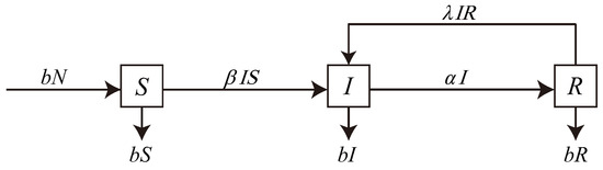
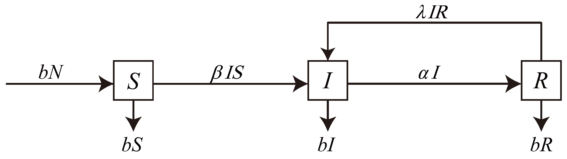
The System (7) simplifies the details of transmission, we can see the propagation process as shown in the figure below (see Figure 2).

Figure 2. Transfer diagram for SIRI model with reinfection.

Denote ${\mathsf{\Omega }}_1=\{(S,I,R):S+I+R=K,S\ge 0,I\ge 0,R\ge 0\}$, where $K=S\left(0\right)+I\left(0\right)+R\left(0\right)$. Obviously, if $S\left(0\right)\ge 0$, $I\left(0\right)\ge 0$, $R\left(0\right)\ge 0$, ${\mathsf{\Omega }}_1$ is positive invariant with respect to System (7).

3.1. The Basic Reproduction Number

Considering the effect of the initial number $I\left(0\right)$, the total number of infectious individuals at time t of System (7) is given by

$$\begin{array}{c}\hfill I\left(t\right)={\int }_0^t[\beta I\left(t_0\right)S\left(t_0\right)+\lambda I\left(t_0\right)R\left(t_0\right)]e^{-(\alpha +b)(t-t_0)}d{t}_0+I\left(0\right)e^{-(\alpha +b)t}.\end{array}$$

(8)

The term $\beta I\left(t_0\right)S\left(t_0\right)+\lambda I\left(t_0\right)R\left(t_0\right)$ represents the new growth rate of the infectious $\left(I\right)$ class at time $t_0$. The term $[\beta I\left(t_0\right)S\left(t_0\right)+\lambda I\left(t_0\right)R\left(t_0\right)]e^{-(\alpha +b)(t-t_0)}$ accounts for the number of newly infectious individuals at time $t_0$ who survive and have not recovered until time t. The term $I\left(0\right)e^{-(\alpha +b)t}$ represents the number of individuals remaining in the infectious stage at time t from the initial infectious population $I\left(0\right)$.

Consider the early stage of disease invasion, at this time $S\left(t_0\right)\approx K$ (almost all of them are susceptible), $R\left(t_0\right)\approx 0$. In order to analyze the number of new infections generated by an initial infected person throughout the entire infectious period, we ignore $\lambda I\left(t_0\right)R\left(t_0\right)$ and $I\left(0\right)e^{-(b+\alpha )t}$. The Formula (8) is simplified to

$$I\left(t\right)\approx {\int }_0^t\beta I\left(t_0\right)S\left(t_0\right)e^{-(\alpha +b)(t-t_0)}d{t}_0.$$

The Basic Reproduction Number, denoted as $R_0$, is defined as the average number of secondary infections produced by a single infected individual in a completely susceptible population.

$$\begin{array}{c}\hfill R_0=\beta K{\int }_0^{\infty }{e}^{-(\alpha +b)\tau }d\tau ={\displaystyle \frac{\beta K}{\alpha +b}}.\end{array}$$

(9)

Consequently, the basic reproduction number of the periodic System (2) can be computed as a period average,

$${\mathcal{R}}_0={\displaystyle \frac{K}{\alpha +b}}{\displaystyle \frac{1}{\omega }}{\int }_0^{\omega }\overline{\beta }\left(t\right)dt,$$

which coincides with the basic reproduction number of the corresponding averaged System (7)

$$R_0={\displaystyle \frac{\beta K}{\alpha +b}},\beta ={\displaystyle \frac{1}{\omega }}{\int }_0^{\omega }\overline{\beta }\left(t\right)dt.$$

This demonstrates that the averaged system not only provides a simple and explicit estimate of the basic reproduction number but also captures the long-term dynamical threshold of the original periodic system. In particular, it justifies using the average transmission rate to obtain preliminary parameter estimates and to assess the epidemic threshold in a periodically varying environment.

3.2. Existence of Equilibria

Considering that the total number of population is constant K, the system is reduced to a two-dimensional system, then System (7) can be rewritten as the following equivalent system:

$$\left\{\begin{array}{cc}\hfill \dot{S}& =bK-\beta SI-bS,\hfill \\ \hfill \dot{I}& =I\left[\right(\beta -\lambda )S-\lambda I+\lambda K-\alpha -b],\hfill \end{array}\right.$$

(10)

in a two-dimensional feasible region ${\mathsf{\Omega }}_2=\{(S,I):0\le S+I\le K,S\ge 0,I\ge 0\}$. Region ${\mathsf{\Omega }}_2$ is positive invariant with respect to System (10). In the rest of the paper, we will study the dynamics of System (10) with the initial conditions $S\left(0\right)>0,I\left(0\right)>0$ in region ${\mathsf{\Omega }}_2$.

In order to obtain the equilibria of System (10), let the right hand side of (10) be equal to zero:

$$\left\{\begin{array}{cc}\hfill bK-\beta SI-bS& =0,\hfill \\ \hfill I\left[\right(\beta -\lambda )S-\lambda I+\lambda K-\alpha -b]& =0,\hfill \end{array}\right.$$

(11)

Obviously, there always exists the boundary equilibrium $E_0(K,0)$. The positive equilibria of (10) are determined by equation

$$\left\{\begin{array}{c}\hfill bK-\beta SI-bS=0,\\ \hfill (\beta -\lambda )S-\lambda I+\lambda K-\alpha -b=0.\end{array}\right.$$

(12)

From the first equation of (12), we can obtain $S={\displaystyle \frac{bK}{\beta I+b}}$, then, put it into the second equation and give the single equation

$$-{\displaystyle \frac{1}{\beta I+b}}[\lambda \beta I^2+(\lambda b+\beta (\alpha +b-\lambda K))I+b(\alpha +b-\beta K)]=0.$$

(13)

Denote $f\left(I\right)=A{I}^2+BI+C$, where $A=\lambda \beta$, $B=\lambda b+\beta (\alpha +b-\lambda K)$, $C=b(\alpha +b-\beta K)$. It is obvious that $E_0(K,0)$ is always an equilibrium of System (10). The positive equilibria $E_i^{*}(S\left(I_i^{*}\right),I_i^{*})$ of (10) are determined by equations $f\left(I_i^{*}\right)=0$ and $S\left(I_i^{*}\right)={\displaystyle \frac{bK}{\beta I_i^{*}+b}}$. Then, we can find that $f\left(I\right)$ is upward parabolic, $I=-{\displaystyle \frac{B}{2A}}$ is symmetry axis, $f\left(0\right)=C$, $f\left(K\right)>0$, $f\left(K\right)-f\left(0\right)>0$. Based on the properties of the function $f\left(I\right)$, we investigate the existence of positive equilibria in the interior of ${\mathsf{\Omega }}_2$, and the corresponding results are summarized in the following theorem

Theorem 2. 

Let $R_0={\displaystyle \frac{\beta K}{\alpha +b}}$, for the System (10) the boundary equilibrium $E_0(K,0)$ always exists, and the following are true.

(1) If $R_0<1$, $B<0$, $\Delta >0$, there exist two positive equilibria $E_1^{*}(S\left(I_1^{*}\right),I_1^{*})$ and $E_2^{*}(S\left(I_2^{*}\right),I_2^{*})$, where $I_1^{*}={\displaystyle \frac{-B-\sqrt{\Delta }}{2A}}$, $I_2^{*}={\displaystyle \frac{-B+\sqrt{\Delta }}{2A}}$, and $I_1^{*}<-{\displaystyle \frac{B}{2A}}<I_2^{*}$.

(2) If $R_0<1$, $B<0$, $\Delta =0$, there exist a unique positive equilibrium $E_3^{*}(S\left(I_3^{*}\right),I_3^{*})$, where $I_3^{*}=-{\displaystyle \frac{B}{2A}}$.

(3) If $R_0=1$, $B<0$, there exist a unique positive equilibrium $E_4^{*}(S\left(I_4^{*}\right),I_4^{*})$, where $I_4^{*}={\displaystyle \frac{-B+\sqrt{\Delta }}{2A}}$, and $I_4^{*}>-{\displaystyle \frac{B}{2A}}$.

(4) If $R_0>1$, there exist a unique positive equilibrium $E_5^{*}(S\left(I_5^{*}\right),I_5^{*})$, $I_5^{*}={\displaystyle \frac{-B+\sqrt{\Delta }}{2A}}$, and $I_5^{*}>-{\displaystyle \frac{B}{2A}}$.

(5) There is no positive equilibrium except the above cases, where $\Delta =B^2-4AC$, $E_i^{*}(S\left(I_i^{*}\right),I_i^{*})$ satisfy the equations $f\left(I_i^{*}\right)=0$ and $S\left(I_i^{*}\right)={\displaystyle \frac{bK}{\beta I_i^{*}+b}}$.

Furthermore, we find that $B<0$ is equivalent to $R_1:={\displaystyle \frac{\lambda \beta K}{\lambda b+\beta (\alpha +b)}}>1$, $\Delta \ge 0$ is equivalent to $\alpha \le {\displaystyle \frac{b\lambda -\sqrt{4\beta (\lambda -\beta )b\lambda K}}{\beta }}+\lambda K-b=:{\alpha }_c$. Denote $R_0^c=R_0{|}_{R_0<1,B<0,\Delta =0}$, we can know

$$R_0^c={\displaystyle \frac{\beta K}{{\alpha }_c+b}}={\displaystyle \frac{{\beta }^{2}K}{b\lambda +\lambda \beta K-\sqrt{4\beta (\lambda -\beta )b\lambda K}}},$$

and $0<R_0^c<1$. $\alpha <{\alpha }_c$ is equivalent to $R_0>R_0^c$. We obtain that Theorem 2 is equivalent to the following theorem. The above conditions are settled in Table 1.

Table 1. Conditions for the existence of equilibria.

Case	Condition	Equivalent Condition	Positive Equilibria
$R_0<1$	$B<0,\Delta >0$	$R_1>1,R_0^c<R_0<1$	$E_1^{*},E_2^{*}$
	$B<0,\Delta =0$	$R_1>1,R_0^c=R_0<1$	$E_3^{*}$
	$B<0,\Delta <0$	$R_1>1,R_0<R_0^c<1$	None
	$B=0$	$R_1=1$	None
	$B>0$	$R_1<1$	None
$R_0=1$	$B<0$	$R_1>1$	$E_4^{*}$
	$B=0$	$R_1=1$	None
	$B>0$	$R_1<1$	None
$R_0>1$	–	–	$E_5^{*}$

Theorem 3. 

Let $R_0={\displaystyle \frac{\beta K}{\alpha +b}}$, $R_1={\displaystyle \frac{\lambda \beta K}{\lambda b+\beta (\alpha +b)}}$, $R_0^c=R_0{|}_{R_0<1,B<0,\Delta =0}$ for the System (10) the boundary equilibrium $E_0(K,0)$ always exists, and the following are true.

(1) If $R_0<1$, $R_1>1$, $R_0^c<R_0<1$, there exist two positive equilibria $E_1^{*}(S\left(I_1^{*}\right),I_1^{*})$ and $E_2^{*}(S\left(I_2^{*}\right),I_2^{*})$.

(2) If $R_0<1$, $R_1>1$, $R_0^c=R_0<1$, there exist a unique positive equilibrium $E_3^{*}(S\left(I_3^{*}\right),I_3^{*})$.

(3) If $R_0=1$, $R_1>1$, there exist a unique positive equilibrium $E_4^{*}(S\left(I_4^{*}\right),I_4^{*})$.

(4) If $R_0>1$, there exists a unique positive equilibrium $E_5^{*}(S\left(I_5^{*}\right),I_5^{*})$.

(5) There is no positive equilibrium except the above cases, where $\Delta =B^2-4AC$, $E_i^{*}(S\left(I_i^{*}\right),I_i^{*})$ satisfy the equations $f\left(I_i^{*}\right)=0$ and $S\left(I_i^{*}\right)={\displaystyle \frac{bK}{\beta I_i^{*}+b}}$.

3.3. Stability Analysis

Theorem 4. 

Let $R_0={\displaystyle \frac{\beta K}{\alpha +b}}$, $R_1={\displaystyle \frac{\lambda \beta K}{\lambda b+\beta (\alpha +b)}}$, for the System (10) the boundary equilibrium $E_0(K,0)$ always exists, and the following are true.

(1) The boundary equilibrium $E_0$ is a stable node if $R_0<1$ and $E_0$ is a saddle point if $R_0>1$. In the case of $R_0=1$, $E_0$ is unstable if $R_1>1$ and $E_0$ is locally asymptotically stable if $R_1\le 1$.

(2) If $E_1^{*}$ and $E_2^{*}$ exist, $E_1^{*}$ is a saddle point, $E_2^{*}$ is locally asymptotically stable.

(3) If $E_3^{*}$ exists, $E_3^{*}$ is saddle node.

(4) If $E_4^{*}$ exists, $E_4^{*}$ is locally asymptotically stable.

(5) If $E_5^{*}$ exists, $E_5^{*}$ is locally asymptotically stable.

Proof of Theorem 4. 

The Jacobian matrix of System (10) at an equilibrium $(S,I)$ is

$$J=\left[\begin{array}{cc}-\beta I-b& -\beta S\\ (\beta -\lambda )I& (\beta -\lambda )S-2\lambda I+\lambda K-\alpha -b\end{array}\right].$$

(14)

We study the stability of positive equilibria in the following three cases.

Case 1: Because of the boundary equilibrium conditions, the matrix at $E_0$ is

$$J\left(E_0\right)=\left[\begin{array}{cc}-b& -\beta K\\ 0& \beta K-\alpha -b\end{array}\right].$$

(15)

It is easy to obtain that the eigenvalue is ${\widehat{\lambda }}_1=-b<0$, ${\widehat{\lambda }}_2=\beta K-\alpha -b$. In the case of $R_0<1$, ${\widehat{\lambda }}_2<0$, $E_0$ is a stable node. In the case of $R_0>1$, ${\widehat{\lambda }}_2>0$, $E_0$ is a saddle point. In the case of $R_0=1$, it is equivalent to $\beta K=\alpha +b$, then ${\widehat{\lambda }}_2=0$. In order to determine the distribution of orbits of (10) near $E_0$, we take the transformation as follows.

$$\left\{\begin{array}{cc}\hfill u& =I,\hfill \\ \hfill v& =\beta KI+b(S-K),\hfill \\ \hfill x& =-t.\hfill \end{array}\right.$$

(16)

Then System (10) becomes

$$\left\{\begin{array}{cc}\hfill {\displaystyle \frac{du}{dx}}& =-u[{\displaystyle \frac{\beta -\lambda }{b}}v-({\displaystyle \frac{\beta K(\beta -\lambda )}{b}}+\lambda )u],\hfill \\ \hfill {\displaystyle \frac{dv}{dx}}& =bv+\beta Ku[({\displaystyle \frac{1}{K}}-{\displaystyle \frac{\beta -\lambda }{b}})v+({\displaystyle \frac{\beta K(\beta -\lambda )}{b}}+\lambda -\beta )u].\hfill \end{array}\right.$$

(17)

Let the right side of the second equation of (17) equal to zero, then we have

$$\begin{array}{c}\hfill v=a_1{u}^2+{\left[u\right]}_2,a_1={\displaystyle \frac{\beta K}{b^2}}(\lambda -\beta )(\beta K-b)={\displaystyle \frac{\alpha \beta K}{b^2}}(\lambda -\beta ),\end{array}$$

(18)

where ${\left[u\right]}_m$ represents the sum of the terms of which the orders are greater than m. Substituting (18) into the first equation of (17) gives

$$\begin{array}{c}\hfill {\displaystyle \frac{du}{dx}}=\left\{\begin{array}{cc}\hfill & {\displaystyle \frac{B}{b}}{u}^2+{\left[u\right]}_2,B\ne 0,\hfill \\ \hfill & {\displaystyle \frac{\alpha \beta K{(\lambda -\beta )}^2}{b^3}}{u}^3+{\left[u\right]}_3,B=0.\hfill \end{array}\right.\end{array}$$

(19)

By Theorem 7.1 in [30] and negative vector field, let us analyse the stability of $E_0$ in three cases.

In the case of $B>0$, the image of (10) is approaches to $E_0$ in the interior of ${\mathsf{\Omega }}_2$.

In the case of $B<0$, the image of (10) is away from $E_0$ in the interior of ${\mathsf{\Omega }}_2$.

In the case of $B=0$, it is easy to obtain $\lambda b=-\beta K(\beta -\lambda )$, because of $b>0$, so we can find $\beta <\lambda$, then ${\displaystyle \frac{\alpha \beta K{(\lambda -\beta )}^2}{b^3}}>0$, so the image of (10) is approaches to $E_0$ in the interior of ${\mathsf{\Omega }}_2$.

Hence, $E_0$ is unstable if $B<0$ and $E_0$ is locally asymptotically stable if $B\ge 0$ in the interior of ${\mathsf{\Omega }}_2$.

Case 2: The matrix at $E_i^{*}$ is

$$J\left(E_i^{*}\right)=\left[\begin{array}{cc}-\beta I_i^{*}-b& -\beta S_i^{*}\\ (\beta -\lambda )I_i^{*}& -\lambda I_i^{*}\end{array}\right].$$

(20)

It is easy to obtain that

$$\begin{array}{cc}\hfill trJ\left(E_i^{*}\right)& ={\overline{\lambda }}_1+{\overline{\lambda }}_2=-((\lambda +\beta )I_i^{*}+b)<0,\hfill \\ \hfill detJ\left(E_i^{*}\right)& ={\overline{\lambda }}_1{\overline{\lambda }}_2=2A{I}_i^{*}(I_i^{*}+{\displaystyle \frac{B}{2A}}).\hfill \end{array}$$

(21)

By Theorem 2, $I_1^{*}<-{\displaystyle \frac{B}{2A}}$, $I_3^{*}=-{\displaystyle \frac{B}{2A}}$, $I_j^{*}>-{\displaystyle \frac{B}{2A}}$, where $j=2,4,5$. If $E_i^{*}$ exists, we have $detJ\left(E_1^{*}\right)<0$, $detJ\left(E_3^{*}\right)=0$, $detJ\left(E_j^{*}\right)>0$. Hence, $E_1^{*}$ is a saddle point, $E_j^{*}$ is locally asymptotically stable.

Now, we will analyse the stability of $E_3^{*}$. In order to determine the distribution of orbits of (10) near $E_3^{*}$, we take the transformation

$$\left\{\begin{array}{cc}\hfill u& ={\displaystyle \frac{1}{\lambda I_3^{*}+\beta I_3^{*}+b}}[{\displaystyle \frac{\beta I_3^{*}+b}{I_3^{*}(\beta -\lambda )}}(I-I_3^{*})+(S-S_3^{*})],\hfill \\ \hfill v& =u-{\displaystyle \frac{I-I_3^{*}}{I_3^{*}(\beta -\lambda )}},\hfill \\ \hfill \tau & =-t.\hfill \end{array}\right.$$

(22)

Then (10) becomes

$$\left\{\begin{array}{cc}\hfill {\displaystyle \frac{du}{d\tau }}& ={\displaystyle \frac{\beta -\lambda }{\lambda I_3^{*}+\beta I_3^{*}+b}}[\lambda \beta {\left(I_3^{*}\right)}^2{u}^2+D_1{v}^2-D_{2}uv],\hfill \\ \hfill {\displaystyle \frac{dv}{d\tau }}& =(\lambda I_3^{*}+\beta I_3^{*}+b)v+{\displaystyle \frac{(\beta -\lambda )\lambda \beta }{\lambda I_3^{*}+\beta I_3^{*}+b}}{\left(I_3^{*}\right)}^2{u}^2+D_3{v}^2+D_{4}uv,\hfill \end{array}\right.$$

(23)

where

$$\begin{array}{cc}\hfill D_1& =(\beta I_3^{*}+b)(\lambda I_3^{*}+b),\hfill \\ \hfill D_2& =(\beta I_3^{*}+b)(\lambda I_3^{*}+b)+\lambda \beta {\left(I_3^{*}\right)}^2,\hfill \\ \hfill D_3& ={\displaystyle \frac{(\beta -\lambda )(\beta I_3^{*}+b)(\lambda I_3^{*}+b)}{\lambda I_3^{*}+\beta I_3^{*}+b}}-(\lambda I_3^{*}+\beta I_3^{*}+b)(\beta -\lambda ),\hfill \\ \hfill D_4& =-{\displaystyle \frac{\beta -\lambda }{\lambda I_3^{*}+\beta I_3^{*}+b}}[(\beta I_3^{*}+b)(\lambda I_3^{*}+b)+\lambda \beta {\left(I_3^{*}\right)}^2]+(\lambda I_3^{*}+\beta I_3^{*}+b)(\beta -\lambda ).\hfill \end{array}$$

Let the right side of the second equation of (23) equal to zero, then we have

$$\begin{array}{c}\hfill v=a_2{u}^2+{\left[u\right]}_2,a_2=-{\displaystyle \frac{(\beta -\lambda )\lambda \beta }{{(\lambda I_3^{*}+\beta I_3^{*}+b)}^2}}{\left(I_3^{*}\right)}^2,\end{array}$$

(24)

where ${\left[u\right]}_2$ represents the sum of the terms of which the orders are greater than two.

Substituting (24) into the first equation of (23) gives

$${\displaystyle \frac{du}{d\tau }}={\displaystyle \frac{(\beta -\lambda )\lambda \beta {\left(I_3^{*}\right)}^2}{\lambda I_3^{*}+\beta I_3^{*}+b}}{u}^2+{\left[u\right]}_2.$$

Since the condition of existence of $E_3^{*}$, we know $B<0$ and $R_0<1$. It is easy to obtain $\beta K<\alpha +b<-{\displaystyle \frac{\lambda b}{\beta }}+\lambda K$, so we can find $\lambda >\beta$, then ${\displaystyle \frac{(\beta -\lambda )\lambda \beta {\left(I_3^{*}\right)}^2}{\lambda I_3^{*}+\beta I_3^{*}+b}}<0$. By [30] (Theorem 7.1) and negative vector field, $E_3^{*}$ is saddle node. The neighborhood of the equilibrium point is divided into two parts by the dividing line, one is a parabolic sector and the other is two hyperbolic sectors. Parabolic sector orbits tend to the equilibrium point, hyperbolic sector orbits away from the equilibrium point. □

Theorem 5. 

There is no periodic solution for system (10).

Proof of Theorem 5. 

Rewrite (10) as

$$\left\{\begin{array}{cc}\hfill \dot{S}& =bK-\beta SI-bS=P(S,I),\hfill \\ \hfill \dot{I}& =I\left[\right(\beta -\lambda )S-\lambda I+\lambda K-\alpha -b]=Q(S,I).\hfill \end{array}\right.$$

(25)

Let $\phi (S,I)={\displaystyle \frac{1}{I}}$ be a Dulac multiplier. Then

$${\displaystyle \frac{\partial \left(\phi P\right)}{\partial S}}+{\displaystyle \frac{\partial \left(\phi Q\right)}{\partial I}}=-(\beta +{\displaystyle \frac{b}{I}}+\lambda )<0.$$

(26)

Therefore, the Bendixson-Dulac condition [31] holds in the interior of ${\mathsf{\Omega }}_2$ and no periodic solutions exist in the interior of ${\mathsf{\Omega }}_2$. □

Summarizing the analyses from above, the following theorem is easily obtained.

Theorem 6. 

For System (10), the following results hold.

(1) If $R_0<1$, $R_1>1$, $R_0^c<R_0<1$, then there exist two stable manifolds of the equilibrium $E_1^{*}$, which divide the region ${\mathsf{\Omega }}_2$ into two parts $A_1$ and $A_2$, where $E_2^{*}\in A_1$, $E_2^{*}\notin A_2$, such that ${lim}_{t\to \infty }(S\left(t\right),I\left(t\right))=(S_2^{*},I_2^{*})$, when $(S_0,I_0)\in A_1$, and ${lim}_{t\to \infty }(S\left(t\right),I\left(t\right))=(K,0)$ when $(S_0,I_0)\in A_2$.

(2) If $R_0<1$, $R_1>1$, $R_0^c=R_0<1$, then there exists a separatrix of the equilibrium $E_3^{*}$, which divides the region ${\mathsf{\Omega }}_2$ into two parts $B_1$ and $B_2$, where $E_3^{*}\in B_1$, $E_3^{*}\notin B_2$, such that ${lim}_{t\to \infty }(S\left(t\right),I\left(t\right))=(S_3^{*},I_3^{*})$, when $(S_0,I_0)\in B_1$, and ${lim}_{t\to \infty }(S\left(t\right),I\left(t\right))=(K,0)$ when $(S_0,I_0)\in B_2$.

(3) If $R_0=1$, $R_1>1$, $E_4^{*}$ is globally asymptotically stable, $E_0$ is unstable.

(4) If $R_0>1$, $E_5^{*}$ is globally asymptotically stable, $E_0$ is unstable.

(5) If the parameters of (10) do not satisfy the cases of (1)–(4), the $E_0$ is globally asymptotically stable.

3.4. The Backward Bifurcation

By Theorem 2, if the positive equilibrium $E_i^{*}$ exists, then $2A{I}_1^{*}+B<0$, $2A{I}_3^{*}+B=0$, $2A{I}_j^{*}+B>0$, as $j=2,4,5$. Furthermore, $E_1^{*}$ is a saddle point which is unstable. $E_j^{*}$ is locally asymptotically stable.

Theorem 7. 

For the System (10), consider $R_0$ as the bifurcation parameter, we have that there exists a backward bifurcation if and only if $R_0^c<R_0<1$. Consider implicit differentiation of the equilibrium condition $f\left(I\right)=0$, if $2AI+B>0$, the bifurcation curve has positive slope at equilibrium values and the equilibrium is asymptotically stable. If $2AI+B<0$, the bifurcation curve has negative slope at equilibrium values and the equilibrium is unstable.

Proof of Theorem 7. 

From Theorem 3, we have that there exists a backward bifurcation if and only if $R_0^c<R_0<1$, where $R_0$ is the bifurcation parameter.

Implicit differentiation of the equilibrium condition $f\left(I\right)=0$ with respect to $R_0$ is equivalent to $h\left(I\right)=0$, where $h\left(I\right)=A{I}^2+BI+C=\tilde{A}{I}^2+\tilde{B}I+\tilde{C}$, $\tilde{A}=\lambda \beta$,$\tilde{B}=\lambda b+\beta ({\displaystyle \frac{\beta K}{R_0}}-\lambda K)$, $\tilde{C}=b({\displaystyle \frac{\beta K}{R_0}}-\beta K)$. Obviously, $2AI+B=2\tilde{A}I+\tilde{B}$.

$$(2AI+B){\displaystyle \frac{dI}{d{R}_0}}=(2\tilde{A}I+\tilde{B}){\displaystyle \frac{dI}{d{R}_0}}=-{\displaystyle \frac{d\tilde{A}}{d{R}_0}}{I}^2-{\displaystyle \frac{d\tilde{B}}{d{R}_0}}I-{\displaystyle \frac{d\tilde{C}}{d{R}_0}}={\displaystyle \frac{{\beta }^{2}K}{R_0^2}}I+{\displaystyle \frac{b\beta K}{R_0^2}}>0$$

(27)

Then, we can find ${\displaystyle \frac{dI}{d{R}_0}}>0$ when $2AI+B>0$; ${\displaystyle \frac{dI}{d{R}_0}}<0$ when $2AI+B<0$.

By (27), we can obtain that if the positive equilibrium $E_i^{*}$ exists, $I_i^{*}$ actually increases with increasing $R_0$ when $2A{I}_i^{*}+B>0$, which implies that the bifurcation curve has positive slope at equilibrium values with $2AI+B>0$ and the equilibrium is asymptotically stable, as well as, $I_i^{*}$ decreases with increasing $R_0$ when $2A{I}_i^{*}+B<0$, which implies that the bifurcation curve has negative slope at equilibrium values with $2AI+B<0$ and the equilibrium is unstable. □

Theorem 8. 

For the System (10), consider α as the bifurcation parameter, we have that there exists a backward bifurcation if and only if $0<\beta K-b<\alpha <{\alpha }_c$. Consider implicit differentiation of the equilibrium condition $f\left(I\right)=0$, if $2AI+B>0$, the bifurcation curve has negative slope at equilibrium values and the equilibrium is asymptotically stable. If $2AI+B<0$, the bifurcation curve has positive slope at equilibrium values and the equilibrium is unstable.

Proof of Theorem 8. 

Implicit differentiation of the equilibrium condition $f\left(I\right)=0$ with respect to $\alpha$ gives

$$(2AI+B){\displaystyle \frac{dI}{d\alpha }}=-{\displaystyle \frac{dA}{d\alpha }}{I}^2-{\displaystyle \frac{dB}{d\alpha }}I-{\displaystyle \frac{dC}{d\alpha }}=-\beta I-b<0.$$

(28)

Then, we can find ${\displaystyle \frac{dI}{d\alpha }}<0$ when $2AI+B>0$; ${\displaystyle \frac{dI}{d\alpha }}>0$ when $2AI+B<0$.

From above, we can obtain that if the positive equilibrium $E_i^{*}$ exists, $I_i^{*}$ actually decreases with increasing $\alpha$ when $2A{I}_i^{*}+B>0$, which implies that the bifurcation curve has negative slope at equilibrium values with $2AI+B>0$ and the equilibrium is asymptotically stable, as well as, $I_i^{*}$ increases with increasing $\alpha$ when $2A{I}_i^{*}+B<0$, which implies that the bifurcation curve has positive slope at equilibrium values with $2AI+B<0$ and the equilibrium is unstable. □

4. Numerical Simulations

4.1. The Bifurcation with Bifurcation Parameter $R_0$ for System (10)

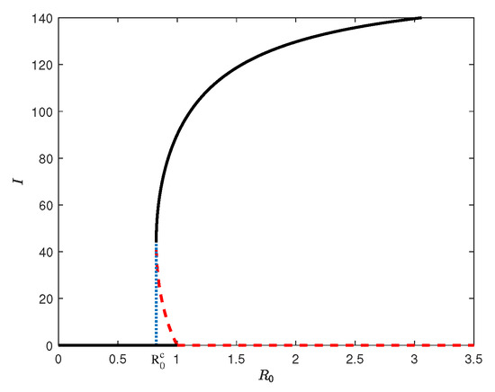
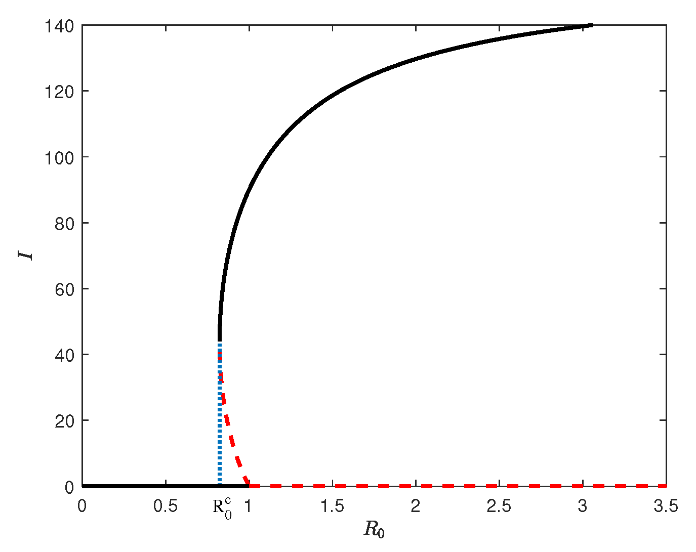
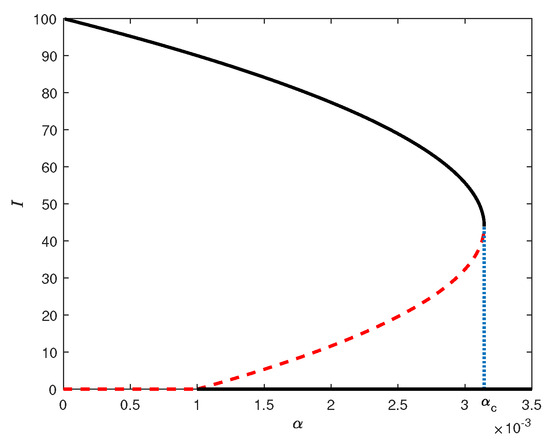
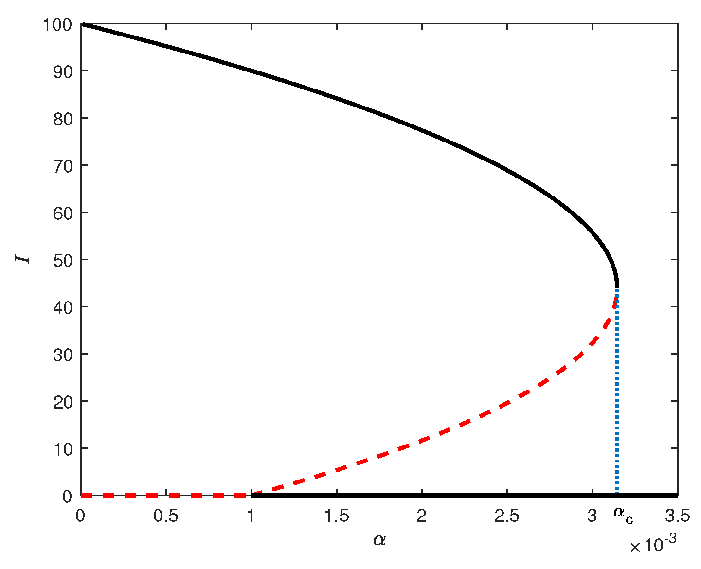
If there is a backward bifurcation when $R_0=1$, then the two positive equilibria given by $2AI+B=\pm \sqrt{\Delta }$, and the bifurcation curve has positive slope at $2AI+B>0$ and negative slope at equilibrium values with $2AI+B<0$. For example, with the parameter values $\beta =0.00001$, $\lambda =0.001$, $K=1000$, $b=0.009$, we have $R_0^c=0.8234$. Then the bifurcation curve is shown in Figure 3.

Figure 3. Backward bifurcation diagram of System (10) with respect to $R_0$. The system exhibits a backward bifurcation with two positive equilibria for $R_0^c<R_0<1$ under the parameter values $\beta =0.00001$, $\lambda =0.001$, $K=1000$, and $b=0.009$. The black solid curve denotes stable equilibria, the red dashed curve denotes unstable equilibria, and the blue dashed line indicates the bifurcation point $R_0^c$.

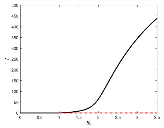
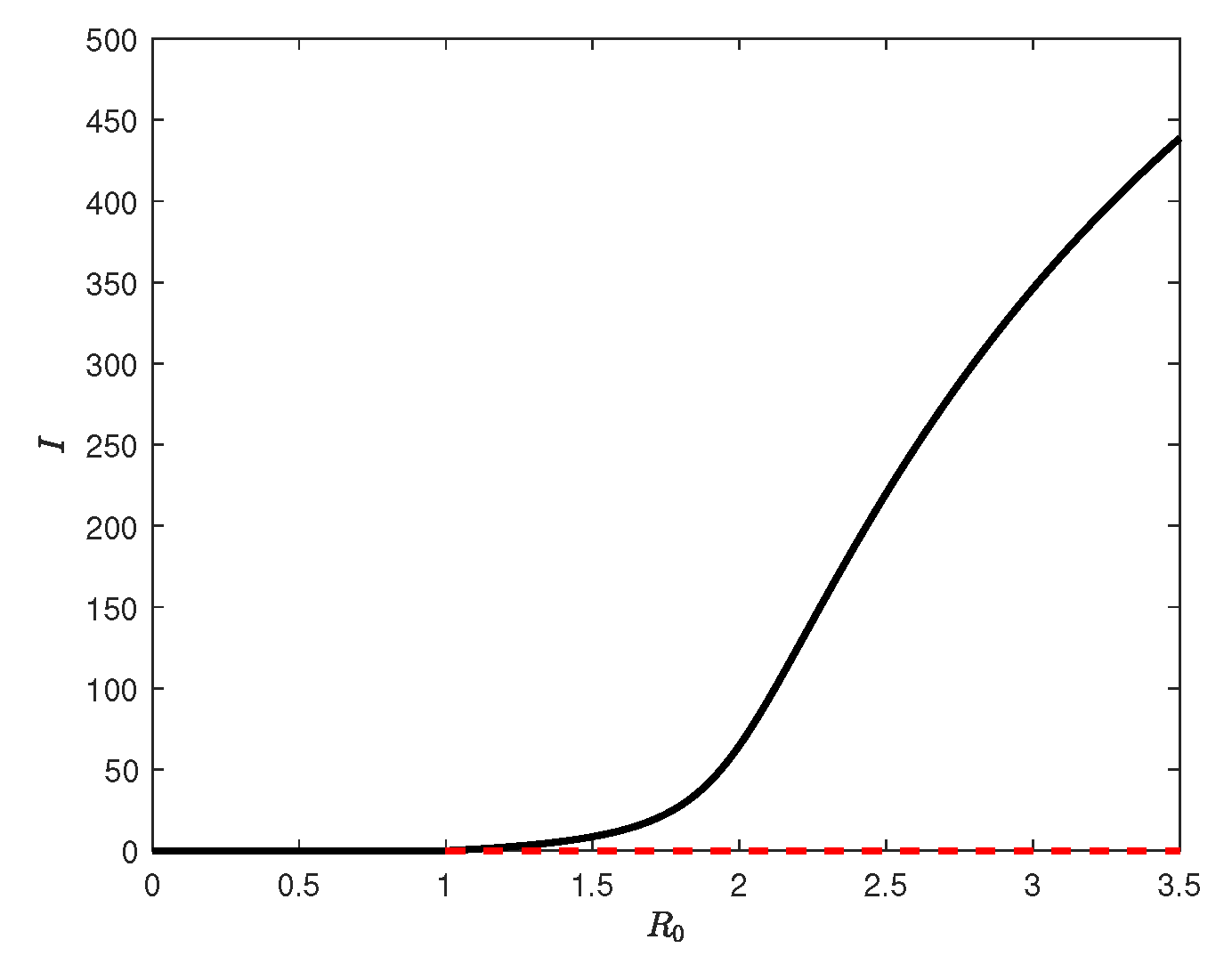
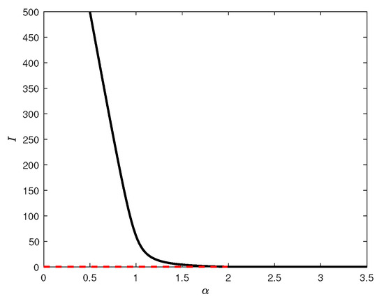
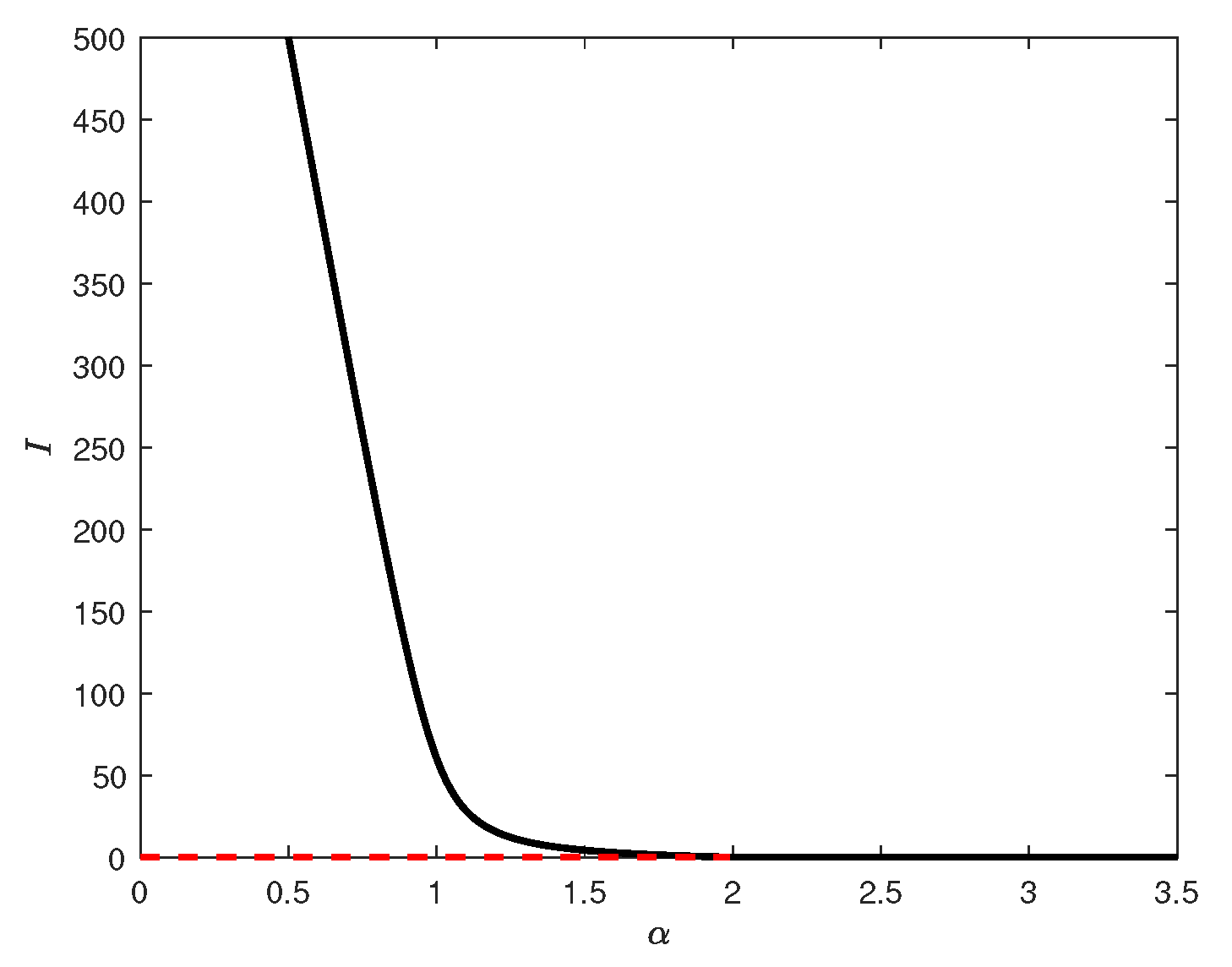
If there is not a backward bifurcation when the condition does not satisfy Theorem 7, and the unique positive equilibrium for $R_0>1$ satisfies $2AI+B>0$, and the bifurcation curve has positive slope at all points where $I>0$. For example, the parameter values are $\beta =0.002$, $\lambda =0.001$, $K=1000$, $b=0.009$. Then the bifurcation curve is shown in Figure 4.

Figure 4. Forward bifurcation diagram of System (10) with respect to $R_0$. The bifurcation at $R_0=1$ is forward, and a unique positive equilibrium exists for $R_0>1$ under the parameter values $\beta =0.002$, $\lambda =0.001$, $K=1000$, and $b=0.009$. The black solid curve denotes stable equilibria, the red dashed curve denotes unstable equilibria.

4.2. The Bifurcation with Bifurcation Parameter $\alpha$ for System (10)

Obviously, $R_0=1$ is equivalent to $\alpha =\beta K-b$, $R_0<1$ is equivalent to $\alpha >\beta K-b$. If there is a backward bifurcation when $\alpha =\beta K-b$, then the two positive equilibria given by $2AI+B=\pm \sqrt{\Delta }$, and the bifurcation curve has negative slope at $2AI+B>0$ and positive slope at equilibrium values with $2AI+B<0$. For example, with the parameter values $\beta =0.00001$, $\lambda =0.001$, $K=1000$, $b=0.009$, we have ${\alpha }_c=0.0031$ and $\beta K-b=0.001$. Then $R_0^c={\displaystyle \frac{\beta K}{{\alpha }_c+b}}=0.8234$. The bifurcation curve is shown in Figure 5.

Figure 5. Backward bifurcation diagram of System (10) with respect to $\alpha$. The system exhibits a backward bifurcation with two positive equilibria for $0<\beta K-b<\alpha <{\alpha }_c$ under the parameter values $\beta =0.00001$, $\lambda =0.001$, $K=1000$, and $b=0.009$. The black solid curve denotes stable equilibria, the red dashed curve denotes unstable equilibria, and the blue dashed line indicates the bifurcation point ${\alpha }_c$.

If there is not a backward bifurcation when the condition does not satisfy Theorem 8, and the unique positive equilibrium for $\alpha <\beta K-b$ satisfies $2AI+B>0$, and the bifurcation curve has negative slope at all points where $I>0$. For example, with the parameter values $\beta =0.002$, $\lambda =0.001$, $K=1000$, $b=0.009$, we have $\beta K-b=1.9910$. Then the bifurcation curve is shown in Figure 6.

Figure 6. Forward bifurcation diagram of System (10) with respect to $\alpha$. The system exhibits a forward bifurcation at $\alpha =\beta K-b$, and admits a unique positive equilibrium for $\alpha <\beta K-b$ under the parameter values $\beta =0.002$, $\lambda =0.001$, $K=1000$, and $b=0.009$. The black solid curve denotes stable equilibria, the red dashed curve denotes unstable equilibria.

4.3. The Phase Diagrams About Equilibria for System (10)

We start with some numerical evidence to suggest that System (10) can have a few stable or unstable equilibria.

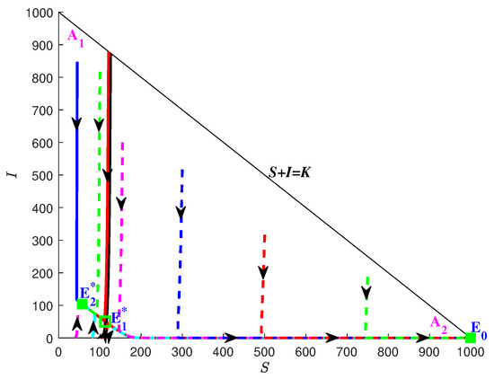
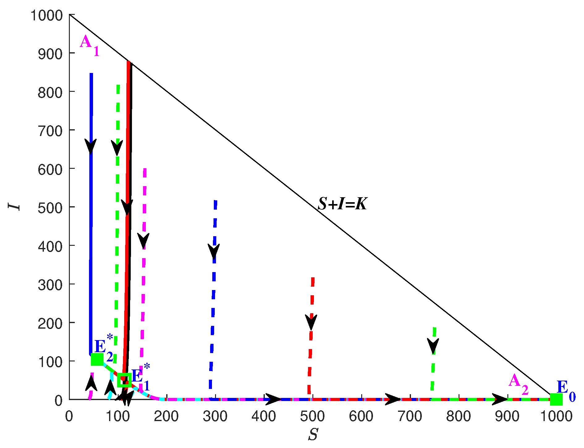
Figure 7 corresponds to the case $R_0<1$, $R_1>1$, $R_0^c<R_0<1$ with parameter values $K=1000$, $\alpha =0.84$, $\beta =0.00003$, $\lambda =0.001$, $b=0.00019$. System (10) have three equilibria $E_0(1000,0)$, $E_1^{*}(114.0161,49.2144)$ and $E_2^{*}(57.2657,104.2623)$. It is easy to obtain $R_0=0.0357$, $R_1=1.1813$, $R_0^c=0.0353$. The black curve which is the dividing line found by numerical simulation divides the region ${\mathsf{\Omega }}_2$ into two parts $A_1$ and $A_2$. $E_2^{*}$ (resp.$E_0$) is locally asymptotically stable in $A_1$ (resp.$A_2$). $E_1^{*}$ is a saddle point. Figure 7 shows that the bistable phenomenon that there exist two stable equilibria $E_0$ and $E_2^{*}$ which are consistent with the theoretical conclusion in Theorem 6.

Figure 7. Phase portrait of System (10) when $R_0<1$, $R_1>1$, and $R_0^c<R_0<1$. The system exhibits bistability. The equilibrium $E_1^{*}$ is a saddle point, whereas $E_2^{*}$ and $E_0$ are locally asymptotically stable. The black solid line denotes the separatrix dividing ${\mathsf{\Omega }}_2$ into two regions $A_1$ and $A_2$. Solution trajectories corresponding to different initial conditions are plotted in different colors. Solid rectangles denote stable equilibria, whereas hollow rectangles denote unstable equilibria. Arrows indicate the direction of trajectories.

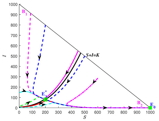
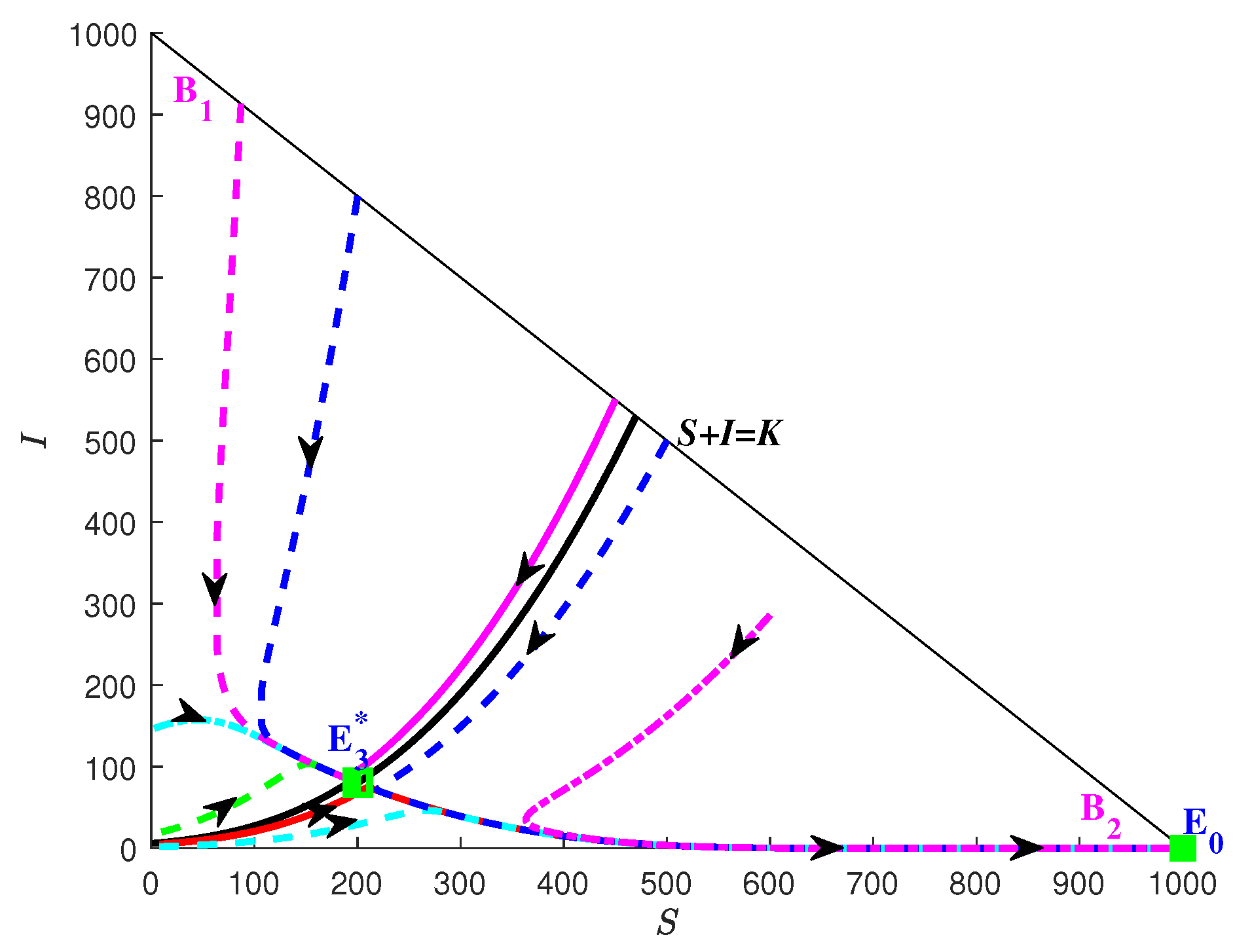
Figure 8 corresponds to the case $R_0<1$, $R_1>1$, $R_0^c=R_0<1$ with parameter values $K=1000$, $\alpha =0.1620$, $\beta =0.0001$, $\lambda =0.0002$, $b=0.002$. System (10) have two equilibria $E_0(1000,0)$, $E_3^{*}(200,80)$. It is easy to obtain $R_0=0.6098$, $R_1=1.1905$, $R_0^c=0.6098$. The black curve which is the dividing line found by numerical simulation divides the region ${\mathsf{\Omega }}_2$ into two parts $B_1$ and $B_2$. The trajectory depending on the initial conditions will tend to $E_3^{*}$ in $B_1$. $E_0$ is locally asymptotically stable in $B_2$. $E_3^{*}$ is saddle node. Figure 8 shows that $E_3^{*}$ is saddle node which are consistent with the theoretical conclusion in Theorem 6.

Figure 8. Phase portrait of System (10) when $R_0<1$, $R_1>1$, and $R_0=R_0^c<1$. The system admits two equilibria. The equilibrium $E_3^{*}$ is a saddle-node point, whereas $E_0$ is locally asymptotically stable. The black solid line denotes the separatrix dividing ${\mathsf{\Omega }}_2$ into two regions $B_1$ and $B_2$. Solution trajectories corresponding to different initial conditions are plotted in different colors. Solid rectangles denote stable equilibria, whereas half-filled rectangles denote saddle-node equilibria, which are stable from one side and unstable from the other. Arrows indicate the direction of the trajectories.

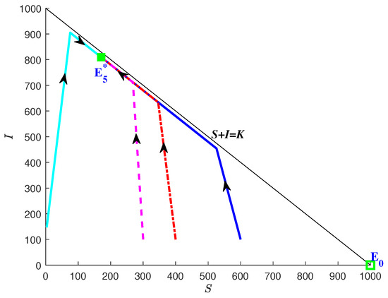
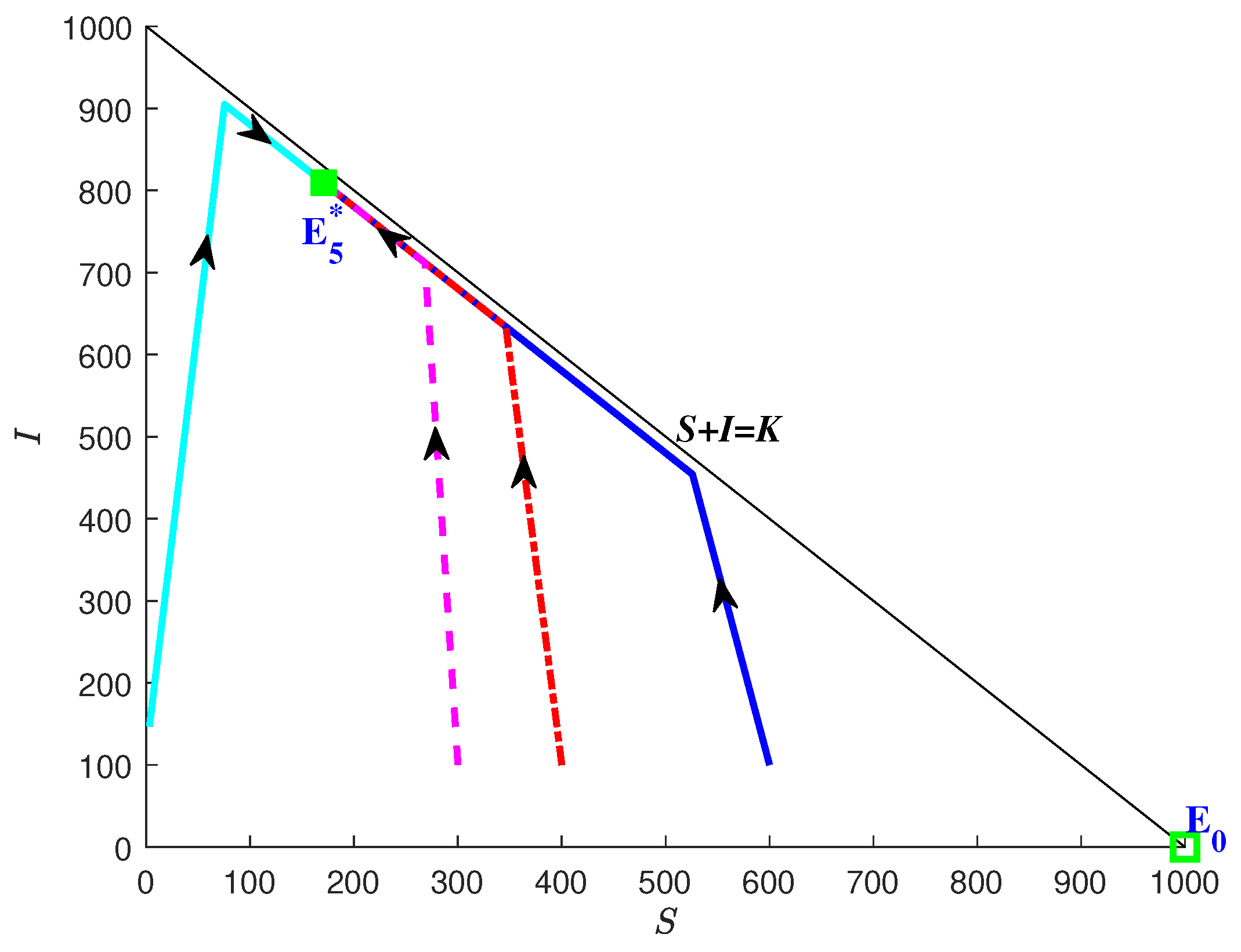
Figure 9 corresponds to the case $R_0=1$, $R_1>1$ with parameter values $K=1000$, $\alpha =0.2$, $\beta =0.0003$, $\lambda =0.01$, $b=0.1$. System (10) have two equilibria $E_0(1000,0)$, $E_4^{*}(343.6426,636.6667)$. It is easy to obtain $R_0=1$, $R_1=2.7523$. Figure 9 shows that $E_4^{*}$ is locally asymptotically stable and $E_0$ is unstable, which are consistent with the theoretical conclusion in Theorem 6.

Figure 9. Phase portrait of system (10) when $R_0=1$ and $R_1>1$. The system admits two equilibria. The equilibrium $E_4^{*}$ is locally asymptotically stable, whereas $E_0$ is unstable. Solution trajectories corresponding to different initial conditions are plotted in different colors. Solid rectangles denote stable equilibria, whereas hollow rectangles denote unstable equilibria. Arrows indicate the direction of trajectories.

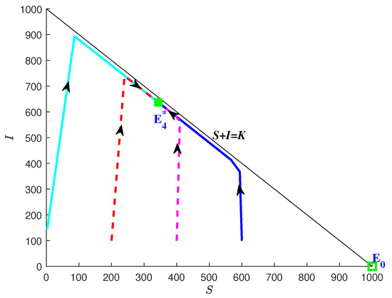
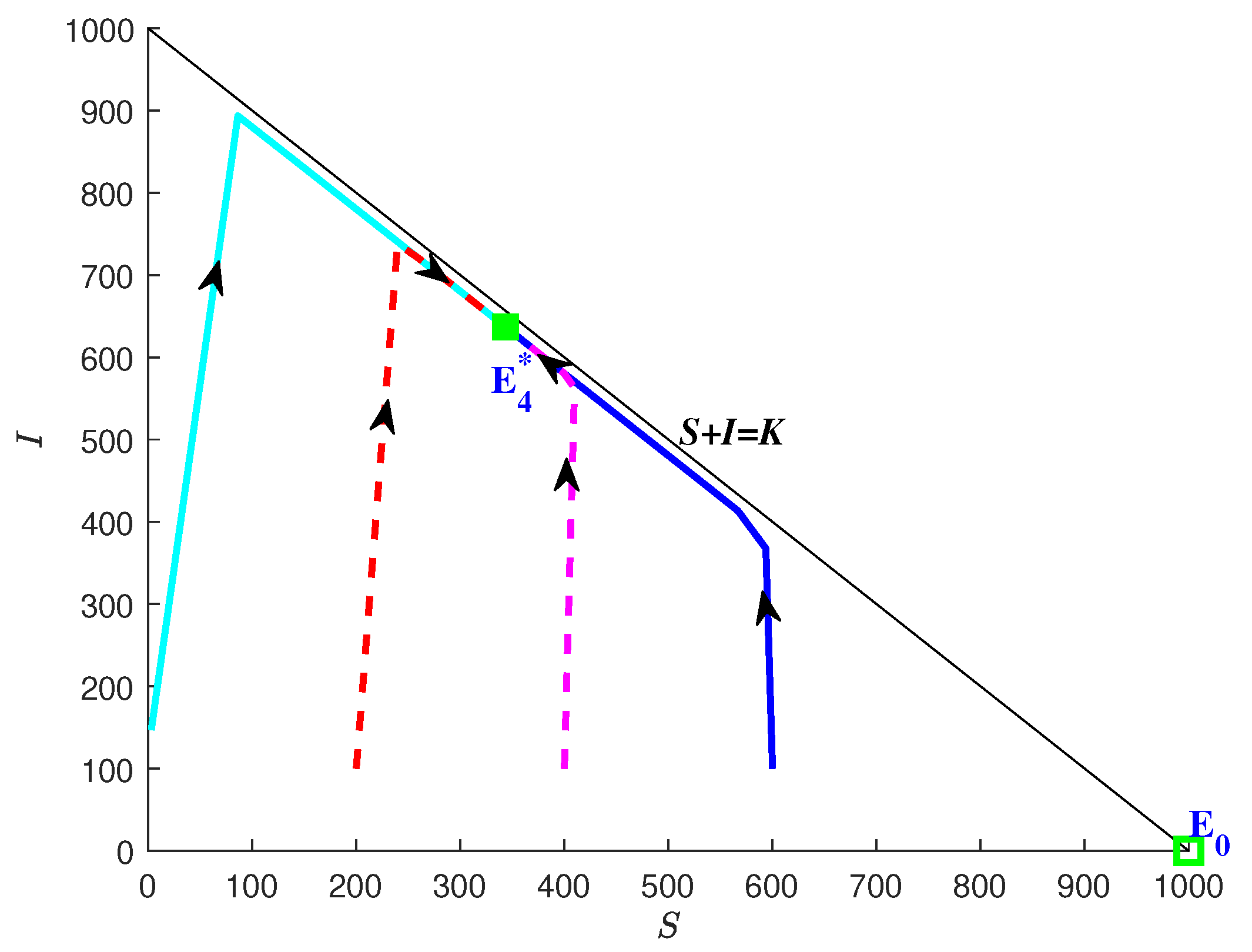
Figure 10 corresponds to the case $R_0>1$ with parameter values $K=1000$, $\alpha =0.4$, $\beta =0.0006$, $\lambda =0.02$, $b=0.1$. System (10) have two equilibria $E_0(1000,0)$, $E_5^{*}(170.7598,809.3629)$. It is easy to obtain $R_0=1.2$. Figure 10 shows that $E_5^{*}$ is locally asymptotically stable and $E_0$ is unstable, which are consistent with the theoretical conclusion in Theorem 6.

Figure 10. Phase portrait of System (10) when $R_0>1$. The system admits two equilibria. The equilibrium $E_5^{*}$ is locally asymptotically stable, whereas $E_0$ is unstable. Solution trajectories corresponding to different initial conditions are plotted in different colors. Solid rectangles denote stable equilibria, whereas hollow rectangles denote unstable equilibria. Arrows indicate the direction of trajectories.

4.4. A Case Study

Yunnan Province, a southwestern Chinese province bordering multiple high TB burden Greater Mekong Sub-region countries, has sustained relatively high TB notification rates and spatial clusters of disease, and continues to be prioritized in provincial TB control planning due to its significant TB burden [32].

From the Public Health Science Data Center [33], we obtained the monthly numbers of newly reported TB cases from January 2005 to December 2020. The monthly reported TB cases in Yunnan Province from 2005–2020 show an obvious seasonal fluctuation, indicating that seasonal forcing plays an important role in TB transmission dynamics. Demographic data and death rate date were taken from the China Statistical Yearbook published by the National Bureau of Statistics of China [34]. The average total population of Yunnan Province during 2005–2020 was used in the simulations, and the population size was fixed at $K=4.6175\times {10}^7$. Since the mortality rate data for Yunnan Province in 2020 were unavailable, we used the average mortality rate during 2005–2019, $\tilde{b}=6.43\times {10}^{-3}{\mathrm{year}}^{-1}$, in the simulations. The recovery rate was $\tilde{\alpha }=0.3743{\mathrm{year}}^{-1}$ [35].

In seasonal model, we assumed that

$$\overline{\beta }\left(t\right)={\beta }_0\left[1+a_{1}cos\left({\displaystyle \frac{2\pi (t+\tau )}{12}}+{\varphi }_1\right)+a_{2}cos\left({\displaystyle \frac{4\pi (t+\tau )}{12}}+{\varphi }_2\right)\right],$$

(29)

and

$$\overline{\lambda }\left(t\right)={\lambda }_0\left[1+a_{3}cos\left({\displaystyle \frac{2\pi (t+\tau )}{12}}+{\varphi }_3\right)\right],$$

(30)

where ${\beta }_0$ and ${\lambda }_0$ denote the mean transmission and reinfection rates, respectively; $a_i$ represent the amplitudes of seasonal forcing; ${\varphi }_i$ are the phase shifts; and $\tau$ is a time-shift parameter.

4.4.1. Sensitivity Analysis of $R_0$

Sensitivity analysis is important as it can be used for determining the parameters which are of most importance in reducing the level of a disease. The normalized forward sensitivity index of a variable to a parameter is the ratio of the relative change in the variable to the relative change in the parameter. The normalized forward sensitivity index [36] of a variable, $R_0$, that depends differentiably on a parameter, p, is defined as:

$$E_p={\displaystyle \frac{\partial R_0}{\partial p}}·{\displaystyle \frac{p}{R_0}}.$$

The sensitivity indices of $R_0$ with respect to the parameters $\beta$, $\alpha$, and b are given by

$$E_{\beta }=1,E_{\alpha }=-{\displaystyle \frac{\alpha }{\alpha +b}},E_b=-{\displaystyle \frac{b}{\alpha +b}}.$$

Substituting the annual parameter values of $\alpha =0.3743$ and $b=6.43\times {10}^{-3}$ into the above formulas yields the corresponding numerical sensitivity indices as

$$E_{\alpha }\approx -0.9831,E_b\approx -0.0169.$$

The results show that the basic reproduction number $R_0$ is most sensitive to the transmission rate $\beta$ and the recovery rate $\alpha$. In particular, the sensitivity index $E_{\beta }=1$ indicates that a $1\%$ increase in $\beta$ will lead to a $1\%$ increase in $R_0$. Similarly, the sensitivity index $E_{\alpha }\approx -0.9831$ implies that increasing the recovery rate $\alpha$ by $1\%$ will decrease $R_0$ by approximately $0.9831\%$. In contrast, the sensitivity index of the natural death rate b is relatively small ($E_b\approx -0.0169$), indicating that $R_0$ is much less sensitive to changes in b. The transmission rate and the recovery rate play dominant roles in the spread of the disease. These results suggest that reducing the transmission rate or increasing the recovery rate would be the most effective strategies for controlling the spread of the disease.

4.4.2. Comparison Between the Averaged and Seasonal Models

In this section, the monthly tuberculosis incidence data of Yunnan Province from 2005 to 2020 are used to estimate the unknown model parameters from the data and to compare the fitting performance of the two models. Since the demographic and epidemiological parameters are reported on a yearly scale, they are first converted into monthly units in order to match the time scale of the data. In particular, the natural mortality rate and the recovery rate are transformed as $b=\tilde{b}/12$, $\alpha =\tilde{\alpha }/12$.

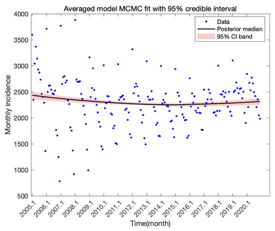
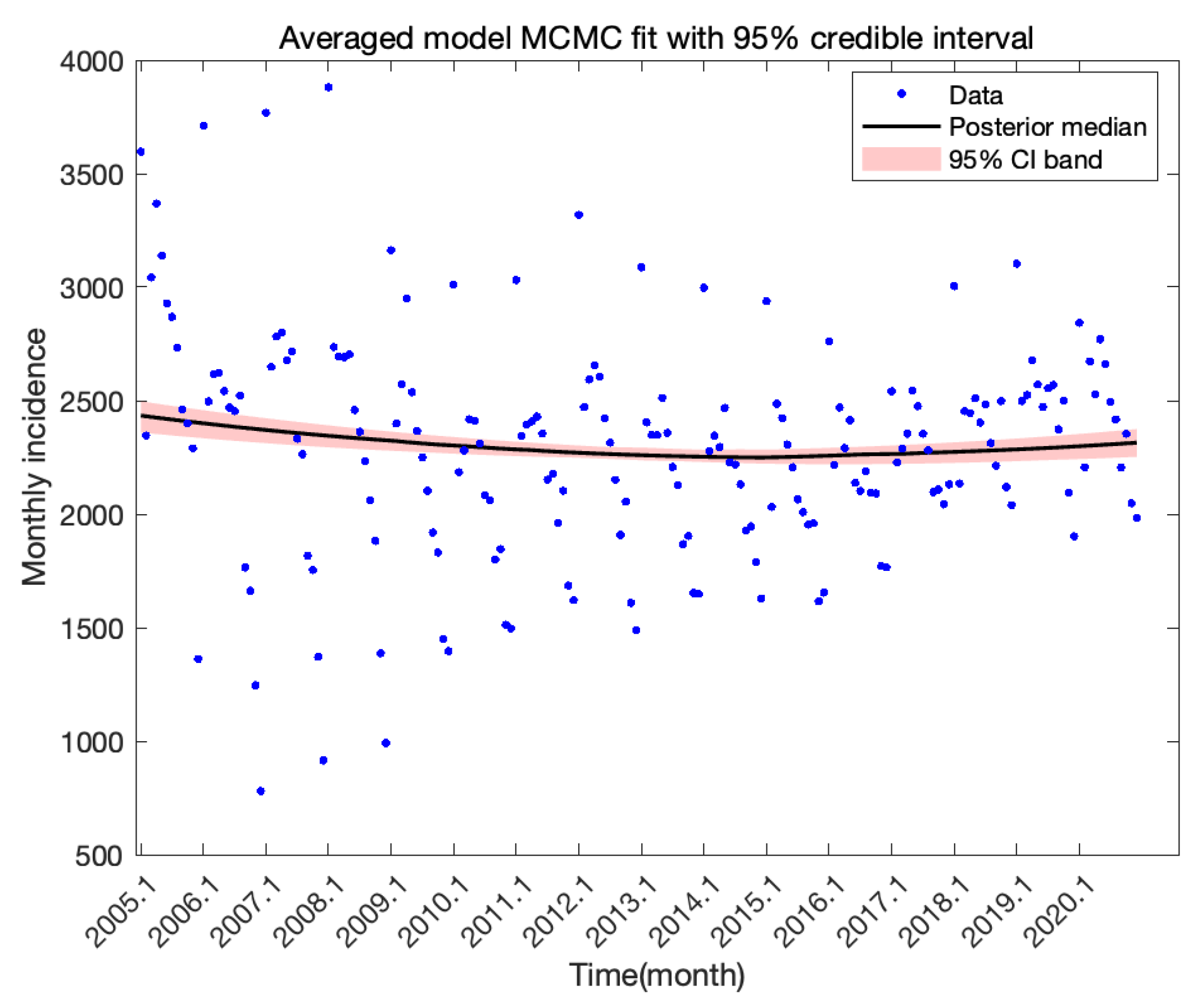
We first estimate the parameters $\beta$, $\lambda$, $S\left(0\right)$, and $I\left(0\right)$ of the averaged system using the Markov Chain Monte Carlo (MCMC) method. The MCMC procedure generates posterior distributions for the unknown parameters, from which the parameter confidence intervals can be obtained. The fitting results of the averaged system are presented in Figure 11. The 95% posterior predictive interval is relatively wider, reflecting the larger uncertainty of the averaged model in describing the observed data. The posterior means, medians, and 95% credible intervals of the model parameters estimated via the MCMC method for the averaged system are summarized in Table 2.

Figure 11. MCMC fit of monthly TB incidence in Yunnan (2005–2020) based on the averaged model with 95% credible interval.

Table 2. Posterior estimates of model parameters obtained by the MCMC method based on the averaged model.

Parameter	Mean	95% Credible Interval
$\beta$	$1.2279\times {10}^{-9}$	$[1.1760\times {10}^{-9},1.2701\times {10}^{-9}]$
$\lambda$	$2.8651\times {10}^{-11}$	$[8.7481\times {10}^{-12},4.8200\times {10}^{-11}]$
$S\left(0\right)$	$2.3959\times {10}^7$	$[2.3112\times {10}^7,2.5379\times {10}^7]$
$I\left(0\right)$	$8.1222\times {10}^4$	$[7.7594\times {10}^4,8.3313\times {10}^4]$

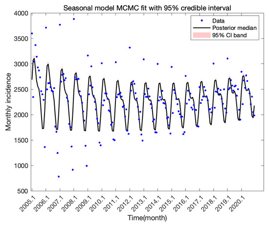
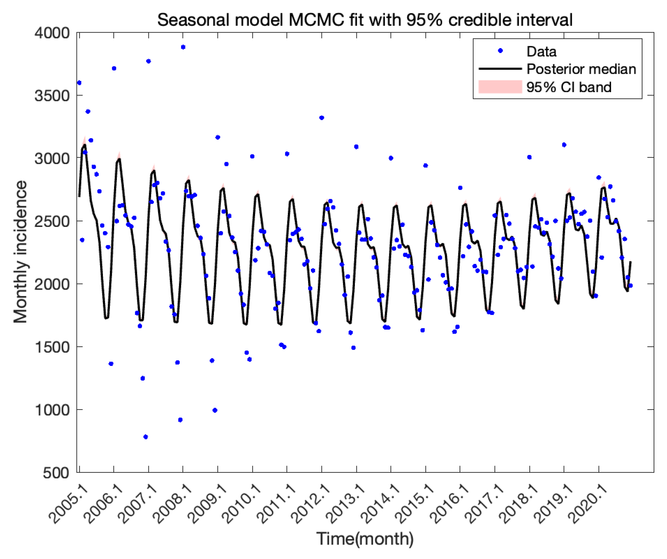
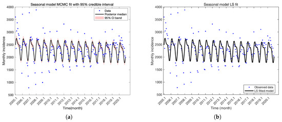
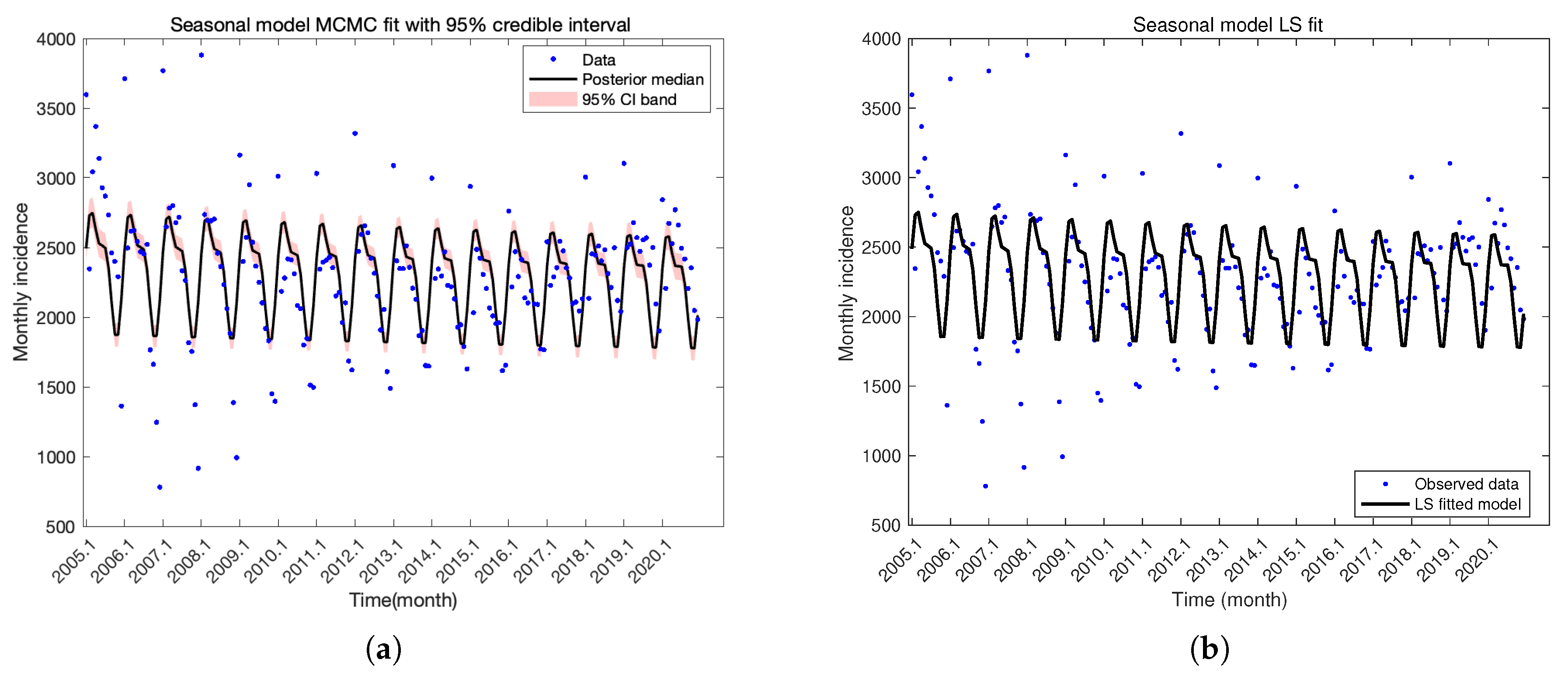
Similarly, we estimate the parameters of the seasonal system using the Markov Chain Monte Carlo (MCMC) method. The parameters to be estimated include ${\beta }_0$, ${\lambda }_0$, $a_1$, $a_2$, $a_3$, ${\varphi }_1$, ${\varphi }_2$, ${\varphi }_3$, $\tau$, $S\left(0\right)$, and $I\left(0\right)$. The MCMC procedure generates posterior distributions for these unknown parameters, from which the corresponding parameter confidence intervals can be obtained. The fitting results of the seasonal system are presented in Figure 12. The 95% posterior predictive band is relatively narrow, indicating that the parameter estimates obtained by the MCMC method are stable and well identified by the data. Although the observed data exhibit noticeable variability, the seasonal model successfully captures the main seasonal pattern of TB incidence. Compared with the averaged model, the seasonal model produces a much narrower credible band, suggesting that incorporating seasonal forcing significantly improves the model’s ability to describe the observed TB dynamics. The posterior means and 95% credible intervals of the estimated parameters for the seasonal system are summarized in Table 3.

Figure 12. MCMC fit of monthly TB incidence in Yunnan (2005–2020) based on the seasonal model with 95% credible interval.

Table 3. Posterior estimates of model parameters obtained by the MCMC method for the seasonal model.

Parameter	Mean	95% Credible Interval
${\beta }_0$	$3.8830\times {10}^{-10}$	$[3.8717\times {10}^{-10},3.9244\times {10}^{-10}]$
${\lambda }_0$	$2.7037\times {10}^{-8}$	$[2.6844\times {10}^{-8},2.7743\times {10}^{-8}]$
$a_1$	$5.9411\times {10}^{-1}$	$[5.9369\times {10}^{-1},5.9564\times {10}^{-1}]$
$a_2$	$1.6662\times {10}^{-1}$	$[1.6316\times {10}^{-1},1.6757\times {10}^{-1}]$
$a_3$	$3.9818\times {10}^{-1}$	$[3.9313\times {10}^{-1},4.1673\times {10}^{-1}]$
${\varphi }_1$	$-2.3208$	$[-2.3311,-2.2834]$
${\varphi }_2$	$3.2553$	$[3.2032,3.2695]$
${\varphi }_3$	$9.6900\times {10}^{-1}$	$[9.6119\times {10}^{-1},9.9768\times {10}^{-1}]$
$\tau$	$1.4599$	$[1.4046,1.4750]$
$S\left(0\right)$	$4.5727\times {10}^7$	$[4.5721\times {10}^7,4.5751\times {10}^7]$
$I\left(0\right)$	$8.8728\times {10}^4$	$[8.8428\times {10}^4,8.9829\times {10}^4]$

To evaluate the model performance quantitatively, we consider the following criteria.

(1) The Akaike information criterion ($AIC$) and its corrected version ($AI{C}_c$). When the number of observations is sufficiently large relative to the number of parameters, i.e., $K<N/40$, Akaike [37] introduced the statistic $AIC$ defined as

$$AIC=2K-2logL,$$

where K denotes the total number of free parameters in the model and L is the likelihood function. When the number of observations is relatively small compared with the number of parameters, i.e., $K>N/40$, Sugiura [38] proposed a corrected version of $AIC$, namely

$$AI{C}_c=AIC+{\displaystyle \frac{2K(K+1)}{N-K-1}},$$

where N denotes the number of observations. The model selection is to choose the model with the lowest $AI{C}_c$.

(2) The root mean square error ($RMSE$). The $RMSE$ is widely used to measure the accuracy of regression models [39]. It is defined as

$$RMSE=\sqrt{{\displaystyle \frac{1}{N}}\sum _{i=1}^N{(y_i-{\widehat{y}}_i)}^2},$$

where N denotes the sample size, and $y_i$ and ${\widehat{y}}_i$ represent the observed and predicted incidences at time i, respectively. A smaller $RMSE$ indicates that the model predictions are closer to the observed data, implying better predictive performance.

To further refine the parameter estimates, the posterior means obtained from the MCMC samples are used as the initial values for the least-squares optimization. The least-squares estimation is then performed separately for the averaged system and the periodic system. The parameter estimates of the averaged model obtained by the least-squares (LS) method are

$$\beta =1.2273\times {10}^{-9},\lambda =2.8556\times {10}^{-11},S\left(0\right)=2.3961\times {10}^7,I\left(0\right)=8.1275\times {10}^4.$$

The parameter estimates of the seasonal model obtained by the least-squares (LS) method are

$$\begin{array}{cc}\hfill {\beta }_0& =3.8793\times {10}^{-10},{\lambda }_0=2.7918\times {10}^{-8},a_1=5.7940\times {10}^{-1},\hfill \\ \hfill a_2& =1.5368\times {10}^{-1},a_3=4.1050\times {10}^{-1},{\varphi }_1=-2.3943,{\varphi }_2=3.3820,\hfill \\ \hfill {\varphi }_3& =8.2831\times {10}^{-1},\tau =1.4118,S\left(0\right)=4.5760\times {10}^7,I\left(0\right)=9.4712\times {10}^4.\hfill \end{array}$$

(31)

Based on the parameter estimates obtained by the least-squares (LS) method for the two models, the basic reproduction numbers of the averaged model and the seasonal model are

$$R_0\approx 1.785,{\mathcal{R}}_0\approx 0.564.$$

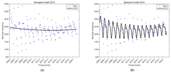
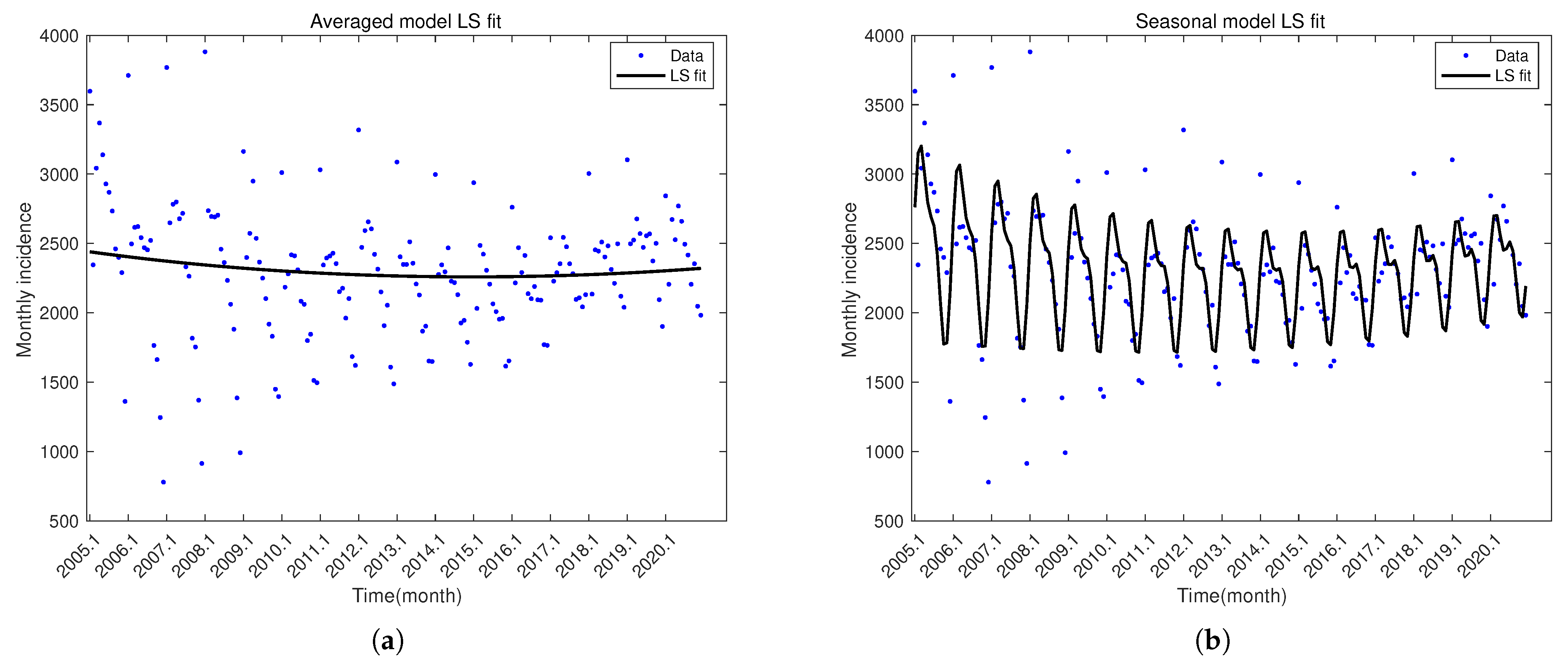
The corresponding fitting results are shown in Figure 13 and the resulting statistics are summarized in Table 4.

Figure 13. Comparison of model fitting results. (a) Averaged model fitting results. (b) Seasonal model fitting results.

Table 4. Summary of $AIC$, $AI{C}_c$, and $RMSE$ for the averaged model and the seasonal model.

Model	K	AIC	${\mathbf{AIC}}_{\mathit{c}}$	RMSE
Averaged model	4	2917.313	2917.527	472.198
Seasonal model	11	2825.724	2827.191	358.679

As shown in Table 4, the seasonal model yields smaller values of $AIC$, $AI{C}_c$, and $RMSE$ than the averaged model, indicating that the seasonal model provides a better fit to the data. When the parameters are estimated independently, the basic reproduction number of the averaged model is $R_0\approx 1.785$, whereas that of the seasonal model is ${\mathcal{R}}_0\approx 0.564$. This result suggests that, when seasonal transmission is ignored, the averaged model tends to compensate for the missing seasonal structure by increasing the constant transmission rate. Consequently, the averaged model may overestimate the transmission potential and the epidemic trend, whereas the seasonal model captures the temporal variability of transmission more realistically. These results highlight the importance of incorporating seasonal variation when modeling diseases with clear seasonal patterns.

As shown in Figure 13b, the fitted curve of the seasonal model exhibits clear peaks, secondary peaks, and troughs. To further illustrate the seasonal characteristics observed in the fitting results, we examine the actual TB incidence data. Specifically, for each year from 2005 to 2020, we identify the months corresponding to the largest and second-largest incidences, as well as the smallest and second-smallest incidences. The results are summarized in Table 5.

Table 5. Months corresponding to the two highest and two lowest TB incidences in Yunnan Province for each year.

Year	Maximum Incidence				Minimum Incidence
	Month	Max1	Month	Max2	Month	Min1	Month	Min2
2005	January	3597	April	3368	December	1362	November	2290
2006	January	3711	April	2622	December	780	November	1246
2007	January	3768	April	2799	December	915	November	1371
2008	January	3881	February	2736	December	992	November	1387
2009	January	3163	April	2949	December	1397	November	1450
2010	January	3011	April	2418	December	1496	November	1513
2011	January	3031	May	2430	December	1621	November	1685
2012	January	3318	April	2656	December	1488	November	1609
2013	January	3087	May	2512	December	1649	November	1653
2014	January	2997	May	2468	December	1629	November	1788
2015	January	2938	Mar	2486	November	1616	December	1654
2016	January	2761	Mar	2470	December	1766	November	1771
2017	May	2544	January	2541	November	2043	September	2097
2018	January	3004	May	2510	December	2040	November	2120
2019	January	3103	April	2677	December	1902	November	2095
2020	January	2843	May	2770	December	1983	November	2048

From Table 5, it can be observed that the trough and the second trough of TB incidence are mainly concentrated in November and December. This phenomenon may be associated with the relatively lower transmission intensity in late autumn and the time delay between infection, symptom development, and diagnosis. In contrast, the peak and the second peak of TB incidence are mainly concentrated in January and in the spring months (March–May) of each year. This seasonal pattern may be related to the climatic and social conditions in Yunnan Province. The relatively mild and humid climate in winter may create favorable conditions for the survival and transmission of Mycobacterium tuberculosis. During winter, lower temperatures and reduced ventilation tend to increase indoor crowding, which facilitates disease transmission. In addition, TB infection often has a certain incubation and diagnostic delay, so infections occurring in winter may be diagnosed and reported in the following spring. Moreover, the large-scale population movement associated with the Spring Festival may further increase contact opportunities and contribute to the rise in reported cases during this period. These epidemiological observations provide empirical support for incorporating seasonal forcing into the transmission rate in the proposed model.

4.4.3. Constrained Simulation Based on the Averaged Parameter Estimates

In Section 3.1, we showed that the seasonal model and the averaged model share the same basic reproduction number. To further investigate whether the endemic equilibrium of the averaged model can serve as a reliable proxy for the mean prevalence of the periodic oscillations, we perform a constrained numerical simulation in which the basic reproduction number is kept the same for the two models.

Case 1: parameters derived from the averaged model.

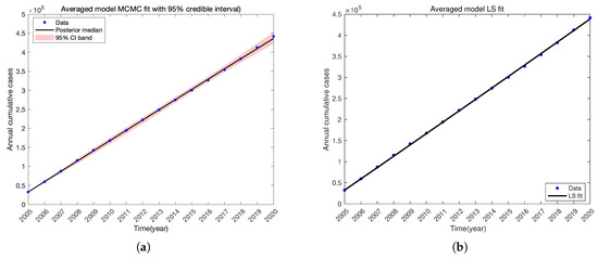
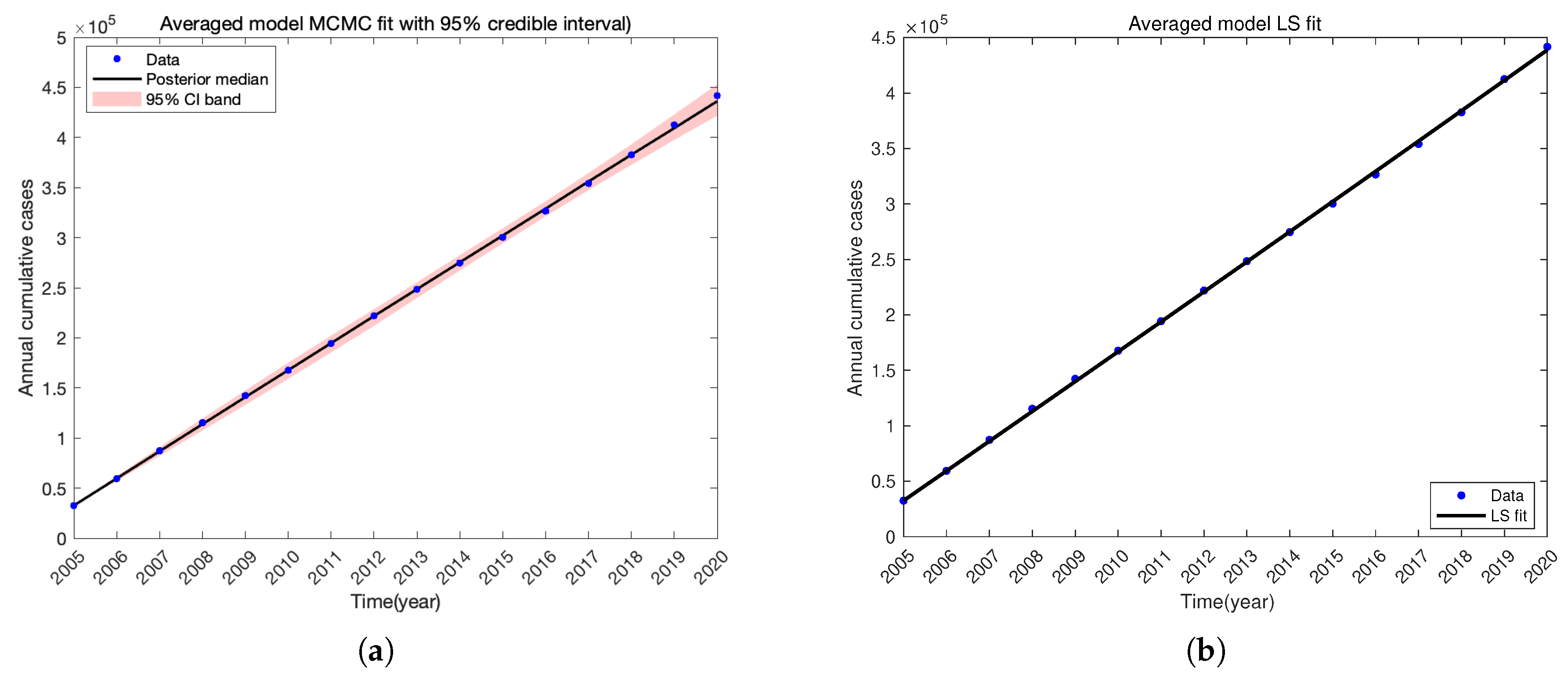
First, using the annual cumulative TB case data from 2005 to 2020, the parameter ranges are estimated via the Markov Chain Monte Carlo (MCMC) method, as shown in Figure 14a. The posterior means of the parameters $\tilde{\beta }$, $\tilde{\lambda }$, $S\left(0\right)$, and $I\left(0\right)$ are obtained, together with their corresponding 95% credible intervals in Table 6. Note that, since the numerical simulations are performed using annual cumulative data, the parameters $\tilde{\beta }$ and $\tilde{\lambda }$ correspond to the annual transmission rate and reinfection rate, respectively.

Figure 14. Comparison of model fitting results for the averaged model: (a) MCMC fit. (b) Least-squares (LS) fit.

Table 6. Posterior estimates of the averaged model parameters obtained by the MCMC method using annual cumulative data.

Parameter	Mean	95% Credible Interval
$\tilde{\beta }$	$8.7422\times {10}^{-9}$	$[7.2972\times {10}^{-9},9.8943\times {10}^{-9}]$
$\tilde{\lambda }$	$6.4056\times {10}^{-9}$	$[2.5416\times {10}^{-9},9.3653\times {10}^{-9}]$
$S\left(0\right)$	$3.4558\times {10}^7$	$[2.4928\times {10}^7,4.4524\times {10}^7]$
$I\left(0\right)$	$7.1597\times {10}^4$	$[6.1106\times {10}^4,8.1483\times {10}^4]$

Taking the posterior means as the initial values for the least-squares (LS) optimization, we further estimate the parameters $\tilde{\beta }$ and $\tilde{\lambda }$ of the averaged system. The corresponding fitting results are shown in Figure 14b.

The LS estimates are

$$\tilde{\beta }=8.6799\times {10}^{-9},\tilde{\lambda }=7.1015\times {10}^{-9}.$$

Based on these parameter estimates, the basic reproduction number of the averaged system is calculated as

$$R_0={\displaystyle \frac{\tilde{\beta }K}{\tilde{\alpha }+\tilde{b}}}\approx 1.0527.$$

Since $R_0>1$, the averaged system admits a positive endemic equilibrium given by

$$(S^{*},I^{*},R^{*})=(3.4580893690\times {10}^7,2.4836935937\times {10}^5,1.1345736950\times {10}^7).$$

Based on the conclusion that the two models share the same basic reproduction number, the estimated parameters $\tilde{\beta }$ and $\tilde{\lambda }$ are treated as fixed quantities in the seasonal model. Next, the monthly TB incidence data from 2005 to 2020 are used to simulate the seasonal model. Since the previous parameter estimation is based on annual cumulative data, the corresponding yearly quantities are converted into monthly data for the seasonal simulation. Let ${\beta }_0=\tilde{\beta }/12$, ${\lambda }_0=\tilde{\lambda }/12$, $b=\tilde{b}/12$, $\alpha =\tilde{\alpha }/12$.

The remaining parameters of the seasonal model are first estimated using the Markov Chain Monte Carlo (MCMC) method. The posterior means of the parameters are obtained together with their corresponding 95% credible intervals, as shown in Figure 15a and summarized in Table 7.

Figure 15. Comparison of model fitting results for the seasonal model: (a) MCMC fit. (b) Least-squares (LS) fit.

Table 7. Posterior estimates of the seasonal model parameters obtained by the MCMC method.

Parameter	Mean	95% Credible Interval
$a_1$	$8.8856\times {10}^{-2}$	$[8.1237\times {10}^{-3},1.9641\times {10}^{-1}]$
$a_2$	$1.1157\times {10}^{-1}$	$[8.0581\times {10}^{-2},1.4283\times {10}^{-1}]$
$a_3$	$4.0423\times {10}^{-1}$	$[1.7014\times {10}^{-1},4.9723\times {10}^{-1}]$
${\varphi }_1$	$-3.7497$	$[-5.3120,-1.7594]$
${\varphi }_2$	$1.1927$	$[-1.0004,3.3648]$
${\varphi }_3$	$2.6689$	$[1.2125,3.9323]$
$\tau$	$3.6102$	$[1.5649,5.7289]$
$S\left(0\right)$	$3.0487\times {10}^7$	$[2.8005\times {10}^7,3.2552\times {10}^7]$
$I\left(0\right)$	$7.5150\times {10}^4$	$[7.2370\times {10}^4,7.8303\times {10}^4]$

Taking the posterior means as the initial values for the least-squares (LS) optimization, we further estimate the parameters of the seasonal model. The corresponding fitting results are shown in Figure 15b. The LS estimates are

$$\begin{array}{cc}\hfill a_1& =2.9416\times {10}^{-2},a_2=1.1148\times {10}^{-1},a_3=5.0000\times {10}^{-1},{\varphi }_1=-3.9739,\hfill \\ \hfill {\varphi }_2& =1.2761,{\varphi }_3=2.7007,\tau =3.5322,S\left(0\right)=3.0781\times {10}^7,I\left(0\right)=7.4775\times {10}^4.\hfill \end{array}$$

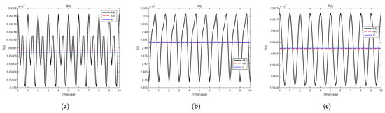
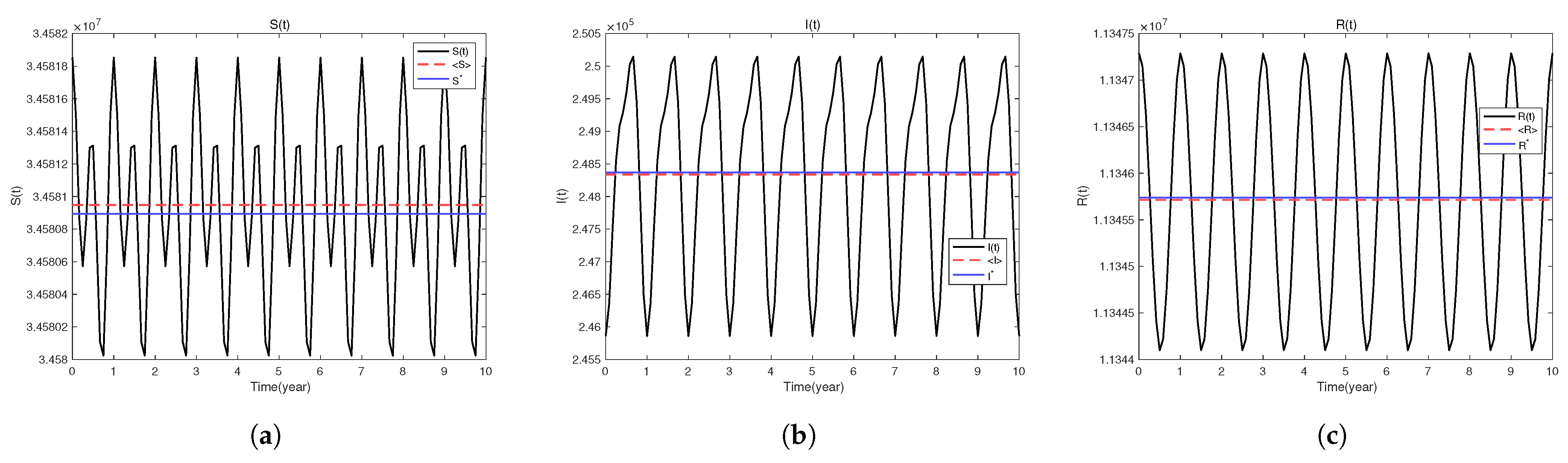
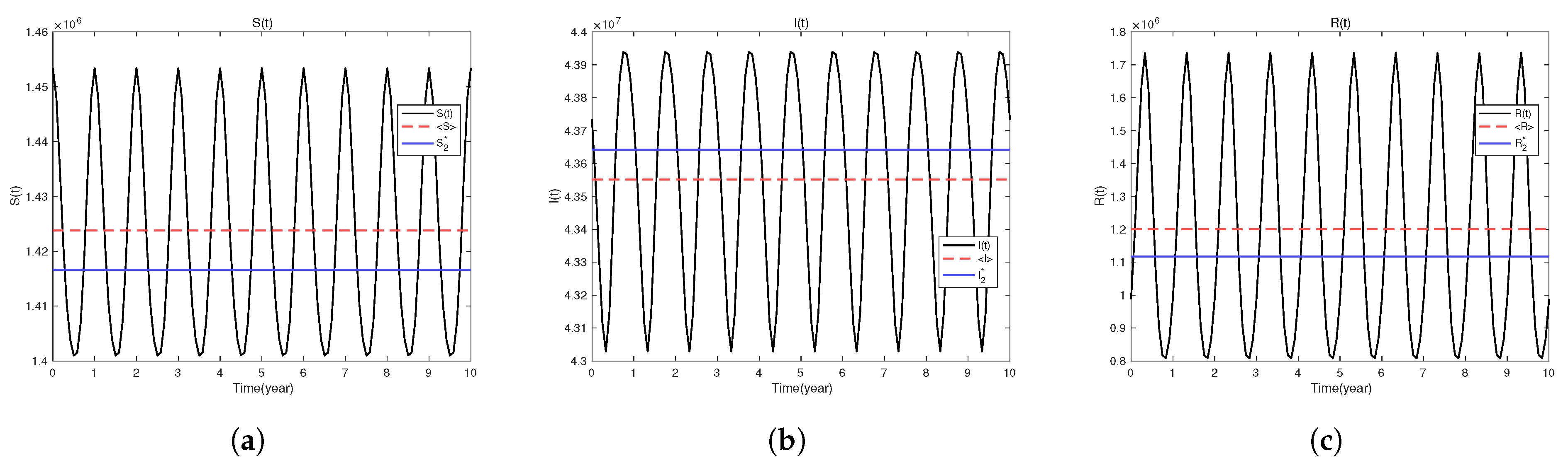
To further explore the long-term behavior of the models, numerical simulations are performed over a sufficiently long time horizon. After discarding the long transient dynamics, the trajectories during the last ten years near the steady state are plotted in Figure 16.

Figure 16. Trajectories of the periodic solution near the steady state for the seasonal model under the parameter setting of Case 1. After discarding the long transient phase, the last ten years of the trajectories are plotted. $(S^{*},I^{*},R^{*})$ denotes the endemic equilibrium of the corresponding averaged model. $⟨S⟩$, $⟨I⟩$, and $⟨R⟩$ denote the time-averaged values of $S\left(t\right)$, $I\left(t\right)$, and $R\left(t\right)$, respectively. (a) $S\left(t\right)$, (b) $I\left(t\right)$, and (c) $R\left(t\right)$.

Taking the infected population as an example, the mean value of $I\left(t\right)$ over the display period is used to characterize the average prevalence of the periodic oscillations. Specifically, the time average of $I\left(t\right)$ over one period $[0,\omega ]$ is defined by

$$⟨I⟩={\displaystyle \frac{1}{\omega }}{\int }_0^{\omega }I\left(t\right)dt,$$

where $\omega$ denotes the period of the seasonal forcing.

Since the numerical solution is obtained at discrete time points, the integral is approximated by the discrete average

$$⟨I⟩\approx {\displaystyle \frac{1}{N}}\sum _{k=1}^{N}I\left(t_k\right),$$

where $t_k$$(k=1,2,\dots ,N)$ are the sampled time points within the display period and N is the total number of samples. In the simulations, the state variables are recorded monthly, and therefore $N=10\times 12$ for a ten-year display period.

Using the same procedure, the time-averaged values $⟨S⟩$ and $⟨R⟩$ are computed in an analogous manner. The resulting numerical values are

$$⟨S⟩=3.4580948255\times {10}^7,⟨I⟩=2.4833831267\times {10}^5,⟨R⟩=1.1345713433\times {10}^7.$$

As shown in Figure 16, the dashed red lines denote the time-averaged values $⟨S⟩$, $⟨I⟩$, and $⟨R⟩$, while the solid blue lines represent the endemic equilibrium $(S^{*},I^{*},R^{*})$ of the averaged model. The figure suggests that the periodic trajectories oscillate around the endemic equilibrium of the averaged system.

To quantify the deviation between the time-averaged values of the periodic solution and the endemic equilibrium of the averaged model, we define the relative error

$${\eta }_X={\displaystyle \frac{|⟨X⟩-X^{*}|}{X^{*}}},X\in \{S,I,R\}.$$

The computed values are

$${\eta }_S=1.58\times {10}^{-6},{\eta }_I=1.25\times {10}^{-4},{\eta }_R=2.07\times {10}^{-6}.$$

(32)

which are all extremely small.

These numerical results indicate that, for the model considered in this section and under the current parameter settings, the endemic equilibrium of the averaged system provides a good approximation to the mean prevalence of the periodic oscillations.

Case 2: parameters derived from the seasonal model.

In Section 4.4.2, we obtained a set of parameters for the seasonal model by directly fitting the monthly TB incidence data from 2005 to 2020. The estimated parameters are listed in (31). Based on these estimates, the corresponding parameters of the averaged model can be determined, where the transmission rate and reinfection rate of the averaged system are taken as ${\beta }_0$ and ${\lambda }_0$, respectively. Substituting the parameters into the averaged model yields the positive endemic equilibria

$$\begin{array}{cc}\hfill (S_1^{*},I_1^{*},R_1^{*})& =(4.5657305587\times {10}^7,1.5661643014\times {10}^4,5.0203276956\times {10}^5),\hfill \\ \hfill (S_2^{*},I_2^{*},R_2^{*})& =(1.4166019808\times {10}^6,4.3641614697\times {10}^7,1.1167833227\times {10}^6).\hfill \end{array}$$

Similar to Case 1, the trajectories during the last ten years near the steady state for Case 2 are shown in Figure 17. The time-averaged values of the state variables are calculated as

$$⟨S⟩=1.4237700795\times {10}^6,⟨I⟩=4.3550955624\times {10}^7,⟨R⟩=1.2002742963\times {10}^6.$$

Figure 17. Trajectories of the periodic solution near the steady state for the seasonal model under the parameter setting of Case 2. After discarding the long transient phase, the last ten years of the trajectories are plotted. $(S_2^{*},I_2^{*},R_2^{*})$ denotes the endemic equilibrium of the corresponding averaged model. $⟨S⟩$, $⟨I⟩$, and $⟨R⟩$ denote the time-averaged values of $S\left(t\right)$, $I\left(t\right)$, and $R\left(t\right)$, respectively. (a) $S\left(t\right)$, (b) $I\left(t\right)$, and (c) $R\left(t\right)$.

To quantify the difference between the time-averaged values of the periodic solution and the endemic equilibrium $(S_2^{*},I_2^{*},R_2^{*})$ of the averaged system, the relative deviations are obtained as

$${\eta }_S=5.060065\times {10}^{-3},{\eta }_I=2.077354\times {10}^{-3},{\eta }_R=7.476023\times {10}^{-2}.$$

(33)

The relative deviations for the susceptible and infected populations are small (${\eta }_S\approx 0.5\%$ and ${\eta }_I\approx 0.2\%$), indicating that the endemic equilibrium of the averaged model still provides a reasonable approximation to the mean levels of $S\left(t\right)$ and $I\left(t\right)$ in the periodic system. However, the deviation for the recovered population is relatively larger (${\eta }_R\approx 7.5\%$), suggesting that the seasonal oscillations may have a stronger impact on the recovered class.

The results obtained in Case 1 and Case 2 reveal different approximation behaviors between the averaged model and the seasonal model. In Case 1, the relative deviations between the time-averaged values of the periodic solution and the endemic equilibrium of the averaged system are extremely small, indicating that the endemic equilibrium of the averaged model provides an excellent approximation to the mean prevalence of the periodic oscillations. In contrast, in Case 2, although the deviations for the susceptible and infected populations remain relatively small, the deviation for the recovered population becomes noticeably larger. These results indicate that the endemic equilibrium of the averaged system can approximate the mean prevalence of the periodic solution under certain parameter conditions, but this approximation is not guaranteed in general.

5. Discussion

In this paper, we studied a tuberculosis transmission model with reinfection based on the SIRI framework, with a particular focus on the relationship between the averaged system and the periodic system. We showed that the averaged system and the seasonal (periodic) system share the same basic reproduction number, indicating that $R_0$ can serve as an important threshold quantity in the analysis of the disease dynamics. The coincidence of the basic reproduction number is not accidental; rather, it is a structural consequence of the one-dimensional infected subsystem near the disease-free state. As shown in Equation (3), the infected subsystem takes the form

$$\dot{I}\left(t\right)=[F\left(t\right)-V\left(t\right)]I\left(t\right),$$

where $F\left(t\right)$ represents the rate of new infections and $V\left(t\right)$ denotes the rate at which infected individuals leave the infected class. Both $F\left(t\right)$ and $V\left(t\right)$ are one-dimensional $\omega$-periodic functions. By the analysis in Section 2.1, the evolution operator can be written as

$$W(t,s,\xi )=exp\left({\int }_s^t\left[-V\left(\tau \right)+{\displaystyle \frac{F\left(\tau \right)}{\xi }}\right]d\tau \right).$$

Since ${\mathcal{R}}_0$ is the unique solution of $\rho \left(W(\omega ,0,{\mathcal{R}}_0)\right)=1$, it follows that

$${\int }_0^{\omega }\left[-V\left(\tau \right)+{\displaystyle \frac{F\left(\tau \right)}{{\mathcal{R}}_0}}\right]d\tau =0.$$

Define the time averages of $F\left(t\right)$ and $V\left(t\right)$ over one period $\omega$ by

$$⟨F⟩={\displaystyle \frac{1}{\omega }}{\int }_0^{\omega }F\left(t\right)dt,⟨V⟩={\displaystyle \frac{1}{\omega }}{\int }_0^{\omega }V\left(t\right)dt.$$

Then the basic reproduction number can be written as

$${\mathcal{R}}_0={\displaystyle \frac{⟨F⟩}{⟨V⟩}}.$$

The periodic system constructed in this paper is precisely a special case of it. In contrast, for multi-dimensional infected subsystems the threshold generally cannot be reduced to a simple ratio of time averages.

Moreover, we analyzed the threshold dynamics of the seasonal model and investigated the dynamical properties of the averaged system. In particular, the existence of backward bifurcation was demonstrated, implying that tuberculosis may persist even when the basic reproduction number is less than one. The existence and stability of equilibrium points were examined in detail, with special attention given to stability at the critical threshold value ($R_0=1$). These results highlight how transmission and reinfection jointly determine the disease burden and the equilibrium structure.

Numerical simulations are performed using the monthly tuberculosis incidence data in Yunnan Province, China, from 2005 to 2020. Sensitivity analysis of the basic reproduction number $R_0$ shows that reducing the transmission rate or increasing the recovery rate would be the most effective strategies for controlling disease transmission. Using the same dataset, all parameters of the averaged model and the seasonal model are estimated and compared. The seasonal model yields smaller values of $AIC$, $AI{C}_c$, and $RMSE$ than the averaged model, indicating a better fitting performance. The numerical simulations suggest that the averaged model may overestimate the transmission potential of the disease. Finally, to investigate whether the endemic equilibrium of the averaged model can serve as a reasonable approximation to the mean prevalence of periodic oscillations under the same basic reproduction number, a constrained numerical simulation is performed. The results show that the endemic equilibrium of the averaged system can approximate the mean prevalence of the periodic solution under certain parameter conditions, but this approximation is not guaranteed in general.

From an applied perspective, numerical simulations based on tuberculosis data from Yunnan Province indicate that the averaged system effectively captures the fundamental transmission mechanisms and threshold behavior of tuberculosis, whereas the periodic system successfully reproduces the seasonal oscillations and short-term fluctuations observed in the reported data. Overall, our results provide valuable mathematical tools and theoretical insights for understanding tuberculosis transmission dynamics in high-burden regions and for informing disease control strategies.

References

- Kermack, W.O.; McKendrick, A.G. A contribution to the mathematical theory of epidemics. Proc. R. Soc. Lond. A 1927, 115, 700–721. [Google Scholar] [CrossRef] [Scilit]
- Kermack, W.O.; McKendrick, A.G. Contributions to the mathematical theory of epidemics. II. The problem of endemicity. Proc. R. Soc. Lond. A 1932, 138, 55–83. [Google Scholar] [CrossRef] [Scilit]
- Kermack, W.O.; McKendrick, A.G. Contributions to the mathematical theory of epidemics. III. Further studies of the problem of endemicity. Proc. R. Soc. Lond. A 1933, 141, 94–112. [Google Scholar] [CrossRef] [Scilit]
- Gomes, G.M.; White, L.J.; Medley, G.F. Infection, reinfection, and vaccination under suboptimal immune protection. J. Theor. Biol. 2004, 228, 539–549. [Google Scholar] [CrossRef] [Scilit]
- Song, L.P.; Jin, Z.; Sun, G.Q. Reinfection induced disease in a spatial SIRI model. J. Biol. Phys. 2011, 37, 133–140. [Google Scholar] [CrossRef] [Scilit]
- Xu, Z.; Xu, Y.; Huang, Y. Traveling waves for a spatial SIRI epidemic model. Taiwan. J. Math. 2019, 23, 1435–1460. [Google Scholar] [CrossRef] [Scilit]
- Verver, S.; Warren, R.M.; Beyers, N.; Richardson, M.; van der Spuy, G.D.; Borgdorff, M.W.; Enarson, D.A.; Behr, M.A.; van Helden, P.D. Rate of reinfection tuberculosis after successful treatment is higher than rate of new tuberculosis. Am. J. Respir. Crit. Care Med. 2005, 171, 1430–1435. [Google Scholar] [CrossRef] [Scilit]
- Mithunage, C.T.; Denning, D.W. Timing of recurrence after treatment of pulmonary tuberculosis. IJTLD Open 2024, 1, 456–465. [Google Scholar] [CrossRef] [Scilit]
- Shen, G.; Xue, Z.; Shen, X.; Sun, B.; Gui, X.; Shen, M.; Mei, J.; Gao, Q. Recurrent tuberculosis and exogenous reinfection, Shanghai, China. Emerg. Infect. Dis. 2006, 12, 1776–1778. [Google Scholar] [CrossRef] [Scilit]
- Uys, P.W.; van Helden, P.D.; Hargrove, J.W. Tuberculosis reinfection rate as a proportion of total infection rate correlates with the logarithm of the incidence rate: A mathematical model. J. R. Soc. Interface 2009, 6, 11–15. [Google Scholar] [CrossRef] [Scilit]
- Vega, V.; Rodríguez, S.; van der Stuyft, P.; Seas, C.; Otero, L. Recurrent tuberculosis: A systematic review and meta-analysis of the incidence rates and the proportions of relapses and reinfections. Thorax 2021, 76, 494–502. [Google Scholar] [CrossRef] [Scilit] [PubMed]
- Aldila, D. Change in stability direction induced by temporal interventions: A case study of a tuberculosis transmission model with relapse and reinfection. Front. Appl. Math. Stat. 2025, 11, 1541981. [Google Scholar] [CrossRef] [Scilit]
- Schaaf, H.S.; Nel, E.D.; Beyers, N.; Gie, R.P.; Scott, F.; Donald, P.R. A decade of experience with Mycobacterium tuberculosis culture from children: A seasonal influence of childhood tuberculosis. Tuberc. Lung Dis. 1996, 77, 43–46. [Google Scholar] [CrossRef] [Scilit]
- Douglas, A.S.; Strachan, D.P.; Maxwell, J.D. Seasonality of tuberculosis: The reverse of other respiratory disease in the UK. Thorax 1996, 51, 944–946. [Google Scholar] [CrossRef] [Scilit] [PubMed]
- Leung, C.C.; Yew, W.W.; Chan, T.Y.K.; Tam, C.M.; Chan, C.Y.; Chan, C.K.; Tang, N.; Chang, K.C.; Law, W.S. Seasonal pattern of tuberculosis in Hong Kong. Int. J. Epidemiol. 2005, 34, 924–930. [Google Scholar] [CrossRef] [Scilit]
- Rios, M.; Garcia, J.M.; Sanchez, J.A.; Perez, D. A statistical analysis of the seasonality in pulmonary tuberculosis. Eur. J. Epidemiol. 2000, 16, 483–488. [Google Scholar] [CrossRef] [Scilit] [PubMed]
- Nagayama, N.; Ohmori, M. Seasonality in various forms of tuberculosis. Int. J. Tuberc. Lung Dis. 2006, 10, 1117–1122. [Google Scholar]
- Kirolos, A.; Thindwa, D.; Khundi, M.; Burke, R.M.; Henrion, M.Y.; Nakamura, I.; Divala, T.H.; Nliwasa, M.; Corbett, E.L.; MacPherson, P. Tuberculosis case notifications in Malawi have strong seasonal and weather-related trends. Sci. Rep. 2021, 11, 4621. [Google Scholar] [CrossRef] [Scilit]
- Taylan, M.; Dogru, S.; Sezgi, C.; Yılmaz, S. Epidemiological trends and seasonal dynamics of tuberculosis in Southeastern Turkey. Niger. J. Clin. Pract. 2023, 26, 928–933. [Google Scholar] [CrossRef] [Scilit]
- Xue, L.; Jing, S.; Wang, H. Evaluating strategies for tuberculosis to achieve the goals of WHO in China: A seasonal age-structured model study. Bull. Math. Biol. 2022, 84, 61. [Google Scholar] [CrossRef] [Scilit]
- Liu, L.; Zhao, X.-Q.; Zhou, Y. A tuberculosis model with seasonality. Bull. Math. Biol. 2010, 72, 931–952. [Google Scholar] [CrossRef] [Scilit]
- Bowong, S.; Kurths, J. Modeling and analysis of the transmission dynamics of tuberculosis without and with seasonality. Nonlinear Dyn. 2012, 67, 2027–2051. [Google Scholar] [CrossRef] [Scilit]
- Xue, L.; Jing, S.; Wang, H. Dynamics and optimal control for tuberculosis transmission via a data-validated periodic model. Infect. Dis. Model. 2025, in press. [Google Scholar]
- Pan, Y.; Zhou, J.; Qiu, Y.; Chen, J.; Yang, Y.; Wu, W.; Cheng, Y.; Xu, L. Comparison of results of two surveys of underreporting of pulmonary tuberculosis in county-level medical institutions in Yunnan. Dis. Surveill. 2023, 38, 299–303. [Google Scholar]
- Chen, J.; Qiu, Y.; Yang, R.; Li, L.; Hou, J.; Lu, K.; Xu, L. The characteristics of spatial-temporal distribution and cluster of tuberculosis in Yunnan Province, China, 2005–2018. BMC Public Health 2019, 19, 1715. [Google Scholar] [CrossRef] [Scilit]
- Chen, J.; Qiu, Y.; Wu, W.; Yang, R.; Li, L.; Yang, Y.; Yang, X.; Xu, L. Trends and projection of the incidence of active pulmonary tuberculosis in southwestern China: Age-period-cohort analysis. JMIR Public Health Surveill. 2023, 9, e48015. [Google Scholar] [CrossRef] [Scilit] [PubMed]
- Lozano-Ochoa, E.; Camacho, J.F.; Vargas-De-León, C. Qualitative stability analysis of an obesity epidemic model with social contagion. Discrete Dyn. Nat. Soc. 2017, 2017, 1084769. [Google Scholar] [CrossRef] [Scilit]
- Wang, W.; Zhao, X.-Q. Threshold dynamics for compartmental epidemic models in periodic environments. J. Dyn. Diff. Equat. 2008, 20, 699–717. [Google Scholar] [CrossRef] [Scilit]
- Zhao, X.-Q. Dynamical Systems in Population Biology, 2nd ed.; Springer: Cham, Switzerland, 2017. [Google Scholar]
- Zhang, Z.; Ding, T.; Huang, W.; Dong, Z. Qualitative Theory of Differential Equations; Translations of Mathematical Monographs; American Mathematical Society: Providence, RI, USA, 1992; Volume 101. [Google Scholar]
- Ma, Z.; Zhou, Y. Qualitative and Stability Methods of Ordinary Differential Equations; Science Press: Beijing, China, 2001. [Google Scholar]
- Yang, Y.; Liu, L.; Chen, J.; Li, L.; Qiu, Y.; Wu, W.; Xu, L. Predicting the incidence of rifampicin-resistant tuberculosis in Yunnan, China: A seasonal time series analysis based on routine surveillance data. BMC Infect. Dis. 2024, 24, 835. [Google Scholar] [CrossRef] [Scilit]
- Chinese Center for Disease Control and Prevention. Public Health Science Data Center. Available online: https://www.phsciencedata.cn/Share/edtShareNew.jsp?id=39204 (accessed on 10 December 2025).
- National Bureau of Statistics of China. China Statistical Yearbook 2006–2021; China Statistics Press: Beijing, China, 2021. [Google Scholar]
- Wu, Z.Y.; Yang, J.Y. Study on parameter identifiability of an age-structured tuberculosis model with relapse. Acta Math. Sci. Ser. A 2025, 45, 269–278. [Google Scholar]
- Chitnis, N.; Hyman, J.M.; Cushing, J.M. Determining important parameters in the spread of malaria through the sensitivity analysis of a mathematical model. Bull. Math. Biol. 2008, 70, 1272–1296. [Google Scholar] [CrossRef] [Scilit] [PubMed]
- Akaike, H. A new look at the statistical model identification. IEEE Trans. Autom. Control 1974, 19, 716–723. [Google Scholar] [CrossRef] [Scilit]
- Sugiura, N. Further analysis of the data by Akaike’s information criterion and the finite corrections. Commun. Stat. Theory Methods 1978, 7, 13–26. [Google Scholar] [CrossRef] [Scilit]
- Yang, W.; Zhang, D.; Peng, L.; Zhuge, C.; Hong, L. Rational evaluation of various epidemic models based on the COVID-19 data of China. Epidemics 2021, 37, 100501. [Google Scholar] [CrossRef] [Scilit]
Disclaimer/Publisher’s Note: The statements, opinions and data contained in all publications are solely those of the individual author(s) and contributor(s) and not of MDPI and/or the editor(s). MDPI and/or the editor(s) disclaim responsibility for any injury to people or property resulting from any ideas, methods, instructions or products referred to in the content. |
© 2026 by the authors. Licensee MDPI, Basel, Switzerland. This article is an open access article distributed under the terms and conditions of the Creative Commons Attribution (CC BY) license.