


Abstract
To meet the real-time computational requirements of active suspension control systems, this study shifts from complex microscopic physical equations to a direct nonlinear functional mapping between the relative motion states (displacement and velocity) and the output force of air springs. This approach aims to preserve critical nonlinear hysteresis characteristics while significantly reducing the computational overhead. A progressive modeling strategy is implemented to characterize these complex behaviors. Initially, polynomial fitting is employed to identify key input features; however, its limited capacity to capture intricate nonlinearities necessitates more advanced methods. Subsequently, standard Feedforward Neural Networks (FNNs) are explored for their nonlinear mapping capabilities, yet their inherent “black-box” nature often leads to convergence difficulties and restricted generalization. To address these issues, a Physics-Informed Neural Network (PINN) architecture is introduced, embedding physical governing equations as regularization constraints within the loss function to integrate data-driven flexibility with mathematical rigor. Recognizing that conventional PINNs often encounter convergence challenges due to conflicts between PDE constraints and data-driven loss terms, this research develops a Physics-Embedded Hierarchical Network (PEHN). By deriving specialized PDE constraints tailored to air spring dynamics and designing a hierarchical architecture aligned with these physical requirements, the PEHN effectively balances physical priors with experimental data. Experimental results demonstrate that, compared to the baseline models, the proposed PEHN exhibits stronger stability and superior accuracy in capturing the complex nonlinearities of air spring dynamics.
MSC:
68T05
1. Introduction
As a critical component of modern automotive suspension systems, air springs play a pivotal role in enhancing ride comfort and handling stability, owing to their superior vibration isolation, adjustable stiffness, and height control capabilities. In contrast to traditional coil springs, the mechanical properties of air springs exhibit significant nonlinearity. This unique mechanical behavior affords them greater dynamic adaptability within active or semi-active suspension systems, allowing for adjustments based on varying driving conditions to optimize overall vehicle performance [1].
In the development of active suspension control systems, establishing a high-precision dynamic model of the air spring is a fundamental prerequisite for achieving closed-loop control [2]. Recent research into control strategies has frequently employed parametric modeling based on macroscopic characteristics. By establishing a functional mapping between the output force and the relative motion parameters of the sprung and unsprung masses [3], this method effectively characterizes the system’s dynamic properties. Compared with first-principles physical modeling derived from gas equations of state, this data-driven parametric method accurately captures nonlinear hysteresis and dynamic stiffness variations [4], while simultaneously avoiding the heavy computational burden associated with complex fluid–structure interaction modeling.
Relevant research has been conducted on the characteristic modeling of air springs. Wu et al. [5] integrated thermodynamics and structural dynamics to develop a general model for dual-chamber air springs, elucidating the physical mechanisms behind stiffness and damping terms, particularly their frequency dependence. To address simulation complexities, Li et al. [6] employed fluid–structure interaction (FSI) modeling, revealing a significant performance asymmetry where axial compression proves more sensitive than tension due to radial load coupling. Further, Zhu et al. [7] proposed a high-fidelity model incorporating variable Berg friction and fractional derivatives. Unlike traditional linear models, their approach excels under large-amplitude excitations by capturing nonlinear elasticity and asymmetric hysteresis. Similarly, Chen et al. [8] derived the structural parameter models of the air spring using a geometrical method and introduced a new pressure factor to better characterize its mechanical behavior.
Although the aforementioned studies have significantly enhanced the physical fidelity and prediction accuracy of air spring models by incorporating thermodynamics, fluid–structure interaction, and fractional derivative theories, these models generally suffer from complex mathematical structures, challenging parameter identification, and high computational resource consumption. From the perspective of practical control strategy application, control systems prioritize the model’s real-time computational efficiency and feasibility within the vehicle’s onboard controller.
Consequently, instead of relying solely on complex microscopic physical equations, this study directly establishes a nonlinear functional mapping between the relative motion states (displacement and velocity) of the sprung and unsprung masses and the air spring output force. This approach aims to preserve the system’s critical nonlinear hysteresis characteristics while significantly reducing the computational burden, thereby meeting the real-time requirements of active suspension control systems.
In this study, a progressive modeling strategy is implemented to characterize the nonlinear behavior of air springs. Initially, polynomial fitting is employed not only to provide a preliminary representation but also to identify critical input features from the dataset [9]. However, due to the limited capacity of polynomials in capturing intricate nonlinearities, standard Feedforward Neural Networks (FNNs) [10] are subsequently explored. Although FNNs excel at nonlinear mapping, their inherent “black-box” nature often leads to convergence difficulties and restricted generalization. To overcome these limitations, a Physics-Informed Neural Network (PINN) [11] architecture is introduced. As a transformative paradigm in scientific computing, PINN has demonstrated exceptional robustness in solving complex nonlinear problems, even when faced with sparse or noisy data [12]. By embedding physical governing equations into the loss function as regularization constraints, the PINN model seamlessly integrates the flexibility of data-driven methods with the mathematical rigorousness of physical laws.
While Physics-Informed Neural Networks (PINNs) offer significant advantages, conventional PINN architectures often encounter convergence challenges [13]. Specifically, conflicts between PDE constraints and data-driven loss terms can arise, preventing the network from converging to the global optimum [14]. To address these limitations, this study refines the standard PINN framework by developing a Physics-Embedded Hierarchical Network (PEHN). By deriving specialized PDE constraints tailored to the dynamic characteristics of air springs and designing a hierarchical neural architecture aligned with these physical requirements [15], the PEHN effectively balances physical priors with experimental data. This approach ensures more robust convergence and a superior ability to capture complex behaviors, including nonlinearities, hysteresis effects, and dynamic stiffness variations. The resulting high-fidelity model not only accurately characterizes instantaneous mechanical responses but also provides a critical foundation for advanced suspension control strategies [16], such as Model Predictive Control (MPC), to enhance vehicle adaptability under dynamic loads. The overall research technical roadmap is illustrated in Figure 1, which details the evolutionary process from data acquisition to the proposed PEHN model.
Figure 1.
Proposed Technical Roadmap of Air Spring Nonlinear Modeling.
The main innovations of this paper are summarized as follows: (1) Control-Oriented Characteristic Analysis: The external characteristics of the air spring are investigated from the perspective of control requirements. By utilizing the relative motion parameters between the sprung and unsprung masses as inputs, the output force of the air spring is directly obtained. (2) High-Precision Surrogate Modeling: A Feedforward Neural Network (FNN) surrogate model is developed. This approach leverages the powerful nonlinear expression capability of neural networks to achieve higher precision in air spring modeling compared to traditional methods. (3) Physics-Informed Neural Network Integration: A neural network model based on physical information is constructed. This integration accelerates the network’s convergence speed and guides the model to converge in a direction consistent with physical laws, thereby significantly enhancing both prediction accuracy and generalization capability.
2. Experimental Study on External Characteristics of Air Springs
This research emphasizes the characterization of a system’s physical behavior through experimental data. High-quality experimental datasets regarding the external characteristics of air springs not only record mechanical responses under diverse operating conditions but also systematically reveal the inherent evolution of damping and stiffness variations [17]. Such data provides a robust foundation for establishing accurate mappings from operating states to mechanical performance. By leveraging these comprehensive datasets, the implemented modeling techniques—ranging from polynomial fitting for feature identification to neural networks for complex nonlinear capturing—can achieve high predictive accuracy while maintaining consistency with physical trends.
2.1. Preliminary Modeling of Air Springs
Assuming the air inside the air spring behaves as an ideal gas and the internal pressure is uniformly distributed, the external force of the air spring can be expressed as:
where denotes the effective area of the air spring, represents the pressure within the working volume, and is the atmospheric pressure.
Air springs are suspension elements that use compressed air as an elastic medium, extensively used in automotive and high-speed railway applications. Operating on the principle of gas compressibility, the internal air generates an elastic force through compression or expansion under load. Therefore, the ideal gas polytropic equation is employed to describe the dynamic behavior of the air spring [18]:
where denotes the gas pressure and denotes the gas volume, is the polytropic exponent, determined by heat exchange conditions. Specifically, corresponds to an isothermal process (characterized by slow change and sufficient heat exchange), while corresponds to an adiabatic process (characterized by rapid change and no heat exchange). For other conditions, the value of lies between 1 and 1.4.
The mechanical characteristics of an air spring are inherently nonlinear, and the evolution of its internal gas state is essentially the result of the coupling between geometric deformation and thermodynamic processes. Specifically, the effective volume varies nonlinearly with the relative displacement , while the relative velocity determines the rate of gas compression and expansion, thereby affecting the heat transfer process, the polytropic index , and the transient evolution of internal pressure. Therefore, under dynamic operating conditions, both the working volume and the internal pressure should be expressed as functions of displacement and velocity, namely and , so as to more accurately describe the mechanical response of the air spring [19].
Based on the aforementioned mechanism, it is necessary to establish a multi-physical quantity synchronous data acquisition system during the air spring external characteristic test. This system performs real-time measurement of key state variables during operation, including relative displacement , relative velocity , and internal pressure . Furthermore, given that thermal effects during gas compression and expansion are non-negligible under actual working conditions, the real-time gas temperature within the chamber must be synchronously monitored. This allows for the correction of gas state deviations caused by temperature changes during the modeling process, thereby enhancing the physical consistency and reliability of the experimental data.
Simultaneously, according to the ideal gas polytropic equation, differences in state variables at the initial moment will affect the state of the entire model, namely the following:
where represents the gas pressure at the initial state, and represents the initial volume of the gas within the air spring. The thermodynamic state of the system at the initial moment constitutes a critical boundary condition for the model. Specifically, the initial pressure and initial volume jointly determine the static equilibrium position and the fundamental stiffness characteristics of the air spring. Different initial states correspond to distinct stiffness evolution paths, thereby forming a family of mutually distinguishable stiffness curves. Therefore, during the testing process, the initial state parameters for each operating condition must be precisely calibrated and recorded. This ensures the accurate differentiation and unified modeling of various load levels and installation height conditions.
2.2. Test Rig Setup and Load Case Design
Guided by the aforementioned theoretical analysis and data acquisition requirements, a comprehensive experimental platform for characterizing air springs was established. This platform integrates mechanical excitation, pneumatic regulation, and high-frequency data acquisition capabilities, designed to precisely reproduce and observe the dynamic response of air springs under various operating conditions. The schematic diagram illustrating the overall control architecture and signal flow of the test rig is presented in Figure 2. As depicted, the testing system is primarily composed of three subsystems: the mechanical loading and execution unit, the pneumatic supply and regulation unit, and the real-time control and data acquisition unit (based on dSPACE). The specific hardware configurations and functions of these key subsystems are detailed as follows:
Figure 2.
Schematic Diagram of the Testing Process for the External Characteristics of Air Springs.
MTS850 Damper Test System (MTS Systems Corporation, Eden Prairie, MN, USA): To accurately investigate the mechanical properties of air springs under actual operating environments, this system is employed to apply preset loading excitations (including various typical input profiles) to the test specimen. During the loading process, integrated high-precision displacement sensors and velocity calculation modules capture the dynamic displacement response and velocity variation signals in real-time. Simultaneously, a force sensor located at the loading end synchronously acquires the instantaneous reaction force generated by the excitation. Through a multi-channel data acquisition system, the synchronized recording of displacement, velocity, and force signals is achieved, thereby obtaining the authentic dynamic response characteristics of the air spring under different loading conditions.
Air Spring: The specimen selected for this test is a double-chamber membrane air spring. Its design features a variable volume mechanism controlled by a solenoid valve. Specifically, when the solenoid valve is de-energized (normally open mode), the main and auxiliary chambers are connected, resulting in a total internal volume of . In this state, the air spring exhibits low stiffness, corresponding to the vehicle’s Comfort Mode. Conversely, when the solenoid valve is energized, the valve port closes, isolating the passage between the two chambers. Consequently, the effective working volume is reduced to . In this state, the air spring exhibits high stiffness, corresponding to the Sport Mode. Therefore, this experimental setup facilitates the acquisition of characteristic data for the air spring under two distinct initial volume configurations.
dSPACE MicroAutoBox III (dSPACE Group SE & Co. KG, Paderborn, Germany): The dSPACE MicroAutoBox III is a high-performance real-time control unit extensively utilized in Rapid Control Prototyping (RCP) and the testing of complex mechatronic systems. Serving as the core controller within this experimental platform, it is responsible for the centralized management and coordinated control of the entire test rig. Specifically, it generates precise excitation commands for the actuators based on preset operating conditions, ensuring that the dynamic characteristics of the mechanical loading process strictly adhere to experimental requirements. Simultaneously, through real-time closed-loop monitoring of the internal pressure within the air tank and air spring, it precisely regulates the solenoid valves and pneumatic supply equipment. This achieves both steady-state pressure maintenance and dynamic response regulation, thereby guaranteeing the stability and consistency of the system’s operational state.
Beyond its core control capabilities, the MicroAutoBox III features robust multi-channel high-speed data acquisition functions, enabling the real-time capture, processing, and synchronized recording of key sensor signals such as pressure, displacement, and load, thus providing a reliable basis for subsequent data analysis. Additionally, the controller integrates comprehensive safety monitoring logic, capable of immediately triggering protective measures, such as emergency stops or pressure relief, upon detecting system anomalies to prevent equipment damage or safety incidents. In summary, the MicroAutoBox III deeply integrates control decision-making, signal coordination, and data management functions within this system, serving as the pivotal equipment for achieving high-precision air spring characterization tests.
dSPACE RapidPro SC Unit (dSPACE Group SE & Co. KG, Paderborn, Germany): The dSPACE RapidPro SC Unit is a specialized signal conditioning and power stage unit within the dSPACE modular platform. It possesses robust signal processing capabilities, enabling high-precision amplification, filtering, isolation, and excitation supply for sensor signals, as well as interface matching and power adaptation for actuator drive signals. Designed to operate seamlessly with the MicroAutoBox III, it establishes a high-precision, low-noise, and stable signal link for real-time control systems. In this experimental platform, the RapidPro unit primarily functions as the physical layer interface: it is responsible for level shifting or power amplification of the logic signals originating from the core controller. This provides compatible input interfaces for solenoid valves, pneumatic components, and actuators, thereby ensuring the precision and responsiveness of the actuation system.
Pressure Sensors: Pressure sensors in this system are primarily responsible for full-process pneumatic monitoring. During the preparation and inflation phase, these sensors perform real-time closed-loop monitoring of the internal pressure within both the air spring and the reservoir, ensuring that the system precisely and stably reaches the target pressure settings. Throughout the dynamic testing phase, the sensors continuously acquire transient pressure response data from the air spring. This function serves a dual purpose: it allows for real-time monitoring to detect if pressure fluctuations deviate from the normal operating range (preventing over-pressure or under-pressure anomalies), and it records essential experimental data to support subsequent mechanical characteristic analysis and performance evaluation.
Temperature Sensors: Given that temperature variations affect the polytropic exponent of the gas and thus alter the mechanical properties of the air spring, the system is equipped with temperature sensors to monitor the internal gas temperature in real time. This measurement helps ensure data reliability by supporting the accurate acquisition of key thermodynamic parameters during testing and providing a physical basis for the subsequent correction of thermal effects.
Pneumatic Valves: During the testing process, sensors are installed on the external pneumatic circuit for parameter measurement. To minimize the influence of the external circuit’s volume on the effective working volume of the air spring, pneumatic valves (cutoff valves) are strategically positioned within the circuit. These valves are employed to reliably isolate the air spring from the upstream air supply (air reservoir) during measurement phases. This isolation effectively eliminates the interference of additional gas volume (dead volume) on the experimental results, thereby ensuring the physical fidelity of the test data.
Air Reservoir: The air reservoir plays a critical role in the air spring system, functioning as both a pressure stabilizer and a buffer. Firstly, acting as an intermediate energy storage element, it provides a sufficient and stable supply of compressed air to the air spring, effectively isolating the test object from pressure fluctuations originating from the upstream source (e.g., the compressor). Secondly, during inflation and deflation regulation, the reservoir buffers airflow variations, significantly dampening pressure pulsations and enhancing the system’s dynamic stability and control precision. Furthermore, the stored pneumatic energy facilitates the rapid establishment of the air spring’s initial operating pressure, ensuring the efficient and reliable execution of test conditions.
The design of the test conditions aims to comprehensively cover both typical and limit operating states of the air spring [20]. The excitation inputs are primarily categorized into steady-state sinusoidal excitation and transient random road input, which are used to characterize the system’s dynamic response properties under periodic vibrations and random perturbations, respectively. Furthermore, by varying the initial pressure, initial compression (height), and working volume, a series of representative initial conditions were constructed. This allows for a systematic investigation of the mechanical performance and response characteristics of the air spring under different pre-charge states and dynamic deformation conditions [21].
Considering actual vehicle operating scenarios, air suspensions achieve functional differentiation through the synergistic regulation of height, pressure, and stiffness. Under the premise of a constant sprung mass, the correlation between common driving modes and the air spring state is as follows:
- Comfort Mode: Raises the vehicle body while maintaining lower pressure, utilizing the softening characteristics of the spring in its extended state to prioritize vibration isolation.
- Sport Mode: Lowers the vehicle body and increases pressure, leveraging the stiffening characteristics of the compressed airbag to enhance handling response.
- Off-road Mode: Significantly raises the vehicle body while maintaining medium pressure, utilizing the long stroke to achieve progressive stiffness (soft initially, stiffening under load) to ensure traversability.
To accurately characterize these operating modes, the corresponding initial pressure and height parameters were recorded for each case. The detailed experimental data and settings are organized in Table 1 below.
Table 1.
Test Condition Table.
The loading phase was strictly limited to a duration of one minute. Upon achieving a steady state, continuous data were acquired for a period of 40 s. Notably, the analysis of the experimental data revealed that the gas temperature fluctuations within the air spring were minimal, as illustrated in Figure 3. Consequently, the experimental process is treated as an isothermal process for subsequent analysis, with the polytropic exponent determined as 1.
Figure 3.
(a) Temperature evolution: 20 mm, 0.4 Hz sine wave,0.4 MPa.; (b) Temperature evolution: Class A Random Road Profile,0.6 MPa.
In this study, the dataset was rigorously partitioned to evaluate the convergence and generalization capabilities of different models. Specifically, the training process utilized data from various random road excitations and a subset of periodic operating conditions. For the neural network models, the dataset was shuffled and split into Training (80%), Validation (10%), and Internal Testing (10%) sets. While the validation and internal testing sets were employed to monitor convergence and prevent overfitting during the training phase, a completely independent sinusoidal excitation case was reserved as an external test set. This external dataset remained entirely “blind” to the model throughout the training process, serving as a benchmark to assess the network’s generalization ability across diverse initial states and excitation types. Utilizing this independent case for final visualization provides a more intuitive demonstration of the model’s physical consistency and predictive accuracy.
3. Polynomial Regression Model
Initially, a linear model (Equation (4)) was used to describe the air spring’s displacement-force relationship:
Although the high value (0.9902) indicates that the model achieves good overall fitting performance, the residual analysis shown in Figure 4b further reveals that it still has shortcomings in terms of physical representation. The non-random distribution pattern of the residuals suggests that the system exhibits evident hysteresis during the loading and unloading processes, which is difficult for the linear model to fully capture. These discrepancies mainly arise because the model does not account for rate-dependent (velocity-dependent) nonlinear factors, such as variations in damping and stiffness. Therefore, a nonlinear modeling approach is necessary to more accurately characterize the dynamic coupling and hysteretic behavior of the system.
Figure 4.
(a) Linear Fitting of Air Spring Force-displacement Characteristics; (b) Residual Analysis of Linear Fitting Model.
To enhance simulation accuracy and capture full system dynamics, a non-linear modeling approach is essential. Such models better account for hysteresis, providing a precise representation of the dynamic coupling between displacement and force. Since hysteresis depends on both displacement magnitude and deformation rate (velocity), the resulting variations in friction, damping, or stiffness drive the system’s non-linearity.
By introducing velocity-dependent terms, the model accurately captures the force-displacement relationship during loading and unloading. This is crucial for representing air springs influenced by loading rates and historical effects, which linear models fail to represent.
To accurately capture the hysteresis characteristics of the air spring, a velocity term was introduced into the mechanical model [22]. The dynamic response of air springs, which involves internal gas compression/expansion and bladder deformation, is inherently rate-dependent. By including a velocity term in the governing equations, we can better represent these dynamic effects, particularly rate-dependent phenomena such as hysteresis [23].
Initially, the baseline model without the velocity term showed noticeable deviations from experimental data. The relatively low R2 and the non-random patterns in the residual plot indicated that the model failed to account for non-linear dynamics, particularly at larger displacements where hysteresis effects are more pronounced.
After incorporating the velocity term, R2 increased significantly to 0.9966, demonstrating a much better fit. The enhanced model now captures output force variations more accurately through a substantial reduction in residuals, allowing it to reproduce the critical hysteresis loop profile. The post-adjustment residuals confirm that the velocity term has effectively addressed the previous model’s limitations.
The velocity-dependent component was mathematically introduced into the model, which can be expressed as:
where is the output force, is the displacement, is the velocity (rate of change in displacement), and , , and are constants determined from the fitting process. The introduction of the velocity term, represented by , adds a rate-dependent effect that accounts for the dynamic response of the system, particularly during loading and unloading phases.
This enhanced model provides a more realistic description of air spring behavior by capturing hysteresis and rate-dependent effects. Compared to the linear approach, the updated model yields significantly reduced and less structured residuals, confirming its ability to replicate complex system dynamics under varying conditions.
The residual plot in Figure 5b reveals significant limitations in the current model. Despite a high of 0.9966, the residuals are not uniformly distributed and exhibit systematic patterns, particularly at larger displacements. This non-random distribution indicates underfitting in extreme ranges, where the model fails to capture non-linear dynamics such as hysteresis. Such patterns confirm that a simple first-order architecture is insufficient to represent the complex non-linearity inherent in air spring behavior.
Figure 5.
(a) Linear Fitting Curve of Air Spring Based on Displacement and Velocity; (b) Residual Analysis of the Linear Fitting Model Based on Displacement and Velocity.
To address these limitations, quadratic and cross-product terms were introduced. These second-order terms account for data curvature and variable interactions, enabling the model to capture the non-linear relationship between displacement and output force. By incorporating these terms, the model effectively reduces systematic errors in the residual plot, providing a more accurate and comprehensive representation of the air spring’s dynamic behavior, particularly where non-linear effects are most pronounced.
The fitting results after incorporating the second-order terms are shown in Figure 6. Incorporating second-order terms (quadratic and cross-product) significantly improved the model’s predictive accuracy. The updated fit aligns closely with experimental data, precisely representing the air spring’s nonlinear dynamics. Notably, the residuals shifted from the systematic patterns observed in previous iterations to a more uniform distribution around zero, with only minor random errors remaining. This reduction in residual patterns, particularly at displacement extremes, confirms that the model now effectively accounts for the complex nonlinear behaviors previously uncaptured.
Figure 6.
(a) Second-order Regression Analysis of Air Spring Load–displacement–velocity Relationship; (b) Residual Analysis of the Second-order Fitting Model Based on Displacement and Velocity.
After incorporating the second-order terms, the coefficient of determination () has significantly increased to 0.9998. This means that the model now explains 99.98% of the variation in the data, which is a substantial improvement over the earlier model. The closer alignment of the fitted line with the original data, along with the improved residual distribution, confirms that the introduction of second-order terms has enabled the model to better represent the complex nonlinear dynamics of the data.
In conclusion, the inclusion of quadratic and cross-product terms has significantly enhanced the model’s ability to capture the inherent nonlinearities in the data [24], resulting in a more precise fit and a substantial increase in the value. This indicates that the model is now better equipped to accurately and reliably represent the mechanical behavior of the air spring. After introducing the second-order terms, the model’s mathematical expression is:
where is the output force, is the displacement, is the velocity (rate of change in displacement), and , , , , , and are constants determined through data fitting. The inclusion of quadratic and cross-product terms enables the model to better capture the complex nonlinear dynamics of the data, significantly improving the model’s fit accuracy and reliability.
The coefficients identified for each term are listed in Table 2, from which it can be seen that the coefficients of the and terms are significantly smaller than those of the other terms. Additionally, residual analysis reveals a more even distribution around zero, indicating the model has captured most data variations with only minor random errors remaining. The updated residual plot shows a significant reduction in patterns, especially at displacement extremes, confirming that the model now better accounts for the data’s behavior.
Table 2.
Table of Coefficients for Quadratic Regression Model.
Therefore, since the coefficients of and are much smaller and their contribution to residual improvement is limited, these two quadratic terms were neglected. This simplifies the model while maintaining high fitting accuracy. Increasing the model order further would add unnecessary complexity and risk overfitting, whereas the current structure is sufficient to capture the trends.
As the fitting accuracy is already high, there is no urgent need for further refinement. Streamlining the model ensures the removal of redundant terms, making it more computationally efficient and robust against overfitting. By removing these insignificant terms, the model becomes more compact while still accurately describing the air spring’s dynamic behavior.
Based on the analysis results shown in Figure 6 and Figure 7, the two models exhibit similar residual distributions and ranges. This suggests that the model simplification did not noticeably reduce the fitting accuracy, and the simplified model still captures the variation in the data well. Therefore, removing these two quadratic terms did not negatively affect the overall performance of the model.
Figure 7.
(a) Optimized Displacement-velocity Quadratic Regression Model of Air Spring; (b) Residual Analysis of the Optimized Second-order displacement-velocity model.
Further validation of the model was carried out under multiple operating conditions, and the corresponding results are presented in Table 3. The results indicate that the calculated coefficient of determination () consistently remains at a high level, demonstrating the model’s robust curve-fitting capability across different scenarios. However, it is worth noting that the fitting accuracy is relatively lower under random road excitation.
Table 3.
Model Prediction Performance () by Operating Condition.
Guided by this analysis, the model was re-fitted after eliminating the velocity squared term and the displacement-velocity cross-product term. The results show that there is no significant difference in fitting performance between the original and the simplified models. The expression of the simplified model is as follows:
To accurately characterize the nonlinear hysteresis characteristics of air springs under dynamic loading, the Berg friction model is also widely adopted in engineering practice. This model effectively describes the force-displacement hysteresis loop phenomena at different excitation frequencies by decoupling the stiffness term from the velocity-dependent friction term. Its fundamental expression is given by:
where is the output force (N), is the displacement (m), is the velocity (m/s), represents the preload force (N), indicating the initial force state at zero displacement, and are the linear and nonlinear stiffness coefficients (N/m, N/m2) respectively, characterizing the progressive stiffness behavior of the air spring, (Coulomb friction), (viscous friction), and (velocity-squared term) collectively form the velocity-dependent damping component, quantifying the energy dissipation during velocity direction changes, represents the standard sign function: for , and 0 otherwise.
The parameter identification of air spring dynamics was performed using the Berg friction model under the operational condition of 0.288 MPa, 20 mm amplitude, and 0.4 Hz sinusoidal excitation. Upon obtaining the correlation coefficients, Equation (8) consequently transforms into Equation (9):
The corresponding fitting performance, as evidenced by the residual plot, is presented in Figure 8.
Figure 8.
(a) Berg Friction Model for Air Spring; (b) Residual Analysis of the Berg Friction Model.
While demonstrating slight irregularity in prediction curves near large-displacement regions (approximately 20 mm amplitude), the Berg friction model maintains exceptional overall predictive accuracy. Under specified testing conditions (0.288 MPa static pressure, 20 mm amplitude, 0.4 Hz sinusoidal excitation), the model achieves a coefficient of determination (R2) of 0.9994, showing performance parity with the previously optimized displacement-velocity quadratic regression model (R2 = 0.9995).
Air spring dynamics vary significantly across operating modes, requiring models that assign specific coefficients to different pressure levels. However, as shown in Figure 9, second-order polynomial models often fail to distinguish between initial pressures when processing aggregate data. Because the fitting process prioritizes minimizing global deviation, the model converges toward a generic “optimal” region, neglecting pressure-specific variations. This lack of differentiation results in poor fidelity for individual conditions, limiting the model’s practical utility in detailed air spring analysis.
Figure 9.
(a) Second-order Optimized Regression Fitting of Air Spring under Multi-operating Conditions; (b) Residual Analysis of the Optimized Second-order Model under Multi-operating Condition.
The Berg friction model exhibits similar limitations when applied to multi-condition datasets, demonstrating inadequate coverage across varying operational scenarios. As evidenced in Figure 10, its predictive performance shows:
Figure 10.
(a) Berg Friction Model for Air Spring under Multi-operating Conditions; (b) Residual Analysis of the Berg Friction Model under Multi-operating Condition.
To develop an adaptive air spring model that meets control requirements across various operating modes, the initial pressure () was incorporated as a key parameter, with each mode corresponding to a specific pressure level [25]. By combining with parameters describing the relative motion between the sprung and unsprung masses, a spring force model applicable to different operating conditions was formulated.
Assuming the spring force is a function of displacement , velocity , and initial pressure , a second-order polynomial model was constructed incorporating linear, quadratic, and interaction terms. To enhance model efficiency, redundant terms with minimal contribution to the output force were removed. The resulting second-order polynomial fitting is presented below, as shown in Figure 11.
Figure 11.
Multi-condition Fitting Characteristics of Air Spring Incorporating Initial Pressure Parameter.
An independent dataset under sinusoidal excitation was used to validate the model. Since this set differs significantly from the training data in excitation form and spectral characteristics, it provides a robust assessment of the model’s adaptability. Results indicate high predictive accuracy under sinusoidal input (), demonstrating the model’s effectiveness in characterizing air spring dynamic responses across different excitation modes.
To evaluate generalization performance, random road excitation data under various initial pressures were used as the training set. This excitation mimics actual operating scenarios, effectively capturing behavioral characteristics across multiple conditions. As shown in Figure 12, the model exhibited strong fitting capability on this training set, achieving an of 0.9137.
Figure 12.
Response Fitting of Air Spring under Random Road Excitation and Varying Pressures.
However, random road excitation features a broad frequency range and complex time-varying characteristics, increasing response complexity. Constrained by its inherent structure, the pure polynomial model struggles to fully characterize such strong nonlinearities and coupling behaviors. Consequently, for complex scenarios like random excitation, nonlinear modeling methods with more flexible architectures and stronger expressive capabilities are necessary to enhance behavioral prediction.
To intuitively evaluate the prediction error, the predicted data was compared with the measured data under a single sinusoidal operating condition, and the residuals were calculated. Given the periodic nature of the sinusoidal excitation, a 5 s segment of the data was extracted for observation, as shown in Figure 13. Since the predicted and experimental curves exhibit good overall agreement, the local discrepancies are not readily distinguishable in the global view. Therefore, a region near a representative peak was further enlarged and analyzed in conjunction with the residuals to provide a more intuitive assessment of the prediction accuracy.
Figure 13.
Time-domain Response Details and Deviation Analysis of Model Predictions.
It can be observed that although the polynomial model is able to capture the overall trend, the residual plot and the locally enlarged view reveal that certain deviations still persist in its predictions, indicating its limited capability in characterizing strong nonlinearities. Nevertheless, the fitting results confirm that using initial pressure (), relative displacement (), and relative velocity () as input variables is sufficient to effectively represent the dynamic behavior of the air spring across various operating conditions.
4. Feedforward Neural Network
Due to structural constraints, polynomial fitting methods often struggle to fully characterize the inherent nonlinearities of air springs. These models fail to capture complex dynamic behaviors across multiple operating conditions, leading to limited predictive performance. From a mechanistic perspective, air spring dynamics involve intricate interactions among initial pressure (), relative displacement (), and relative velocity () [26]. These relationships are highly nonlinear and difficult to describe accurately using simple polynomial functions.
To address the limitations of polynomial fitting, this paper proposes a neural network-based approach for air spring modeling. Neural networks possess superior non-linear approximation capabilities, enabling them to autonomously learn complex input-output mappings without requiring an explicit analytical form in advance. This makes them particularly suitable for high-dimensional nonlinear systems, as they can automatically extract key dynamic features from large amounts of experimental data.
Therefore, compared with traditional polynomial fitting methods, neural networks can more effectively characterize the complex nonlinear dynamic behavior of air springs and exhibit better generalization performance under varying operating conditions. Through network training and optimization, the proposed model can more accurately predict air spring responses under different conditions, thereby improving prediction accuracy and engineering applicability.
The Feedforward Neural Network (FNN) is a multi-layer architecture sequentially comprising input, hidden, and output layers. Characterized by unidirectional information flow without feedback loops, the FNN processes system state variables and excitations via weighted connections. Hidden neurons perform linear weighted summation followed by non-linear activation to map system complexities. Finally, the output layer translates these extracted features into predictions of the air spring’s dynamic responses [27]. The overall network architecture is shown in Figure 14, where information is transmitted through fully connected layers.
Figure 14.
Architecture Diagram of the Feedforward Neural Network.
The output of an individual neuron is defined as follows. The process begins with a linear weighted summation of input signals and their corresponding weights, plus a bias term. Subsequently, a non-linear activation function is applied to yield the final neuronal output. The mathematical expression is [28]:
where denotes the output of the current neuron, represents the output from the i-th neuron of the previous layer (acting as the input), signifies the connection weight between the i-th input and the j-th neuron, is the bias term, and represents the non-linear activation function.
This study establishes a Feedforward Neural Network (FNN) learning model, with the network topology illustrated in Figure 14. The input vector consists of three key variables: the initial pressure , the relative displacement between the sprung and unsprung masses , and the relative velocity . The output corresponds to the resultant air spring force . The combination of hidden layers and activation functions enables the effective characterization of the system’s complex non-linear properties.
The specific network architecture was determined through extensive comparative simulations. A structure comprising two hidden layers was selected, with each layer containing 128 neurons. Experimental results indicate that further increasing the depth of the network yields no significant improvement in prediction performance. Consequently, the chosen configuration—finalized through iterative tuning—ensures high prediction accuracy while minimizing network complexity, thereby achieving a balance between model complexity and computational accuracy [27].
In addition, this study conducted a comparative evaluation of various activation functions, including Sigmoid, Tanh, and ReLU. Ultimately, ReLU was selected as the activation function. Comparative simulations indicate that, relative to other candidates, ReLU significantly accelerates network convergence and demonstrates superior convergence performance, characterized by lower training errors and higher stability.
The loss function at this stage is derived purely from the data, by comparing the network’s output with the actual measured results, calculating the prediction error, and using this error to guide the network’s training process. The loss function can be defined in the form of Mean Squared Error (MSE) as follows:
where is the predicted value for the -th data point, is the true (measured) value for the -th data point. is the total number of data points (samples) used for calculating the loss.
This loss function measures the average squared error between the predicted values () and the true values () for all data points. The smaller the value of , the closer the predicted values are to the true values, indicating a better model.
Through the backpropagation algorithm, the gradient of the loss function is calculated and passed backward through each layer of the network, progressively adjusting the weights and biases of each neuron. This process is based on the gradient descent optimization method, mathematically represented by the update rule:
where is the learning rate, and represent the weights and biases of the neural network, and and are the partial derivatives of the loss function with respect to the weights and biases. In this way, the network progressively adjusts its parameters to minimize the value of the loss function, thereby achieving convergence of the model.
For random road excitation conditions, the Feedforward Neural Network (FNN) demonstrates effective fitting capabilities, with the final prediction results illustrated in Figure 15. The results indicate that the network has successfully captured the dynamic characteristics of the air spring and can accurately characterize its behavior under varying pressures. Specifically, the coefficient of determination () on the training set reached 0.9827. Compared to the second-order polynomial fitting model, the FNN achieves a relative improvement in prediction accuracy, demonstrating distinct advantages in both feature extraction and non-linear representation capabilities.
Figure 15.
Prediction Validation of the Feedforward Neural Network under Stochastic Road Excitation.
To evaluate the generalization capability of the Feedforward Neural Network (FNN) model, sinusoidal excitation conditions were selected as the test set. Characterized by their periodicity and regularity, sinusoidal conditions effectively simulate dynamic variations encountered in practical applications and serve to validate the network’s prediction performance under varying frequency inputs. The simulation results are shown in Figure 16. Upon applying the sinusoidal test set to the model, results indicated that the coefficient of determination () reached 0.9870 on both the training and test sets. This high degree of accuracy demonstrates the model’s superior performance in characterizing air spring behavior, indicating that the FNN has effectively captured the dynamic properties of the air spring across different initial pressures and excitation frequencies.
Figure 16.
Prediction validation of the Feedforward Neural Network under Sinusoidal Excitation.
Compared with the polynomial fitting model, the Feedforward Neural Network (FNN) model demonstrates significant superiority across all evaluation metrics. Polynomial models rely on predetermined functional forms, and their representation capability is strictly constrained by the model order. Although acceptable fitting accuracy may be achieved under specific conditions (such as random road excitation), these models struggle to effectively characterize complex non-linear system behaviors when input features exceed the training data distribution or when unlearned excitation patterns are encountered, leading to a marked deterioration in prediction performance.
In contrast, the FNN model, leveraging its multi-layer non-linear architecture and adaptive learning mechanisms, is capable of automatically extracting and characterizing high-order features and latent patterns within the data. This results in a more comprehensive and accurate description of the system’s non-linear characteristics.
To further quantify the model’s performance, a detailed validation was conducted under typical sinusoidal operating conditions. By visualizing the alignment between the predicted and measured trajectories, the prediction deviations were intuitively characterized. Given the periodic nature of sinusoidal signals, a 5 s segment of representative time-domain data was randomly extracted for analysis, and a local enlargement was performed at the same position, as shown in Figure 17. Simultaneously, the residual distribution was calculated to evaluate the model’s transient tracking accuracy under dynamic loads.
Figure 17.
Time-domain Response and Deviation Analysis of the Feedforward Neural Network Model Predictions.
The neural network demonstrates superior capability in characterizing non-linear properties and captures the global trends of the model with greater precision. Simultaneously, prediction bias is significantly reduced, resulting in enhanced overall prediction accuracy.
Furthermore, the Feedforward Neural Network exhibits distinct advantages regarding generalization performance. Even under varying input conditions or in the presence of significant uncertainty, the model maintains high prediction accuracy and stability. This robust adaptability to complex and variable inputs renders it highly advantageous for practical engineering applications. In summary, the neural network model outperforms the polynomial fitting model in terms of prediction accuracy, non-linear representation capability, and generalization robustness. Therefore, it is significantly better suited for the modeling and prediction of complex dynamic systems, such as air springs, under multiple operating conditions.
5. Physics-Informed Neural Network
The Physics-Informed Neural Network (PINN) is an advanced framework that deeply integrates physical mechanism constraints with data-driven methodologies. The primary objective of introducing PINN in this study is to establish a “data-modeling dual-driven” strategy. Its core philosophy lies in explicitly embedding the system’s physical laws into the neural network training process, thereby effectively constraining the solution space and enhancing learning efficiency. In the context of air spring dynamic modeling, traditional purely data-driven models typically rely heavily on extensive experimental data and are prone to generating physically inconsistent predictions under drastically varying conditions. In contrast, by incorporating the intrinsic physical characteristics of the air spring into the optimization objective, PINN not only addresses the limitations of purely data-driven approaches but also achieves a truly synergistic dual-drive of experimental data mining and physical modeling [29].
Specifically, PINN employs the neural network as a universal function approximator. While utilizing experimental data to learn the non-linear input-output mapping of the air spring, it explicitly embeds physical constraints governing the dynamic behavior—such as force-displacement-pressure constitutive relations, state evolution equations, or system conservation laws—into the loss function as penalty terms. Consequently, the model’s training objective encompasses the minimization of both the fitting error regarding experimental data and the residuals derived from physical constraints. This mechanism effectively guides the optimization of network parameters, ensuring the learning process proceeds under the premise of physical consistency [30].
Moreover, the incorporation of physical information helps reduce the model’s dependency on complex network architectures and extensive training datasets [31]. This enables PINN to demonstrate superior generalization capability and robustness in engineering systems like air springs, which are characterized by strong non-linearity, high parameter uncertainty, and variable operating conditions. Compared with traditional Feedforward Neural Networks, PINN typically achieves faster convergence rates and a more stable training process while maintaining modeling accuracy. This establishes a more reliable foundation for the real-time modeling and control applications of air springs in active suspension systems.
In view of the severe non-linearity and hysteresis associated with air springs, sole reliance on data fitting is frequently insufficient to satisfy stringent engineering precision standards. Consequently, this study incorporates a physical mechanism constraint framework, achieving a synergistic integration of the air spring’s intrinsic physical properties—including effective area dynamics and gas state equations—within the computational model [32]. Governed by strict physical laws, the model exhibits enhanced convergence stability and higher fidelity in representing actual physical processes.
Current approaches to air spring modeling generally employ mechanistic analysis, seeking to formulate mathematical representations based on granular internal structural parameters—including bladder geometry, cord angles, and piston profiles. However, this parametric strategy is heavily contingent upon precise physical priors. When dealing with complex internal topologies or high degrees of geometric non-linearity, the derivation of accurate explicit analytical expressions proves to be a formidable, and often unachievable, task. Such theoretical intractability poses a significant impediment to the deployment and scalability of these methods within complex, next-generation structural designs.
Consequently, we propose to model the dynamic behavior of air springs by leveraging generalized theoretical equations integrated with the neural network’s robust capacity for representing complex non-linear systems:
where denotes the pressure difference between the internal and ambient pressures, and represents the effective working area of the air spring. Based on the strategy of modeling the dynamic characteristics of and , the network architecture is constructed as illustrated in Figure 18.
Figure 18.
Architecture Diagram of the Physics-Informed Neural Network.
Physical constraints are established to guide the convergence of the neural network using Partial Differential Equations (PDEs). As indicated by the aforementioned derivations, both and are functions of the relative displacement between the sprung and unsprung masses. Consequently, the PDE constraints that the neural network must satisfy are defined as follows:
In order to achieve effective decoupling and precise extraction of the physical variables governed by PDE constraints, we introduce a physics-decoupled parallel neural network framework designed to resolve the complexities of modeling nonlinear strongly coupled systems. Guided by the system’s underlying physical topology, the architecture partitions the modeling task into dual independent subspaces. Specifically, Sub-network 1 focuses on the identification of thermodynamic dynamics regarding chamber pressure (), whereas Sub-network 2 operates in parallel to capture the time-varying geometric characteristics of the effective area () [33]. These components are integrated via a physics-fusion layer, which rigorously applies mechanical constitutive laws to synthesize the final output force (). This approach significantly reduces the complexity of high-dimensional surface fitting and, through explicit decoupling, imparts clear physical interpretability to the intermediate nodes of the network.
In order to guarantee robust generalization in data-limited regimes, we leverage the Physics-Informed Neural Network (PINN) framework to formulate a hybrid loss function that incorporates data fidelity alongside physics residuals. The dynamic stiffness PDE is integrated as a fundamental prior constraint within the optimization landscape, functioning as a physical regularizer that directs the training trajectory toward dynamically conserved solutions. By enforcing strict compliance with physical laws during error minimization, this approach maintains physical consistency even where data is scarce, thereby establishing a credible dynamic model with high precision and robustness. These constraints are unified within the loss function, where the minimization process serves to constrain the model’s convergence, ensuring it satisfies:
In this formulation, and serve as the weighting factors for the data and physics terms. The selection of these weights is optimized based on the magnitude disparity between the loss functions and the model’s convergence dynamics. To address the inherent magnitude disparity between these loss functions, we empirically set and . This specific configuration was finalized after observing that the initial PDE loss was approximately two orders of magnitude larger than the data loss; thus, a smaller was essential to harmonize the gradient scales and ensure stable convergence dynamics without letting the physical constraints overwhelm the data fitting process.
In constructing the Physics-Informed Neural Network (PINN), boundary conditions and initial conditions are typically included as constraints to guide the network’s learning. However, in this study, since the data contains various operating conditions and initial conditions, the goal is to build a model with stronger generalization ability, capable of adapting to multiple conditions. Therefore, we chose a loss function that only includes data constraints and physical constraints to guide the convergence, ensuring the network performs well across different scenarios. By omitting traditional boundary and initial condition constraints, we allow the network to learn generalized features, instead of being confined to a specific condition. The data-driven loss ensures that the model fits the training data well, while the physical constraints loss ensures the model’s predictions adhere to the physical laws governing the system. Crucially, intermediate physical variables—notably the internal pressure ()—are constrained by the network architecture and the air spring’s geometric boundaries. This implicitly restricts the solution space and prevents unphysical divergence. Simultaneously, the data-driven loss () exerts continuous constraints during training, effectively preventing the accumulation of numerical errors. These losses together allow the model to maintain physical consistency while effectively learning from data, even without explicit boundary or initial condition constraints. Removing traditional constraints increases the model’s flexibility, making it more stable and adaptable to various operating conditions. This way, the model not only performs well on the training data but also exhibits stronger generalization ability when facing unknown conditions. The ultimate goal is to build a PINN model that can handle different operating conditions and initial states. By removing these constraints, the network becomes more adaptable, capturing the system’s dynamic characteristics through the combined use of data-driven loss and physical constraints, ensuring the model can learn under various conditions while maintaining physical consistency.
To train a Physics-Informed Neural Network (PINN), it is crucial to update the model’s parameters while considering both experimental data and the governing physical laws. Unlike traditional neural networks that focus only on data fitting, PINNs incorporate physical constraints to ensure that predictions are physically consistent. This is done by modifying the standard update rules in gradient descent to include both data loss and physical constraint loss, enabling the model to learn from both the data and the physical principles simultaneously. The following update rules for weights and biases reflect this approach:
The choice to use a dual loss framework, combining data-driven loss and physical constraint loss, is aimed at ensuring the model not only accurately fits the data but also maintains physical consistency. The data-driven loss helps the model learn the relationship between inputs and outputs based on the data, while the physical constraint loss ensures that the model’s predictions adhere to the governing physical laws. With this setup, even in cases where data is sparse or noisy, the model can still make reasonable predictions guided by the physical constraints, avoiding overfitting and improving its generalization ability to unseen conditions.
Additionally, the selection of hyperparameters and is crucial. If is too large, the model may rely too heavily on the data, neglecting physical laws, which can lead to unrealistic predictions. On the other hand, if is too large, the model may overemphasize the physical constraints and neglect data fitting. Therefore, carefully selecting these hyperparameters ensures the model strikes a good balance between data fitting and physical consistency.
This method provides a robust framework for PINN, enabling it to make accurate predictions under a variety of operating conditions, particularly in complex engineering system modeling that requires adherence to physical laws. Even with sparse or noisy data, this setup ensures the model’s stability and reliability.
The proposed PINN achieves robust fitting performance under random road conditions. As shown in Figure 19, the network effectively characterizes the nonlinearity of the air spring and provides an accurate representation of its dynamics across different pressure levels. Furthermore, the model achieves a coefficient of determination () of 0.9767 on the training set. This demonstrates that the PINN maintains a prediction accuracy comparable to standard feedforward neural networks, while incorporating physical validity.
Figure 19.
Prediction validation of the Physics-Informed Neural Network (PINN) under stochastic road excitation.
To assess the generalization capability, the PINN model was evaluated using the same dataset under sinusoidal operating conditions. The results reveal that the coefficient of determination () remained consistent at 0.9748 for both the training and testing sets. Notably, the PINN exhibits a marginal performance deficit compared to the standard FNN. This is mainly due to the higher architectural complexity, where the requirement for the synchronous convergence of dual sub-networks—governed by strict physical constraints—imposes a greater burden on the optimization process, thereby slightly affecting the ultimate prediction precision.
We validated the nonlinear mapping capabilities and temporal stability of the model using typical sinusoidal load cases. As shown in Figure 20, the time-domain response comparison demonstrates that the predictions (red dashed line) align closely with the experimental measurements (blue solid line) in terms of phase and magnitude. The model successfully captures the periodic dynamics of the physical system without exhibiting obvious phase delays or amplitude decay.
Figure 20.
Comparison of PINN-based responses under sine inputs with varying frequencies.
As shown in Figure 21, the quantitative analysis of the residuals further confirms the stability of the model; during the 5 s to 10 s interval, although the error sequence remains within a certain range and does not diverge over time, the prediction deviations are still larger than those of the feedforward neural network model. However, a notable observation is that the residuals exhibit a clear harmonic oscillation pattern. This indicates a structural discrepancy: although the physical constraints ensure the robustness of the model, the current partial differential equation (PDE) does not perfectly capture the complex nonlinearities, thereby imposing a rigidity that limits the network’s convergence to the global optimum. Therefore, addressing this issue requires selecting a more appropriate PDE constraint equation, enabling the model to converge closer to a better solution.
Figure 21.
Time-domain Response Details and Residual Analysis of PINN under a Single Sinusoidal Condition.
After incorporating the PINN constraints, the convergence performance of the model, compared to a pure Feedforward Neural Network (FNN), is not ideal, which is closely related to the design of the PDE loss function. During the convergence process, the directions of the data loss (loss data) and the physical constraint loss (loss PDE) are not aligned, resulting in the model not converging to the desired region. Specifically, the data loss and physical constraint loss interact during optimization, creating a trade-off that causes the model to be stuck in an undesirable solution region. Therefore, selecting a more suitable PDE constraint equation, ensuring that the convergence directions of the data loss and the physical constraint loss are aligned, will help the model converge to a better solution, improving the final prediction accuracy.
We consider using a more specific PDE constraint equation to further link the neural network structure with the physical model. This imparts physical meaning to the network and helps the entire model converge synchronously, with the expectation of better learning results.
Furthermore, the current study assumes a polytropic exponent of (isothermal process) based on low-frequency test conditions. Theoretically, the PEHN architecture can be extended to handle the transition toward an adiabatic process () at higher operating frequencies.
To obtain a generalized PDE constraint equation, we combine Equations (2) and (3) to analyze the system while considering the polytropic exponent. Differentiating with respect to displacement at any given time, we yield:
Obtaining the pressure gradient :
By solving the differential equation, we obtain the general form of the pressure change. For a perturbation process starting from the initial state , the gradient can be approximated as:
Thus, considering the air spring originating from its initial state, we have:
When the compression displacement is infinitesimally small, we assume [34]:
Substituting Equation (22) into Equation (21) yields the following expression for the air spring’s dynamic stiffness:
Rearranging the equations yields the final expression for the dynamic stiffness:
Due to the limitations of our current experimental setup, the acquired data are predominantly confined to low-frequency isothermal conditions. Consequently, the polytropic exponent is set to for the present stage of this study, and the generalized PDE constraint equation simplifies to:
The initial state parameter is calculated using the experimental data. Subsequently, the dynamic stiffness formula is employed as a PDE constraint to facilitate the convergence of the neural network.
Given that the differential terms in the partial differential equation (PDE) explicitly involve the output force and the effective area , and taking the mathematical structure of the formula into full account, this study reconstructs a physics-embedded cascaded neural network architecture, as shown in Figure 22. This architecture aims to enhance model interpretability by incorporating structured prior knowledge, while simultaneously attempting to address the issue of unsatisfactory convergence often encountered in PINN models.
Figure 22.
Architecture Diagram of the Physics-Embedded Hierarchical Network.
The network adopts a hierarchical strategy for processing physical information: The first sub-network takes the initial pressure (), the relative displacement between the sprung and unsprung masses (), and the relative velocity () as primary inputs to infer the intermediate physical quantity—chamber pressure (). Subsequently, this predicted pressure (), along with the aforementioned state variables, is explicitly fed into the second sub-network [35], where it undergoes deep feature fusion with the original motion states to finally resolve the system’s output force () and effective area () via nonlinear mapping.
This serial architecture accurately reconstructs the physical causality of the real system—where ‘state determines pressure, while pressure and motion synergistically drive the output’—thereby significantly reducing the difficulty of fitting complex nonlinear dynamics.
To further account for the influence of the polytropic exponent under high-frequency conditions, one can simply incorporate the corresponding value of (such as 1.4 for adiabatic processes) into the PDE constraint equation during the training phase. This enables the neural network to adaptively characterize diverse physical properties without the need to modify its underlying architecture. Given that the experimental data obtained in this study are primarily concentrated in the low-frequency isothermal regime, the PDE constraint with was employed for model training and performance validation. This approach not only ensures consistency between the physical mechanism and the current experimental evidence but also reserves sufficient flexibility for future model expansion across a broader range of operating conditions.
To further substantiate that the PEHN truly captures the underlying physical mechanisms rather than merely performing numerical curve-fitting, we evaluated the accuracy of the intermediate chamber pressure (). In this hierarchical architecture, the first sub-network is specifically tasked with inferring the internal thermodynamic states. The prediction accuracy of serves as a decisive metric for the model’s physical consistency and interpretability. As illustrated in Figure 23, the predicted pressure demonstrates an extraordinary alignment with the experimental data, achieving a coefficient of determination () of 0.9998 0.00004. This near-perfect consistency proves that the network has successfully reconstructed the correct physical causality, ensuring that the final output force is grounded in authentic internal state transitions.
Figure 23.
Performance of internal state (pressure) inference under multiple stochastic road profiles.
The Physics-Embedded Hierarchical Network (PEHN) demonstrates exceptional performance in handling random road excitations by combining the strengths of physical laws and data-driven approaches. The comparison between the predicted values and the experimental measurements is shown in Figure 24. As illustrated in the figure, the improved network effectively captures the dynamic characteristics of air springs under varying pressures. The model achieves a coefficient of determination () of 0.9839 on the training set, outperforming previous models in prediction accuracy. Crucially, the convergence speed is significantly enhanced: the model converges within just 1 to 2 epochs with the same dataset size. This improvement not only ensures high-precision prediction but also substantially reduces computational costs and training time.
Figure 24.
Prediction validation of the Physics-Embedded Hierarchical Network under multiple stochastic road profiles.
Additionally, the model attains an of 0.9904 under sinusoidal testing conditions, outperforming previous models in comprehensive capabilities. This evidence reinforces the conclusion that the physics-embedded architecture possesses a distinct advantage in the precise representation of system nonlinearities (see Figure 25).
Figure 25.
Prediction validation of the Physics-Embedded Hierarchical Network under sinusoidal excitation.
In this study, high-frequency dynamic tracking validation was conducted under a single sinusoidal operating condition. The time-domain comparison over the 5 s to 10 s interval, as shown in Figure 26, shows that the predicted curve (red dashed line) agrees closely with the experimental curve (blue solid line), indicating that the model can accurately capture the overall dynamic response. To further highlight the local prediction performance, a representative peak region was enlarged, where a slight deviation between the predicted and experimental curves can be observed. In addition, the residual analysis shows that the prediction error fluctuates within a limited range throughout the selected interval without any obvious divergent trend, further demonstrating the stability and reliability of the model under this operating condition.
Figure 26.
Time-domain response details and residual analysis of the Physics-Embedded Hierarchical Network under a single sinusoidal condition.
Quantitative residual analysis further confirms the performance improvement. Compared to previous models, the residual range of the proposed model has significantly narrowed to the [−15, 25] interval. Given the signal amplitude of approximately 800 N, the relative error is maintained within 3%. The residual sequence fluctuates stably around zero without obvious outliers, conclusively demonstrating the model’s excellent generalization capability and operational stability when processing unseen data.
To further evaluate the robustness of the model against measurement uncertainties, a sensitivity analysis was performed by introducing additive Gaussian white noise into the initial state parameters and . Specifically, noise levels of 1%, 3%, and 5% were prescribed, with multiple independent simulation runs conducted for each configuration to ensure statistical significance. As summarized in Table 4, the model maintains exceptional numerical stability under low-to-moderate noise levels. Although a slight degradation in convergence performance was observed at the 5% noise level—characterized by a marginally lower convergence rate and increased variance—the model consistently converged within an acceptable error range. This demonstrates that the physics-informed architecture effectively serves as a physical regularizer, preventing noise propagation from compromising the stability of the global solution.
Table 4.
Summary of statistics for the PEHN model across validation and test datasets under varying levels of noise in and .
As shown in Table 5, the physics-informed architecture demonstrates superior performance across both validation and test datasets. To ensure scientific rigor and reproducibility, we conducted five independent training runs for each configuration using different random seeds, with results reported as Mean Std. The model consistently achieves high values with an extremely narrow variance (e.g., = 0.9992 0.0003), demonstrating exceptional numerical stability and negligible sensitivity to stochastic weight initialization.
Table 5.
Summary Table of Goodness-of-Fit Statistics () for Validation and Test Data.
These results are physically grounded, as the integration of the new PDE constraint equation effectively prunes the hypothesis space and prevents over-parameterized curve fitting. By incorporating this improved constraint, the model balances data fitting and physical consistency, significantly reducing residuals while enhancing generalization ability. This alignment with the system’s physical properties helps the network converge to the optimal solution, highlighting the importance of selecting appropriate PDE constraints to ensure predictive accuracy under various conditions.
As summarized in the table, the Physics-Informed Architecture Neural Network demonstrates the best overall performance among all compared models. While the Feedforward Neural Network (FNN) shows decent performance, the proposed model significantly enhances generalization capability by incorporating physical architectural constraints. Specifically, it achieves coefficients of determination () of 0.9940 0.0004 on the validation set and 0.9992 0.0003 on the test set, outperforming the polynomial fitting, traditional FNN, and standard PINN models. This strongly evidences the superiority and robustness of the hierarchical physics-embedded architecture in handling complex nonlinear mappings.
6. Conclusions
From the perspective of suspension control, this study aims to accurately predict the air spring output force by using the relative motion parameters between the sprung and unsprung masses as inputs, while keeping the model complexity as low as possible. By constructing a physics-enhanced neural network architecture, the proposed model effectively incorporates physical constraints into the data-driven learning process. This approach accelerates convergence, facilitates the extraction of nonlinear characteristics, and significantly improves generalization capability.
The main achievements and conclusions of this study are summarized as follows:
- A second-order polynomial fitting model was established. Using the relative motion parameters between the sprung and unsprung masses as inputs, the model predicts the air spring output force. The comparison between simulation results and experimental data verified the effectiveness of the model, with the coefficient of determination () on the sinusoidal dataset reaching 0.9748. In addition, by incorporating the initial pressure parameter, the model effectively characterizes the mechanical properties of the air spring under different operating modes, thus providing a reliable baseline model for suspension control research;
- A Feedforward Neural Network (FNN) model for air spring force prediction was developed and evaluated. The effectiveness of the model was validated through both training and testing processes, achieving values higher than 0.98 under random excitation and sinusoidal operating conditions. Comparative results show that the FNN model exhibits better overall prediction performance and stronger adaptability on the validation and test sets than the second-order polynomial fitting model;
- A physics-enhanced neural network model was further constructed. By restructuring the network architecture according to general physical principles, the proposed method guides the network to converge toward a solution consistent with physical laws under the constraint of observed data, thereby effectively improving convergence efficiency. Experimental results demonstrate that the physics-enhanced model achieves higher prediction accuracy on both the validation and test sets than the second-order polynomial fitting model and the conventional feedforward neural network model.
Future work will further examine the robustness and adaptability of the proposed model under more complex thermodynamic conditions and structural configurations. For more complex air spring structures, such as those with auxiliary chambers, corresponding physical modeling methods will be explored to extend the model’s applicability under extreme dynamic conditions. In addition, when the thermodynamic process deviates from the current assumption and the polytropic exponent is no longer equal to 1, the PDE-constrained governing equation can be modified accordingly without changing the existing network architecture, indicating the robustness of the proposed framework. Moreover, under high-frequency oscillation conditions where may vary dynamically, the second subnet of the PEHN model can be extended by introducing as an additional output. By jointly estimating from the current state variables and pressure and embedding it into the physical constraint equation, the proposed model can be made more adaptive to complex and highly time-varying operating conditions.
Author Contributions
Methodology, Y.Z.; Software, Y.W., J.Z. and F.S.; Validation, Y.W. and Z.M.; Formal analysis, Y.W., T.B. and W.H.; Investigation, Y.W., T.B., W.H. and Z.M.; Resources, Z.M.; Data curation, T.B., J.Z. and F.S.; Writing—original draft, Y.W.; Visualization, Y.W. and W.H.; Supervision, Y.Z.; Funding acquisition, Y.Z. All authors have read and agreed to the published version of the manuscript.
Funding
This research was funded by the National Natural Science Foundation of China, grant number—52372386, and the Science and Technology Development Project of Jilin Province, grant number—202502007.
Data Availability Statement
The raw data supporting the conclusions of this article will be made available by the authors on request.
Acknowledgments
The authors would like to thank the anonymous referees.
Conflicts of Interest
Author Zuguo Ma was employed by the company Ningbo ZEEKR Automotive Research & Development Co., Ltd. The remaining authors declare that the research was conducted in the absence of any commercial or financial relationships that could be construed as a potential conflict of interest.
Abbreviations
The following abbreviations are used in this manuscript:
| RCP | Rapid Control Prototyping |
| FNN | Feedforward Neural Network |
| PINN | Physics-Informed Neural Network |
| PDEs | Partial Differential Equations |
| PEHN | Physics-Embedded Hierarchical Network |
References
- Yu, M.; Evangelou, S.A.; Dini, D. Advances in Active Suspension Systems for Road Vehicles. Engineering 2024, 33, 160–177. [Google Scholar] [CrossRef] [Scilit]
- Sun, X.; Yuan, C.; Cai, Y.; Wang, S.; Chen, L. Model predictive control of an air suspension system with damping multi-mode switching damper based on hybrid model. Mech. Syst. Signal Process. 2017, 94, 94–110. [Google Scholar] [CrossRef] [Scilit]
- Milani, S.; Marini, G.; Panzani, G.; Corno, M.; Savaresi, S.M. Control-oriented modelling and experimental validation of a controllable multichamber air spring suspension. Mechatronics 2025, 112, 103406. [Google Scholar] [CrossRef] [Scilit]
- Wu, M.Y.; Yin, H.; Li, X.B.; Lv, J.C.; Liang, G.Q.; Wei, Y.T. A new dynamic stiffness model with hysteresis of air springs based on thermodynamics. J. Sound Vib. 2022, 521, 116693. [Google Scholar] [CrossRef] [Scilit]
- Wu, M.; Hou, J.; Tong, H.; Wang, J.; Yin, H.; Li, J.; Zhao, H.; Li, Y.; Shan, S.; Wei, Y. A universal dynamical model of dual-chamber air springs with experimental validation. Proc. Inst. Mech. Eng. Part D J. Automob. Eng. 2022, 237, 2553–2564. [Google Scholar] [CrossRef] [Scilit]
- Li, Y.; Xiao, S.; Xie, J.; Zhu, T.; Zhang, J. Nonlinear Dynamic Mechanical Characteristics of Air Springs Based on a Fluid–Solid Coupling Simulation Method. Appl. Sci. 2023, 13, 12677. [Google Scholar] [CrossRef] [Scilit]
- Zhu, H.; Yang, J.; Zhang, Y.; Feng, X.; Ma, Z. Nonlinear dynamic model of air spring with a damper for vehicle ride comfort. Nonlinear Dyn. 2017, 89, 1545–1568. [Google Scholar] [CrossRef] [Scilit]
- Chen, J.-J.; Huang, Z.-Q.; Liu, H.-J.; Qiu, G.-Q.; Gu, Y.-K. A unified stiffness model of rolling lobe air spring with nonlinear structural parameters and air pressure dependence of rubber bellows. Proc. Inst. Mech. Eng. Part D J. Automob. Eng. 2024, 239, 407–431. [Google Scholar] [CrossRef] [Scilit]
- Barethiye, V.; Pohit, G.; Mitra, A. A combined nonlinear and hysteresis model of shock absorber for quarter car simulation on the basis of experimental data. Eng. Sci. Technol. Int. J. 2017, 20, 1610–1622. [Google Scholar] [CrossRef] [Scilit]
- Zhao, R.; Xie, H.; Gong, X.; Sun, X.; Cao, C. Neural Network-Based Adaptive Height Tracking Control of Active Air Suspension System with Magnetorheological Fluid Damper Subject to Uncertain Mass and Input Delay. Sensors 2023, 24, 156. [Google Scholar] [CrossRef] [Scilit]
- Raissi, M.; Perdikaris, P.; Karniadakis, G.E. Physics-informed neural networks: A deep learning framework for solving forward and inverse problems involving nonlinear partial differential equations. J. Comput. Phys. 2019, 378, 686–707. [Google Scholar] [CrossRef] [Scilit]
- Cuomo, S.; Di Cola, V.S.; Giampaolo, F.; Rozza, G.; Raissi, M.; Piccialli, F. Scientific Machine Learning Through Physics–Informed Neural Networks: Where we are and What’s Next. J. Sci. Comput. 2022, 92, 88. [Google Scholar] [CrossRef] [Scilit]
- Wang, S.; Teng, Y.; Perdikaris, P. Understanding and mitigating gradient pathologies in physics-informed neural networks. SIAM J. Sci. Comput. 2021, 43, A3055–A3081. [Google Scholar] [CrossRef] [Scilit]
- Krishnapriyan, A.; Gholami, A.; Zhe, S.; Kirby, R.; Mahoney, M.W. Characterizing possible failure modes in physics-informed neural networks. Adv. Neural Inf. Process. Syst. (NeurIPS) 2021, 34, 26581–26592. [Google Scholar]
- Jagtap, A.D.; Karniadakis, G.E. Extended physics-informed neural networks (XPINNs): A generalized space-time domain decomposition based deep learning framework for nonlinear partial differential equations. Commun. Comput. Phys. 2020, 28, 2002–2041. [Google Scholar] [CrossRef] [Scilit]
- Karimi Eskandary, P.; Khajepour, A.; Wong, A.; Ansari, M. Analysis and optimization of air suspension system with independent height and stiffness tuning. Int. J. Automot. Technol. 2016, 17, 807–816. [Google Scholar] [CrossRef] [Scilit]
- Qin, W.; Liao, X.; Ding, R.; Liu, F.; Zheng, Y.; Liu, X. Theoretical and experimental analysis of dynamic characteristics of a two-tube air spring with auxiliary reservoir. Mech. Syst. Signal Process. 2025, 233, 112764. [Google Scholar] [CrossRef] [Scilit]
- Gao, Z.; Chen, S.; Zhao, Y.; Nan, J. Height Adjustment of Vehicles Based on a Static Equilibrium Position State Observation Algorithm. Energies 2018, 11, 455. [Google Scholar] [CrossRef] [Scilit]
- Pintado, P.; Ramiro, C.; Morales, A.L.; Nieto, A.J.; Chicharro, J.M. The dynamic behavior of pneumatic vibration isolators. J. Vib. Control 2018, 24, 4563–4574. [Google Scholar] [CrossRef] [Scilit]
- Hu, L.; Zhou, C.; Wan, Y.; Wang, H. Research on the Vibration Characteristics of Air Spring Suspension Seats Considering Friction Damping. Appl. Sci. 2025, 15, 5817. [Google Scholar] [CrossRef] [Scilit]
- Wolf-Monheim, F.; Schumacher, M.; Frantzen, M.; Schrüllkamp, T.; Loos, S. Interlinked Air Suspension Systems. ATZ Autotechnol. 2009, 9, 58–61. [Google Scholar] [CrossRef] [Scilit]
- Hu, Y.; Zhang, J.; Long, J. Influence of rubber’s viscoelasticity and damping on vertical dynamic stiffness of air spring. Sci. Rep. 2023, 13, 9886. [Google Scholar] [CrossRef] [Scilit] [PubMed]
- Ji, H.; Lv, B.; Ding, H.; Yang, F.; Qi, A.; Wu, X.; Ni, J. Modeling and Control of Hysteresis Characteristics of Piezoelectric Micro-Positioning Platform Based on Duhem Model. Actuators 2022, 11, 122. [Google Scholar] [CrossRef] [Scilit]
- Cao, X.; Wang, Q.; Xu, D.; Huang, S.; Wang, X.; Wang, L. Design and Analysis of Pneumatic Downforce Regulating Device for No-Till Corn Planter. Agriculture 2022, 12, 1513. [Google Scholar] [CrossRef] [Scilit]
- Zheng, Y.-T.; Wang, Z.-W. Response Analysis of a Vehicle–Cargo Coupling Model Considering Frequency-Dependent Characteristics of Air Suspension. Appl. Sci. 2025, 15, 8945. [Google Scholar] [CrossRef] [Scilit]
- Korneyev, V.S.; Korneyev, S.A.; Shalay, V.V. The improvement of scientific foundations for the technical theory of pneumatic elements with rubber-cord membranes: Thermo-dynamic model of force and geometric characteristics of air springs. J. Mech. Sci. Technol. 2024, 38, 49–65. [Google Scholar] [CrossRef] [Scilit]
- Tuninetti, V.; Forcael, D.; Valenzuela, M.; Martínez, A.; Ávila, A.; Medina, C.; Pincheira, G.; Salas, A.; Oñate, A.; Duchêne, L. Assessing Feed-Forward Backpropagation Artificial Neural Networks for Strain-Rate-Sensitive Mechanical Modeling. Materials 2024, 17, 317. [Google Scholar] [CrossRef] [Scilit]
- Szekeres, B.J.; Izsák, F. On the computation of the gradient in implicit neural networks. J. Supercomput. 2024, 80, 17247–17268. [Google Scholar] [CrossRef] [Scilit]
- McClenny, L.D.; Braga-Neto, U.M. Self-adaptive physics-informed neural networks. J. Comput. Phys. 2023, 29, 111722. [Google Scholar] [CrossRef] [Scilit]
- Karniadakis, G.E.; Kevrekidis, I.G.; Lu, L.; Perdikaris, P.; Wang, S.; Yang, L. Physics-informed machine learning. Nat. Rev. Phys. 2021, 3, 422–440. [Google Scholar] [CrossRef] [Scilit]
- Farea, A.; Yli-Harja, O.; Emmert-Streib, F. Understanding Physics-Informed Neural Networks: Techniques, Applications, Trends, and Challenges. AI 2024, 5, 1534–1557. [Google Scholar] [CrossRef] [Scilit]
- Thakur, S.; Raissi, M.; Ardekani, A.M. ViscoelasticNet: A physics informed neural network framework for stress discovery and model selection. J. Non-Newton. Fluid Mech. 2024, 330, 105265. [Google Scholar] [CrossRef] [Scilit]
- Merdasi, A.; Ebrahimi, S.; Yang, X.; Kunz, R. Physics Informed Neural Network application on mixing and heat transfer in combined electroosmotic-pressure driven flow. Chem. Eng. Process.-Process Intensif. 2023, 193, 109540. [Google Scholar] [CrossRef] [Scilit]
- Sprengholz, M.; Hühne, C. Zero-stiffness in rolling-lobe air springs for passive, load adaptable and low-frequency vibration isolation. J. Sound Vib. 2025, 608, 119061. [Google Scholar] [CrossRef] [Scilit]
- Hong, Y.; Bansal, H.; Veroy, K. Physics-informed two-tier neural network for non-linear model order reduction. Adv. Model. Simul. Eng. Sci. 2024, 11, 20. [Google Scholar] [CrossRef] [Scilit]
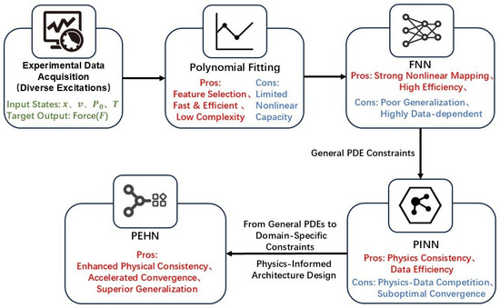
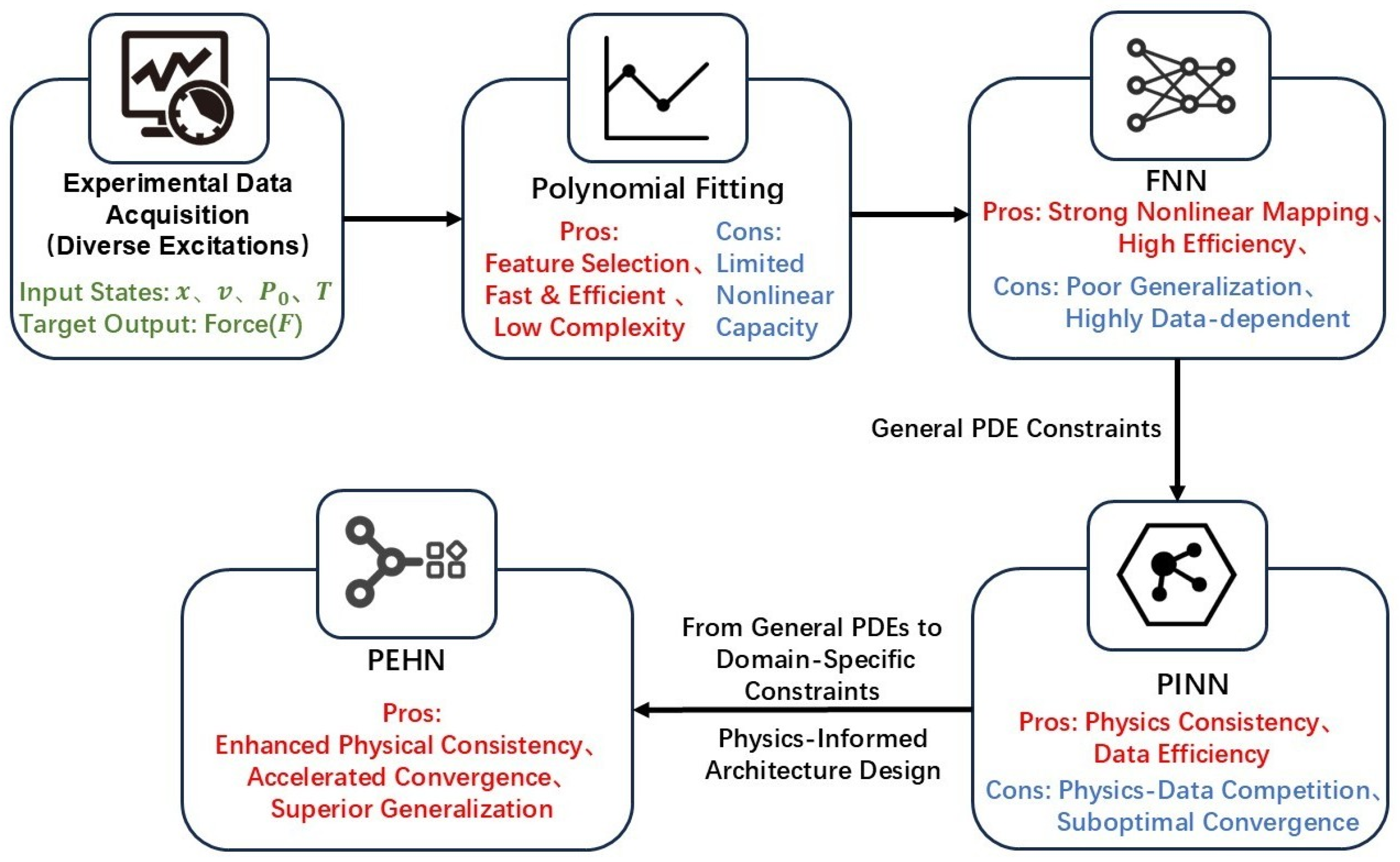
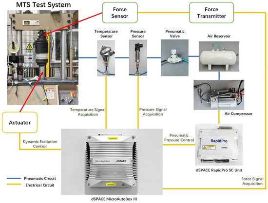
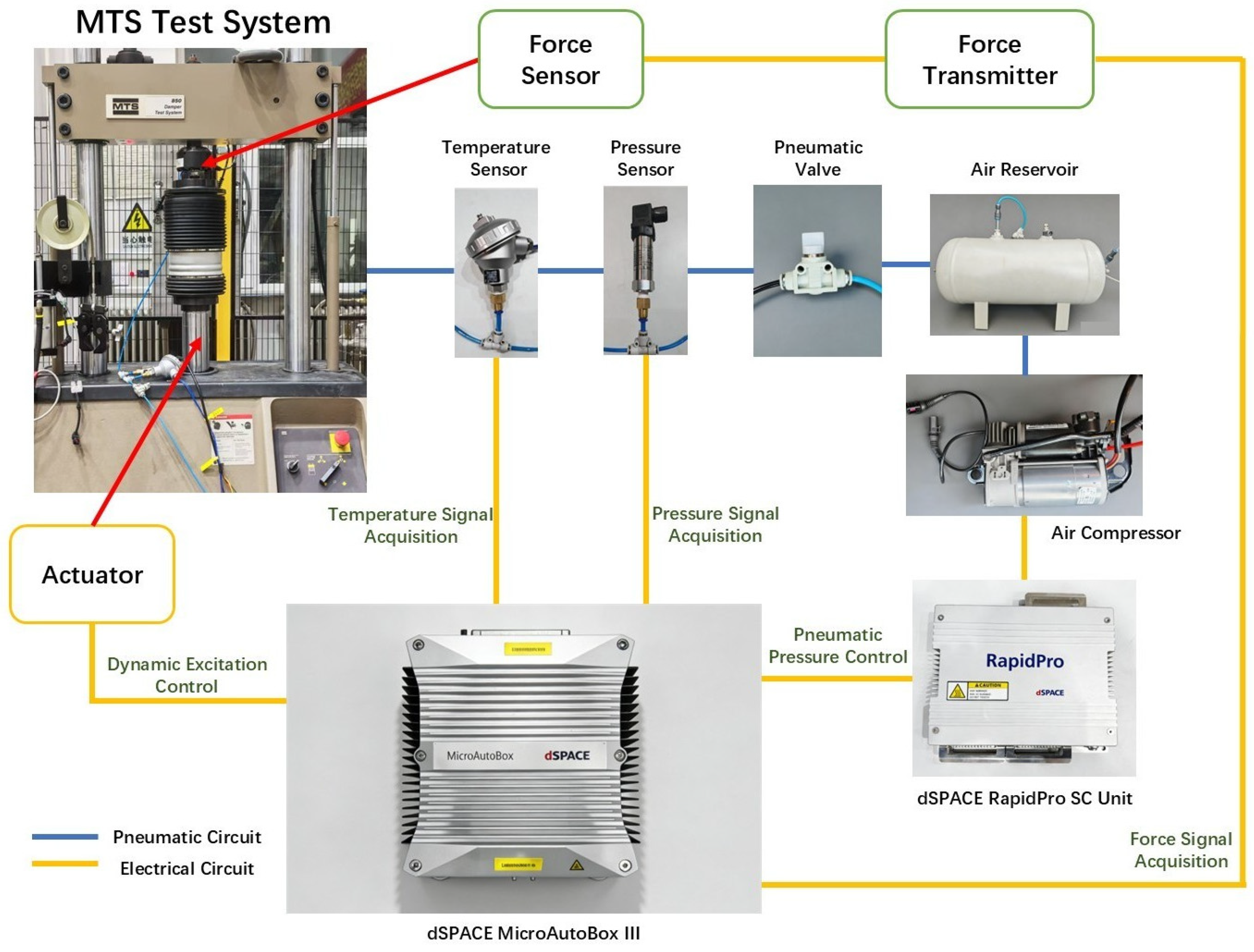
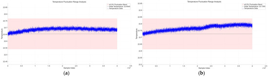
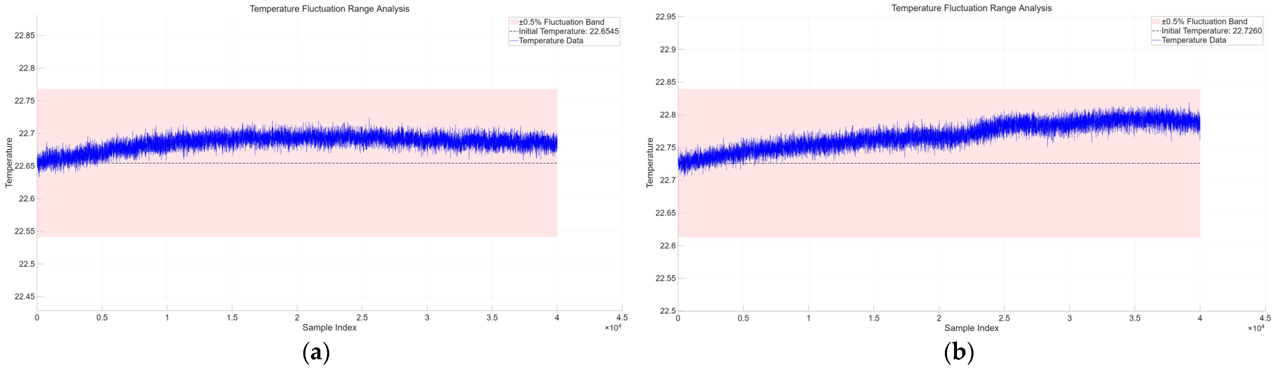
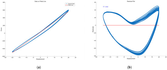
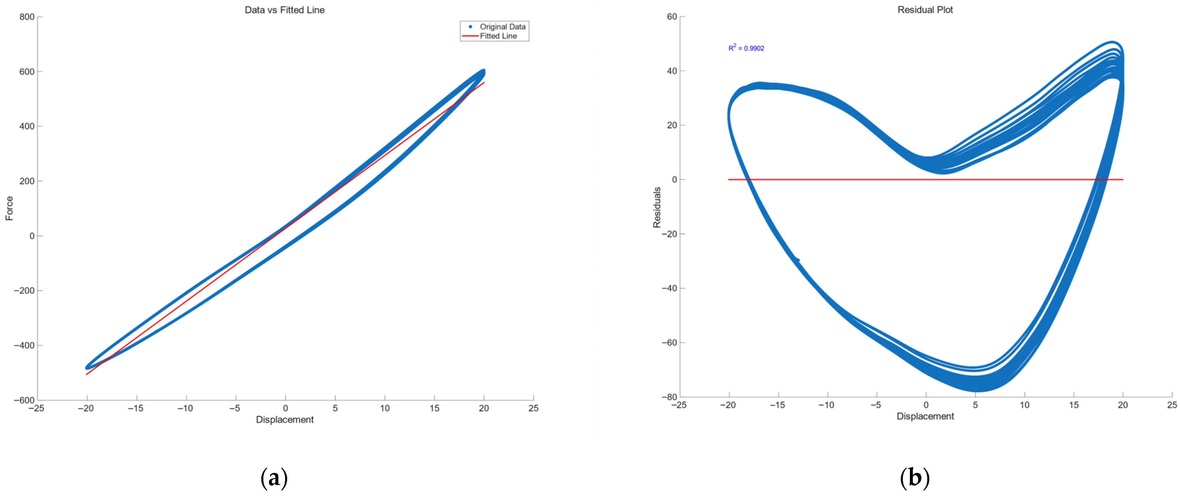
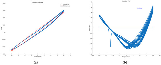
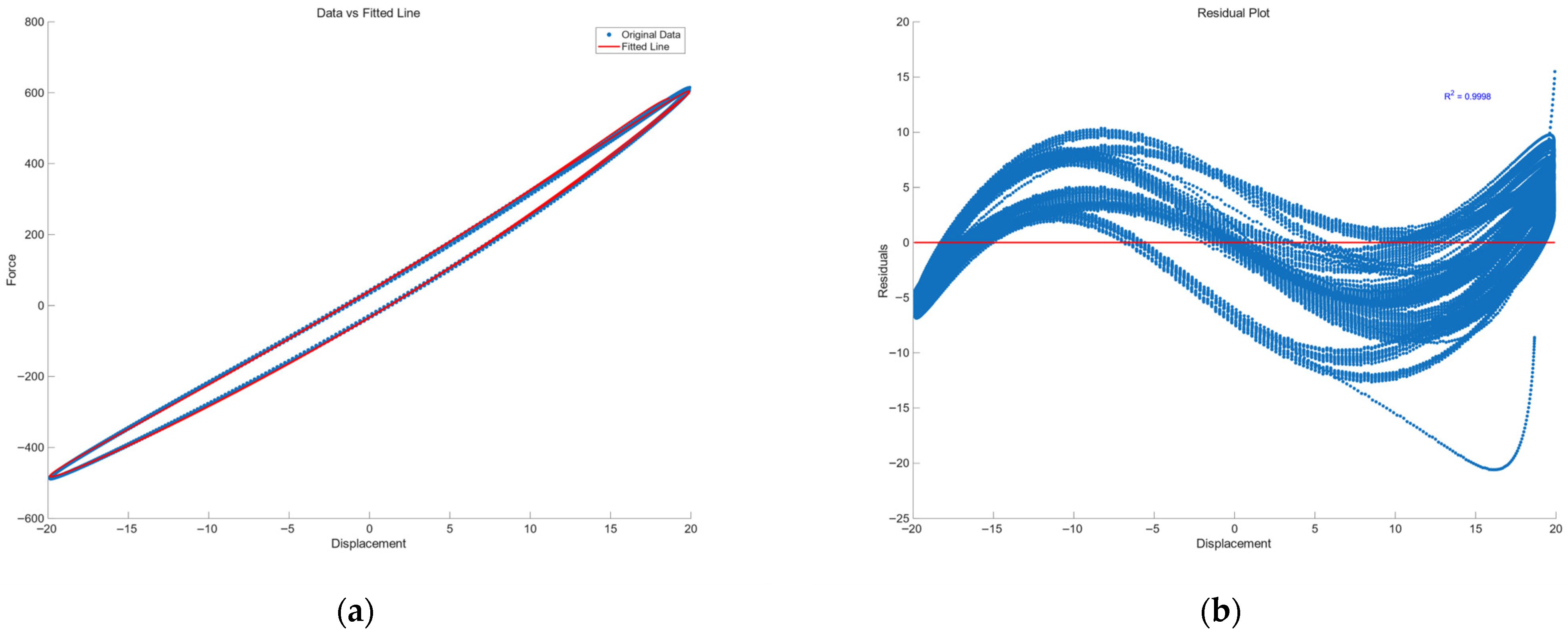
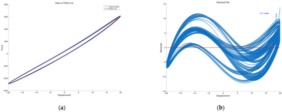
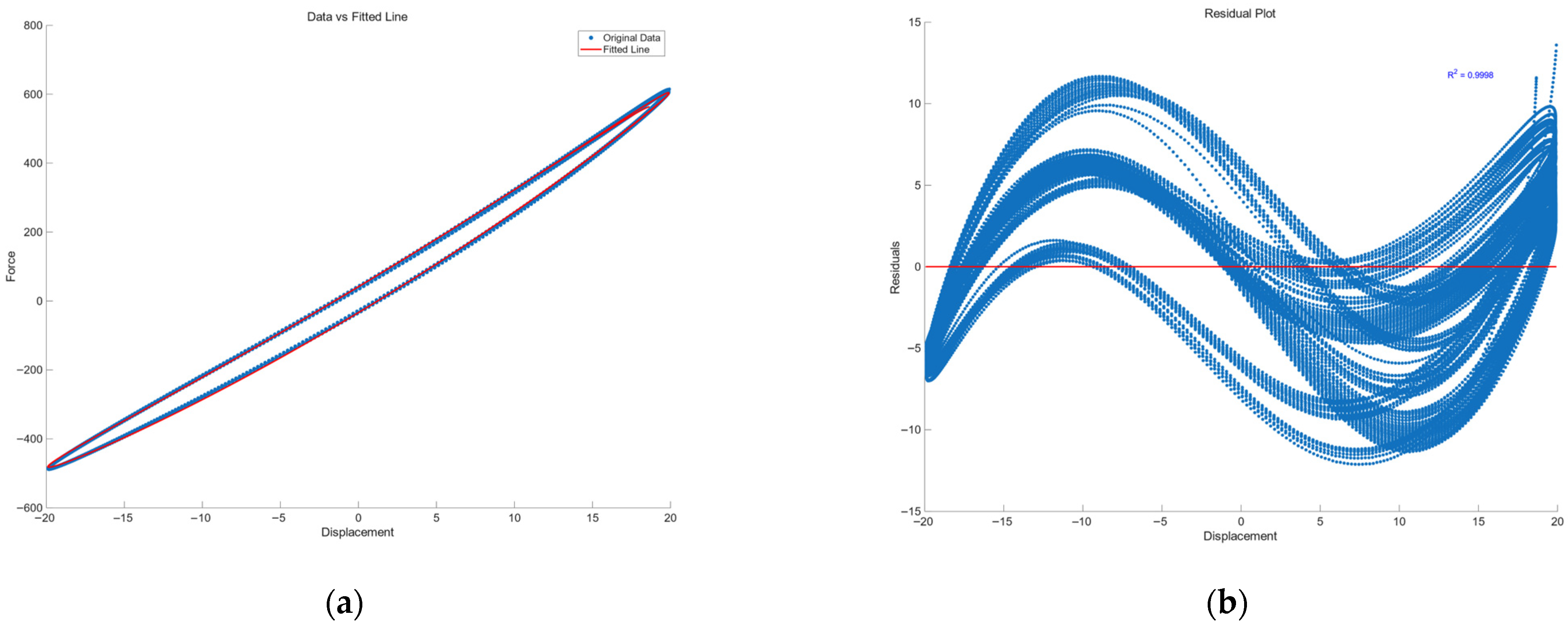
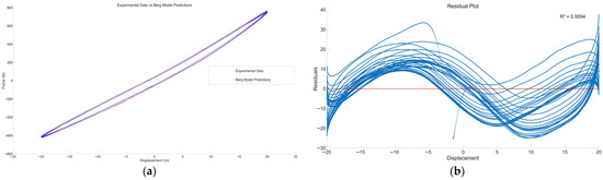
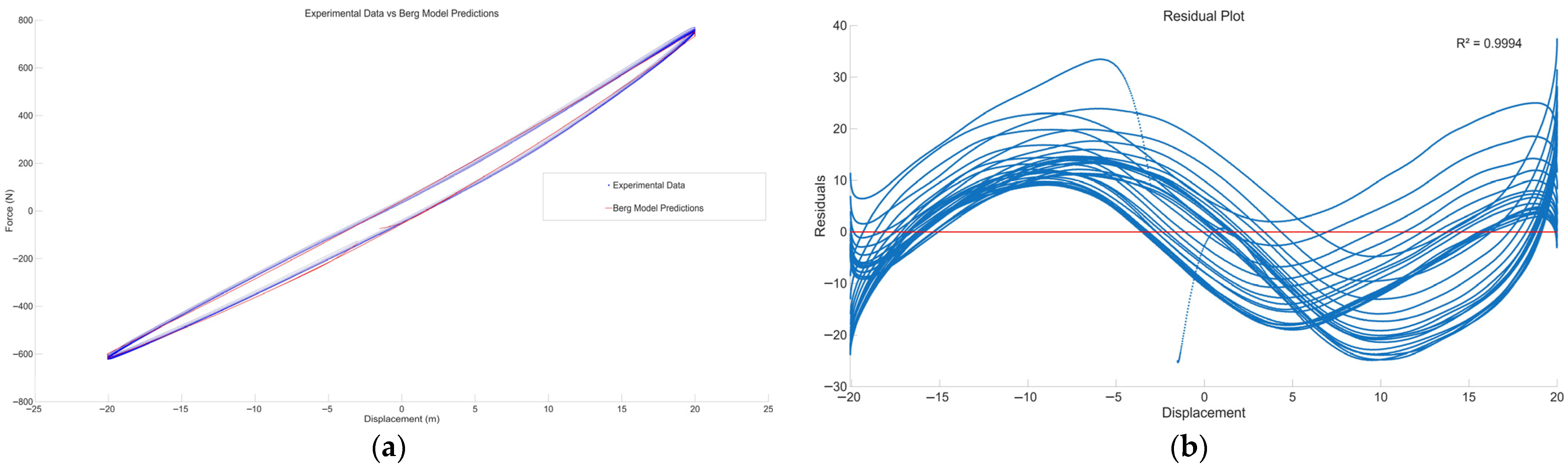
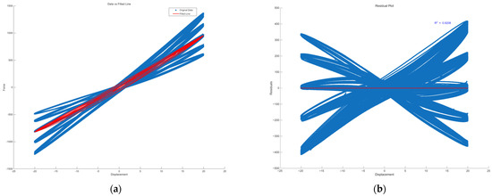
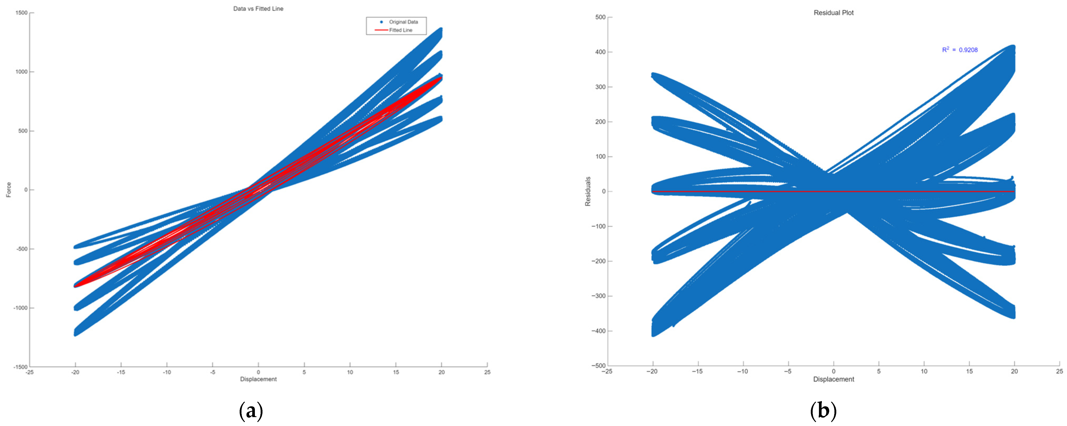
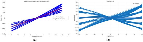
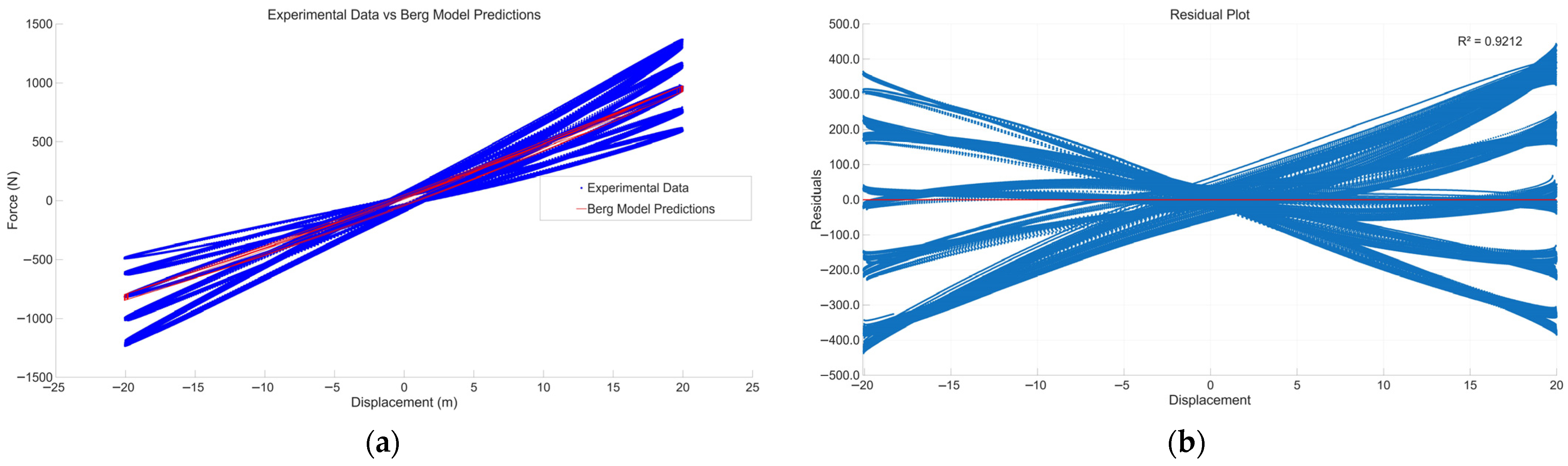
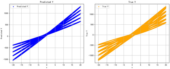
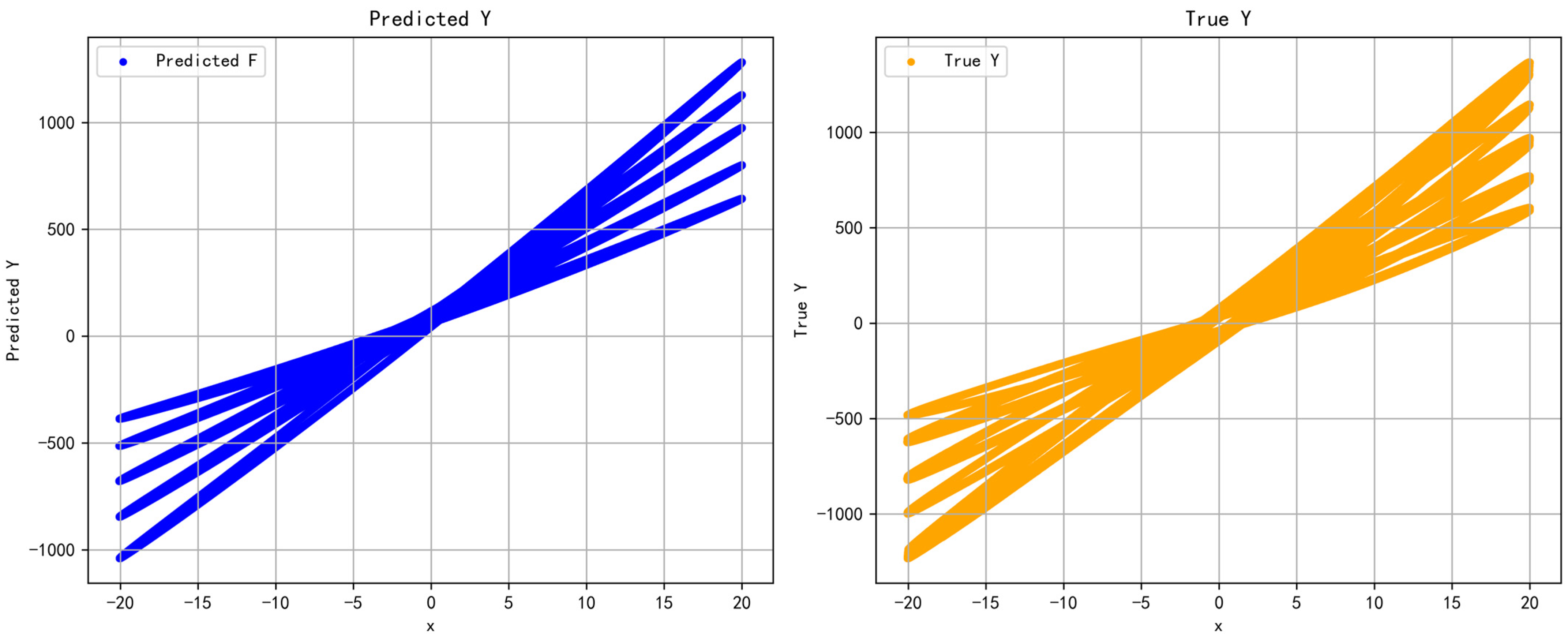
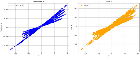
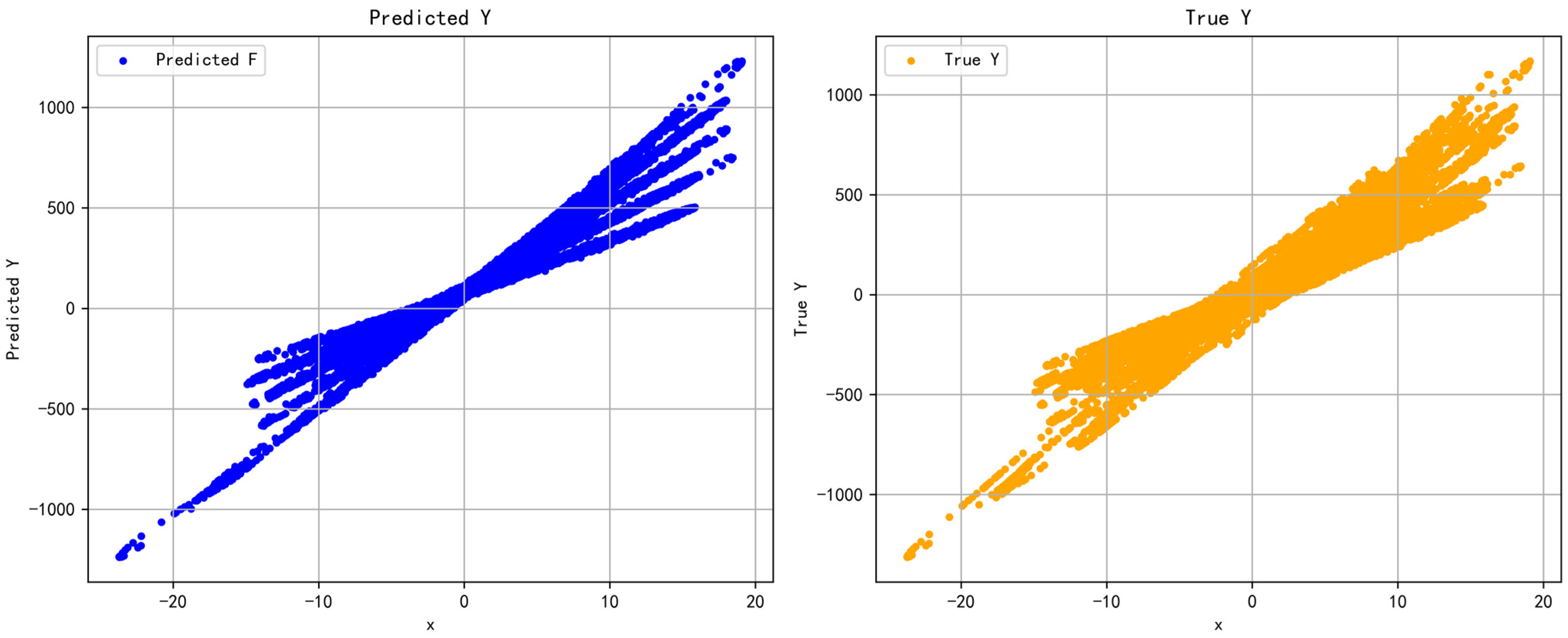
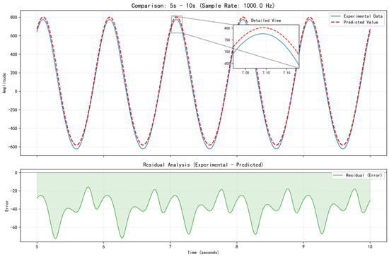
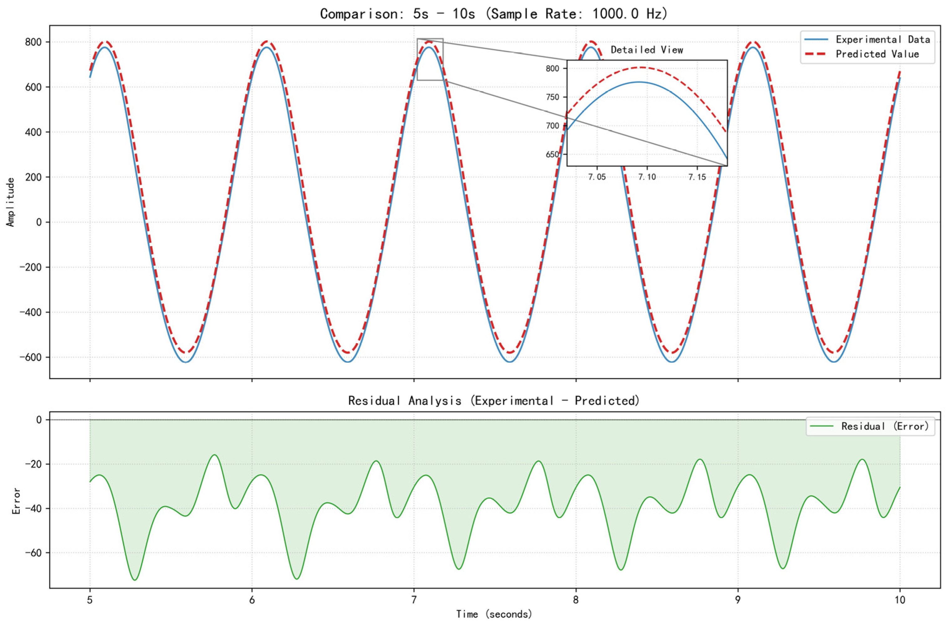
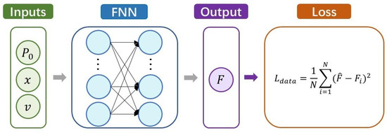
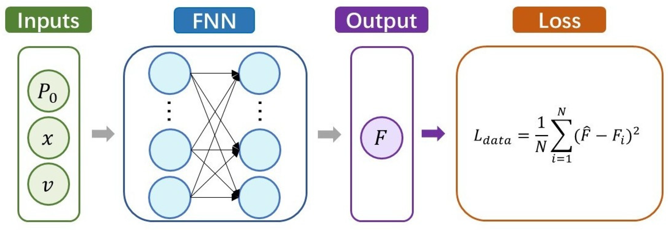
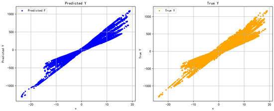
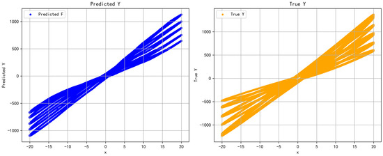
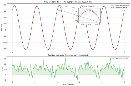
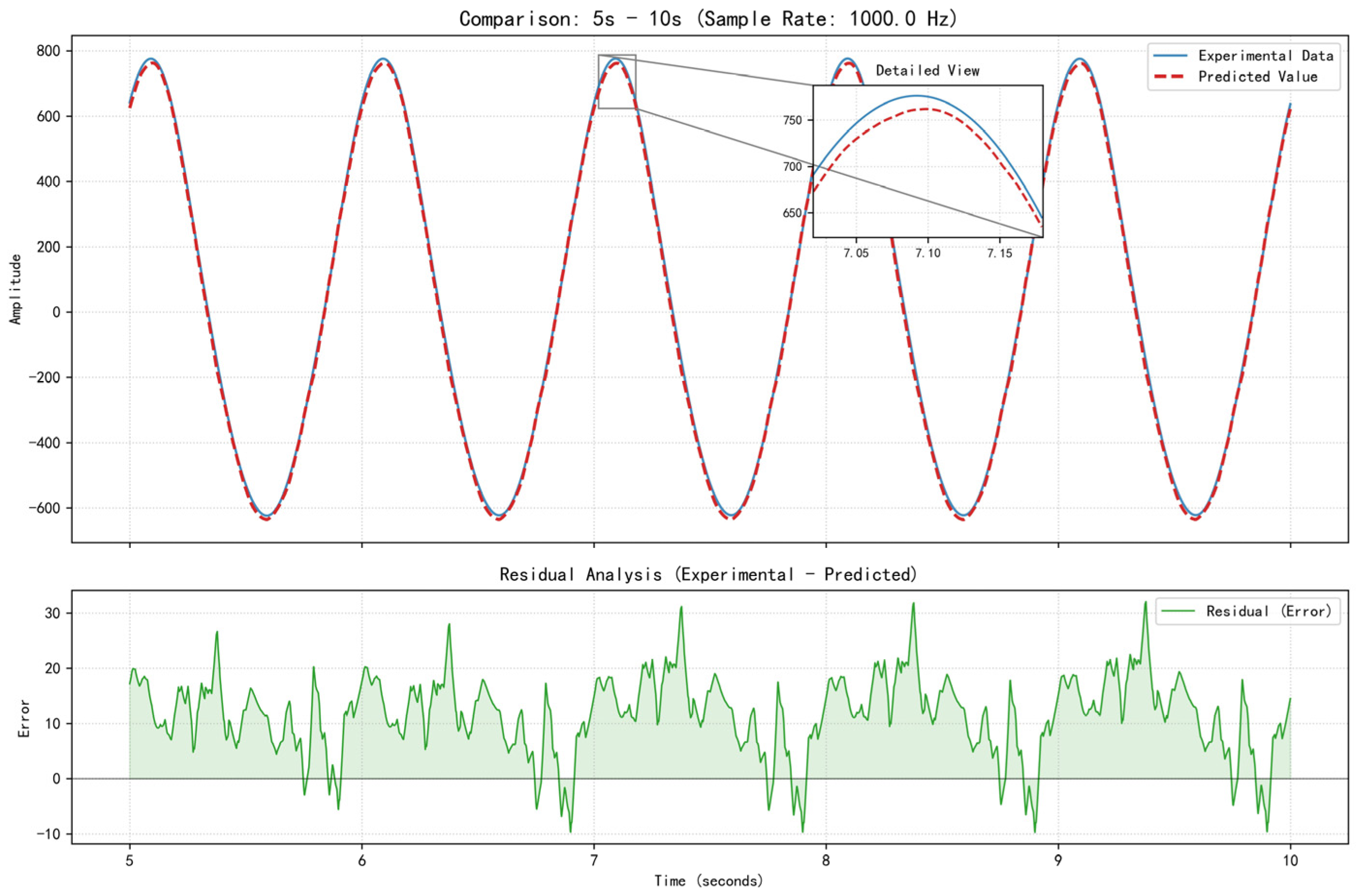
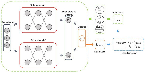
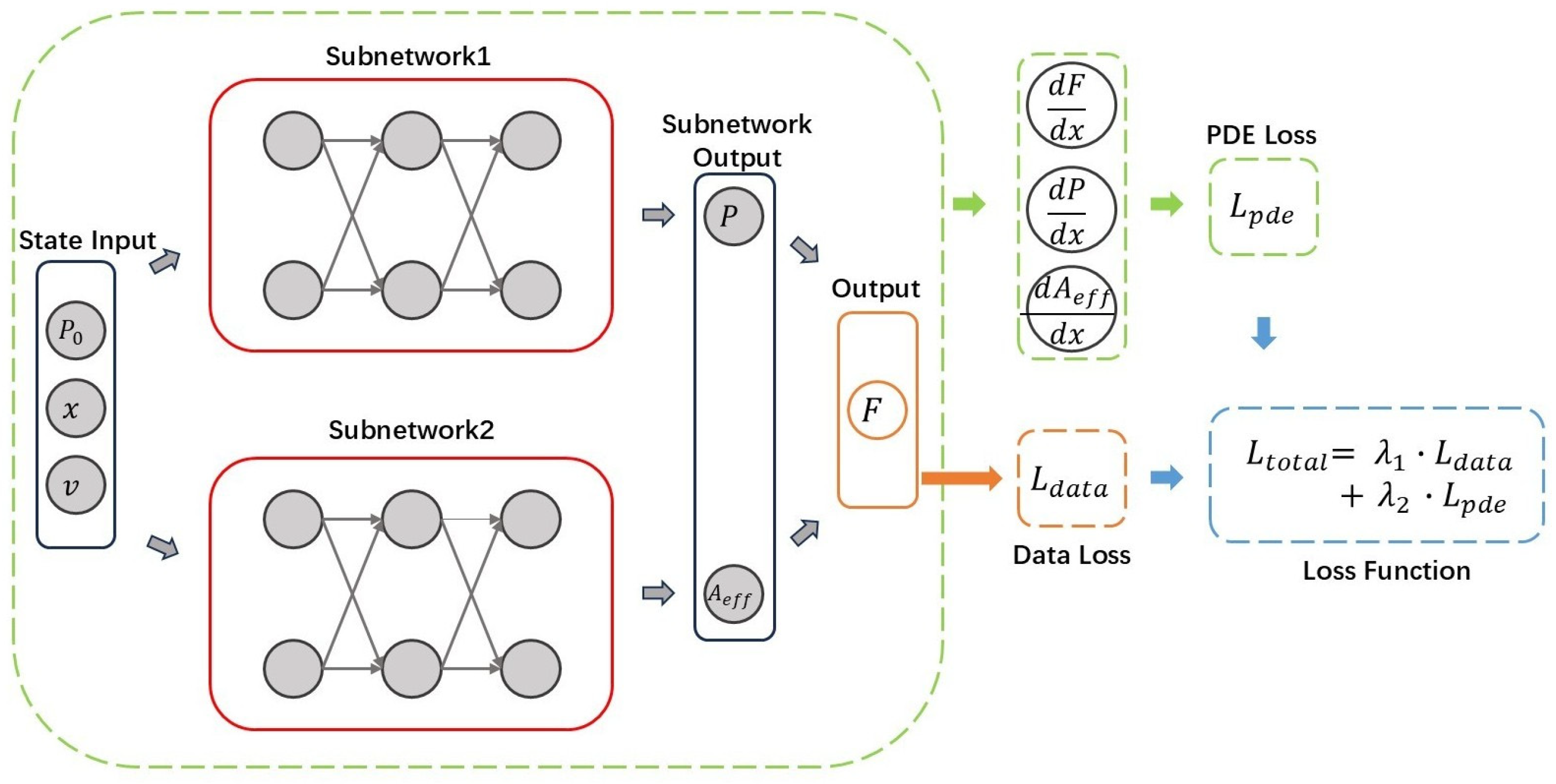
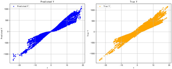
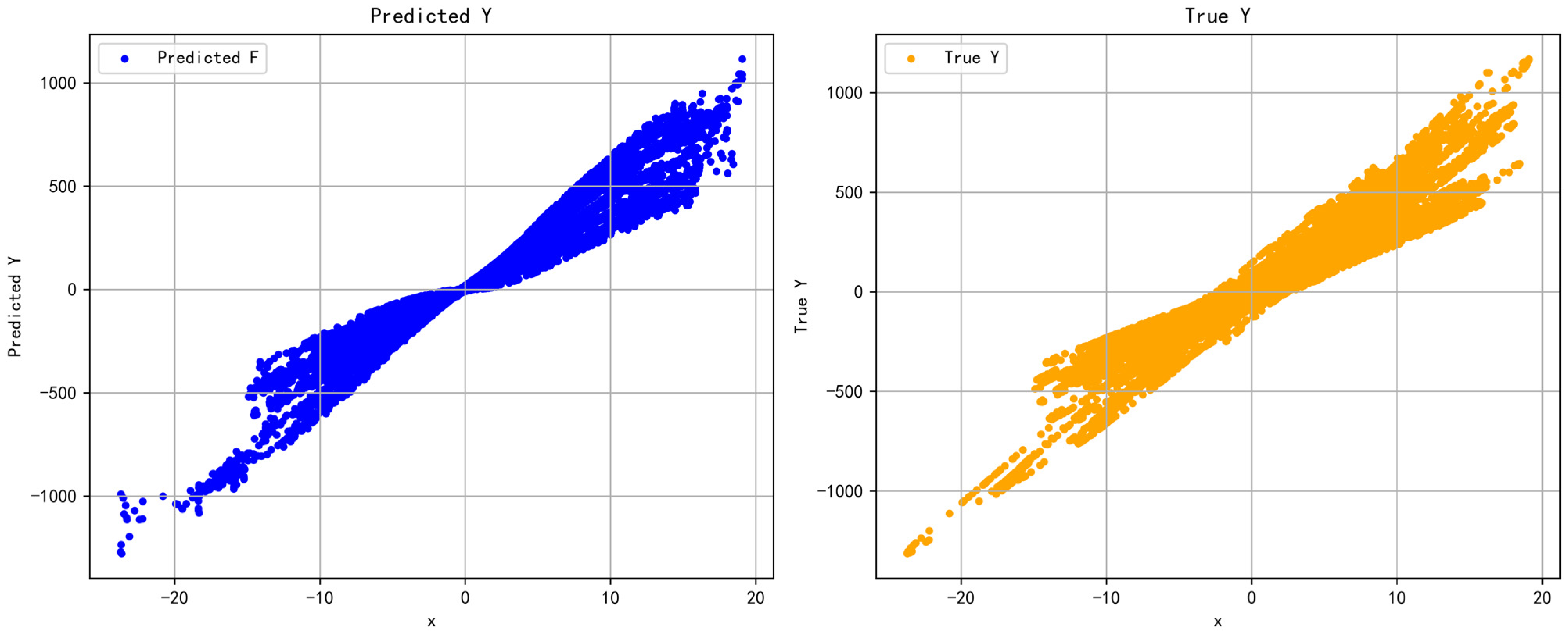
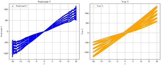
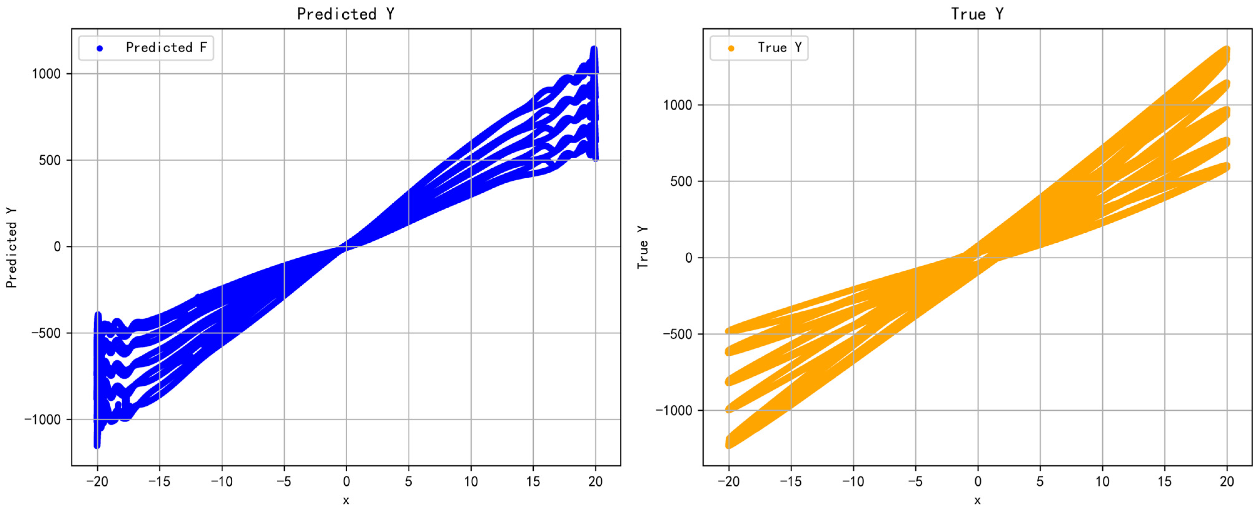
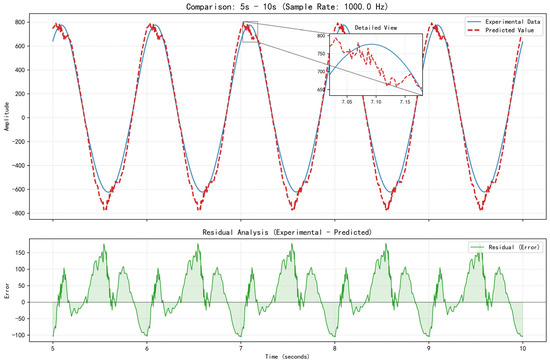
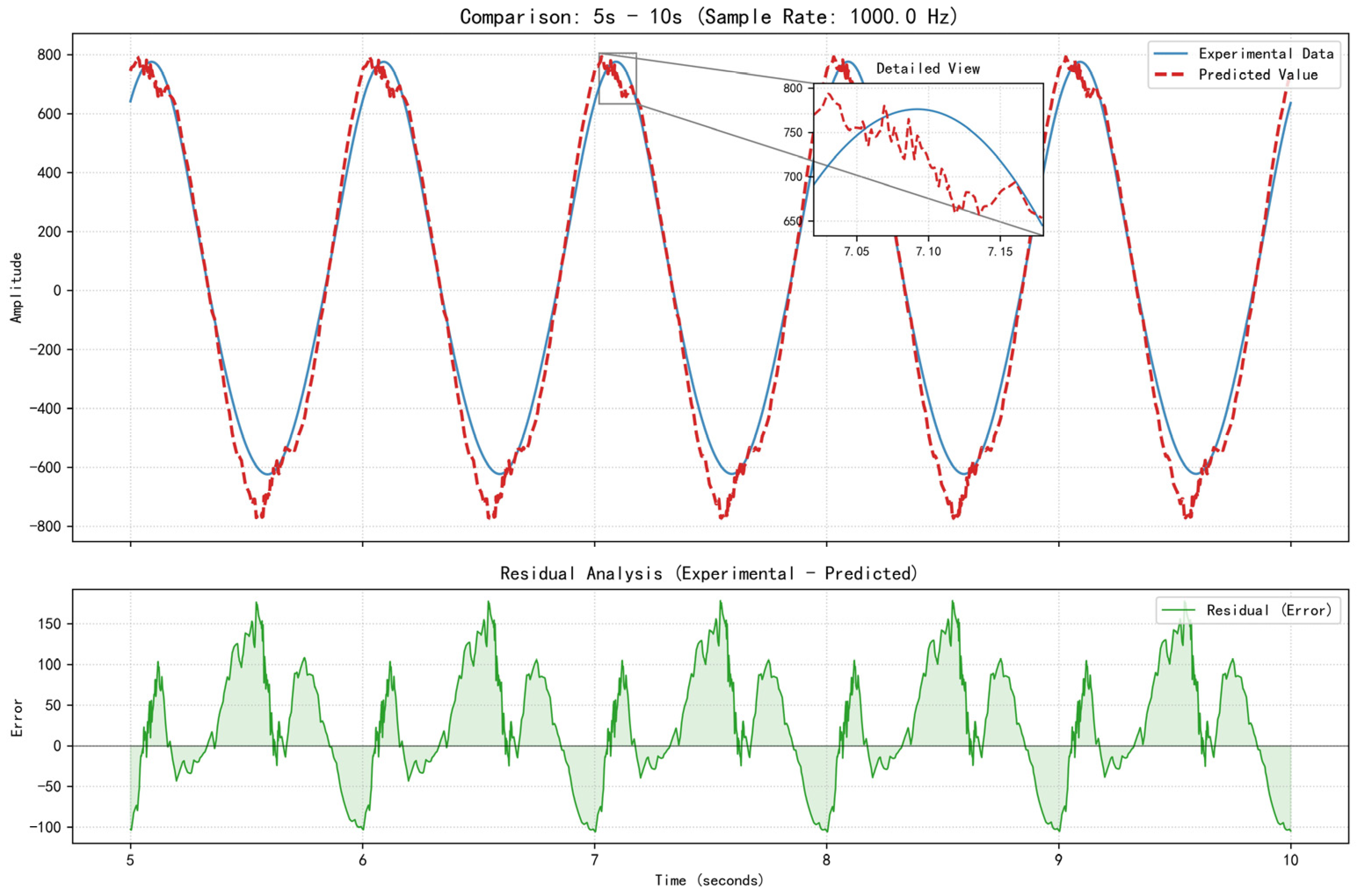
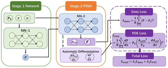
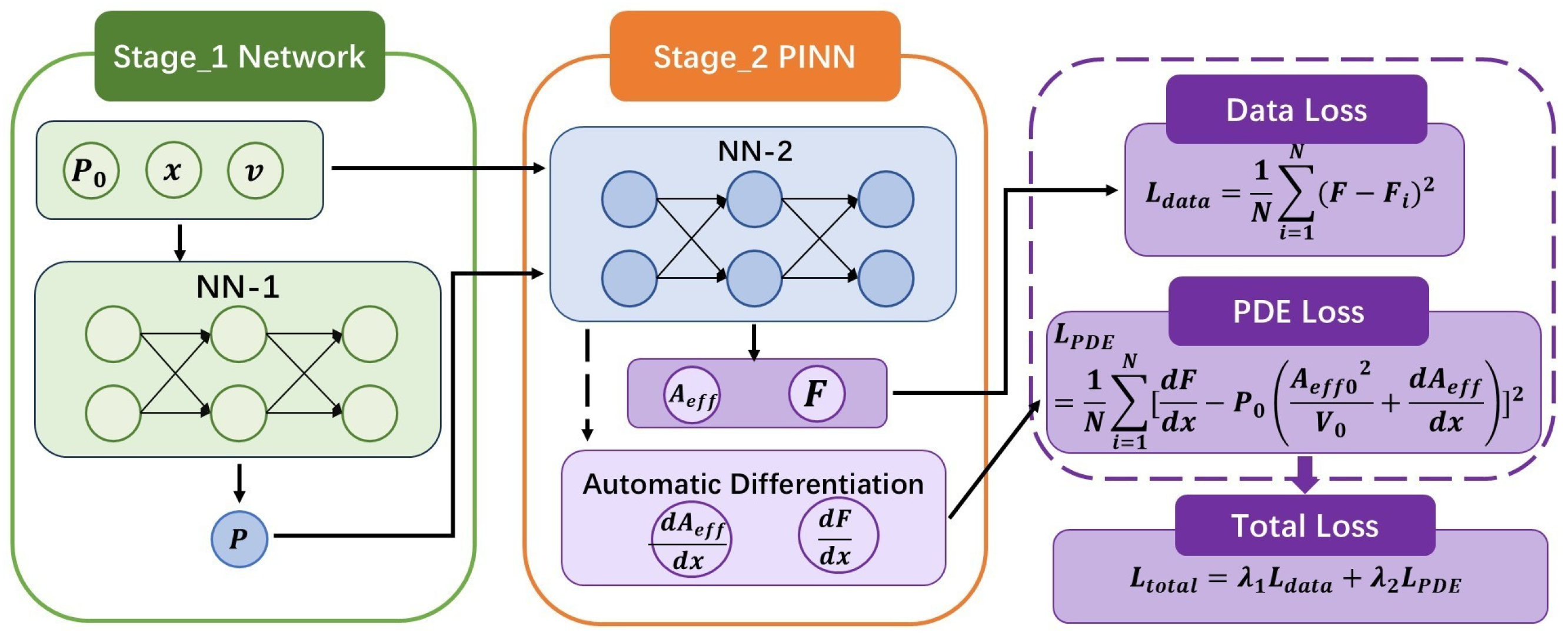
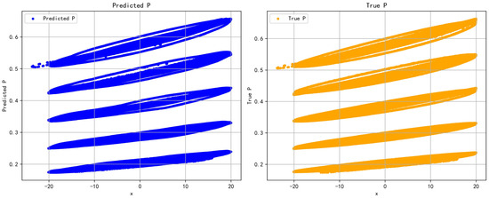
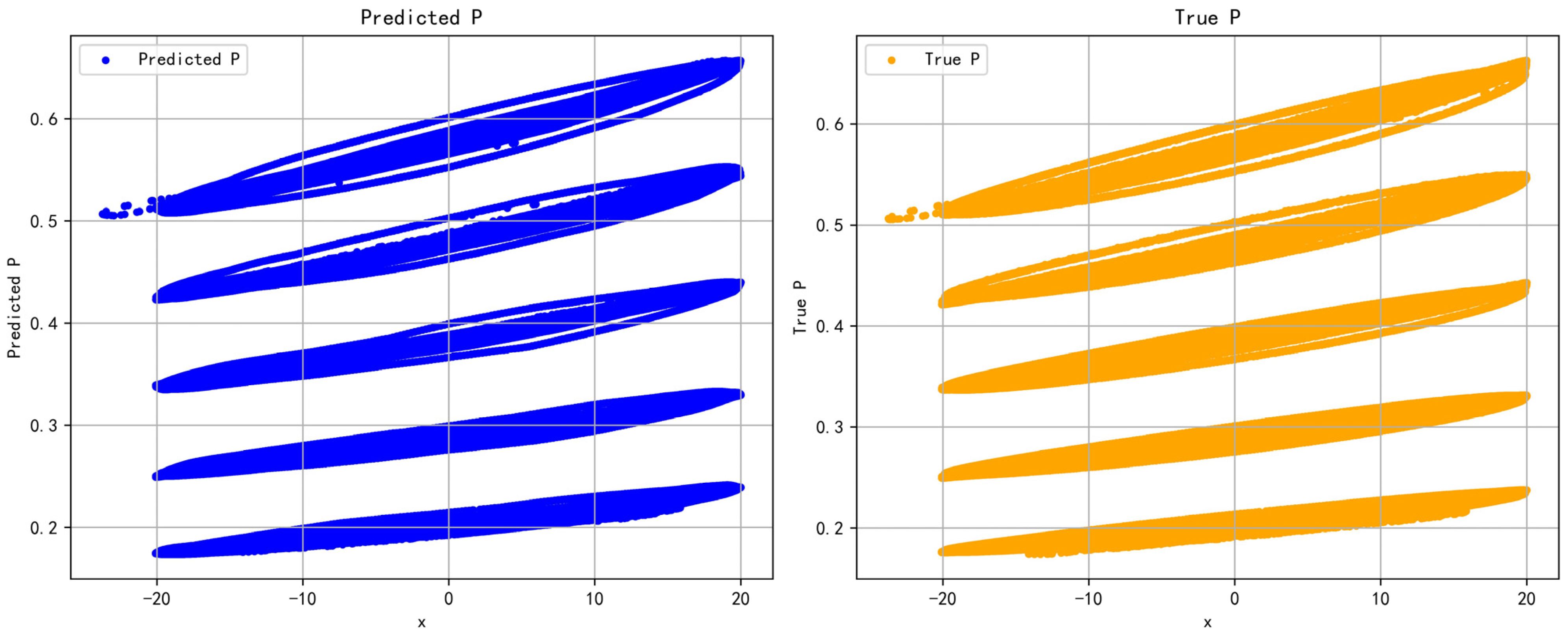
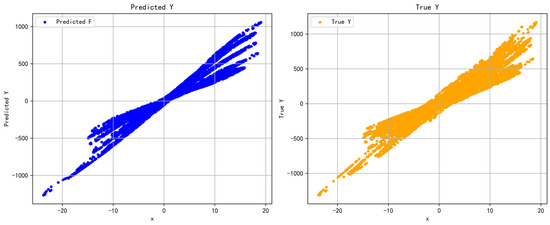
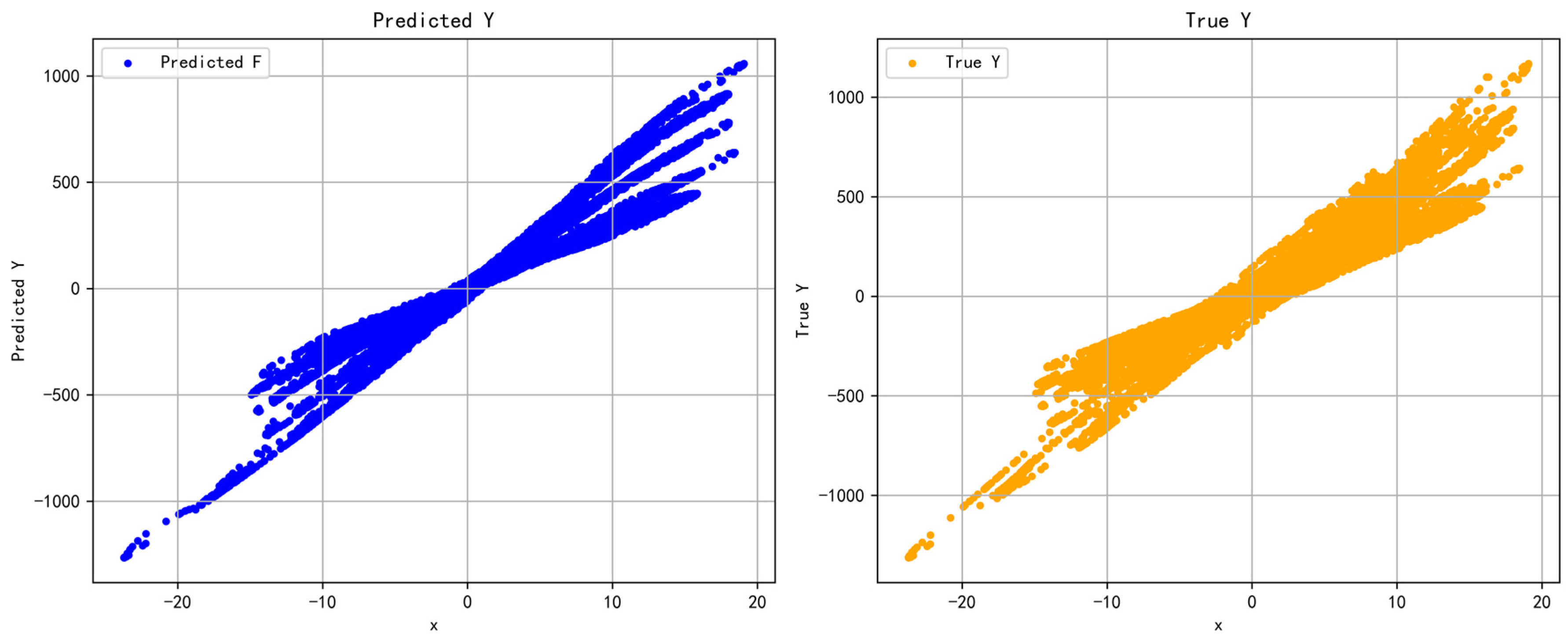
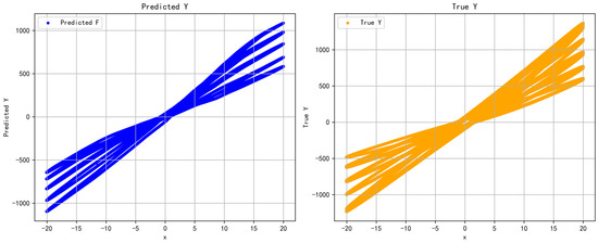
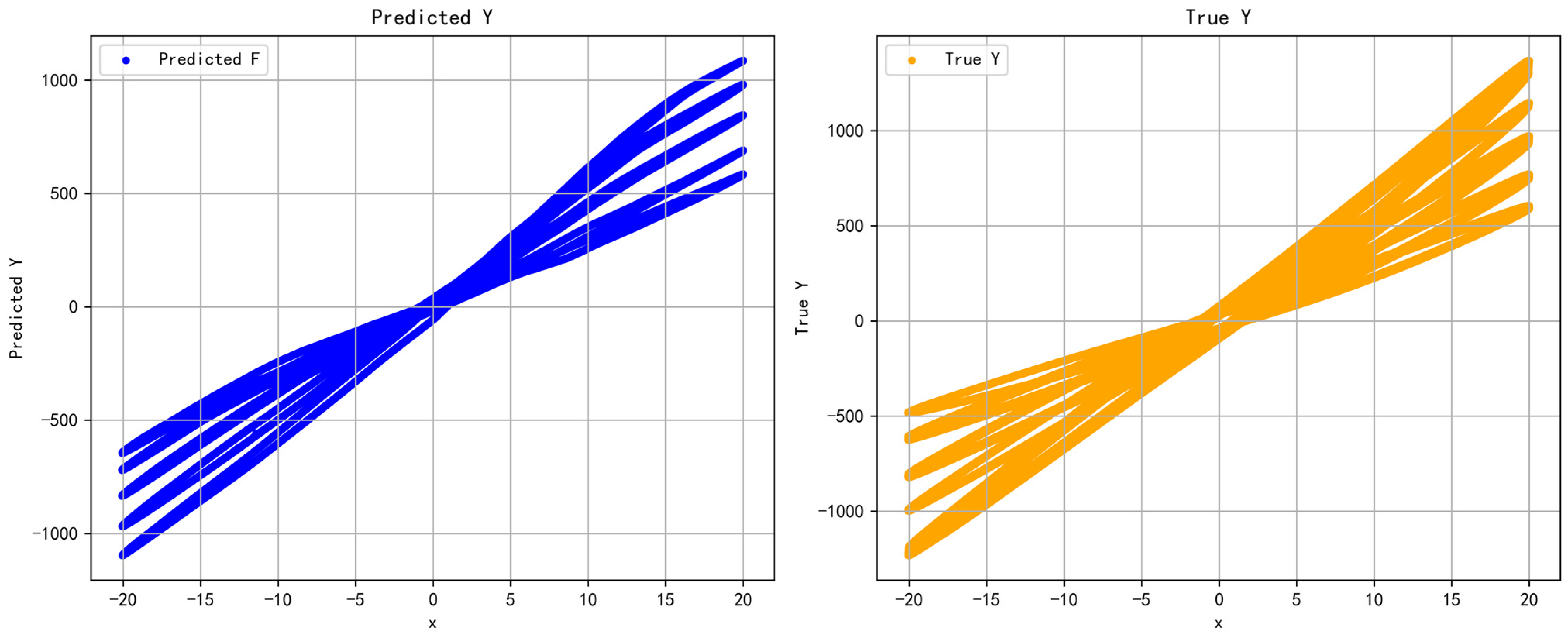
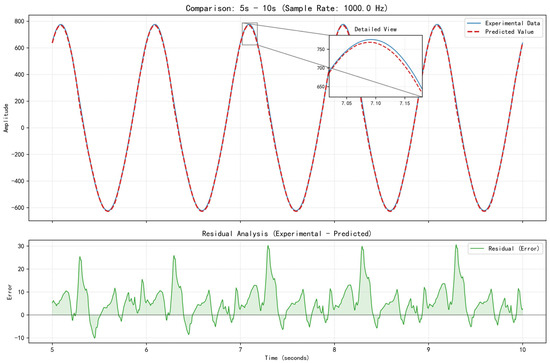
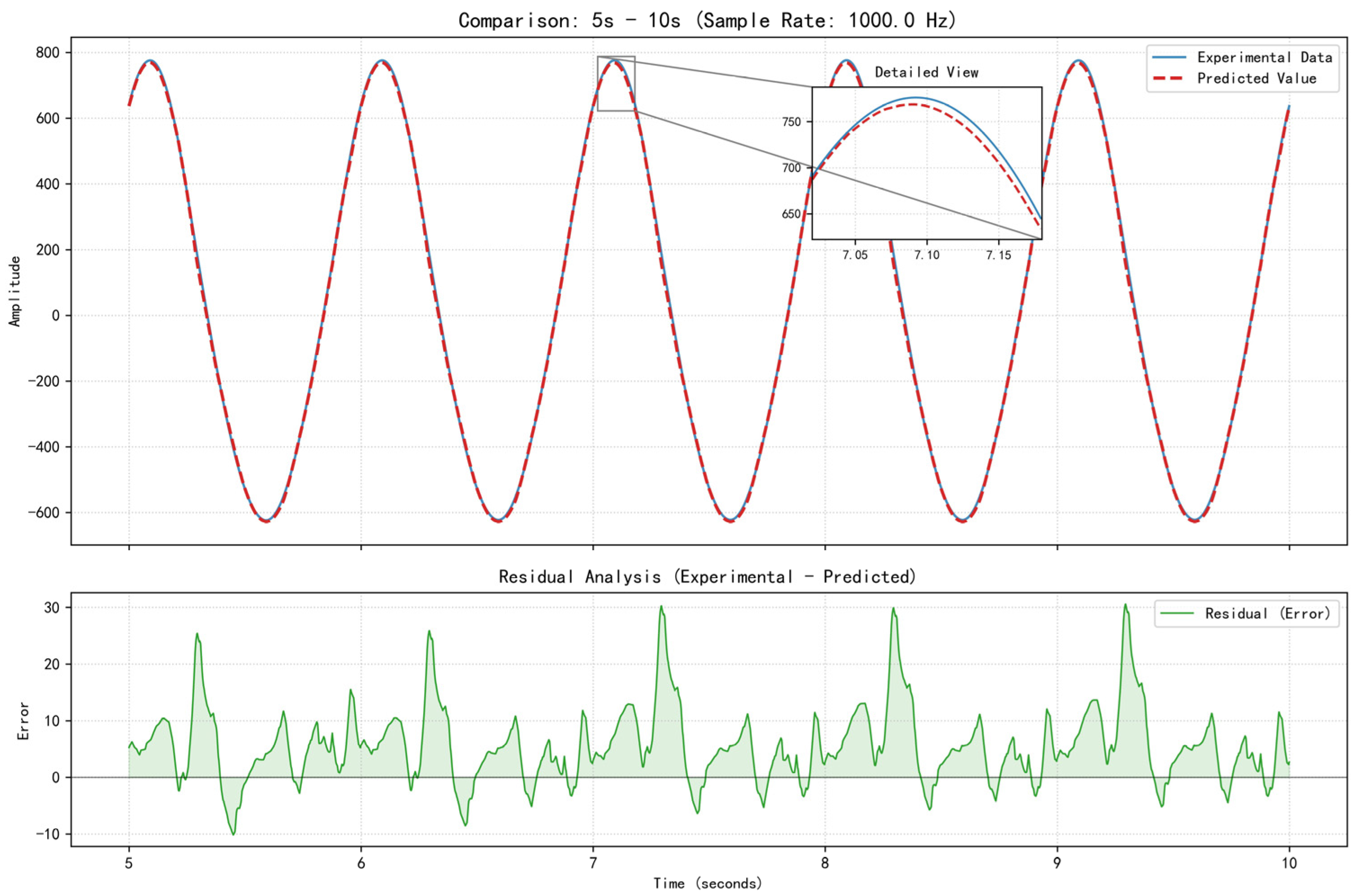

Disclaimer/Publisher’s Note: The statements, opinions and data contained in all publications are solely those of the individual author(s) and contributor(s) and not of MDPI and/or the editor(s). MDPI and/or the editor(s) disclaim responsibility for any injury to people or property resulting from any ideas, methods, instructions or products referred to in the content. |
© 2026 by the authors. Licensee MDPI, Basel, Switzerland. This article is an open access article distributed under the terms and conditions of the Creative Commons Attribution (CC BY) license.