


Abstract
Parallel iterative schemes are widely used for the simultaneous computation of all distinct roots of nonlinear equations in scientific computing and engineering. While high-order parallel methods can provide substantial acceleration, their practical performance is often dominated by the choice of internal real-valued parameters introduced by correction/acceleration mechanisms, which may strongly affect convergence speed and numerical robustness. Classical parameter-selection strategies—based on analytical sufficient conditions, trial-and-error experimentation, or qualitative dynamical diagnostics (basins of attraction, bifurcation-style inspection, and parameter planes)—are typically problem-dependent, expensive to scale, and difficult to automate reproducibly. In this work, we propose a data-driven framework for systematic parameter optimization based on finite-time contractivity profiling. The approach uses k-nearest neighbors (kNN) micro-series analysis to estimate a proxy profile of the largest Lyapunov exponent (LLE) along the iteration index, summarizing the transient contraction/expansion behavior of the solver trajectories. Two profile-based scores, the minimum score and the moment score , are introduced to rank candidate parameter pairs and to construct stability landscapes over grids. As a testbed, we apply the framework to a bi-parametric two-step parallel Weierstrass-type scheme and demonstrate that the learned parameter regions yield faster and more reliable convergence than generic or manually tuned choices. Extensive numerical experiments show that the proposed profiling-based optimization consistently improves convergence rate and robustness across the considered nonlinear test problems, providing a scalable and reproducible alternative to heuristic and dynamical-system-based tuning.
Keywords:
parallel root-finding; parameter tuning; machine learning; k-nearest neighbors; largest Lyapunov exponent; finite-time contractivity; numerical robustness MSC:
65Yxx; 68T05; 68T45; 65H04; 65H05; 65H17
1. Introduction
Nonlinear equations constitute a central pillar of mathematical modeling in science, engineering, and applied technology. Problems arising in fluid mechanics, chemical reaction networks, electrical circuits, biomedical engineering, control theory, optimization, and signal processing frequently reduce to the computation of the roots of nonlinear scalar or vector-valued functions [1,2], often in settings where robustness and numerical stability are more critical than extreme precision. In particular, polynomial and polynomial-like nonlinear systems play a crucial role in eigenvalue computations [3], spectral methods [4], stability analysis [5], inverse problems [6], and discretizations of differential and integral equations [7,8]. The reliable and efficient numerical solution of nonlinear equations is therefore a long-standing and continuously evolving research area in numerical analysis. Among the available numerical techniques, iterative root-finding methods are especially attractive due to their conceptual simplicity, flexibility, and scalability. Classical single-root methods such as Newton [9], Halley [10], and Chebyshev schemes [11] are well known for their local convergence properties and high asymptotic convergence orders. However, in many applications, especially those involving high-degree polynomials or large-scale systems, it is not sufficient to compute a single root; rather, all distinct roots must be obtained simultaneously with high accuracy and robustness. This requirement has motivated the development of parallel and simultaneous iterative schemes, among which the Weierstrass (or Durand–Kerner) method [12] and its variants occupy a prominent position. Parallel root-finding methods are particularly well-suited for modern computational architectures, including multicore processors, GPUs, and distributed systems. Their ability to compute all roots simultaneously not only reduces computational cost but also avoids deflation procedures, which may introduce numerical instability and error propagation [13]. Consequently, the design, analysis, and acceleration of parallel iterative schemes remain an active and significant area of research.
Despite their widespread use, classical single-root iterative methods suffer from several well-known limitations:
- First, their convergence is typically local, requiring initial guesses sufficiently close to the desired root.
- Second, they are highly sensitive to the choice of initial values, particularly in the presence of multiple or closely spaced roots.
- Third, when applied sequentially to compute multiple roots, they often rely on deflation techniques, which may degrade numerical stability and amplify rounding errors.
Parallel methods, such as the classical Weierstrass scheme, overcome some of these difficulties by computing all roots simultaneously and avoiding deflation. However, they introduce their own challenges. The original Weierstrass method exhibits quadratic convergence under suitable assumptions, but its performance may deteriorate for ill-conditioned problems, clustered roots, or poorly chosen initial approximations. Moreover, the convergence behavior of parallel schemes is often strongly influenced by nonlinear interactions among the approximations of different roots, leading to complex dynamical phenomena [14,15]. To enhance the efficiency of parallel schemes, various correction strategies have been proposed, including single-step and multi-step modifications designed to increase the convergence order from two to three or higher [16]. While these higher-order schemes offer faster asymptotic convergence, they frequently involve additional parameters whose values critically affect stability, convergence rate, and robustness. Selecting appropriate parameter values is therefore a nontrivial and problem-dependent task.
A substantial body of literature has been devoted to the construction of high-order parallel root-finding methods and to the study of their convergence properties. Classical approaches to parameter selection and method assessment rely on analytical convergence analysis, numerical experiments, and tools from real and complex dynamical systems [17,18]. These include parametric planes [19], bifurcation diagrams [20], critical point analysis [15], and fractal visualizations [21]. While such techniques provide deep qualitative insight into the dynamical behavior of iterative schemes, they also exhibit notable limitations. First, they are often computationally expensive, especially when exploring multi-dimensional parameter spaces. Second, their interpretation may be subjective and heavily dependent on visualization choices. Third, they do not easily scale to large families of methods or to automated parameter optimization. As a result, there remains a clear gap between the theoretical development of parameterized parallel schemes and the systematic, data-driven selection of optimal parameters. Recent advances in machine learning and data-driven modeling [22,23] offer new opportunities to address this gap. In particular, our recent work (Velichko et al. [22]) introduced and validated a machine-learning-based methodology for the largest Lyapunov exponent estimation from multi-horizon forecast-error growth in one-dimensional chaotic time series, demonstrating strong practical accuracy and robustness. In the present paper, we do not reintroduce that methodology as a new standalone estimator; instead, we adapt its core forecasting-error-growth principle to finite-time contractivity profiling and parameter ranking for a parallel root-finding scheme. However, the integration of machine learning techniques into the design and tuning of parallel root-finding methods remains relatively unexplored.
Parallel root-finding schemes are of increasing importance in both theory and practice. From a theoretical standpoint, they provide a natural framework for studying collective dynamics, stability, and interaction effects among approximations to different roots. From a practical standpoint, they are well aligned with modern high-performance computing environments and enable efficient large-scale computations [24].
The efficiency of parameterized parallel schemes, however, strongly depends on the chosen internal parameters. Traditional tuning relies on analytical sufficient conditions, trial-and-error testing, and qualitative dynamical diagnostics such as parameter planes and basins of attraction. While useful, these approaches are often manual, time-consuming, problem-dependent, and difficult to scale reproducibly, especially when the scheme exhibits sensitive transient dynamics.
1.1. Digital Health Motivation
Beyond classical scientific computing, nonlinear root-finding arises naturally in digital health and occupational safety, where a personal digital assistant must continuously integrate heterogeneous sensor streams (wearables, bedside devices, mobile telemetry, and contextual/environmental sensing) into actionable health services [25]. In many physiological and biochemical pipelines, reduced-order dynamical models are calibrated online, and their operating regimes are characterized by equilibria or steady states; these states are frequently computed by repeatedly solving nonlinear algebraic balance equations (or polynomial surrogates) under changing conditions [26]. Since feasibility and safety are closely tied to stability of the underlying model, stability- and resilience-reflecting constraints are often used to restrict admissible parameter sets and to screen out unstable regimes [27]. Practically, this implies repeated re-initialization and frequent re-calibration at scale, motivating robust and computationally efficient solvers and tuning procedures, including parallel and self-adaptive strategies that reduce wall-clock time while maintaining reliability [28]. Similar repeated estimation loops also appear in contactless vital-sign monitoring, where adaptive nonlinear estimation must remain stable under noise, motion, and nonstationarity [29]. In this context, the proposed finite-time contractivity profiling via a kNN micro-series largest Lyapunov exponent (LLE) proxy provides a lightweight stability indicator for selecting solver parameters that remain reliable across operating conditions and are suitable for reproducible deployment on multicore/edge platforms, complementing earlier step-log contraction profiling results [30].
In this work, we adopt a data-driven alternative based on finite-time contractivity profiling. Specifically, we construct a k-nearest neighbors (kNN) micro-series estimator of the largest Lyapunov exponent (LLE) proxy profile along the iteration index, which serves as a quantitative indicator of local contraction or expansion in the solver dynamics. The rationale for using kNN is that stability is inherently local: by comparing only nearby micro-series windows (in the space of short trajectory segments), the estimator captures local error-growth behavior without imposing a global parametric model. The resulting profile serves as an interpretable finite-time indicator: negative values correspond to locally contractive behavior, whereas positive values indicate transient instability. To enable systematic parameter selection, the profile is summarized by two scalar scores computed from the smoothed profile: the stability minimum and the stability moment . These metrics quantify the depth and temporal concentration of contractive behavior and allow consistent ranking of candidate parameter pairs across test problems. Unlike purely visual diagnostics, the proposed profiling framework yields reproducible stability landscapes over grids and supports automated screening of parameter regions associated with rapid and robust convergence.
1.2. Positioning of the Proposed Framework
Unlike classical basin-of-attraction or bifurcation analyses, which provide primarily qualitative insight, the proposed framework delivers an automated and quantitatively ranked parameter-selection mechanism based on finite-time contractivity profiling. In contrast to generic machine-learning hyperparameter tuning strategies, the approach is explicitly tailored to the dynamical structure of parallel root-finding iterations and exploits short-horizon error-growth behavior as an interpretable stability proxy. This design enables scalable and reproducible screening of parameter regions while preserving a clear connection to the underlying numerical dynamics.
The main contributions of this paper can be summarized as follows:
- -
- A bi-parametric two-step parallel Weierstrass-type scheme, augmented by a single-step correction strategy, increasing the convergence order from two to three while preserving the parallel structure.
- -
- A data-driven, systematic parameter optimization framework based on kNN micro-series LLE-proxy profiling, including smoothing and profile-based ranking via the metrics and .
- -
- Heatmap-based stability landscapes over that reveal structured regions of finite-time contractivity and provide an automated alternative to manual parameter tuning.
- -
- Extensive numerical experiments showing that parameters selected by the proposed profiling framework yield consistent improvements in convergence speed and robustness when computing all distinct roots.
In this context, the primary novelty of the present study lies in the proposed data-driven parameter optimization framework based on kNN–LLE stability profiling; the new bi-parametric parallel scheme is used as a representative demonstration testbed for this methodology. To the best of our knowledge, this is among the first works to employ kNN-based finite-time Lyapunov-proxy profiling to systematically optimize parameters in parallel simultaneous root-finding schemes.
The remainder of this paper is organized as follows: Section 2 introduces the proposed parallel scheme and presents its theoretical convergence analysis. Section 3 describes the profiling framework, including the kNN micro-series methodology and the definition of the performance metrics. Section 4 summarizes the algorithmic workflow of the proposed methodology. Section 5 reports numerical experiments and comparative studies illustrating the effectiveness of the proposed approach. Section 6 concludes the paper and outlines directions for future research.
2. Development, Methodology, and Implementation of the Two-Step Parallel Root-Finding Pipeline
Nonlinear equations arise ubiquitously in science and engineering, with applications spanning fluid dynamics, signal processing, control systems, chemical kinetics, optimization, and biomedical modeling. Accurate and efficient solution of such equations is therefore a fundamental computational task. Classical single-root methods, such as Newton, Halley, and their variants, are widely used due to their simplicity and fast local convergence. However, in many practical problems—especially those involving high-degree polynomials or coupled nonlinear systems—it is desirable to compute all roots simultaneously rather than sequentially.
After the impossibility theorems [31], parallel (simultaneous) methods were developed to approximate all roots of nonlinear equations, particularly polynomials. Consider the general nonlinear equation
If f is a polynomial with n distinct (simple) roots , then it can be written in the factored form
with degree
Owing to their global convergence, enhanced stability, reliability, and natural suitability for parallel architectures, such simultaneous schemes have become central tools in modern polynomial root-finding and large-scale nonlinear computations. Their ability to compute both distinct and multiple roots concurrently makes them especially effective for high-degree polynomials and large-scale nonlinear problems [32]. The simplicity of these methods, their global convergence properties, and their independence from derivative evaluations render them robust and widely adopted in scientific and engineering computations. Moreover, their inherently parallel structure enables efficient implementation on modern multicore processors, GPU architectures, and distributed platforms, thereby facilitating fast, reliable, and scalable root-finding across a broad range of applications.
In this section, we first propose inverse parallel schemes and then present a detailed exposition of our methodology, including the mathematical formulation of the iterative scheme, the motivation for employing Lyapunov analysis, the micro-series kNN-based Lyapunov estimator, the experimental setup, and the organization of the numerical results.
Among the classical schemes, the well-known Weierstrass–Durand–Kerner method [33], which exhibits local quadratic convergence, updates the approximations of the n roots () at iteration according to
Nourein’s method [34] is defined as
where
Zhang et al. [35] introduced the fifth-order method (denoted by ZHM) as
where
and
Several researchers have also proposed multi-step simultaneous root-finding schemes, see, e.g., [36,37,38,39,40,41] and the references therein.
2.1. An Optimal Bi-Parametric Modified Newton Method
Here, we first propose a single-step optimal bi-parametric family for nonlinear equations. This scheme is subsequently embedded as a correction stage within a simultaneous framework and later optimized using kNN–LLE Lyapunov profiling to identify high-performance parameter regimes, ensuring fast and stable convergence for both single-root and simultaneous nonlinear solvers.
The proposed single-root iteration is defined as
Here, the free parameters and act as nonlinear control weights that regulate both the local correction magnitude and the global stability of the iteration. This formulation enables systematic tuning of convergence behavior, which we later exploit through kNN–LLE Lyapunov profiling to extract optimal parameter sets for parallel schemes.
Theorem 1.
Let be an open interval, and let be a simple root of a sufficiently smooth function , i.e., . Define the error by . Then the iterative scheme (7) converges locally to ξ with quadratic order. Moreover, the associated error equation is given by
where
Proof.
Since is a simple root, we have and . Expanding and in Taylor series about yields
Next, expanding the nonlinear weight term gives
Its inverse is
For the composite correction term, we obtain
Finally, the updated iterate satisfies
Remark 1.
The presence of two free parameters enables fine-grained control over both stability and convergence speed. In particular, α primarily scales the local correction magnitude and thus affects the convergence rate, while β influences the coupling and damping of the iterative dynamics, playing a key role in stability; their combined effect is systematically optimized in later sections via kNN–LLE Lyapunov profiling, allowing the method to transition seamlessly from single-root solvers to high-efficiency parallel schemes with superior dynamical stability properties.
2.2. Proposed Parallel Bi-Parametric Scheme for Nonlinear Problems
We start from a parameterized single-root iterative method and incorporate a Weierstrass-type correction to construct a parallel framework for the simultaneous approximation of all simple roots of the nonlinear Equation (1). The resulting inverse parallel fractional scheme is defined by
where are free parameters. The method (17), denoted MVB*, is analyzed for its local convergence order in the following theorem.
Theorem 2.
Let be distinct simple zeros of a function , where is an open set containing these zeros. Let
denote the minimum root separation.
Remark 2.
The above result is a local convergence theorem. The condition means that the initial vector lies in a neighborhood where (i) the roots remain separated so that denominator terms do not vanish, and (ii) the Taylor expansions used in the proof are valid. An explicit universal numerical value of δ cannot be given, since it depends on the derivative bounds of f and the root separation d.
Proof.
Define the iteration errors by
From the first step of (17), we obtain
where
Rewriting (18) in terms of error variables yields
Using the expansion
together with , we obtain
where is assumed. Hence,
For the second step of (17), we have
which implies
Using the expansion
together with , we obtain
where . Therefore,
which proves that the method converges with order six. □
While analytical convergence analysis provides theoretical guarantees, the practical performance of iterative schemes is highly sensitive to the choice of control parameters. To systematically identify stable and optimal parameter regions, we complement the theoretical study with a data-driven profiling strategy. In the next section, we introduce a profile-based kNN–LLE framework for stability estimation and parameter tuning, which uses local trajectory information to identify robust convergence regions and guide the selection of effective parameter values for the proposed methods.
3. Profile-Based kNN–LLE Contractivity Estimation and Parameter Tuning Framework
In our earlier work [30], the stability of parallel Weierstrass-type solvers was quantified through a direct step-log contraction profile (log-ratio averaging of successive step norms).
In the present study, we keep the same contractivity-oriented viewpoint, but replace the direct averaging by a data-driven finite-time contractivity proxy based on micro-series and a k-nearest neighbors (kNN) estimate of the largest Lyapunov exponent (LLE)-like slope.
Throughout this manuscript, the term kNN–LLE denotes such a k-nearest neighbor-based largest Lyapunov exponent estimate.
3.1. Goal: Parameter Tuning via a Finite-Time Contractivity Proxy
Parallel high-order root-finders may exhibit fast convergence only for specific internal parameters. Here, the objective is to rank parameter pairs using an automatically computed finite-time contractivity profile extracted from solver trajectories. The profile acts as a stability/contractivity proxy: negative values indicate locally contractive dynamics (desirable for convergence), while sustained positive values indicate transient instability.
3.2. Two-Step Parallel Scheme and Scalar Observable
Let denote the i-th component of the vector iterate . We consider the modified two-step parallel scheme (denominator stabilizer ):
Step 1 (; parameterized correction). For ,
Step 2 (; plain Weierstrass/Durand–Kerner update).
To obtain a scalar trajectory from each run, we record the step norm
and store the log-step observable
where is used only for log-safety.
3.3. Ensemble Dataset (Multiple Runs per )
For each fixed we generate an ensemble of independent trajectories with random complex initial vectors , and iterate for K steps. Collecting the scalar series yields the numeric matrix
where each row corresponds to one run r and contains the time series . This CSV matrix is the only input to the profiling stage.
To ensure reproducibility across MATLAB (R2023b) and Python (version 3.11, NumPy 1.26) implementations, it is important that the random initialization consumes the random number generator in the same order. In our generators, for each run, all real parts are drawn first, followed by all imaginary parts; changing this order leads to slightly different CSV datasets and can result in noticeable shifts in the downstream contractivity profiles.
3.4. kNN Micro-Series LLE Profiling
We emphasize that the quantity estimated in this subsection is used as a finite-time contractivity proxy for parameter ranking and stability profiling, rather than as a strict classical finite-time Lyapunov exponent (FTLE) of the full coupled iterative map. The construction is adapted from the machine-learning LLE-estimation methodology introduced and validated in Velichko et al. [22], where multi-horizon forecast-error growth was used to estimate Lyapunov behavior from time-series data. In the present work, the same forecasting-error-growth principle is transferred to solver-generated scalar observables in order to profile transient contraction/expansion behavior across parameter pairs .
For a chosen window end index , we extract from each run the last samples:
where is LOOK_BACK and denotes the maximum forward offset (prediction horizon) over which local kNN-based trajectory evolution is evaluated when estimating the finite-time Lyapunov proxy.
For each , we build supervised pairs (input window of length and target h steps ahead), fit a kNN regressor, and compute a horizon-dependent prediction error. Let denote the logarithm of an aggregated prediction error at horizon h. Under approximate short-horizon exponential error growth/decay, is approximately linear in h, which motivates slope-based finite-time profiling. We estimate the slope by a robust line (or two-segment) fit and define
Scanning produces a profile . Negative values correspond to locally contractive behavior and are interpreted as indicative of favorable convergence behavior.
To clarify the interpretation of this proxy, let denote one full iteration map of the parallel solver. In the local convergence regime near the root vector, we assume (i) sufficient smoothness of along the considered trajectory segment; (ii) moderate variation of the local Jacobian over the short horizon used for profiling; and (iii) that the scalar observable remains locally informative of contraction/expansion trends (i.e., decreasing step magnitudes are associated with stronger local contractivity, up to bounded distortion in the considered regime). Under these assumptions, the short-horizon forecast-error growth of micro-series built from inherits the local contraction/expansion trend of the underlying iteration, so the slope of serves as a practical finite-time surrogate indicator. Because the observable is a log-step norm rather than a direct tangent-space perturbation growth quantity, we intentionally use the term proxy and interpret primarily as an intermediate sign/trend profile for parameter screening, from which the ranking scores and are computed, rather than as a formal FTLE replacement or a standalone convergence metric.
Accordingly, the proposed proxy is intended as a comparative finite-time contractivity indicator for parameter screening, rather than as an estimator of the maximal Lyapunov exponent of the full coupled iteration map.
3.5. Smoothing and Profile-Based Metrics (Used for Ranking)
The raw profile is noisy; therefore, we apply a trailing-mean smoother (window W_SMOOTH) with omission of non-finite values:
All metrics below are computed on over a prescribed range .
- Minimum-based score ().
Let be the minimum value attained at on the selected range. Define
with a tiny for safe division. This score rewards early and deep negative excursions (fast contractive transients).
- Moment-based score ().
Let the negative mass and its temporal centroid be
Then
This score increases when the contractive portion is large and concentrated at small t.
In the parameter sweep, are ranked by these compact scores computed from the smoothed profile, which in practice yields more stable and interpretable heatmaps than using raw curves.
3.6. Parameter Scanning and Reproducibility
The full profiling-and-scoring pipeline is executed on a rectangular grid of parameter values . Each grid point is processed independently: we generate an ensemble dataset (Section 3), run the kNN micro-series estimator to obtain the raw profile , apply trailing-mean smoothing with window W_SMOOTH, and finally compute the compact scores and on the smoothed curve.
From an implementation standpoint, the parameter sweep is embarrassingly parallel: cells do not communicate, which enables straightforward parallel execution across CPU workers.
Reproducibility and determinism. For reproducible comparisons across , the generator uses deterministic initialization (via a fixed seed) and a fixed RNG consumption order within each run (first all real parts, then all imaginary parts for the complex initial vector ). Changing this order produces a slightly different CSV base and can lead to noticeable shifts in the downstream kNN–LLE profile, because the estimator is sensitive to small perturbations in the input series.
Platform note (MATLAB vs. Python series generation. The profiling stage (micro-series construction, kNN regression, slope fitting, smoothing, and metrics) is platform-independent once the numeric matrix X is fixed. However, minor discrepancies can arise at the series generation stage when comparing different numerical environments (e.g., MATLAB vs. Python) due to floating-point effects in complex arithmetic, rounding, and operation ordering in coupled products. To reduce such artifacts, the generators enforce (i) a strict finite-output rule (no NaN/Inf in CSV; use finite divergence markers), and (ii) tail-flooring in the log domain (with a manual fallback constant MANUAL_LOG_FLOOR) to suppress near-zero “thrashing”.
3.7. Heatmap Sweeps and Automated Optimization
To study how performance depends on the scheme parameters, we perform two-dimensional sweeps over dense grids and aggregate the resulting profile-based scores into heatmaps. Each grid point is evaluated independently using the same pipeline: an ensemble of scalar trajectories is generated for the given , a finite-time largest-Lyapunov-exponent (LLE) proxy profile is estimated via the kNN micro-series procedure, and the profile is then regularized by trailing-mean smoothing (window W).
Two compact scores are extracted from the smoothed profile: , which emphasizes early and deep contractive excursions, and , which summarizes the total “negative mass” of the profile penalized by its temporal centroid (favoring strong and early contraction). Using the smoothed profile for scoring substantially improves ranking stability and visual interpretability compared with metrics computed on the raw, pointwise-noisy profile.
The resulting heatmaps provide a practical screening tool for parameter selection. Rather than relying on basin-of-attraction plots or bifurcation-style inspection, the proposed maps visualize regions where the solver dynamics exhibit sustained finite-time contractivity (negative over a broad time range) and, consequently, a strong tendency toward rapid convergence. Overall, the kNN–LLE micro-series profile acts as a finite-time contractivity proxy, enabling systematic, scalable exploration of the parameter plane and automated identification of promising parameter regions for the two-step parallel scheme.
4. Computational Environment and kNN–LLE Micro-Series Implementation
This section summarizes the computational setup and the concrete implementation workflow used for data-driven tuning of the modified two-step parallel root-finding scheme MVB*. For each parameter pair , the solver produces an ensemble of scalar log-step trajectories. These series are then converted into short-horizon error-growth curves using kNN regression applied to sliding micro-series windows. A robust slope-fitting stage yields a finite-time largest Lyapunov exponent (LLE) proxy , which we interpret as a contractivity/stability indicator: negative values correspond to locally contractive behavior, whereas positive values indicate transient expansion. Finally, the raw profile is smoothed and summarized by two compact scores, and , which enables ranking of parameter pairs on a 2D grid.
4.1. End-to-End Workflow (From Trajectories to Stability Scores)
Algorithm 1 outlines the complete experimental pipeline; the kNN–LLE stage estimates the LLE profile from short-horizon kNN prediction-error growth on micro-series ensembles.
| Algorithm 1 Profile-based kNN–LLE parameter tuning for the modified two-step parallel scheme MVB* | |
| Require: Polynomial , number of roots n, parameter grid , ensemble size , iterations K, look-back length , horizons , kNN parameters , stabilization constants (and optional tail-flooring/stabilization rules). | |
| Ensure: Profile metrics for each and selected parameters. | |
| 1: | for all do |
| 2: | Stage I: Ensemble series generation. |
| 3: | for do |
| 4: | Initialize (using a fixed seed or a shared bank for reproducibility) |
| 5: | for do |
| 6: | Two-step update (parallel): |
| Step 1: compute for via | |
| Step 2: compute for via | |
| 7: | Scalar observable: , . |
| 8: | Enforce finite-output rule (no NaN/Inf); if failure/divergence is detected, write a finite marker and stop the run. |
| 9: | Optionally apply tail-flooring in log-domain and freeze-after-hit for near-machine-precision thrashing. |
| 10: | end for |
| 11: | Store as row r of . |
| 12: | end for |
| 13: | Stage II: kNN micro-series LLE-proxy profiling. |
| 14: | Set . |
| 15: | for do |
| 16: | Extract batch (all runs, aligned at ). |
| 17: | for all horizons h do |
| 18: | Form supervised pairs: input = first entries of each row of U, target = entry at . |
| 19: | Fit kNN regressor on a train split; compute test forecast error ; set . |
| 20: | end for |
| 21: | Fit vs. h with a robust 1-line/2-segment slope model; set as the first-segment slope. |
| 22: | end for |
| 23: | Post-processing and metrics. |
| 24: | Smooth by trailing mean (window W) to obtain . |
| 25: | On a selected range, compute: |
| 26: | Store for the current . |
| 27: | end for |
| 28: | Select promising parameters by maximizing and/or (single-objective or multi-objective ranking). |
Default Profiling Hyperparameters Used in This Study
Unless stated otherwise, all reported heatmaps and parameter rankings are generated with a single fixed profiling configuration (applied uniformly to all grid points): LOOK_BACK , HMIN = 1, HMAX = 5, HSTEP = 1 (hence the horizon set ), TEST_SIZE = 0.40, and KNN_K = 3. This configuration follows the practical parameterization used in our previously validated machine-learning LLE-estimation framework [22], with a conservative choice in the present root-finding setting. In particular, using a short but nontrivial look-back window improves the local predictive conditioning of the kNN model compared with a one-point input in this application, while still preserving sensitivity to short transient dynamics. The horizon range 1:5 is chosen to capture the initial (approximately linear) forecast-error-growth segment used for finite-time slope extraction, while avoiding excessive long-horizon saturation effects that can distort the first-slope estimate; in practice, five horizon samples provide a stable basis for line/two-segment fitting, whereas using only two points would make the slope estimate numerically fragile. The trailing-mean smoothing window is fixed at W_SMOOTH = 4 for all experiments and all parameter-grid evaluations. All profiling hyperparameters are kept fixed across the parameter sweep to avoid confounding parameter-selection effects with changes in the profiling configuration.
To address robustness explicitly, we additionally performed a targeted sensitivity check with moderate variations in key profiling hyperparameters (e.g., LOOK_BACK, HMAX, k in kNN, and TEST_SIZE). The results (including representative proxy-profile comparisons and heatmap-level ranking stability on a grid via rank correlations and Top-10 overlap) are reported in Appendix A and Appendix A.3, showing that the identified high-score corridor and the overall ranking structure remain stable under these moderate configuration changes. A full systematic hyperparameter sensitivity study (beyond the targeted checks above) remains an interesting direction for future work, since the primary goal of the present paper is the application of the profiling framework to parameter optimization rather than re-optimizing the profiling estimator itself.
4.2. Algorithmic Description
The complete numerical pipeline is summarized in Algorithm 1. For each parameter pair , the method generates an ensemble of log-step trajectories and converts them into a finite-time stability/contractivity profile via a kNN micro-series procedure.
The resulting profile is subsequently smoothed and summarized by the scores and , which provide a compact basis for ranking parameter pairs on grids.
4.3. Implementation Notes and Computational Environment
All numerical experiments are conducted in double precision on a standard desktop platform (Intel Core i7, 16 GB RAM, Windows 10, MATLAB R2023a). To ensure that a heatmap sweep reflects parameter effects rather than RNG artifacts, the ensemble initialization is made deterministic per grid point (e.g., by fixed seeds or a shared bank of initial conditions). This is important because high-order parallel dynamics can be sensitive to tiny perturbations: changes in the sampled initial conditions may shift the estimated profile and, consequently, the derived ranking scores.
In cross-platform checks (MATLAB vs. Python), reproducibility of the series-generation stage requires controlling not only the seed but also the RNG consumption order when constructing complex initial conditions (e.g., generating all real parts first and then all imaginary parts per run). Without a consistent RNG order, the stored CSV base differs slightly, and the inferred profiles can drift.
4.4. Reference Schemes for Comparison
We compare the proposed method MVB* with two sixth-order parallel schemes.
- Machado et al.’s Scheme
- Petković et al.’s Scheme
The method of Petković et al. [43] is given by
where
and is the multiplicity of the root. Scheme (34) is denoted by MPS2.
Vectorized implementations and efficient memory handling are employed throughout to ensure scalability and fair performance comparison, with no problem-specific tuning beyond the proposed profile-guided framework (see Figure 1).
Figure 1.
Workflow of the two-stage parameter-tuning framework for the modified parallel Weierstrass-type scheme. The kNN–LLE block denotes a kNN-based largest Lyapunov exponent (LLE) proxy computed from short-horizon prediction-error growth on micro-series windows.
4.5. Evaluation Criteria
The efficiency and robustness of the proposed tuned parallel scheme are evaluated using representative nonlinear test problems and compared against the reference methods under identical initial conditions, tolerances, and computational settings. The assessment focuses on both convergence quality and computational performance.
The accuracy of the computed roots is measured by the residual error
Computational efficiency is quantified by the number of iterations required to satisfy the stopping criterion and by the total CPU time
Robustness with respect to initial guesses is evaluated through the convergence success rate
Benchmarking Transparency Note
The kNN-based profiling stage is used as an offline (or amortized) preprocessing step for selecting promising parameter pairs () for MVB*. All CPU times reported in the comparison tables correspond exclusively to the online root-finding iteration stage after parameter selection and therefore exclude the offline profiling cost. The reference sixth-order schemes are implemented using their standard settings, i.e., as given in the original literature, and are not additionally tuned in the present study. Accordingly, the comparison is intended to demonstrate the effect of profile-guided tuning within the MVB* framework, rather than to claim unconditional superiority over fully optimized alternative methods.
The proposed profiling framework is method-agnostic and could, in principle, be applied to tune the internal parameters of alternative parallel schemes as well. In the present study, the focus is on demonstrating the effectiveness of profiling-guided optimization within the MVB* framework rather than on performing a systematic retuning of competing methods.
Overall, these indicators quantify numerical accuracy, speed, and robustness, while the kNN–LLE profile and the associated scores provide an interpretable, automated mechanism for parameter selection on grids.
5. Biomedical Engineering Applications
To validate the implementation of the proposed hybrid numerical scheme and to assess the effectiveness of parameter optimization via kNN-based largest Lyapunov exponent (LLE) proxy profiling, several representative biomedical engineering applications are investigated in this section. The performance of the proposed methodology is evaluated in terms of efficiency, stability, and consistency. Furthermore, a comprehensive comparison is carried out with existing parallel iterative schemes possessing the same theoretical order of convergence, demonstrating the robustness and computational advantages of the proposed approach.
5.1. Synthetic Polynomial Benchmark Motivated by Reduced-Order Steady-State Modeling
We consider a structured nonlinear algebraic problem motivated by reduced-order steady-state modeling of coupled biochemical reactions in heterogeneous biological tissue [44]. The example is not intended as a validated biomedical model, but rather as a representative high-degree nonlinear benchmark inspired by reaction–diffusion formulations commonly used in tumor microenvironment studies.
The full spatio-temporal reaction–diffusion model is assumed to admit a spatially homogeneous steady state, leading to a nonlinear algebraic balance between production, degradation, and feedback-controlled interaction terms. After nondimensionalization and truncation of higher-order negligible effects, the steady-state condition can be expressed as
where represents nonlinear production kinetics; denotes degradation effects; and accounts for feedback inhibition induced by the surrounding tissue. The underlying spatio-temporal dynamics are assumed to be governed by a reaction-diffusion equation of the form
where D is an effective diffusion coefficient; denotes nonlinear production kinetics; represents degradation effects; and accounts for feedback inhibition induced by the surrounding tissue.
Assuming spatial homogeneity and steady-state conditions , the model reduces to the algebraic balance equation
To capture cooperative enzymatic reactions, multistage binding, and saturation effects commonly observed in biomedical systems, we model the individual components as polynomial approximations:
The high-order polynomial structure is chosen to mimic nonlinear production, degradation, and feedback mechanisms typically encountered in reduced-order biochemical steady-state models. The specific coefficients serve to generate a challenging multi-root algebraic structure suitable for testing high-order iterative schemes.
Substituting these expressions into the steady-state condition yields the target nonlinear equation
We consider the simultaneous computation of all distinct zeros of the degree-seven polynomial
using the two-step MVB* scheme.
Remark 3.
The above construction is used solely to generate a structured nonlinear algebraic test problem for evaluating numerical convergence behavior. It does not represent a calibrated or empirically validated biomedical model. The objective of this example is to assess robustness, multi-root detection, and high-precision convergence of the proposed scheme in a physically motivated yet synthetic setting.
The exact roots of (38), computed with high precision and reported up to four decimal places, are given by
To assess both robustness and practical applicability, two distinct initialization scenarios are considered.
- Scenario A: Stress-test initialization
We first employ deliberately scattered complex initial guesses,
chosen far from the exact roots. This setting does not aim to mimic a specific biomedical initialization, but rather serves as a robustness stress test, examining the global stability behavior of the MVB* scheme under poor or widely dispersed initial data.
- Scenario B: Practical (warm-start) initialization
In many applied problems—including nonlinear systems arising from biomedical models—initial guesses are typically obtained from a previous time step, parameter continuation, or a physically plausible equilibrium state. To emulate this situation, we additionally consider perturbed initial values of the form
where denotes the exact root and represents a small perturbation. This corresponds to a realistic warm-start configuration.
For both scenarios, we evaluate the convergence behavior in terms of:
- (i)
- number of iterations;
- (ii)
- residual norms;
- (iii)
- success rate over admissible pairs.
To provide a clearer quantitative comparison between scattered and warm-start initializations, we summarize the observed convergence metrics in Table 1 and Figure 2. The scattered (stress-test) initialization requires a noticeably larger number of iterations and exhibits higher intermediate residuals, whereas the warm-start configuration leads to significantly faster convergence and improved final accuracy. On average, the warm-start strategy reduces the iteration count by approximately and improves the final residual norm by several orders of magnitude. These results confirm that while the MVB* scheme is globally robust under dispersed initial guesses, its practical efficiency is substantially enhanced when realistic continuation-based initializations are employed.
Table 1.
Quantitative comparison of scattered versus warm-start initializations.
Figure 2.
Residual error histories for the stable parameter choice .
Table 2 summarizes the high-precision performance of MVB* for representative parameter pairs under stress-test initialization.
Table 2.
High-precision performance metrics of the proposed scheme for different parameter pairs for solving (38).
Although the per-iteration arithmetic structure of the scheme is fixed, the total computational cost varies significantly with parameter selection. In all cases, the method successfully recovers the seven roots, demonstrating robustness. However, the convergence speed and computational efficiency are clearly parameter-dependent.
All configurations require 100 iterations under this stress-test setting, yet CPU time varies between and s. This variation reflects transient numerical behavior and stabilization effects induced by the parameter pair, rather than structural changes in algorithmic complexity. Memory differences are moderate and primarily implementation-dependent (e.g., temporary array allocation and precision handling), rather than purely intrinsic to .
These results confirm that parameter selection strongly influences convergence rate, stability, and computational cost. To increase the convergence rate, stability, and consistency, we therefore employed kNN-based largest Lyapunov exponent (LLE) proxy profiling to identify the best-performing parameter region, as illustrated below.
The convergence and stability properties of the iteration are investigated through a two-stage data-driven workflow consisting of
- -
- (i) ensemble generation of scalar iteration series produced by the two-step parallel scheme;
- -
- (ii) kNN micro–series largest Lyapunov exponent (LLE) proxy profiling, followed by smoothing, metric extraction, and parameter-space visualization.
- is generated and evolved for K iterations under the MVB* scheme. Unless stated otherwise, we use , , and . A fixed random seed may be employed to ensure reproducibility. At each iteration k, a scalar observable is recorded, and the resulting numeric-only data matrix
To quantify local convergence behavior, short overlapping micro-series are constructed from X. Let and , and define the micro-series length
For each window end index
aligned windows
are extracted, forming ensembles of short trajectories terminating at the same iteration index.
For each ensemble, supervised prediction tasks are constructed by mapping input windows of length to targets h steps ahead, with horizons
A k–nearest neighbors regressor (default ) is trained and tested on disjoint subsets, and the aggregated prediction errors yield horizon–error pairs satisfying
Each curve is approximated either by a single linear fit or by a two-segment piecewise-linear model with one breakpoint. The model with the smaller total mean absolute error is selected, provided that the improvement exceeds . The slope of the first segment defines the local largest Lyapunov exponent (LLE) proxy indicator
Repeating this procedure over all window positions produces the raw Lyapunov profile
where negative values indicate local contraction and positive values indicate transient instability. Representative examples of the slope-fitting procedure are shown in Figure 3.
Figure 3.
Examples of slope fitting for the horizon–error curve (log prediction error vs. horizon h). Points correspond to sampled horizons; solid lines show the selected model used to extract the local largest Lyapunov exponent (LLE) proxy value . (a) Two-segment fit with a negative first-segment slope (). (b) Single-line fit with an overall negative slope (). (c) Two-segment fit with a positive first-segment slope ().
To reduce pointwise noise, a trailing-mean filter of width W_SMOOTH is applied to obtain
omitting non-finite values. The smoothed profile is used for visualization and for evaluating the contractivity scores. An illustrative profile for is shown in Figure 4.
Figure 4.
Example kNN–LLE proxy profile obtained by the proposed micro-series profiling pipeline for under the baseline profiling configuration (LB = 5, H = 1:1:5, , test = 0.40, smoothing ). Blue: raw proxy estimate . Black: trailing-mean smoothed profile . The marked minimum of the smoothed curve is used in computing the contractivity scores and .
On a prescribed iteration window, two scalar contractivity (stability) scores are computed from the smoothed largest Lyapunov exponent (LLE) proxy profile. Let denote the minimum of attained at . The minimum-based score is
which favors early and strong contraction. Defining , the moment-based quantities
lead to the score
which increases when negative values persist over a long interval and are concentrated at early iterations. To penalize late oscillations, a tail RMS is incorporated via
Representative numerical values for the example in Figure 4 are reported together with the corresponding raw-profile metrics. In practice, smoothing yields more robust global scores for ranking, while raw metrics preserve fine-scale transient features.
Parameter sweeps over are performed on grids of increasing resolution (, , ), producing two-dimensional heatmaps of and . Figure 5, Figure 6 and Figure 7 show that both scores organize into coherent regions rather than random noise. At higher resolution, a pronounced diagonal or wedge-like structure emerges in the parameter plane, yielding well-defined corridors of high scores.
Figure 5.
Coarse parameter sweep (). The scores are computed from the smoothed largest Lyapunov exponent (LLE) proxy profile (raw, pointwise-noisy profile metrics are not used in this heatmap pipeline).
Figure 6.
Medium-resolution sweep (). Compared to , the principal structures become clearer and less affected by coarse sampling.
Figure 7.
High-resolution parameter sweep ( grid). The distributions are consistent with lower-resolution results while exhibiting sharper contrast and clearer structural patterns.
Peak values of on the grid, reported in Table 3, lie along these high-score corridors and correspond to parameter choices for which the smoothed largest Lyapunov exponent (LLE) proxy profile exhibits a strong and relatively early negative mass. In practice, adaptive stabilization suppresses overflow-induced failures in unstable regions while preserving the raw dynamics in stable regimes. A cross-platform comparison further indicates that minor numerical discrepancies in series generation (e.g., Python versus MATLAB/Delphi) may be amplified by the kNN-based micro-series LLE-proxy profiling stage, underscoring the importance of controlled and deterministic series generation in high-order parallel root-finding methods.
Table 3.
Top values (smoothed profile) from the sweep. One boundary entry in the sorted file may appear as NaN and is ignored here.
Table 4 lists the top-ranked pairs identified via the proposed kNN-based micro-series largest Lyapunov exponent (LLE) proxy profiling. Parameter combinations with consistently yield ultra-high-precision convergence, typically within 17–18 iterations for all roots under VPA arithmetic. Notably, pairs near and exhibit both strong contractivity scores and minimal numerical error, corroborating the sensitivity of convergence behavior to parameter selection and validating the effectiveness of the proposed profile-based tuning framework.
Table 4.
Top-ranked parameter pairs identified by the proposed kNN-based micro-series largest Lyapunov exponent (LLE) proxy profiling, with the corresponding contractivity score and the observed numerical performance trends for (38).
Table 5 and Figure 8 summarize the high-precision performance of MVB* for parameter pairs selected through the kNN-based micro-series largest Lyapunov exponent (LLE) proxy profiling.
Table 5.
High-precision performance metrics and kNN-based micro-series largest Lyapunov exponent (LLE) proxy contractivity scores for selected parameter pairs for (38).
Figure 8.
Residual error histories for a representative stable parameter choice for (38).
All listed parameter pairs converge to the seven roots within 17–18 iterations, demonstrating that the profiled corridor corresponds to a strongly contractive regime. In contrast to the stress-test configurations of Table 2, where 100 iterations were required, the reduced iteration count directly translates into a substantial reduction in CPU time (approximately – s).
The empirical runtime scaling is further summarized in Table 6, where the ratio CPU/ remains essentially constant across regimes. This confirms that parameter selection affects computational complexity indirectly through convergence acceleration rather than altering the per-iteration arithmetic structure of the scheme. Since the algebraic operations per iteration remain fixed, the observed relation
holds, indicating near-linear scaling of runtime with iteration count under fixed VPA precision. Consequently, the overall computational complexity satisfies
Table 6.
Empirical runtime scaling of MVB* under fixed VPA precision.
Moreover, the contractivity indicator exhibits a clear qualitative correlation with convergence efficiency. Parameter pairs with close to or slightly exceeding unity (e.g., with ) combine rapid stabilization with extremely small updates and residual norms, reaching magnitudes below –. Neighboring candidates in the same corridor display similarly strong performance, reinforcing the consistency of the learned contractive region.
Variations in CPU time among parameter pairs with identical iteration counts are primarily attributable to high-precision VPA overhead and transient numerical stabilization effects rather than structural complexity differences. Since the storage pattern of the algorithm is unchanged across , memory usage differences are implementation-dependent and not intrinsically parameter-driven.
Overall, the results demonstrate that parameter selection governs computational efficiency through its influence on the convergence rate and contractivity properties, while the underlying per-iteration computational complexity remains fixed.
Moreover, the parameter sets selected by the proposed kNN-based micro-series largest Lyapunov exponent (LLE) proxy profiling systematically outperform generic or manually tuned choices by achieving markedly deeper numerical accuracy (often beyond in the solution error under VPA arithmetic) and by reducing the overall computational effort measured in CPU time. The tight clustering of high-performing values around negative and moderately positive further supports the ability of the proposed profile-based learning strategy to capture intrinsic contractivity/stability structures of the underlying parallel iteration. These results demonstrate that the proposed kNN-based micro-series LLE-proxy profiling provides a reliable and data-driven mechanism for parameter tuning, enabling accelerated convergence behavior, reduced computational cost, and enhanced numerical accuracy without resorting to exhaustive trial-and-error searches.
The results reported in Table 7 and Table 8 clearly demonstrate the strong impact of the proposed kNN-based micro-series largest Lyapunov exponent (LLE) proxy parameter profiling on the numerical performance of the scheme MVB*. In terms of componentwise errors (Table 7), MVB* outperforms the existing schemes MPS1 and MPS2 by an overwhelming margin: while MPS1 and MPS2 yield errors in the range –, the tuned MVB* method attains extremely small errors between and , and even exact zeros in several components under VPA arithmetic. This corresponds to an improvement exceeding 200 orders of magnitude, supporting the superior contractive behavior obtained with the profiled parameter choices.
Table 7.
Componentwise accuracy of classical schemes and the kNN-based micro-series LLE-proxy–tuned MVB* scheme for (38).
Table 8.
Computational efficiency of classical methods versus the kNN-based micro-series LLE-proxy-tuned MVB* scheme for (38).
From a computational standpoint (Table 8), the tuned MVB* configuration is also more efficient in practice: It achieves the smallest maximum error () while reducing the CPU time to s, compared to and s for MPS1 and MPS2, respectively. Moreover, the memory footprint of MVB* (234.87 MB) is less than half of that required by the competing methods (563.85 MB and 646.75 MB), indicating a significantly lighter computational load.
The arithmetic complexity further supports this conclusion (Table 8): MVB* requires only 2142 basic operations, compared to 4353 and 3567 for MPS1 and MPS2. Using a comparable number of iterations (here under the reported stopping setting), MVB* reaches dramatically higher precision, implying a much higher efficiency per iteration. The larger final auxiliary indicator also suggests a more favorable end-state of the iteration dynamics for the tuned parameter choice.
Overall, these combined results confirm that the proposed MVB* scheme, when equipped with parameters obtained via the proposed kNN-based micro-series LLE-proxy profiling, delivers simultaneously superior accuracy, lower memory usage, reduced CPU time, and improved numerical robustness compared to the existing methods. This validates data-driven parameter tuning as a practical tool for enhancing high-order simultaneous root-finding schemes.
Physical Behavior of the Solution of the Bioengineering Problems
The physical interpretation and computational significance of the obtained solutions are provided as follows:
- -
- The real roots of represent physically admissible equilibrium concentrations of the biomolecule.
- -
- Positive real roots correspond to biologically viable steady states consistent with physiological constraints.
- -
- Negative or complex roots indicate non-physical or unstable states and are therefore excluded from the biological interpretation.
- -
- The strong nonlinearity of the governing polynomial makes it a challenging test problem for classical iterative solvers.
From a computational perspective, the presence of multiple equilibria and strong nonlinearities makes this polynomial a challenging test problem for classical iterative solvers. Consequently, it provides a suitable benchmark for assessing the robustness, stability, and convergence acceleration of advanced root-finding schemes in biomedical engineering applications.
6. Conclusions
The primary contribution of this study is a data-driven and systematic parameter-optimization framework for bi-parametric parallel root-finding dynamics, built on kNN–LLE (largest-Lyapunov-exponent) micro-series profiling as a finite-time contractivity proxy. The proposed modified two-step parallel scheme MVB* serves mainly as a strong and practically relevant testbed that exposes the well-known sensitivity of high-order parallel methods to internal parameters and thus allows the tuning framework to be demonstrated in a controlled, reproducible setting.
Given an ensemble of scalar log-step trajectories generated by the solver, the profiling pipeline estimates a local Lyapunov-like indicator from short-horizon prediction-error growth curves. This produces an interpretable time profile of transient contraction/expansion without requiring explicit Jacobian construction in the profiling stage. Two compact stability/contractivity scores computed from the smoothed profile, and , provide actionable criteria for ranking configurations and for mapping stable corridors in the parameter plane. A key practical advantage is that the optimization target is directly aligned with finite-time contractivity rather than relying on qualitative dynamical visualizations.
The numerical experiments (Table 4, Table 5, Table 6, Table 7 and Table 8 and Figure 8) confirm that parameter sets selected by the kNN–LLE contractivity proxy consistently improve convergence behavior relative to generic or manually tuned choices: lower error/residual norms, reduced iteration counts and CPU time, and demonstrated robustness across the tested initializations. The heatmap sweeps (Figure 5, Figure 6 and Figure 7) further show that the scores organize into structured regions (stable corridors) that are difficult to localize analytically and that become more distinct at higher grid resolution.
6.1. Implications for Digital Health Assistants
The proposed contractivity-profiling framework is directly compatible with repeated, real-time nonlinear estimation cycles in digital health and occupational monitoring. When a personalized model must be solved frequently under drifting parameters, the stability proxy and heatmap-based screening provide a reproducible way to select solver parameters that reduce the risk of transient divergence and improve time-to-solution on multicore devices. As a future direction, this enables integrating contractivity-aware root solving into decision-support pipelines that translate estimated regimes into actionable recommendations (e.g., workload adjustment, recovery prompts, or safety alerts), subject to application-specific validation.
6.2. Limitations
Despite its strengths, the proposed tuning framework has several limitations:
- -
- The profiling stage adds computational overhead due to ensemble generation and repeated kNN evaluations, although this cost is amortized when parameters are reused across many solves or when stable regions are screened once and then exploited.
- -
- The current implementation uses a fixed profiling configuration (LOOK_BACK, horizon set, k in kNN, train/test split, and smoothing width) across the full parameter sweep. While this improves comparability across and yields stable/structured score landscapes in the reported experiments, a dedicated systematic sensitivity analysis of ranking stability with respect to these hyperparameters remains an important direction for future work.
- -
- The proposed kNN–LLE quantity is an observable-based finite-time contractivity proxy and does not, by itself, constitute a strict classical FTLE of the full coupled iteration map or a closed-form global convergence guarantee for all parameter choices and all initial conditions.
6.3. Future Directions
Future directions include the following:
- -
- Adaptive or sequential tuning strategies (coarse-to-fine sweeps, surrogate modeling, or online updates) to reduce sweep cost while preserving reproducibility;
- -
- Systematic hyperparameter selection (e.g., automated calibration of micro-series length, horizons, and smoothing) and uncertainty-aware scoring of parameter regions;
- -
- A systematic tuning study of competing parameterized schemes MPS1–MPS2 remains an interesting direction for future work;
- -
- Jacobian-based validation of the proxy is nontrivial for the coupled high-dimensional parallel iteration map; therefore, a systematic Jacobian/linearization-level contraction study is left as a dedicated direction for future work;
- -
- Extension to broader classes of simultaneous root-finding schemes (including higher-order and fractional-order variants) and to large-scale nonlinear systems arising from discretized PDE models.
Overall, the results support the central message: finite-time contractivity profiling via the kNN–LLE largest-Lyapunov-exponent proxy provides a practical, scalable, and reproducible route to systematic parameter optimization in sensitive high-order parallel root-finding dynamics, with the MVB* scheme used here as a representative and demanding demonstration case.
Author Contributions
Conceptualization, M.S., A.V., and B.C.; methodology, M.S., A.V., and B.C.; software, M.S. and A.V.; validation, M.S., A.V. and B.C.; formal analysis, B.C.; investigation, M.S., A.V., and B.C.; resources, B.C., and A.V.; data curation, M.S. and A.V.; writing—original draft preparation, M.S., A.V., and B.C.; writing—review and editing, A.V. and B.C.; visualization, M.S. and A.V.; supervision, B.C., and A.V.; project administration, B.C.; funding acquisition, B.C. and A.V. All authors have read and agreed to the published version of the manuscript.
Funding
Section 2, Section 3, Section 4, Section 6, and Appendix A were financially supported by the Ministry of Education and Science of Russia within project FSNW-2026-0003 of the state research assignment no. 075-03-2026-472 (Andrei Velichko). Section 1 and Section 5 were supported by European Regional Development and Cohesion Funds (ERDF) 2021–2027 under Project AI4AM–EFRE1052 (Bruno Carpentieri). The APC was funded by European Regional Development and Cohesion Funds (ERDF) 2021–2027 under Project AI4AM–EFRE1052.
Institutional Review Board Statement
All authors declare that this work complies with ethical guidelines set by the Committee on Publication Ethics (COPE).
Data Availability Statement
The data supporting the findings of this study are included within this article.
Acknowledgments
The authors thank J. Alberto Conejero for reading the manuscript and for his constructive comments and suggestions, which improved its clarity and overall quality. The authors also wish to express sincere gratitude to the editor and reviewers for their insightful and constructive feedback on the manuscript.
Conflicts of Interest
The authors declare no conflicts of interest.
Appendix A. Hyperparameter Robustness: Illustrative Proxy-Profile Comparison
This appendix provides an illustrative sensitivity check of the kNN–LLE proxy profile and the derived ranking scores with respect to moderate changes in profiling hyperparameters, for the representative example used in the main text.
Appendix A.1. Two-Profile Illustration (Baseline vs. a Variation)
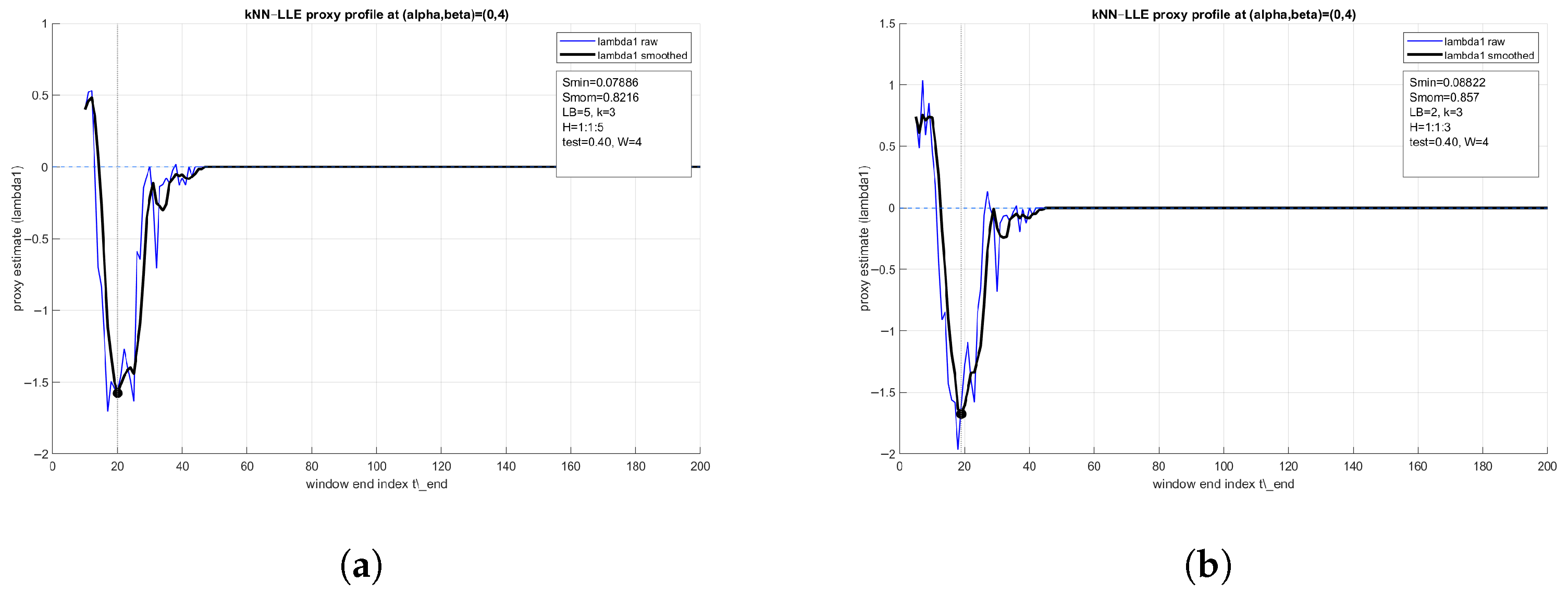
Figure A1 compares the proxy profiles obtained under the baseline profiling configuration and one representative variation. The early negative excursion (contractive transient) and the location of the minimum remain in the same early-iteration region, while the derived scores and change only moderately.
Figure A1.
Illustrative kNN–LLE proxy profiles for under two profiling configurations. Blue: raw proxy estimate . Black: trailing-mean smoothed profile with . The marked minimum is used in computing and . (a) Baseline: LB = 5, H = 1:1:5, , test = 0.40. , , , . (b) Variation: LB = 2, H = 1:1:3, , test = 0.40. , , , .
Appendix A.2. Summary Across the Tested Configurations
Table A1 summarizes the derived scores for all tested configurations in this single-point illustration. Across all settings, the profile exhibits an early minimum (typically in the range –22), and the score values remain in a comparable range, indicating that the observable contractive transient used by and is not an artifact of a single hyperparameter choice for this representative case.
Table A1.
Summary of proxy-profile-derived scores for under multiple profiling configurations.
Appendix A.3. Ranking Robustness on a 30 × 30 Parameter Grid (Heatmap-Level)
To assess robustness at the ranking level, we repeated the sweep on a grid under the baseline profiling configuration and several moderate variations of the profiling hyperparameters. We quantify stability by (i) the Spearman rank correlation between the resulting score landscapes and (ii) the overlap of the top-10 parameter pairs ranked by the score.
Appendix A.3.1. Visualization (Smom Landscapes)
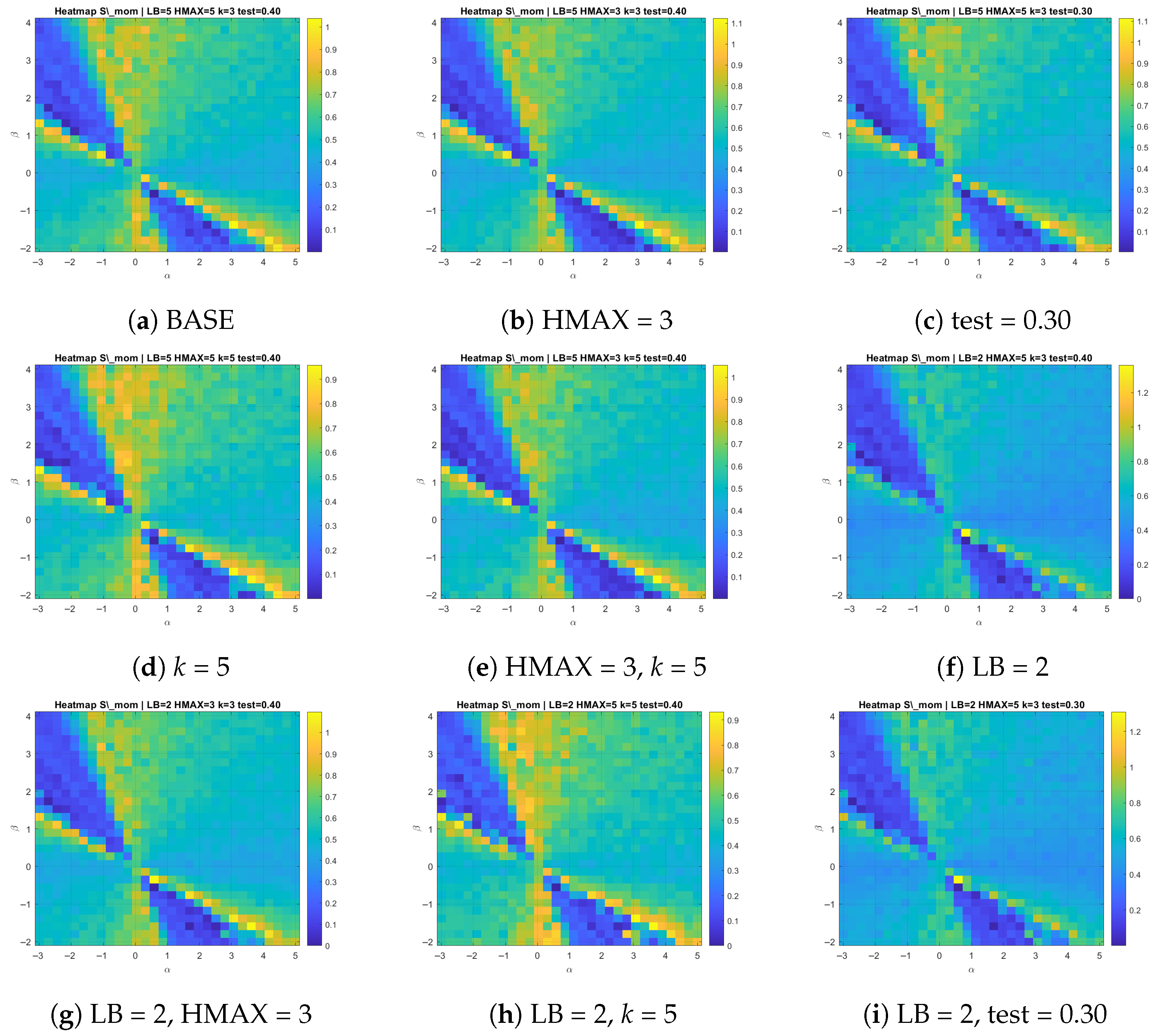
Figure A2 shows the landscapes for the baseline and eight representative variations (one configuration is intentionally omitted for compactness). The high-score corridor remains clearly visible across all shown settings.
Appendix A.3.2. Quantitative Stability Metrics
Table A2 reports Spearman rank correlations and top-10 overlap with the baseline.
Table A2.
Ranking robustness under moderate profiling-hyperparameter changes on a grid (baseline: LB = 5, HMAX = 5, k = 3, test = 0.40).
Figure A2.
Heatmap-level robustness illustration on a grid (only shown for compactness). All panels use the same solver setup and parameter grid; only the profiling hyperparameters are varied, as indicated. Here, BASE denotes the baseline profiling configuration (LB = 5, HMAX = 5, k = 3, test = 0.40).
Appendix A.3.3. Discussion
Overall, the stability results are positive. The landscape remains highly consistent across all tested variations (Spearman –), and the Top-10 overlap stays moderate to high (typically 5–8 common parameter pairs), indicating that the high-score corridor is not an artifact of a single profiling configuration.
Among the tested hyperparameters, reducing the horizon range (HMAX: 5 → 3) and changing the train/test split (test: 0.40 → 0.30) have the smallest impact on the ranking, while decreasing the look-back length (LB: 5 → 2) has the largest effect, especially on . This behavior is expected: depends strongly on the exact location and depth of the profile minimum, so small shifts in can reorder close candidates, whereas aggregates the negative “mass” of the profile and is therefore more robust to minor local shifts.
These findings support the use of the proposed profiling pipeline for practical parameter screening: the identified high-score corridor is stable under moderate changes of the key profiling hyperparameters, and the overall ranking structure is primarily governed by intrinsic contractivity properties of the underlying solver dynamics rather than by tuning artifacts of the profiling configuration.
References
- Gao, Y.; Yang, X.M. Properties of the nonlinear scalar functional and its applications to vector optimization problems. J. Glob. Optim. 2019, 73, 869–889. [Google Scholar] [CrossRef] [Scilit]
- Agrawal, A.; Verschueren, R.; Diamond, S.; Boyd, S. A rewriting system for convex optimization problems. J. Control Decis. 2018, 5, 42–60. [Google Scholar] [CrossRef] [Scilit]
- Gautier, A.; Tudisco, F.; Hein, M. Nonlinear Perron–Frobenius Theorems for Nonnegative Tensors. SIAM Rev. 2023, 65, 495–536. [Google Scholar] [CrossRef] [Scilit]
- Gamal, M.; Zaky, M.A.; El-Kady, M.; Abdelhakem, M. Chebyshev polynomial derivative-based spectral tau approach for solving high-order differential equations. Comput. Appl. Math. 2024, 43, 412. [Google Scholar] [CrossRef] [Scilit]
- Varona, J.L. Graphic and numerical comparison between iterative methods. Math. Intell. 2002, 24, 37–47. [Google Scholar] [CrossRef] [Scilit]
- Jiang, Y.; Liu, H.; Ni, T.; Zhang, K. Inverse problems for nonlinear progressive waves. arXiv 2023, arXiv:2308.07808. [Google Scholar] [CrossRef] [Scilit]
- Stetter, H.J. Analysis of Discretization Methods for Ordinary Differential Equations; Springer: Berlin/Heidelberg, Germany, 1973. [Google Scholar] [CrossRef] [Scilit]
- Bhat, I.A.; Mishra, L.N.; Mishra, V.N.; Tunç, C. Analysis of efficient discretization technique for nonlinear integral equations of Hammerstein type. Int. J. Numer. Methods Heat Fluid Flow 2024, 34, 4257–4280. [Google Scholar] [CrossRef] [Scilit]
- Ortega, J.M.; Rheinboldt, W.C. Iterative Solution of Nonlinear Equations in Several Variables; Academic Press: New York, NY, USA, 1970. [Google Scholar] [CrossRef] [Scilit]
- Noor, K.I.; Noor, M.A. Predictor–corrector Halley method for nonlinear equations. Appl. Math. Comput. 2007, 188, 1587–1591. [Google Scholar] [CrossRef] [Scilit]
- Gutiérrez, J.M.; Galilea, V. Two dynamic remarks on the Chebyshev–Halley family of iterative methods for solving nonlinear equations. Axioms 2023, 12, 1114. [Google Scholar] [CrossRef] [Scilit]
- Weierstraß, K. Neuer Beweis des Satzes, dass jede ganze rationale Funktion einer Veränderlichen dargestellt werden kann als ein Produkt aus linearen Funktionen derselben Veränderlichen. Ges. Werke 1903, 3, 251–269. [Google Scholar] [CrossRef] [Scilit]
- Atanassova, L.; Kyurkchiev, N.; Yamamoto, T. Methods for Computing All Roots of a Polynomial Simultaneously—Known Results and Open Problems; Computing Supplementa; Springer: Vienna, Austria, 2002; Volume 16, pp. 23–42. [Google Scholar] [CrossRef] [Scilit]
- Brari, Z.; Belghith, S. A new algorithm for largest Lyapunov exponent determination for noisy chaotic signals with application to EEG analysis. Chaos Solitons Fractals 2022, 165, 112757. [Google Scholar] [CrossRef] [Scilit]
- Magreñán, Á.A. A new tool to study real dynamics: The convergence plane. Appl. Math. Comput. 2014, 248, 215–224. [Google Scholar] [CrossRef] [Scilit]
- Kyurkchiev, N. Initial Approximations and Root Finding Methods; Wiley–VCH: Berlin, Germany, 1998. [Google Scholar] [CrossRef] [Scilit]
- Chicharro, F.I.; Cordero, A.; Torregrosa, J.R. Drawing dynamical and parameter planes of iterative families and methods. Sci. World J. 2013, 2013, 780153. [Google Scholar] [CrossRef] [Scilit] [PubMed]
- Rockwood, M.P.; Loiselle, T.; Green, M.A. Practical concerns of implementing finite-time Lyapunov exponent analysis with under-resolved data. Exp. Fluids 2019, 60, 74. [Google Scholar] [CrossRef] [Scilit]
- Clauss, P.; Loechner, V. Parametric analysis of polyhedral iteration spaces. J. VLSI Signal Process. Syst. Signal Image Video Technol. 1998, 19, 179–194. [Google Scholar] [CrossRef] [Scilit]
- Shams, M.; Carpentieri, B. Chaos in inverse parallel schemes for solving nonlinear engineering models. Mathematics 2024, 13, 67. [Google Scholar] [CrossRef] [Scilit]
- Varga, R.S. Iterative Analysis; Springer: New York, NY, USA, 1962. [Google Scholar] [CrossRef] [Scilit]
- Velichko, A.; Belyaev, M.; Boriskov, P. A novel approach for estimating largest Lyapunov exponents in one-dimensional chaotic time series using machine learning. Chaos 2025, 35, 101101. [Google Scholar] [CrossRef] [Scilit]
- Ma, Z.S.; Li, X.; He, M.X.; Jia, S.; Yin, Q.; Ding, Q. Recent advances in data-driven dynamics and control. Int. J. Dyn. Control 2020, 8, 1200–1221. [Google Scholar] [CrossRef] [Scilit]
- Shams, M. Theoretical advances in two-step iterative schemes for nonlinear problems. Trans. Comput. Model. Intell. Syst. 2025, 1, 10011. [Google Scholar] [CrossRef] [Scilit]
- Korzun, D.; Meigal, A. Multi-source data sensing in mobile personalized healthcare systems: Semantic linking and data mining. In Proceedings of the 24th Conference of Open Innovations Association (FRUCT); IEEE: New York, NY, USA, 2019; pp. 187–192. [Google Scholar] [CrossRef] [Scilit]
- Rosenblatt, M.; Timmer, J.; Kaschek, D. Customized steady-state constraints for parameter estimation in non-linear ordinary differential equation models. Front. Cell Dev. Biol. 2016, 4, 41. [Google Scholar] [CrossRef] [Scilit]
- Kariya, Y.; Honma, M.; Tokuda, K.; Konagaya, A.; Suzuki, H. Utility of constraints reflecting system stability on analyses for biological models. PLoS Comput. Biol. 2022, 18, e1010441. [Google Scholar] [CrossRef] [Scilit]
- Peñas, D.; González, P.; Egea, J.; Doallo, R.; Banga, J. Parameter estimation in large-scale systems biology models: A parallel and self-adaptive cooperative strategy. BMC Bioinform. 2017, 18, 52. [Google Scholar] [CrossRef] [Scilit]
- Beltrão, G.; Martins, W.; Alaee-Kerahroodi, M.; Schroeder, U.; Tatarinov, D. Adaptive nonlinear least squares framework for contactless vital sign monitoring. IEEE Trans. Microw. Theory Tech. 2023, 71, 1696–1710. [Google Scholar] [CrossRef] [Scilit]
- Shams, M.; Velichko, A.; Carpentieri, B. Direct finite-time contraction (step-log) profiling–driven optimization of parallel schemes for nonlinear problems on multicore architectures. arXiv 2026, arXiv:2601.13637. [Google Scholar] [CrossRef] [Scilit]
- Rosen, M.I. Niels Hendrik Abel and equations of the fifth degree. Am. Math. Mon. 1995, 102, 495–505. [Google Scholar] [CrossRef] [Scilit]
- Papp, D. Semi-infinite programming using high-degree polynomial interpolants and semidefinite programming. SIAM J. Optim. 2017, 27, 1858–1879. [Google Scholar] [CrossRef] [Scilit]
- Reinke, B.; Schleicher, D.; Stoll, M. The Weierstrass–Durand–Kerner root finder is not generally convergent. Math. Comput. 2023, 92, 839–866. [Google Scholar] [CrossRef] [Scilit]
- Anourein, A.W.M. An improvement on two iteration methods for simultaneous determination of the zeros of a polynomial. Int. J. Comput. Math. 1977, 6, 241–252. [Google Scholar] [CrossRef] [Scilit]
- Zhang, X.; Peng, H.; Hu, G. A high order iteration formula for the simultaneous inclusion of polynomial zeros. Appl. Math. Comput. 2006, 179, 545–552. [Google Scholar] [CrossRef] [Scilit]
- Cordero, A.; Torregrosa, J.R.; Triguero-Navarro, P. Jacobian-free vectorial iterative scheme to find simple several solutions simultaneously. Math. Methods Appl. Sci. 2025, 48, 5718–5730. [Google Scholar] [CrossRef] [Scilit]
- Zeng, Z. Computing multiple roots of inexact polynomials. Math. Comput. 2005, 74, 869–903. [Google Scholar] [CrossRef] [Scilit]
- Nedzhibov, G. Dynamic mode decomposition via polynomial root-finding methods. Mathematics 2025, 13, 709. [Google Scholar] [CrossRef] [Scilit]
- Proinov, P.D.; Petkova, M.D. A new semilocal convergence theorem for the Weierstrass method for finding zeros of a polynomial simultaneously. J. Complex. 2014, 30, 366–380. [Google Scholar] [CrossRef] [Scilit]
- Shams, M.; Kausar, N.; Samaniego, C.; Agarwal, P.; Ahmed, S.F.; Momani, S. On efficient fractional Caputo-type simultaneous scheme for finding all roots of polynomial equations with biomedical engineering applications. Fractals 2023, 31, 2340075. [Google Scholar] [CrossRef] [Scilit]
- Shams, M. On a stable multiplicative calculus-based hybrid parallel scheme for nonlinear equations. Mathematics 2024, 12, 3501. [Google Scholar] [CrossRef] [Scilit]
- Machado, R.N.; Lopes, L.G. A family of Ehrlich-type accelerated methods with King’s correction for the simultaneous approximation of polynomial complex zeros. Glob. J. Pure Appl. Math. 2019, 15, 789–802. [Google Scholar]
- Petković, M.S.; Petković, L.D.; Džunić, J. On an efficient method for the simultaneous approximation of polynomial multiple roots. Appl. Anal. Discrete Math. 2014, 8, 73–94. [Google Scholar] [CrossRef] [Scilit]
- Egbo, M.K. A fundamental review on composite materials and some of their applications in biomedical engineering. J. King Saud Univ.-Eng. Sci. 2021, 33, 557–568. [Google Scholar] [CrossRef] [Scilit]
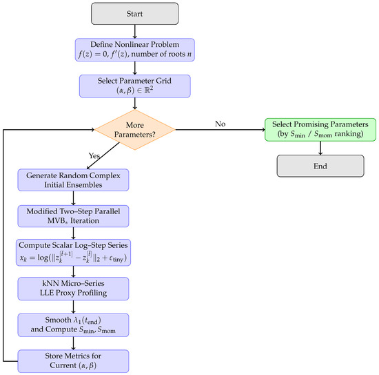
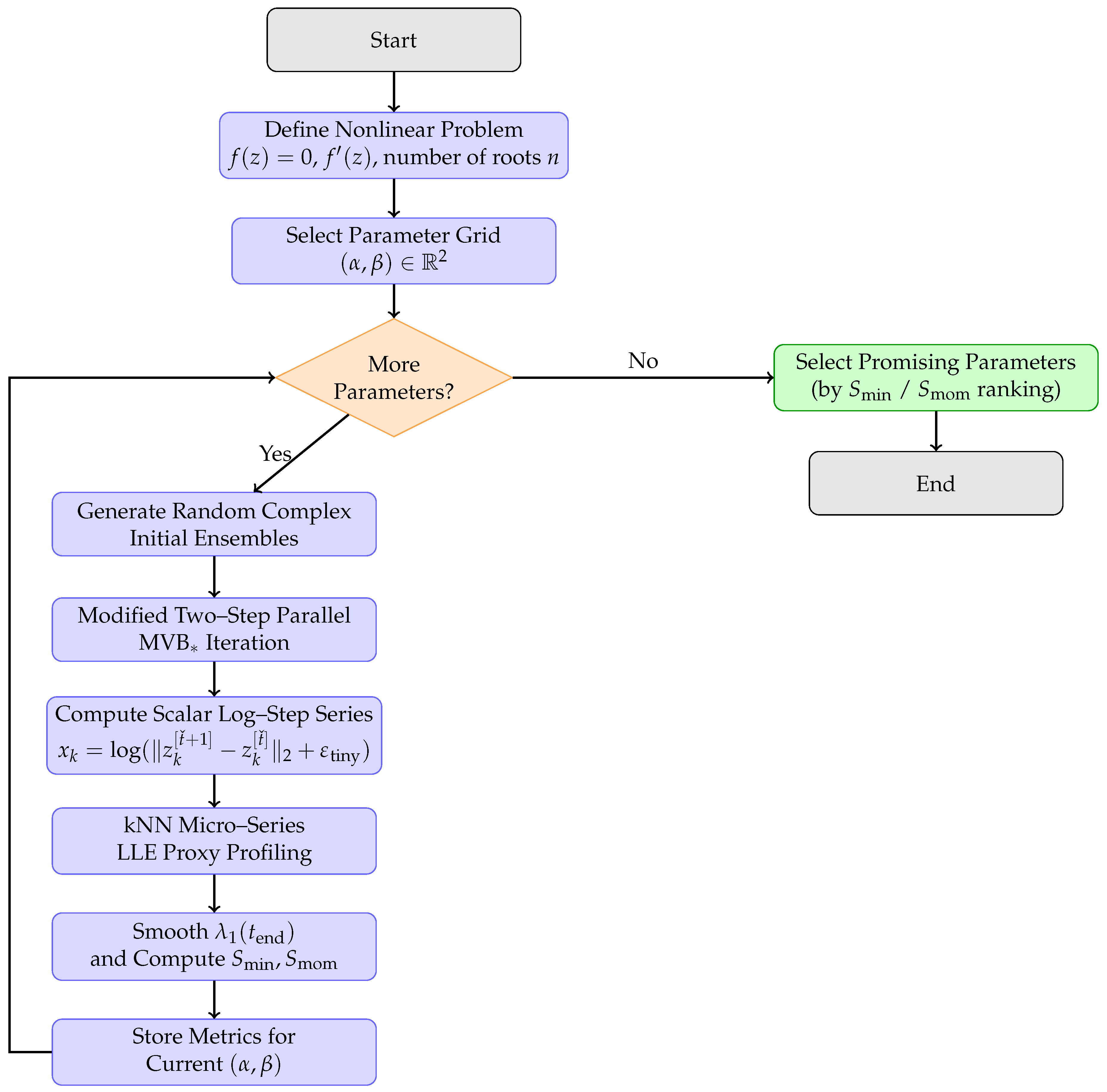
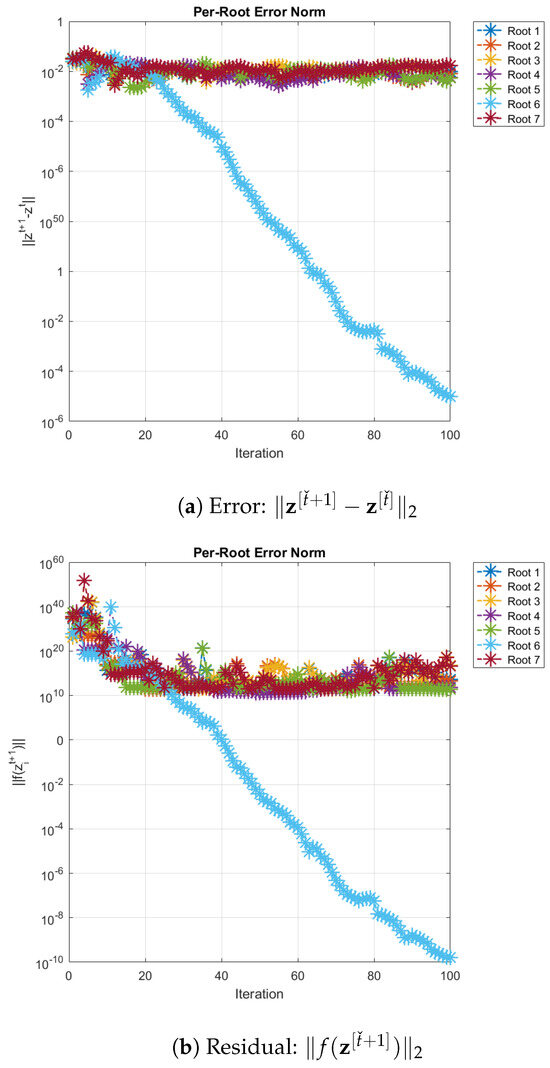
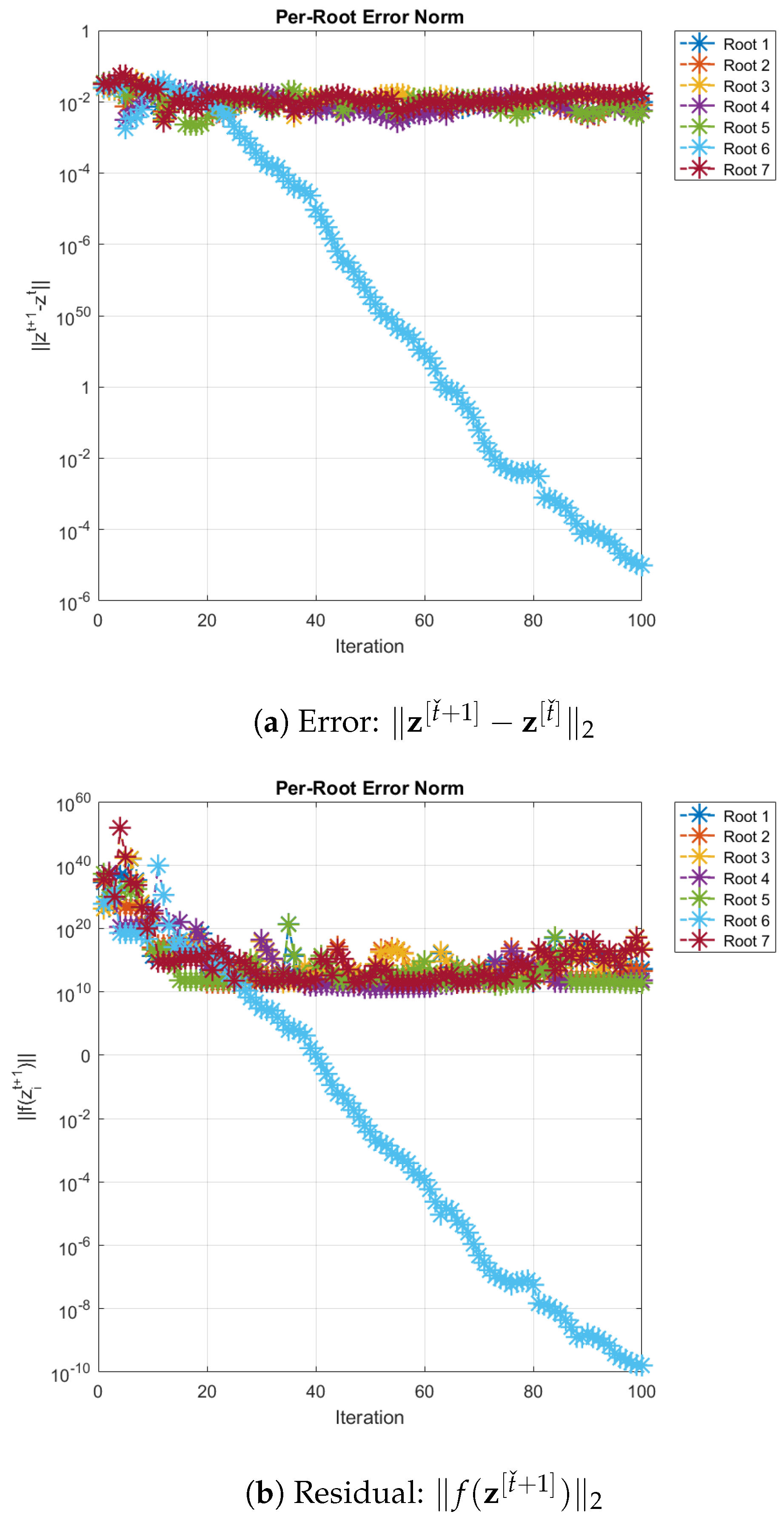
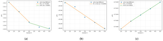
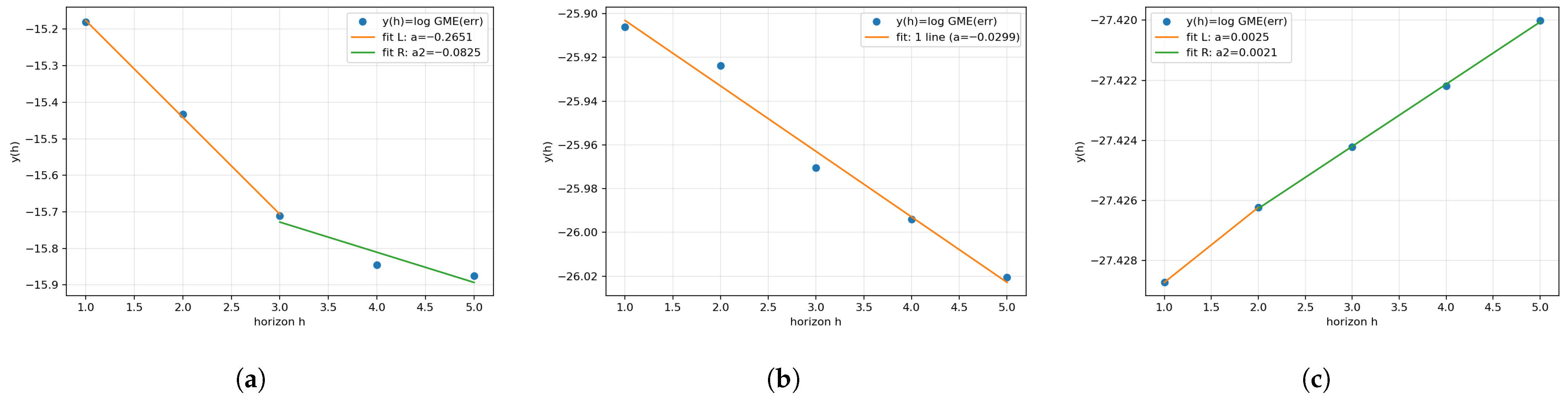
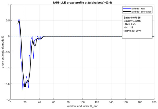
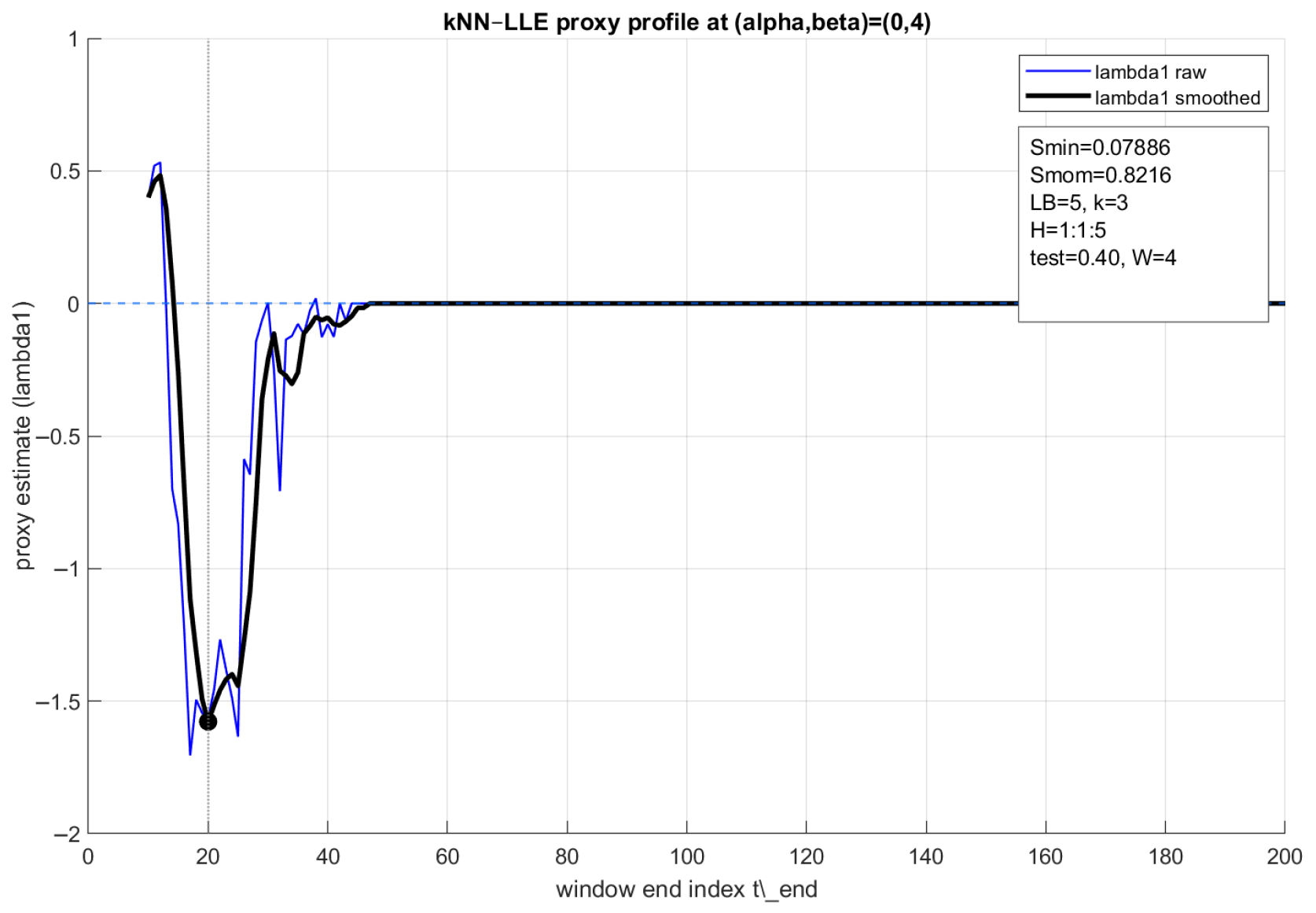
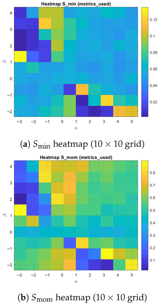
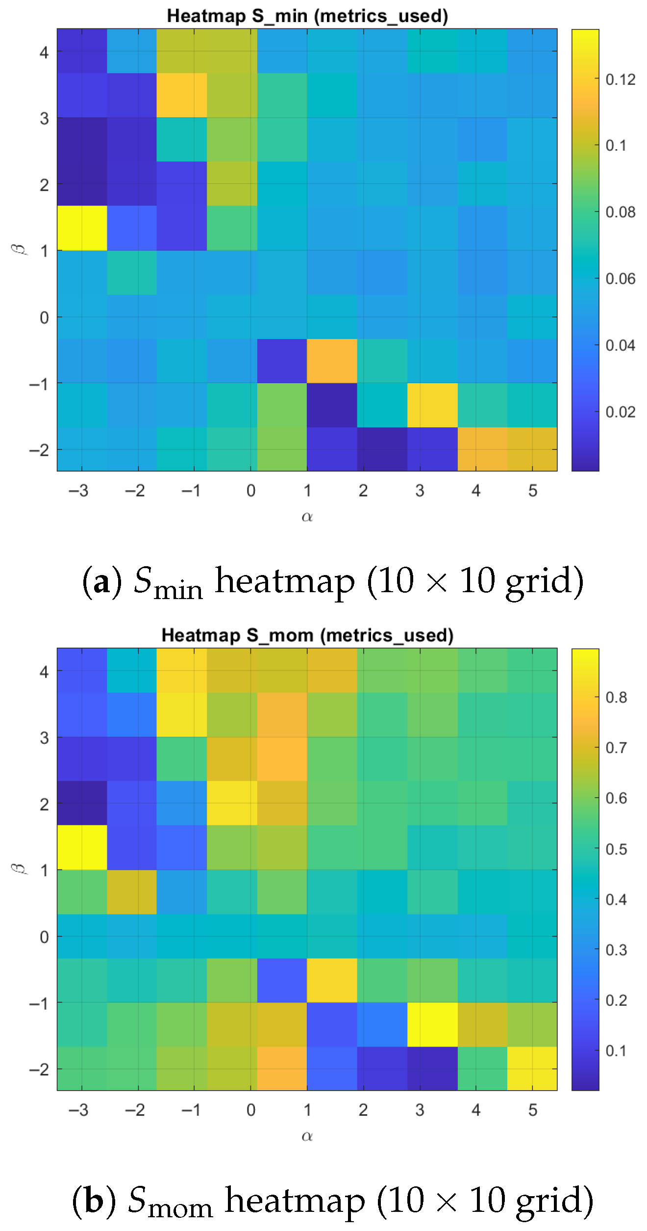
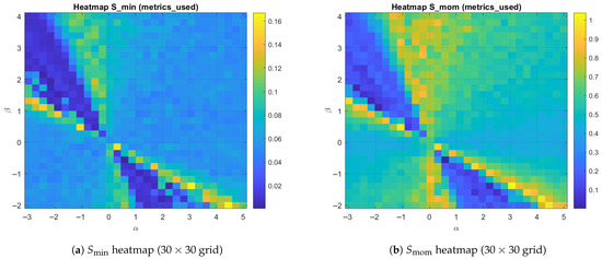
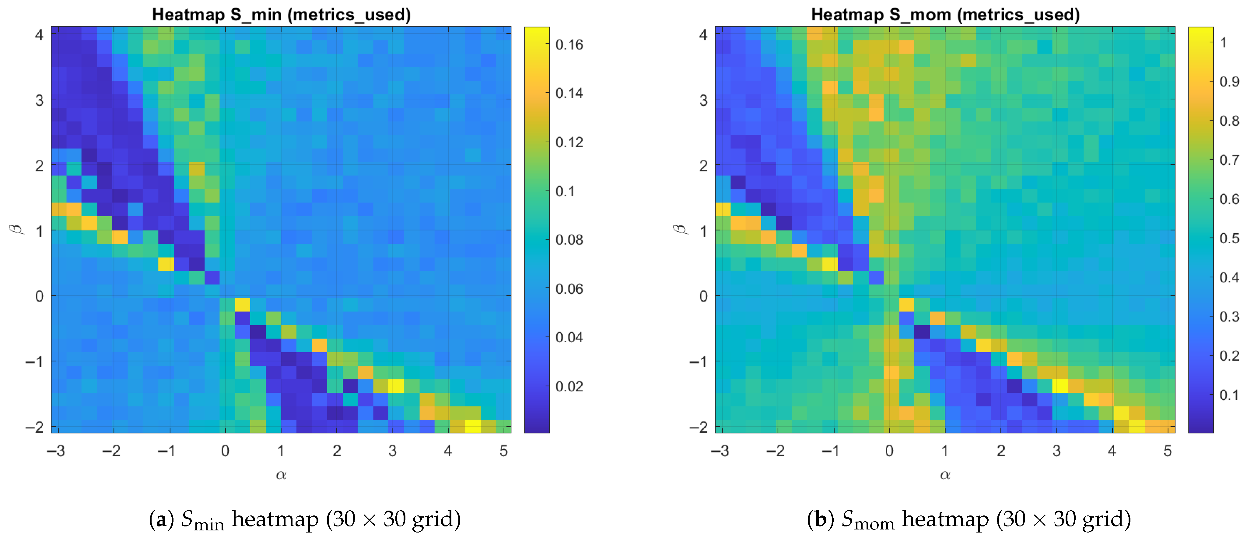
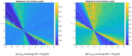
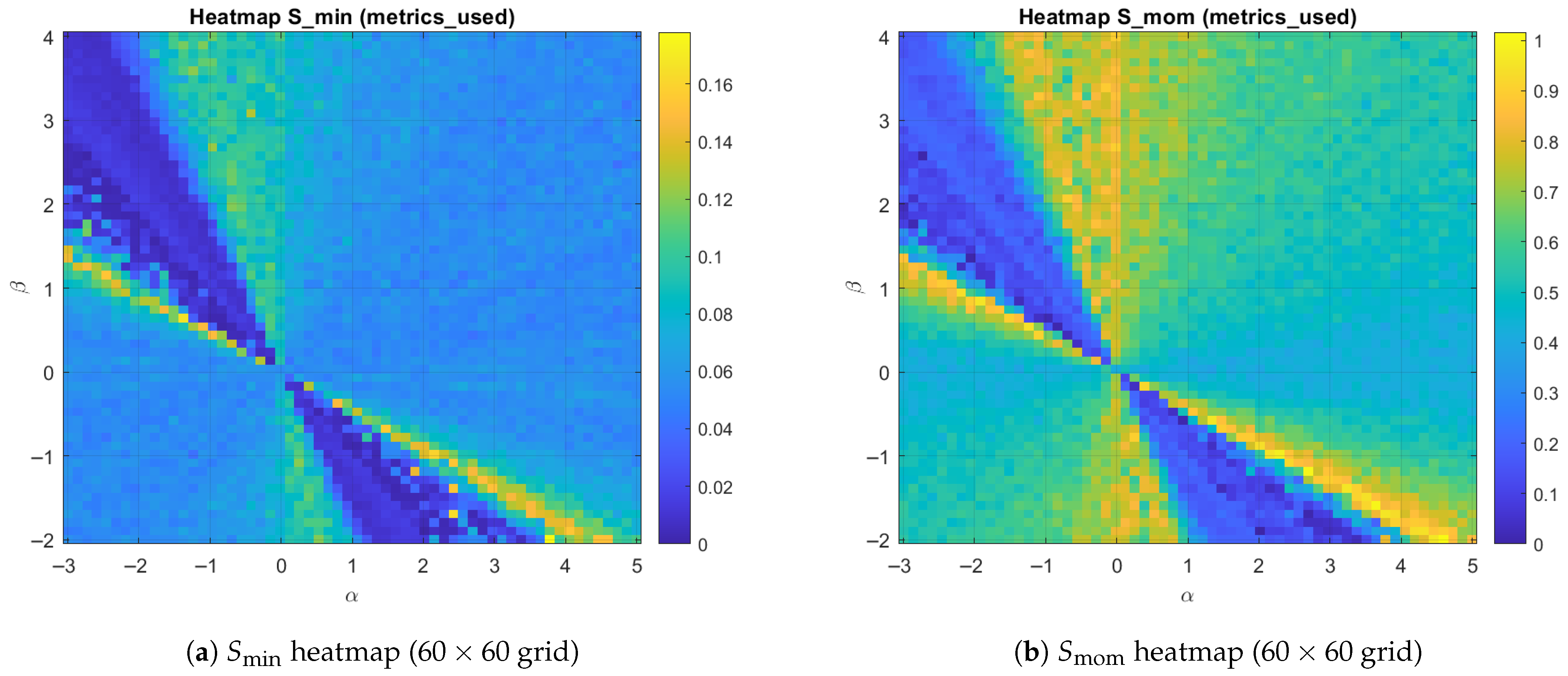
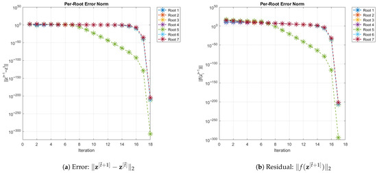
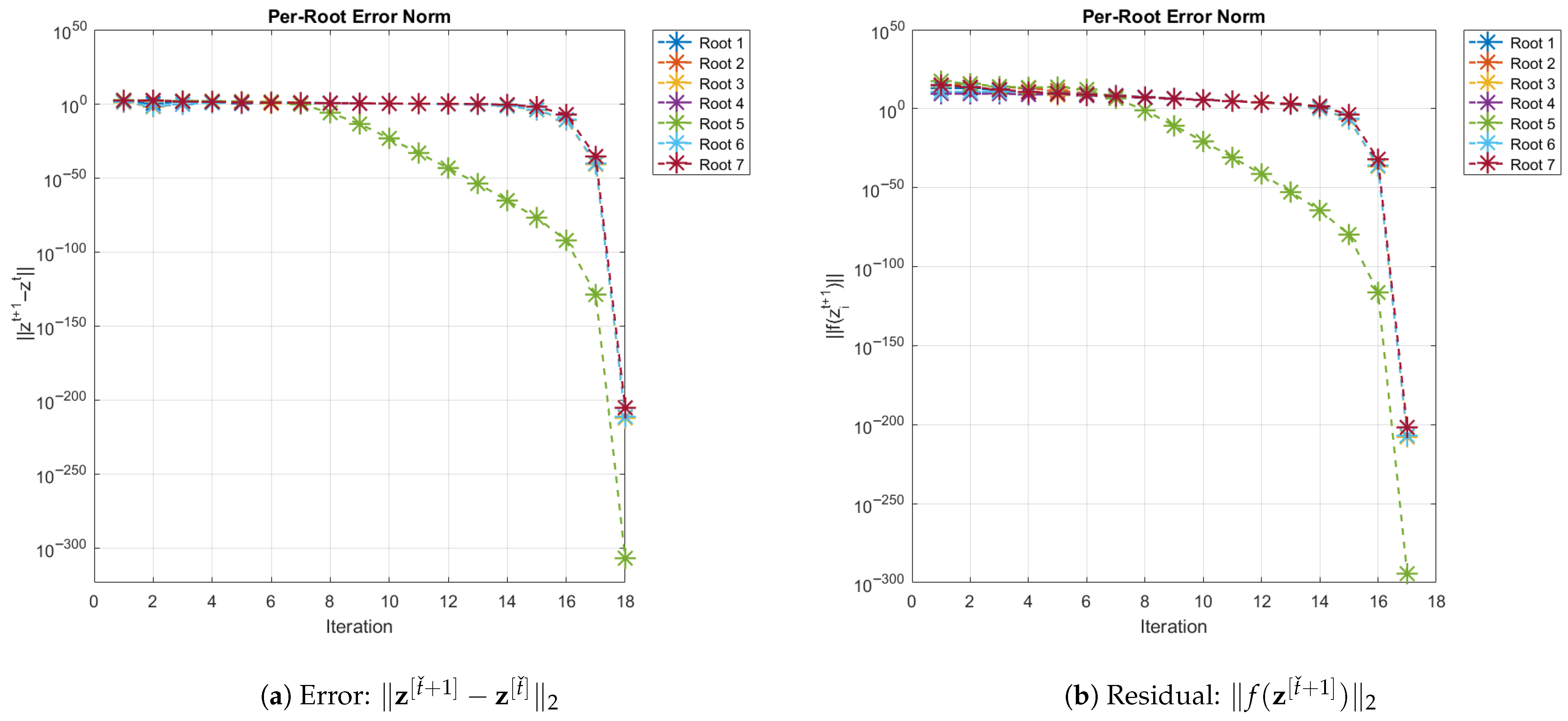

Disclaimer/Publisher’s Note: The statements, opinions and data contained in all publications are solely those of the individual author(s) and contributor(s) and not of MDPI and/or the editor(s). MDPI and/or the editor(s) disclaim responsibility for any injury to people or property resulting from any ideas, methods, instructions or products referred to in the content. |
© 2026 by the authors. Licensee MDPI, Basel, Switzerland. This article is an open access article distributed under the terms and conditions of the Creative Commons Attribution (CC BY) license.