


Abstract
In volatile global political and economic shifts, High-Impact Political and Economic Statements (HIPES) by influential leaders often trigger immediate market panic and sharp fluctuations in economic indicators. The forecasting of these indicators is critical for informed decision-making. This study addresses the challenge of enhancing Large Language Models’ (LLMs’) forecasting performance by integrating academic theories as optimization variables, which guide LLMs to analyze HIPES, map relevant academic theories, and convert them into optimization variables, while equipping LLMs with scholars’ diverse perspectives on academic theories. Using Gemini Pro 3, we developed a Dual-Path Comparative Framework: one path employs Direct Forecast (named as F1) based solely on HIPES, while the other combines HIPES with mapped Optimization Variables (named as F2). Both paths were experimented to forecast 75 International Economic Indicators across five asset categories. Results show F2 significantly outperforms F1 in overall accuracy in volatile assets (e.g., crypto), while F1 favors relatively stable asset classes (e.g., commodities). These findings address gaps in “Theory-Guided AI” research, providing strategies for asset-specific forecasting.
Keywords:
Large Language Models (LLM); political and economic statements; economic forecasting; theory-guided AI applications; technical analysis indicators MSC:
68T20; 68T37; 68T50; 91B82
1. Introduction
In today’s globalized economy, high-impact political and economic statements (hereafter, referred to as HIPES) often trigger abrupt market volatility, even when unrelated to explicit policy changes. Geopolitical rhetoric, such as military declarations (e.g., military exercise declarations preceding the Ukraine–Russia conflict) or shifts in trade policies (e.g., U.S.-China technology and trade war policies), can rapidly destabilize capital markets, posing challenges for stakeholders seeking timely, data-driven decisions [1]. Traditional econometric models, reliant on historical numerical indicators, struggle to capture nonlinear market sentiment or causal relationships embedded in unstructured political discourse. Generative AI and Large Language Models (LLMs) offer transformative potential by enabling semantic analysis of non-structured texts, allowing direct interpretation of political and economic sentiment [2]. However, their accuracy in forecasting high-complexity HIPES is subject to considerable challenges, remaining underexplored, particularly regarding their influence on international economic indicators (IEIs) like exchange rates and cryptocurrencies. Existing studies predominantly employ an end-to-end Direct Forecast (namely, F1) model, which passively generates numerical outputs from raw text without exposing inference pathways. This black-box approach limits practical applicability and causal transparency. To address this gap, this research presents an innovative mechanism, referred to as the Academic Forecast (namely, F2), optimized by academic theory, through integrating robust causal relationships from academic theories as optimization variables. By structuring LLM inputs with theoretical frameworks, our F2 model aims to enhance the accuracy and stability of economic forecasting by a hybrid approach. We investigate whether F2 outperforms F1 in forecasting accuracy for diverse asset classes, while emphasizing the necessity of theoretical integration to mitigate LLM hallucinations and improve reliability in high-stakes economic scenarios.
Existing studies often input raw transcripts of HIPES into LLMs to generate numerical forecasts for key economic indicators. However, their approach neglects a critical limitation: LLMs, while capable of semantic understanding, may produce unreliable outputs due to divergent reasoning or “hallucination” in the absence of structured guidance. The academic community has yet to explore how to systematically integrate “Academic Theory” as a concrete “Optimization Variable” to refine the forecasting capabilities of LLMs. A key gap lies in the lack of attempts to embed validated causal mechanisms from academic theories—such as the Exchange Rate Overshooting Theory or the Efficient Market Hypothesis—as part of the prompt engineering process. By treating these theories as “Optimization Variables,” the input framework becomes a “navigation map” that channels LLMs toward rigorous economic logic rather than superficial sentiment analysis [3]. Our study addresses this gap by investigating whether incorporating “Academic Theory” as an “Optimization Variable” can enhance the forecasting performance of LLMs when judging market trends through technical indicators. Unlike simplistic Direct Forecast (F1) models, the F2 approach introduces theoretical structure to mitigate hallucinations and improve reliability in high-stakes economic analyses. In sum, this study addresses the research gap by examining two research questions:
RQ1: Does the Academic Forecast model (F2)—incorporating “Academic Theories” as “Optimization Variables”—significantly improve the accuracy and stability of forecasting performance as compared to the Direct Forecast (F1) model?
RQ2: Do asset types (e.g., Commodities Market, Stock Market Indices, Foreign Exchange Rates, Cryptocurrencies, 10-Year Government Bond Yield) demonstrate distinct advantages in forecasting under various models (F1 and F2)?
2. Literature Review with Research Method Elaboration
2.1. High-Impact Political and Economic Statements, Their Market Impacts, and LLMs
High-impact political and economic statements (HIPES)—such as those by influential decision-makers (e.g., heads of major economies, finance ministers) in public forums—are among the central drivers of global financial market volatility. Public narratives spread rapidly, altering economic behavior and market confidence [4]. Quantitative evidence, such as the Economic Policy Uncertainty (EPU) index [5], suggests that political rhetoric or policy debates directly influence investment and output. High-impact statements possess immediate pricing power, and consequently, central bank communication has evolved into a core monetary policy tool [6]. Additionally, U.S. presidents’ tweets on the Federal Reserve significantly influence financial markets, proving that single actors’ speech can disrupt monetary policy and trigger turbulence [7]. At the international level, geopolitical risks are linked to “threat” narratives, escalating risk aversion, and impacting global markets trading commodities and bonds [1]. National risk perceptions diffuse globally via multinational corporate texts [8]. Political risks propagate directly to enterprises, reducing capital spending and hiring [9]. “Regulatory Narratives” on climate policies are identified as critical pricing signals, with firms’ sensitivity reflected in stock and option prices [10]. To capture speech impacts, a financial lexicon linking text tone to asset prices was developed [11]. Machine learning models may outperform traditional linear models in forecasting asset prices, providing technical rationale for LLM-based analysis [12]. Domain-specific LLMs (e.g., FinBERT) can enhance predictive accuracy by interpreting economically relevant text features [13]. This study proposes that publicly released HIPES are an important source for analyzing their market impacts.
Since political and economic statements possess significant market influence, especially with their textual content harboring critical signals for economic trend prediction, financial text analysis has transitioned from traditional “Frequency Statistics” to modern “Semantic Reasoning.” Early approaches relied on the financial sentiment lexicon [11], reducing unstructured text to a “Bag of Words” model for sentiment aggregation. However, it is highlighted that financial data now operates in a “big data” era [14], characterized by volume, variety, and high dimensionality. Traditional econometric methods struggle to capture nonlinear relationships and deep semantics in unstructured texts (e.g., complex policy tones and ambiguous rhetoric), limiting predictive accuracy. The rise of generative AI has revolutionized forecasting. LLMs, exemplified by ChatGPT 4, are confirmed to transcend statistical tools, offering cognitive and reasoning capabilities akin to human experts [15]. This enables LLMs to interpret causal logic and sentiment embedded in HIPES. In this context, integrating unstructured textual sentiment data are demonstrated to significantly enhance stock price forecast accuracy [2]. Given that even high-noise social media comments provide actionable signals, HIPES are expected to exert significant impacts on asset prices. This represents a paradigm shift in financial forecasting, surpassing traditional methodological frameworks. In summary, this study adopts LLMs as the core experimental platform to harness their capacity for semantic reasoning, analysis, and forecasting upon market trends.
While deep learning has demonstrated exceptional performance in economic forecasting, as demonstrated, machine learning models often face the “black box” challenge, lagging behind in interpretability and causal reasoning [12]. It is found that purely data-driven approaches struggle with policy counterfactuals, as high correlations do not equate to valid causality [16]. Since structural shocks like HIPES expose the limitations of models without theoretical constraints, the Theory-Guided Data Science (TGDS) paradigm was proposed [3], advocating for scientific consistency in machine learning frameworks. Given that extant Natural Language Processing (NLP) applications in financial forecasting remain limited to sentiment scoring, ignoring deeper logical chains, LLMs’ superior causal argument generation is highlighted [17], yet the gap persists: no study has fully integrated causal mechanisms with generalization ability into predictive models. This research fills that gap by embedding academic theory as an optimization variable, transforming LLMs from intuitive sentiment forecasting to theory-supported logical reasoning.
2.2. LLMs as Research Tools—Thoughts for Causal Reasoning and Economic Forecasting
Data-driven models face limitations without causal structures to enhance LLM forecasting efficacy, and therefore, this study adopts the TGDS paradigm [3] for prioritizing scientific consistency to construct generalized models. Textual information is emphasized as a rich complement to structured data [18]; LLMs can be used as economic research tools capable of extracting insights from academic theories [19]. By transforming such extracted insights into a causal-effective “Optimization Variable,” LLMs may outperform state-of-the-art algorithms in generating accurate causal arguments [17]. Technically, the “Chain-of-Thought” (CoT) method (e.g., generating intermediate reasoning steps) [20], alongside the zero-shot reasoning mechanism (e.g., the prompt “Let’s think step by step”) [21], can extract structured causal chains from unstructured text. Financial reasoning requires an emergent capacity of complex LLMs for predicting price drifts [22]. These advancements contribute to the integration of neural networks with symbolic reasoning [23]. This study proposes the “Academic Theory-Based Optimization Variables (ATBOVs)”, leveraging HIPES texts and LLMs to extract textual implications and then converting them into structured theoretical knowledge archives. Such archives are then fed back as Optimization Variables to LLMs, aiming to improve forecasting outcomes through theoretical frameworks as compared to pure textual inputs.
The granularity and originality of input data critically influence LLM forecasting outcomes. This study prioritizes HIPES as primary source transcripts, excluding media-processed second-hand news/information. The rationale hinges on two key principles: mitigating “Intermediary Bias” and preserving “Soft Information” integrity. Firstly, the media often distorts or filters information to align with readers’ preexisting beliefs, resulting in a reporting slant [24]. Using journalist-curated news as input risks analyzing filtered perspectives rather than original facts. Direct control over the “Data Generating Process” is suggested, necessitating direct access to decision-makers’ original statements to avoid third-party noise [25]. Secondly, while hard data are easily transmissible, soft information (e.g., tone, hesitation, confidence levels) is inseparable from speakers and prone to loss during relaying [26]. Manager-specific tone holds unique predictive power, explaining performance beyond financial reports [27]. Similarly, national leaders’ speech tone implicitly signals policy commitment strength. This study argues that only primary transcripts analyzed via LLMs can accurately capture these subtle, market-influencing signals.
In politically and economically narrative-driven forecasting, LLM input data and timeline design must adapt to rapidly evolving information environments. Historical data’s value in forecasting attenuates over time, limiting its relevance to current HIPES. To capture short-term dynamics, this study excludes long-term data, focusing instead on speech transcripts from “Experiment Day” to “30 days prior” as input. A rolling window strategy is employed, grounded in structural break analysis. Pre-break historical data introduces estimation bias, thus making our study favor the prompt of “discard distant, prioritize recent” approach [28], which not only ensures the model reflects current market logic but also reduces sample size and minimizes Mean Squared Forecast Error. In volatile economic environments, prioritizing immediate information accuracy over long-term samples is indeed an optimal strategy. Additionally, rolling windows assign a higher weight to recent data, enhancing sensitivity to trend changes in unstable time series [29]. Inspired by the single-step-ahead (T + 1) framework, which is used to simulate investor strategies based on post-market close [30], this study employs two-time windows: “forecasting 1 day ahead (T + 1)” for immediate market reactions and “forecasting 7 days ahead (T + 7)” for post-digestion price adjustments. Daily rolling updates allow dynamic sensitivity adjustments to political and economic shocks, improving the robustness and credibility of experimental outcomes.
2.3. Comparison of Forecasting Models, F1 and F2
Proposing ATBOV for market trend via economic indicators, this study defines objective benchmarks and evaluation metrics for accuracy testing and performance comparison against our forecasting models. Close-market prices/indexes/averages of widely used technical indicators can be used as the “Realized Volatility” benchmark [31]. In this study, comparing forecasting models involves analyzing differences in loss functions, such as MSE and QLIKE, to ensure forecast ranking accuracy despite noisy volatility proxies [32]. To quantify marginal contributions of ATBOV (i.e., the academic theory-based optimization variable), the out-of-sample performance metric is suggested as a core indicator [33]. These metrics measure predictive error reduction relative to the benchmark, directly reflecting performance gains. This study uses these metrics to confirm that theory-optimized variables enhance predictive accuracy and translate statistical precision into substantive economic gains [34]. Consequently, duly designed experiments can validate the substantive forecast value of ATBOV through numerical accuracy comparisons, asset win rate counts, and statistical analysis of performance distribution.
Numerical differences between our forecasting models (F1 and F2) alone are insufficient to conclude significance; rigorous statistical validation is required. In predictive accuracy testing, the “DM test” was introduced by Diebold and Mariano as the gold standard for assessing significant differences in predictive errors [35], and their work was extended by Clark and West with the “CW test” for nested models, addressing parameter noise in large-scale models [36]. Recent generative AI studies followed this paradigm, confirming LLMs’ predictive superiority over traditional models and validating AI ratings’ association with returns via correlation tests [37,38]. This study adopts the “Paired Samples t-test” to evaluate the gains in forecasting performance from introducing the ATBOV. By treating the prediction accuracy error as a pair of samples, it calculates the difference in the loss function between F1 and F2 at each time point and tests whether the mean difference is statistically significant. This approach aligns with the DM test’s rigor, ensuring robust validation of the optimization variable’s forecasting value.
2.4. Current Limitations of LLMs in Economic Forecasting
While LLMs demonstrate considerable promise in forecasting, prior research [39] highlights critical limitations in economic applications, particularly regarding noise sensitivity, financial knowledge gaps, and weak causal reasoning. In response, this study proposes an original framework based on the following trajectory: (HIPES Context → Academic Theory → Optimization Variable → Assisted Forecasting → Convergence of Predictions → Minimization of Predictive Hallucinations). Existing literature lacks similar conceptual frameworks. This study utilizes a controlled comparison between Direct Prediction (F1) and Theory-Informed Prediction (F2). This approach aims to rectify data sensitivity and logical deficiencies, effectively suppressing stochastic divergence to improve the robustness and logical consistency of economic forecasting within complex, real-world environments.
2.5. Recap of Research Method Elaboration
This study elaborates on a forecasting initiative, the Academic Theory-Based AI Forecasting Initiative, to transform unstructured text into economic indicators, and the initiative comprises four stages as follows.
- Stage 1, Signal Purification, excludes secondary media, focusing solely on first-hand transcripts of HIPES from the 30 days prior to forecasting.
- Stage 2, Theoretical Injection, integrates the ATBOV into LLMs, embedding rigorous causal logic from academic theories to enable theory-supported logical inference.
- Stage 3, Dynamic Forecasting and Dual-Mode Testing, employs a Rolling Window mechanism to capture short- and medium-term market dynamics, comparing F1 and F2 models under the (T + 1)-time window and (T + 7)-time window.
- Stage 4, Validation of Forecasting Gains, involves numerical comparisons of accuracy and performance, followed by statistical significance tests to confirm substantive improvements from academic theory integration.
3. Research Methodology and Experiment Design
3.1. Research Framework
3.1.1. Seventy-Five International Economic Indicators Across Five Asset Categories
To assess cross-asset generalization, this study employs 75 International Economic Indicators (IEIs), categorized into five groups—Commodities (Commodities); Stock Indices (Indices); Foreign Exchange Rates (Exchange Rates); Cryptocurrencies (Crypto); and 10-Year Government Bond Yields (10Y Yield)—each comprising 15 indicators (Table 1). The Realized Value (RV), defined as the Close Price obtained from tradingeconomics.com, is employed in subsequent calculations. Based on inputs, the framework establishes an objective benchmark for the Forecast Estimate Index (FEI) series through accuracy assessment with the FEI metric, performance comparison via Diff. values, credibility validation using paired sample t-tests, and volatility analysis of 75 IEIs, forming the basis for empirical analysis.
Table 1.
Approximately 75 International Economic Indicators (IEIs) Across Five Asset Categories.
3.1.2. Research Framework of the Dual-Path Comparative Experiment
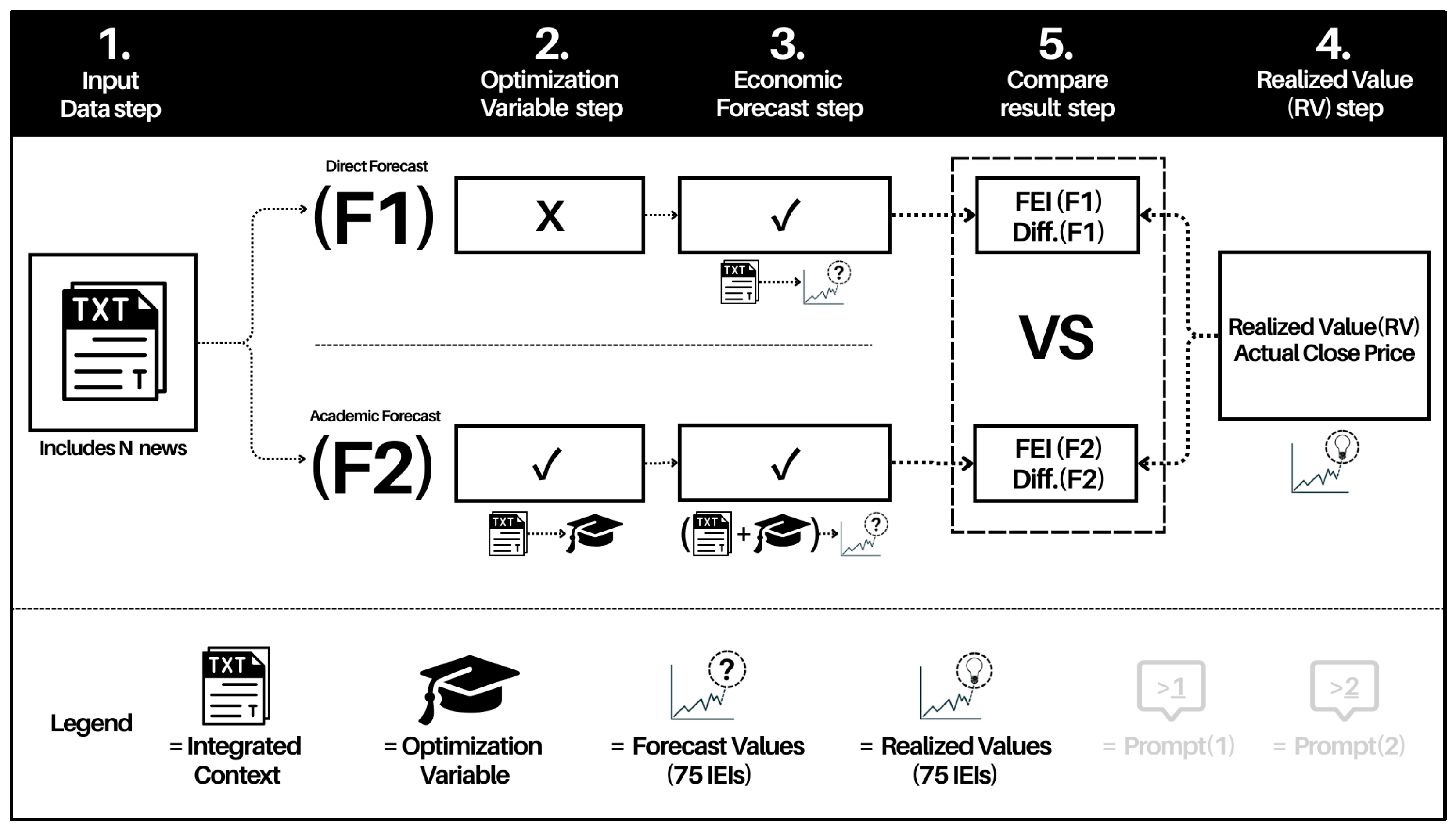
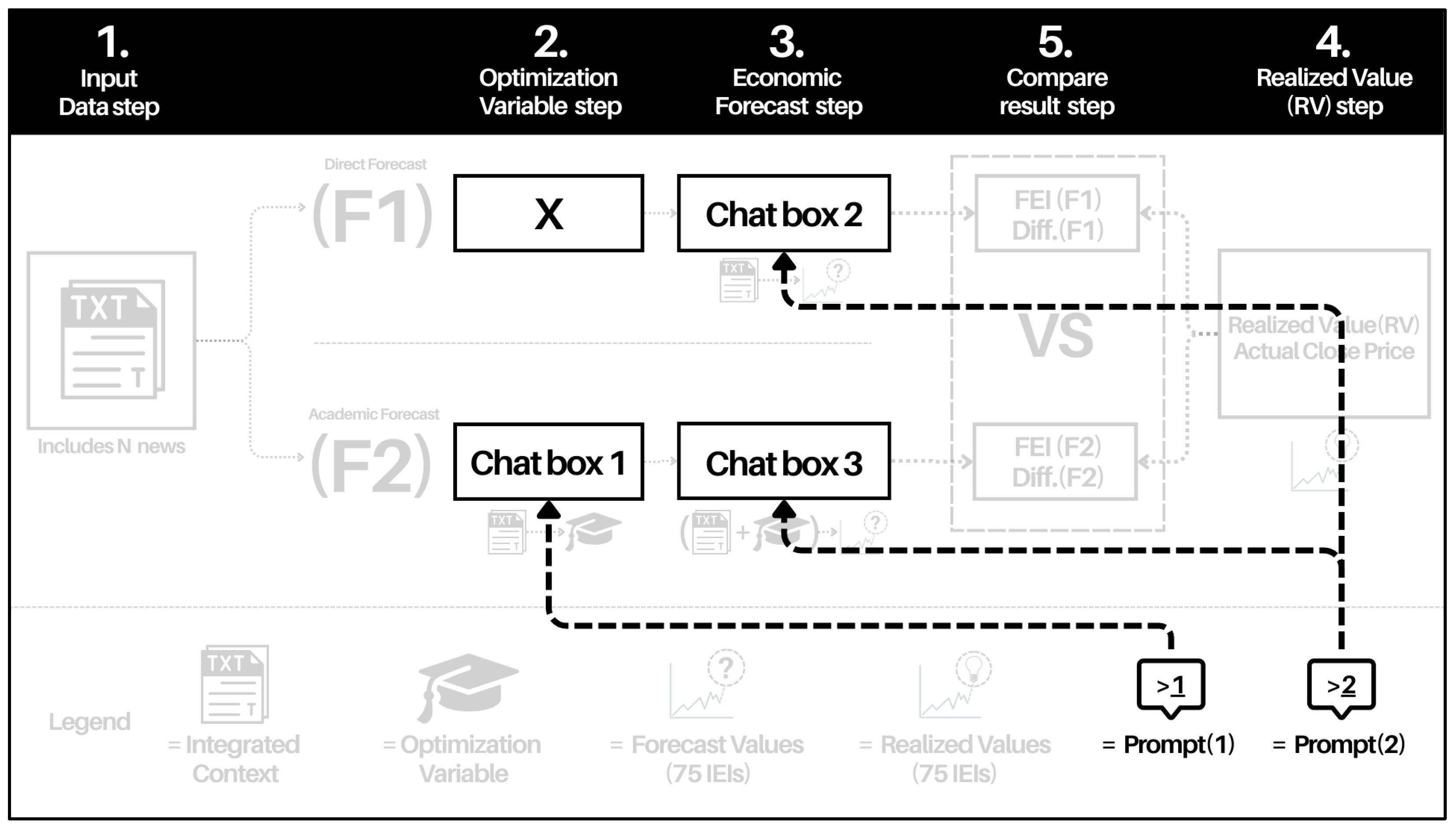
The proposed experimental framework evaluates whether integrating “Academic Theory” into the “Optimization Variable” enhances LLMs’ forecasting accuracy and performance. A rigorous “Dual-Path Comparative Framework” is constructed to compare the control group (F1) and experimental group (F2). The process, illustrated in Figure 1, comprises five steps:
Figure 1.
Research Framework of the Dual-Path Comparative Experiment.
- Input Data Step:For each forecasting day, the system aggregates 30 days of news (representing HIPES) to form an Integrated Context, which is input into the LLM. This ensures both groups operate under identical input conditions.
- Optimization Variable Step:Direct Forecast (F1) skips the Academic Theory extraction process, while Academic Forecast F2 generates an Optimization Variable by inferring academic theories from the Integrated Context and storing them as textual data.
- Economic Forecast Step:Both F1 and F2 forecast the closing prices of 75 IEIs. F1 relies solely on the Integrated Context to generate forecasts, while F2 integrates the Optimization Variable to refine forecasts through academic theory.
- Realized Value (RV) Step:Actual closing prices of the 75 indicators are extracted as the Realized Value (RV) on the target day.
- Compare Result Step:Forecast accuracy and performance are evaluated through the FEI series, Diff. values, paired sample t-tests, and asset volatility, establishing an objective benchmark based on 75 IEIs. This analysis determines whether F2 significantly outperforms F1 and highlights broader trends to extend the study’s practical relevance.
3.1.3. Workflow of the Prompt-Guided Independent Inference Processes
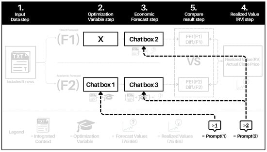
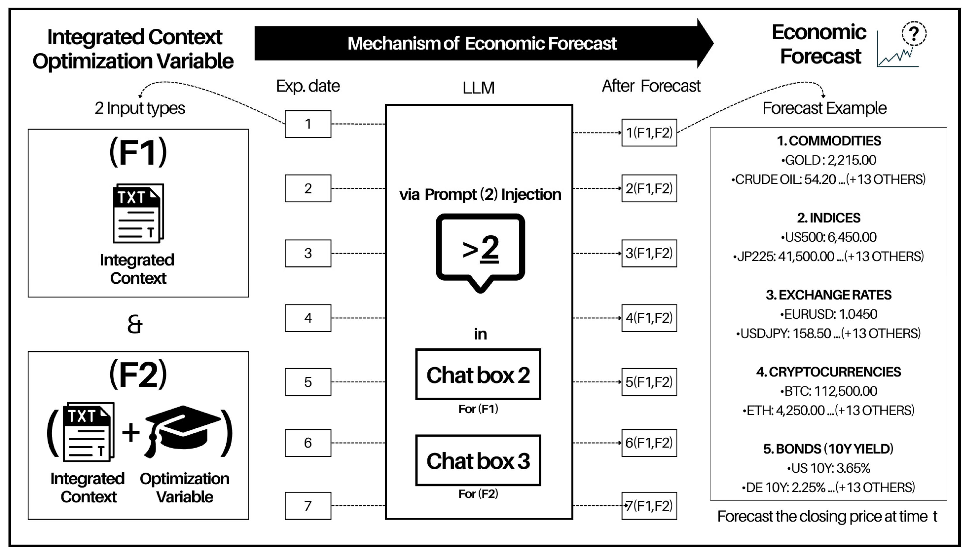
This experiment uses three non-interfering LLM chat windows (see Figure 2): Chat Box 1 generates Optimization Variables with Academic Theory via Prompt (1) for F2. Chat Boxes 2 and 3 employ Prompt (2) for numerical forecasting, with Chat Box 2 assigned to F1 and Chat Box 3 to F2. This setup ensures no interference between identical chat windows.
Figure 2.
Workflow of the Prompt-Guided Independent Inference Sessions.
3.1.4. Functional Specification of Prompt (1) and Prompt (2)
This study defines the functional specifications of two core prompts (see Table 2) to ensure standardized input and reproducibility. Prompt (1) acts as the “Optimization Variable Generator,” converting structured “Integrated Context” text into “Optimization Variable” text with causal logic. Prompt (2) serves as the “Economic Indicator Forecaster”, employing a dual-path approach to support both F1 and F2, uniformly executing numerical forecasts for the 75 IEIs. Prompt (1) handles Step 2 (Optimization Variable Step), while Prompt (2) executes Step 3 (Economic Forecast Step), establishing functional independence and reproducibility for both prompts.
Table 2.
Functional Specification of Prompt (1) and Prompt (2).
Prompt architecture is sequentially constructed through multi-layered functional instructions. For instance, Prompts (1) and (2) are formulated as (Operational Objective + Processing Logic + Output Format + Output Contents). Based on these rigorous prompt specifications, the LLM processes the input in conjunction with other related text—specifically the Integrated Context and Optimization Variable—to generate the final output.
3.1.5. Experimental Design of Forecast Horizons and Rolling Validation
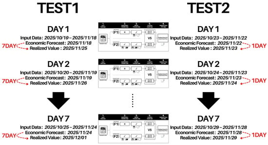
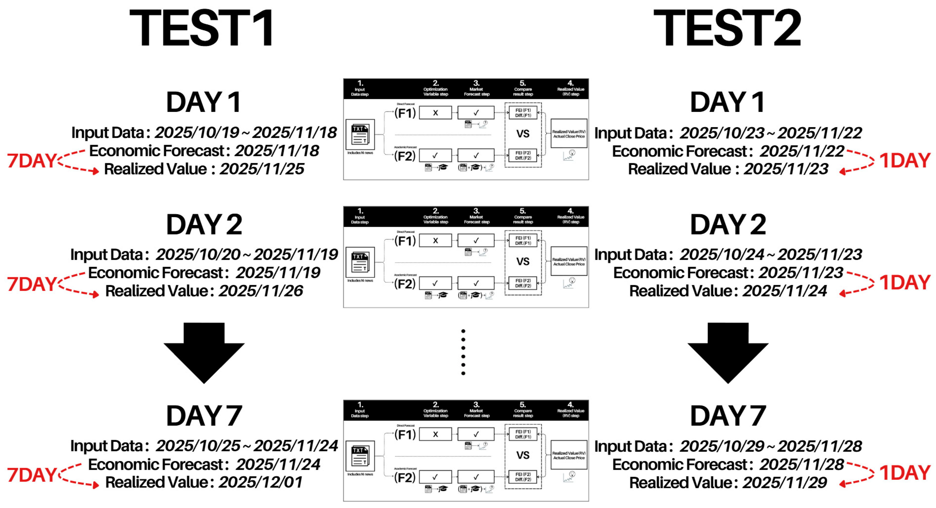
This study evaluates F1 and F2 across two forecast horizons (Test1 and Test2) to assess forecasting robustness (see Figure 3). Both tests use a 7-day Rolling Validation approach, differing in the time distance of the forecast horizon.
Figure 3.
Experimental Design of Forecast Horizons and Rolling Validation.
- Test1 (7-Day Forecast Horizon):Simulates medium-term wave forecasting. The model infers on baseline day (T) to forecast (T + 7) market values (e.g., 25 November 2025 from 18 November 2025). This tests whether F2 maintains long-term guidance effectiveness amid extended uncertainty.
- Test2 (1-Day Forecast Horizon):Simulates real-time reaction forecasting. The model infers on the baseline day (T) to forecast (T + 1) market values (e.g., 23 November 2025 from 22 November 2025). This evaluates LLM sensitivity to new market data and F2’s forecasting accuracy under ultra-short-term conditions.
- Rolling Validation Mechanism:A 7-day replication design dilutes date-specific errors, accumulating 28 forecast datasets for robust quantitative analysis.
- Identical Text Input Windows:Particularly, it is important to mention that T + 1 and T + 7 forecasts rely on identical text input windows. On any given experimental day T, whenever applicable, the same ‘Integrated Context’ (HIPES) is provided to both F1 and F2.
3.2. Research Instrument and Data Collection
This subsection outlines the data scope, including news sources, 75 IEIs, and their closing value (i.e., Realized Value, RV) methodology. Without loss of generality, data aggregation, transformation/optimization, prompt engineering, and LLM configuration are detailed as follows.
3.2.1. Data Aggregation (Rolling Window)
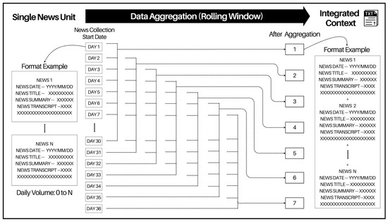
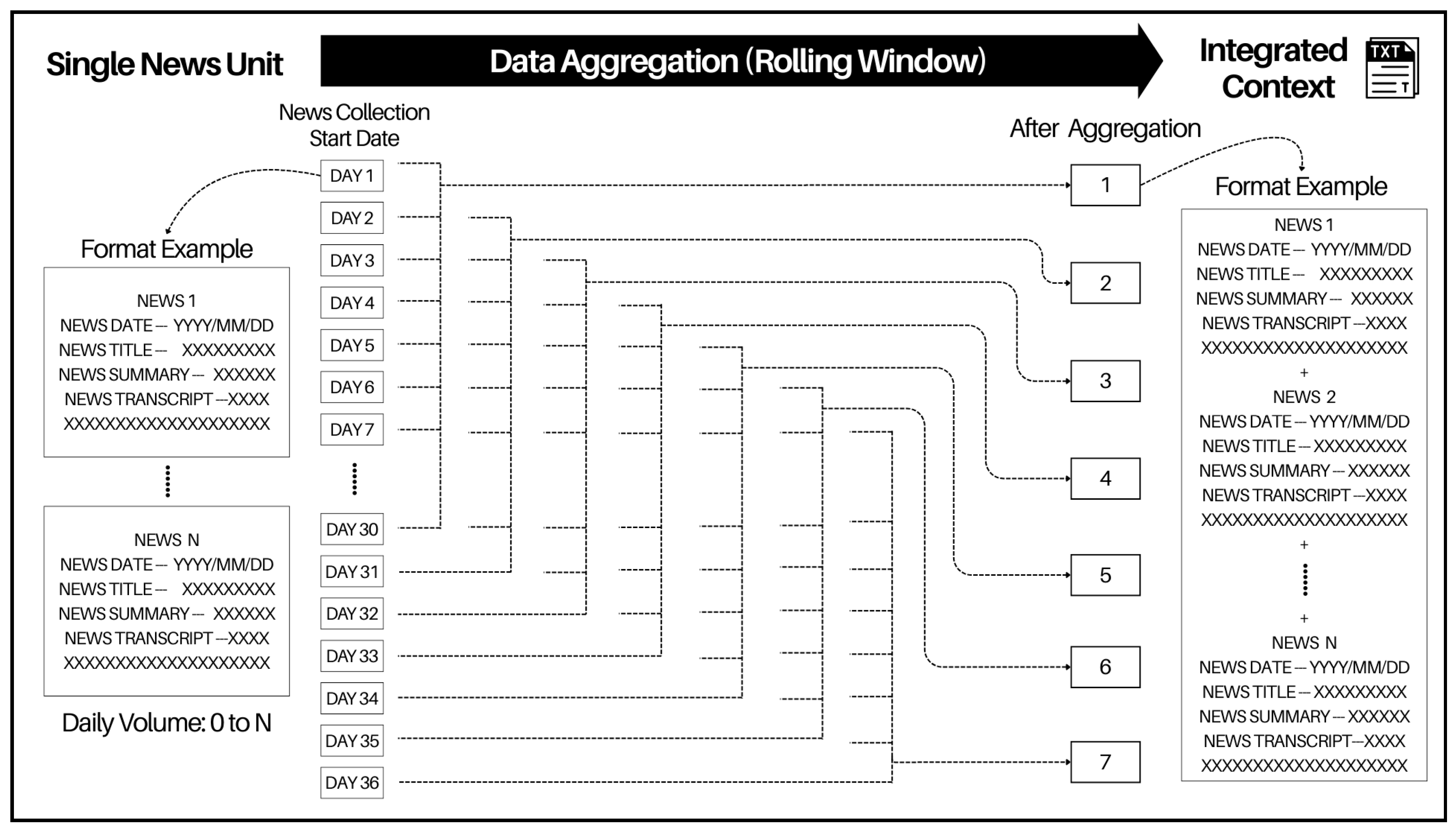
Figure 4 illustrates the process of converting “Single News Unit” text into “Integrated Context”.
Figure 4.
Data Aggregation (Rolling Window).
- Single News Unit:Core textual data are sourced from HIPES by international leaders, systematically extracted from Rev.com’s verbatim transcripts, and then standardized into .txt files containing (News Date), (News Title), and (News Transcripts), and these serve as foundational units for merging.
- Integrated Context:It aggregates 30 days of “Single News Unit” texts (T-30 to T-1) to capture cumulative semantic context, which is then merged into a single long-text file, forming the complete input basis for LLM inference.
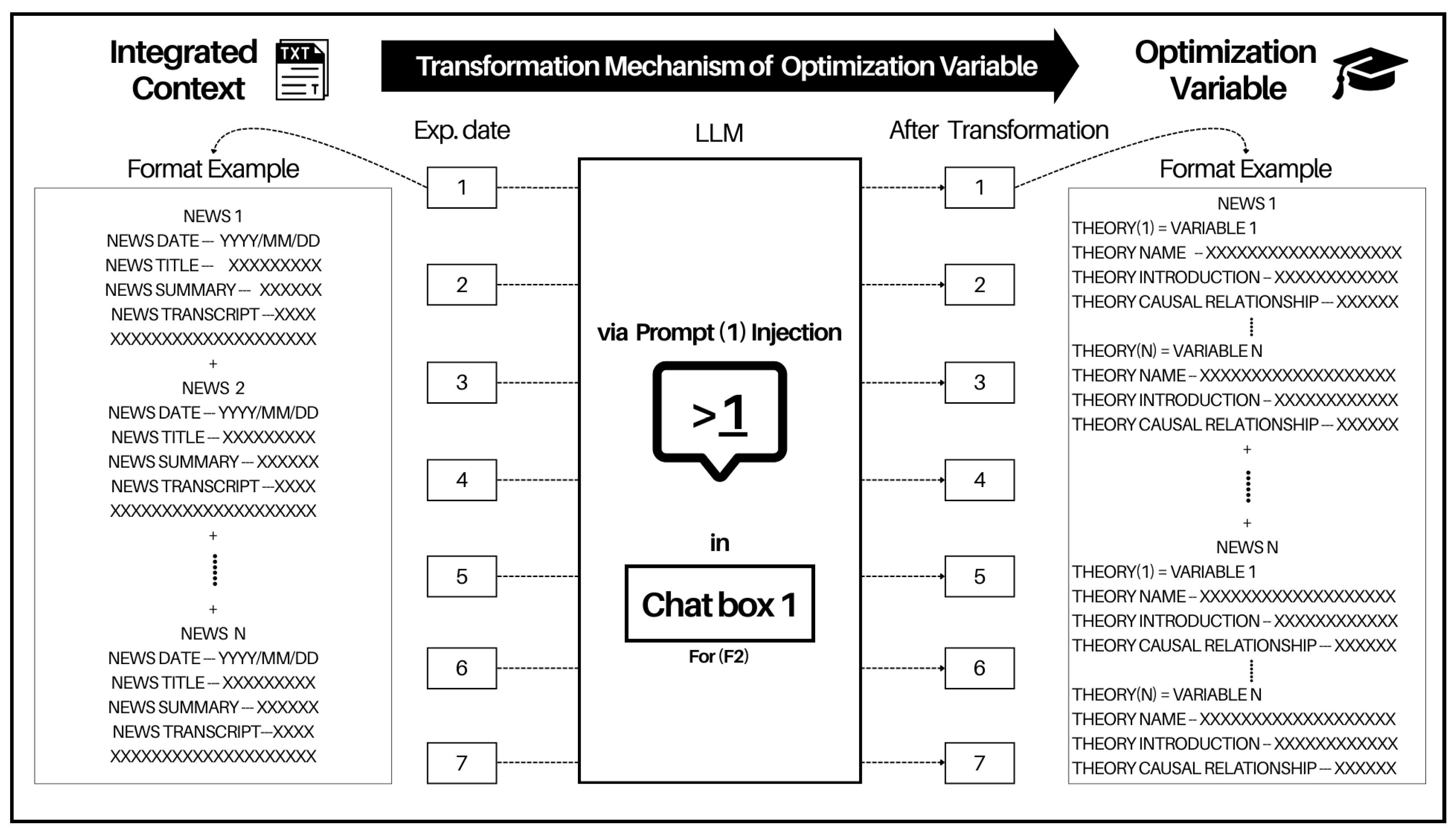
3.2.2. Transformation Mechanism of Optimization Variable
Figure 5 illustrates the mechanism for generating the Optimization Variable, and Appendix A presents a case study of this process. By converting Integrated Context into pure text, the study establishes the academic theory foundation for the Optimization Variable. An LLM serves as the semantic processing engine, using Prompt (1) Injection to automatically extract implicit Academic Theory from news content. This reshapes the extracted theory into a structured Optimization Variable, defining a standardized conversion process for applicable academic theories, their introductions, and key causal relationships.
Figure 5.
Transformation Mechanism of Optimization Variable.
3.2.3. Mechanism of Economic Forecast
Figure 6 illustrates the comparison of two input configurations. F1 uses only Integrated Context to simulate forecasts based solely on news content; F2 combines Integrated Context with the Optimization Variable from the prior stage to generate forecasts. Both configurations generate forecasts of closing prices for the 75 IEIs on a specific day.
Figure 6.
Mechanism of Economic Forecast.
3.2.4. LLM Model Configuration and Experimental Environment
This study uses Google Gemini (Ver. 3 Pro) as the core inference engine, leveraging its Long-Context Capability and abstract reasoning strengths to address text truncation challenges in traditional models. Integration with Google’s cloud services (e.g., Google Sheets, Cloud) can simplify database management.
3.3. Analysis Method
To evaluate the accuracy and robust differences between F1 and F2, this study employs a multidimensional validation framework. It includes the FEI metric for accuracy assessment, Diff. values for performance comparison, paired sample t-tests for credibility validation, and volatility analysis of the 75 IEIs, forming the basis for empirical analysis. Using FEI metrics and statistical tests, this study assesses F1 and F2’s forecasting accuracy for 75 IEIs. The integration of 1-day and 7-day macro perspectives enables a comprehensive evaluation of system stability and practical effectiveness over different time spans.
3.3.1. Mathematical Framework of Forecast Estimate Index (FEI)
The FEI quantifies forecasting accuracy through a standardized (Min-Max Ratio) algorithm, ensuring scores range between 0 and 1. A value closer to 1 indicates higher accuracy, while 0 signifies significant deviation. The formula calculates the smaller value as the numerator and the larger as the denominator, eliminating directional bias in overestimation or underestimation.
Definition 1
(Forecast Estimate Index (FEI)). Let P and RV represent the forecasted and realized closing prices/values of the 75 IEIs on a specific day; then FEI can be defined as
Score = 1: Perfect forecast accuracy ( = ).
Score ≈ 1: High accuracy ( close to ).
Score = 0: Low accuracy ( and differ significantly).
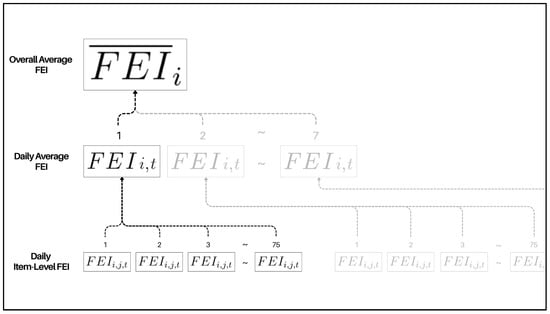
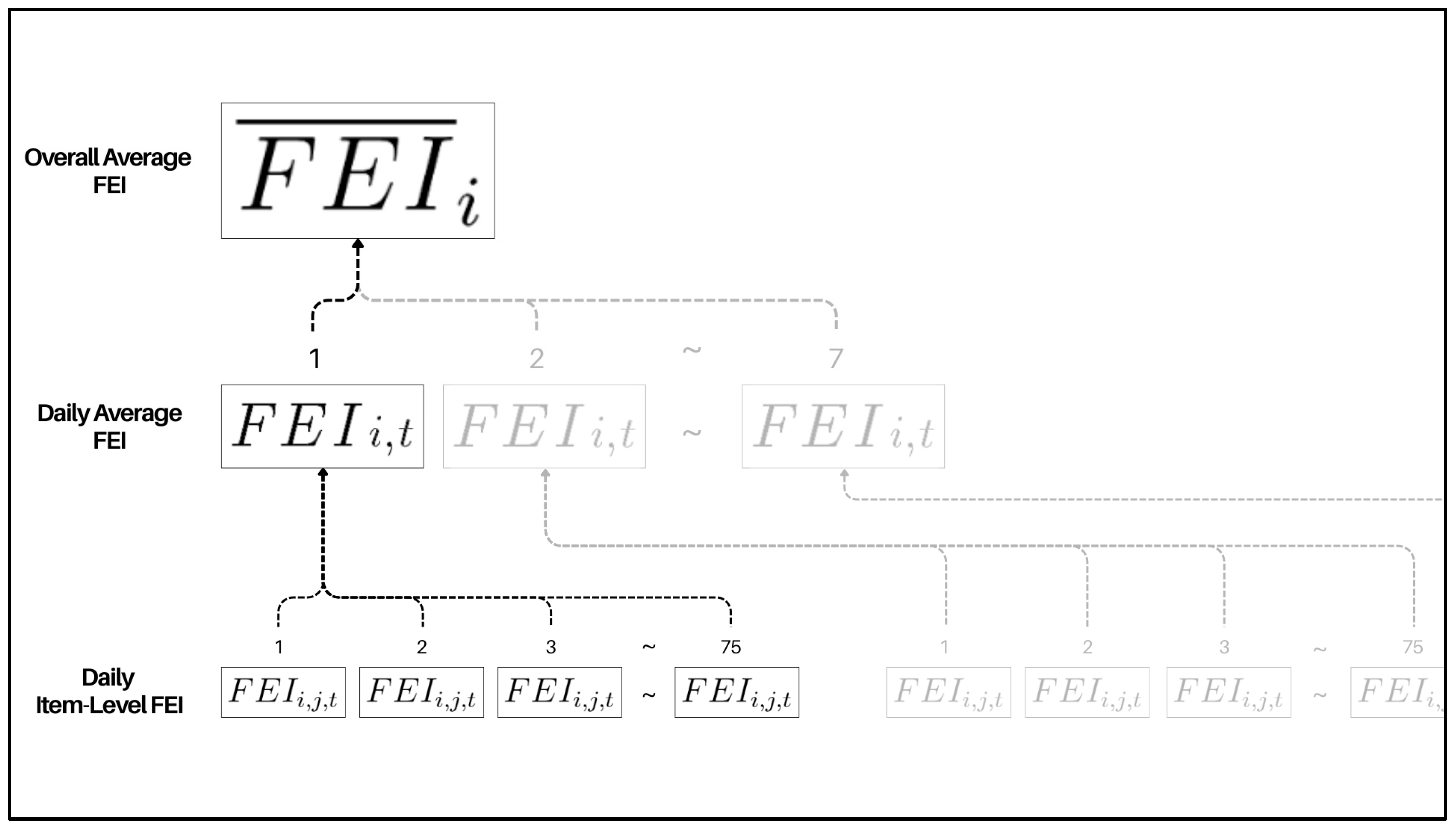
This study structures the FEI calculation (1) into three hierarchical levels for macro-level analysis: (Daily Item-Level FEI, ), (Daily Average FEI, ), and (Overall Average FEI, ). Figure 7 illustrates their relationships.
Figure 7.
Mathematical Framework of Forecast Estimate Index (FEI).
= (Model Index): 1 = Direct Forecast (F1), 2 = Academic Forecast (F2).
= (Asset Index): Items 1–75 of the 75 IEIs.
= (Time Index): One day within the 1st–7th days of the experiment.
- Daily Item-Level FEI ()
Definition 2
(Daily Item-Level FEI (). We define this metric to calculate the daily forecast accuracy of the 75 IEIs for a specific date t, such as gold or crude oil, reflecting individual asset performance.
- 2.
- Daily Average FEI ()
Definition 3
(Daily Average FEI (). It aggregates the “Daily Item-Level FEI” values of all 75 indicators on a given day, providing a macro-level assessment of forecast accuracy across five global asset categories (e.g., Commodities, Indices, Exchange Rates, Crypto, and 10Y Yield).
- 3.
- Overall Average FEI ()
Definition 4
(Overall Average FEI (). This metric averages the “Daily Average FEI” over 7 consecutive days, representing the experiment’s long-term stability and overall accuracy. It serves as the core metric to validate whether F2 significantly outperforms F1 in the full experimental period (e.g., Test1 or Test2’s 7-day rolling window).
3.3.2. Item-Level Difference Framework (Diff.)
- Framework Design
Definition 5
(Item-Level Difference (Diff.)). To assess the performance gap between F1 and F2 across the 75 IEIs, the “Daily Item-Level FEI” values over seven days are averaged. The difference (Diff.) is calculated as F1–F2, with 0 as the baseline. A larger absolute Diff. value indicates stronger forecasting performance. Positive Diff. values for F1 and negative Diff. values for F2 signify superior performance for F1 and F2, respectively.
Diff. > 0: F1 outperforms F2; the farther from 0, the greater the advantage.
Diff. = 0: Equal performance; no clear superiority.
Diff. < 0: F2 outperforms F1; the farther from 0, the greater the advantage.
- 2.
- Quartile Analysis for Strength Distribution
Definition 6
(Quartile Analysis). To validate robustness, the experiment employs a multidimensional hierarchical mechanism. The absolute Diff. values are categorized into four strength intervals (0%, 25%, 50%, 75%) using quartile thresholds. This distribution visually quantifies the forecasting performance of F1 and F2 across all 75 indicators, emphasizing the magnitude of their advantages in forecasting.
3.3.3. Paired Sample t-Test
SPSS 20.0 is used to validate statistical robustness through paired sample correlation coefficients, which assess model synchronization. Significantly high correlation confirms consistent market response and rational paired comparison. A paired sample t-test further evaluates statistical results (e.g., p-values). Significant outcomes (p < 0.05) indicate systematic performance differences between models (F1 and F2), excluding random fluctuations.
3.3.4. Market Characteristics and Volatility Stratification
Asset Volatility is introduced as a key metric to quantify “Forecast Difficulty.” Daily return standard deviations for the 75 IEIs are calculated and averaged. And then apply (6) Quartile Analysis, which divides the result into four volatility tiers (0%, 25%, 50%, 75%) to highlight performance disparities. This stratification can clarify whether F2 demonstrates greater potential in managing high-volatility assets than in low-volatility environments.
Definition 7
(7-day volatility, ). To assess forecast difficulty, 7-day volatility is computed for each asset i as the standard deviation of daily returns over a one-week period.
: 7-day volatility of asset .
: daily return of asset on day .
: average daily return of asset over the 7-day period.
4. Empirical Results and Analysis
4.1. Sample Description and Research Rigor
4.1.1. Experimental Design and Time Series Structure
This study outlines the data framework for “Integrated Context” and “Optimization Variable,” with Table 3 detailing the experimental timeline, data collection periods, forecast execution dates, and verification closing dates (i.e., RV Date). The table quantifies daily News Count and Academic Theory Count, establishing a transparent, replicable experimental benchmark.
Table 3.
Experimental Schedule Table and Contents.
The study evaluates F1 and F2 through two scenarios:
- Test1 (T + 7): Long-Term Trend Forecasting:Uses “Integrated Context” for both models, with “Optimization Variable” exclusive to F2. Forecasts are executed on the experiment day, with final metrics derived from the RV Date closing price over a 7-day horizon.
- Test2 (T + 1): Short-Term Immediate Forecasting:Focuses on ultra-short-term price fluctuations using a rolling window strategy. Forecasts are based on a 1-day horizon, with RV Date closing prices used for analysis.
4.1.2. Data Input to Experiment
The data inputs for each experimental day are described as follows.
- News Count:Daily input for F1 and F2 includes 18–23 HIPES.
- Academic Theory Count:F2 incorporates 38–56 academic theory features extracted by LLMs, representing causal logic and economic patterns from transcripts.
4.1.3. Sources and Rules for Final Value Acquisition
- Benchmark Indicators:75 IEIs (uniformly distributed across five asset categories) sourced from Trading Economics (tradingeconomics.com).
- Closing Price Rules:Daily closing prices are used as the baseline. Non-trading days (weekends and holidays) apply a carry-forward rule, retaining the previous valid trading day’s closing price to preserve the time series’ integrity.
4.2. Measurement Result Analysis
This subsection systematically evaluates F2’s superior performance over F1 in forecasting accuracy and stability through multidimensional quantitative analysis of overall metrics, asset distribution, and performance gaps.
4.2.1. Daily Average and Overall Average FEI Comparison
As shown in Table 4, F2 demonstrates consistent accuracy advantages (in terms of Daily Average FEI and Overall Average FEI) over F1 across all experimental scenarios in Test1 (T + 7) and Test2 (T + 1).
Table 4.
Comparison of Daily Average and Overall Average FEI Across F1 and F2.
- Comprehensive Superiority:In (Panel A), F2 achieves higher daily average FEI values than F1 on all days (Day 1–Day 7). In (Panel B), F2’s overall average FEI reaches 0.803 in Test1 (vs. 0.777 for F1) and 0.796 in Test2 (vs. 0.777 for F1), highlighting the Optimization Variable’s role in enhancing market dynamics capture. For the 75 IEIs, F2’s FEI values align more closely with actual observations.
- Stability and Robustness:Across time domains, F2 maintains FEI above 0.783 at all-time points, peaking at 0.811 on Day 4 in Test1. Its consistent performance under Test1 and Test2 settings confirms the Optimization Variable’s robustness in enhancing forecasting accuracy across various time windows.
- Forecasting Accuracy Metric (FEI vs. MAE/MSE):In evaluating MAE/MSE (which are popular forecasting accuracy metrics), all errors contribute to MAE/MSE unequally. While the larger errors contribute more to MAE than smaller errors, those larger errors contribute even more to MSE than smaller ones. Although FEI calculations mitigate the uneven contributions suffered by MAE/MSE, we still calculate MAE and MSE based on the data used in Table 4 and derive Table 5 and Table 6 for comparison purposes, and the results (in Table 4, Table 5 and Table 6) are consistent, showing F2 outperforms F1 in overall forecast performance.Table 5. Comparison of Daily Average and Overall Average MAE Across F1 and F2.Table 6. Comparison of Daily Average and Overall Average MSE Across F1 and F2.
- Additional Weekly Replications on Overall Average FEI Validation:This study is anchored in the core empirical evidence presented in Table 4 (Week 1), supplemented by three additional weekly validations to ensure robustness and mitigate the influence of temporal randomness. The results demonstrate that the F2 framework maintains a persistent and stable performance advantage against F1 in terms of Overall Average FEI across all observation periods, with further details described as follows:
Test 1 (T + 7):
The superiority of F2’s Overall Average FEI is consistently observed from 4 weekly experiments: Week 1 (F2’s 0.803 > F1’s 0.777), Week 2 (F2’s 0.801 > F1’s 0.776), Week 3 (F2’s 0.797 > F1’s 0.772), and Week 4 (F2’s 0.794 > F1’s 0.771).
Test 2 (T + 1):
F2 likewise maintains its lead throughout the validation: Week 1 (F2’s 0.796 > F1’s 0.777), Week 2 (F2’s 0.792 > F1’s 0.776), Week 3 (F2’s 0.787 > F1’s 0.775), and Week 4 (F2’s 0.782 > F1’s 0.773).
These weekly experimental results provide robust evidence suggesting that the F2 framework possesses significant and persistent predictive superiority as well as systematic robustness.
4.2.2. Daily Item-Level Win Statistics by Asset Category and FEI Intensity (7-Day Mean)
Table 7 evaluates the seven-day average FEI values of the 75 IEIs, defining higher FEI as “wins” and analyzing performance across five asset categories. The analysis first examines overall win frequency (Panel A) and then explores FEI intensity distributions (Panels B–E).
Table 7.
Daily Item-Level Win Frequency Statistics by Asset Category and FEI Intensity.
- Overall Win Frequency (Panel A):In Test1 (T + 7), F2 achieved 40 wins, significantly outperforming F1’s 34. In Test2 (T + 1), F2’s lead expanded to 43 wins, while F1 secured only 31. This underscores F2’s consistent superiority across asset categories, particularly in Crypto and Exchange Rates, where it dominates. F1 retains strengths in Commodities and Indices, while F2 shows marginal advantages in 10Y Yield.
- High Accuracy Range (Panel B):While total wins are closely contested (Test1: 29 vs. 28; Test2: 27 vs. 29), F2’s wins cluster heavily in Exchange Rates and Crypto. This highlights the effectiveness of Academic Theory integration via the Optimization Variable, enabling F2 to outperform F1 in high-accuracy scenarios.
- Mid-to-High Accuracy Range (Panel C):F2 maintains dominance in Crypto and Exchange Rates, securing 6–3 wins in Test2 (T + 1) compared to a 5–5 tie in Test1 (T + 7). This reinforces its targeted accuracy in challenging financial assets, Crypto and Exchange Rates.
- Mid-to-Low and Low Accuracy Ranges (Panels D, E):F1 struggles with near-zero wins, while F2 records 6–7 wins (Panel D) and 1–1 wins (Panel E). This demonstrates F2’s resilience in extreme forecasting conditions, compensating for F1’s limitations.
- Summary:Table 7 reveals F2’s structural advantages in operational resilience and domain-specific accuracy. By integrating Academic Theory through the Optimization Variable, F2 achieves focused superiority in various asset categories, solidifying stability across all intervals and setting the foundation for further analysis of performance improvements (see Table 8).Table 8. Daily Item-Level Performance Differentials (Diff.) by Asset Category and FEI Intensity.
4.2.3. Forecast Performance Differential Analysis
Building on prior discussions of win frequency, Table 8 extends the analysis to quantify forecast performance differences. Daily Item-Level FEI values are calculated as seven-day arithmetic means, with differences (Diff. = F1 − F2) defining performance gaps. Quartile Analysis divides these gaps into four intensity intervals (Panels A–D), reflecting varying degrees of model superiority. Panel A (Top 75–100%) highlights F2’s strongest performance gains, while Panel D (Bottom 0–25%) indicates minimal gaps.
- High-Intensity Interval (Panel A):In the top 25% of samples with the largest gaps, F2 dominates: Test1 (T + 7) yields 15 wins (vs. F1’s 5), and Test2 (T + 1) records 14 wins (vs. F1’s 5). Crypto shows 12/15 wins in both tests, underscoring F2’s ability to correct extreme volatility, where F1 struggles.
- Moderate-Intensity Interval (Panel B):As gaps narrow, F1’s competitiveness rises. F2 maintains a slight lead (10 vs. 9 wins in Test1 and Test2), but F1 closes the gap to 9–8 wins. F1 excels in traditional assets like Commodities (4:2 win ratio in Test1) and Exchange Rates, while F2 retains advantages in 10Y Yield.
- Moderate-Low-Intensity and Low-Intensity Intervals (Panels C, D):F1’s dominance grows further, achieving 12:10 wins in Test1 (Panel C). This reflects F2’s core strength in high-volatility assets, where it delivers significant corrections, contrasting with F1’s limited adaptability in extreme conditions.
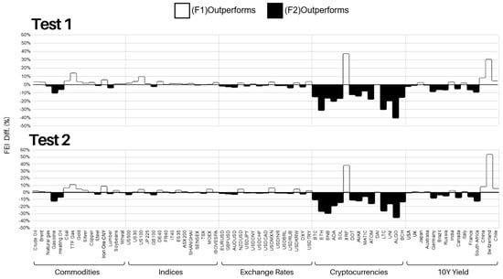
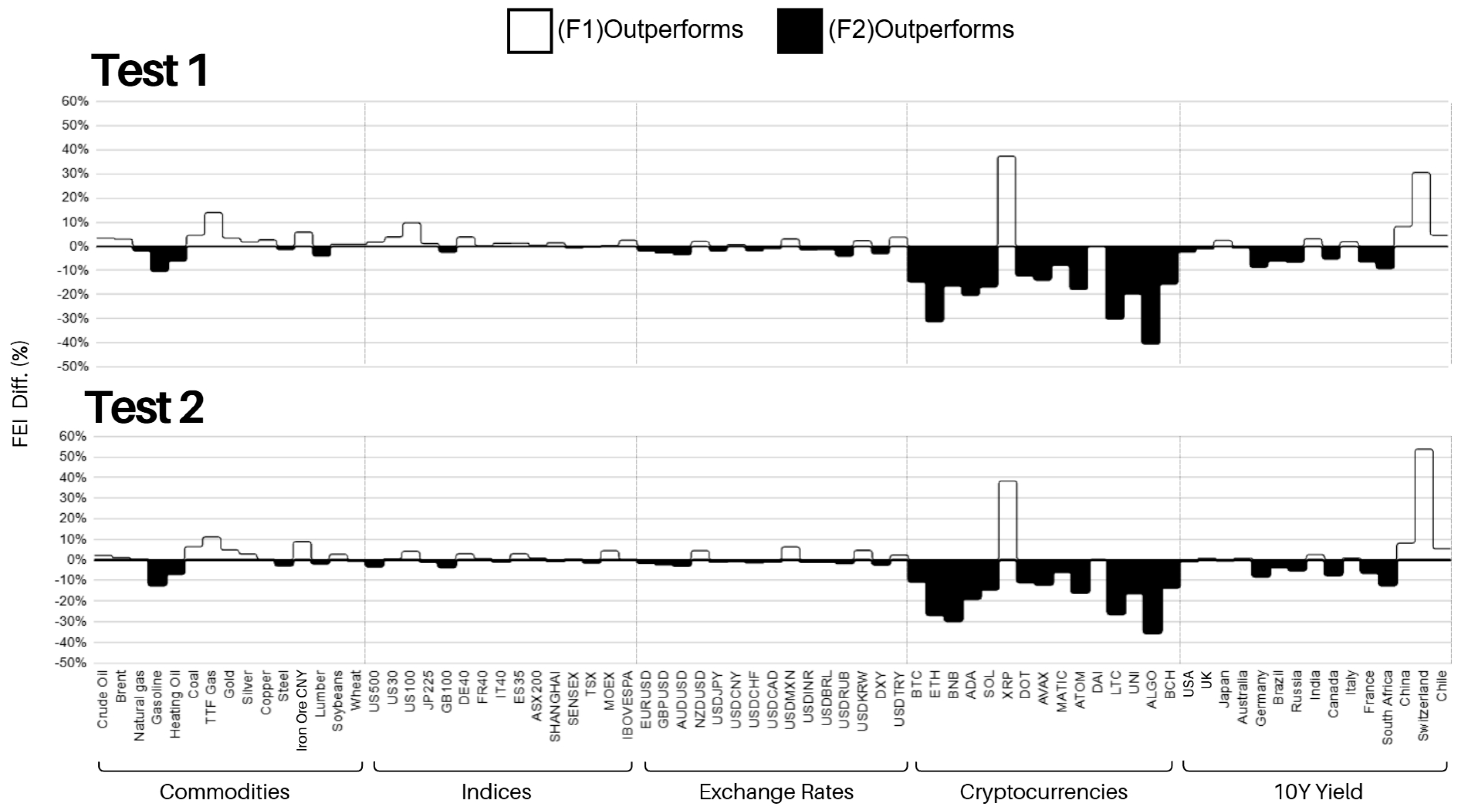
Table 8 confirms that F2 leads in overall win rate and demonstrates significant forecast performance improvements in high-volatile scenarios (Panel A), particularly in cryptocurrency markets. Figure 8 visualizes the Performance Differential between F1 and F2 across five asset categories, with the zero-axis separating their advantages: Hollow bars indicate F1’s superiority, while Solid Black bars highlight F2’s dominance.
Figure 8.
Daily Item-Level Performance Differentials (Diff.) by Asset Category and FEI Intensity (7-Day Mean).
Key Observations:
- Systematic Dominance in Cryptocurrencies:F2 exhibits consistent superiority in cryptocurrencies, with negative values ranging from −20% to −40% (except for XRP). This underscores its theoretical advantage in high-volatile assets, surpassing F1’s marginal gains.
- Competitive Parity in Traditional Assets:In commodities, indices, and exchange rates, F2 and F1 show close competition (±10% fluctuations). F1 retains a slight edge in mature markets like US100 and DE40, supporting the relevance of the random walk hypothesis in efficient markets.
- Robustness across Tests:Test1 and Test2 produce highly consistent patterns, with F2’s deep black valleys in cryptocurrencies and F1’s minor oscillations in commodities aligning across both tests. This validates the findings as generalizable, not data-specific.
- Summary:F2’s integration of Academic Theory via the Optimization Variable drives its structural edge in high-impact scenarios, while F1 gains traction in moderate conditions. These results align with Table 7, reinforcing the efficacy of F2’s integrated framework.
4.3. Structural Model Analysis and Hypothesis Testing
This subsection validates the experiment’s credibility through rigorous statistical testing. Two stages are employed: First, we analyze four sets of Daily Item-Level FEI data from Test1 (F1, F2) and Test2 (F1, F2) using SPSS. Paired Sample t-tests assess model correlations and forecast differences’ statistical significance, excluding random error and confirming robust results. Second, this study quantifies asset price volatility of 75 IEIs to demonstrate F2’s adaptability across various closing price environments.
4.3.1. Paired Samples Correlations
Table 9 presents paired sample correlation coefficients between F1 and F2 in Test1 (T + 7) and Test2 (T + 1). Results show high positive correlations (r = 0.839~0.938) across all forecast periods (Day 1–7), with ( < 0.001) for all outcomes. This confirms F2 aligns with F1 in capturing market trends while improving Accuracy without altering the foundational forecasting structure.
Table 9.
Paired Samples Correlations between F1 and F2 Models.
4.3.2. Mean Value, Standard Deviation, and Paired Samples t-Test
Table 10 evaluates the statistical significance of forecast performance differences between F1 and F2 by evaluating their mean values and standard deviations and conducting a paired sample t-test between them.
Table 10.
Paired Sample t-test Results of Forecast Estimate Index (FEI) for F1 and F2 Models.
- Mean Value, Standard Deviation, and Stability:Across all forecast days in Test1 and Test2, F2’s FEI Mean consistently exceeds F1’s, while F2’s FEI SD is significantly lower, indicating superior accuracy and stability.
- Statistical Significance:t-test results confirm significant performance differences (p < 0.05) at multiple forecast points. In Test1, significant differences occur on Day 1 (p = 0.050 *), Day 3 (p = 0.038 *), and Day 4 (p = 0.029 *). Test2, Day 1 (p = 0.049 *), also shows significance. Negative values (F1–F2) further validate F2’s higher FEI, affirming the substantive contribution of the Academic Forecast (F2) approach to improved forecast accuracy.
Table 9 and Table 10 provide further empirical evidence: Table 9 presents the results of paired-sample t-tests, confirming statistical significance in the performance difference. Meanwhile, Table 10 illustrates the mean values, intuitively demonstrating that F2 consistently outperforms F1 throughout the entire 7-day period.
4.3.3. Distribution of Closing Price Volatility Intensity
Table 11 employs quartile analysis to categorize assets based on volatility intensity (i.e., STDEV.S) derived from 75 IEIs. Assets are divided into four volatility zones: Top 75–100% (highest volatility), Second (50~75%), Third (25~50%), and Bottom 0–25% (lowest volatility), highlighting F2’s adaptability across diverse market environments.
Table 11.
Distribution of Closing Price Volatility Intensity across Asset Categories.
- High-Volatility Concentration:Cryptocurrencies dominate the Top Quartile (STDEV.S ≥ 1.55%), accounting for 14/15 assets, establishing them as a “high-risk, high-nonlinearity” market representative.
- Medium-to-Low Volatility (the Second, Third, and Bottom Quartiles) Distribution:10Y Yield (8/15) occupies the Second Quartile (1.55–0.74%), Indices (9/15) the Third Quartile (0.74–0.41%), and Exchange Rates (11/15) the Bottom Quartile (0.41–0%).
- Environmental-Performance Alignment:Overall, our analysis results align with prior analyses (Table 7 and Table 8; Figure 8). Table 11 confirms Crypto’s high volatility (≥1.55%), matching F2’s exceptional performance: 13/15 wins in Table 7 (Panel A) and 8.14% Forecast Performance improvement in Table 8 (Panel A). Figure 8 further validates this trend. These findings affirm that F2’s Academic Forecast-oriented Optimization Variables outperform F1 in volatile markets, demonstrating both practical efficacy and academic significance.
5. Conclusions
This study aims to investigate the effectiveness of Academic Forecast (F2) in utilizing the Optimization Variable to guide LLM for forecasting IEIs based on HIPES. Through empirical analysis of the 75 IEIs and paired sample t-tests using SPSS, it was confirmed that the Optimization Variable significantly and positively influences Forecast Accuracy (in terms of Daily Item-Level FEI, Daily Average FEI, and Overall Average FEI) and Forecast Advantage Breadth (75 IEIs). The study results verify that, compared to F1, the Academic Theory-guided F2 is more effective in increasing overall Forecast Accuracy and demonstrates dominant performance in specific, high-volatility asset categories.
The results demonstrate that F2 significantly outperforms F1 in overall forecast performance. Regardless of whether in Test1 (T + 7) or Test2 (T + 1), the Overall Average FEI and Daily Average FEI of F2 exhibit significantly better accuracy (values closer to 1). By leveraging the causal logic of Academic Theory as an Optimization Variable, the model can more effectively capture market reactions, making the forecast values closer to actual trends. F2’s overall average FEI reaches 0.803 in Test1 and 0.796 in Test2, compared to 0.777 for F1 in both cases (shown in Table 4). These results indicate that F2 outperforms F1 in overall accuracy, achieving a +2.25% gain. This confirms RQ1: Compared to F1, which generates indicators directly, F2, which incorporates Academic Theory as an Optimization Variable, significantly improves the accuracy and stability of forecasting overall IEIs.
Experiment results indicate that F1 and F2 differ significantly in forecast accuracy across asset categories. When performance differentials exceed 8.14%, F2 captures markedly more items (14.5 vs. 5), with particularly strong forecasting performance in high-volatile assets such as cryptocurrencies, as documented in Table 7 and Table 8 and Figure 8. It not only shows significant improvements in the frequency of Forecast Value Proximity and the intensity of Forecast Performance Gains. In contrast, F1 demonstrates stable explanatory power in forecasting fundamental assets like Commodities and Indices, with notable advantages in the frequency of accurate forecasts. This aligns with the Adaptive Market Hypothesis [40], which emphasizes the dynamic evolution of market efficiency. This may be because Cryptocurrency markets are highly susceptible to political sentiment and speculative psychology, and the Optimization Variable of F2 successfully captures such non-linear volatility. Conversely, Commodities and Indices are more influenced by physical supply-demand dynamics, making F1’s intuitive Forecast more efficient due to lower noise levels. This confirms RQ2: Based on experiment results, different types of asset categories (e.g., Commodities Market, Stock Market Indices, Foreign Exchange Rates, Cryptocurrencies, 10-Year Government Bond Yield) exhibit distinct and significant forecast advantages for both F1 and F2.
The distinct differences in forecast advantages between F1 and F2 demonstrate that the optimal forecast strategy for the 75 IEIs cannot be monopolized by either model alone. The two models form a complementary structure: F1 is suitable for Stable Assets (e.g., Commodities and Indices), while F2 excels in High-Volatility Assets (e.g., Cryptocurrencies). Although F2 achieves overall statistical significance, the stability of F1 remains noteworthy. This finding strongly underscores the limitations of single-model approaches and provides essential empirical evidence for developing an Optimized Portfolio Strategy in the future.
6. Implications
6.1. Managerial Implications
Beyond traditional machine learning reliance on historical price data, this study confirms that integrating unstructured information (e.g., real-time political and economic sentiment, news text) into analysis can enhance forecast accuracy. By transforming such readily available environmental data into economic forecasting inputs and innovating through the introduction of Optimization Variables into LLM, organizations can improve forecast performance. This insight urges managers to actively utilize unstructured data as a new pathway to discover “more superior forecasting methods,” rather than being confined to existing forecast frameworks.
Given the empirical evidence of domain complementarity in forecasting models, forecasters should adopt a Customized Forecast Portfolio strategy. For example, Stable Assets (e.g., Commodities and Indices) are suitable for F1, while High-Volatility Assets (e.g., Cryptocurrencies) are better suited for F2. Other assets, like Exchange Rates and 10Y Yield can leverage the complementary structure of F1 and F2. This combination strategy may more or less enhance overall forecast performance.
This study presents a high-return, low-barrier-to-entry implementation model, F2, which has the key ability to capture extreme market situations for providing timely advice/opinions/countermeasures but with low deployment costs. It requires only generic LLM tools (e.g., Gemini) combined with basic data management (e.g., Google Sheets). This implies that forecasters can deploy this forecast system with high effectiveness, without significant computational resources or development costs.
This research shows that incorporating ATBOV into LLMs can equip governments, enterprises, and individual investors with an AI application research tool for economic forecasting, enabling them to quickly make high-quality decisions that go beyond market intuition in response to sudden, high-impact political and economic events.
6.2. Academic Implications
Previous studies have rarely addressed how to refine LLMs’ economic reasoning. This study confirms that combining Integrated Context—which includes transcripts of HIPES—with the ATBOV can effectively imbue LLMs with causal logic, significantly improving the forecast accuracy across five asset categories covering 75 IEIs. Indeed, this study provides empirical support for LLM-based forecast optimization.
For the most challenging task of forecasting the market trend of high-volatility assets—Cryptocurrencies—this study demonstrates that ATBOV plays a decisive role in correcting model biases. This validates the unique academic value of the theoretical frameworks in filtering high-volatility noise and fills a theoretical gap in the literature regarding how LLMs equipped with ATBOV can cope with extreme market volatility.
7. Limitation and Future Work
This study currently focuses on the 75 IEIs from tradingeconomics.com, using their closing prices as the realized value (RV), with a sample evenly distributed across five major asset categories. To enhance the model’s applicability, future research may remove this sample constraint and allow users to replace and expand the forecasted targets (in addition to the 75 IEIs) based on specific needs. This can not only validate the model’s flexibility but also explore its forecasting performance across different sectors of IEIs.
This study currently focuses on U.S. political and economic statements within a specific period, with relatively limited information sources. Future research could expand this experimental framework by incorporating Integrated Context with heterogeneity and real-time characteristics. In addition to expanding the data scope to include multi-country political and economic statements, corporate earnings reports, social sentiment, and radical news, researchers may also test adjustments to data collection frequency, forecast horizons (T + n), and experiment time granularity to evaluate whether different temporal windows yield any potential forecast performance improvements.
Given the accuracy and performance improvements achieved by ATBOV, future studies may explore multimodal and behavioral causality-oriented Optimization Variables. Incorporating elements such as voice tone, micro-expression recognition, and behavioral finance factors in follow-up research could further transform or advance non-textual market sentiment into structured data or knowledge, thereby enhancing LLMs’ ability to explain and/or cope with irrational market fluctuations.
Due to experimental resource limitations, this study only validated results in the Gemini model environment. Future research may conduct replication studies on platforms with different LLM architectures, such as GPT-5, Grok, Claude, and so on. Cross-model validation may not only confirm the generalizability of the “theoretical optimization framework” but also allow for in-depth exploration of potential advantages of specific LLM models for desirable and applicable financial asset categories.
Author Contributions
Conceptualization, S.E.C. and K.-C.C.; Methodology, S.E.C. and K.-C.C.; Software, K.-C.C.; Validation, S.E.C. and K.-C.C.; Formal analysis, S.E.C. and K.-C.C.; Investigation, S.E.C. and K.-C.C.; Resources, S.E.C. and K.-C.C.; Data curation, S.E.C. and K.-C.C.; Writing—original draft, S.E.C. and K.-C.C.; Writing—review and editing, S.E.C. and K.-C.C.; Visualization, K.-C.C.; Supervision, S.E.C.; Project administration, S.E.C.; Funding acquisition, S.E.C. and K.-C.C. All authors have read and agreed to the published version of the manuscript.
Funding
This work was supported in part by the National Chung Hsing University, Taiwan.
Institutional Review Board Statement
Not applicable.
Data Availability Statement
The original contributions presented in this study are included in the article. Further inquiries can be directed to the corresponding authors.
Conflicts of Interest
The authors declare no conflicts of interest.
Appendix A
This Appendix A aims to supplement Figure 5 and Table 3 in the main text by providing a practical case study of mapping ‘Integrated Context’ to ‘Optimization Variable’. First, Figure A1 specifically demonstrates the empirical transformation process under the conceptual framework of Figure 5. Next, Table A1 summarizes and presents the key textual information of the ‘Integrated Context.’ Finally, Table A2 details the complete derivation process and output results of formally transforming this context into an ‘Optimization Variable’.
Figure A1.
e.g., demonstrating the Transformation Mechanism of Optimization Variable.
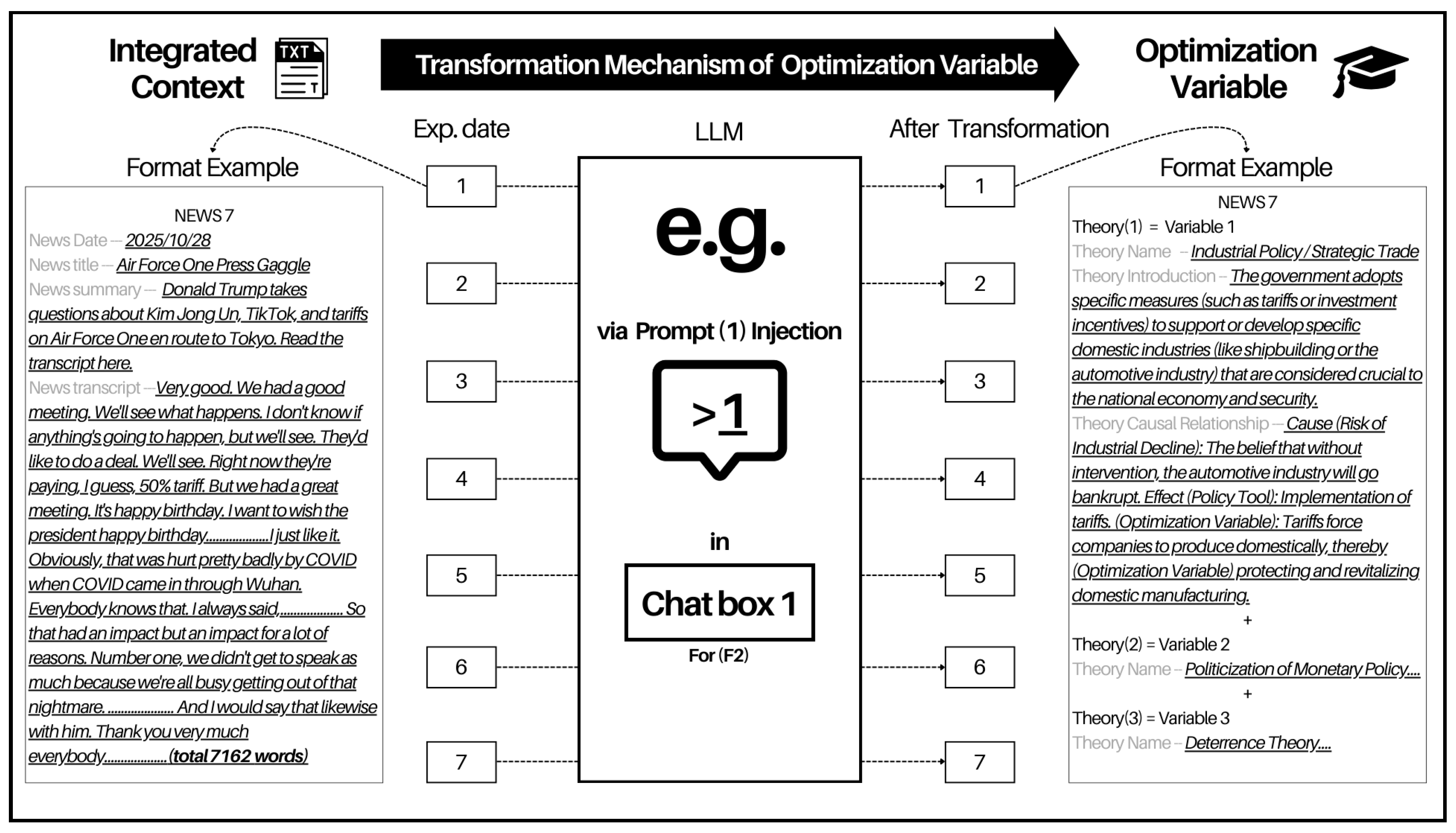
Table A1.
Take News 7 from the Day1 “Integrated Context” as an example.
Table A1 summarizes the key information of the ‘Integrated Context’ presented in Figure A1. The specific fields include: News Number, News Date, News Title, News Summary, and the complete News transcripts. This original data is recorded in plain text (.txt) format, with a total word count of 7162 words.
Table A2.
Take News 7 from the Day 1 ‘Integrated Context’ as an example to demonstrate the transformation into an Optimization Variable.
Table A2 summarizes the key information of the ‘Optimization Variable’ presented in Figure A1. Its specific fields encompass the Theory Name, Theory Introduction, and Theory Causal Relationship. As illustrated in Panels A through C of the table, the Large Language Model (LLM) successfully extracted three distinct academic theories from the raw text in Table A1. Each ‘Optimization Variable’ is constructed by aggregating multiple HIPES collected over a 30-day look-back period (T-30). From a single piece of HIPES, a diverse set of academic theories can be extracted. The transformation process is structured as follows: Panel A illustrates the derivation of Variable 1 from Theory (1), while Panels B and C demonstrate the respective mapping of Theory (2) to Variable 2 and Theory (3) to Variable 3. The structural combination of this information constitutes the ‘Optimization Variable’ as defined in this study. The core objective of this design is to operationalize the transformation mechanism of (Speech → Theory → Optimization Variable). By employing a rigorous academic framework to converge the originally divergent, unstructured corpora, this approach facilitates subsequent quantitative predictions and effectively reduces noise and divergence during model analysis.
References
- Caldara, D.; Iacoviello, M. Measuring Geopolitical Risk. Am. Econ. Rev. 2022, 112, 1194–1225. [Google Scholar] [CrossRef] [Scilit]
- Fu, K.; Zhang, Y. Incorporating Multi-Source Market Sentiment and Price Data for Stock Price Prediction. Mathematics 2024, 12, 1572. [Google Scholar] [CrossRef] [Scilit]
- Karpatne, A.; Atluri, G.; Faghmous, J.H.; Steinbach, M.; Banerjee, A.; Ganguly, A.; Shekhar, S.; Samatova, N.; Kumar, V. Theory-Guided Data Science: A New Paradigm for Scientific Discovery from Data. IEEE Trans. Knowl. Data Eng. 2017, 29, 2318–2331. [Google Scholar] [CrossRef] [Scilit]
- Shiller, R.J. Narrative Economics. Am. Econ. Rev. 2017, 107, 967–1004. [Google Scholar] [CrossRef] [Scilit]
- Baker, S.R.; Bloom, N.; Davis, S.J. Measuring economic policy uncertainty. Q. J. Econ. 2016, 131, 1593–1636. [Google Scholar] [CrossRef] [Scilit]
- Blinder, A.S.; Ehrmann, M.; Fratzscher, M.; de Haan, J.; Jansen, D.-J. Central Bank Communication and Monetary Policy: A Survey of Theory and Evidence. J. Econ. Lit. 2008, 46, 910–945. [Google Scholar] [CrossRef] [Scilit]
- Bianchi, F.; Gómez-Cram, R.; Kind, T.; Kung, H. Threats to central bank independence: High-frequency identification with twitter. J. Monet. Econ. 2023, 135, 37–54. [Google Scholar] [CrossRef] [Scilit]
- Hassan, T.A.; Schreger, J.; Schwedeler, M.; Tahoun, A. Sources and Transmission of Country Risk. Rev. Econ. Stud. 2024, 91, 2307–2346. [Google Scholar] [CrossRef] [Scilit]
- Hassan, T.A.; Hollander, S.; van Lent, L.; Tahoun, A. Firm-level political risk: Measurement and effects. Q. J. Econ. 2019, 134, 2135–2202. [Google Scholar] [CrossRef] [Scilit]
- Sautner, Z.; Van Lent, L.; Vilkov, G.; Zhang, R. Firm-Level Climate Change Exposure. J. Financ. 2023, 78, 1449–1498. [Google Scholar] [CrossRef] [Scilit]
- Loughran, T.I.M.; McDonald, B. When Is a Liability Not a Liability? Textual Analysis, Dictionaries, and 10-Ks. J. Financ. 2011, 66, 35–65. [Google Scholar] [CrossRef] [Scilit]
- Gu, S.; Kelly, B.; Xiu, D. Empirical Asset Pricing via Machine Learning. Rev. Financ. Stud. 2020, 33, 2223–2273. [Google Scholar] [CrossRef] [Scilit]
- Ruan, L.; Jiang, H. Stock Price Prediction Using FinBERT-Enhanced Sentiment with SHAP Explainability and Differential Privacy. Mathematics 2025, 13, 2747. [Google Scholar] [CrossRef] [Scilit]
- Goldstein, I.; Spatt, C.S.; Ye, M. Big Data in Finance. Rev. Financ. Stud. 2021, 34, 3213–3225. [Google Scholar] [CrossRef] [Scilit]
- Hui, X.; Reshef, O.; Zhou, L. The Short-Term Effects of Generative Artificial Intelligence on Employment: Evidence from an Online Labor Market. Organ. Sci. 2024, 35, 1977–1989. [Google Scholar] [CrossRef] [Scilit]
- Athey, S. Beyond prediction: Using big data for policy problems. Science 2017, 355, 483–485. [Google Scholar] [CrossRef] [Scilit]
- Kıcıman, E.; Ness, R.; Sharma, A.; Tan, C. Causal Reasoning and Large Language Models: Opening a New Frontier for Causality. arXiv 2024, arXiv:2305.00050. [Google Scholar] [CrossRef] [Scilit]
- Gentzkow, M.; Kelly, B.; Taddy, M. Text as Data. J. Econ. Lit. 2019, 57, 535–574. [Google Scholar] [CrossRef] [Scilit]
- Korinek, A. Generative AI for Economic Research: Use Cases and Implications for Economists. J. Econ. Lit. 2023, 61, 1281–1317. [Google Scholar] [CrossRef] [Scilit]
- Wei, J.; Wang, X.; Schuurmans, D.; Bosma, M.; Ichter, B.; Xia, F.; Chi, E.; Le, Q.; Zhou, D. Chain-of-Thought Prompting Elicits Reasoning in Large Language Models. arXiv 2023, arXiv:2201.11903. [Google Scholar] [CrossRef] [Scilit]
- Kojima, T.; Gu, S.S.; Reid, M.; Matsuo, Y.; Iwasawa, Y. Large Language Models are Zero-Shot Reasoners. arXiv 2023, arXiv:2205.11916. [Google Scholar] [CrossRef] [Scilit]
- Lopez-Lira, A.; Tang, Y. Can ChatGPT Forecast Stock Price Movements? Return Predictability and Large Language Models. arXiv 2024, arXiv:2304.07619. [Google Scholar] [CrossRef] [Scilit]
- Sarker, M.K.; Zhou, L.; Eberhart, A.; Hitzler, P. Neuro-symbolic artificial intelligence: Current trends. AI Commun. 2022, 34, 197–209. [Google Scholar] [CrossRef] [Scilit]
- Mullainathan, S.; Shleifer, A. The Market for News. Am. Econ. Rev. 2005, 95, 1031–1053. [Google Scholar] [CrossRef] [Scilit]
- Grimmer, J.; Stewart, B.M. Text as Data: The Promise and Pitfalls of Automatic Content Analysis Methods for Political Texts. Political Anal. 2013, 21, 267–297. [Google Scholar] [CrossRef] [Scilit]
- Liberti, J.M.; Petersen, M.A. Information: Hard and Soft. Rev. Corp. Financ. Stud. 2019, 8, 1–41. [Google Scholar] [CrossRef] [Scilit]
- Davis, A.K.; Ge, W.; Matsumoto, D.; Zhang, J.L. The effect of manager-specific optimism on the tone of earnings conference calls. Rev. Account. Stud. 2015, 20, 639–673. [Google Scholar] [CrossRef] [Scilit]
- Pesaran, M.H.; Timmermann, A. Selection of estimation window in the presence of breaks. J. Econom. 2007, 137, 134–161. [Google Scholar] [CrossRef] [Scilit]
- Clark, T.E.; McCracken, M.W. Improving forecast accuracy by combining recursive and rolling forecasts. Int. Econ. Rev. 2009, 50, 363–395. [Google Scholar] [CrossRef] [Scilit]
- Yan, J.; Huang, Y. MambaLLM: Integrating Macro-Index and Micro-Stock Data for Enhanced Stock Price Prediction. Mathematics 2025, 13, 1599. [Google Scholar] [CrossRef] [Scilit]
- Andersen, T.G.; Bollerslev, T.; Diebold, F.X.; Labys, P. Modeling and Forecasting Realized Volatility. Econometrica 2003, 71, 579–625. [Google Scholar] [CrossRef] [Scilit]
- Patton, A.J. Volatility forecast comparison using imperfect volatility proxies. J. Econom. 2011, 160, 246–256. [Google Scholar] [CrossRef] [Scilit]
- Welch, I.; Goyal, A. A Comprehensive Look at the Empirical Performance of Equity Premium Prediction. Rev. Financ. Stud. 2008, 21, 1455–1508. [Google Scholar] [CrossRef] [Scilit]
- Rapach, D.E.; Strauss, J.K.; Zhou, G. Out-of-Sample Equity Premium Prediction: Combination Forecasts and Links to the Real Economy. Rev. Financ. Stud. 2010, 23, 821–862. [Google Scholar] [CrossRef] [Scilit]
- Diebold, F.X.; Mariano, R.S. Comparing Predictive Accuracy. J. Bus. Econ. Stat. 1995, 13, 253–263. [Google Scholar] [CrossRef] [Scilit]
- Clark, T.E.; West, K.D. Approximately normal tests for equal predictive accuracy in nested models. J. Econom. 2007, 138, 291–311. [Google Scholar] [CrossRef] [Scilit]
- Ma, F.; Lyu, Z.; Li, H. Can ChatGPT predict Chinese equity premiums? Financ. Res. Lett. 2024, 65, 105631. [Google Scholar] [CrossRef] [Scilit]
- Pelster, M.; Val, J. Can ChatGPT assist in picking stocks? Financ. Res. Lett. 2024, 59, 104786. [Google Scholar] [CrossRef] [Scilit]
- Wu, R.; Liu, H. A survey on the application and research progress of large language models in financial forecasting. AIP Adv. 2025, 15, 060704. [Google Scholar] [CrossRef] [Scilit]
- Lo, A. The Adaptive Markets Hypothesis: Market Efficiency from an Evolutionary Perspective. J. Portf. Manag. 2004, 30, 15–29. [Google Scholar] [CrossRef] [Scilit]

Disclaimer/Publisher’s Note: The statements, opinions and data contained in all publications are solely those of the individual author(s) and contributor(s) and not of MDPI and/or the editor(s). MDPI and/or the editor(s) disclaim responsibility for any injury to people or property resulting from any ideas, methods, instructions or products referred to in the content. |
© 2026 by the authors. Licensee MDPI, Basel, Switzerland. This article is an open access article distributed under the terms and conditions of the Creative Commons Attribution (CC BY) license.