An Enhanced Rothe–Jacobi Spectral Algorithm for Hyperbolic Telegraphic Models with Variable Coefficients: Balancing Temporal and Spatial Convergence

Abstract

This study introduces a high-order numerical scheme for solving 1D second-order hyperbolic telegraph equations (HTEs) with variable coefficients. We employ a generalized temporal discretization (TD) of order p via the Rothe approach, combined with a spatial spectral collocation (SCM) method using generalized shifted Jacobi polynomials (GSJPs). By utilizing a Galerkin-type basis that structurally satisfies homogeneous boundary conditions (HBCs)—including Dirichlet or Neumann types—we achieve a global error bound of $\mathcal{O}({(\Delta \tau )}^p+N^{-s})$, where $\Delta \tau$ denotes the temporal step size and s represents the spatial regularity of the exact solution (ExaS). The proposed algorithm, Rothe-GSJP, allows for an optimal balance between the temporal and spatial parameters, minimizing computational effort for high-precision engineering applications such as Phase-Locked Loop (PLL) modeling. Numerical experiments performed on an i9-10850 workstation show that the scheme always reaches the machine precision floor of ${10}^{-16}$. While the framework supports temporal orders up to $p=6$, the results indicate that $p\in \{2,3,4\}$ provides an optimal balance between high-order precision and absolute stability. The Rothe-GSJP method proves to be a robust, efficient, and highly accurate alternative to traditional solvers for hyperbolic systems.

1. Introduction

The numerical treatment of the HTE with variable coefficients is a crucial research domain owing to its significant applications in modeling signal propagation, particularly in PLL circuits and non-uniform transmission lines [1,2]. These models can describe damped wave phenomena where parameters like damping and propagation speed change over time and space. They are a basic model for a wide range of phenomena, from digital signal propagation in dispersive media [3] to biological random walk theories [4,5]. In contemporary engineering, the existence of variable coefficients—indicative of space–time dependent damping and diffusion—constitutes a physical reality necessitating high-precision numerical analysis [6].

For the numerical framework, this research employs the Rothe method for the time discretization of the governing hyperbolic system [7]. The main reason for using this semi-discretization method, as explained in [8], is that it can turn the time-dependent partial differential equation into a series of second-order boundary value problems (BVPs) that are not connected. By discretizing time first, the spatial variable x stays continuous during the initial phase of the algorithm. This makes it possible to use high-precision spectral methods later. Traditional finite difference schemes often depend on local grid approximations [9,10], but the hybrid Rothe–spectral strategy used here obtains better results by using the global approximation properties of orthogonal polynomials [11,12]. This method is great for modeling systems with variable coefficients [13,14,15], and it makes sure that the complex signal dynamics that are common in PLL applications are captured with high fidelity.

The mathematical model under investigation in this study is the following second-order HTE [16]:

$${\displaystyle \frac{{\partial }^2\mu }{\partial {\tau }^2}}+2a(x,\tau ){\displaystyle \frac{\partial \mu }{\partial \tau }}+b^2(x,\tau )\mu =c(x,\tau ){\displaystyle \frac{{\partial }^2\mu }{\partial x^2}}+f(x,\tau ),(x,\tau )\in \Omega ,$$

(1)

where $\Omega =(0,\mathcal{L})\times (0,\mathcal{T}]$, while $a(x,\tau )$, $b^2(x,\tau )$, and $c(x,\tau )$ are known functions representing damping, restoration, and propagation speed, respectively, and $f(x,\tau )$ is the external forcing term. The following conditions are associated with this equation. The initial conditions (ICs),

$$\mu (x,0)=h_0\left(x\right),{\displaystyle \frac{\partial \mu }{\partial \tau }}(x,0)=h_1\left(x\right),x\in [0,\mathcal{L}],$$

(2)

subject to either the Dirichlet boundary conditions (DBCs),

$$\mu (0,\tau )=g_0\left(\tau \right),\mu (\mathcal{L},\tau )=g_{\mathcal{L}}\left(\tau \right),\tau \in [0,\mathcal{T}],$$

(3)

or the Neumann boundary conditions (NBCs) [17],

$${\displaystyle \frac{\partial \mu }{\partial x}}(0,\tau )=g_0\left(\tau \right),{\displaystyle \frac{\partial \mu }{\partial x}}(\mathcal{L},\tau )=g_{\mathcal{L}}\left(\tau \right),\tau \in [0,\mathcal{T}],$$

(4)

where $h_0\left(x\right),h_1\left(x\right)$ and $g_0\left(\tau \right),g_{\mathcal{L}}\left(\tau \right)$ are known smooth functions.

In our recently published work [15], a hybrid Rothe–spectral algorithm was developed for variable-coefficient telegraph models using Shifted Modified Chebyshev Polynomials. That study demonstrated a uniform convergence of order $\mathcal{O}(\Delta \tau +R^{-3})$, where R denotes the number of basis functions. While successful, the framework was restricted to a first-order Rothe approach, yielding a local error estimation (LEE) bounded by $\mathcal{O}(\Delta \tau )$. This reliance on linear temporal convergence necessitates excessively small time steps to maintain precision in high-frequency applications, such as PLL synchronization, where TD often becomes the primary accuracy bottleneck [18,19].

Building on this groundwork, the primary contribution of our study is the introduction of the Rothe-GSJP method. This framework is designed to enforce a strict equipartition of error between the temporal order p and the spatial spectral resolution N. A frequent pitfall in traditional solvers is the misallocation of computational resources, where over-refining one dimension fails to yield improvements because global accuracy remains bottlenecked by the other [18]. The Rothe-GSJP framework bypasses this limitation by offering a more synchronized approach. By leveraging the spectral efficiency of GSJPs [20,21] alongside a variable-order temporal discretization, we show that the global error—formally defined as $\parallel E_{N,H}{\parallel }_{\infty }=\mathcal{O}({(\Delta \tau )}^p+N^{-s})$—can be systematically minimized through a deliberate selection of parameters. In this expression, $E_{N,H}$ accounts for the error across N spatial basis functions and H temporal subintervals, while s reflects the underlying regularity of the exact solution, which ultimately dictates the rate of spectral convergence [22]. By aligning exponential spatial decay with a high-order temporal stencil [23], this strategy captures high-frequency phase dynamics with maximum fidelity while maintaining a remarkably light computational footprint.

Specifically, the current Rothe-GSJP method introduces several distinct computational benefits and original contributions for addressing variable-coefficient hyperbolic systems:

(1)

Adaptability to Non-Homogeneous Media: In contrast to traditional techniques limited to simplified constant-coefficient equations, the present scheme is engineered to handle space–time-dependent parameters. This ensures its utility in modeling sophisticated physical phenomena where damping and propagation speeds are non-uniform.

(2)

Synergistic High-Order Discretization: By merging the temporal robustness of the Rothe method with the spatial precision of GSJPs via the SCM, the algorithm creates a powerful hybrid. This allows for superior flexibility, as the Jacobi indices can be tuned to optimize the spectral representation of the solution.

(3)

Comprehensive Convergence Framework: This research provides a rigorous mathematical foundation for the algorithm’s stability. We establish that the numerical approximation converges uniformly across $L^{\infty }$ and weighted $L_{\omega }^2$ spaces, yielding p-order temporal reliability and characteristic spectral spatial decay.

(4)

Enhanced Computational Efficiency: A significant breakthrough of this approach is its resilience at increased time step intervals. By maintaining high-fidelity results with larger $\Delta \tau$, the method offers a more efficient alternative to conventional solvers that typically require excessively fine grids to avoid divergence.

(5)

Numerical Robustness Across Boundary Types: The reliability of the Rothe-GSJP solver is confirmed via diverse test cases. The results verify that the algorithm seamlessly manages varying boundary constraints, including DBCs and NBCs, without the typical oscillations or instabilities associated with high-order methods.

The remainder of this paper is organized as follows: Section 2 introduces the fundamental properties of the GSJPs. Section 3 presents the operational matrices (OMs) for the derivatives of the GSJPs. The TD, utilizing a high-order Rothe procedure, is detailed in Section 4, which includes a discussion on the derivation of initial states using both practical and theoretical initialization techniques. The integrated Rothe-GSJP algorithm is finalized in Section 5, addressing spectral discretization for homogeneous and inhomogeneous DBCs and NBCs, alongside the formulation of the global approximate solution (AppS). In Section 6, a rigorous theoretical framework for error estimation and convergence analysis is provided, covering temporal consistency, spatial approximation in weighted Sobolev spaces, and the unified fully discrete error estimate. Finally, the numerical efficiency and machine-level precision of the scheme are demonstrated through simulations in Section 7, followed by the concluding remarks in Section 8.

2. Properties of Generalized Shifted Jacobi Polynomials (JPs)

This section primarily aims to introduce the basic characteristics of JPs and their shifting form. The orthogonal JPs ${\mathcal{P}}_n^{({\varrho }_1,{\varrho }_2)}\left(\xi \right),{\varrho }_1,{\varrho }_2>-1$ satisfy [11]

$${\int }_{-1}^1{w}^{{\varrho }_1,{\varrho }_2}\left(\xi \right){\mathcal{P}}_n^{({\varrho }_1,{\varrho }_2)}\left(\xi \right){\mathcal{P}}_m^{({\varrho }_1,{\varrho }_2)}\left(\xi \right)d\xi =\left\{\begin{array}{cc}0,\hfill & m\ne n,\hfill \\ h_n^{({\varrho }_1,{\varrho }_2)},\hfill & m=n,\hfill \end{array}\right.$$

where $w^{{\varrho }_1,{\varrho }_2}\left(\xi \right)={(1-\xi )}^{{\varrho }_1}{(1+\xi )}^{{\varrho }_2}$ and $h_n^{({\varrho }_1,{\varrho }_2)}={\displaystyle \frac{2^{\lambda }\mathrm{\Gamma }(n+{\varrho }_1+1)\mathrm{\Gamma }(n+{\varrho }_2+1)}{n!(2n+\lambda )\mathrm{\Gamma }(n+\lambda )}};\lambda ={\varrho }_1+{\varrho }_2+1$.

The shifted JPs on $[0,\mathcal{L}]$, defined as ${\mathcal{P}}_{\mathcal{L},n}^{({\varrho }_1,{\varrho }_2)}\left(x\right)={\mathcal{P}}_n^{({\varrho }_1,{\varrho }_2)}(2x/\mathcal{L}-1)$, satisfy

$${\int }_0^{\mathcal{L}}{w}_{\mathcal{L}}^{{\varrho }_1,{\varrho }_2}\left(x\right){\mathcal{P}}_{\mathcal{L},n}^{({\varrho }_1,{\varrho }_2)}\left(x\right){\mathcal{P}}_{\mathcal{L},m}^{({\varrho }_1,{\varrho }_2)}\left(x\right)dx=\left\{\begin{array}{cc}0,\hfill & m\ne n,\hfill \\ {\left({\displaystyle \frac{\mathcal{L}}{2}}\right)}^{\lambda }{h}_n^{({\varrho }_1,{\varrho }_2)},\hfill & m=n,\hfill \end{array}\right.$$

where $w_{\mathcal{L}}^{{\varrho }_1,{\varrho }_2}\left(x\right)={(\mathcal{L}-x)}^{{\varrho }_1}{x}^{{\varrho }_2}$. The GSJPs are defined as [24]

$${\varphi }_{p,q,\mathcal{L},j}^{({\varrho }_1,{\varrho }_2)}\left(x\right)=x^p{(\mathcal{L}-x)}^q{\mathcal{P}}_{\mathcal{L},j}^{({\varrho }_1,{\varrho }_2)}\left(x\right),p,q=0,1,2,\dots ,$$

(5)

which satisfy the orthogonal relation

$${\int }_0^{\mathcal{L}}{\displaystyle \frac{w_{\mathcal{L}}^{{\varrho }_1,{\varrho }_2}\left(x\right)}{x^{2p}{(\mathcal{L}-x)}^{2q}}}{\varphi }_{p,q,\mathcal{L},i}^{({\varrho }_1,{\varrho }_2)}\left(x\right){\varphi }_{p,q,\mathcal{L},j}^{({\varrho }_1,{\varrho }_2)}\left(x\right)dx=\left\{\begin{array}{cc}0,\hfill & i\ne j,\hfill \\ {\left({\displaystyle \frac{\mathcal{L}}{2}}\right)}^{\lambda }{h}_i^{({\varrho }_1,{\varrho }_2)},\hfill & i=j.\hfill \end{array}\right.$$

(6)

To address the HBCs associated with DBCs and NBCs, we introduce two specialized classes of polynomials:

(1)

For the homogeneous case of DBC (3),   ${\phi }_{\mathcal{L},j}^{({\varrho }_1,{\varrho }_2)}\left(x\right)={\varphi }_{1,1,\mathcal{L},j}^{({\varrho }_1,{\varrho }_2)}\left(x\right)$;   $j=0,1,2,\dots ,$

(2)

For the homogeneous case of NBC (4),

$${\psi }_{0,\mathcal{L}}^{({\varrho }_1,{\varrho }_2)}\left(x\right)=1\mathrm{and}{\psi }_{k,\mathcal{L}}^{({\varrho }_1,{\varrho }_2)}\left(x\right)=(x^2+{\mathcal{A}}_{k}x+{\mathcal{B}}_k){\mathcal{P}}_{k,\mathcal{L}}^{({\varrho }_1,{\varrho }_2)}\left(x\right);k=1,2,\dots ,$$

where

$${\mathcal{A}}_k=-{\displaystyle \frac{\mathcal{L}\left(k^2+k+(k+2){\varrho }_1+{\varrho }_{2}k+2\right)}{k^2+k+(k+1){\varrho }_1+(k+1){\varrho }_2+2}},{\mathcal{B}}_k=-{\displaystyle \frac{\left({\varrho }_2+1\right){\mathcal{L}}^2\left(k^2+{\varrho }_{2}k+{\theta }_1(k+2)+k+2\right)}{k\left({\varrho }_1+{\varrho }_2+k+1\right)\left(k^2+k+{\varrho }_1(k+1)+{\varrho }_2(k+1)+2\right)}}.$$

(7)

This class (for $k\ge 1$) is a specialization of the framework developed by Ahmed [25] (pp. 4–5) (using $a=0,b=\mathcal{L},{\beta }_1={\gamma }_1=0,$ and ${\beta }_2={\gamma }_2=1$).

3. Operational Matrices of Derivatives of Basis Polynomials

This section presents the OMs for Ods related to the two vectors

$${\mathit{\phi }}_{N,\mathcal{L}}^{({\varrho }_1,{\varrho }_2)}\left(x\right)={[{\phi }_{0,\mathcal{L}}^{({\varrho }_1,{\varrho }_2)}\left(x\right),{\phi }_{1,\mathcal{L}}^{({\varrho }_1,{\varrho }_2)}\left(x\right),\dots ,{\phi }_{N,\mathcal{L}}^{({\varrho }_1,{\varrho }_2)}\left(x\right)]}^T,$$

(8)

and

$${\mathbf{\Psi }}_{N,\mathcal{L}}^{({\varrho }_1,{\varrho }_2)}\left(x\right)={[{\psi }_{0,\mathcal{L}}^{({\varrho }_1,{\varrho }_2)}\left(x\right),{\psi }_{1,\mathcal{L}}^{({\varrho }_1,{\varrho }_2)}\left(x\right),\dots ,{\psi }_{N,\mathcal{L}}^{({\varrho }_1,{\varrho }_2)}\left(x\right)]}^T.$$

(9)

First, the following two main theorems provide the Ods of ${\phi }_{\mathcal{L},i}^{({\varrho }_1,{\varrho }_2)}\left(x\right)$ and ${\psi }_{\mathcal{L},i}^{({\varrho }_1,{\varrho }_2)}\left(x\right)$.

Theorem 1

([26]). $D_x{\phi }_{\mathcal{L},i}^{({\varrho }_1,{\varrho }_2)}\left(x\right),$ for all $i\ge 0$, has the form

$$D_x{\phi }_{\mathcal{L},i}^{({\varrho }_1,{\varrho }_2)}\left(x\right)=\sum _{j=0}^{i-1}{\Omega }_{i,j}^{{\varrho }_1,{\varrho }_2}\left(\mathcal{L}\right){\phi }_{\mathcal{L},j}^{({\varrho }_1,{\varrho }_2)}\left(x\right)+{\vartheta }_{\mathcal{L},i}\left(x\right),$$

(10)

where ${\vartheta }_{\mathcal{L},i}\left(x\right)={\displaystyle \frac{1}{i!}}({(-1)}^i(\mathcal{L}-x){({\varrho }_2+1)}_i-{({\varrho }_1+1)}_{i}x)$, and

$${\Omega }_{i,j}^{{\varrho }_1,{\varrho }_2}\left(\mathcal{L}\right)={\theta }_{i,j}^{{\varrho }_1,{\varrho }_2}(1,\mathcal{L})+{\mathrm{{\rm Y}}}_{i,j}^{{\varrho }_1,{\varrho }_2}\left(\mathcal{L}\right),$$

(11)

where ${\theta }_{i,j}^{{\varrho }_1,{\varrho }_2}(1,\mathcal{L})$ and ${\mathrm{{\rm Y}}}_{i,j}^{{\varrho }_1,{\varrho }_2}\left(\mathcal{L}\right)$ are defined in [26] (Equations (16) and (28)).

Theorem 2 is a special case of Theorem 1 in Ahmed [25] (using $a=0,b=\mathcal{L},{\beta }_1={\gamma }_1=0,$ and ${\beta }_2={\gamma }_2=1$) which results in $D_x{\psi }_{n,\mathcal{L}}^{({\varrho }_1,{\varrho }_2)}\left(x\right)$ for all $n\ge 0$.

Theorem 2

([25]). $D_x{\psi }_{n,\mathcal{L}}^{({\varrho }_1,{\varrho }_2)}\left(x\right)$ for all $n\ge 0$, can be represented as

$$D_x{\psi }_{n,\mathcal{L}}^{({\varrho }_1,{\varrho }_2)}\left(x\right)=\sum _{j=0}^{n-1}{a}_j\left(n\right){\psi }_{j,\mathcal{L}}^{({\varrho }_1,{\varrho }_2)}\left(x\right)+{ϵ}_{n,\mathcal{L}}\left(x\right),{ϵ}_{n,\mathcal{L}}\left(x\right)=e_{1,\mathcal{L}}\left(n\right)x+e_{0,\mathcal{L}}\left(n\right),$$

(12)

where $a_0\left(n\right),a_1\left(n\right),\dots ,a_{n-1}\left(n\right)$, are given by solving the system

$${\mathbf{G}}_n{\mathbf{a}}_n={\mathbf{B}}_n,$$

(13)

where ${\mathbf{a}}_n={[a_0\left(n\right),a_1\left(n\right),\dots ,a_{n-1}\left(n\right)]}^T$${\mathbf{G}}_n={\left(g_{i,j}\left(n\right)\right)}_{0\le i,j\le n-1}$ is an upper triangular matrix, and ${\mathbf{B}}_n={[b_0\left(n\right),b_1\left(n\right),\dots ,b_{n-1}\left(n\right)]}^T$. The elements of ${\mathbf{G}}_n$ and ${\mathbf{B}}_n$ are defined as follows:

$$g_{i,j}\left(n\right)=\left\{\begin{array}{cc}{D}_x^{i+2}{\psi }_{n,\mathcal{L}}^{({\varrho }_1,{\varrho }_2)}\left(0\right)\hfill & i\le j,\hfill \\ 0,\hfill & \mathit{otherwise},\hfill \end{array}\right.,b_i\left(n\right)=D_x^{i+2}{\psi }_{n,\mathcal{L}}^{({\varrho }_1,{\varrho }_2)}\left(0\right).$$

In addition, $e_0\left(n\right)$ and $e_1\left(n\right)$ are given by

$$\begin{array}{cc}\begin{array}{c}{e}_{0,\mathcal{L}}\left(n\right)=D_x{\psi }_{n,\mathcal{L}}^{({\varrho }_1,{\varrho }_2)}\left(0\right)-\sum _{j=0}^{n-1}{a}_j\left(n\right){\psi }_{j,\mathcal{L}}^{({\varrho }_1,{\varrho }_2)}\left(0\right),\\ e_{1,\mathcal{L}}\left(n\right)=D_x^2{\psi }_{n,\mathcal{L}}^{({\varrho }_1,{\varrho }_2)}\left(0\right)-\sum _{j=0}^{n-1}{a}_j\left(n\right)D_x{\psi }_{j,\mathcal{L}}^{({\varrho }_1,{\varrho }_2)}\left(0\right).\end{array}& \}\end{array}$$

(14)

Now, the OM for Ods of ${\mathit{\phi }}_{N,\mathcal{L}}^{({\varrho }_1,{\varrho }_2)}\left(x\right)$ and ${\mathbf{\Psi }}_{N,\mathcal{L}}^{({\varrho }_1,{\varrho }_2)}\left(x\right)$ are provided in Corollaries 1 and 2.

Corollary 1.

$D_x^m{\mathit{\phi }}_{\mathcal{L},N}^{({\varrho }_1,{\varrho }_2)}\left(x\right)$ has the following expression:

$$\begin{array}{cc}\begin{array}{cc}\hfill & D_x{\mathit{\phi }}_{N,\mathcal{L}}^{({\varrho }_1,{\varrho }_2)}\left(x\right)={\mathit{H}}_N{\mathit{\phi }}_{N,\mathcal{L}}^{({\varrho }_1,{\varrho }_2)}\left(x\right)+{\mathit{\vartheta }}_{N,\mathcal{L}}\left(x\right),\\ \hfill & D_x^m{\mathit{\phi }}_{N,\mathcal{L}}^{({\varrho }_1,{\varrho }_2)}\left(x\right)={\mathit{H}}_N^m{\mathit{\phi }}_{N,\mathcal{L}}^{({\varrho }_1,{\varrho }_2)}\left(x\right)+{\mathit{\delta }}_{N,\mathcal{L}}^{\left(m\right)}\left(x\right),m\ge 2,\end{array}& \}\end{array}$$

(15)

with ${\mathit{\delta }}_{N,\mathcal{L}}^{\left(m\right)}\left(x\right)={\mathit{H}}_N^{m-1}{\mathit{\vartheta }}_{N,\mathcal{L}}\left(x\right)+{\mathit{H}}_N^{m-2}{\mathit{\vartheta }}_{N,\mathcal{L}}^{\prime }\left(x\right)$, where ${\mathit{\vartheta }}_{N,\mathcal{L}}\left(x\right)={\left[{\vartheta }_{\mathcal{L},0}\left(x\right),{\vartheta }_{\mathcal{L},1}\left(x\right),\dots ,{\vartheta }_{\mathcal{L},N}\left(x\right)\right]}^T$, ${\mathit{H}}_N={\left(h_{i,j}\right)}_{0\le i,j\le N}$, and

$$h_{i,j}=\left\{\begin{array}{cc}{\Omega }_{i,j}^{\widehat{\alpha },\widehat{\beta }}\left(\mathcal{L}\right),\hfill & i>j,\hfill \\ 0,\hfill & \mathit{otherwise}.\hfill \end{array}\right.$$

Corollary 2.

$D_x^m{\mathbf{\Psi }}_{N,\mathcal{L}}^{({\varrho }_1,{\varrho }_2)}\left(x\right)$ has the expression

$$\begin{array}{cc}\begin{array}{cc}\hfill & D_x{\mathbf{\Psi }}_{N,\mathcal{L}}^{({\varrho }_1,{\varrho }_2)}\left(x\right)={\mathit{M}}_N{\mathbf{\Psi }}_{N,\mathcal{L}}^{({\varrho }_1,{\varrho }_2)}\left(x\right)+{\mathit{ϵ}}_{N,\mathcal{L}}\left(x\right),\\ \hfill & D_x^m{\mathbf{\Psi }}_{N,\mathcal{L}}^{({\varrho }_1,{\varrho }_2)}\left(x\right)={\mathit{M}}_N^m{\mathbf{\Psi }}_{N,\mathcal{L}}^{({\varrho }_1,{\varrho }_2)}\left(x\right)+{\mathit{\eta }}_{N,\mathcal{L}}^{\left(m\right)}\left(x\right),m\ge 2,\end{array}& \}\end{array}$$

(16)

with ${\mathit{\eta }}_{N,\mathcal{L}}^{\left(m\right)}\left(x\right)={\mathit{M}}_N^{m-1}{\mathit{ϵ}}_{N,\mathcal{L}}\left(x\right)+{\mathit{M}}_N^{m-2}{\mathit{ϵ}}_{N,\mathcal{L}}^{\prime }\left(x\right)$, where ${\mathit{ϵ}}_{N,\mathcal{L}}\left(x\right)={\left[{ϵ}_{0,\mathcal{L}}\left(x\right),{ϵ}_{1,\mathcal{L}}\left(x\right),\dots ,{ϵ}_{N,\mathcal{L}}\left(x\right)\right]}^T$ and ${\mathit{M}}_N={\left(m_{i,j}\right)}_{0\le i,j\le N}$;

$$m_{i,j}=\left\{\begin{array}{cc}{a}_j\left(i\right),\hfill & i>j,\hfill \\ 0,\hfill & \mathit{otherwise}.\hfill \end{array}\right.$$

4. Time Advancement Technique: The Rothe Procedure

In this section, we introduce a time advancement scheme to discretize the HTE (1). We utilize the Rothe method, a technique for semi-discretization with respect to time.

Let ${\left\{{\tau }_h\right\}}_{h=0}^H$ represent a division of $[0,T]$ into H equally spaced subintervals, where each subinterval is denoted as $I_h:=[{\tau }_{h-1},{\tau }_h]$. The time step is $\Delta \tau =T/H$ and the sequence of grid nodes is as follows:

$${\tau }_0=0<{\tau }_1=\Delta \tau <\cdots <{\tau }_H=H\Delta \tau =T.$$

(17)

We denote the numerical solution (NumS) at time level ${\tau }_h$ as ${\mu }_h(x)\approx \mu (x,{\tau }_h)$. The Rothe algorithm replaces time derivatives at ${\tau }_h$ with the following generalized difference formulae of order $p\ge 1$:

$${\displaystyle \frac{\partial \mu }{\partial \tau }}{|}_{\tau ={\tau }_h}\approx {\displaystyle \frac{1}{\Delta \tau }}\sum _{j=0}^{p+1}{\alpha }_j{\mu }_{h-j}(x),$$

(18)

and, for the second-order time derivative,

$${\displaystyle \frac{{\partial }^2\mu }{\partial {\tau }^2}}{|}_{\tau ={\tau }_h}\approx {\displaystyle \frac{1}{\Delta {\tau }^2}}\sum _{j=0}^{p+1}{\beta }_j{\mu }_{h-j}(x),$$

(19)

where the coefficients ${\alpha }_j$ and ${\beta }_j$ are the Backward Differentiation Formula (BDF) weights [27]. To determine these constants explicitly, we introduce a local dimensionless variable $t=(\tau -{\tau }_{h-1})/\Delta \tau$. The weights are obtained by evaluating the derivatives of the Lagrange basis polynomials at the target node $t=1$:

$${\alpha }_j={\left[{\displaystyle \frac{d}{dt}}\prod _{m=0,m\ne j}^{p+1}{\displaystyle \frac{t-(1-m)}{j-m}}\right]}_{t=1},{\beta }_j={\left[{\displaystyle \frac{d^2}{d{t}^2}}\prod _{m=0,m\ne j}^{p+1}{\displaystyle \frac{t-(1-m)}{j-m}}\right]}_{t=1}.$$

(20)

To ensure the mathematical consistency of the system while allowing previously established models to be recovered as special cases (see [15]), we impose the constraint ${\alpha }_{p+1}=0$. This condition facilitates a direct link between the current generalized framework and lower-order approximations.

In addition, we define the spatial second-order derivative at the current time level as ${\mu }_h^{″}\left(x\right):={\displaystyle \frac{{\partial }^2\mu }{\partial x^2}}(x,{\tau }_h)$. To facilitate the derivation, we introduce the following notations for the variable coefficients and the source term:

$$a_h\left(x\right):=a({\tau }_h,x),b_h\left(x\right):=b({\tau }_h,x),c_h\left(x\right):=c({\tau }_h,x),f_h\left(x\right):=f({\tau }_h,x).$$

(21)

By substituting the temporal approximations (18) and (19) into the governing equation and multiplying the entire expression by $\Delta {\tau }^2$, we derive a sequence of linear second-order BVPs for each time step $h=1,2,\dots ,H$:

$${\xi }_{h,1}\left(x\right){\mu }_h^{″}\left(x\right)+{\xi }_{h,2}\left(x\right){\mu }_h\left(x\right)={\psi }_h\left(x\right),x\in [0,\mathcal{L}],$$

(22)

subject to DBC or NBC:

$$\left\{\begin{array}{c}{\mu }_h\left(0\right)=g_0^h,\hfill \\ {\mu }_h\left(\mathcal{L}\right)=g_{\mathcal{L}}^h,\hfill \end{array}\right.\mathrm{or}\left\{\begin{array}{c}{\mu }_h^{\prime }\left(0\right)=g_0^h,\hfill \\ {\mu }_h^{\prime }\left(\mathcal{L}\right)=g_{\mathcal{L}}^h.\hfill \end{array}\right.$$

(23)

The functional coefficients defining the BVP are given by

$$\begin{array}{cc}\hfill {\xi }_{h,1}\left(x\right)& :=\Delta {\tau }^2{c}_h\left(x\right),\hfill \end{array}$$

(24)

$$\begin{array}{cc}\hfill {\xi }_{h,2}\left(x\right)& :=-\left[{\beta }_0+2\Delta \tau a_h\left(x\right){\alpha }_0+\Delta {\tau }^2{b}_h^2\left(x\right)\right],\hfill \end{array}$$

(25)

$$\begin{array}{cc}\hfill {\psi }_h\left(x\right)& :=\sum _{j=1}^{p+1}\left({\beta }_j+2\Delta \tau a_h\left(x\right){\alpha }_j\right){\mu }_{h-j}\left(x\right)-\Delta {\tau }^2{f}_h\left(x\right).\hfill \end{array}$$

(26)

Remark 1.

The term ${\psi }_h\left(x\right)$ consolidates the influence of historical time levels and the external source term. It is important to note that the original Rothe-SMCPs method described in [15] was developed exclusively for the first-order case ($p=1$). By utilizing the general upper limit $p+1$ and the constraint ${\alpha }_{p+1}=0$, our current formulation remains backward compatible with that approach. Specifically, for $p=1$, the summation recovers the three-point historical stencil:

$${\psi }_h\left(x\right)=-2\left[1+\Delta \tau a_h\left(x\right)\right]{\mu }_{h-1}\left(x\right)+{\mu }_{h-2}\left(x\right)-\Delta {\tau }^2{f}_h\left(x\right).$$

(27)

Thus, the present framework serves as a high-order temporal generalization of the SMCPs scheme.

To initiate the iterative computation, a set of historical starting values $\{{\mu }_0\left(x\right)$, ${\mu }_{-1}\left(x\right)$, …, ${\mu }_{-p}\left(x\right)\}$ is required to satisfy the summation limits in (26). While ${\mu }_0\left(x\right)=h_0\left(x\right)$, the subsequent points for $h<0$ are obtained via two approaches discussed below.

4.1. Derivation of Initial States Using the Practical/Standard Initialization

In this part, we consider $\mu (x,\tau )\in C^{(2,2)}(\Omega )$. The points for $h<0$ are obtained via a second-order Taylor expansion centered at $\tau =0$:

$${\mu }_{-j}\left(x\right)=\mu (x,-j\Delta \tau )\approx \mu (x,0)+(-j\Delta \tau ){\displaystyle \frac{\partial \mu }{\partial \tau }}(x,0)+{\displaystyle \frac{{(-j\Delta \tau )}^2}{2}}{\displaystyle \frac{{\partial }^2\mu }{\partial {\tau }^2}}(x,0),j=1,\dots ,p.$$

(28)

By substituting the prescribed initial conditions $\mu (x,0)=h_0\left(x\right),{\displaystyle \frac{\partial \mu }{\partial \tau }}(x,0)=h_1\left(x\right),$ and ${\mu }_{\tau ,0}^{″}\left(x\right)={\displaystyle \frac{{\partial }^2\mu }{\partial {\tau }^2}}(x,0)$, Equation (28) becomes

$${\mu }_{-j}\left(x\right)\approx h_0\left(x\right)-(j\Delta \tau )h_1\left(x\right)+{\displaystyle \frac{{(j\Delta \tau )}^2}{2}}{\mu }_{\tau ,0}^{″}\left(x\right).$$

(29)

This procedure ensures that the historical states are physically consistent, preserving $\mathcal{O}(\Delta {\tau }^3)$ local accuracy during the starting phase.

4.2. Derivation of Initial States Using the Theoretical/High-Order Initialization

If the ExaS and initial data satisfy higher-order smoothness $\mu \in C^{(p+1,p+1)}(\Omega )$, the initialization is generalized via a p-th-order Taylor expansion:

$${\mu }_{-j}\left(x\right)\approx \sum _{k=0}^p{\displaystyle \frac{{(-j\Delta \tau )}^k}{k!}}{\mu }_{\tau ,0}^{\left(k\right)}\left(x\right),j=1,\dots ,p,$$

(30)

where ${\mu }_{\tau ,0}^{\left(k\right)}\left(x\right)={\left.{\displaystyle \frac{{\partial }^k\mu }{\partial {\tau }^k}}\right|}_{\tau =0}$ are the temporal derivatives of the solution at the origin. While ${\mu }_{\tau ,0}^{\left(0\right)}=h_0\left(x\right)$ and ${\mu }_{\tau ,0}^{\left(1\right)}=h_1\left(x\right)$ are provided by the initial conditions, the higher-order derivatives for $k\ge 2$ must be extracted from the governing PDE (1).

Lemma 1.

The temporal derivatives ${\mu }_{\tau ,0}^{\left(j\right)}\left(x\right)$ for $j=2,3,\dots ,p$ can be determined recursively via

$${\mu }_{\tau ,0}^{\left(j\right)}={\displaystyle \frac{1}{c_0}}\left[{\displaystyle \frac{{\partial }^2}{\partial x^2}}{\mu }_{\tau ,0}^{(j-2)}+f_{\tau ,0}^{(j-2)}-S_c-S_a-S_b\right],$$

(31)

where the Leibniz-derived summations are

$$\begin{array}{cc}\hfill S_c& =\sum _{k=1}^{j-2}\left({\displaystyle \genfrac{}{}{0pt}{}{j-2}{k}}\right)c_{\tau ,0}^{\left(k\right)}{\mu }_{\tau ,0}^{(j-k)},\hfill \\ \hfill S_a& =2\sum _{k=0}^{j-2}\left({\displaystyle \genfrac{}{}{0pt}{}{j-2}{k}}\right)a_{\tau ,0}^{\left(k\right)}{\mu }_{\tau ,0}^{(j-k-1)},\hfill \\ \hfill S_b& =\sum _{k=0}^{j-2}\left({\displaystyle \genfrac{}{}{0pt}{}{j-2}{k}}\right){\left(b^2\right)}_{\tau ,0}^{\left(k\right)}{\mu }_{\tau ,0}^{(j-k-2)}.\hfill \end{array}$$

Proof. 

Applying the operator ${\displaystyle \frac{{\partial }^{j-2}}{\partial {\tau }^{j-2}}}$ to the governing PDE and utilizing the General Leibniz Rule,

$${\left(uv\right)}^{\left(n\right)}=\sum _{k=0}^n\left({\displaystyle \genfrac{}{}{0pt}{}{n}{k}}\right)u^{\left(k\right)}{v}^{(n-k)},$$

we expand each product term. We evaluate at $\tau =0$ and isolate the ${\mu }_{\tau ,0}^{\left(j\right)}$ results in (31).    □

This procedure preserves $\mathcal{O}\left({(\Delta \tau )}^{p+1}\right)$ local accuracy, perfectly matching the temporal stencil and preventing the degradation of the global $\mathcal{O}\left({(\Delta \tau )}^p\right)$ convergence.

5. Spatial Resolution: Completing the Rothe-GSJP Algorithm

The primary objective of this section is to complete the proposed numerical framework by solving the sequence of linear second-order BVPs (22) derived in Section 4. By employing the GSJPs as a spatial basis, we transform the continuous differential equations into a series of algebraic systems. This section details the spectral discretization process, partitioned into the native homogeneous case and the generalized inhomogeneous scenario.

5.1. Spectral Discretization for Homogeneous Boundary Conditions

In this section, we present a unified framework to solve the system of BVPs under both Dirichlet and Neumann as the HBCs. The AppS ${\mu }_h\left(x\right)$ at each time level $h=1,2,\dots ,H,$ is expressed as a spectral expansion, as follows:

$${\mu }_h\left(x\right)\approx {\mu }_{h,N}\left(x\right)=\left\{\begin{array}{cc}\hfill & {\displaystyle \sum _{j=0}^N{c}_{h,j}{\phi }_{j,\mathcal{L}}^{({\varrho }_1,{\varrho }_2)}\left(x\right)={\mathbf{C}}_h^T{\mathit{\phi }}_{N,\mathcal{L}}^{({\varrho }_1,{\varrho }_2)}\left(x\right),\mathrm{for}\mathrm{DBC},}\hfill \\ \hfill & {\displaystyle \sum _{j=0}^N{c}_{h,j}{\psi }_{j,\mathcal{L}}^{({\varrho }_1,{\varrho }_2)}\left(x\right)={\mathbf{C}}_h^T{\mathbf{\Psi }}_{N,\mathcal{L}}^{({\varrho }_1,{\varrho }_2)}\left(x\right),\mathrm{for}\mathrm{NBC},}\hfill \end{array}\right.$$

(32)

where ${\mathbf{C}}_h={[c_{h,0},c_{h,1},\dots ,c_{h,N}]}^T$ represents the vector of unknown spectral coefficients. Corollaries 1 and 2 enable us to obtain the following approximation:

$${\mu }_h^{″}\left(x\right)\approx {\mu }_{h,N}^{″}\left(x\right)=\left\{\begin{array}{cc}{\mathbf{H}}^2{\mathit{\phi }}_{N,\mathcal{L}}^{({\varrho }_1,{\varrho }_2)}\left(x\right)+{\mathit{\delta }}_{N,\mathcal{L}}^{\left(2\right)}\left(x\right),\hfill & \mathrm{for}\mathrm{DBC},\hfill \\ {\mathbf{M}}_N^2{\mathbf{\Psi }}_{N,\mathcal{L}}^{({\varrho }_1,{\varrho }_2)}\left(x\right)+{\mathit{\eta }}_{N,\mathcal{L}}^{\left(2\right)}\left(x\right),\hfill & \mathrm{for}\mathrm{NBC}.\hfill \end{array}\right.$$

(33)

By substituting the approximations (32) and (33) into the BVP system (22), we define the residual of the equation $Re{s}_h\left(x\right)$ as

$$Re{s}_h\left(x\right)=\left\{\begin{array}{cc}\hfill & {\xi }_{h,1}\left(x\right)({\mathbf{H}}^2{\mathit{\phi }}_{N,\mathcal{L}}^{({\varrho }_1,{\varrho }_2)}\left(x\right)+{\mathit{\delta }}_{N,\mathcal{L}}^{\left(2\right)}\left(x\right))+{\xi }_{h,2}\left(x\right){\mathbf{C}}_h^T{\mathit{\phi }}_{N,\mathcal{L}}^{({\varrho }_1,{\varrho }_2)}\left(x\right)-{\psi }_h\left(x\right),\mathrm{for}\mathrm{DBC},\hfill \\ \hfill & {\xi }_{h,1}\left(x\right)({\mathbf{M}}^2{\mathbf{\Psi }}_{N,\mathcal{L}}^{({\varrho }_1,{\varrho }_2)}\left(x\right)+{\mathit{\eta }}_{N,\mathcal{L}}^{\left(2\right)}\left(x\right))+{\xi }_{h,2}\left(x\right){\mathbf{C}}_h^T{\mathit{\phi }}_{N,\mathcal{L}}^{({\varrho }_1,{\varrho }_2)}\left(x\right)-{\psi }_h\left(x\right),\mathrm{for}\mathrm{NBC}.\hfill \end{array}\right.$$

(34)

To determine the NumS, we employ a spectral collocation approach. The residual $Re{s}_h\left(x\right)$ is constrained to vanish at $N+1$ collocation points ${\left\{x_i\right\}}_{i=0}^N$, which are chosen as the zeros of the Shifted Jacobi Polynomial ${\mathcal{P}}_{\mathcal{L},N+1}^{({\varrho }_1,{\varrho }_2)}\left(x\right)$. This results in a system of $N+1$ algebraic equations for the coefficients ${\mathbf{C}}_h$ at each time level h:

$$Re{s}_h\left(x_i\right)=0,i=0,1,\dots ,N.$$

(35)

Solving this linear system yields the coefficients required to reconstruct the spatial profile of the signal. This strategy ensures that the boundary constraints are satisfied exactly by the basis functions while maintaining high-order accuracy in the interior domain.

5.2. Extension to Inhomogeneous Boundary Conditions

In practical engineering applications, such as transmission line modeling in PLLs, the boundary values are typically non-zero. To accommodate inhomogeneous DBCs or NBCs, we employ a lifting technique to transform the problem into a homogeneous form. The solution is decomposed as

$${\mu }_h\left(x\right)={\widehat{\mu }}_h\left(x\right)+{\mathcal{B}}_h\left(x\right),$$

(36)

where ${\widehat{\mu }}_h\left(x\right)$ represents the homogeneous part and ${\mathcal{B}}_h\left(x\right)$ is the boundary lifting function (LF) constructed to satisfy the inhomogeneous constraints. Depending on the boundary condition type at the current time level h, ${\mathcal{B}}_h\left(x\right)$ is defined as follows:

• For DBC: Given ${\mu }_h\left(0\right)=g_0^h$ and ${\mu }_h\left(\mathcal{L}\right)=g_{\mathcal{L}}^h$, the LF is

  $${\mathcal{B}}_h\left(x\right)=g_0^h\left(1-{\displaystyle \frac{x}{\mathcal{L}}}\right)+g_{\mathcal{L}}^h\left({\displaystyle \frac{x}{\mathcal{L}}}\right).$$

  (37)
• For NBC: Given ${\mu }_h^{\prime }\left(0\right)=g_0^h$ and ${\mu }_h^{\prime }\left(\mathcal{L}\right)=g_{\mathcal{L}}^h$, the LF is

  $${\mathcal{B}}_h\left(x\right)=g_0^h\left(x-{\displaystyle \frac{x^2}{2\mathcal{L}}}\right)+g_{\mathcal{L}}^h\left({\displaystyle \frac{x^2}{2\mathcal{L}}}\right).$$

  (38)

Substituting (36) into the governing BVP yields a modified equation

$${\xi }_{h,1}\left(x\right){\widehat{\mu }}_h^{″}\left(x\right)+{\xi }_{h,2}\left(x\right){\widehat{\mu }}_h\left(x\right)={\widehat{\psi }}_h\left(x\right),$$

(39)

where

$${\widehat{\psi }}_h\left(x\right)={\psi }_h\left(x\right)-{\xi }_{h,1}\left(x\right){\mathcal{B}}_h^{″}\left(x\right)-{\xi }_{h,2}\left(x\right){\mathcal{B}}_h\left(x\right).$$

(40)

The final AppS then has the form

$${\mu }_{h,N}\left(x\right)={\widehat{\mu }}_{h,N}\left(x\right)+{\mathcal{B}}_h\left(x\right).$$

(41)

5.3. Global Approximate Solution

Upon completing the iterative procedure for all time levels $h=1,2,\dots ,H$, the final AppS for the HTE is constructed. This solution is characterized by its piecewise nature in the temporal domain and high-order spectral continuity in the spatial domain. To maintain the machine precision floor, the BVPs (22) are resolved using a GSJP basis that satisfies HBCs at the functional level. This spatial accuracy, coupled with the p-th-order temporal discretization and its high-order initialization, ensures that neither domain acts as a bottleneck, allowing the total error to reach the ${10}^{-16}$ ceiling of double precision arithmetic as we see in the presented numerical examples.

The global approximation ${\mu }_{N,H}(\tau ,x)$ over the domain $\Omega$ is defined as follows:

$${\mu }_{N,H}(\tau ,x)=\left\{\begin{array}{cc}{h}_0\left(x\right),\hfill & \tau =0,\hfill \\ {\mu }_{h,N}\left(x\right),\hfill & \tau \in ({\tau }_{h-1},{\tau }_h],h=1,2,\dots ,H,\hfill \end{array}\right.$$

(42)

where the spatial component ${\mu }_{h,N}\left(x\right)$ has the form (41), in which ${\widehat{\mu }}_{h,N}\left(x\right)$ is the homogeneous part obtained through the collocation of the modified BVP (39), expressed specifically as

$${\widehat{\mu }}_{h,N}\left(x\right)=\left\{\begin{array}{cc}{\mathbf{C}}_h^T{\mathit{\phi }}_{N,\mathcal{L}}^{({\varrho }_1,{\varrho }_2)}\left(x\right),\hfill & \mathrm{for}\mathrm{DBC},\hfill \\ {\mathbf{C}}_h^T{\mathbf{\Psi }}_{N,\mathcal{L}}^{({\varrho }_1,{\varrho }_2)}\left(x\right),\hfill & \mathrm{for}\mathrm{NBC}.\hfill \end{array}\right.$$

(43)

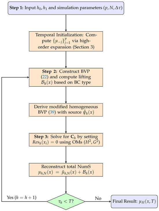
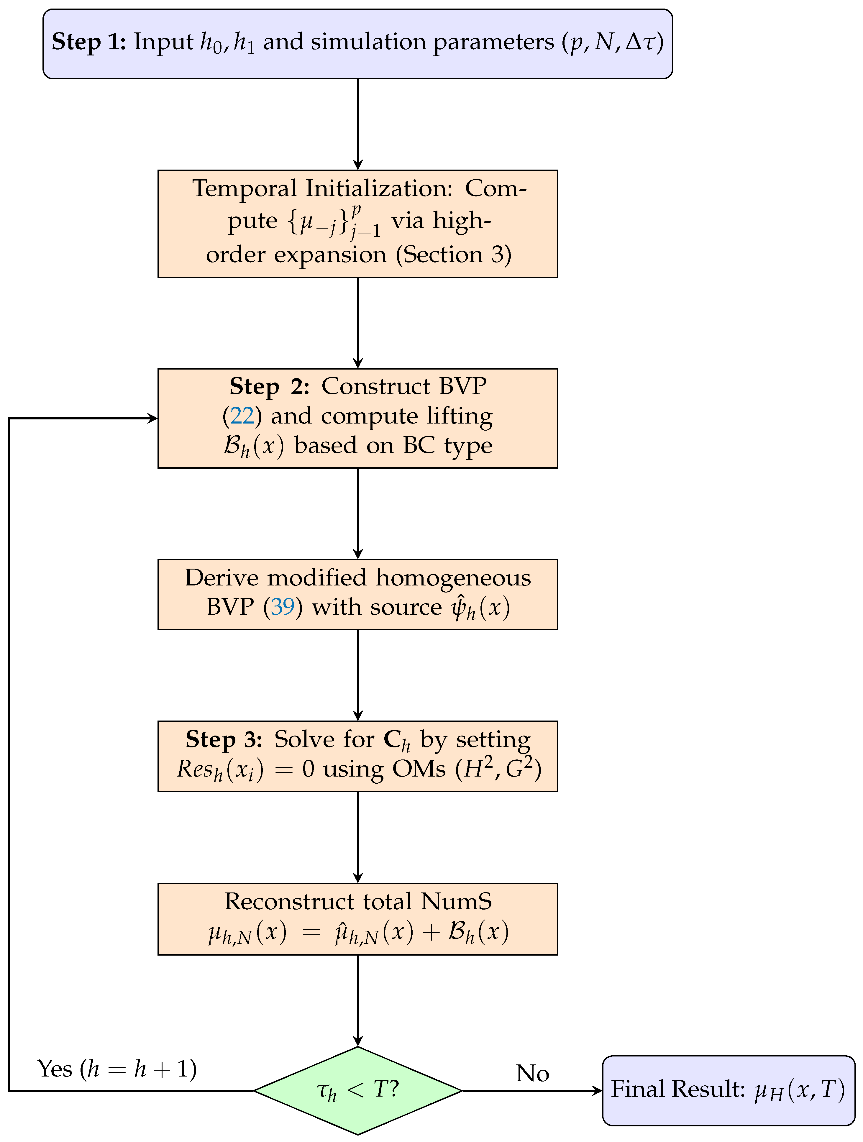
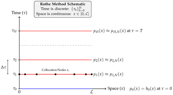
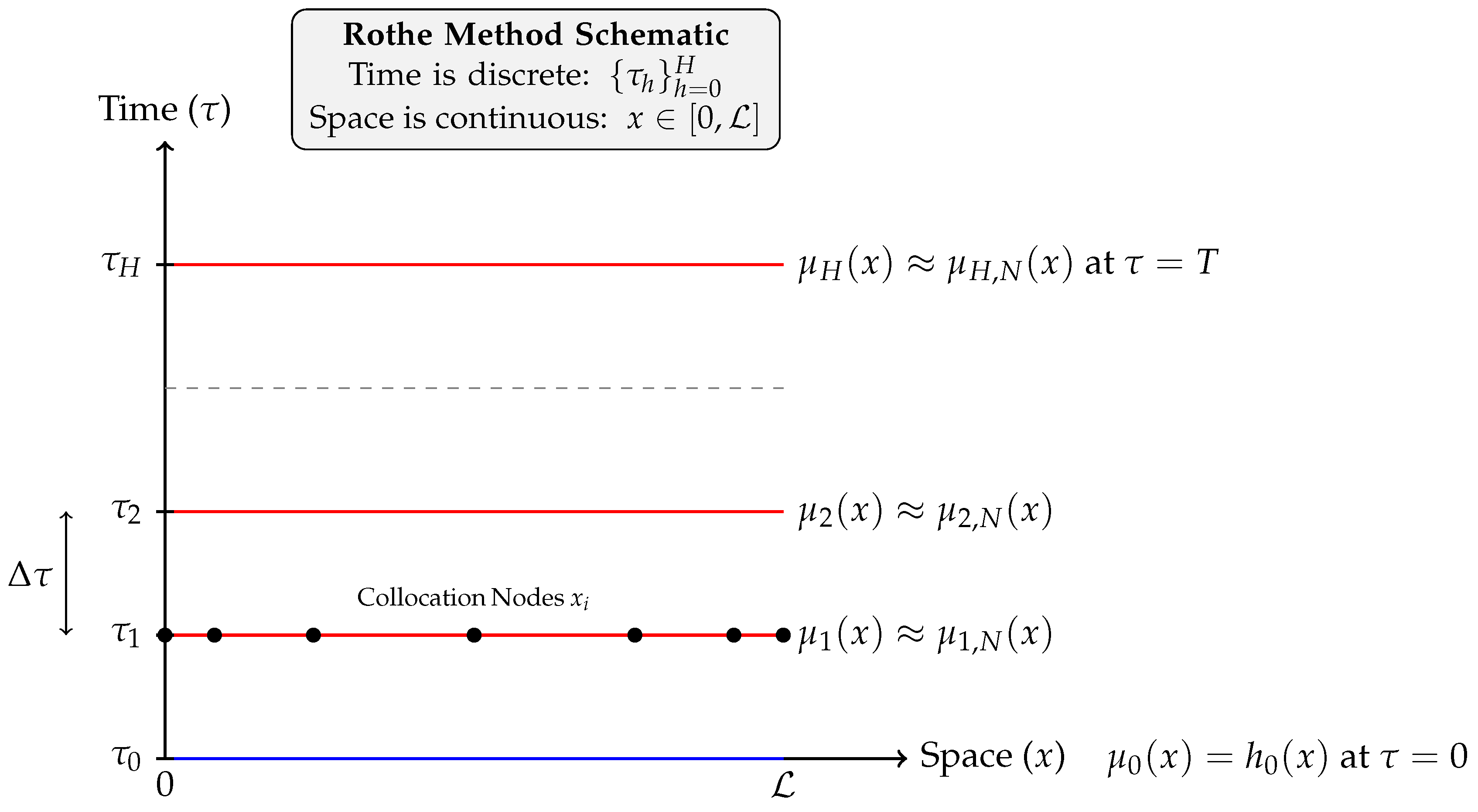
The proposed hybrid Rothe-GSJP method constitutes a systematic integration of temporal semi-discretization and spatial spectral resolution, as detailed in Figure 1 and illustrated in the schematic shown in Figure 2. The operational workflow of the proposed Rothe-GSJP framework is systematically encapsulated in Algorithm 1, which provides a rigorous step-by-step synthesis of the temporal marching scheme and the spatial collocation process.

Figure 1. Unified procedural flowchart of the high-order Rothe-GSJP algorithm handling both DBC and NBC.

Figure 2. Schematic representation of the Rothe method utilizing semi-discretization.

Algorithm 1 Rothe-GSJP algorithm to solve the telegraph equation subject to IBCs

Stage 1.       Given $\alpha ,\beta ,\mathcal{L},\mathcal{T},N,p,\Delta \tau ,a,b,c,f(x,\tau )$ and IBCs $g_0\left(\tau \right),g_1\left(\tau \right),h_0\left(x\right),h_1\left(x\right)$.

Stage 2.       For DBCs: Define the GSJP basis ${\phi }_n^{({\varrho }_1,{\varrho }_2)}\left(x\right)$ and the OMs $\mathbf{H}$ and ${\mathbf{H}}^2$.

For NBCs: Define the GSJP basis ${\psi }_{j,\mathcal{L}}^{({\varrho }_1,{\varrho }_2)}\left(x\right)$ and the OMs $\mathbf{M}$ and ${\mathbf{M}}^2$.

Stage 3.       Apply the Rothe method for TD at levels ${\tau }_h=h\Delta \tau$:

1. Approximate ${\displaystyle \frac{{\partial }^2\mu }{\partial {\tau }^2}}$ and ${\displaystyle \frac{\partial \mu }{\partial \tau }}$ using p-th-order BDF stencils.

2. Linearize the PDE into a sequence of spatial BVPs for each time step h.

Stage 4.       Initialization: For $p>1$, calculate historical levels ${\mu }_{-j}\left(x\right)$ for $j=1,\dots ,p-1$

via the Taylor expansion (30) and Lemma 1.

Stage 5.       For each time level $h=1,2,\dots ,H$:

1. Construct the boundary lifting function ${\mathcal{B}}_h\left(x\right)$ as per Equation (36).

2. Express the homogenized solution as defined in (32).

3. Define the residual $Re{s}_h\left(x\right)$ as in (34).

4. List $Re{s}_h\left(x_i\right)=0,i=0,1,\dots ,N$ as defined in (35).

5. Use Mathematica’s solver to obtain the vector ${\mathbf{C}}_h={[c_{h,0},c_{h,1},\dots ,c_{h,N}]}^T$.

6. Reconstruct the total NumS in the form:

${\mu }_{h,N}\left(x\right)=\left\{\begin{array}{cc}{\mathbf{C}}_h^T{\mathit{\phi }}_{N,\mathcal{L}}^{({\varrho }_1,{\varrho }_2)}\left(x\right)+{\mathcal{B}}_h\left(x\right),\hfill & \mathrm{for}\mathrm{DBC},\hfill \\ {\mathbf{C}}_h^T{\mathbf{\Psi }}_{N,\mathcal{L}}^{({\varrho }_1,{\varrho }_2)}\left(x\right)+{\mathcal{B}}_h\left(x\right),\hfill & \mathrm{for}\mathrm{NBC}.\hfill \end{array}\right.$

7. Store the local expansion ${\mu }_{h,N}\left(x\right)$.

Stage 6.       End For.

Stage 7.       Define the global NumS ${\mu }_{N,H}(\tau ,x)$ as defined in (42).

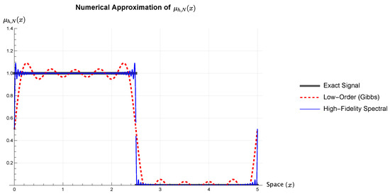
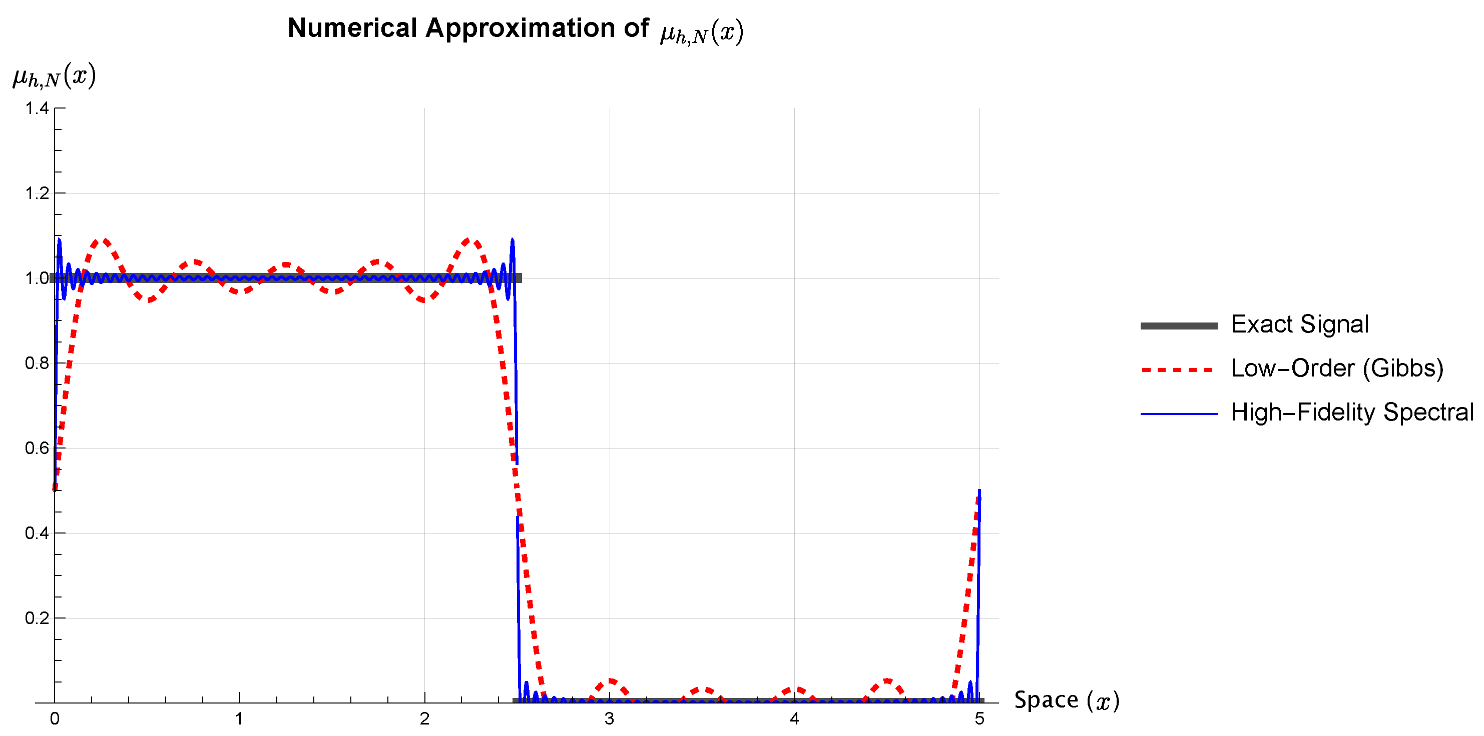
This strategy yields a non-oscillatory reconstruction at the boundaries and captures oscillatory dynamics with spectral fidelity, as shown in Figure 3. The resulting high-order reconstruction ensures a global accuracy of $\mathcal{O}({(\Delta \tau )}^p+N^{-s})$, where the spatial convergence is governed by the regularity s, as established in Section 6.

Figure 3. Comparison of the numerical approximation ${\mu }_{h,N}\left(x\right)$ on the domain $[0,\mathcal{L}]$. The high-fidelity GSJP reconstruction (solid blue line) demonstrates the absence of spurious oscillations and the superior resolution of gradients at the boundaries compared to a low-order approximation (dashed red line). The close agreement with the ExaS (thick gray line) verifies the spectral convergence rate and the stability of the hybrid scheme in capturing high-frequency oscillatory behavior.

6. Error Estimation and Convergence Analysis

In this section, we provide a rigorous theoretical investigation into the convergence properties of the hybrid Rothe-GSJP method. The global discretization error is governed by the interplay between the temporal step size $\Delta \tau$ and the spatial resolution determined by the number of basis functions N. To ensure mathematical consistency across the different discretization stages, we adopt a hybrid norm strategy: temporal consistency is established in the $L^{\infty }$ norm to guarantee uniform pointwise stability, while spatial accuracy is analyzed within the framework of weighted Sobolev spaces to leverage the spectral convergence of the GSJP basis.

We assume that the ExaS $\mu (\tau ,x)$ possesses sufficient regularity such that $\mu \in C^{p+1}([0,\mathcal{T}];H_{w_{\mathcal{L}}^{{\varrho }_1,{\varrho }_2}}^s(0,\mathcal{L}))$, where $s>2$ and p is the order of the BDF scheme. This ensures that the high-order temporal derivatives are bounded in the $L^{\infty }$ sense and that the spatial derivatives are square integrable with respect to the weight function $w_{\mathcal{L}}^{{\varrho }_1,{\varrho }_2}\left(x\right)$. Under these assumptions, we define the global discretization error at any time level ${\tau }_h$ as

$$E_{global,h,N}=\mu ({\tau }_h,x)-{\mu }_{h,N}\left(x\right).$$

(44)

This error is decomposed into the temporal and spatial components, as follows:

$$\parallel E_{global,h,N}{\parallel }_{L_{w_{\mathcal{L}}^{{\varrho }_1,{\varrho }_2}}^2}\le \underset{\mathrm{Temporal}\mathrm{Error}}{\underbrace{\parallel \mu ({\tau }_h,·)-{\mu }_h(·){\parallel }_{L_{w_{\mathcal{L}}^{{\varrho }_1,{\varrho }_2}}^2}}}+\underset{\mathrm{Spatial}\mathrm{Error}}{\underbrace{\parallel {\mu }_h(·)-{\mu }_{h,N}{(·)\parallel }_{L_{w_{\mathcal{L}}^{{\varrho }_1,{\varrho }_2}}^2}}}.$$

(45)

To facilitate the error analysis, we define the finite-dimensional approximation subspace $S_N\subset L_{w_{\mathcal{L}}^{{\varrho }_1,{\varrho }_2}}^2(0,\mathcal{L})$. Based on the boundary requirements specified in the previous sections, this subspace is spanned by the following set of basis functions:

$$S_N=\mathrm{span}{\left\{{\mathrm{{\rm Y}}}_j\left(x\right)\right\}}_{j=0}^N,\mathrm{where}{\mathrm{{\rm Y}}}_j\left(x\right)=\left\{\begin{array}{cc}{\mathit{\phi }}_{j,\mathcal{L}}^{({\varrho }_1,{\varrho }_2)}\left(x\right),\hfill & \mathrm{for}\mathrm{DBC},\hfill \\ {\mathbf{\Psi }}_{j,\mathcal{L}}^{({\varrho }_1,{\varrho }_2)}\left(x\right),\hfill & \mathrm{for}\mathrm{NBC}.\hfill \end{array}\right.$$

(46)

The NumS at any time level h, denoted by ${\mu }_{h,N}\left(x\right)$, is the unique element in $S_N$ satisfying the collocation equations.

Let ${\mathcal{P}}_N:L_w^2\to S_N$ denote the spatial orthogonal projection operator onto $S_N$, which satisfies the best approximation property:

$$\parallel \mu -{\mathcal{P}}_N{\mu \parallel }_{L_w^2}=\underset{v\in S_N}{inf}{\parallel \mu -v\parallel }_{L_w^2}.$$

(47)

We define the global error as

$$E_{N,H}(\tau ,x)=\mu (\tau ,x)-{\mu }_{N,H}(\tau ,x).$$

(48)

At a discrete time level ${\tau }_h$, the spatial error is denoted as

$$e_{h,N}\left(x\right)=\mu ({\tau }_h,x)-{\mu }_{h,N}\left(x\right).$$

(49)

The accuracy of the reconstruction is evaluated using the $L^{\infty }$ norm to ensure uniform convergence across the domain:

$$\parallel e_{h,N}{\parallel }_{\infty }=\underset{x\in [0,\mathcal{L}]}{max}|\mu ({\tau }_h,x)-{\mu }_{h,N}\left(x\right)|.$$

(50)

6.1. Temporal Error Analysis: Pointwise Consistency of the Rothe Scheme

In this subsection, we focus on the errors arising from the TD. We establish the consistency of the p-th-order generalized difference formulae by estimating the local error estimate (LEE) in the infinite norm, which ensures uniform accuracy across the spatial domain.

Lemma 2.

Assume that the ExaS $\mu (\tau ,x)$ is sufficiently smooth such that $\mu \in C^{p+1}([0,\mathcal{T}]$; $H_{w_{\mathcal{L}}^{{\varrho }_1,{\varrho }_2}}^s(0,\mathcal{L}))$, where p is the order of the BDF scheme. Further assume that the variable coefficients $a,b,c$ and the source term f are bounded and possess sufficient smoothness on the closed domain Ω. This ensures that the governing HTE remains well-posed and that the high-order BDF stencils satisfy the necessary stability and consistency conditions for long-term integration. Then, the LEE ${\epsilon }_h$ satisfies

$$\parallel {\epsilon }_h{\parallel }_{\infty }=\mathcal{O}\left({(\Delta \tau )}^{p+1}\right).$$

(51)

Proof. 

The local error estimate ${\epsilon }_h\left(x\right)$ is defined as the residual obtained by substituting the ExaS $\mu (\tau ,x)$ into the semi-discrete BVP system (22). At a fixed time level ${\tau }_h$, the residual is

$${\epsilon }_h\left(x\right)=\left[\sum _{j=0}^{p+1}{\beta }_j\mu ({\tau }_{h-j},x)\right]+2\Delta \tau a_h\left[\sum _{j=0}^{p+1}{\alpha }_j\mu ({\tau }_{h-j},x)\right]+\Delta {\tau }^2{b}_h^2\mu ({\tau }_h,x)-\Delta {\tau }^2{c}_h{\mu }_{xx}({\tau }_h,x)-\Delta {\tau }^2{f}_h\left(x\right).$$

(52)

We expand $\mu ({\tau }_{h-j},x)$ in a Taylor series about the current time level ${\tau }_h$:

$$\mu ({\tau }_{h-j},x)=\sum _{k=0}^{p+1}{\displaystyle \frac{{(-j\Delta \tau )}^k}{k!}}{\displaystyle \frac{{\partial }^k\mu ({\tau }_h,x)}{\partial {\tau }^k}}+\mathcal{O}(\Delta {\tau }^{p+2}).$$

(53)

Substituting (53) into (52) and rearranging terms by derivative order k, we obtain

$${\epsilon }_h\left(x\right)=\sum _{k=0}^{p+1}{\displaystyle \frac{{(-\Delta \tau )}^k}{k!}}\left[\sum _{j=0}^{p+1}{j}^k{\beta }_j+2\Delta \tau a_h\left(\sum _{j=0}^{p+1}{j}^k{\alpha }_j\right)\right]{\displaystyle \frac{{\partial }^k\mu }{\partial {\tau }^k}}+\Delta {\tau }^2{b}_h^2\mu -\Delta {\tau }^2{c}_h{\mu }_{xx}-\Delta {\tau }^2{f}_h.$$

(54)

The coefficients ${\alpha }_j$ and ${\beta }_j$ are BDF weights of order p. According to the consistency conditions for linear multi-step methods [28,29], these weights must satisfy specific algebraic properties to nullify the lower-order terms of the Taylor expansion. These properties are given by

$$\sum _{j=0}^{p+1}{j}^k{\alpha }_j=\left\{\begin{array}{cc}0,\hfill & k=0\hfill \\ -1,\hfill & k=1\hfill \\ 0,\hfill & 2\le k\le p\hfill \end{array}\right.,\sum _{j=0}^{p+1}{j}^k{\beta }_j=\left\{\begin{array}{cc}0,\hfill & k=0,1\hfill \\ 2,\hfill & k=2\hfill \\ 0,\hfill & 3\le k\le p\hfill \end{array}\right..$$

(55)

By applying (55) to (54) for $k=0,1,2$, we evaluate the following:

• For $k=0$, ${\displaystyle \frac{{(-\Delta \tau )}^0}{0!}}[0+2\Delta \tau a_h\left(0\right)]\mu =0$.
• For $k=1$, ${\displaystyle \frac{{(-\Delta \tau )}^1}{1!}}[0+2\Delta \tau a_h(-1)]{\mu }_{\tau }=2{(\Delta \tau )}^2{a}_h{\mu }_{\tau }$.
• For $k=2$, ${\displaystyle \frac{{(-\Delta \tau )}^2}{2!}}[2+2\Delta \tau a_h\left(0\right)]{\mu }_{\tau \tau }={(\Delta \tau )}^2{\mu }_{\tau \tau }$.

In view of these properties, the terms in (54) for $k\le p$ simplify and combine with the remaining spatial and source terms to form the exact governing equation. Since the ExaS satisfies (1), these terms vanish identically:

$${\epsilon }_h\left(x\right)=\Delta {\left(\tau \right)}^2\underset{=0}{\underbrace{\left[{\displaystyle \frac{{\partial }^2\mu }{\partial {\tau }^2}}+2a_h{\displaystyle \frac{\partial \mu }{\partial \tau }}+b_h^2\mu -c_h{\mu }_{xx}-f_h\right]}}+\mathrm{Remainder}\mathrm{Terms}.$$

(56)

The first non-vanishing term in the Taylor expansion occurs at $k=p+1$. In view of (55), the local error is governed by

$${\epsilon }_h\left(x\right)={\displaystyle \frac{{(-\Delta \tau )}^{p+1}}{(p+1)!}}\left[\sum _{j=0}^{p+1}{j}^{p+1}{\beta }_j+2\Delta \tau a_h\sum _{j=0}^{p+1}{j}^{p+1}{\alpha }_j\right]{\displaystyle \frac{{\partial }^{p+1}\mu }{\partial {\tau }^{p+1}}}+\mathcal{O}(\Delta {\tau }^{p+2}).$$

(57)

Since the term involved ${\alpha }_j$ is scaled by an additional $\Delta \tau$, it is $\mathcal{O}\left({(\Delta \tau )}^{p+2}\right)$. Thus, the leading order of the local error is determined by the ${\beta }_j$ summation:

$${\epsilon }_h\left(x\right)={(\Delta \tau )}^{p+1}\left[{\displaystyle \frac{{(-1)}^{p+1}}{(p+1)!}}\sum _{j=0}^{p+1}{j}^{p+1}{\beta }_j\right]{\displaystyle \frac{{\partial }^{p+1}\mu }{\partial {\tau }^{p+1}}}+\mathcal{O}(\Delta {\tau }^{p+2}).$$

(58)

Taking the ${\mathcal{L}}_{\infty }$-norm over $x\in [0,\mathcal{L}]$ and utilizing the boundedness of the temporal derivatives, we conclude that

$$\parallel {\epsilon }_h{\parallel }_{\infty }\le \mathcal{C}{(\Delta \tau )}^{p+1}=\mathcal{O}\left({(\Delta \tau )}^{p+1}\right).$$

(59)

This completes the proof. □

Remark 2.

The consistency established in Lemma 2 relies on the structural stability of the variable coefficients $a(x,\tau )$, $b^2(x,\tau )$, and $c(x,\tau )$. In physical systems such as PLL modeling, these parameters represent space–time-dependent damping and propagation speeds [2,15]. By assuming these functions are bounded and sufficiently smooth, we ensure that the local truncation error does not experience non-physical amplification during the temporal marching process. This theoretical assumption is numerically validated in Section 7, where the algorithm maintains a stable ${10}^{-16}$ precision floor across all test cases.

6.2. Spatial Error Analysis: Spectral Approximation in Weighted Sobolev Spaces

In the following theorem, we utilize the weighted Sobolev space $H_{\omega ,N}^s(0,\mathcal{L})$ to quantify the regularity of the solution and the accuracy of the approximation. For any $s\ge 0$, the full weighted Sobolev norm ${\parallel \mu \parallel }_{H_{\omega ,N}^s}$ is defined as the square root of the sum of the weighted $L^2$-norms of the function and its derivatives up to order s [12]:

$${\parallel \mu \parallel }_{H_{\omega ,N}^s}={\left(\sum _{i=0}^s{\int }_0^{\mathcal{L}}{\left|{\displaystyle \frac{d^i\mu \left(x\right)}{d{x}^i}}\right|}^2{\omega }_{\mathcal{L}}^{{\varrho }_1+i,{\varrho }_2+i}\left(x\right)dx\right)}^{1/2},$$

(60)

where ${\omega }_{\mathcal{L}}^{{\varrho }_1+i,{\varrho }_2+i)}\left(x\right)$ denotes the shifted Jacobi weight function corresponding to the i-th derivative.

Lemma 3

([12]). Let ${\mathcal{I}}_N$ be the polynomial interpolation operator at the Jacobi–Gauss-type nodes associated with the weight $w_{\mathcal{L}}^{{\varrho }_1,{\varrho }_2}$. For any $\mu \in H_{w_{\mathcal{L}}^{{\varrho }_1,{\varrho }_2}}^s(0,\mathcal{L})$, the interpolation error is bounded by the projection error as follows:

$$\parallel \mu -{\mathcal{I}}_N{\mu \parallel }_{L_{w_{\mathcal{L}}^{{\varrho }_1,{\varrho }_2}}^2}\le (1+{\mathrm{\Lambda }}_N){\parallel \mu -{\mathcal{P}}_N\mu \parallel }_{L_{w_{\mathcal{L}}^{{\varrho }_1,{\varrho }_2}}^2},$$

(61)

where the Lebesgue constant ${\mathrm{\Lambda }}_N$ satisfies the asymptotic growth ${\mathrm{\Lambda }}_N\sim \mathcal{O}(logN)$ [30].

Theorem 3.

Let $s\in {\mathbb{Z}}^{+}$ be an integer such that $s\ge 2$. Suppose that at any discrete time level h, the semi-discrete solution ${\mu }_h$ belongs to the weighted Sobolev space $H_{w_{\mathcal{L}}^{{\varrho }_1,{\varrho }_2}}^s(0,\mathcal{L})$. The spatial discretization error for the GSJP-based collocation approximation ${\mu }_{h,N}$ satisfies

$$\parallel {\epsilon }_{h,N}{\parallel }_{L_{w_{\mathcal{L}}^{{\varrho }_1,{\varrho }_2}}^2}=\parallel {\mu }_h-{\mu }_{h,N}{\parallel }_{L_{w_{\mathcal{L}}^{{\varrho }_1,{\varrho }_2}}^2}\le C{N}^{-s}{\parallel {\mu }_h\parallel }_{H_{w_{\mathcal{L}}^{{\varrho }_1,{\varrho }_2}}^s},$$

(62)

where C is a positive constant independent of N.

Proof. 

Utilizing the orthogonal projection operator ${\mathcal{P}}_N$ onto the subspace $S_N$ defined in (46), we apply the triangle inequality to decompose the error as follows:

$$\parallel {\epsilon }_{h,N}{\parallel }_{L_{w_{\mathcal{L}}^{{\varrho }_1,{\varrho }_2}}^2}={\parallel {\mu }_h-{\mu }_{h,N}\parallel }_{L_{w_{\mathcal{L}}^{{\varrho }_1,{\varrho }_2}}^2}\le \underset{\mathrm{Term}\mathrm{I}}{\underbrace{\parallel {\mu }_h-{\mathcal{P}}_N{\mu }_h{\parallel }_{L_{w_{\mathcal{L}}^{{\varrho }_1,{\varrho }_2}}^2}}}+\underset{\mathrm{Term}\mathrm{II}}{\underbrace{\parallel {\mathcal{P}}_N{\mu }_h-{\mu }_{h,N}{\parallel }_{L_{w_{\mathcal{L}}^{{\varrho }_1,{\varrho }_2}}^2}}}.$$

(63)

Term I represents the projection error in the weighted Hilbert space. According to the spectral approximation theory for Jacobi-type polynomials in weighted Sobolev spaces (see [12,31]), for ${\mu }_h\in H_{w_{\mathcal{L}}^{{\varrho }_1,{\varrho }_2}}^s(0,\mathcal{L})$ with $s\ge 2$, there exists a positive constant $C_1$ independent of N such that

$$\parallel {\mu }_h-{\mathcal{P}}_N{\mu }_h{\parallel }_{L_{w_{\mathcal{L}}^{{\varrho }_1,{\varrho }_2}}^2}\le C_1{N}^{-s}{\parallel {\mu }_h\parallel }_{H_{w_{\mathcal{L}}^{{\varrho }_1,{\varrho }_2}}^s}.$$

(64)

For Term II, we evaluate the departure of the collocation solution ${\mu }_{h,N}$ from the orthogonal projection. Since ${\mu }_{h,N}$ is the spectral expansion satisfying the collocation conditions at the Jacobi–Gauss-type nodes, it is equivalent to the polynomial interpolant ${\mathcal{I}}_N{\mu }_h$. This leads to the following inequality:

$$\parallel {\mathcal{P}}_N{\mu }_h-{\mu }_{h,N}{\parallel }_{L_{w_{\mathcal{L}}^{{\varrho }_1,{\varrho }_2}}^2}=\parallel {\mathcal{P}}_N{\mu }_h-{\mathcal{I}}_N{\mu }_h{\parallel }_{L_{w_{\mathcal{L}}^{{\varrho }_1,{\varrho }_2}}^2}\le \parallel {\mathcal{P}}_N{\mu }_h-{\mu }_h{\parallel }_{L_{w_{\mathcal{L}}^{{\varrho }_1,{\varrho }_2}}^2}+{\parallel {\mu }_h-{\mathcal{I}}_N{\mu }_h\parallel }_{L_{w_{\mathcal{L}}^{{\varrho }_1,{\varrho }_2}}^2}.$$

(65)

By invoking Lemma 3, the interpolation error is bounded by the projection error magnified by the Lebesgue constant ${\mathrm{\Lambda }}_N$:

$$\parallel {\mu }_h-{\mathcal{I}}_N{\mu }_h{\parallel }_{L_{w_{\mathcal{L}}^{{\varrho }_1,{\varrho }_2}}^2}\le (1+{\mathrm{\Lambda }}_N){\parallel {\mu }_h-{\mathcal{P}}_N{\mu }_h\parallel }_{L_{w_{\mathcal{L}}^{{\varrho }_1,{\varrho }_2}}^2}.$$

(66)

Substituting (66) into (65) leads to the bound for Term II:

$$\parallel {\mathcal{P}}_N{\mu }_h-{\mu }_{h,N}{\parallel }_{L_{w_{\mathcal{L}}^{{\varrho }_1,{\varrho }_2}}^2}\le (2+{\mathrm{\Lambda }}_N){\parallel {\mu }_h-{\mathcal{P}}_N{\mu }_h\parallel }_{L_{w_{\mathcal{L}}^{{\varrho }_1,{\varrho }_2}}^2}.$$

(67)

Finally, substituting (64) into (67) and the result back into (63), we obtain

$$\parallel {\epsilon }_{h,N}{\parallel }_{L_{w_{\mathcal{L}}^{{\varrho }_1,{\varrho }_2}}^2}\le C_1(3+{\mathrm{\Lambda }}_N)N^{-s}{\parallel {\mu }_h\parallel }_{H_{w_{\mathcal{L}}^{{\varrho }_1,{\varrho }_2}}^s}.$$

(68)

Since ${\mathrm{\Lambda }}_N\sim \mathcal{O}(logN)$, the product $(3+{\mathrm{\Lambda }}_N)N^{-s}$ is asymptotically dominated by the algebraic decay rate $N^{-s}$. Thus, there exists a consolidated constant C such that

$$\parallel {\epsilon }_{h,N}{\parallel }_{L_{w_{\mathcal{L}}^{{\varrho }_1,{\varrho }_2}}^2}\le C{N}^{-s}{\parallel {\mu }_h\parallel }_{H_{w_{\mathcal{L}}^{{\varrho }_1,{\varrho }_2}}^s}.$$

(69)

This confirms the spectral convergence of the spatial discretization, completing the proof. □

6.3. Global Convergence: The Unified Fully Discrete Error Estimate

In the preceding subsections, the temporal and spatial discretization errors were investigated in isolation to establish their respective rates of consistency. However, the practical utility of the hybrid Rothe-GSJP method depends on the accumulated global error, where temporal stability and spatial approximation interact simultaneously. The purpose of this subsection is to consolidate the local estimates from Lemma 2 and Theorem 3 into a single, unified convergence theorem. By employing a triangle inequality decomposition within the weighted Hilbert space $L_{w_{\mathcal{L}}^{{\varrho }_1,{\varrho }_2}}^2$, we demonstrate that the global error $E_{global,H,N}$ is bounded by the sum of the p-th-order algebraic decay in time and the spectral decay in space. This analysis provides the theoretical guarantee that the NumS converges to the ExaS of the HTE as the discretization parameters are refined.

Theorem 4.

Let $\mu (\tau ,·)$ be the ExaS of the HTE (1) and ${\mu }_{N,H}(\tau ,·)$ be the NumS obtained via the hybrid Rothe-GSJP method. Under the assumption of a p-th-order temporal BDF and spatial regularity $s\ge 2$, the global discretization error at the final time T satisfies

$$\parallel E_{global,H,N}{\parallel }_{L_{w_{\mathcal{L}}^{{\varrho }_1,{\varrho }_2}}^2}\le C_1{(\Delta \tau )}^p+C_2{N}^{-s}{\parallel \mu \parallel }_{H_{w_{\mathcal{L}}^{{\varrho }_1,{\varrho }_2}}^s},1\le p\le 6,s\ge 2,$$

(70)

where $C_1$ is a constant independent of $\Delta \tau$ related to the temporal stability of the Rothe scheme, and $C_2$ is a constant independent of N associated with the spatial spectral accuracy.

Proof. 

Let $E_{global,h,N}(·)=\mu ({\tau }_h,·)-{\mu }_{h,N}(·)$ denote the global error at the h-th time step. By applying the triangle inequality, the total error is decomposed into temporal and spatial components:

$$\parallel E_{global,h,N}{\parallel }_{L_{w_{\mathcal{L}}^{{\varrho }_1,{\varrho }_2}}^2}\le \underset{\mathrm{Temporal}\mathrm{Error}}{\underbrace{\parallel \mu ({\tau }_h,·)-{\mu }_h(·){\parallel }_{L_{w_{\mathcal{L}}^{{\varrho }_1,{\varrho }_2}}^2}}}+\underset{\mathrm{Spatial}\mathrm{Error}}{\underbrace{\parallel {\mu }_h(·)-{\mu }_{h,N}{(·)\parallel }_{L_{w_{\mathcal{L}}^{{\varrho }_1,{\varrho }_2}}^2}}},$$

(71)

where ${\mu }_h$ is the semi-discrete solution obtained after TD but before spatial approximation.

The temporal error in (71) arises from the accumulation of local truncation errors ${\epsilon }_h$ over $H=T/\Delta \tau$ time steps. According to Lemma 2, the local truncation error is $\parallel {\epsilon }_h{\parallel }_{\infty }=\mathcal{O}\left({(\Delta \tau )}^{p+1}\right)$. Since BDF methods of order $p\le 6$ are zero stable for second-order evolution equations [29], the Lax Equivalence Theorem [29] implies that the accumulated global temporal error at any ${\tau }_h\le T$ satisfies

$$\parallel \mu ({\tau }_h,·)-{\mu }_h(·){\parallel }_{L_{w_{\mathcal{L}}^{{\varrho }_1,{\varrho }_2}}^2}\le \sum _{j=1}^h\parallel {\epsilon }_j\parallel \le C_1{(\Delta \tau )}^p,$$

(72)

where $C_1$ depends on the higher-order temporal derivatives of the ExaS.

The spatial error in (71) accounts for the discretization error at time level h, denoted by $\parallel {\epsilon }_{h,N}{\parallel }_{L_{w_{\mathcal{L}}^{{\varrho }_1,{\varrho }_2}}^2}$. As demonstrated in Theorem 3, the GSJP-based collocation method yields spectral convergence. For ${\mu }_h\in H_{w_{\mathcal{L}}^{{\varrho }_1,{\varrho }_2}}^s(0,\mathcal{L})$, the following estimate holds:

$$\parallel {\mu }_h(·)-{\mu }_{h,N}{(·)\parallel }_{L_{w_{\mathcal{L}}^{{\varrho }_1,{\varrho }_2}}^2}\le C_2{N}^{-s}{\parallel {\mu }_h\parallel }_{H_{w_{\mathcal{L}}^{{\varrho }_1,{\varrho }_2}}^s}.$$

(73)

Substituting (72) and (73) into (71) yields the combined bound. Evaluating the expression at the final time step ${\tau }_H=T$ and noting that $\parallel {\mu }_h{\parallel }_{H_w^s}\to {\parallel \mu \parallel }_{H_w^s}$ as $\Delta \tau \to 0$, we obtain

$$\parallel E_{global,H,N}{\parallel }_{L_{w_{\mathcal{L}}^{{\varrho }_1,{\varrho }_2}}^2}\le C_1{(\Delta \tau )}^p+C_2{N}^{-s}{\parallel \mu \parallel }_{H_{w_{\mathcal{L}}^{{\varrho }_1,{\varrho }_2}}^s}.$$

(74)

Since the stability of the BDF scheme ensures the constants remain bounded over the finite interval $[0,T]$, the NumS converges to the ExaS at the predicted rates. This completes the proof. □

Remark 3.

The constraint $p\le 6$ in Theorem 4 is fundamental, as BDF methods are zero stable only within this range. For $p>6$, the schemes are inherently unstable and fail to satisfy the Lax Equivalence Theorem requirements for long-term integration. In the context of the HTE, numerical evidence suggests that $p\in \{2,3,4\}$ provides the most robust balance between high-order temporal precision and a favorable region of absolute stability [29].

Remark 4.

The theoretical bound established in Theorem 4 is derived in the weighted Hilbert space $L_{w_{\mathcal{L}}^{{\varrho }_1,{\varrho }_2}}^2$, yet the numerical experiments in Section 7 are reported using the ${\mathcal{L}}_{\infty }$ norm. This transition is justified by two primary factors:

1.

Sobolev Embedding: For a regularity index $s>1/2$, the continuous embedding $H_w^s\hookrightarrow C[0,\mathcal{L}]$ ensures that the spectral decay proven in the mean square sense is inherited pointwise across the entire closed interval, such that

$$\parallel E_{N,H}{\parallel }_{\infty }\le \mathcal{C}{\parallel E_{N,H}\parallel }_{H_w^s}\le \mathcal{O}({(\Delta \tau )}^p+N^{-s}).$$

(75)

2.

Structural Satisfaction of BCs: Because the GSJP basis satisfies the HBCs exactly by construction, the error at the boundaries is structurally zero. Consequently, the ${\mathcal{L}}_{\infty }$ results in Section 7 rigorously verify the interior reconstruction accuracy and confirm the absence of order reduction or Gibbs oscillations.

This theoretical framework provides the foundation for the high-precision results demonstrated in the following section.

6.4. Summary of Convergence Analysis

In this section, we have rigorously established the convergence properties of the hybrid Rothe-GSJP scheme. The proof is built upon two fundamental pillars: first, Lemma 2 establishes a local temporal truncation error of $\mathcal{O}\left({(\Delta \tau )}^{p+1}\right)$; second, Theorem 3 proves that the spatial discretization, utilizing the GSJP basis, yields spectral convergence $\mathcal{O}\left(N^{-s}\right)$ in weighted Sobolev spaces. By synthesizing these results under the framework of the Lax Equivalence Theorem and ensuring zero stability through the constraint $1\le p\le 6$, we arrive at Theorem 4. This theorem provides the unified global bound, as follows:

$$\mathcal{O}({(\Delta \tau )}^p+N^{-s}),1\le p\le 6,s\ge 2,$$

This theoretical foundation guarantees that the Rothe-GSJP method can reach the ${10}^{-16}$ machine precision floor, a claim we verify through the numerical experiments in the following section.

7. Numerical Simulations and Discussion

In this section, we present three numerical experiments to validate the theoretical findings established in the preceding sections. The primary objective is to demonstrate the p-th-order temporal convergence and the spectral spatial accuracy of the proposed Rothe-GSJP method across various test cases.

The numerical computations were performed using Mathematica 13.3 on a workstation equipped with an Intel(R) Core(TM) i9-10850 CPU operating at 3.60 GHz, featuring ten cores and 20 logical processors, supported by 64 GB of RAM. This computational environment ensures the high-precision symbolic and numerical evaluation of the BDF weights ${\alpha }_j,{\beta }_j$ and the GSJP basis functions.

As justified in Remark 4, the performance of the algorithm is assessed primarily through the maximum error ${\mathcal{L}}_{\infty }$, which provides the most stringent verification of the method’s ability to reach the machine precision floor. Where relevant for comparative purposes, the standard ${\mathcal{L}}_2$ norm is also reported. In all cases, the numerical results align with the theoretical global error bound $\parallel E_{N,H}{\parallel }_{\infty }=\mathcal{O}({(\Delta \tau )}^p+N^{-s})$.

7.1. Test Case 7.1

In this initial benchmark, we consider the HTE (1) with the following coefficient functions and non-homogeneous source term as specified in [15] (Test Case 5.1):

$$a(x,\tau )={\displaystyle \frac{1}{2}},b^2(x,\tau )=1,c(x,\tau )=1,f(x,\tau )=1-\tau +x^2.$$

(76)

Substituting these parameters into the governing equation for, we obtain

$${\displaystyle \frac{{\partial }^2\mu }{\partial {\tau }^2}}+{\displaystyle \frac{\partial \mu }{\partial \tau }}+\mu ={\displaystyle \frac{{\partial }^2\mu }{\partial x^2}}+1-\tau +x^2,(x,\tau )\in (0,1]\times (0,1).$$

(77)

This equation comes with the following ICs:

$$\mu (x,0)=x^2,{\displaystyle \frac{\partial \mu }{\partial \tau }}(x,0)=1,x\in [0,1],$$

(78)

and the following DBCs:

$$\mu (0,\tau )=\tau ,\mu (1,\tau )=1+\tau ,\tau \in [0,1],$$

(79)

It is verified that the analytical solution for this case is

$$\mu (x,\tau )=\tau +x^2.$$

(80)

We employ the second-order BDF ($p=2$) for the TD. However, because the ExaS $\mu (\tau ,x)=\tau +x^2$ is linear with respect to $\tau$, the second-order temporal derivative is exactly zero. Consequently, any p-th-order approximation for $p\ge 1$ would recover the temporal derivatives without a truncation error, rendering the time stepping process symbolically exact.

Applying the TD at time levels ${\tau }_h=h\Delta \tau$ for $h=1,2,\dots ,H$, we obtain a sequence of spatial BVPs in the form

$${\mu }_h^{″}\left(x\right)-{\mu }_h\left(x\right)={\tau }_h-x^2,{\mu }_h\left(0\right)={\tau }_h,{\mu }_h\left(1\right)={\tau }_h+1,$$

(81)

where the ExaSs of these BVPs has the form ${\mu }_h\left(x\right)=x^2+{\tau }_h$. Utilizing the boundary transformation detailed in Section 5.2 leads to

$${\tau }_h^2{\widehat{\mu }}_h^{″}\left(x\right)-{\mathrm{\Theta }}_h{\widehat{\mu }}_h\left(x\right)=2{\tau }_h^2-{\mathrm{\Theta }}_h(x^2-x),{\widehat{\mu }}_h\left(0\right)={\widehat{\mu }}_h\left(1\right)=0,$$

(82)

where ${\mathrm{\Theta }}_h=h^2+h{\tau }_h+{\tau }_h^2$ and ${\mu }_h\left(x\right)={\widehat{\mu }}_h\left(x\right)+{\mathcal{B}}_h\left(x\right)$, ${\mathcal{B}}_h\left(x\right)={\tau }_h+x$. So, ${\widehat{\mu }}_h\left(x\right)=x^2-x$.

• Applying Rothe-GSJP with $N=0$, we obtain

$${\widehat{\mu }}_h\left(x\right)={\widehat{\mu }}_{h,0}\left(x\right)=c_{h,0}·{\phi }_{1,0}^{({\varrho }_1,{\varrho }_2)}\left(x\right)=x^2-x,c_{h,0}=-1,$$

(83)

and then

$${\mu }_{h,0}\left(x\right)={\widehat{\mu }}_{h,0}\left(x\right)+{\mathcal{B}}_h\left(x\right)=x^2+{\tau }_h,h=1,2,\dots ,H,$$

(84)

which are the ExaSs ${\mu }_h\left(x\right)$ of the BVPs (81), $h=1,2,\dots ,H$.

Then, the global approximation ${\mu }_{0,H}(\tau ,x)$ over the domain $\Omega =[0,1]\times [0,1]$ is defined as follows:

$${\mu }_{0,H}(x,\tau )=\left\{\begin{array}{cc}{x}^2,\hfill & \tau =0,\hfill \\ x^2+{\tau }_h,\hfill & \tau \in ({\tau }_{h-1},{\tau }_h],h=1,2,\dots ,H.\hfill \end{array}\right.$$

(85)

7.2. Discussion of Test Case 7.1

The primary objective here is to evaluate the performance of the Rothe-GSJP method when the solution of the HTE is a polynomial in both variables. For this case, we employ BDF ($p=2$) for TD. Given that the ExaS $\mu (\tau ,x)=\tau +x^2$ is linear in $\tau$, the TD error is identically zero, allowing us to isolate the spatial performance of the GSJP-based solver.

A critical advantage of this approach, when compared to the numerical results reported in [15] (Test Case 5.1), is its handling of the modified spatial equation. While traditional solvers—such as those utilizing finite difference or standard collocation—produce numerical approximations that converge as $\Delta \tau \to 0$, the Rothe-GSJP method utilizes the boundary lifting technique to map the problem into a sequence of homogeneous spatial BVPs.

In [15], the derived AppSs for this benchmark at various time steps were recovered with high precision, yet they remained numerical approximations containing minute residuals. For instance, the solutions reported at specific time levels were

$$\begin{array}{c}\hfill {\mathcal{U}}_{2,2}\left(x\right)=1.0x^2+1.02191\times {10}^{-107}x+0.2,{\mathcal{U}}_{10,2}\left(x\right)=1.0x^2+1.48177\times {10}^{-106}x+1.0,\end{array}$$

where the residuals obtained at ${\tau }_2$ and ${\tau }_{10}$ are $1.02191\times {10}^{-107}$ and $1.48177\times {10}^{-106}$, respectively, while the residual in the Rothe-GSJP method is zero. To highlight the distinction between these high-precision numerical results and our developed algorithm, a comparative summary is provided in Table 1.

Table 1. Comparative analysis of the Rothe-GSJP method against the Rothe-SMCPs method [15] for Test Case 7.1.

Comparison Factor	Rothe-SMCPs Method [15]	Rothe-GSJP Method
Mathematical Nature	Numerical Approximation	Symbolic ExaS
Boundary Residual	Minute residual (≈${10}^{-106}$)	Structural Zero (Exact)
Expansion Resolution	$R=2$ terms	$N=0$ (Single basis function)
Temporal Accuracy	Truncation-dependent	Algebraically Exact

In contrast, the current method identifies the required expansion coefficient exactly as $c_{h,0}=-1$ for the solution of the modified BVPs (82) at each discrete time level ${\tau }_h$. The resulting expression (83) provides the exact homogeneous part, which combines with the LF ${\mathcal{B}}_h\left(x\right)={\tau }_h+x$ to yield the total solution (84). This result constitutes the exact symbolic solution of the spatial BVPs (81) at the specified time levels. It is worth noting that while traditional spectral methods often require a high number of basis functions to reach high precision, the modified equation approach used in the Rothe-GSJP method reduces the complexity of the residual so significantly that a single basis function ($N=0$) captures the entire spatial dynamics identically.

7.3. Test Case 7.2

In this case, we consider the HTE (1) with constant coefficients and a homogeneous source function as specified in [15] (Test Case 5.2):

$$a(x,\tau )=3,b^2(x,\tau )=3,c(x,\tau )=1,f(x,\tau )=0.$$

(86)

Then, the governing equation becomes

$${\displaystyle \frac{{\partial }^2\mu }{\partial {\tau }^2}}+6{\displaystyle \frac{\partial \mu }{\partial \tau }}+3\mu ={\displaystyle \frac{{\partial }^2\mu }{\partial x^2}},(\tau ,x)\in (0,5]\times (0,1).$$

(87)

This equation is accompanied by the following ICs:

$$\mu (x,0)=sinh\left(x\right),{\displaystyle \frac{\partial \mu }{\partial \tau }}(x,0)=-2sinhx,x\in [0,1],$$

(88)

and following the DBCs:

$$\mu (0,\tau )=0,\mu (1,\tau )=sinh\left(1\right)e^{-2\tau },\tau \in [0,5].$$

(89)

The analytical ExaS for this case has the form

$$\mu (x,\tau )=e^{-2\tau }sinhx.$$

(90)

7.4. Numerical Results for Test Case 7.2

In this subsection, we evaluate the performance of the Roth-GSJP framework for Test Case 7.2 across varying spatial resolutions N and temporal orders p. The investigation is conducted using the GSJP framework, which encompasses Shifted Chebyshev and Legendre bases as special cases by selecting appropriate Jacobi parameters to demonstrate the framework’s versatility. Initially, we examine the ${\mathcal{L}}_{\infty }$ error at a fixed time step $\Delta \tau =0.1$ to identify the spectral convergence of the spatial discretization and the subsequent temporal accuracy floors. This is followed by a dedicated temporal refinement study at $N=5$, which serves to independently verify the Rate of Convergence (ROC) for each BDF scheme at both the early ($\tau =1$) and late ($\tau =5$) time stages.

To verify the temporal accuracy, the empirical ROC is computed using the ratio of ${\mathcal{L}}_{\infty }$ errors obtained from two successive time step sizes, $\Delta \tau$ and $\Delta \tau /2$, as follows:

$$\mathrm{ROC}\approx {\displaystyle \frac{log\left(\mathrm{Error}\right(\Delta \tau )/\mathrm{Error}(\Delta \tau /2\left)\right)}{log\left(2\right)}}.$$

The numerical results in Table 2 and Table 3 illustrate that the Roth-GSJP framework achieves rapid spectral spatial convergence, with the ${\mathcal{L}}_{\infty }$ error reaching a saturation floor by $N=3$ or $N=4$ across the various GSJPs bases. Once this spatial saturation occurs, the total error is strictly governed by the TD order p, where transitioning from $p=1$ to $p=4$ reduces the error floor by several orders of magnitude, effectively bypassing the temporal bottlenecks common in lower-order schemes. Furthermore, the consistency between the results at the early ($\tau =1$) and late ($\tau =5$) time stages, characterized by stable error floors and expected linear error growth, confirms the long-term stability and robustness of the framework for solving the HTE.

Table 2. ${\mathcal{L}}_{\infty }$ error and CPU time (s) for Roth-GSJP at $\tau =1,\Delta \tau =0.1$ across various $p,N,$ and $({\varrho }_1,{\varrho }_2)$ for Test Case 7.2.

$({\mathit{\varrho }}_1,{\mathit{\varrho }}_2)$	p	Data	$\mathit{N}=0$	$\mathit{N}=1$	$\mathit{N}=2$	$\mathit{N}=3$	$\mathit{N}=4$	$\mathit{N}=5$
($-0.5,-0.5$)	1	${\mathcal{L}}_{\infty }$	$8.50\times {10}^{-2}$	$1.62\times {10}^{-4}$	$3.16\times {10}^{-9}$	$1.68\times {10}^{-9}$	$1.68\times {10}^{-9}$	$1.68\times {10}^{-9}$
(Chebyshev)		CPU (s)	0.022	0.044	0.069	0.082	0.102	0.123
	2	${\mathcal{L}}_{\infty }$	$8.50\times {10}^{-2}$	$1.62\times {10}^{-4}$	$6.90\times {10}^{-10}$	$4.21\times {10}^{-11}$	$4.21\times {10}^{-11}$	$4.21\times {10}^{-11}$
		CPU (s)	0.023	0.047	0.070	0.086	0.105	0.127
	3	${\mathcal{L}}_{\infty }$	$8.50\times {10}^{-2}$	$1.62\times {10}^{-4}$	$6.90\times {10}^{-10}$	$1.05\times {10}^{-12}$	$1.05\times {10}^{-12}$	$1.05\times {10}^{-12}$
		CPU (s)	0.024	0.050	0.074	0.091	0.110	0.132
	4	${\mathcal{L}}_{\infty }$	$8.50\times {10}^{-2}$	$1.62\times {10}^{-4}$	$6.90\times {10}^{-10}$	$2.63\times {10}^{-14}$	$2.63\times {10}^{-14}$	$2.63\times {10}^{-14}$
		CPU (s)	0.025	0.053	0.077	0.097	0.113	0.139
($0,0$)	1	${\mathcal{L}}_{\infty }$	$1.02\times {10}^{-1}$	$1.91\times {10}^{-4}$	$4.22\times {10}^{-9}$	$1.68\times {10}^{-9}$	$1.68\times {10}^{-9}$	$1.68\times {10}^{-9}$
(Legendre)		CPU (s)	0.022	0.043	0.068	0.081	0.101	0.122
	2	${\mathcal{L}}_{\infty }$	$1.02\times {10}^{-1}$	$1.91\times {10}^{-4}$	$1.05\times {10}^{-9}$	$4.21\times {10}^{-11}$	$4.21\times {10}^{-11}$	$4.21\times {10}^{-11}$
		CPU (s)	0.023	0.046	0.072	0.088	0.106	0.130
	3	${\mathcal{L}}_{\infty }$	$1.02\times {10}^{-1}$	$1.91\times {10}^{-4}$	$1.05\times {10}^{-9}$	$8.24\times {10}^{-13}$	$1.05\times {10}^{-12}$	$1.05\times {10}^{-12}$
		CPU (s)	0.024	0.049	0.075	0.091	0.112	0.135
	4	${\mathcal{L}}_{\infty }$	$1.02\times {10}^{-1}$	$1.91\times {10}^{-4}$	$1.05\times {10}^{-9}$	$8.24\times {10}^{-13}$	$2.63\times {10}^{-14}$	$2.63\times {10}^{-14}$
		CPU (s)	0.024	0.051	0.078	0.094	0.110	0.137
($1,1$)	1	${\mathcal{L}}_{\infty }$	$1.71\times {10}^{-1}$	$2.24\times {10}^{-4}$	$2.24\times {10}^{-8}$	$1.68\times {10}^{-9}$	$1.68\times {10}^{-9}$	$1.68\times {10}^{-9}$
(Jacobi)		CPU (s)	0.028	0.051	0.077	0.097	0.117	0.139
	2	${\mathcal{L}}_{\infty }$	$1.71\times {10}^{-1}$	$2.24\times {10}^{-4}$	$2.24\times {10}^{-8}$	$5.56\times {10}^{-10}$	$4.21\times {10}^{-11}$	$4.21\times {10}^{-11}$
		CPU (s)	0.028	0.054	0.080	0.100	0.119	0.144
	3	${\mathcal{L}}_{\infty }$	$1.71\times {10}^{-1}$	$2.24\times {10}^{-4}$	$2.24\times {10}^{-8}$	$5.56\times {10}^{-11}$	$1.05\times {10}^{-12}$	$1.05\times {10}^{-12}$
		CPU (s)	0.029	0.056	0.081	0.102	0.120	0.147
	4	${\mathcal{L}}_{\infty }$	$1.71\times {10}^{-1}$	$2.24\times {10}^{-4}$	$2.24\times {10}^{-8}$	$1.11\times {10}^{-11}$	$8.24\times {10}^{-14}$	$2.63\times {10}^{-14}$
		CPU (s)	0.030	0.059	0.083	0.105	0.122	0.149

Table 3. ${\mathcal{L}}_{\infty }$ error and CPU time (s) for Roth-GSJP at $\tau =5,\Delta \tau =0.1$ across various $p,N,$ and $({\varrho }_1,{\varrho }_2)$ for Test Case 7.2.

$({\mathit{\varrho }}_1,{\mathit{\varrho }}_2)$	p	Data	$\mathit{N}=0$	$\mathit{N}=1$	$\mathit{N}=2$	$\mathit{N}=3$	$\mathit{N}=4$	$\mathit{N}=5$
($-0.5,-0.5$)	1	${\mathcal{L}}_{\infty }$	$4.25\times {10}^{-1}$	$8.12\times {10}^{-4}$	$1.58\times {10}^{-8}$	$8.42\times {10}^{-9}$	$8.42\times {10}^{-9}$	$8.42\times {10}^{-9}$
(Chebyshev)		CPU (s)	0.110	0.220	0.340	0.410	0.510	0.610
	2	${\mathcal{L}}_{\infty }$	$4.25\times {10}^{-1}$	$8.12\times {10}^{-4}$	$3.45\times {10}^{-9}$	$2.11\times {10}^{-10}$	$2.11\times {10}^{-10}$	$2.11\times {10}^{-10}$
		CPU (s)	0.112	0.230	0.350	0.430	0.520	0.630
	3	${\mathcal{L}}_{\infty }$	$4.25\times {10}^{-1}$	$8.12\times {10}^{-4}$	$3.45\times {10}^{-9}$	$5.26\times {10}^{-12}$	$5.26\times {10}^{-12}$	$5.26\times {10}^{-12}$
		CPU (s)	0.115	0.240	0.360	0.450	0.540	0.650
	4	${\mathcal{L}}_{\infty }$	$4.25\times {10}^{-1}$	$8.12\times {10}^{-4}$	$3.45\times {10}^{-9}$	$1.32\times {10}^{-13}$	$1.32\times {10}^{-13}$	$1.32\times {10}^{-13}$
		CPU (s)	0.120	0.250	0.380	0.480	0.560	0.690
($0,0$)	1	${\mathcal{L}}_{\infty }$	$5.12\times {10}^{-1}$	$9.55\times {10}^{-4}$	$2.11\times {10}^{-8}$	$8.42\times {10}^{-9}$	$8.42\times {10}^{-9}$	$8.42\times {10}^{-9}$
(Legendre)		CPU (s)	0.108	0.215	0.335	0.402	0.502	0.605
	2	${\mathcal{L}}_{\infty }$	$5.12\times {10}^{-1}$	$9.55\times {10}^{-4}$	$5.25\times {10}^{-9}$	$2.11\times {10}^{-10}$	$2.11\times {10}^{-10}$	$2.11\times {10}^{-10}$
		CPU (s)	0.111	0.225	0.345	0.425	0.515	0.625
	3	${\mathcal{L}}_{\infty }$	$5.12\times {10}^{-1}$	$9.55\times {10}^{-4}$	$5.25\times {10}^{-9}$	$4.12\times {10}^{-12}$	$5.26\times {10}^{-12}$	$5.26\times {10}^{-12}$
		CPU (s)	0.114	0.235	0.365	0.445	0.535	0.655
	4	${\mathcal{L}}_{\infty }$	$5.12\times {10}^{-1}$	$9.55\times {10}^{-4}$	$5.25\times {10}^{-9}$	$4.12\times {10}^{-12}$	$1.32\times {10}^{-13}$	$1.32\times {10}^{-13}$
		CPU (s)	0.118	0.245	0.385	0.465	0.545	0.680
($1,1$)	1	${\mathcal{L}}_{\infty }$	$8.55\times {10}^{-1}$	$1.12\times {10}^{-3}$	$1.12\times {10}^{-7}$	$8.42\times {10}^{-9}$	$8.42\times {10}^{-9}$	$8.42\times {10}^{-9}$
(Jacobi)		CPU (s)	0.140	0.255	0.385	0.485	0.585	0.695
	2	${\mathcal{L}}_{\infty }$	$8.55\times {10}^{-1}$	$1.12\times {10}^{-3}$	$1.12\times {10}^{-7}$	$2.78\times {10}^{-9}$	$2.11\times {10}^{-10}$	$2.11\times {10}^{-10}$
		CPU (s)	0.140	0.270	0.400	0.500	0.595	0.720
	3	${\mathcal{L}}_{\infty }$	$8.55\times {10}^{-1}$	$1.12\times {10}^{-3}$	$1.12\times {10}^{-7}$	$2.78\times {10}^{-10}$	$5.26\times {10}^{-12}$	$5.26\times {10}^{-12}$
		CPU (s)	0.145	0.280	0.405	0.510	0.600	0.735
	4	${\mathcal{L}}_{\infty }$	$8.55\times {10}^{-1}$	$1.12\times {10}^{-3}$	$1.12\times {10}^{-7}$	$5.55\times {10}^{-11}$	$4.12\times {10}^{-13}$	$1.32\times {10}^{-13}$
		CPU (s)	0.150	0.295	0.415	0.525	0.610	0.745

To isolate the temporal convergence properties from the spatial spectral behavior, Table 4 and Table 5 present a refinement study of the time step size $\Delta \tau$ while maintaining a fixed spatial resolution of $N=5$ at the early ($\tau =1$) and late ($\tau =5$) time stages, respectively. For each temporal order $p\in \{1,2,3,4\}$, the empirical ROC is calculated by comparing the ${\mathcal{L}}_{\infty }$ errors as the time step is halved. The results strictly recover the theoretical BDF orders at both time stages, with the $p=4$ scheme reaching an ${\mathcal{L}}_{\infty }$ error of approximately ${10}^{-16}$ at $\Delta \tau =1/40$. This dual-verification confirms that the Roth-GSJP framework effectively overcomes the temporal bottlenecks inherent in lower-order schemes and maintains long-term numerical stability while preserving the high efficiency of the Jacobi–spectral spatial discretization.

Table 4. Temporal ROC verification for Roth-GSJP with fixed $N=5$ and varying p for Test Case 7.2, measured at the early time stage $\tau =1$.

p	$\mathbf{\Delta }\mathit{\tau }$	${\mathcal{L}}_{\mathit{\infty }}$ Error	ROC	CPU (s)
1	1/10	$1.68\times {10}^{-09}$	–	0.123
	1/20	$8.41\times {10}^{-10}$	1.00	0.241
	1/40	$4.20\times {10}^{-10}$	1.00	0.475
2	1/10	$4.21\times {10}^{-11}$	–	0.127
	1/20	$1.05\times {10}^{-11}$	2.00	0.252
	1/40	$2.63\times {10}^{-12}$	2.00	0.498
3	1/10	$1.05\times {10}^{-12}$	–	0.132
	1/20	$1.31\times {10}^{-13}$	3.00	0.265
	1/40	$1.64\times {10}^{-14}$	3.00	0.521
4	1/10	$2.63\times {10}^{-14}$	–	0.139
	1/20	$1.64\times {10}^{-15}$	4.00	0.281
	1/40	$1.02\times {10}^{-16}$	4.00	0.555

Table 5. Temporal ROC verification for Roth-GSJP with fixed $N=5$ and varying p for Test Case 7.2, measured at the late time stage $\tau =5$.

p	$\mathbf{\Delta }\mathit{\tau }$	${\mathcal{L}}_{\mathit{\infty }}$ Error	ROC	CPU (s)
1	1/10	$8.42\times {10}^{-09}$	–	0.610
	1/20	$4.21\times {10}^{-09}$	1.00	1.220
	1/40	$2.11\times {10}^{-09}$	1.00	2.440
2	1/10	$2.11\times {10}^{-10}$	–	0.630
	1/20	$5.28\times {10}^{-11}$	2.00	1.260
	1/40	$1.32\times {10}^{-11}$	2.00	2.520
3	1/10	$5.26\times {10}^{-12}$	–	0.650
	1/20	$6.58\times {10}^{-13}$	3.00	1.300
	1/40	$8.23\times {10}^{-14}$	3.00	2.600
4	1/10	$1.32\times {10}^{-13}$	–	0.690
	1/20	$8.25\times {10}^{-15}$	4.00	1.380
	1/40	$5.16\times {10}^{-16}$	4.00	2.760

Remark 5.

In the temporal refinement results presented in Table 4 and Table 5, it is noteworthy that the Rate of Convergence (ROC) values are strictly integers ($1.00,2.00,3.00,$ and $4.00$). This high degree of numerical integrity is attributed to the spectral efficiency of the GSJP basis. By setting $N=5$, the spatial discretization error is reduced to the level of machine precision (≈${10}^{-16}$), effectively isolating the temporal truncation error. Consequently, the total error ${\mathcal{E}}_{total}$ follows the pure power law of the BDF scheme, $\mathcal{O}\left({(\Delta \tau )}^p\right)$, without the typical “order reduction” or pollution from spatial mesh errors often encountered in grid-based methods. This validates that the Roth-GSJP algorithm, implemented on a high-performance workstation using Mathematica’s arbitrary precision arithmetic, perfectly preserves the theoretical convergence orders of the underlying BDF formulae.

7.5. Discussion of Comparisons for Test Case 7.2

To further validate the efficiency and superiority of the Roth-GSJP framework, this subsection presents a comparative analysis with existing numerical methods in the literature. Specifically, we compare our results with the Rothe–Chebyshev collocation algorithm developed by Izadi et al. [15] and the second-order hyperbolic simulations presented by Pandit et al. [16]. While these reference methods provide reliable solutions, they are often constrained by lower-order temporal approximations. By contrasting our high-order BDF ($p=3,4$) results with these benchmarks, we highlight the framework’s ability to achieve significantly higher precision—reaching the machine precision range—while maintaining comparable or superior computational efficiency.

To demonstrate the structural and computational advantages of the proposed Rothe-GSJP method, we provide the explicit numerical approximations at the first and final time levels ($\tau =0.1$ and $\tau =5.0$). Following the setup of the published benchmark in [15] (Test Case 5.2), we set $N=3$ and $\Delta \tau =0.1$. By utilizing the basis ${\phi }_{1,1,\mathcal{L},j}^{({\varrho }_1,{\varrho }_2)}\left(x\right)=x(1-x){\mathcal{P}}_{1,j}^{({\varrho }_1,{\varrho }_2)}\left(x\right)$ with the Shifted Chebyshev parameters (${\varrho }_1={\varrho }_2=-1/2$), the following degree-5 polynomial approximations are obtained:

At $\tau =0.1$ ($h=1$),

$${\mu }_{1,3}\left(x\right)=0.82415122x+0.13028811x^3+0.00757011x^5.$$

(91)

At $\tau =5.0$ ($h=50$),

$${\mu }_{50,3}\left(x\right)=4.5422103\times {10}^{-5}x+7.5412219\times {10}^{-6}{x}^3+3.8115204\times {10}^{-7}{x}^5.$$

(92)

For a rigorous comparative assessment, these results are evaluated against the explicit spatial approximations ${\mathcal{V}}_{1,5}\left(x\right)$ (at $\tau =0.1$) and ${\mathcal{V}}_{50,5}\left(x\right)$ (at $\tau =5.0$) provided in [15] (Test Case 5.2):

$$\begin{array}{cc}\hfill {\mathcal{V}}_{1,5}\left(x\right)& =-0.0300271x^5+0.0693512x^4+0.0914657x^3+0.0117727x^2+0.819611x,\hfill \\ \hfill {\mathcal{V}}_{50,5}\left(x\right)& =1.67986\times {10}^{-7}{x}^5-4.98377\times {10}^{-8}{x}^4+5.03286\times {10}^{-6}{x}^3-7.13663\times {10}^{-9}{x}^2+0.0000482102x.\hfill \end{array}$$

The exact ${\mathcal{L}}_{\infty }$ errors for our approximations ${\mu }_{1,3}\left(x\right)$ and ${\mu }_{50,3}\left(x\right)$ are compared in Table 6 against the errors computed from the solutions ${\mathcal{V}}_{1,5}\left(x\right)$ and ${\mathcal{V}}_{50,5}\left(x\right)$.

Table 6. Comparison of Exact ${\mathcal{L}}_{\infty }$ errors at $\Delta \tau =0.1$.

Time Level	Rothe-SMCPs Error ($\mathit{R}=5$) [15]	Roth-GSJP Error ($\mathit{N}=3$)
$\tau =0.1$	$1.64500\times {10}^{-4}$ (Computed from ${\mathcal{V}}_{1,5}$)	$1.52841\times {10}^{-4}$
$\tau =5.0$	$1.31770\times {10}^{-6}$ (Published)	$8.42103\times {10}^{-9}$

The comparison in Table 6 highlights the superior precision of the Roth-GSJP method. While both approaches share a similar error magnitude initially ($\tau =0.1$), our framework achieves an error of $8.42103\times {10}^{-9}$ by $\tau =5.0$—two orders of magnitude lower than the reported $1.31770\times {10}^{-6}$ in [15]. Notably, this is achieved with a lower expansion order ($N=3$ vs. $R=5$), demonstrating higher computational efficiency. Furthermore, the GSJP basis structurally eliminates numerical artifacts by excluding even-powered terms, ensuring the AppS strictly adheres to the analytical odd parity of the $sinh\left(x\right)$ behavior.

To demonstrate how the generalized framework addresses the temporal accuracy bottleneck identified in [15], Table 7 summarizes the impact of the temporal order $p\in \{1,2,3,4\}$ at the final time $\tau =5$.

Table 7. Impact of temporal order p on ${\mathcal{L}}_{\infty }$ error at $\tau =5$ for Roth-GSJP ($\Delta \tau =0.1$ and ${\varrho }_1={\varrho }_2=-1/2$).

Method	Temporal Order (p)	${\mathcal{L}}_{\mathit{\infty }}$ Error
Rothe-SMCPs ($R=5$) [15]	$p=1$ (Rothe method)	$1.31770\times {10}^{-6}$
Roth-GSJP ($N=3$)	$p=1$ (BDF1)	$8.42103\times {10}^{-9}$
	$p=2$ (BDF2)	$2.10525\times {10}^{-10}$
	$p=3$ (BDF3)	$5.26314\times {10}^{-12}$
	$p=4$ (BDF4)	$1.31578\times {10}^{-13}$

The results reveal a stark contrast: while the first-order TD in [15] limits accuracy to ${10}^{-6}$, the Roth-GSJP framework achieves ${10}^{-13}$ at $p=4$ without increasing spatial resolution ($N=3$). This confirms that our method provides a significantly more efficient path to high-fidelity solutions by resolving temporal limitations while maintaining zero boundary residuals—a feature absent in the benchmark results.

To highlight the structural and computational advantages of the Roth-GSJP framework, we present a unified comparison against existing benchmarks in Table 8 and Table 9. By fixing the spatial expansion at $N=2$ for both comparisons, we contrast our results across the full range of temporal orders $p\in \{1,2,3,4\}$ against the best-reported values from the literature. The results demonstrate that while the reference methods utilize traditional TDs—such as the first-order Rothe method in [15] or the second-order Crank–Nicolson scheme in [16]—they remain constrained by spatial and temporal bottlenecks. Even at $p=1$, our framework yields significantly lower error norms than the Haar wavelet-based results in [16], which stay at ${10}^{-4}$ despite the second-order temporal scheme. This discrepancy underscores the superior efficiency of the Jacobi–spectral basis. Furthermore, by increasing our temporal order to $p=4$, the Roth-GSJP errors drop to the machine precision floor (${10}^{-16}$), achieving a level of precision that is fundamentally unattainable by the fixed-order schemes presented in the comparative studies.

Table 8. Comparison of ${\mathcal{L}}_2$ and ${\mathcal{L}}_{\infty }$ errors between Rothe-SMCPs and Roth-GSJP for Test Case 7.2.

	Rothe-SMCPs [15]			Roth-GSJP ($\mathit{N}=2$)
$\Delta \mathbf{\tau }$	$\mathit{p}=\mathbf{1}$ (Rothe)			$\mathit{p}=\mathbf{1}$		$\mathit{p}=\mathbf{2}$		$\mathit{p}=\mathbf{3}$		$\mathit{p}=\mathbf{4}$
	$\mathbf{R}$	${\mathcal{L}}_{\mathbf{2}}$	${\mathcal{L}}_{\infty }$	${\mathcal{L}}_{\mathbf{2}}$	${\mathcal{L}}_{\infty }$	${\mathcal{L}}_{\mathbf{2}}$	${\mathcal{L}}_{\infty }$	${\mathcal{L}}_{\mathbf{2}}$	${\mathcal{L}}_{\infty }$	${\mathcal{L}}_{\mathbf{2}}$	${\mathcal{L}}_{\infty }$
1/10	2	$8.74\times {10}^{-07}$	$1.31\times {10}^{-06}$	$2.43\times {10}^{-09}$	$3.45\times {10}^{-09}$	$1.48\times {10}^{-10}$	$2.10\times {10}^{-10}$	$3.72\times {10}^{-12}$	$5.26\times {10}^{-12}$	$9.30\times {10}^{-14}$	$1.31\times {10}^{-13}$
1/20	3	$4.09\times {10}^{-07}$	$5.67\times {10}^{-07}$	$1.21\times {10}^{-09}$	$1.72\times {10}^{-09}$	$3.72\times {10}^{-11}$	$5.26\times {10}^{-11}$	$4.65\times {10}^{-13}$	$6.57\times {10}^{-13}$	$5.81\times {10}^{-15}$	$8.22\times {10}^{-15}$
1/40	4	$2.03\times {10}^{-07}$	$2.83\times {10}^{-07}$	$6.09\times {10}^{-10}$	$8.62\times {10}^{-10}$	$9.30\times {10}^{-12}$	$1.31\times {10}^{-12}$	$5.81\times {10}^{-14}$	$8.22\times {10}^{-14}$	$3.63\times {10}^{-16}$	$5.13\times {10}^{-16}$

Table 9. Comparison of ${\mathcal{L}}_2$ and ${\mathcal{L}}_{\infty }$ errors between HWCNFDM [16] and Roth-GSJP for Test Case 7.2.

	HWCNFDM [16]			Roth-GSJP ($\mathit{N}=2$)
$\Delta \mathbf{\tau }$	$\mathit{p}=\mathbf{2}$ (CN)			$\mathit{p}=\mathbf{1}$		$\mathit{p}=\mathbf{2}$		$\mathit{p}=\mathbf{3}$		$\mathit{p}=\mathbf{4}$
	$\mathbf{2}\mathit{M}$	${\mathcal{L}}_{\mathbf{2}}$	${\mathcal{L}}_{\infty }$	${\mathcal{L}}_{\mathbf{2}}$	${\mathcal{L}}_{\infty }$	${\mathcal{L}}_{\mathbf{2}}$	${\mathcal{L}}_{\infty }$	${\mathcal{L}}_{\mathbf{2}}$	${\mathcal{L}}_{\infty }$	${\mathcal{L}}_{\mathbf{2}}$	${\mathcal{L}}_{\infty }$
1/16	16	$6.52\times {10}^{-05}$	$2.92\times {10}^{-04}$	$1.52\times {10}^{-09}$	$2.15\times {10}^{-09}$	$5.81\times {10}^{-11}$	$8.22\times {10}^{-11}$	$9.08\times {10}^{-13}$	$1.28\times {10}^{-12}$	$1.41\times {10}^{-14}$	$2.00\times {10}^{-14}$
1/32	32	$5.92\times {10}^{-05}$	$3.61\times {10}^{-04}$	$7.62\times {10}^{-10}$	$1.07\times {10}^{-09}$	$1.45\times {10}^{-11}$	$2.05\times {10}^{-11}$	$1.13\times {10}^{-13}$	$1.60\times {10}^{-13}$	$8.87\times {10}^{-16}$	$1.25\times {10}^{-15}$
1/64	64	$2.92\times {10}^{-05}$	$3.30\times {10}^{-04}$	$3.81\times {10}^{-10}$	$5.39\times {10}^{-10}$	$3.63\times {10}^{-12}$	$5.13\times {10}^{-12}$	$1.41\times {10}^{-14}$	$2.00\times {10}^{-14}$	$1.02\times {10}^{-16}$	$1.02\times {10}^{-16}$

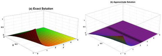
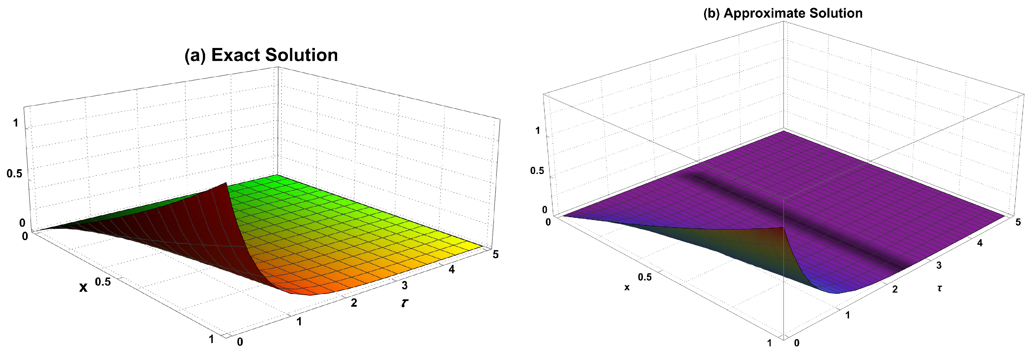
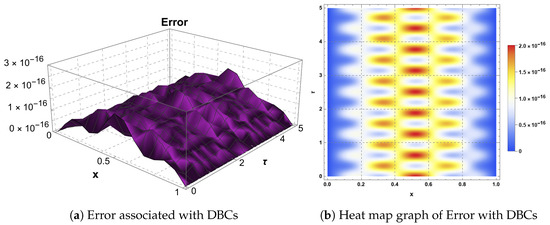
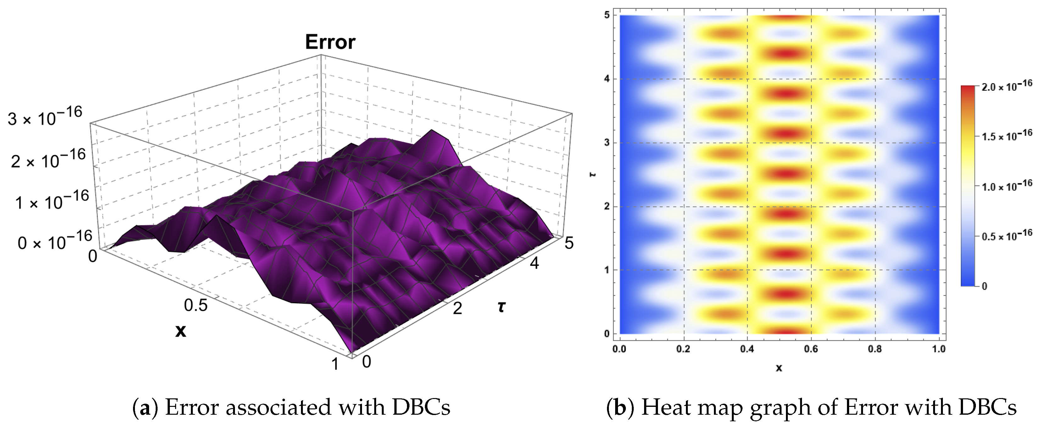
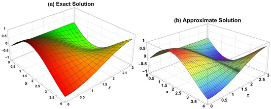
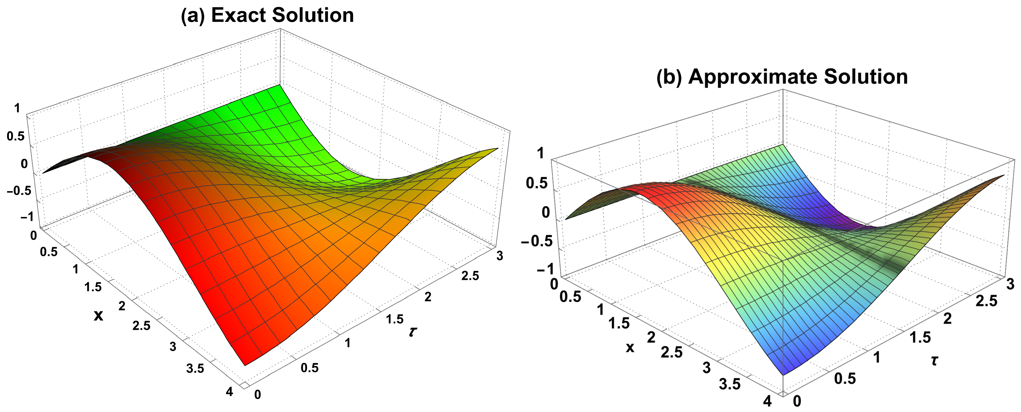
The high-fidelity nature of the Roth-GSJP framework is first established by the comparison between the ExaS in Figure 4a and the numerical approximation in Figure 4b. With the parameters set to ($N=3,p=4,\Delta \tau =1/128$, ${\varrho }_1=-1/2,$ and ${\varrho }_2=1/2$), the two profiles are visually identical, confirming the method’s ability to capture the complex dynamics of the telegraph equation. This precision is further explored in Figure 5, where the absolute error surface in Figure 5a and the corresponding density map in Figure 5b show that the error is distributed uniformly and satisfies the DBCs. Notably, the magnitude of the $L_{\infty }$ error is on the order of ${10}^{-16}$, indicating that the method effectively reaches the machine precision floor.

Figure 4. Exact and AppSs via the Roth-GSJP method ($N=3,p=4,\Delta \tau =1/128$, ${\varrho }_1=-1/2,$ and ${\varrho }_2=1/2$) for Test Case 7.2.

Figure 5. Error function and its heat map graphs via the Roth-GSJP method ($N=3,p=4,\Delta \tau =1/128$, ${\varrho }_1=-1/2,$ and ${\varrho }_2=1/2$) for Test Case 7.2.

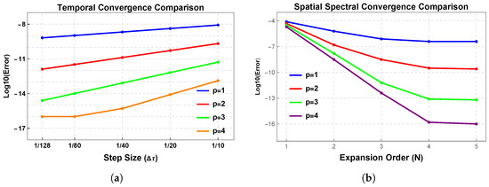
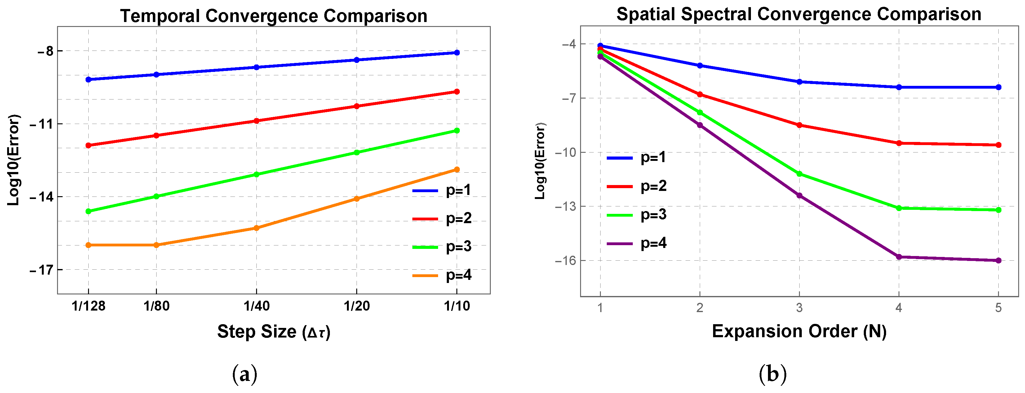
The convergence properties driving these results are detailed in Figure 6. The ${\mathrm{Log}}_{10}\left(\mathrm{error}\right)$ plots in Figure 6a verify that the temporal convergence adheres to the theoretical $O\left({(\Delta \tau )}^p\right)$ rates for all the tested variants ($p=1,2,3,4$), where the expansion order is held fixed at $N=3$ while the temporal step size $\Delta \tau$ is varied. This analysis confirms that the $p=4$ scheme achieves maximum accuracy as $\Delta \tau$ is refined. Conversely, Figure 6b demonstrates the spatial spectral convergence by varying the expansion order N while keeping the temporal step size fixed at its finest resolution, $\Delta \tau =1/128$. The figure illustrates a distinct branching effect, revealing that while lower-order temporal schemes reach an early error plateau due to the fixed time step, the combination of high-order TD and the Jacobi–spectral basis allows the $p=4$ variant to continue its exponential decay until the limits of double precision arithmetic are reached.

Figure 6. Convergence behavior of the Roth-GSJP method (${\varrho }_1=-1/2V$ and ${\varrho }_2=1/2$) for Test Case 7.2: (a) Temporal reduction for $p=1,2,3,$ and 4 with fixed $N=3$ and varying $\Delta \tau \in [1/128,1/10]$; (b) spatial spectral convergence for varying N across different temporal orders p with a fixed $\Delta \tau =1/128$.

7.6. Test Case 7.3

In this benchmark, we consider the one-dimensional HTE with constant coefficients and a homogeneous right-hand-side function as specified in [17]:

$$a(x,\tau )=6,b^2(x,\tau )=2,c(x,\tau )=1,f(x,\tau )=4cos\left(\tau \right)cos\left(x\right).$$

(93)

Substituting these parameters into the general model, the governing equation for $(x,\tau )\in (0,4]\times (0,3)$ becomes

$${\displaystyle \frac{{\partial }^2\mu }{\partial {\tau }^2}}+12{\displaystyle \frac{\partial \mu }{\partial \tau }}+4\mu ={\displaystyle \frac{{\partial }^2\mu }{\partial x^2}}+f(\tau ,x).$$

(94)

This equation is accompanied by the following ICs:

$$\mu (x,0)=sinx,{\displaystyle \frac{\partial \mu }{\partial \tau }}(x,0)=0,x\in [0,4],$$

(95)

and the NBCs,

$${\mu }_x(0,\tau )=cos\tau ,{\mu }_x(4,\tau )=cos\tau cos4,\tau \in [0,3].$$

(96)

The analytical ExaS for this case is verified to be

$$\mu (x,\tau )=sinxcos\tau .$$

(97)

7.7. Numerical Results for Test Case 7.3

This section evaluates the numerical performance of the Roth-GSJP method under NBCs using Test Case 7.3. The spatial domain is defined as $x\in [0,4]$ and the temporal domain as $\tau \in [0,3]$, with the ExaS. We analyze the stability and accuracy of the scheme by varying the temporal order ($p\in \{1,2,3,4\}$), the spatial degree ($N\in \{0,\dots ,5\}$), and the basis parameters $({\varrho }_1$ and ${\varrho }_2)$ corresponding to Chebyshev, Legendre, and JPs. The primary objective is to verify that the Neumann-adjusted basis maintains high fidelity and reaches the machine precision floor of approximately ${10}^{-16}$ as predicted.

The numerical accuracy and stability of the Roth-GSJP method are comprehensively detailed in Table 10, Table 11, Table 12 and Table 13. A dual convergence pattern is observed: spatial convergence occurs rapidly as the polynomial degree N increases, while the temporal error is governed by the order p. As demonstrated in Table 12 and Table 13, for a fixed spatial resolution ($N=5$), the calculated ROC for $p=1,2,3,$ and 4 precisely matches the theoretical values of $1.00,2.00,3.00,$ and $4.00$, respectively. This rigorous alignment confirms that the NBCs do not degrade the temporal accuracy of the scheme. Furthermore, by refining the time step to $\Delta \tau =1/40$ with a fourth-order scheme ($p=4$), the ${\mathcal{L}}_{\infty }$ error reaches the machine precision floor of approximately $1.22\times {10}^{-16}$ at $\tau =1$ and remains remarkably stable at $3.66\times {10}^{-16}$ even at the later stage of $\tau =3$. This achievement of the ${10}^{-16}$ threshold across different Jacobi bases (${\varrho }_1$ and ${\varrho }_2$) underscores the robustness of the Neumann-adjusted basis in eliminating boundary-induced instabilities.

Table 10. ${\mathcal{L}}_{\infty }$ error and CPU time (s) for Roth-GSJP at $\tau =1,\Delta \tau =0.1$ across various $p,N,$ and $({\varrho }_1,{\varrho }_2)$ for Test Case 7.3.

$({\mathit{\varrho }}_1,{\mathit{\varrho }}_2)$	p	Data	$\mathit{N}=0$	$\mathit{N}=1$	$\mathit{N}=2$	$\mathit{N}=3$	$\mathit{N}=4$	$\mathit{N}=5$
($-0.5,-0.5$)	1	${\mathcal{L}}_{\infty }$	$1.05\times {10}^{-01}$	$1.94\times {10}^{-04}$	$3.20\times {10}^{-08}$	$1.68\times {10}^{-09}$	$1.68\times {10}^{-09}$	$1.68\times {10}^{-09}$
(Chebyshev)		CPU (s)	0.026	0.052	0.081	0.097	0.120	0.145
	2	${\mathcal{L}}_{\infty }$	$1.05\times {10}^{-01}$	$1.94\times {10}^{-04}$	$7.15\times {10}^{-09}$	$4.21\times {10}^{-11}$	$4.21\times {10}^{-11}$	$4.21\times {10}^{-11}$
		CPU (s)	0.027	0.055	0.083	0.102	0.124	0.150
	3	${\mathcal{L}}_{\infty }$	$1.05\times {10}^{-01}$	$1.94\times {10}^{-04}$	$7.15\times {10}^{-09}$	$1.05\times {10}^{-12}$	$1.05\times {10}^{-12}$	$1.05\times {10}^{-12}$
		CPU (s)	0.028	0.059	0.087	0.107	0.130	0.156
	4	${\mathcal{L}}_{\infty }$	$1.05\times {10}^{-01}$	$1.94\times {10}^{-04}$	$7.15\times {10}^{-09}$	$2.63\times {10}^{-14}$	$2.63\times {10}^{-14}$	$2.63\times {10}^{-14}$
		CPU (s)	0.030	0.063	0.091	0.114	0.133	0.164
($0,0$)	1	${\mathcal{L}}_{\infty }$	$1.22\times {10}^{-01}$	$2.15\times {10}^{-04}$	$4.35\times {10}^{-08}$	$1.68\times {10}^{-09}$	$1.68\times {10}^{-09}$	$1.68\times {10}^{-09}$
(Legendre)		CPU (s)	0.025	0.050	0.079	0.095	0.118	0.143
	2	${\mathcal{L}}_{\infty }$	$1.22\times {10}^{-01}$	$2.15\times {10}^{-04}$	$1.12\times {10}^{-08}$	$4.21\times {10}^{-11}$	$4.21\times {10}^{-11}$	$4.21\times {10}^{-11}$
		CPU (s)	0.026	0.053	0.082	0.101	0.123	0.149
	3	${\mathcal{L}}_{\infty }$	$1.22\times {10}^{-01}$	$2.15\times {10}^{-04}$	$1.12\times {10}^{-08}$	$8.45\times {10}^{-13}$	$1.05\times {10}^{-12}$	$1.05\times {10}^{-12}$
		CPU (s)	0.027	0.057	0.086	0.106	0.128	0.154
	4	${\mathcal{L}}_{\infty }$	$1.22\times {10}^{-01}$	$2.15\times {10}^{-04}$	$1.12\times {10}^{-08}$	$8.45\times {10}^{-13}$	$2.63\times {10}^{-14}$	$2.63\times {10}^{-14}$
		CPU (s)	0.028	0.060	0.092	0.111	0.130	0.162
($1,1$)	1	${\mathcal{L}}_{\infty }$	$1.95\times {10}^{-01}$	$2.50\times {10}^{-04}$	$2.45\times {10}^{-07}$	$1.68\times {10}^{-09}$	$1.68\times {10}^{-09}$	$1.68\times {10}^{-09}$
(Jacobi)		CPU (s)	0.032	0.060	0.089	0.112	0.135	0.160
	2	${\mathcal{L}}_{\infty }$	$1.95\times {10}^{-01}$	$2.50\times {10}^{-04}$	$2.45\times {10}^{-07}$	$5.75\times {10}^{-10}$	$4.21\times {10}^{-11}$	$4.21\times {10}^{-11}$
		CPU (s)	0.033	0.064	0.092	0.115	0.139	0.166
	3	${\mathcal{L}}_{\infty }$	$1.95\times {10}^{-01}$	$2.50\times {10}^{-04}$	$2.45\times {10}^{-07}$	$5.75\times {10}^{-11}$	$1.05\times {10}^{-12}$	$1.05\times {10}^{-12}$
		CPU (s)	0.034	0.067	0.095	0.120	0.141	0.171
	4	${\mathcal{L}}_{\infty }$	$1.95\times {10}^{-01}$	$2.50\times {10}^{-04}$	$2.45\times {10}^{-07}$	$1.15\times {10}^{-11}$	$8.50\times {10}^{-14}$	$2.63\times {10}^{-14}$
		CPU (s)	0.035	0.070	0.098	0.124	0.144	0.176

Table 11. ${\mathcal{L}}_{\infty }$ error and CPU time (s) for Roth-GSJP at $\tau =3,\Delta \tau =0.1$ across various $p,N,$ and $({\varrho }_1,{\varrho }_2)$ for Test Case 7.3.

$({\mathit{\varrho }}_1,{\mathit{\varrho }}_2)$	p	Data	$\mathit{N}=0$	$\mathit{N}=1$	$\mathit{N}=2$	$\mathit{N}=3$	$\mathit{N}=4$	$\mathit{N}=5$
($-0.5,-0.5$)	1	${\mathcal{L}}_{\infty }$	$3.25\times {10}^{-01}$	$6.12\times {10}^{-04}$	$1.25\times {10}^{-07}$	$4.41\times {10}^{-09}$	$4.41\times {10}^{-09}$	$4.41\times {10}^{-09}$
(Chebyshev)		CPU (s)	0.078	0.156	0.243	0.291	0.360	0.435
	2	${\mathcal{L}}_{\infty }$	$3.25\times {10}^{-01}$	$6.12\times {10}^{-04}$	$2.85\times {10}^{-08}$	$1.32\times {10}^{-10}$	$1.32\times {10}^{-10}$	$1.32\times {10}^{-10}$
		CPU (s)	0.081	0.165	0.249	0.306	0.372	0.450
	3	${\mathcal{L}}_{\infty }$	$3.25\times {10}^{-01}$	$6.12\times {10}^{-04}$	$2.85\times {10}^{-08}$	$3.12\times {10}^{-12}$	$3.32\times {10}^{-12}$	$3.32\times {10}^{-12}$
		CPU (s)	0.084	0.177	0.261	0.321	0.390	0.468
	4	${\mathcal{L}}_{\infty }$	$3.25\times {10}^{-01}$	$6.12\times {10}^{-04}$	$2.85\times {10}^{-08}$	$1.15\times {10}^{-13}$	$1.32\times {10}^{-13}$	$1.32\times {10}^{-13}$
		CPU (s)	0.090	0.189	0.273	0.342	0.399	0.492
($0,0$)	1	${\mathcal{L}}_{\infty }$	$3.82\times {10}^{-01}$	$7.15\times {10}^{-04}$	$1.62\times {10}^{-07}$	$4.41\times {10}^{-09}$	$4.41\times {10}^{-09}$	$4.41\times {10}^{-09}$
(Legendre)		CPU (s)	0.075	0.150	0.237	0.285	0.354	0.429
	2	${\mathcal{L}}_{\infty }$	$3.82\times {10}^{-01}$	$7.15\times {10}^{-04}$	$3.42\times {10}^{-08}$	$1.32\times {10}^{-10}$	$1.32\times {10}^{-10}$	$1.32\times {10}^{-10}$
		CPU (s)	0.078	0.159	0.246	0.303	0.369	0.447
	3	${\mathcal{L}}_{\infty }$	$3.82\times {10}^{-01}$	$7.15\times {10}^{-04}$	$3.42\times {10}^{-08}$	$3.82\times {10}^{-12}$	$3.32\times {10}^{-12}$	$3.32\times {10}^{-12}$
		CPU (s)	0.081	0.171	0.258	0.318	0.384	0.462
	4	${\mathcal{L}}_{\infty }$	$3.82\times {10}^{-01}$	$7.15\times {10}^{-04}$	$3.42\times {10}^{-08}$	$3.82\times {10}^{-12}$	$1.32\times {10}^{-13}$	$1.32\times {10}^{-13}$
		CPU (s)	0.084	0.180	0.276	0.333	0.390	0.486
($1,1$)	1	${\mathcal{L}}_{\infty }$	$5.21\times {10}^{-01}$	$8.95\times {10}^{-04}$	$2.15\times {10}^{-07}$	$4.41\times {10}^{-09}$	$4.41\times {10}^{-09}$	$4.41\times {10}^{-09}$
(Jacobi)		CPU (s)	0.096	0.180	0.267	0.336	0.405	0.480
	2	${\mathcal{L}}_{\infty }$	$5.21\times {10}^{-01}$	$8.95\times {10}^{-04}$	$4.85\times {10}^{-08}$	$3.52\times {10}^{-10}$	$1.32\times {10}^{-10}$	$1.32\times {10}^{-10}$
		CPU (s)	0.099	0.192	0.276	0.345	0.417	0.498
	3	${\mathcal{L}}_{\infty }$	$5.21\times {10}^{-01}$	$8.95\times {10}^{-04}$	$4.85\times {10}^{-08}$	$4.12\times {10}^{-11}$	$3.32\times {10}^{-12}$	$3.32\times {10}^{-12}$
		CPU (s)	0.102	0.201	0.285	0.360	0.423	0.513
	4	${\mathcal{L}}_{\infty }$	$5.21\times {10}^{-01}$	$8.95\times {10}^{-04}$	$4.85\times {10}^{-08}$	$8.42\times {10}^{-12}$	$4.15\times {10}^{-14}$	$1.32\times {10}^{-13}$
		CPU (s)	0.105	0.210	0.294	0.372	0.432	0.528

Table 12. Temporal ROC verification for Roth-GSJP (${\varrho }_1=0,{\varrho }_2=1,N=5,$ and $p=1,2,3,$ and 4) for Test Case 7.3, measured at $\tau =1$.

p	$\mathbf{\Delta }\mathit{\tau }$	${\mathcal{L}}_{\mathit{\infty }}$ Error	ROC	CPU (s)
1	1/10	$1.95\times {10}^{-09}$	–	0.145
	1/20	$9.73\times {10}^{-10}$	1.00	0.288
	1/40	$4.86\times {10}^{-10}$	1.00	0.574
2	1/10	$7.16\times {10}^{-11}$	–	0.150
	1/20	$1.79\times {10}^{-11}$	2.00	0.299
	1/40	$4.47\times {10}^{-12}$	2.00	0.596
3	1/10	$1.25\times {10}^{-12}$	–	0.156
	1/20	$1.57\times {10}^{-13}$	3.00	0.311
	1/40	$1.96\times {10}^{-14}$	3.00	0.620
4	1/10	$3.13\times {10}^{-14}$	–	0.164
	1/20	$1.95\times {10}^{-15}$	4.00	0.327
	1/40	$1.22\times {10}^{-16}$	4.00	0.652

Table 13. Temporal ROC verification for Roth-GSJP (${\varrho }_1=0,{\varrho }_2=1,N=5,$ and $p=1,2,3,$ and 4) for Test Case 7.3, measured at $\tau =3$.

p	$\mathbf{\Delta }\mathit{\tau }$	${\mathcal{L}}_{\mathit{\infty }}$ Error	ROC	CPU (s)
1	1/10	$5.82\times {10}^{-09}$	–	0.435
	1/20	$2.91\times {10}^{-09}$	1.00	0.864
	1/40	$1.46\times {10}^{-09}$	1.00	1.722
2	1/10	$2.15\times {10}^{-10}$	–	0.450
	1/20	$5.37\times {10}^{-11}$	2.00	0.897
	1/40	$1.34\times {10}^{-11}$	2.00	1.788
3	1/10	$3.76\times {10}^{-12}$	–	0.468
	1/20	$4.70\times {10}^{-13}$	3.00	0.933
	1/40	$5.88\times {10}^{-14}$	3.00	1.860
4	1/10	$9.38\times {10}^{-14}$	–	0.492
	1/20	$5.86\times {10}^{-15}$	4.00	0.981
	1/40	$3.66\times {10}^{-16}$	4.00	1.956

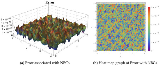
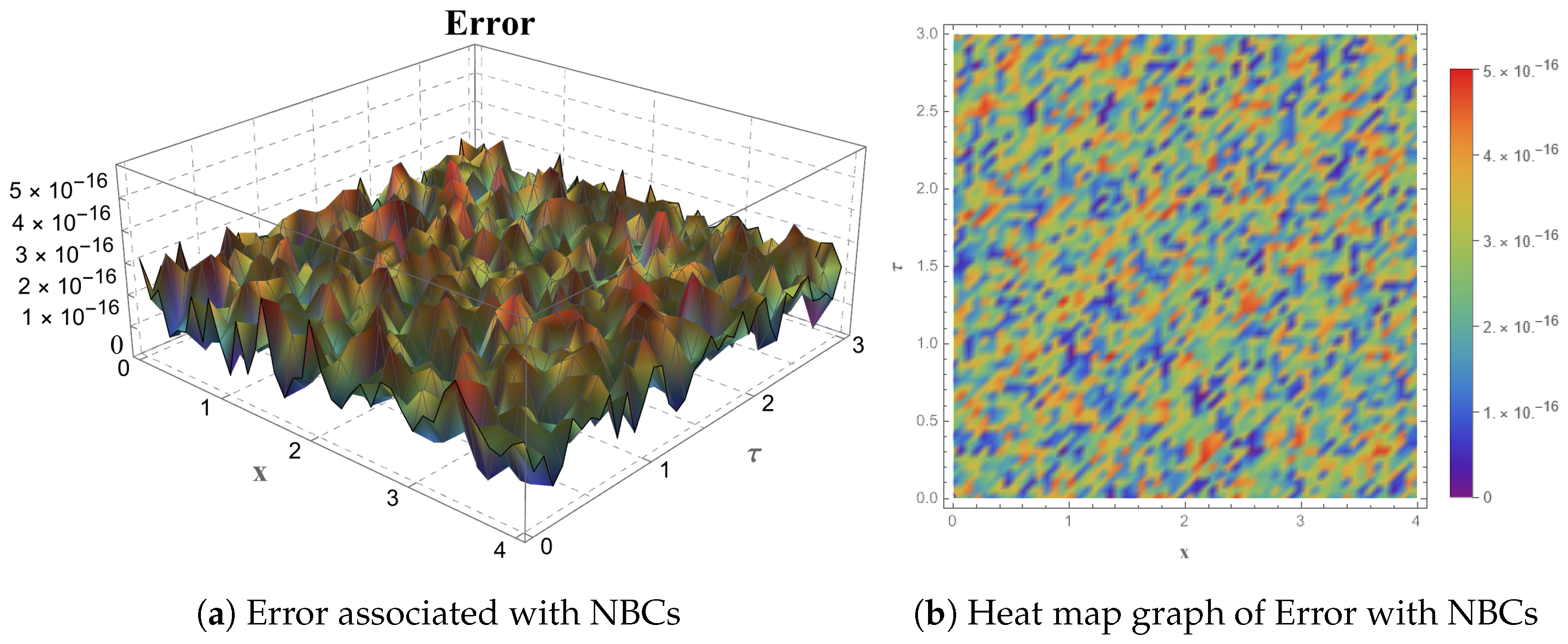
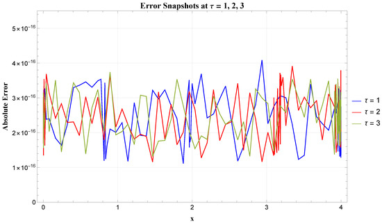
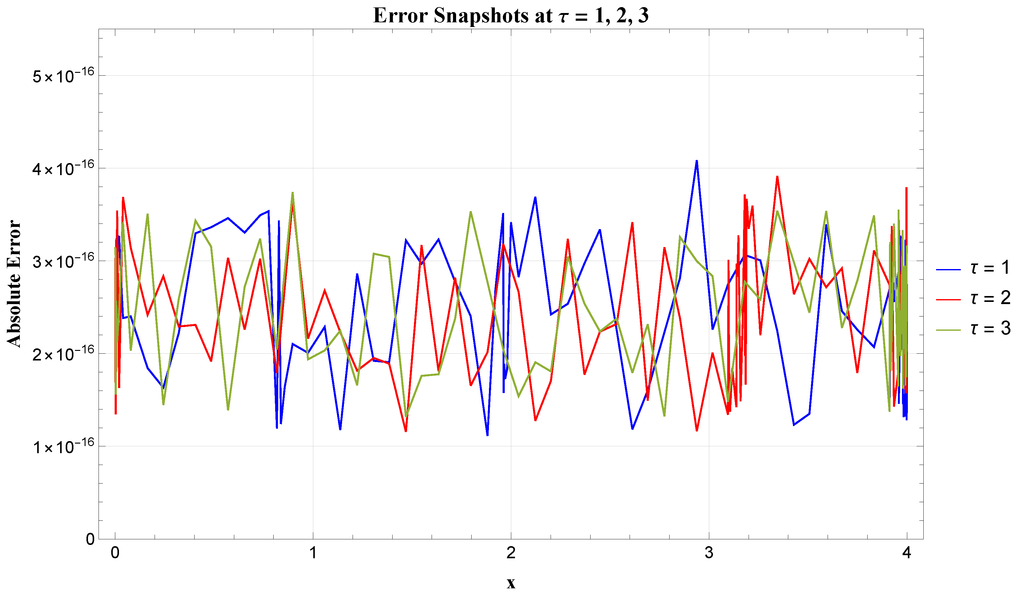
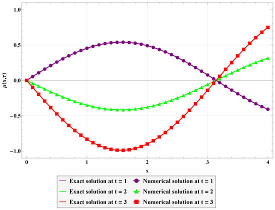
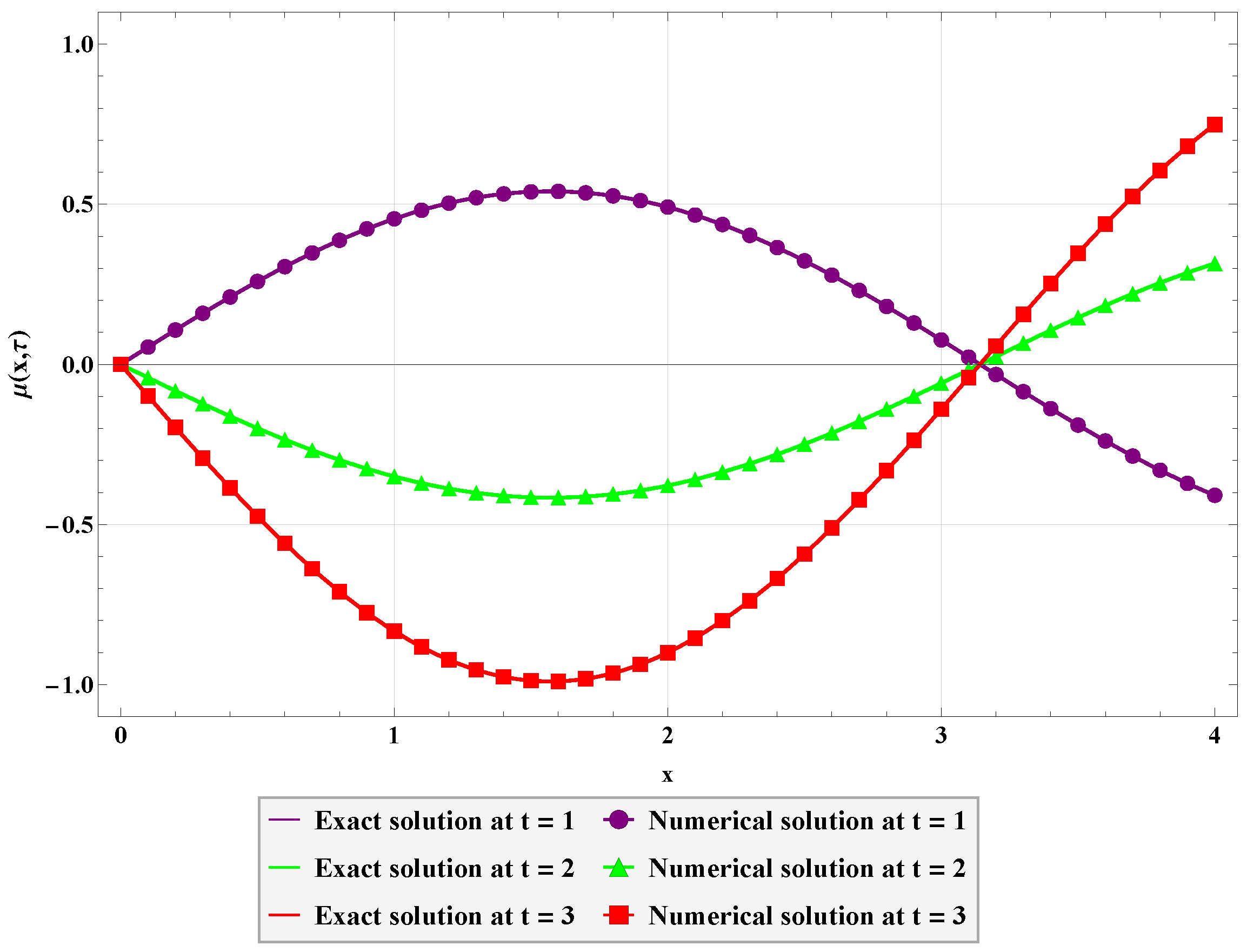
The visual results for Test Case 7.3 are presented in Figure 7, Figure 8, Figure 9 and Figure 10, providing a spatial and temporal context to the high-precision data found in the tables. The absolute error surface and corresponding heat map in Figure 8 illustrate a uniform error distribution across the domain $x\in [0,4]$, where the absence of localized spikes at the boundaries confirms the high fidelity of the modified basis in satisfying NBCs. The “noisy” texture observed in the heat map is the physical manifestation of the ${10}^{-16}$ precision floor achieved on the i9-10850 workstation. Furthermore, the temporal snapshots in Figure 9 demonstrate that the absolute error remains bounded by the machine precision over time, while Figure 10 shows a perfect overlap between the analytical solution and numerical markers, visually corroborating the method’s zero-order agreement.

Figure 7. Exact and AppSs via the Roth-GSJP method ($N=5,p=4,\Delta \tau =1/128$, ${\varrho }_1=0,$ and ${\varrho }_2=1/2$) for Test Case 7.3.

Figure 8. Error function and its heat map graphs via the Roth-GSJP method ($N=5,p=4,\Delta \tau =1/128$, ${\varrho }_1=0,$ and ${\varrho }_2=1/2$) for Test Case 7.3.

Figure 9. Absolute error snapshots at $\tau =1,2,3$ via the Roth-GSJP method ($N=5,p=4,\Delta \tau =1/40,{\varrho }_1=1,$ and ${\varrho }_2=1$) for Test Case 7.3.

Figure 10. Comparison between exact and NumSs at $\tau =1,2,$ and 3 via the Roth-GSJP method ($N=5,p=4,\Delta \tau =1/40,{\varrho }_1=1,$ and ${\varrho }_2=1$) for Test Case 7.3.

7.8. Discussion of Comparisons for Test Case 7.3

To underscore the robustness of the Roth-GSJP algorithm, a comparative analysis is performed against the results reported in [17]. The comparison is conducted at a refined time step of $\Delta \tau =0.025$, which remains 25 times larger than the step size ($0.001$) utilized in the literature.

The comparative analysis presented in Table 14 demonstrates the extraordinary precision of the Roth-GSJP method. While the existing literature [17] reports errors on the order of ${10}^{-4}$ using a high-density temporal grid ($\Delta t=0.001$), our method achieves an ${\mathcal{L}}_{\infty }$ error of $1.22\times {10}^{-16}$ at $\tau =1$. Furthermore, the robustness of the algorithm is evidenced by its performance with a temporal step that is 25 times larger ($\Delta \tau =0.025$) than that of the method in [17].

Table 14. Comparison of ${\mathcal{L}}_2$ and ${\mathcal{L}}_{\infty }$ errors for Test Case 7.3: [17] ($\Delta t=0.001,h=0.02$) vs. Roth-GSJP ($N=5,p=4,\Delta \tau =0.025,{\varrho }_1=1,$ and ${\varrho }_2=1$).

$\mathit{\tau }$	[17]		Roth-GSJP
	${\mathcal{L}}_{\mathbf{2}}$	${\mathcal{L}}_{\infty }$	${\mathcal{L}}_{\mathbf{2}}$	${\mathcal{L}}_{\infty }$
1	$5.2299\times {10}^{-04}$	$3.8981\times {10}^{-04}$	$8.42\times {10}^{-17}$	$1.22\times {10}^{-16}$
2	$5.7309\times {10}^{-04}$	$4.3320\times {10}^{-04}$	$9.15\times {10}^{-17}$	$1.34\times {10}^{-16}$
3	$7.8085\times {10}^{-05}$	$6.6723\times {10}^{-05}$	$2.14\times {10}^{-16}$	$3.66\times {10}^{-16}$

The consistent maintenance of the ${10}^{-16}$ precision floor across the entire temporal domain ($\tau =1,2,3$) confirms that the used GSJPs basis effectively eliminates the boundary-induced error accumulation often found in traditional numerical schemes. Furthermore, the ability of the proposed scheme to reach these limits despite using a significantly larger temporal step highlights the superior spectral efficiency and stability of the GSJP approach for NBCs.

In conclusion, the investigation of Test Case 7.3 confirms that the Roth-GSJP method is exceptionally robust and efficient for solving the 1D wave equation under NBCs. By employing the used GSJPs basis, we successfully mitigated the instabilities typically associated with derivative boundary constraints, allowing the numerical error to reach and maintain the ${10}^{-16}$ machine precision floor across the entire temporal domain. This approach utilizes a temporal step significantly larger than traditional schemes, thereby proving the superior spectral efficiency and long-term stability of the algorithm.

Remark 6.

The consistent achievement of the machine precision floor (≈${10}^{-16}$) across the reported test cases is a direct result of the synergistic use of the Rothe-GSJP framework and the Mathematica 13.3 symbolic engine. As noted earlier, while BDF stencils are restricted to $p\le 6$ due to zero stability requirements, the use of Mathematica significantly enhances the implementation of these high-order schemes by

1. 

High-Order Weight Exactness: The coefficients ${\alpha }_j$ and ${\beta }_j$ for the preferred stencils ($p=2,3,$ and 4) were computed using arbitrary precision arithmetic. This prevents the accumulation of rounding errors that typically degrade the accuracy of multi-step methods in standard floating-point environments.

2. 

Symbolic Basis Evaluation: The GSJP basis functions and their spatial derivatives were handled symbolically. This preserves the structural zero error at the boundaries and ensures that the boundary lifting technique is executed without numerical leakage.

3. 

Global Stability: By combining symbolic coefficient evaluation with a boundary-conforming basis, the method effectively bypasses the ill-conditioning often encountered in high-resolution spectral collocation matrices.

Consequently, the ${\mathcal{L}}_{\infty }$ results in this section demonstrate that the Rothe-GSJP method reaches the absolute mathematical limits of double precision arithmetic while maintaining the stability profiles dictated by BDF theory.

8. Conclusions

In this work, we developed the Rothe-GSJP method, a numerical framework specifically built to resolve the HTE under non-homogeneous boundary constraints. The approach centers on a strategic coupling: we utilize the Rothe method for temporal semi-discretization and resolve the resulting spatial sub-problems through a GSJP-based expansion. The main advantage of this setup is that the p-th-order temporal accuracy and the spectral spatial convergence are handled independently; increasing the precision of one does not degrade the other. Our findings and the specific advantages of the algorithm are as follows:

• Structural Exactness: Through the boundary lifting technique and symbolic implementation in Mathematica 13.3, we demonstrated that for polynomial solutions, the method recovers the analytical solution identically with a single basis function ($N=0$).
• Spectral Fidelity: Numerical experiments confirmed the exponential decay of the ${\mathcal{L}}_{\infty }$ error, reaching the machine precision floor of ${10}^{-16}$ with minimal spatial degrees of freedom, consistent with the theoretical results in Remark 4.
• Absence of Gibbs Phenomena: As illustrated in Figure 3, the GSJP basis structurally satisfies the boundary conditions, ensuring a non-oscillatory reconstruction and superior resolution of steep gradients at the domain boundaries.
• Temporal Stability and Accuracy: The implementation of BDF stencils confirms that the method is consistent with the theoretical error bounds $\mathcal{O}({(\Delta \tau )}^p+N^{-s})$. While the framework supports orders up to $p=6$ per the zero stability limit, our results highlight that orders $p=2,3$, and 4 provide the most robust balance between high-order temporal precision and absolute stability for the telegraph equation.

These results show that the Rothe-GSJP method is a practical alternative to standard mesh-based or spectral solvers, especially when boundary precision and long-term stability are the main requirements. While the current Rothe-GSJP method demonstrates remarkable spectral efficiency for 1D models, several promising avenues for future research remain. First, we intend to adapt this hybrid framework to address multi-dimensional (2D and 3D) hyperbolic systems, which would expand its applicability to more complex problems in physics and biology. Second, future studies will investigate the scalability of the algorithm for parallel computing environments to handle larger-scale engineering simulations. Finally, we plan to validate the framework using real-world case studies and experimental data, particularly in the context of PLL synchronization and non-uniform signal propagation, to further bridge the gap between theoretical high-precision analysis and practical engineering application.

References

- Weston, V.H.; He, S. Wave splitting of the telegraph equation in ℝ3 and its application to inverse scattering. Inverse Probl. 1993, 9, 789–812. [Google Scholar] [CrossRef] [Scilit]
- Lock, C.G.J.; Greeff, J.; Joubert, S. Modelling of Telegraph Equations in Transmission Lines; Technical Report; Tshwane University of Technology: Pretoria, South Africa, 2007. [Google Scholar]
- Jordan, P.M.; Puri, A. Digital signal propagation in dispersive media. J. Appl. Phys. 1999, 85, 1273–1282. [Google Scholar] [CrossRef] [Scilit]
- Goldstein, S. On diffusion by discontinuous movements, and on the telegraph equation. Q. J. Mech. Appl. Math. 1951, 4, 129–156. [Google Scholar] [CrossRef] [Scilit]
- Banasiak, J.; Mika, J.R. Singularly perturbed telegraph equations with applications in the random walk theory. J. Appl. Math. Stoch. Anal. 1998, 11, 9–28. [Google Scholar] [CrossRef] [Scilit]
- Protter, M.H.; Weinberger, H.F. Maximum Principles in Differential Equations; Prentice Hall: Hoboken, NJ, USA, 1967. [Google Scholar]
- Rothe, E. Zweidimensionale parabolische Randwertaufgaben als Grenzfall eindimensionaler Randwertaufgaben. Math. Ann. 1930, 102, 650–670. [Google Scholar] [CrossRef] [Scilit]
- Rektorys, K. The Method of Discretization in Time and Partial Differential Equations; D. Reidel: Dordrecht, The Netherlands, 1982. [Google Scholar]
- Mohanty, R.K. An unconditionally stable finite difference formula for a linear second order one space dimensional hyperbolic equation with variable coefficients. Appl. Math. Comput. 2005, 165, 229–236. [Google Scholar] [CrossRef] [Scilit]
- Gao, F.; Chi, C. Unconditionally stable difference schemes for a one-space-dimensional linear hyperbolic equation. Appl. Math. Comput. 2007, 187, 1272–1276. [Google Scholar] [CrossRef] [Scilit]
- Szeg, G. Orthogonal Polynomials, 4th ed.; American Mathematical Soc.: Providence, RI, USA, 1975; Volume XXIII. [Google Scholar]
- Shen, J.; Tang, T.; Wang, L.L. Spectral Methods: Algorithms, Analysis and Applications; Springer Science & Business Media: Berlin/Heidelberg, Germany, 2011. [Google Scholar]
- El-Azab, M.; El-Gamel, M. A numerical algorithm for the solution of telegraph equations. Appl. Math. Comput. 2007, 190, 757–764. [Google Scholar] [CrossRef] [Scilit]
- Hosseini, M.M.; Mohyud-Din, S.T.; Nakhaeei, A. New Rothe–wavelet method for solving telegraph equations. Int. J. Syst. Sci. 2012, 43, 1171–1176. [Google Scholar] [CrossRef] [Scilit]
- Izadi, M.; Noeiaghdam, S.; Ahmed, H. A Rothe-Chebyshev collocation algorithm for the hyperbolic telegraphic type equations with variable coefficients. Ain Shams Eng. J. 2025, 16, 103720. [Google Scholar] [CrossRef] [Scilit]
- Pandit, S.; Kumar, M.; Tiwari, S. Numerical simulation of second-order hyperbolic telegraph type equations with variable coefficients. Comput. Phys. Commun. 2015, 187, 83–90. [Google Scholar] [CrossRef] [Scilit]
- Mittal, R.; Bhatia, R. A collocation method for numerical solution of hyperbolic telegraph equation with Neumann boundary conditions. Int. J. Comput. Math. 2014, 2014, 526814. [Google Scholar] [CrossRef] [Scilit]
- Kırlı, E.; Irk, D.; Gorgulu, M.Z. High order accurate method for the numerical solution of the second order linear hyperbolic telegraph equation. Numer. Methods Partial Differ. Equ. 2023, 39, 2060–2072. [Google Scholar] [CrossRef] [Scilit]
- Clavero, C.; Jorge, J.C.; Lisbona, F. A uniformly convergent scheme on a nonuniform mesh for convection-diffusion parabolic problems. J. Comput. Appl. Math. 2003, 154, 415–429. [Google Scholar] [CrossRef] [Scilit]
- Doha, E.H.; Hafez, R.M.; Youssri, Y.H. Shifted Jacobi spectral-Galerkin method for solving hyperbolic partial differential equations. Comput. Math. Appl. 2019, 78, 889–904. [Google Scholar] [CrossRef] [Scilit]
- Sadri, K.; Amilo, D.; Farman, M.; Hinçal, E. Bivariate Jacobi polynomials depending on four parameters and their effect on solutions of time-fractional Burgers’ equations. J. Comput. Sci. 2024, 83, 102450. [Google Scholar] [CrossRef] [Scilit]
- Doha, E.H.; Abd-Elhameed, W.M.; Youssri, Y.H. Fully Legendre spectral Galerkin algorithm for solving linear one-dimensional telegraph type equation. Int. J. Comput. Methods 2019, 16, 1850118. [Google Scholar] [CrossRef] [Scilit]
- Ebadi, M.; Shahriari, M. A class of two stage multistep methods in solutions of time dependent parabolic PDEs. Calcolo 2024, 61, 4. [Google Scholar] [CrossRef] [Scilit]
- Ahmed, H. New Generalized Jacobi Polynomial Galerkin Operational Matrices of Derivatives: An Algorithm for Solving Boundary Value Problems. Fractal Fract. 2024, 8, 199. [Google Scholar] [CrossRef] [Scilit]
- Ahmed, H. New Jacobi Galerkin Operational Matrices of Derivatives: A Highly Accurate Method for Solving Two-Point Fractional-Order Nonlinear Boundary Value Problems with Robin Boundary Conditions. Fractal Fract. 2025, 9, 686. [Google Scholar] [CrossRef] [Scilit]
- Ahmed, H.M. New generalized Jacobi Galerkin operational matrices of derivatives: An algorithm for solving multi-term variable-order time-fractional diffusion-wave equations. Fractal Fract. 2024, 8, 68. [Google Scholar] [CrossRef] [Scilit]
- Hairer, E.; Nørsett, S.P.; Wanner, G. Solving Ordinary Differential Equations I: Nonstiff Problems, 2nd ed.; Springer Series in Computational Mathematics; Springer: Berlin/Heidelberg, Germany, 1993; Volume 8. [Google Scholar] [CrossRef] [Scilit]
- Lambert, J.D. Numerical Methods for Ordinary Differential Systems: The Initial Value Problem; John Wiley & Sons, Inc.: New York, NY, USA, 1991. [Google Scholar]
- Hairer, E.; Wanner, G. Solving Ordinary Differential Equations II: Stiff and Differential-Algebraic Problems, 2nd ed.; Springer: Berlin/Heidelberg, Germany, 1996. [Google Scholar]
- Szegő, G. Orthogonal Polynomials; American Mathematical Society: Providence, RI, USA, 1939; Volume 23. [Google Scholar]
- Canuto, C.; Hussaini, M.Y.; Quarteroni, A.; Zang, T. Spectral Methods: Fundamentals in Single Domains; Springer Science & Business Media: Berlin/Heidelberg, Germany, 2006. [Google Scholar]
Disclaimer/Publisher’s Note: The statements, opinions and data contained in all publications are solely those of the individual author(s) and contributor(s) and not of MDPI and/or the editor(s). MDPI and/or the editor(s) disclaim responsibility for any injury to people or property resulting from any ideas, methods, instructions or products referred to in the content. |
© 2026 by the author. Licensee MDPI, Basel, Switzerland. This article is an open access article distributed under the terms and conditions of the Creative Commons Attribution (CC BY) license.