Hierarchically Coupled Biochemical Switches for Stem Cell Differentiation

Abstract

In multicellular organisms, the development of diverse cell types relies on stem cell differentiation through a hierarchy of fate decisions. Pluripotent stem cells first give rise to multipotent progenitors, which then undergo successive fate decisions to generate specialized cells within their respective lineages. Waddington used the metaphor of a marble rolling down a hill through hierarchically branching valleys that represent the various states of cell differentiation, with the final valleys at the bottom symbolizing the specialized cells. Mathematically, specialized cells are seen as stable attractors in a complex dynamical system that displays multistability. However, this framework does not necessarily describe the hierarchical branching of stem cell differentiation. In a recent study, we addressed this issue by assuming that each gene regulatory network (GRN) consists of hierarchically coupled gene subnetworks (modules) that are self-regulated due to epigenetic factors. Each module was modeled using the normal form of relevant bifurcations. Overall, this approach captures both multistability and hierarchical branching in differentiation. Here, the normal forms of bifurcations are replaced by realistic biochemical switches. Theoretical analysis and numerical simulations demonstrated that hierarchically coupled biochemical switches can depict the three fundamental aspects of Waddington’s epigenetic landscape: (a) differentiation trajectories exhibit hierarchical branching, (b) attractors are robust to perturbations (homeorhesis), and (c) the proportions of specialized cells are preserved. It was further shown that appropriate external interventions can induce either probabilistic cellular reprogramming or highly predictable reprogramming outcomes. The incorporation of biochemical switches, rather than purely abstract normal forms, can contribute to more biologically grounded mathematical models of stem cell differentiation. This work also highlights the importance of normal forms for qualitatively understanding cell state dynamics and for building realistic modular GRNs.

1. Introduction

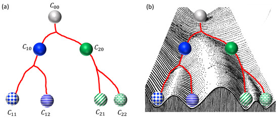
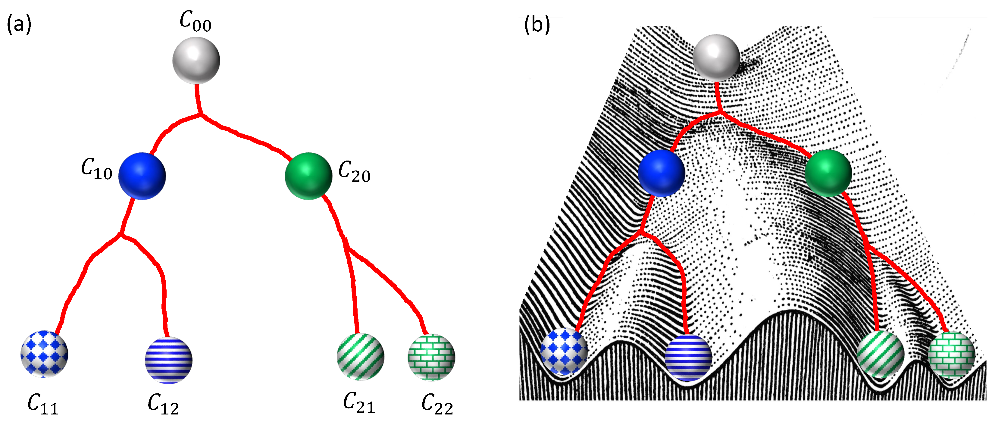
Stem cell differentiation is a hierarchically branched mechanism that gives rise to all the necessary cell types in a multicellular organism [1,2]. A schematic representation of this process is shown in Figure 1a. It begins with a stem cell undergoing an initial fate decision that produces two progenitor states. These progenitors retain limited developmental potential and can further differentiate along their own distinct lineages to produce specialized cell types. This simple example of stem cell differentiation was metaphorically described by Waddington as a marble rolling down a hill consisting of various valleys that branch sequentially (see Figure 1b) [3]. Each valley corresponds to a cell state, and each branching point to a fate decision event. Mathematically, this metaphor represents the potential function of a dynamical system that describes the stem cell’s gene regulatory network (GRN). In this representation, each valley corresponds to a stable equilibrium solution (attractor), and each decision-making event corresponds to a bifurcation point. The ratio of the produced cells should depend on the detailed structure of the potential function.

Figure 1. (a) Schematic representation of stem cell differentiation. Initially, the stem cell $C_{00}$ differentiates into two progenitor cells $C_{10}$ and $C_{20}$, which subsequently produce four different cells $C_{11}$, $C_{12}$, $C_{21}$, and $C_{22}$. (b) Waddington’s epigenetic landscape (adapted from [3]).

In the theory of dynamical systems, GRNs are commonly modeled as systems of differential equations, where each equation represents the expression levels of genes or the concentrations of associated proteins [1,2]. To simplify the mathematical analysis, such models typically consider the regulatory interactions only among the most dominant genes and proteins. Within this framework, different equilibrium points indicate the overexpression or suppression of a given gene, reflecting the existence of specific cell types. In practice, such systems often exhibit bistability or tristability. From a mathematical perspective, crossing a bifurcation point corresponds to the emergence of new equilibrium states, which, in models of cell differentiation, are interpreted as the formation of new cell types. While these dynamical systems have successfully described cellular transitions and biochemical switches, their applicability in modeling the overall differentiation process of stem cells is limited. The main challenge is that these models do not typically capture the hierarchically branched evolution of the cell, which requires autonomous navigation through multiple bifurcation points.

This challenge has been addressed in two recent studies [4,5]. In the first work [4], the authors modeled the GRN of a stem cell as a hierarchy of coupled gene subnetworks (modules). This idea is biologically well motivated, as many complex biological systems, including GRNs, exhibit a pronounced modular organization [6,7,8,9,10]. In particular, Foster et al. [4] modeled each module as a tristable dynamical system capable of mediating discrete fate decisions. One stable state corresponds to an inactive configuration, while the other two represent different functional outcomes. Initially, although all modules are in the inactive state, stochastic fluctuations induce spontaneous symmetry breaking in the first module. This initial fate decision subsequently drives the rest of the modules through their own bifurcation points. Ultimately, all modules relax into stable equilibrium states whose collective behavior determines the differentiated cell type. In the second study [5], Matsushita and Kaneko introduced a dynamical framework capable of reproducing essential features of Waddington’s epigenetic landscape. Each gene of the GRN is modeled by a differential equation with bistable on/off states and is regulated by auxiliary dynamical variables representing epigenetic modifications. The coupled system exhibits hierarchical branching, robustness to perturbations, and convergence to characteristic ratios of differentiated cell types.

In a recent study [11], we combine these two works to introduce an autonomous dynamical systems framework that captures the fundamental properties of the epigenetic landscape. The model combines the modular organization of GRNs with parameter regulation mediated by epigenetic factors. The GRN is represented as a hierarchy of interacting subnetworks, or modules, each capable of autonomously determining its functional state. For simplicity, all modules were modeled by vector fields that correspond to the normal form of pitchfork bifurcations [12,13,14,15,16]. The modules were coupled through feedback mechanisms regulated by intrinsic and extrinsic influences, representing epigenetic modifications. By introducing a spatiotemporal hierarchy, the framework was capable of generating trajectories that represent cellular evolution within the epigenetic landscape. Overall, the model satisfies key properties of Waddington’s landscape, including hierarchical branching, homeorhesis, and the conservation of differentiated cell-type ratios.

This paper extends our recent work by replacing idealized pitchfork bifurcations with more realistic biochemical switches. As a first step, a simple but biologically meaningful model is considered in which each module of the GRN is mainly controlled by two transcription factors that mutually inhibit each other. Dynamical systems of this type are known to exhibit bistability organized by cusp bifurcation, providing a natural mechanism for multistability and cell fate decisions. With appropriate spatiotemporal coupling between modules, combinations of biochemical switches were shown to reproduce the key features of Waddington’s epigenetic landscape discussed above. The framework also enables systematic modeling of cellular reprogramming, including transdifferentiation, dedifferentiation, and direct induction of pluripotency [17,18,19,20]. The model also showed that external interventions of varying strength can drive either probabilistic reprogramming with heterogeneous outcomes or highly predictable reprogramming that reaches a target fate with high efficiency. This distinction is consistent with experimental observations showing that weak or transient perturbations lead to stochastic outcomes, whereas strong and sustained overexpression of lineage-defining transcription factors drives predictable fate conversion [21,22].

The significance of this work lies in two main aspects: it connects abstract dynamical systems descriptions with biologically plausible regulatory mechanisms [12,13,14,15,16], and it provides a flexible framework capable of reproducing the hierarchically branched structure of Waddington’s epigenetic landscape.

The paper is organized as follows. Section 2 introduces the prototype biochemical switch, while Section 3 presents its self-regulated extension. In Section 4, the spatiotemporal coupling of a series of biochemical switches is described. Furthermore, simulation results are presented that reproduce the main features of Waddington’s epigenetic landscape. Section 5 focuses on modeling stem cell reprogramming and demonstrates representative simulations that capture key aspects of transdifferentiation and dedifferentiation. Finally, Section 6 provides a brief summary and discussion of this paper.

2. Biochemical Switch Model

Following the conceptual description of stem cell differentiation and Waddington’s epigenetic landscape described above, this section briefly reviews a minimal biochemical switch model that serves as the fundamental building block of the hierarchical framework.

Specifically, the GRN of a cell is assumed to be primarily controlled by two dominant transcription factors, $F_1$ and $F_2$, which mutually inhibit one another. The dynamics of this system can be described by the following differential equations: [1,23]

$${\displaystyle \frac{d{x}_1}{dt}}={\displaystyle \frac{{\alpha }_1}{1+{\left(r{x}_2\right)}^4}}-{\beta }_1{x}_1,$$

(1)

and

$${\displaystyle \frac{d{x}_2}{dt}}={\displaystyle \frac{{\alpha }_2}{1+{\left(r{x}_1\right)}^4}}-{\beta }_2{x}_2.$$

(2)

In this model, $x_i$, where $i=1,2$, represent the concentrations of $F_i$. The parameters ${\alpha }_i$ and ${\beta }_i$ denote the corresponding synthesis and degradation rates, respectively. Here, r is the strength of the regulatory mechanism that controls the expression levels. Here, r controls the strength of the regulatory interactions. For simplicity, the same value of r is used for both factors. Under these assumptions, the system exhibits bistability organized by a cusp bifurcation [1,23]. Along symmetric parameter choices, this structure reduces to a supercritical pitchfork bifurcation, whereas in the generic case it appears as two saddle-node bifurcations.

In this section and throughout this paper, we compute bifurcation diagrams using the following procedure. First, the equilibrium points $(x_1^{*},x_2^{*})$ are determined by numerically solving the $2\times 2$ system of nonlinear equations $d{x}_1/dt=0$ and $d{x}_2/dt=0$. The stability of each equilibrium point is determined using linear stability analysis, which involves numerically computing the eigenvalues ${\lambda }_i$ of the Jacobian matrix. Following standard convention, solid lines in a bifurcation diagram represent stable equilibrium points ($Re\left({\lambda }_i\right)<0$), while dashed lines indicate unstable equilibrium points ($Re\left({\lambda }_i\right)>0$).

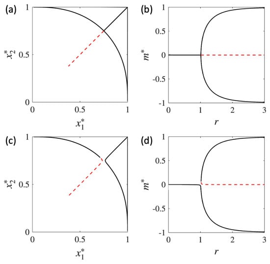
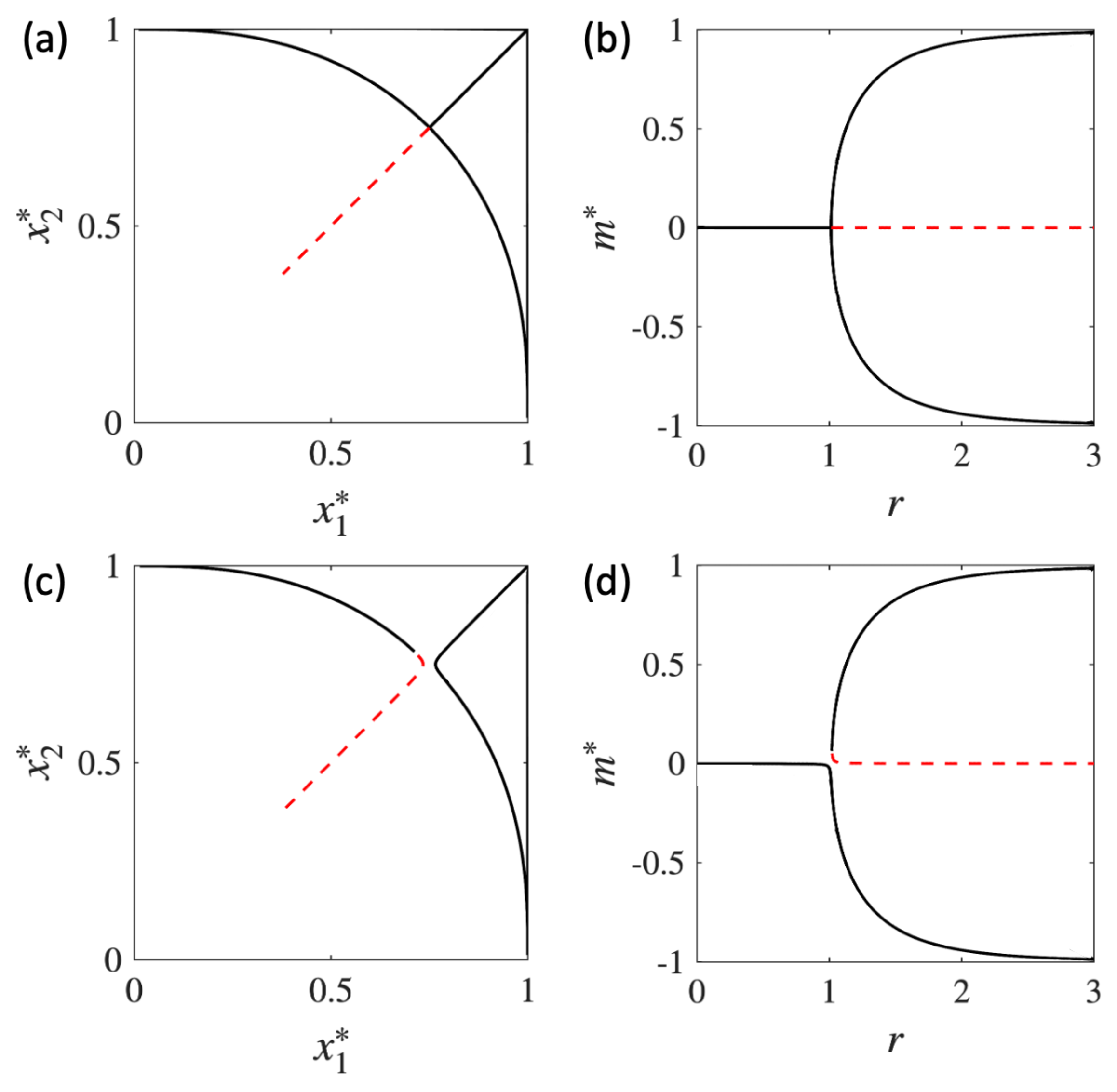
Let us first analyze a simplistic scenario where the sets of parameters are equal for both factors, i.e., $\{{\alpha }_1,{\beta }_1\}=\{{\alpha }_2,{\beta }_2\}=\{1.5,1.5\}$. The equilibrium points of the system, $(x_1^{*},x_2^{*})$, for different values of the control parameter r are presented in Figure 2a. For $r<1.012$, the system has a single stable equilibrium point $x_1^{*}=x_2^{*}$. This equilibrium corresponds to a highly symmetric stem cell state, denoted by $C_0$, in which the cell expresses both factors equally. This symmetric state becomes unstable when $r>1.012$, leading to the emergence of two new stable branches of equilibrium points. The stable branch with $x_1>x_2$ or $x_1<x_2$ represents cells that overexpress the factor $F_1$ or $F_2$, respectively. Let us denote these two cells as $C_1$ ($x_1>x_2$) or $C_2$ ($x_1<x_2$). The new cells function in a lower-symmetry state, as they primarily express only one factor. This stability analysis resembles the standard supercritical pitchfork bifurcation.

Figure 2. Bifurcation diagrams for the biochemical switch model defined by Equations (1) and (2). For panels (a,b), ${\alpha }_1={\alpha }_2=1.5$ and ${\beta }_1={\beta }_2=1.5$. For panels (c,d), the parameters values are the same as in (a,b), except that ${\beta }_2=1.501$.

A more convenient way to describe this transition is by defining the order parameter:

$$m=x_2-x_1.$$

(3)

In this representation, the state with $m=0$ corresponds to the stem cell, $C_0$, and the states with $m<0$ or $m>0$ represent cells $C_1$ or $C_2$, respectively. Figure 2b clearly shows that this transition is a supercritical pitchfork bifurcation [24]. At the bifurcation point, $(m^{*},r^{*})=(0,1.012)$, a symmetry-breaking event occurs, causing the system to transition from a higher symmetric state ($C_0$) to a lower symmetric state ($C_1$ or $C_2$). Mathematically, this symmetry-breaking event represents stem cell differentiation.

The supercritical pitchfork bifurcation presented in Figure 2a,b is only possible because the set of parameters is identical for each factor. A small perturbation of ${\beta }_2$, for instance, breaks the symmetry of the pitchfork bifurcation and gives rise to a pair of saddle–node bifurcations in parameter space. This is clear in Figure 2c,d, which show the stability analysis of the system if we increase the degradation rate of $F_2$ by 0.001, i.e., ${\beta }_2=1.501$. In both figures, the perfect symmetry of the pitchfork bifurcations has been altered and replaced by a stable branch of equilibrium points and a saddle-node bifurcation. The altered bifurcation diagrams correspond to a one-parameter slice of a cusp bifurcation. The order parameter m describes a stem cell state at $m=0$ and the specialized cell states $C_1$ and $C_2$ for positive and negative values of m, respectively.

3. Self-Regulated Biochemical Switch

The supercritical pitchfork and saddle-node bifurcations shown in Figure 2 can only occur when the external input, r, is manually decreased from $r>1.012$ to $r<1.012$. In one of our recent publications [11], we demonstrated that a dynamical system exhibiting a supercritical pitchfork bifurcation can evolve from a single stable equilibrium, autonomously cross the bifurcation point, and asymptotically settle on one of the two stable branches that emerge beyond it. This transition is driven by a feedback mechanism that represents the impact of epigenetic factors on the control parameter r [5,11]. Building on this work, we assume that r is regulated by the following feedback mechanism:

$${\displaystyle \frac{dr}{dt}}=G(M^2-m^2-Ar).$$

(4)

This equation is commonly used to describe physical systems exhibiting self-organized criticality (see, for example, [25]). In these systems, the evolution of the control parameter is governed by an interplay between external driving and internal feedback. In the present model, r is driven upward at a constant rate B by an external source, which may represent environmental or epigenetic inputs. At the same time, r is driven downward by both the system’s internal activity, quantified by $m^2$, and its own intrinsic relaxation. These assumptions are captured by $\dot{r}=B-G{m}^2-gr$, where G and g are rate constants. Through this feedback mechanism, r adapts to the system’s state and self-tunes the dynamics toward a target regime controlled by the parameter B. The quadratic term in this equation was selected to maintain the $m\to -m$ invariance of the pitchfork bifurcation. By rescaling the parameters according to $M^2=B/G$ and $A=g/G$, we arrive at Equation (4). In this form, $M^2$ sets the target level of internal activity toward which the system self-tunes, while A controls its intrinsic relaxation. The parameter G controls the overall relaxation timescale of the activity-dependent feedback acting on the control parameter r. Although G could be removed by rescaling the kinetic parameters (${\alpha }_i$, ${\beta }_i$) and measuring time in units of $G^{-1}$, we retain it explicitly. This is essential in the multiple coupled biochemical switches presented below, as it allows each unit to have distinct feedback and relaxation timescales. In the present single biochemical switch model, we fix $G=0.05$ and $A=1.5$ to allow direct comparison with the original biochemical switch model. In what follows, we will discuss how the three-dimensional dynamical system represented by Equations (1), (2), and (4) can model the differentiation of a stem cell into two progenitor cells.

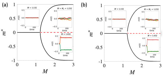
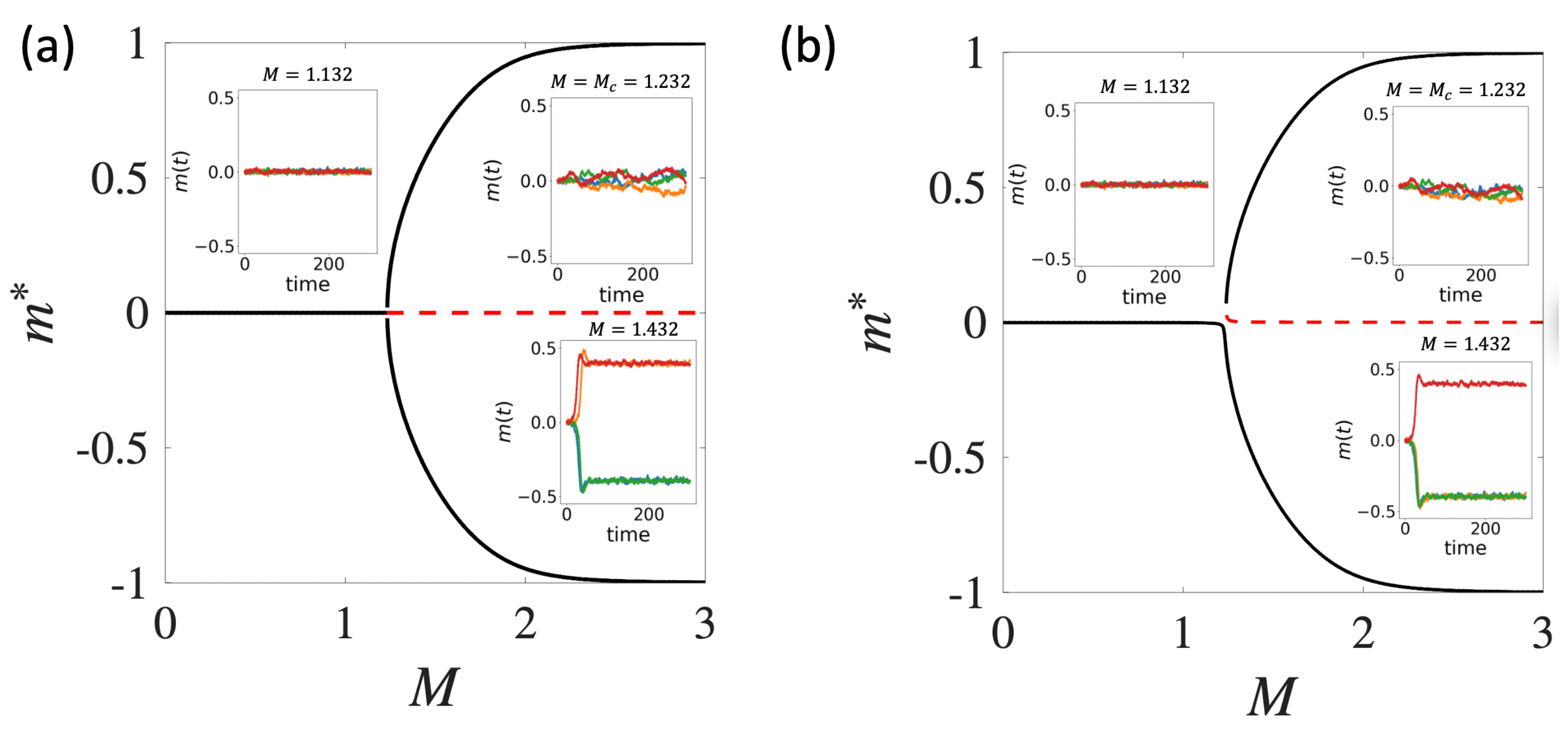
The equilibrium points $(m^{*},r^{*})$ are computed as functions of the control parameter M, with a critical transition occurring at $M_c=1.232$. The corresponding bifurcation diagrams $m^{*}\left(M\right)$ for the two parameter sets are shown in Figure 3a,b. The stability branches for $r^{*}$ can be obtained by substituting $m^{*}\left(M\right)$ into $\dot{r}=0$, yielding $r^{*}=[M^2-{\left(m^{*}\right)}^2]/A$. Since the focus here is on the behavior of the order parameter $m^{*}$, the corresponding $r^{*}\left(M\right)$ diagrams are omitted. Importantly, Figure 3a,b demonstrate that introducing the feedback mechanism in Equation (4) does not qualitatively alter the structural stability of the system. The organization of the $m^{*}$ branches and their transitions remains topologically equivalent to the case in which the control parameter, r, is static (see Figure 2b,d). Consequently, the self-regulated biochemical switch also predicts transitions from the pluripotent state $C_0$ to the differentiated states $C_1$ or $C_2$, as described by the analysis in the previous section.

Figure 3. Bifurcation diagrams for the biochemical switch model defined by Equations (1), (2), and (4). Parameters in (a) match those in Figure 2b, and parameters in (b) are the same as in Figure 2d. Furthermore, both subfigures have $G=0.05$ and $A=1.5$.

The present deterministic model can be readily extended to include stochastic fluctuations arising from finite-size effects and gene expression variations [26,27]. The mathematical formulation and numerical solution of the stochastic dynamical system are detailed in Appendix A.1 [28]. Examples of representative stochastic trajectories in the vicinity of the critical point $M_c$ are shown in the insets of Figure 3a,b. In these simulations all initial conditions represent the pluripotent state, i.e., $m=0$ and $r<1$. For $M<M_c$, stochasticity remain small and the system fluctuates around a single stable equilibrium. As M approaches $M_c$, the amplitude of fluctuations increases considerably, reflecting enhanced sensitivity near the bifurcation. For $M>M_c$, trajectories branch and relax toward the newly formed stable equilibrium states, as expected for a pitchfork bifurcation. In the asymmetric case, the effective potential is biased in favor of $x_1$. Consequently, for $M>M_c$ the system is more likely to approach the equilibrium branch with $m^{*}<0$.

Next, we will explore how the feedback mechanism allows the dynamical system to start at a pluripotent stem cell state and autonomously navigate through the bifurcation point, where the spontaneous symmetry-breaking event occurs. To illustrate this successfully, we will numerically construct the corresponding part of the epigenetic landscape using the concept of quasi-potential [29],

$$\Phi (m,t)\propto -log\left[P\right(m,t\left)\right],$$

(5)

where $P(m,t)$ is the probability of finding the system at state m at time t. The construction and sensitivity analysis of the probability distribution $P(m,t)$ are given in Appendix A.2. Unless otherwise stated, the variance of white noise was maintained at $\sigma =0.005$. It is important to note that this approach may not fully capture the potential landscape due to the extremely rare occurrence of certain stable solutions. Unavoidably, such states will be represented by infinite $\Phi (m,t)$. Here, these rare states are referred to as silenced states within a fixed number of independent simulations. In this context, they correspond to cells that rarely express specific genes, a phenomenon known as gene silencing [30].

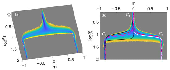
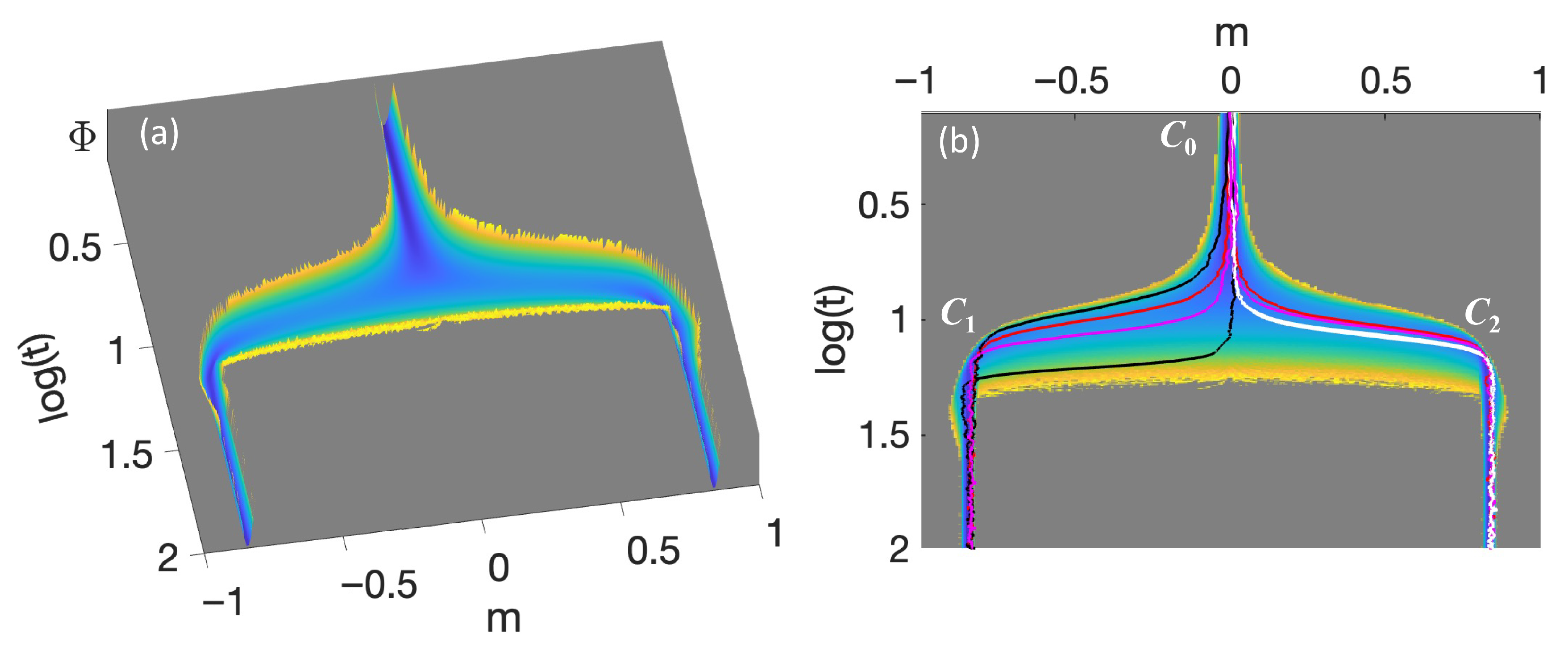
Figure 4a shows the three-dimensional plot of the quasi-potential for the values of parameters used in Figure 3a. It is evident that $\Phi (m,t)$ qualitatively resembles the first decision-making event of Waddington’s epigenetic landscape, i.e., the differentiation of the stem cell to two progenitors (see Figure 1b). The corresponding density plot of the quasi-potential with eight randomly selected simulated trajectories embedded is shown in Figure 4b. It is clear that all trajectories starting from the pluripotent stem cell state approach the bifurcation point and then, due to randomness, spontaneously follow either the $C_1$ or $C_2$ branch. We observed no transitions from $C_1$ to $C_2$ for this level of randomness. Such transition will indicate a direct reprogramming of the cell and will be discussed in Section 5. Note that the details of the quasi-potential, including the depth and width of the well, can be adjusted by modifying the parameters of the dynamical system. This process is quite complex and delicate, and it will be addressed in the following sections.

Figure 4. (a) Three-dimensional plot and (b) density plot of the quasi-potential $\Phi (\mathcal{M},t)$. In (b), eight random differentiation trajectories are also embedded in the density. The parameters used are the same as those in Figure 3a. Density colors represent increasing $\Phi$ values, ranging from blue (lowest), through green and yellow, to gray (highest).

4. Hierarchically Coupled Biochemical Switches

Following our recent works [11,28], we assume that a pluripotent stem cell consists of n hierarchically coupled modules. Each module is modeled by a self-regulated dynamical system discussed in Section 3. Mathematically, the dynamics of the $i_{\mathrm{th}}$ module are described by

$${\displaystyle \frac{d{x}_{1i}}{dt}}={\displaystyle \frac{{\alpha }_{1i}}{1+{\left(r_i{x}_{2i}\right)}^4}}-{\beta }_{1i}{x}_{1i},$$

(6)

$${\displaystyle \frac{d{x}_{2i}}{dt}}={\displaystyle \frac{{\alpha }_{2i}}{1+{\left(r_i{x}_{1i}\right)}^4}}-{\beta }_{2i}{x}_{2i},$$

(7)

$${\displaystyle \frac{d{r}_i}{dt}}=G_i(M_i^2-m_i^2-A_i{r}_i),$$

(8)

where $m_i=x_{2i}-x_{1i}$.

Depending on the value of $M_i$, each module can be activated and assume one of the possible stable attractors with $m_i^{*}>0$ or $m_i^{*}<0$. Similarly to [11], the activation of each module happens sequentially through a very simple hierarchical coupling. Specifically, for $i=1$

$$M_1={\overline{M}}_1+\sum _{j=1}^n{d}_{1j}{m}_j,$$

(9)

while for $i>1$,

$$M_i=\sum _{j=1,j<i}^n{c}_{ij}{m}_j+\sum _{j=1}^n{d}_{ij}{m}_j.$$

(10)

Initially, all modules are in their inactive state ($m_i=0$, $r_i<1$). At this stage, all $M_i=0$, except for $M_1={\overline{M}}_1$. One major assumption of this work that was mentioned earlier, is that the parameter ${\overline{M}}_1$ is controlled by epigenetic factors. Over time, the first module crosses the bifurcation point and transitions to one of its two stable attractors. We refer to this transition as the activation of the module. Once $m_1\ne 0$, $M_2$ gradually takes on non-zero values that trigger the differentiation of the second module. Eventually, each module drives the differentiation of the next module in a sequential manner. Once all modules are activated the differentiation process concludes.

Technically, this hierarchical activation is achieved if the elements of the matrix $\mathbf{c}=c_{ij}$ are non-zero only for $j<i$ (i.e., $\mathbf{c}$ is a strictly lower triangular matrix). The matrix $\mathbf{d}=d_{ij}$ provides weak coupling between different modules simultaneously. For simplicity, we assume that the diagonal elements of $\mathbf{d}$ are all zero, meaning there is no additional self-regulation apart from the $m_i^2$ term in Equation (4). As it will be demonstrated below, the interaction strengths $d_{ij}$ and the parameters ${\alpha }_{ki}$ and ${\beta }_{ki}$, where $k=1,2$, introduce the necessary asymmetry to make the system more realistic and tunable.

Similarly to the previous section, transcriptional noise is represented by adding a stochastic term ${\sigma }_{ji}d{W}_t^{\left(ji\right)}$ to each differential $d{x}_{ji}$ in Equations (6) and (7), where $j=1,2$ and $i=1,\dots ,n$. All Wiener processes $W_t^{\left(ji\right)}$ are independent. The standard deviations ${\sigma }_{ji}$ are presented in Table 1. The numerical solution of the stochastic differential equations is presented in Appendix A.1.

At any given time, t, the system is characterized by the state vector

$$\mathbf{m}\left(t\right)=\{m_1\left(t\right),m_2\left(t\right),\dots ,m_n\left(t\right)\}.$$

The n—dimensional state space is projected into a single coordinate [11]:

$$\mathcal{M}\left(t\right)=m_1\left(t\right)+m_2\left(t\right)+\cdots +m_n\left(t\right).$$

(11)

This projection is introduced as a generic, low-dimensional coordinate to visualize hierarchical progression along the epigenetic landscape in the spirit of Waddington’s original representation. This reduction is not intended to, and cannot, uniquely represent the full high-dimensional state of the system. In particular, distinct trajectories in the full state space may project onto similar values of $\mathcal{M}\left(t\right)$, giving the appearance of overlapping paths. Such overlaps do not imply degeneracy or the existence of multiple solutions, but rather reflect the loss of information associated with projecting high-dimensional dynamics onto a single coordinate. Therefore, the use of $\mathcal{M}\left(t\right)$ provides a simple, intuitive picture of the developmental process, while the full dynamics remain high-dimensional.

Note that each module starting from the state $m_i\left(t\right)=0$ will eventually approach one of the two possible attractors, i.e., $m_i\left(t\right)\to m_i^{*}\in \{m_i^{*}>0,m_i^{*}<0\}$, as $t\to \infty$. For convenience, let us define the index $s_i=0,1,$ or 2 for $m_i=0$, $m_i<0$, or $m_i>0$, respectively. Thus, at any time t, the state of the cell can be denoted by $C_{s_1{s}_2\dots s_n}$. In the long run, all $s_i$ will be either 1 or 2. In this case, the system has reached one of the $2^n$ attractors:

$${\mathcal{M}}_{s_1{s}_2...s_n}=m_1^{*}+m_2^{*}+\cdots +m_n^{*}.$$

(12)

that correspond to specialized cells $C_{s_1{s}_2...s_n}$.

For example, for $n=3$, the state $C_{000}$ corresponds to the pluripotent stem cell states where none of the modules is activated ($m_1\left(t\right)=m_2\left(t\right)=m_3\left(t\right)=0$). Similarly, the state $C_{100}$ and $C_{200}$ correspond to a progenitor, where only the first module is differentiated with $m_1^{*}<0$ and $m_1^{*}>0$, respectively. The state $C_{121}$ corresponds to a specialized cell where all three modules are differentiated ($m_1^{*}<0$, $m_2^{*}>0$, and $m_3^{*}<0$). Overall, the system will undergo three differentiations at times $t_1$, $t_2$, $t_3$, leading to the creation of the following cells:

$$\begin{array}{cc}\hfill \{& \left\{C_{000}\right\}\stackrel{t_1}{\to }\{C_{100},C_{200}\}\stackrel{t_2}{\to }\{C_{110},C_{120},C_{210},C_{220}\}\stackrel{t_3}{\to }\hfill \\ \hfill & \{C_{111},C_{112},C_{121},C_{122},C_{211},C_{212},C_{221},C_{222}\}\}.\hfill \end{array}$$

Note that eventually ($t>t_3$), the system will reach one of the 8 ($2^3$) attractors,

$${\mathcal{M}}_3^{*}=\{{\mathcal{M}}_{111},{\mathcal{M}}_{112},{\mathcal{M}}_{121},{\mathcal{M}}_{122},{\mathcal{M}}_{211},{\mathcal{M}}_{212},{\mathcal{M}}_{221},{\mathcal{M}}_{222}\},$$

each of which will represent one of the following specialized cells,

$${\mathcal{C}}_3=\{C_{111},C_{112},C_{121},C_{122},C_{211},C_{212},C_{221},C_{222}\}.$$

In general, the state $C_{000}$ represents the most upstream cell state explicitly resolved in the model and may correspond either to a pluripotent stem cell or an early progenitor. Cells in this state co-express multiple lineage-associated transcription factors. The first modeled fate decision, governed by the initial biochemical switch, corresponds to the selective activation of a specific lineage module.

In hematopoietic contexts, activation of the PU.1-GATA1 module defines an early hematopoietic progenitor state, $C_{100}$, while activation of a parallel lymphoid commitment module, such as Pax5-EBF1, defines a B-lineage progenitor state, $C_{200}$. These modules operate at a comparable hierarchical level but govern distinct branches of the hematopoietic differentiation tree [31,32].

If the PU.1-GATA1 module is selected, a subsequent fate decision is governed by a downstream biochemical switch that leads to either a PU.1-dominant myeloid state ($C_{110}$) or a GATA1-dominant erythroid state ($C_{120}$). Further downstream differentiation can be represented by additional modules, such that $C_{121}$ corresponds to a more specific myeloid subtype, while $C_{122}$ represents a mature erythroid state. In contrast, activation of the Pax5–EBF1 module results in the formation of committed B-lineage progenitors. When Pax5–EBF1 is not active, the cell remains uncommitted and retains the ability to differentiate into alternative lymphoid lineages. These lineage-committed progenitor states may then undergo additional downstream fate decisions before reaching terminal differentiation.

4.1. Symmetric Hierarchical Branching

In this section, we will discuss the construction of the quasi-potential. We will examine only the case of three modules ($n=3$) and, for simplicity, use identical parameters for each module (see Table 1). The selection of these parameters is discussed in Appendix A.3. All simulations start from the pluripotent stem cell state, i.e., the initial conditions are $x_{1i}=x_{2i}=1$ (i.e., $m_i=0$) and $r_i=0.8$.

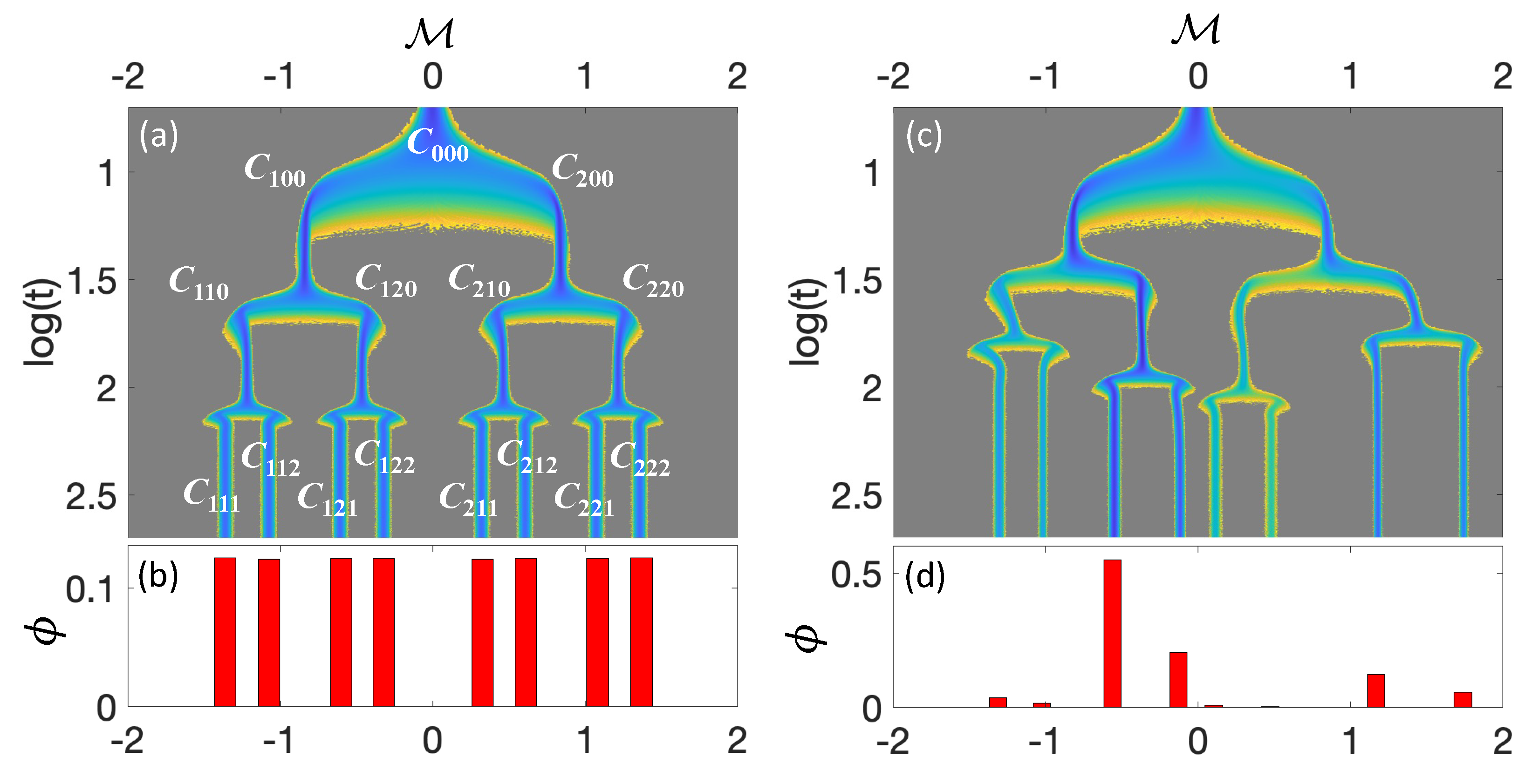
The top of Figure 5a shows the density plots of the quasi-potential. Initially, the system is in the ${\mathcal{M}}_{000}=0$ state, where all $m_i\approx 0$. This state corresponds to an undecided pluripotent stem cell, $C_{000}$. Subsequently, at time $t_1\approx 8$, the first module gets activated and spontaneously chooses one of the two attractors $m_1^{*}\approx \pm 0.84$. This activation splits the initial single well of $\Phi (\mathcal{M},t)$ into two transiently stable branches that correspond to the multipotent progenitor cells $C_{100}$ and $C_{200}$. After some time ($t_2\approx 35$), the second module also gets activated ($m_2^{*}\approx \pm 0.38$), leading to the formation of four transiently stable branches. These branches correspond to cells $C_{110}$, $C_{120}$, $C_{210}$, and $C_{220}$, which may be interpreted as oligopotent progenitors, i.e., progenitors that are more committed to specific lineages. Finally, after time $t_3\approx 125$, the third module gets activated and assumes one of the two attractors $m_3^{*}\approx \pm 0.14$. This last activation results in eight asymptotically stable branches, which correspond to eight different specialized cells ${\mathcal{C}}_3$. At this point, the differentiation process is complete. The fractions of each produced cell can be estimated by

$$\varphi \left(M\right)={\int }_{M-ϵ}^{M+ϵ}P(\mathcal{M},t)d\mathcal{M},$$

(13)

where $t>t_3$, $M\in {\mathcal{M}}_8^{*}$ and $ϵ$ is a positive real number, such that $P(M\pm ϵ,t)\approx 0$. These fractions are shown in Figure 5b.

Figure 5a,b highlight two interesting properties of this model, both of which originate from the specific parameter values described in Table 1. These parameters lead to a perfect supercritical pitchfork bifurcation for each module, consistent with the analysis presented in Figure 3a. First, the distribution of fractions is uniform, clearly demonstrating that the differentiation process produces an equal quantity of each cell type. Second, the attractors exhibit an apparent symmetry along the generic coordinate state $\mathcal{M}$. For example, ${\mathcal{M}}_{111}=-{\mathcal{M}}_{222}$ or ${\mathcal{M}}_{112}=-{\mathcal{M}}_{221}$. This symmetry in the state space arises from the quadratic term in Equation (8), which preserves the characteristic invariance $m_i\to -m_i$ of the pitchfork bifurcation. Consequently, the system also remains invariant under $\mathcal{M}\to -\mathcal{M}$.

Table 1. This example serves as an idealized representation of cell differentiation and was used solely to illustrate the potential of the proposed hierarchical model.

	$i=1$	$i=2$	$i=3$	$\mathbf{c}=\left(\begin{array}{ccc}0& 0& 0\\ 0.5& 0& 0\\ 0& 0.4& 0\end{array}\right),\mathbf{d}=0$
${\alpha }_{1i}={\alpha }_{2i}$	$1.5$	$1.5$	$1.5$
${\beta }_{1i}={\beta }_{2i}$	$1.5$	$2.25$	$3.0$
${\sigma }_{1i}={\sigma }_{2i}$	$0.005$	$0.005$	$0.005$
$G_i$	$0.05$	$0.25$	$0.75$
$A_i$	1.5	0.02	0.001
${\overline{M}}_i$	$\sqrt{3}$	-	-

Table 1. This example serves as an idealized representation of cell differentiation and was used solely to illustrate the potential of the proposed hierarchical model.

	$i=1$	$i=2$	$i=3$	$\mathbf{c}=\left(\begin{array}{ccc}0& 0& 0\\ 0.5& 0& 0\\ 0& 0.4& 0\end{array}\right),\mathbf{d}=0$
${\alpha }_{1i}={\alpha }_{2i}$	$1.5$	$1.5$	$1.5$
${\beta }_{1i}={\beta }_{2i}$	$1.5$	$2.25$	$3.0$
${\sigma }_{1i}={\sigma }_{2i}$	$0.005$	$0.005$	$0.005$
$G_i$	$0.05$	$0.25$	$0.75$
$A_i$	1.5	0.02	0.001
${\overline{M}}_i$	$\sqrt{3}$	-	-

Figure 5. (a) Density plot of $\Phi (\mathcal{M},t)$ for the symmetric case. Subfigure (b) shows the corresponding ratios, $\varphi$, of the specialized cells produced. Subfigures (c,d) present the density plot of $\Phi (\mathcal{M},t)$ and the corresponding cell ratios for the asymmetric case. In (a,b), the parameters are given in Table 1. The parameter values in (c,d) are identical to those in (a,b), except that the coefficients ${\beta }_{li}$ and the matrix d are defined according to Equations (14) and (15), respectively. Density color indicates increasing $\Phi$ values, ranging from blue (lowest), through green and yellow, to gray (highest).

Figure 5. (a) Density plot of $\Phi (\mathcal{M},t)$ for the symmetric case. Subfigure (b) shows the corresponding ratios, $\varphi$, of the specialized cells produced. Subfigures (c,d) present the density plot of $\Phi (\mathcal{M},t)$ and the corresponding cell ratios for the asymmetric case. In (a,b), the parameters are given in Table 1. The parameter values in (c,d) are identical to those in (a,b), except that the coefficients ${\beta }_{li}$ and the matrix d are defined according to Equations (14) and (15), respectively. Density color indicates increasing $\Phi$ values, ranging from blue (lowest), through green and yellow, to gray (highest).

4.2. Asymmetric Hierarchical Branching

The symmetric case studied in the previous subsection was introduced as a minimal setting in which the mechanism of symmetry breaking can be analyzed transparently. Although it is intuitively useful, exact symmetry between competing states is not very likely to happen in biological systems, where molecular interactions and regulatory processes inevitably introduce biases. As a result, distinct cell fates are not expected to be equivalent in either stability or accessibility. To account for this, the symmetry assumption is relax to enables the construction of epigenetic landscapes that more closely reflect realistic differentiation scenarios, in which one fate may be favored over another.

Here, the parameters $\left\{{\beta }_{ji}\right\}$ and the interaction matrix $\mathbf{d}$ in Table 1 are replaced, respectively, by

$$\left\{{\beta }_{ji}\right\}=\left(\begin{array}{ccc}{\beta }_{11}& {\beta }_{12}& {\beta }_{13}\\ {\beta }_{21}& {\beta }_{22}& {\beta }_{23}\end{array}\right)=\left(\begin{array}{ccc}1.4885& 2.2455& 2.9975\\ 1.5015& 2.2525& 3.0005\end{array}\right)$$

(14)

and

$$\mathbf{d}=\left(\begin{array}{ccc}0& -0.2986& -0.2337\\ 0.1513& 0& -0.1804\\ 0.0595& 0.0463& 0\end{array}\right).$$

(15)

The perturbation of ${\beta }_{ji}$ replaces the supercritical pitchfork bifurcations of the previous example with a stable branch and two saddle node bifurcations. As shown in Figure 3b, this process can still generate two stable branches for each module: one with $m_i^{*}>0$ and one with $m_i^{*}<0$. However, the overall potential function is tilted, resulting in branches with lower potential function values. The new landscape favors specific differentiation paths, and, as a result, the creation of certain cell types is more probable. This analysis is clearly illustrated in the density plot of the quasi-potential and fractions distributions in Figure 5c. The differentiation path $C_{000}\to C_{100}\to C_{120}\to C_{121}$ corresponds to deeper $\Phi (\mathcal{M},t)$, indicating that the terminal cell $C_{121}$ is more likely to occur. This is also evident in the fractions distribution (see, Figure 5d), where ${\mathcal{C}}_{121}$ clearly receives the largest proportion.

Interestingly, some regions of the quasi-potential correspond to stable attractors that are rarely visited. This occurs because these attractors lie at much higher quasi-potential values than the dominant states, making them statistically unlikely to be occupied despite being locally stable. Similar rare but stable attractor states have been proposed in the literature as a conceptual framework for abnormal or pathological cellular activity, including cancer states, which may arise from noise-driven transitions in GRN [33]. In the present work, this interpretation is offered only as a qualitative analogy, and no explicit cancer-specific mechanisms are modeled.

Another noteworthy observation is the alteration of state symmetry. While the system still produces eight possible cell types, the state space symmetry of the corresponding attractors has been eliminated.

5. Reprogramming

In this section, we will discuss how the proposed model can describe transdifferentiation, dedifferentiation, or reprogramming of a specialized cell [34,35,36]. Transdifferentiation or direct reprogramming is the process of transforming a cell type directly into another without undergoing intermediate cell states [34,36]. For instance, $C_{222}\to C_{221}$ would be considered transdifferentiation in our model. This type of reprogramming can be achieved by environmental factors or by introducing specific transcription factors such as Ascl1, Brn2, and Myt1l for neuronal reprogramming [21]. Dedifferentiation, on the other hand, refers to the process where a specialized cell transiently becomes a progenitor-like cell with limited potency within the same lineage before differentiating into a different specialized cell, e.g., $C_{222}\to C_{220}\to C_{221}$. Dedifferentiation is usually achieved by exposure to injury signals, environmental stress, or specific epigenetic modifiers such as histone deacetylase inhibitors [35]. In reprogramming, a specialized cell restores its full pluripotency, i.e., it becomes a pluripotent stem cell, which can then differentiate into any possible cell type. In our model, a $C_{222}\to C_{000}\to C_{100}\to C_{120}\to C_{121}$ would be considered a reprogramming process. Induced pluripotent stem cells can be produced in the lab by introducing Yamanaka factors (Oct4, Sox2, Klf4, and c-Myc) [22].

The silencing and overexpression interventions considered in this section are intended as abstract representations of experimentally established reprogramming strategies. For example, strong overexpression of lineage-defining transcription factors, such as Ascl1 in neuronal reprogramming, can be viewed within the present framework as parameter changes that destabilize existing attractors and bias the landscape toward a specific target fate. In contrast, overexpression of the Yamanaka factors effectively returns the system toward an upstream bifurcation point in the developmental landscape, where multiple fates again become accessible. This resets lineage commitment and leads to heterogeneous and probabilistic reprogramming outcomes. In this sense, the modeled interventions describe generic dynamical effects of known reprogramming factors without aiming to represent their detailed biochemical mechanisms.

To incorporate transient external effects in our model, it is essential to introduce the sigmoid step function

$$H_{(t_a,t_b)}={\displaystyle \frac{1}{1+e^{-\lambda (t-t_a)}}}-{\displaystyle \frac{1}{1+e^{-\lambda (t-t_b)}}},$$

(16)

where the times $t_a<t_b$ determine the interval of the intervention $[t_a,t_b]$. Note that $t_a$ must always be greater than the time needed for the initial differentiation of the stem cell, i.e., greater than $t_a>t_3$. Here, $\lambda$ is the steepness parameter that controls the rate at which the function transitions from 0 to 1 or vice versa. Unless otherwise stated, $t_a=250$, $t_b=300$, and $\lambda =0.25$. The reprogramming efficiency is measured by the ratio:

$$E={\displaystyle \frac{N_{\mathrm{s}}}{N_{\mathrm{tot}}}},$$

(17)

where $N_{\mathrm{tot}}$ is the total number of realizations and $N_{\mathrm{s}}$ is the number of successfully reprogrammed states. For simplicity, we will exclusively use the symmetric stem cell model presented in Figure 5a. It is important to emphasize that the reported efficiencies of the interventions strongly depend on the parameters $\lambda$, $t_a$, and $t_b$.

5.1. Dedifferentiation and Reprogramming

We will begin by discussing how the proposed model can describe partial or full restoration of pluripotency. Let us first recall that once the ${(i-1)}_{\mathrm{th}}$ module is activated, it directs the activation of the $i_{\mathrm{th}}$ module through $M_i$ (see Equations (9) and (10)). Thus, if one can temporarily silence $M_i$(≈0), then $i_{\mathrm{th}}$ module will gradually transition back to the inactive state ($m_i\approx 0$) allowing the cell to partially recover potency corresponding to the immediate upstream state. This approach can be mathematically represented as:

$$M_i\left(t\right)\mapsto M_i\left(t\right)(1-f_i{H}_{(t_a,t_b)}),$$

(18)

where $f_i\in [0,1]$ is the efficiency of silencing the expression of the $i_{th}$ module’s activating factor.

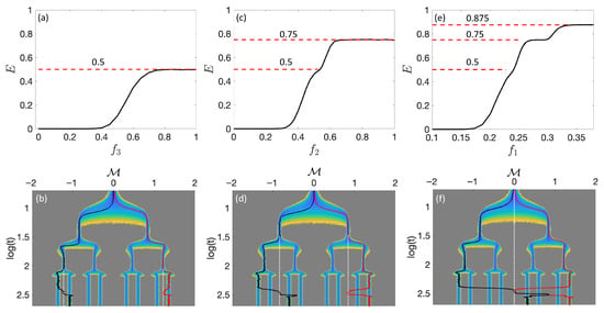
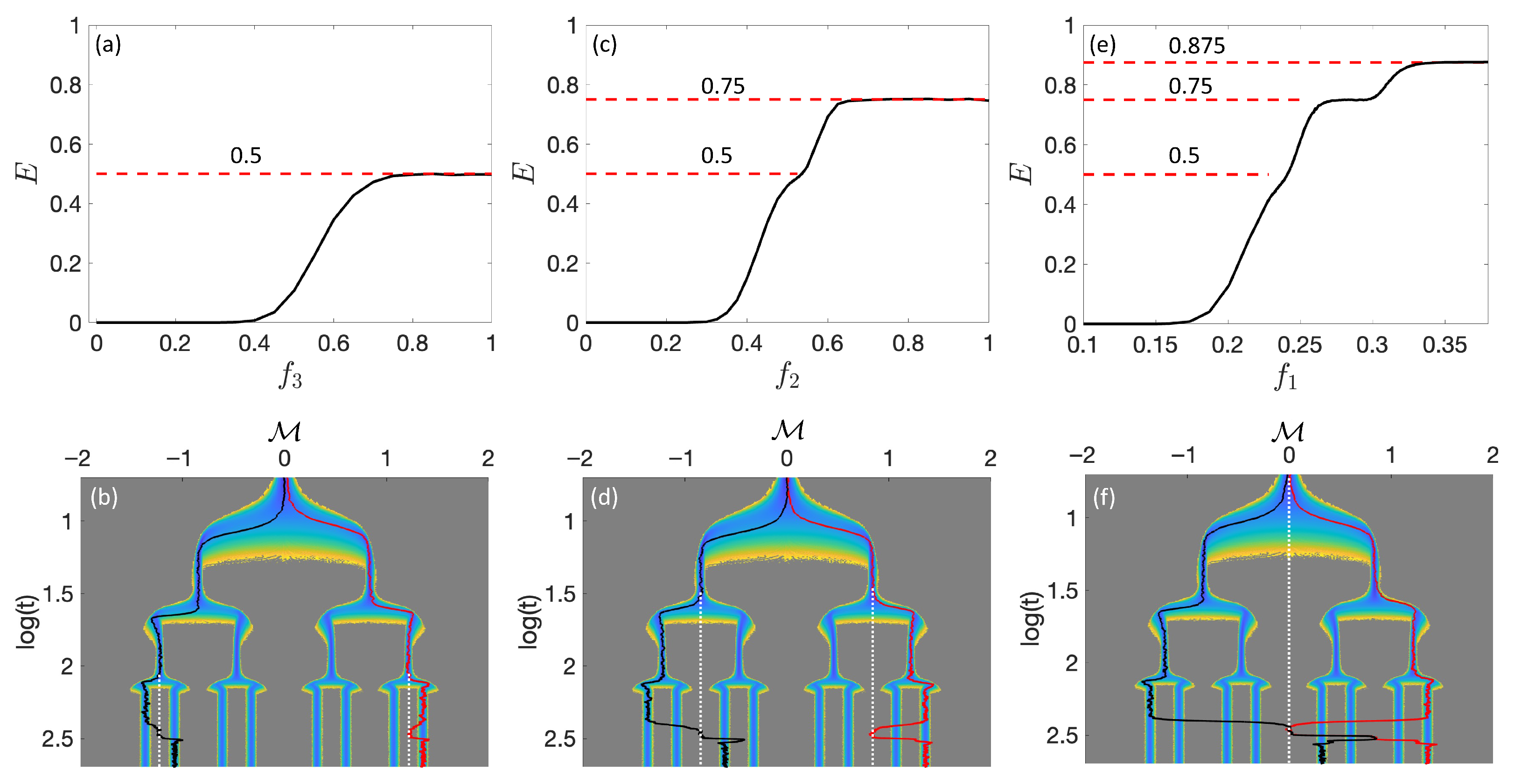
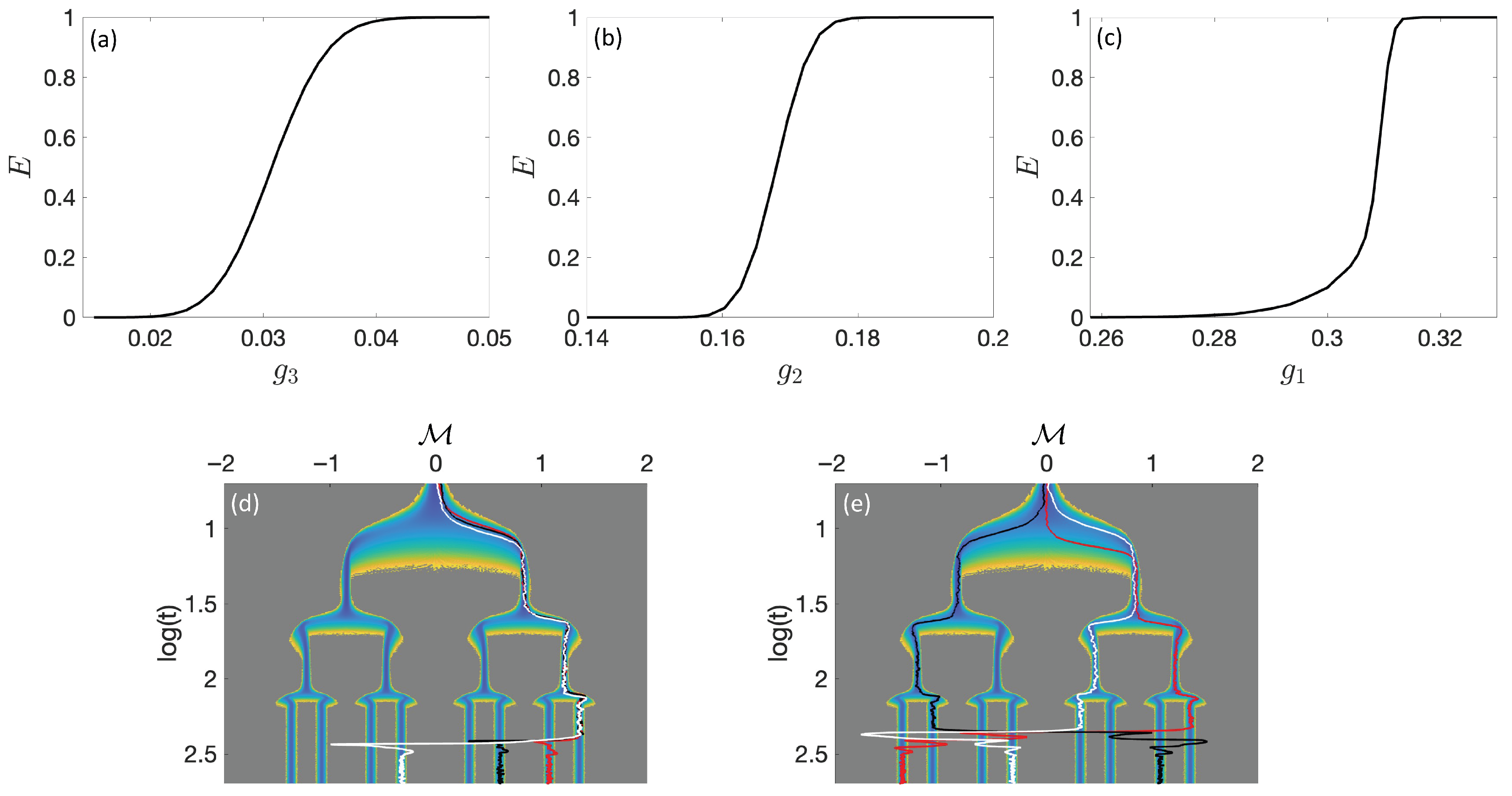
We will begin our analysis by examining the effects of silencing $M_3$. In this case, the third module will gradually achieve its inactive state $m_3\approx 0$. For instance, a cell $C_{222}$ may temporarily transition to $C_{220}$, thereby effectively reverting to a state of an oligopotent progenitor. Once the intervention is turned off, the cell can spontaneously differentiate back into either $C_{221}$ or $C_{222}$. Since we chose to focus on the symmetric cell differentiation shown in Figure 5a, the maximum reprogramming efficiency cannot exceed the value of $0.5$. Figure 6a shows the efficiency of reprogramming versus $f_3$. Note that E starts from zero and gradually increases to the maximum value of 0.5 for $f_i\gtrsim 0.8$. Figure 6b demonstrates one successful and one unsuccessful attempt to partially reprogram a cell. For instance, the black trajectory demonstrates an initially differentiated $C_{111}$ cell. At time $t_a$, where the intervention begins, the third module reaches the inactive state $C_{110}$ (see dashed white line). Subsequently, it successfully differentiates into $C_{112}$ once the intervention is switched off at time $t_b$. The red line describes an unsuccessful dedifferentiation trajectory. Although the cell started from a $C_{222}$ and successfully reverted into a $C_{220}$ (dashed white line), it eventually differentiated again into $C_{222}$ state. This is characterized as an unsuccessful dedifferentiation process.

Figure 6. Panels (a,b) correspond to the silencing of factor $M_3$. Specifically, (a) shows the reprogramming efficiency, E, as a function of the silencing strength $f_3$, while (b) presents representative trajectories from successful (black lines) and unsuccessful reprogramming attempts. Panels (c,d) show the corresponding results for silencing factor $M_2$, and panels (e,f) for factor $M_1$, following the same layout. The values of the parameters are given in Table 1. In (b,d,f), density color indicates increasing $\Phi$ values, ranging from blue (lowest), through green and yellow, to gray (highest).

We continue by discussing the effects of silencing $M_2$. Here, depending on the values of $f_2$, the cell $C_{222}$ may either transition to $C_{220}$, $C_{202}$, or $C_{200}$. The first two transitions occur for low to intermediate values of $f_2$, where intervention is not strong enough to fully restore the progenitor state ($C_{200}$). The third transitions indicates full restoration of the progenitor state and occurs only for strong values of $f_2$. Once this state is achieved, the cell can differentiate into the four available cell states within the same lineage. Therefore, the maximum efficiency of reprogramming is $0.75$. Figure 6c demonstrates the efficiency of reprogramming versus $f_2$. Notably, for large values of $f_2$ ($\gtrsim 0.65$), the efficiency reaches its maximum value (dotted line). Additionally, at approximately $f_2=0.5$, the efficiency reaches a transient plateau with a $E=0.5$ value. These intermediate values of $f_2$ correspond to the earlier discussed scenario where the intervention is either not strong enough or not sustained long enough to fully restore the multipotent progenitor state. Similarly to the previous case, one successful and one unsuccessful dedifferentiation trajectory are displayed in Figure 6d. For instance, the black trajectory demonstrates an initially differentiated $C_{111}$ cell. At time $t_a$, the cell reaches its progenitor state $C_{100}$ (see dashed white line). Once the intervention is switched off, the cell briefly differentiates into $C_{120}$ and then permanetly into $C_{121}$. The red trajectory displays a cell that successfully transitioned from $C_{222}$ into $C_{200}$ and at time $t_a$. However, it was subsequently differentiated again into $C_{222}$, meaning it returned to its original state.

Lastly, we will present the effects of silencing $M_1$. This is the only case that can revert a specialized cell into a pluripotent stem cell $C_{000}$. Ideally, once $M_1$ is silenced, the first module will return to the $m_1\approx 0$. This result will silence $M_2$ and force the second module into the $m_2\approx 0$ state, which will also silence $M_3$ and push the third module back into the $m_3\approx 0$ state. This process corresponds to complete reprogramming into a stem cell and occurs only when $f_1$ is applied with sufficient strength and duration. Once this happens, the cell can differentiate into any of the 8 cell states in ${\mathcal{C}}_3$. Thus, the maximum possible efficiency is $0.875$, which occurs for $f_1\gtrsim 0.3$. However, for low to intermediate values of $f_3$, the cell may only revert to an oligopotent progenitor or progenitor, causing the efficiency to transiently plateau at $0.5$ or $0.75$, respectively. This analysis is depicted in the E vs. $f_1$ profile (see Figure 6e). Figure 6f shows one successful and one unsuccessful reprogrammed trajectory. Note that both cells were inverted into the pluripotent stem cell; however, only the black trajectory was reprogrammed into a different specialized cell.

Similar to the conclusions of [20], our model predicts that dedifferentiation are inherently probabilistic processes. In dynamical systems language, reprogramming drives the system toward an upstream bifurcation point in the quasi-potential, where multiple stable states are accessible. Although successful escape from the original attractor is likely, the potential new attractor cannot be identified with high confidence. Table 2 summarizes the critical values of $f_i$ that maximize differentiation efficiency.

Table 2. Transdifferentiation: The critical strength $f_i$ that give the maximum differentiation efficiency E, for $i=1,2,\mathrm{and}3$.

Module	$\mathit{i}=1$	$\mathit{i}=2$	$\mathit{i}=3$
$f_i\gtrsim$	0.3	0.65	0.8
$\mathrm{Maximum}\mathrm{efficiency}$	$0.875$	$0.75$	$0.5$

5.2. Transdifferentiation or Direct Reprogramming

Direct reprogramming (transdifferentiation) aims to modulate under- or over-expressed genes through the introduction of specific regulatory factors [21,36]. To model this, we will introduce a transient positive rate of expression in Equations (6) or (7) for the underexpressed gene. For instance, if the $x_{ji}$ is underexpressed, the following rate will be added in the corresponding Equation of (6) or (7):

$$R_{ji}\left(t\right)=g_i{H}_{(t_a,t_b)},$$

(19)

where i represents the module index and j the gene factor. Note that $g_i$ controls the strength of expression and is always positive. For instance, let us assume that the the $x_{1i}$ is underexpressed and the state of the $i_{\mathrm{th}}$ module is $m_i^{*}=x_{1i}^{*}-x_{2i}^{*}<0$. This rate will increase $x_{1i}^{*}$ and unavoidably will decrease the expression levels of the $x_{2i}^{*}$. This will transform the cell from the sable attractor $m_i^{*}<0$ to $m_i^{*}>0$.

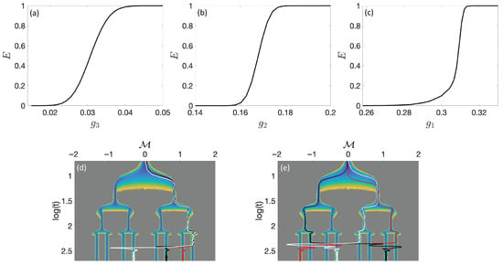
We first study the effect of overexpression in each module separately. Figure 7a–c show the efficiency of reprogramming as a function of $g_3$, $g_2$, and $g_1$, respectively. In all three cases, the reprogramming efficiency E increases gradually with $g_i$ and eventually reaches its maximum value, $E=1$, beyond a critical threshold $g_i=g_i^{\mathrm{cr}}$. For values $g_i<g_i^{\mathrm{cr}}$, the reprogramming process remains probabilistic, in the sense that reprogramming may or may not occur. In contrast, for $g_i\ge g_i^{\mathrm{cr}}$, all cells are successfully reprogrammed, i.e., $E\approx 1$. Table 3 summarizes the critical values of $g_i$ at which transdifferentiation efficiency is maximized. For interventions applied to the third module ($i=3$), successful reprogramming leads to a highly predictable outcome, in contrast to the behavior described in the previous section. For example, a cell initially in state $C_{122}$ transitions to $C_{121}$ with high predictability upon successful reprogramming. Similarly, for interventions on the second module ($i=2$), successful reprogramming converts a $C_{122}$ cell into $C_{112}$. In rare cases, the third module may also switch; however, such events occur with very low probability. Finally, when intervening on the first module ($i=1$), successful reprogramming of a $C_{122}$ cell yields the state $C_{222}$, although downstream modules may still very rarely switch. Overall, while the reprogramming process itself remains probabilistic, the outcome conditioned on success is highly predictable, with a reprogramming efficiency $E\approx 1$. Consequently, the resulting cell fate is substantially more predictable than in the previous section.

Figure 7. Subfigures (a–c) show the reprogramming efficiency, E, versus the intervention strengths, $g_3$, $g_2$, and $g_1$, respectively. Subfigures (d,e) illustrate the trajectories of successful targeted reprogramming (see text for details). The parameters are described in Table 1. In (d,e), density color indicates increasing $\Phi$ values, ranging from blue (lowest), through green and yellow, to gray (highest).

Table 3. Transdifferentiation: The critical strength $g_i$ that give the maximum differentiation efficiency E, for $i=1,2,\mathrm{and}3$.

Module	$\mathit{i}=1$	$\mathit{i}=2$	$\mathit{i}=3$
$g_i\gtrsim$	0.31	0.18	0.042
$\mathrm{Maximum}\mathrm{efficiency}$	1	1	1

Figure 7d shows three successful reprogrammed trajectories. Note that all trajectories initially give the $C_{222}$ cell, i.e., all $m_i^{*}>0$, or, equivalently, all $x_{2i}$ are overexpressed. After time $t_a$, when the intervention begins, the trajectories switch to cell $C_{221}$ (red line), $C_{212}$ (black line), and $C_{122}$ (white line), by overxpressing the factors $x_{13}$, $x_{12}$, and $x_{11}$, respectively. Note that for very high values of $g_i$ (≫$g_i^{\mathrm{cr}}$), the intervention causes a strong perturbation that substantially alters the quasi-potential and causes a random reprogramming cell. This case has not been studied in this work.

In principle, any desired transition can be achieved by sequentially perturbing the modules of a cell. The strength and timing of these perturbations must be carefully selected. Examples of such differentiation processes are shown in Figure 7e, where the red trajectory, for instance, represents a cell initially in the state $C_{222}$. The objective was to deliberately reprogram this cell into a $C_{111}$ cell. This was accomplished by sequentially overexpressing the factors $x_{13}$, $x_{12}$, and $x_{11}$. The first intervention applied a strength of $g_3=0.15$ over the time interval $t\in [220,240]$. The second intervention used $g_2=0.32$ for $t\in [250,270]$, followed by a third intervention with $g_1=0.45$ for $t\in [280,300]$. Similarly, a second cell, $C_{112}$ (black line), was reprogrammed into $C_{221}$ by sequential overexpression of the factors $x_{13}$, $x_{22}$, and $x_{21}$. As a third example, the white line illustrates successful reprogramming of $C_{211}$ into $C_{122}$. This type of strong sequential intervention can result in a specific outcome.

6. Summary and Discussion

This paper was based on the hypothesis that the GRN of stem cells consists of hierarchically coupled gene subgroups (modules). Each module was modeled as a biochemical switch that can exhibit bistability. Inspired by self-organized criticality models commonly used in physics, a simple feedback mechanism was introduced into the model to allow for self-regulation of the module. Numerical construction of the quasi-potential and stability analysis of the equilibria demonstrated that such switches can autonomously pass through bifurcation points. Initially, the switch was placed on a single stable branch of equilibrium solutions representing the inactive state of the module. After some time, the module could autonomously pass the bifurcation point and spontaneously choose between two stable attractors representing distinct functional outcomes. Thus, this approach provides a natural and biologically plausible mechanism for multistability and cell-fate decisions.

A collection of such self-regulated biochemical switches was then coupled together to model the full GRN of stem cells. The spatiotemporal coupling was carefully chosen to allow the modules to sequentially decide their function. Numerical simulations showed that this coupling resulted in a quasi-potential that exhibited a hierarchical branching structure consistent with Waddington’s classical picture. Further numerical analysis demonstrated that the landscape was particularly robust to perturbations. This robustness is essential for reliably estimating the proportions of differentiated cell types in stem cell differentiation models. In certain parameter regimes, some equilibria were rarely occupied. Such states can be interpreted as rare attractors and may be relevant to pathological conditions, including cancer [33]. The proposed dynamical system is deliberately abstract and does not explicitly include spatial effects, cell-cell communication, or detailed biochemical kinetics. It instead focuses on generic dynamical mechanisms underlying hierarchical fate decisions.

The model was then subjected to targeted transient perturbations commonly used in laboratory settings (e.g., Yamanaka factors) to assess the potential to reprogram a target cell toward partial or full recovery of pluripotency. Overall, the proposed model reproduced key aspects of cellular reprogramming, including transdifferentiation, dedifferentiation, and direct reprogramming to pluripotency. Here, two distinct classes of reprogramming mechanisms were considered. In the first case, reprogramming is achieved by resetting the control parameter $M_i$ to zero, effectively returning the system to an upstream branching point in the quasi-potential. From this point, subsequent fate selection occurs stochastically, and the final outcome is probabilistic. In the second case, reprogramming is induced by selectively modifying regulatory parameters, such as degradation rates, which tilt the quasi-potential towards a specific attractor. When such interventions are weak, the targeted switch may fail. In contrast, sufficiently strong interventions can destabilize or eliminate competing attractors, leading to highly predictable and reproducible reprogramming outcomes.

Several different mathematical approaches have been proposed to reproduce Waddington’s epigenetic landscape, including models based on multistable GRNs, quasi-potential reconstructions, and stochastic dynamical systems [1,29,33]. These frameworks successfully capture attractor structure, noise-driven transitions, and effective potential landscapes associated with cell-fate decisions and stability. However, most of these models describe differentiation within a single dynamical system and therefore do not explicitly encode hierarchical branching through sequential fate decisions. In reality, stem cell differentiation requires a series of decisions that progressively restrict cellular potential and operate on distinct time scales. While single biochemical switches and their corresponding normal forms provide a standard representation of decision-making events, it is their hierarchical coupling that makes them appropriate for modeling development. In the present work, upstream modules shape the effective control parameters and accessible states of downstream modules, allowing branching to emerge as a structural property of the dynamical system.

Recent work has shown that single-cell expression data can be used to estimate steady-state probability distributions over cell states, from which effective quasi-potentials and the associated dynamical landscape can be inferred [37]. Independently, Yampolskaya et al. showed that low-dimensional fate landscapes can be identified from single-cell RNA-sequencing data sampled at multiple developmental stages [38]. In their approach, high-dimensional gene expression states are projected onto a small number of interpretable fate coordinates. Using this framework, they showed that certain cell fate decisions can be interpreted in terms of cusp bifurcations and heteroclinic flips. Together, these approaches suggest that the present model can be validated and refined by comparing its predicted attractors and bifurcation diagrams with single-cell inferred landscapes and trajectories [37,38].

An important direction for future work is to extend the present framework to include additional regulatory mechanisms, such as explicit time delays or more complex feedback loops. Time-delayed feedback qualitatively changes the bifurcation structure of a dynamical system such that oscillations, multistability, and delay-induced transitions become possible [39,40,41]. Incorporating such effects into hierarchically coupled modules may give rise to rich developmental dynamics, including delayed commitment, oscillations, and reversible fate decisions. In particular, delays may introduce additional flexibility by modulating the timing and reversibility of fate commitment without altering the underlying fate structure.

Appendix A.1. Stochastic Formulation and Numerical Solution of the Biochemical Switch

The stochastic extension of Equations (1), (2), and (4) incorporates intrinsic fluctuations arising from gene expression noise. The resulting system of stochastic differential equations is given by

$$\mathrm{d}{x}_1\left(t\right)=\left[{\displaystyle \frac{{\alpha }_1}{1+{\left(r{x}_2\right)}^4}}-{\beta }_1{x}_1\right]\mathrm{d}t+{\sigma }_1\mathrm{d}{W}_t^{\left(1\right)},$$

(A1)

$$\mathrm{d}{x}_2\left(t\right)=\left[{\displaystyle \frac{{\alpha }_2}{1+{\left(r{x}_1\right)}^4}}-{\beta }_2{x}_2\right]\mathrm{d}t+{\sigma }_2\mathrm{d}{W}_t^{\left(2\right)},$$

(A2)

$$\mathrm{d}r\left(t\right)=G\left(M^2-m^2-Ar\right)\mathrm{d}t.$$

(A3)

Here, $x_1\left(t\right)$ and $x_2\left(t\right)$ denote the expression levels of two mutually repressing genes, while $r\left(t\right)$ is the regulatory parameter that controls the effective interaction strength. Here, ${\alpha }_i$ and ${\beta }_i$ ($i=1,2$) represent production and degradation rates, respectively. The parameters G, M, A, and $m=x_1-x_2$, is the order parameter that determines the internal state of the system.

The stochastic terms $\mathrm{d}{W}_t^{\left(1\right)}$ and $\mathrm{d}{W}_t^{\left(2\right)}$ are independent standard Wiener increments, and ${\sigma }_1$ and ${\sigma }_2$ set the corresponding noise amplitudes. For simplicity, no stochastic term is included in the dynamics of $r\left(t\right)$. We have verified that introducing noise in the r-equation does not qualitatively alter the results. A systematic analysis of this effect is left for future work.

The stochastic differential equations were integrated numerically using the Euler–Maruyama method. For a generic stochastic variable $z\left(t\right)$ governed by

$$dz=f(z,t)dt+\sigma d{W}_t,$$

(A4)

the numerical update from time step j to $j+1$ is given by

$$z_{j+1}=z_j+f(z_j,t_j)\Delta t+\sigma \sqrt{\Delta t}{\xi }_j,$$

(A5)

where $\Delta t$ is the time step, and ${\xi }_j$ are independent standard normal random variables.

Applying this scheme to the present model, the discrete-time updates for $x_1$ and $x_2$ are

$$\begin{array}{cc}\hfill x_1^{(j+1)}& =x_1^{\left(j\right)}+\left[{\displaystyle \frac{{\alpha }_1}{1+{(r^{\left(j\right)}{x}_2^{\left(j\right)})}^4}}-{\beta }_1{x}_1^{\left(j\right)}\right]\Delta t+{\sigma }_1\sqrt{\Delta t}{\xi }_1^{\left(j\right)},\hfill \end{array}$$

(A6)

$$\begin{array}{cc}\hfill x_2^{(j+1)}& =x_2^{\left(j\right)}+\left[{\displaystyle \frac{{\alpha }_2}{1+{(r^{\left(j\right)}{x}_1^{\left(j\right)})}^4}}-{\beta }_2{x}_2^{\left(j\right)}\right]\Delta t+{\sigma }_2\sqrt{\Delta t}{\xi }_2^{\left(j\right)},\hfill \end{array}$$

(A7)

where ${\xi }_1^{\left(j\right)}$ and ${\xi }_2^{\left(j\right)}$ are independent standard normal random variables.

The regulatory variable r evolves deterministically according to the Euler’s formula

$$r^{(j+1)}=r_i^{\left(j\right)}+G\left(M^2-m^{\left(j\right)}-A{r}^{\left(j\right)}\right)\Delta t,$$

(A8)

where $m_i^{\left(j\right)}=x_2^{\left(j\right)}-x_1^{\left(j\right)}$.

All simulations were performed using a fixed time step $\Delta t=0.001$, which was verified to be numerically stable over the time intervals considered in this study.

The Euler-Maruyama numerical scheme can be readily extended to systems composed of multiple hierarchically coupled biochemical switches.

Appendix A.2. Convergence of the Reconstructed Potential

The empirical frequency histogram $\tilde{P}(m,t)$ is obtained by sampling an ensemble of stochastic trajectories and counting the number of visits to each bin in m at time t. Note that all these stochastic trajectories are initialized in the pluripotent state ($m=0$ with $r<1$).

Normalization of $\tilde{P}(m,t)$ gives the empirical probability distribution

$$P(m,t)=C\left(t\right)\tilde{P}(m,t),$$

(A9)

where $C\left(t\right)$ is a time-dependent normalization factor.

The effective potential is constructed from this empirical probability distribution as

$$\tilde{\Phi }(m,t)=-logP(m,t)=-log\tilde{P}(m,t)-logC\left(t\right),$$

(A10)

which is defined up to an arbitrary additive constant. To enable fair comparisons between constructions obtained with different numbers of trajectories, the minimum value over m is subtracted,

$$\Phi (m,t)=\tilde{\Phi }(m,t)-\underset{m}{min}\tilde{\Phi }(m,t).$$

(A11)

As emphasized in [29], the quasi-potential $\Phi \propto -logP$ depends explicitly on the noise intensity $\sigma$ in the stochastic differential equations. Finite noise amplitudes are required to enable transitions between attractors and to sample low-probability regions of phase space. However, different noise magnitudes generally lead to quantitatively different reconstructed landscapes. In general, $\Phi$ is highly sensitive to rare trajectories. Even a very small number of samples in previously unvisited regions can induce large local fluctuations in $\Phi$ even when $P(m,t)$ is already statistically stable. Motivated by this observation, we checked convergence primarily at the level of the probability distribution $P(m,t)$ rather than directly through $\Phi (m,t)$.

Stochastic trajectories are collected in batches $\Delta N$, and after each batch we check the stability of the reconstructed probability. Specifically, let $P_N(m,t)$ denote the normalized histogram obtained using N trajectories. Convergence is examined through the relative fluctuations of $P_N$ over a time window of the most recent batches by using the following convergence measure

$$f\left(N\right)={\displaystyle \frac{{\sigma }_P}{⟨P⟩}},$$

(A12)

where $⟨P⟩$ and ${\sigma }_P$ denote the mean and standard deviation of $P_N(m,t)$ over the last M batches. Here, convergence is assumed when $f\left(N\right)$ falls below a given tolerance. For simulations with parameters parameters in Table 1, a threshold of $f<5\%$ over the last $M=100$ batches was used. This criterion was satisfied for $N\gtrsim {10}^5$ trajectories. Beyond this point, the probability distribution $P(m,t)$ is statistically stable, and further sampling produces only small fluctuations. While the corresponding reconstructed potential $\Phi (m,t)$ continues to exhibit variability, its main features, i.e., location of minima, bifurcation points, and barrier heights, remain unchanged.

Appendix A.3. Parameter Selection

The parameters in Table 1 were chosen to simplify visualization and interpretation of the dynamics and to ensure multistability with symmetric hierarchical branching. Modifications based on Equations (14) and (15) were made to break the symmetry of hierarchical branching. These examples serve as idealized illustrations of the proposed hierarchical model rather than an attempt to calibrate the description of cell differentiation.

Specifically, the production and degradation rates ${\alpha }_i$ and ${\beta }_i$ were selected to (a) generate sufficiently deep effective potentials to support stable attractors in the presence of noise and (b) allow relaxation on time scales compatible with the numerical integration. The parameters $M_1$ and the coupling matrices D and C were chosen to avoid excessive overlap between branches in the reconstructed landscape, which would hinder interpretation. Such overlap along the generic coordinate $\mathcal{M}$ can occur for other parameter choices and does not imply that the system is ill-posed. No such overlap exists in the full multidimensional phase space of the dynamical system.

The parameters $G_i$ control the relaxation rates of the auxiliary control parameters $r_i$. Their values were selected to ensure stable numerical integration and to allow clear resolution of successive fate decisions in the coupled system. Different choices of $G_i$ yield qualitatively similar behavior as long as the dynamics of $r_i$ remain slower than the fast transcriptional variables. The specific values used here were therefore chosen for clarity of presentation rather than biological calibration.

References

- Ferrell, J.E. Bistability, bifurcations, and Waddington’s epigenetic landscape. Curr. Biol. 2012, 22, R458. [Google Scholar] [CrossRef] [Scilit]
- Naomi, M.; Cristina, P.; Arias, A.M. Transition states and cell fate decisions in epigenetic landscapes. Nat. Rev. Genet. 2016, 17, 693–703. [Google Scholar] [CrossRef] [Scilit] [PubMed]
- Waddington, C. The Strategy of the Genes: A Discussion of Some Aspects of Theoretical Biology; Allen & Unwin: London, UK, 1957. [Google Scholar]
- Foster, D.V.; Foster, J.G.; Huang, S.; Kauffman, S.A. A model of sequential branching in hierarchical cell fate determination. J. Theor. Biol. 2009, 260, 589–597. [Google Scholar] [CrossRef] [Scilit] [PubMed]
- Matsushita, Y.; Kaneko, K. Homeorhesis in Waddington’s landscape by epigenetic feedback regulation. Phys. Rev. Res. 2020, 2, 023083. [Google Scholar] [CrossRef] [Scilit]
- Hartwell, L.H.; Hopfield, J.J.; Leibler, S.; Murray, A.W. From molecular to modular cell biology. Nature 1999, 402, C47–C52. [Google Scholar] [CrossRef] [Scilit]
- Ihmels, J.; Friedlander, G.; Bergmann, S.; Sarig, O.; Ziv, Y.; Barkai, N. Revealing modular organization in the yeast transcriptional network. Nat. Genet. 2002, 31, 370–377. [Google Scholar] [CrossRef] [Scilit]
- Ravasz, E.; Somera, A.L.; Mongru, D.A.; Oltvai, Z.N.; Barabási, A.L. Hierarchical organization of modularity in metabolic networks. Science 2002, 297, 1551–1555. [Google Scholar] [CrossRef] [Scilit]
- Hernández, U.; Posadas-Vidales, L.; Espinosa-Soto, C. On the effects of the modularity of gene regulatory networks on phenotypic variability and its association with robustness. Biosystems 2022, 212, 104586. [Google Scholar] [CrossRef] [Scilit]
- Hatleberg, W.L.; Hinman, V.F. Modularity and hierarchy in biological systems: Using gene regulatory networks to understand evolutionary change. Curr. Top. Dev. Biol. 2021, 141, 39–73. [Google Scholar] [CrossRef] [Scilit]
- Voulgarakis, N.K. Hierarchical Symmetry-Breaking Model for Stem Cell Differentiation. Mathematics 2024, 12, 1380. [Google Scholar] [CrossRef] [Scilit]
- Camacho-Aguilar, E.; Warmflash, A.; Rand, D.A. Quantifying cell transitions in C. elegans with data-fitted landscape models. PLoS Comput. Biol. 2021, 17, e1009034. [Google Scholar] [CrossRef] [Scilit]
- Rand, D.A.; Raju, A.; Sáez, M.; Corson, F.; Siggia, E.D. Geometry of gene regulatory dynamics. Proc. Natl. Acad. Sci. USA 2021, 118, e2109729118. [Google Scholar] [CrossRef] [Scilit]
- Karin, O.; Miska, E.A.; Simons, B.D. Epigenetic inheritance of gene silencing is maintained by a self-tuning mechanism based on resource competition. Cell Syst. 2023, 14, 24–40. [Google Scholar] [CrossRef] [Scilit]
- Sáez, M.; Briscoe, J.; Rand, D.A. Dynamical landscapes of cell fate decisions. Interface Focus 2022, 12, 20220002. [Google Scholar] [CrossRef] [Scilit]
- Sáez, M.; Blassberg, R.; Camacho-Aguilar, E.; Siggia, E.D.; Rand, D.A.; Briscoe, J. Statistically derived geometrical landscapes capture principles of decision-making dynamics during cell fate transitions. Cell Syst. 2022, 13, 12–28. [Google Scholar] [CrossRef] [Scilit] [PubMed]
- Huang, S. Reprogramming cell fates: Reconciling rarity with robustness. BioEssays 2009, 31, 546–560. [Google Scholar] [CrossRef] [Scilit] [PubMed]
- MacArthur, B.D.; Ma’ayan, A.; Lemischka, I.R. Systems biology of stem cell fate and cellular reprogramming. Nat. Rev. Mol. Cell Biol. 2009, 10, 672–681. [Google Scholar] [CrossRef] [Scilit] [PubMed]
- Ng, N.; Newbery, M.; Maksour, S.; Dottori, M.; Sluyter, R.; Ooi, L. Transgene and chemical transdifferentiation of somatic cells for rapid and efficient neurological disease cell models. Front. Cell. Neurosci. 2022, 16, 858432. [Google Scholar] [CrossRef] [Scilit]
- Hanna, J.; Saha, K.; Pando, B.; Van Zon, J.; Lengner, C.J.; Creyghton, M.P.; van Oudenaarden, A.; Jaenisch, R. Direct cell reprogramming is a stochastic process amenable to acceleration. Nature 2009, 462, 595–601. [Google Scholar] [CrossRef] [Scilit]
- Vierbuchen, T.; Ostermeier, A.; Pang, Z.P.; Kokubu, Y.; Südhof, T.C.; Wernig, M. Direct conversion of fibroblasts to functional neurons by defined factors. Nature 2010, 463, 1035–1041. [Google Scholar] [CrossRef] [Scilit]
- Takahashi, K.; Yamanaka, S. Induction of pluripotent stem cells from mouse embryonic and adult fibroblast cultures by defined factors. Cell 2006, 126, 663–676. [Google Scholar] [CrossRef] [Scilit] [PubMed]
- Gardner, T.S.; Cantor, C.R.; Collins, J.J. Construction of a genetic toggle switch in Escherichia coli. Nature 2000, 403, 339–342. [Google Scholar] [CrossRef] [Scilit] [PubMed]
- Strogatz, S.H. Nonlinear Dynamics and Chaos: With Applications to Physics, Biology, Chemistry and Engineering; Westview Press: Boulder, CO, USA, 2000. [Google Scholar]
- Di Santo, S.; Burioni, R.; Vezzani, A.; Muñoz, M.A. Self-Organized Bistability Associated with First-Order Phase Transitions. Phys. Rev. Lett. 2016, 116, 240601. [Google Scholar] [CrossRef] [Scilit] [PubMed]
- Kærn, M.; Elston, T.C.; Blake, W.J.; Collins, J.J. Stochasticity in gene expression: From theories to phenotypes. Nat. Rev. Genet. 2005, 6, 451–464. [Google Scholar] [CrossRef] [Scilit]
- Raj, A.; van Oudenaarden, A. Nature, Nurture, or Chance: Stochastic Gene Expression and Its Consequences. Cell 2008, 135, 216–226. [Google Scholar] [CrossRef] [Scilit]
- McElroy, M.; Green, K.; Voulgarakis, N.K. Self-Regulated Symmetry Breaking Model for Stem Cell Differentiation. Entropy 2023, 25, 815. [Google Scholar] [CrossRef] [Scilit]
- Zhou, J.X.; Aliyu, M.D.S.; Aurell, E.; Huang, S. Quasi-potential landscape in complex multi-stable systems. J. R. Soc. Interface 2012, 9, 3539–3553. [Google Scholar] [CrossRef] [Scilit]
- Filipowicz, W.; Paszkowski, J. Gene Silencing. In Brenner’s Encyclopedia of Genetics, 2nd ed.; Academic Press: Cambridge, MA, USA, 2013; pp. 221–222. [Google Scholar] [CrossRef] [Scilit]
- Rekhtman, N.; Radomska, H.; Evans, T.; Skoultchi, A.I. Control of erythroid and myeloid differentiation by transcription factors PU.1 and GATA-1. Genes Dev. 1999, 13, 1398–1411. [Google Scholar] [CrossRef] [Scilit]
- Zandi, S.; Mansson, R.; Tsapogas, P.; Zetterblad, J.; Bryder, D.; Sigvardsson, M. Ebf1 is essential for B-lineage priming and establishment of a transcription factor network in common lymphoid progenitors. Genes Dev. 2008, 22, 1405–1416. [Google Scholar] [CrossRef] [Scilit]
- Huang, S.; Ernberg, I.; Kauffman, S. Cancer attractors: A systems view of tumors from a gene network dynamics and developmental perspective. Semin. Cell Dev. Biol. 2009, 20, 869–876. [Google Scholar] [CrossRef] [Scilit]
- Sisakhtnezhad, S.; Matin, M.M. Transdifferentiation: A cell and molecular reprogramming process. Cell Tissue Res. 2012, 348, 379–396. [Google Scholar] [CrossRef] [Scilit]
- Jopling, C.; Boue, S.; Belmonte, J.C.I. Dedifferentiation, transdifferentiation and reprogramming: Three routes to regeneration. Nat. Rev. Mol. Cell Biol. 2011, 12, 79–89. [Google Scholar] [CrossRef] [Scilit]
- Wang, H.; Yang, Y.; Liu, J.; Qian, L. Direct cell reprogramming: Approaches, mechanisms and progress. Nat. Rev. Mol. Cell Biol. 2021, 22, 410–424. [Google Scholar] [CrossRef] [Scilit]
- Pearce, P.; Müller, A.; Radulescu, O.; Goriely, A. Learning the energy landscape of biological systems from high-dimensional data. Nat. Commun. 2019, 10, 5368. [Google Scholar] [CrossRef] [Scilit]
- Yampolskaya, M.; Ikonomou, L.; Mehta, P. Finding signatures of low-dimensional geometric landscapes in high-dimensional cell fate transitions. bioRxiv 2025. bioRxiv:2025.05.27.656406. [Google Scholar] [CrossRef] [Scilit]
- Monk, N.A.M. Oscillatory expression of Hes1, p53, and NF-κB driven by transcriptional time delays. Curr. Biol. 2003, 13, 1409–1413. [Google Scholar] [CrossRef] [Scilit]
- Bratsun, D.; Volfson, D.; Tsimring, L.S.; Hasty, J. Delay-induced stochastic oscillations in gene regulation. Proc. Natl. Acad. Sci. USA 2005, 102, 14593–14598. [Google Scholar] [CrossRef] [Scilit]
- Novák, B.; Tyson, J.J. Design principles of biochemical oscillators. Nat. Rev. Mol. Cell Biol. 2008, 9, 981–991. [Google Scholar] [CrossRef] [Scilit] [PubMed]
Disclaimer/Publisher’s Note: The statements, opinions and data contained in all publications are solely those of the individual author(s) and contributor(s) and not of MDPI and/or the editor(s). MDPI and/or the editor(s) disclaim responsibility for any injury to people or property resulting from any ideas, methods, instructions or products referred to in the content. |
© 2026 by the author. Licensee MDPI, Basel, Switzerland. This article is an open access article distributed under the terms and conditions of the Creative Commons Attribution (CC BY) license.