


Abstract
Corporate financial distress typically emerges through a gradual accumulation process, rendering crisis prediction inherently dynamic and path-dependent. However, many existing studies continue to rely on static cross-sectional data or short-term observations, which limits their ability to capture the temporal evolution of financial risk. To address this issue, this study develops a time-series financial crisis early warning framework based on Recurrent Neural Networks (RNNs) and systematically evaluates the incremental value of temporal information in corporate distress prediction. Using annual data of Chinese A-share listed companies from 2019 to 2023, we construct both single-year cross-sectional datasets and a five-year multi-period time-series dataset under a unified experimental protocol. Within this dual-framework setting, RNNs are compared with Random Forest (RF), Support Vector Machine (SVM), and Backpropagation Neural Network (BPNN) using identical feature sets, training–testing splits, and evaluation criteria. Model performance is assessed through multiple metrics, including Accuracy, Precision, Recall, F1 score, and AUC, complemented by statistical validation using McNemar tests, loss-based comparisons, and bootstrap confidence intervals. The empirical results show that while RF and BPNN exhibit strong robustness in static, single-period prediction tasks, RNNs achieve consistently superior performance when multi-period temporal information is explicitly modeled. Statistical tests indicate that the observed performance advantages of RNNs are systematic and stable, though moderate under the current sample size. This study provides empirical evidence that incorporating temporal structures into financial crisis prediction can substantially enhance predictive effectiveness under constrained labeled data. The findings highlight the importance of time-series modeling for early warning applications and offer practical guidance for selecting appropriate predictive frameworks across different data structures.
MSC:
62F40; 62P05; 62H20
1. Introduction
Against the intertwined impacts of macroeconomic fluctuations, industrial chain restructuring, and policy adjustments, the uncertainty in the business environment of enterprises has significantly intensified. These factors may not only trigger the accelerated accumulation of financial risks but also directly induce enterprises to fall into operational crises. In this context, constructing an accurate and efficient financial early warning system is not only a core requirement for enterprises to optimize risk management decisions and ensure sustainable operations, but also a key support for investors to avoid market risks and for regulatory authorities to maintain market stability. With the continuous advancement of information technology and the constant improvement of data analysis methods, the prediction accuracy and response speed of enterprise financial early warning models have achieved significant enhancement, and their architectures have increasingly demonstrated the characteristics of intelligence and dynamism [1,2,3,4,5]. Although existing studies have yielded fruitful results in risk identification technologies and the construction of indicator systems, both the academic and practical circles still face a core challenge: how to design a financial early warning framework that can not only ensure high discrimination but also possess stronger adaptability and operational stability.
Early studies on financial crisis prediction primarily relied on statistical approaches and heavily depended on financial ratios as explanatory variables. Representative models include the Altman Z-score, which constructs a linear combination of financial indicators through discriminant analysis, and the logistic regression model, which estimates the probability of financial crisis based on firm-specific characteristics [6,7,8]. While these models provide certain reference value in corporate risk assessment, their effectiveness is constrained by methodological assumptions, such as the reliance on linear relationships. Moreover, the scope of variable selection is relatively limited, focusing mainly on financial ratios, thereby restricting the incorporation of non-financial or macro-level information. In addition, these models face challenges in capturing nonlinear mechanisms and dynamic features inherent in firms’ conditions. With the substantial improvement in the availability of enterprise data and the advancement of computing capabilities, machine learning technologies represented by Random Forest (RF) and Support Vector Machine (SVM) have gradually become mainstream tools in the field of financial early warning, thanks to their strong non-linear modeling capabilities and robustness in handling complex data structures [9,10]. For instance, Huang (2013) constructed a financial crisis prediction model for listed manufacturing companies using Random Forest and confirmed that this model exhibited better performance in risk identification [11]; Zhang et al. (2022) further applied the K-fold cross-validation method to the training and evaluation of the Random Forest model, effectively reducing the risk of model overfitting [12]. This early warning model achieved 89% accuracy in enterprise crisis forecasting, significantly improving the stability and generalization ability of the model Wu (2024) proposed a multi-classification Support Vector Machine method based on the Huffman tree structure and verified its practicality and effectiveness in risk prediction using the financial data of Chinese listed manufacturing companies [13].
In recent years, neural network-based methods have also attracted increasing attention in the field of financial crisis prediction [14]. Early work by Odom et al. (1990) introduced the Backpropagation Neural Network (BPNN) for corporate risk assessment [15]. Subsequent empirical studies, including Wang and Zeng (2008), Feng et al. (2021), and Jiang et al. (2022), have demonstrated that BPNN is particularly effective in capturing nonlinear relationships among financial indicators, enhancing robustness to noisy data, and improving prediction accuracy in corporate financial crisis forecasting [16,17,18]. Despite these advantages, BPNN primarily relies on single-period cross-sectional data. This inherent limitation prevents it from capturing the temporal evolution and inter-temporal transmission mechanisms of financial risks, thereby constraining its effectiveness and generalizability in enterprise crisis early warning.
To address the inadequacy of static models in capturing temporal characteristics, Kim et al. (2020) proposed the concept of “temporal information loss” in a systematic literature review [19]. They emphasized the theoretical necessity of incorporating time-series information into risk modeling and highlighted the path-dependent nature of risk formation. Motivated by this insight, scholars have increasingly applied Recurrent Neural Networks (RNNs) to enterprise crisis early warning. For example, Xu et al. (2020) applied the RNNs to time-series modeling and constructed a human resource management risk early warning model [20]. The empirical results verified the effectiveness of the Recurrent Neural Network in risk prediction. Further research by Liu and Lin (2024) showed that the non-linear mechanism and inter-temporal mechanism of the RNNs could significantly improve the prediction accuracy of internal control deficiencies in listed companies by 14.11% to 28.26%, laying a solid foundation for promoting the application of time-series modeling in financial crisis early warning systems [21].
It is worth noting that enterprise crises usually go through a gradual process of “latency-accumulation-outbreak-spread”, and the data from different time windows vary in their ability to cover risk information. From the perspective of existing empirical explorations, scholars’ settings of time steps mainly focus on two dimensions: one is the short-term time window. Kim et al. (2022) used 12-month sequence data in their research on enterprise crisis early warning, which could sensitively capture short-term indicator fluctuations but failed to cover the risk accumulation process in the latent stage of the crisis [22]; the other is the medium-term time window. Lombardo et al. (2024) selected three consecutive years of annual data for enterprise bankruptcy prediction [23]. However, such a medium-term window may still overlook long-term drivers of financial crisis, such as gradual market share erosion, and structural deterioration of debt obligations. Table 1 summarizes the evolution process of enterprise crisis research.
Table 1.
Evolution of corporate financial crisis prediction research.
In recent years, advanced neural network frameworks have demonstrated strong performance in financial time-series forecasting. Representative approaches include financial foundation models such as FinCast, which leverage large-scale pretraining on extensive financial time-series data to learn generalized temporal representations and exhibit advantages in long-horizon prediction, as well as Transformer-based models applied to financial credit default and risk prediction, where self-attention mechanisms enable the capture of long-range dependencies and complex temporal interactions [24,25]. However, these models are typically data-intensive and parameter-heavy, and their empirical advantages often rely on large labeled datasets and extensive model tuning. Our research focuses on using relatively few labeled samples and a long-time window to predict corporate financial crises. In this case, the actual superiority of large-capacity Transformer underlying models cannot be guaranteed. Therefore, we adopt the standard RNNs as the main time series core to provide a simple, repeatable and fair benchmark for evaluating the incremental value of time modeling. The present study utilizes a five-year annual dataset covering 2019–2023. Unlike the three-year windows commonly used in prior research, this extended horizon provides a more comprehensive depiction of the full dynamics of financial crises, from latent formation to outbreak. Furthermore, the study incorporates both single-year cross-sectional data and five-year time-series data to construct RNN-based models. To benchmark performance, comparative analyses are conducted with RF, SVM, and BPNN under different data structures. Model evaluation is based on Accuracy, Precision, Recall, F1 score, and AUC, ensuring a thorough assessment of predictive adaptability. By comparing the performance of different models using single-year and multi-year data, this study aims to investigate the role of time-series information in enhancing the accuracy and robustness of financial crisis early warning. It also reveals the adaptability of various models across different data structures and scenarios, providing enterprises with theoretical and practical guidance for selecting risk early-warning models under diverse data conditions.
The contributions of this article are as follows:
- (1)
- This study explores the prediction of corporate financial distress from the perspective of time-series modeling and constructs a unified empirical framework to examine the role of temporal information in financial risk forecasting.
- (2)
- Within the same research sample, with a consistent feature set and uniform evaluation criteria, this paper constructs both single-period cross-sectional models and multi-period time-series models, thereby enabling a rigorous and consistent comparison between static and dynamic prediction frameworks.
- (3)
- By explicitly modeling the sequential characteristics of financial data, this study quantitatively evaluates the impact of temporal dependence on the performance of financial distress classification models.
2. Materials and Methods
2.1. Random Forest Algorithm
Random Forest (RF) is an ensemble learning algorithm widely used for classification and regression tasks. It constructs multiple decision trees based on bootstrap samples of the training data and introduces randomness through both resampling and random feature selection at each split, thereby enhancing generalization performance and robustness [26].
For each tree, a subset of features is randomly selected at each node, and the optimal split is determined by minimizing the Gini index. The final classification result for a new instance is obtained by aggregating the predictions of all trees using majority voting.
2.2. Support Vector Machine Algorithm
Support Vector Machine (SVM) is a margin-based learning algorithm that seeks an optimal hyperplane to separate samples of different classes by maximizing the margin between them [27]. In practical applications with noisy or non-linearly separable data, a soft-margin SVM is adopted by introducing slack variables and a regularization parameter to balance margin maximization and classification error [28].
To further handle nonlinear relationships, kernel functions are employed to map the original feature space into a higher-dimensional space, enabling linear separation in the transformed space. The final classification decision is determined by the sign of the resulting decision function.
2.3. Backpropagation Neural Network Algorithm
The Backpropagation Neural Network (BPNN) is a multilayer feedforward neural network trained using the backpropagation algorithm [29]. It consists of an input layer, one or more hidden layers, and an output layer, with neurons connected through weighted links.
During training, the network performs forward propagation to generate predictions and backpropagation to update weights and biases by minimizing the prediction error using gradient descent [30]. Through iterative optimization, the BPNN learns nonlinear mappings between input features and output labels, enabling effective classification.
2.4. Recurrent Neural Networks Algorithm
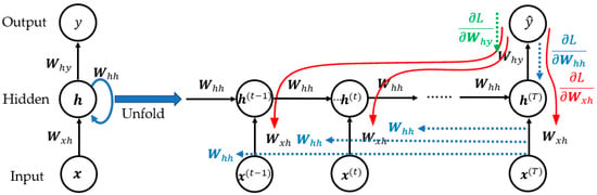
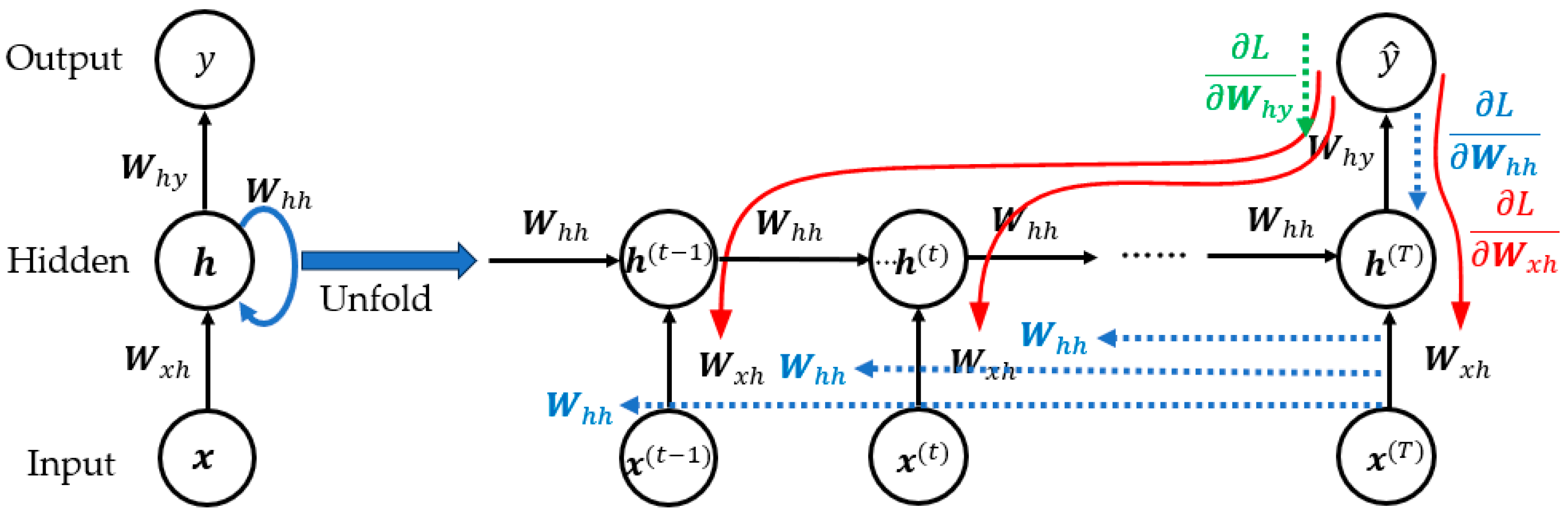
The RNNs are a neural network architecture designed for modeling sequential and time-series data. The core mechanism of the RNNs lies in its ability to capture temporal dependencies through recursive connections in the hidden layers [31]. As illustrated in the N-to-1 architecture shown in Figure 1, the RNNs introduce cyclical connections along the time dimension, establishing a dynamic relationship between the current hidden state and the previous hidden state . This structure allows the model to incorporate both the current input and the previous time step, thereby retaining contextual information and effectively model dynamic features that evolve over time [32].
Figure 1.
N-to-1 architecture diagram of recurrent neural network.
As depicted in Figure 1, the propagation mechanism of RNNs involves two primary processes: forward propagation of the input sequence (black arrows) and backward propagation of the loss gradients with respect to the network parameters (red, green, and blue arrows). Compared with BPNN, RNNs effectively capture long-sequence dependencies through parameter sharing across time steps. The mathematical formulation is given as follows:
The input sequence is , where , denotes the feature dimension, and is the number of time steps. The corresponding hidden layer neurons are , with , and denotes the number of hidden units. The target class label is , where .
(1) Forward propagation: The input sequence is fed into the network sequentially in chronological order. At each time step , the hidden state is a function of the current input and the previous hidden state . The update expression for the hidden layer is:
In Equation (1), is the input-to-hidden layer at time , is the weight matrix from the input layer to the hidden layer, is the recurrent weight matrix between successive hidden states, is the bias vector of the hidden layer, is the output of the hidden layer at time , and is the activation function, typically defined as:
The hidden state at the final time step is then linearly transformed to yield the input of the output layer:
In Equation (3), denotes the weight matrix of the output layer, is the output bias term, and is the input to the output layer at the final time step. For binary classification, this value is mapped to a probability using the sigmoid function:
In Equation (4), represents the posterior probability that a sample belongs to the positive class given its feature vector. A decision threshold is set as , and the classification decision function is defined as:
In this manner, the RNNs recursively process the input sequence, compute the hidden states, and apply a sigmoid transformation at the final time step to produce the classification result.
(2) Backpropagation through time (BPTT): The backward pass employs the BPTT algorithm to compute gradients. By unfolding the RNNs along the time dimension, it is transformed into an equivalent feedforward network, and the gradients of the loss function with respect to the parameters are computed using the chain rule. For binary classification, the commonly used loss function is the binary cross-entropy:
In backpropagation, the error signal at each neuron is defined as the partial derivative of the loss function with respect to its input. For the output layer, the error term is given by . The gradients of the loss function with respect to the output layer weight and the bias term are:
The error term of the hidden layer is denoted as at the final step. For an intermediate time step , the error term is backpropagated to the current hidden layer through both the next hidden state and the output layer. According to the chain rule, the recursive computation of the hidden-layer error at step is:
These recursive calculations of the hidden states across time steps introduce temporal dependencies into the weight matrices and . For the recurrent weight matrix , which maps to the hidden layer, its gradient must be accumulated across all time steps via the corresponding error terms. Thus, the total gradient is expressed as:
Similarly, for the input-to-hidden weight matrix , which maps at time step to the hidden layer , its gradient depends on both the current input and the error term , and the overall gradient is obtained by summing contributions across time steps:
The gradient with respect to the hidden layer bias term is obtained in the same way: .
By combining the above results, the parameter update rules of the RNNs are:
In Equation (11), denotes the learning rate.
Through BPTT, the RNNs recursively compute error terms and parameter gradients at each time step, which are updated iteratively using stochastic gradient descent (SGD), thereby completing the temporal backpropagation process.
3. Data Processing and Indicator Selection
3.1. Data Source and Sample Selection
To enhance the effectiveness of financial crisis prediction for listed companies, this study uses the “Special Treatment” (ST) status as a proxy indicator of financial crisis. Compared with lagging indicators such as bankruptcy or default, the ST designation reflects earlier regulatory intervention and thus provides earlier signals, higher risk sensitivity, and greater practical feasibility for early warning purposes [33,34].
The ST classification information and firm-level financial and non-financial data are obtained from the China Stock Market & Accounting Research (CSMAR) database, which is a widely used and authoritative data source in empirical studies on Chinese capital markets. Specifically, ST status is identified based on the “Special Treatment Changes” dataset released by the China Securities Regulatory Commission (CSRC) and archived in CSMAR. Financial indicators, including balance sheet, income statement, and cash flow statement variables, are extracted from the CSMAR financial statements database. Non-financial indicators, such as corporate governance characteristics and ownership structure variables, are collected from the corresponding governance and firm profile modules in CSMAR.
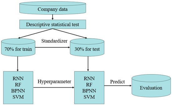
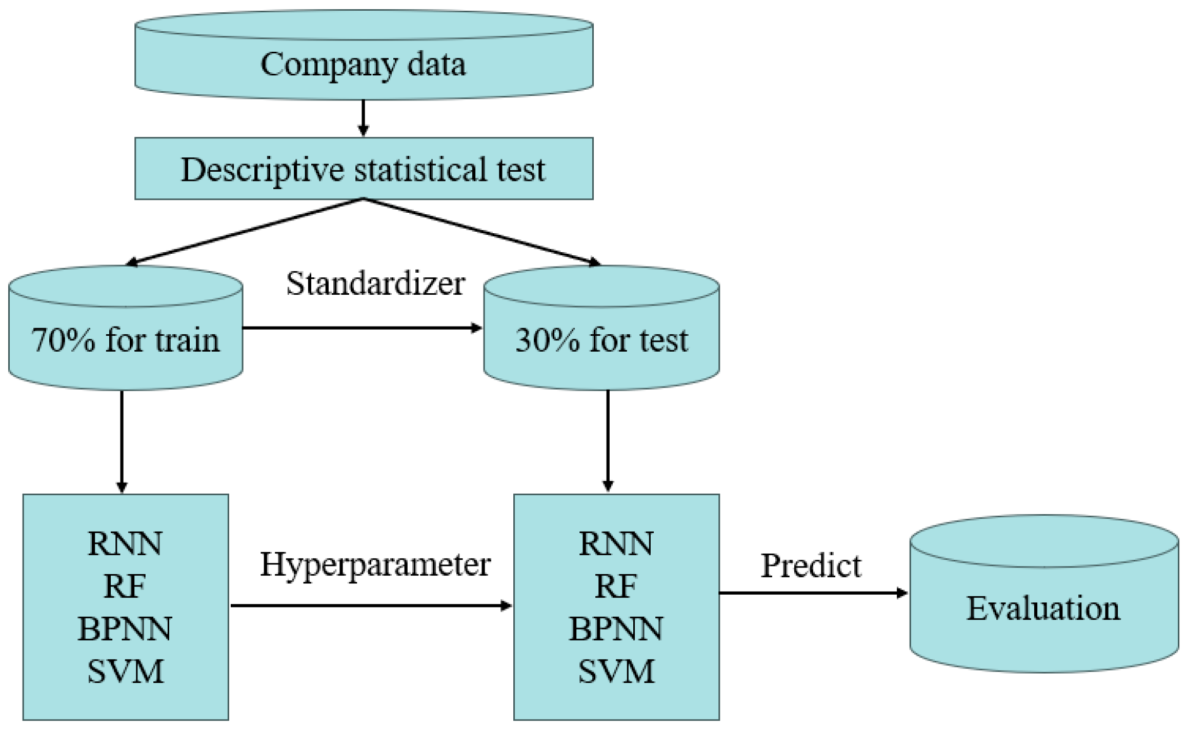
For sample construction, the year 2024 is selected as the base year. Companies classified as ST in 2024 constitute the crisis group, and their financial and non-financial information from 2019 to 2023 is used to construct multi-period input sequences for model training. After missing value processing, 152 ST firms are retained as valid positive samples. To address class imbalance and control for industry-specific effects, a one-to-one matching strategy is applied. Non-ST firms are selected from the same CSRC industry classification and matched by firm size, measured by total assets within a ±10% range. As a result, a balanced dataset comprising 304 listed companies (152 ST and 152 non-ST) is constructed for subsequent model training and evaluation. The overall experimental procedure is illustrated in Figure 2.
Figure 2.
Model construction process.
All the data processing, model construction and result visualization in this study were implemented using Python 3.12. This software is developed and maintained by the Python Software Foundation (PSF), with its official address at Beaverton, OR, USA.
3.2. Selection of Financial Indicators
Based on the research objective of predicting financial crises, this study systematically examines the characteristics of financial risk and, drawing on existing literature on early warning indicator selection, incorporates four additional indicators—operating cost ratio, capital intensity, proportion of independent directors, and total number of companies in the industry—to constructs an evaluation framework comprising 32 risk indicators [35,36,37]. These indicators are divided into two categories:financial and non-financial. Among the financial indicators, the operating cost ratio reflects the stability of a compa-ny’s cost control and profitability, while the capital intensity measures the efficiency of the company’s asset utilization and operational flexibility. Among the non-financial indica-tors, the proportion of independent directors reflects the governance level of the company, and the total number of companies in this industry reflects the competition level and market environment of the industry in which the company is located. By incorporating these indicators into the assessment framework, this framework can provide a more sys-tematic and comprehensive early warning for the financial crisis. And the financial indicators are further organized into five dimensions: solvency, profitability, operational efficiency, growth potential, and cash flow capacity. Table 2 summarizes the complete indicator system.
Table 2.
Financial index system.
3.3. Descriptive Statistical Analysis
To provide an overall understanding of the sample characteristics, descriptive statistical analyses were conducted for all variables included in the study. The statistics were computed separately for distressed (ST) and non-distressed (non-ST) firms. Due to space limitations, representative descriptive statistics are reported in Table 3 and Table 4, while the complete set of results is presented in Table A1 and Table A2 in Appendix A.
Table 3.
Descriptive statistics of some indicators for non-ST enterprises.
Table 4.
Descriptive statistics of some indicators for ST enterprises.
The descriptive statistics reported in Table 3 and Table 4 provide an initial overview of the financial characteristics of crisis and non-crisis enterprises. Overall, noticeable differences can be observed across multiple indicators, suggesting potential heterogeneity between the two groups. To formally examine whether these observed differences are statistically significant, independent-sample t-tests are conducted for all selected indicators. The results show that only five indicators—namely, the revenue growth rate, the operating index, the proportion of independent directors, the net cash flow from operating activities, and the net cash flow from investment activities—do not exhibit significant differences at the 5% significance level, whereas the remaining indicators differ significantly between crisis and non-crisis enterprises. The detailed t-test results are reported in Table A3 in Appendix A.
Given that some variables did not conform to a normal distribution, we further adopted the non-parametric Mann–Whitney U test as a robustness test. The results showed that all other indicators except for the proportion of independent directors had statistically significant differences between crisis enterprises and non-crisis enterprises. The complete U-test results can be found in Table A4 in Appendix A.
Overall, the consistency between the parametric test results and the non-parametric test results indicates that the selected sample has significant and reliable group differences, which provides support for the validity of the constructed indicator system.
3.4. Data Processing
This study adopts a dual-level grouping strategy based on firms and years, that is, the data are grouped by firm and year, where each firm includes five years of annual data and 32 feature indicators. Then, data quality screening is conducted on the original observational samples. The specific processing workflow is as follows:
First, companies with more than 25% missing financial data across the reported years are excluded to reduce noise. For the remaining firms, missing values for each indicator are imputed using the firm-specific cross-period mean, preserving data continuity while minimizing imputation bias. Second, the preprocessed dataset is randomly split into training and test sets at a 7:3 ratio, where the training set comprises 104 ST companies and 108 non-ST companies, and the test set consists of 48 ST companies and 44 non-ST companies. Third, to mitigate convergence issues caused by heterogeneous feature scales, all input variables are standardized using z-score normalization, defined as follows:
In Equation (12), denotes the standardized value of sample on feature dimension. Specifically, is the original value, is the mean of feature in the training set, and is the corresponding standard deviation. For the test set, the normalization is performed using the parameters and computed from the training set, in order to avoid information leakage and maintain consistency in the feature space. The data processing involved in the above process and the related scripts are all stored in the Supplementary Materials (Supplementary Folder S1).
3.4.1. Single-Period Data Processing
For single-year cross-sectional prediction, the z-score standardized values of 32 financial indicators are used to construct the input feature matrix, denoted as . Here, represents the column vector of feature , and is the number of enterprises ( for the training set and for the test set). The label variable is defined as the enterprise classification in 2024, where . The resulting sample matrix, composed of input features and label variables, is expressed as follows:
In Equation (13), represents the financial feature matrix of all enterprises in year .
3.4.2. Multi-Period Data Processing
Since RF, SVM, and BPNN are not inherently designed for sequential data, this study converts historical observations from 2019 to 2023 into static feature representations. Specifically, the original feature vector with 32 dimensions for each year is concatenated across a 5-year window, yielding a 160-dimensional composite feature vector as the input for each enterprise. The label variable is defined as the 2024 classification of the corresponding company. The resulting sample matrix is structured as follows:
In Equation (14), denotes the standardized vector with 32 dimensions for the enterprise in year , where , and . Here, is the number of enterprises ( for the training set and for the test set). The label denotes the class of enterprise in 2024.
In contrast, the RNNs utilize their recurrent hidden state mechanism to capture temporal dependencies without requiring prior flattening of sequential data as specified in Equation (14). In RNNs, for each enterprise, the input consists of 32 feature indicators observed over five consecutive years, which can be structured as a sequence of length 5 with 32 features at each time step, as follows:
In Equation (15), represents the standardized value of feature of an enterprise in year , where . All enterprise samples are stacked to form an input tensor with three dimensions, where n is the number of enterprises ( for the training set and for the test set), 5 is the number of time steps, and 32 is the number of features. The input sample set of the model is composed of the input tensor and the class label vector , that is, . Each element in corresponds to the classification label of an enterprise in 2024, which serves as the prediction target for the model based on its entire historical sequence.
3.5. Hyperparameter Settings
Hyperparameters in this experiment were selected based on commonly adopted empirical ranges in the literature and preliminary validation experiments. Rather than pursuing dataset-specific optimal tuning, this study prioritizes structural consistency and controlled model complexity to ensure fair comparison across models and years. The hyperparameter configurations of all benchmark models are summarized in Table 5.
Table 5.
Hyperparameter settings of benchmark models.
3.6. Evaluation Metrics
In Table 6, the confusion matrix is composed of four fundamental components: True Positive (TP), True Negative (TN), False Positive (FP), and False Negative (FN). Specifically, TP denotes the number of ST companies correctly identified as ST; FP denotes the number of non-ST companies misclassified as ST; TN denotes the number of non-ST companies correctly identified as non-ST; and FN denotes the number of ST companies misclassified as non-ST.
Table 6.
Confusion matrix.
This study adopts five widely used performance metrics to evaluate model performance: accuracy, precision, recall, F1 score, and AUC. Accuracy is the proportion of correctly classified samples. Precision is the proportion of predicted ST samples that are actually ST. Recall is the proportion of actual ST samples correctly identified. The F1 score is the harmonic mean of precision and recall, reflecting the trade-off between the two. AUC is the area under the ROC curve, defined by the True Positive Rate (TPR, equivalent to recall) against the False Positive Rate (FPR). For all metrics, higher values indicate better classification performance. The corresponding formulas are provided in Equations (16)–(20).
4. Model Training and Result Analysis
To evaluate the adaptability and predictive performance of different algorithms on static and time-series data, this section conducts a comparative analysis of RF, SVM, BPNN, and RNNs under two experimental scenarios. The experimental design is structured along two dimensions. First, a horizontal comparison is performed using five years of single-period data to assess each model’s accuracy, stability, and sensitivity to data fluctuations in static prediction. Second, a vertical comparison is carried out on time-series data, where multiple evaluation metrics are applied to examine the ability of the four models to capture temporal evolution patterns during the modeling process.
4.1. Single-Period Data Modeling and Prediction
Following the procedure described in Section 3.4.1, data from each year between 2019 and 2023 were standardized to construct five year-specific static datasets. RF, SVM, BPNN, and RNNs were trained and evaluated on each dataset separately, and the corresponding predictive performance results are reported in Table 7. The complete configuration details and implementation scripts are all included in the Supplementary Materials (Supplementary Folder S2).
Table 7.
Model prediction results based on independent cross-sectional data from 2019 to 2023.
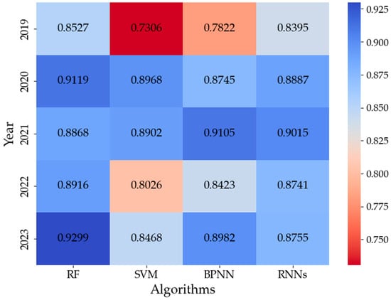
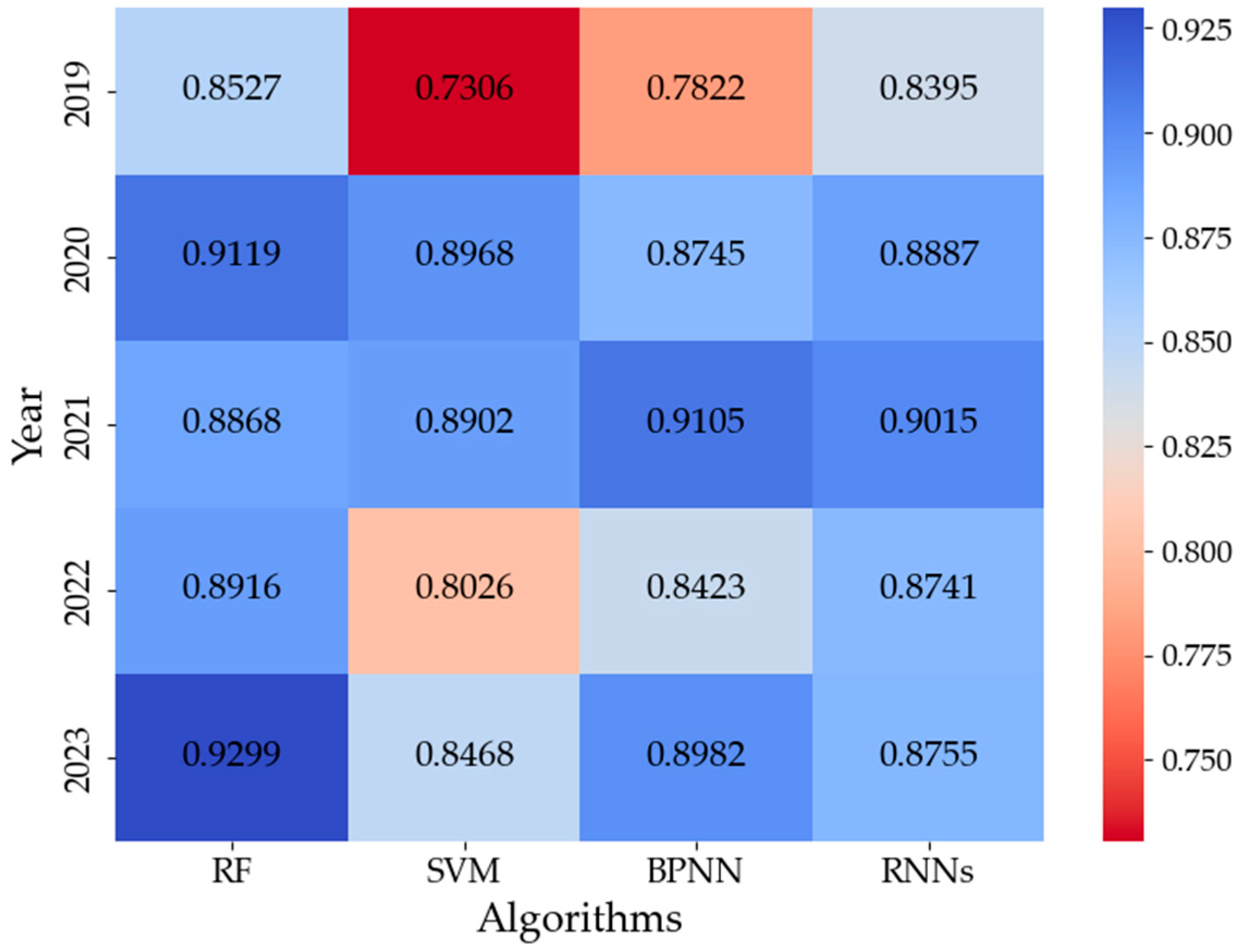
To illustrate the year-to-year variation in AUC for each algorithm, we constructed an AUC heatmap, as shown in Figure 3. In this visualization, darker shades of blue represent higher AUC values.
Figure 3.
Heatmap of AUC for four models across five years (2019–2023).
Taken together, the results from Table 7 and Figure 3 reveal the distinct characteristics of the four models in cross-sectional prediction within single-period experiments. The RF demonstrated excellent overall predictive performance for independent cross-sectional data in all years from 2019 to 2023. Especially after 2020, RF maintained a relatively stable and high level of classification accuracy and recall rate. More importantly, the AUC value of RF remained above 0.85 in all years and reached a peak of 0.9299 in 2023, indicating its excellent discrimination ability and robust ranking performance. This demonstrates the effectiveness of RF in capturing the complex nonlinear relationships among financial indicators and its ability to withstand the annual fluctuations in data distribution.
The SVM performed quite well in 2020 and 2021. The accuracy rates reached 0.8370 and 0.8587 respectively, and the recall rates both reached 0.8750. The AUC value in 2020 reached 0.8968, which was comparable to the results reported in the enterprise bankruptcy research reports of References [38,39]. However, its AUC value showed significant inter-period variability over the five years, ranging from 0.7306 to 0.8968, indicating that it is more sensitive to the changes in the data distribution of different years. This has limited its applicability in cross-sectional settings for the purpose of providing continuous and reliable early warning of financial risks.
The BPNN demonstrated strong predictive capabilities in 2020 and 2021, achieving high accuracy (0.8478 and 0.8913) and F1 scores (0.8627 and 0.8958). Moreover, its AUC value reached 0.9105 in 2021. These results indicate that BPNN is effective in modeling the nonlinear interactions among financial variables within a single-period framework. However, its overall performance was relatively weak in 2019 and 2022. This suggests that although BPNN can achieve high prediction accuracy under good data conditions, compared to the random forest method which is more ensemble-based, its generalization ability on different annual samples has certain limitations.
The RNNs did not show significant performance advantages when applied to independent cross-sectional data. Although the AUC value of RNNs remained at a high level, their overall performance in terms of accuracy, precision, recall, and F1 score was still inferior to the random forest and BPNN after 2020. This may be due to the RNNs’ reliance on temporal dependencies, which cannot be fully leveraged in static, cross-sectional datasets without sequential structure.
4.2. Multi-Period Data Modeling and Prediction
4.2.1. Multi-Period Data Prediction Results
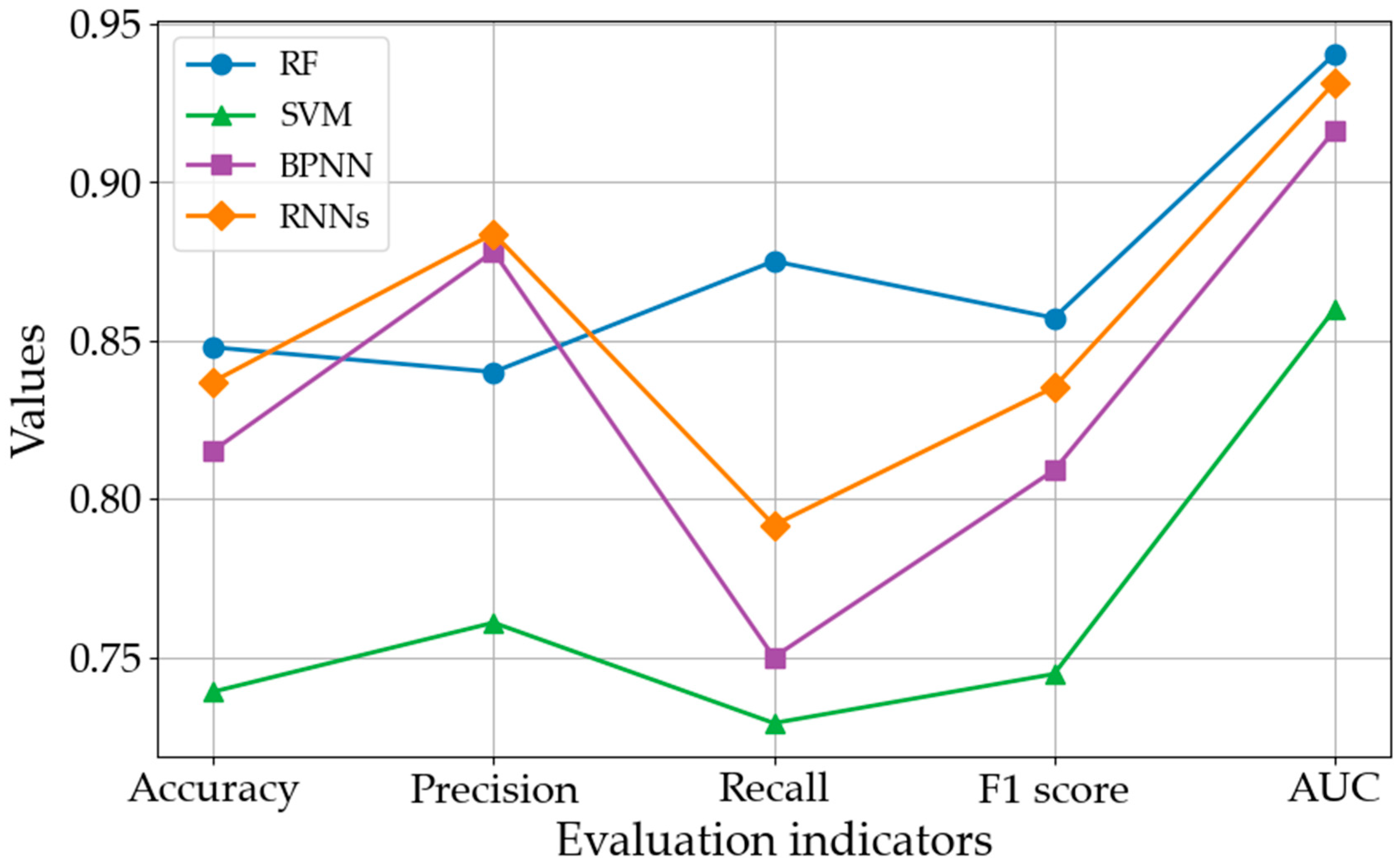
Based on the data processing procedures described in Section 3.4.2, this section constructs a framework for comparing multiple models. For RF, SVM, and BPNN, the input samples are generated by concatenating five years of historical financial indicators into an expanded feature set. In contrast, the RNNs utilize continuous time-series data from 2019 to 2023, along with the corresponding company classification labels, enabling the model to directly capture temporal dependencies through its recurrent structure. In addition, time-series data from 2021 to 2023 are also employed to construct a shorter multi-period setting for comparison. The relevant configuration of the model and the implementation script are all included in the Supplementary Materials (Supplementary Folder S3).
The predictive performance of all models is evaluated under both three-year and five-year observation windows using a comprehensive set of evaluation metrics. Beyond traditional classification indicators, this study further incorporates log loss and Brier score to assess the reliability and calibration quality of probabilistic predictions.
Specifically, Log Loss assigns higher penalties to high-confidence incorrect predictions, thereby capturing deviations in the model’s probability outputs and its sensitivity to overconfident misclassification. In contrast, the Brier score evaluates the overall probability calibration level by measuring the mean squared error between predicted probabilities and observed outcomes.
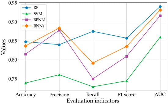
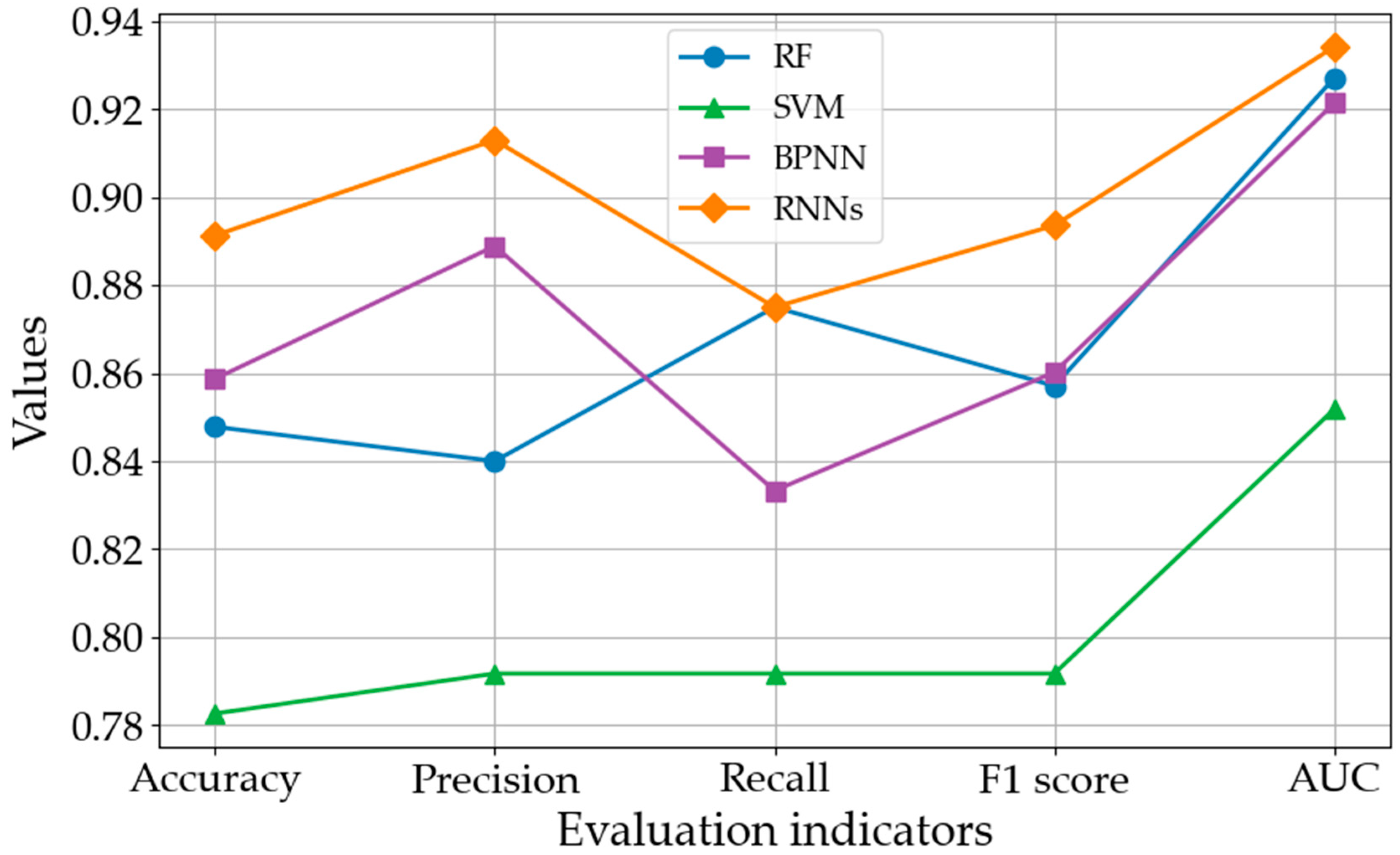
The detailed numerical results are summarized in Table 8 and Table 9, while the corresponding comparisons across different evaluation metrics are illustrated in Figure 4 and Figure 5.
Table 8.
Comparison of model evaluation results based on multi-period data from 2021 to 2023.
Table 9.
Comparison of model evaluation results based on multi-period data from 2019 to 2023.
Figure 4.
Performance comparison based on 2021–2023 multi-period data.
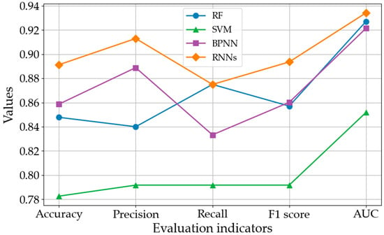
Figure 5.
Performance comparison based on 2019–2023 multi-period data.
As shown in Table 8 and Figure 4, under the three-year observation window, the Random Forest model exhibits relatively strong performance, achieving high levels of accuracy (0.8478), recall (0.8750), and AUC (0.9403). This indicates that the Random Forest model is effective in capturing short-term nonlinear relationships through static aggregation of multi-period financial indicators. By contrast, under this shorter temporal horizon, the RNN-based model does not yet demonstrate a clear advantage across all conventional classification metrics.
Nevertheless, the RNN-based model begins to show advantages in terms of probabilistic prediction. Specifically, it achieves the highest precision (0.8837), while its substantially lower log loss (0.3451) suggests a reduced tendency toward overconfident misclassification. In addition, the lower Brier score (0.1037) further indicates improved calibration consistency between the predicted risk probabilities and the observed outcomes. Taken together, these results suggest that the advantages of RNNs start to emerge under short multi-period settings; however, the limited temporal depth may constrain the model’s ability to fully exploit long-term dependency structures.
A direct comparison between Table 8 (2021–2023) and Table 9 (2019–2023) indicates that extending the observation window leads to more stable and reliable predictive performance across all models, particularly in probability-based metrics. When the window is extended from three to five years, both log loss and Brier score decrease substantially for all models. Specifically, log loss is reduced by approximately 0.2% to 93%, indicating that models trained over a longer temporal horizon are less likely to assign excessively high confidence to incorrect predictions, thereby mitigating the risk of severe misclassification caused by extreme probability estimates. Meanwhile, the Brier score declines by approximately −1% to 42%, reflecting an improvement in overall probability calibration, such that the predicted crisis probabilities are more closely aligned with the observed distress outcomes. Notably, the RNN-based model consistently achieves the lowest log loss and Brier score in both settings, while its relative advantage over RF and BPNN becomes more stable under the longer window. These results suggest that incorporating a longer temporal horizon enables the model to better capture the accumulation, persistence, and delayed manifestation of financial risk, thereby enhancing the practical reliability of early warning signals.
Under the five-year framework, the RNN-based model demonstrates the strongest overall predictive performance on corporate time-series financial data. Specifically, RNNs achieve the highest accuracy (0.8913), F1 score (0.8936) and AUC (0.9342) among all models. Compared with the benchmark methods, the RNNs improve accuracy by approximately 14% relative to SVM and 5% relative to RF, while the F1 score increases by about 13% and 4%, respectively. In terms of ranking performance, the AUC of RNNs exceeds that of SVM by roughly 10%, indicating a markedly stronger discriminative capability under multi-period settings.
Beyond these overall performance gains, the RNN-based model also exhibits clear advantages in terms of error-type distribution. RNNs achieve the highest precision (0.9130) among all models, representing improvements of approximately 15%, 9%, and 3% over SVM, RF and BPNN, respectively, while maintaining a recall level of 0.8750 that is comparable to RF and higher than those of SVM and BPNN by about 11% and 5%. This indicates that the superior performance of RNNs is not achieved at the expense of increased false negatives, but rather through a more balanced trade-off between precision and recall. These results further highlight the effectiveness of recurrent architectures in capturing temporal dependencies and nonlinear dynamics inherent in corporate financial risk evolution.
By comparison, the benchmark models also demonstrate relatively strong but differentiated performance under the five-year framework. Among them, BPNN performs competitively, achieving a precision of 0.8889, an F1 score of 0.8602 and an AUC of 0.9214, reflecting its ability to approximate complex nonlinear mappings through activation functions. RF shows robust performance, with recall (0.8750) and AUC (0.9271) comparable to those of the RNN-based model, highlighting its strong generalization capability and suitability for applications where interpretability is desirable. In contrast, SVM exhibits relatively weaker performance, with an accuracy of 0.7826 and an AUC of 0.8518, suggesting limitations in capturing high-dimensional nonlinear feature interactions in multi-period financial data.
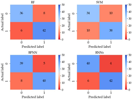
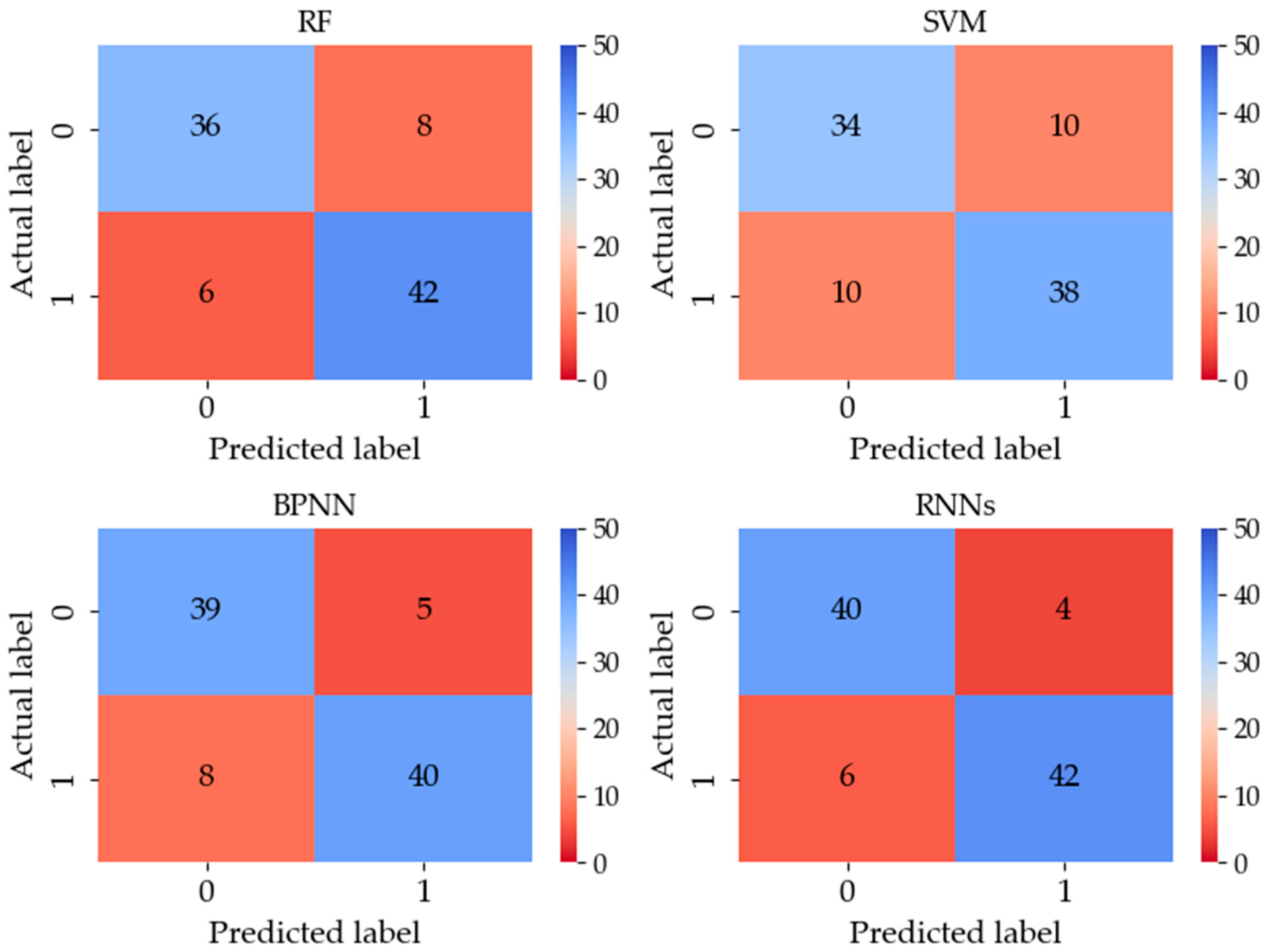
To further analyze model performance, confusion matrix heatmaps are employed to visualize the correspondence between predicted and actual labels. As shown in Figure 6, darker colors along the main diagonal indicate a higher number of correctly classified samples, whereas off-diagonal cells represent misclassification patterns across classes.
Figure 6.
Confusion matrix heatmap of four models based on multi-period data from 2019 to 2023.
It can be observed that the RNNs achieve a well-balanced performance in distinguishing between ST and non-ST companies, attaining the highest values of both true positives (TP) and true negatives (TN), while maintaining the lowest false positive rate (FPR) and false negative rate (FNR). These results indicate robust and stable class recognition capability.
Although the RF model demonstrates strong identification ability for ST companies, it exhibits a relatively high misclassification rate for non-ST companies, with an FPR of 14.3%. Such a skewed prediction tendency may cause unnecessary regulatory interventions and increased compliance costs in practice, thereby limiting its suitability for fine-grained management applications.
The BPNN also achieves a reasonable balance between positive and negative class predictions. However, its inability to explicitly capture temporal dependencies constrains its effectiveness in dynamic financial data environments, leading to lower overall accuracy compared to the RNNs.
The SVM, by contrast, shows a relatively high number of misclassified samples, as indicated by the more pronounced off-diagonal color blocks in the heatmap. This pattern suggests deficiencies in feature representation and highlights the model’s limited capacity to capture the complex temporal and nonlinear characteristics of financial data.
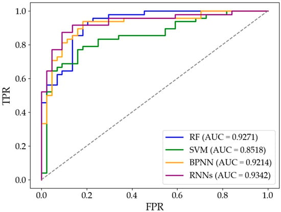
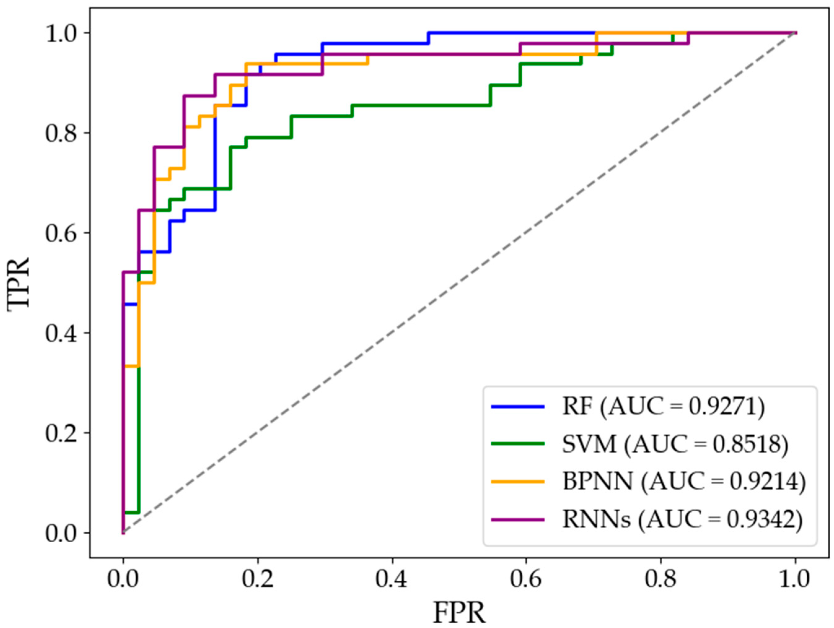
The Receiver Operating Characteristic (ROC) curve provides an additional perspective for evaluating classifier performance. In general, the closer the curve lies to the top-left corner, the stronger the classifier’s ability to maximize true positive rate (TPR) while minimizing false positive rate (FPR) across varying thresholds. Figure 7 presents the ROC curves of the four models in the context of financial crisis prediction.
Figure 7.
ROC curves of four models based on multi-period data from 2019 to 2023.
It can be observed that the ROC curve of the RNNs lies closest to the upper-left corner, indicating superior classification performance. Notably, within the FPR range below 0.1, the TPR exceeds 80%, suggesting that even under stringent control of false positives, the model retains strong crisis detection capability. This characteristic makes the RNNs well-suited for scenarios requiring high detection accuracy with minimal tolerance for false alarms.
The ROC curve of the RF shows pronounced slope variation, particularly in the FPR range of 0.0 to 0.2, where the curve rises steeply. This indicates that the model is highly sensitive to threshold adjustments, which can be advantageous in decision-making contexts where the trade-off between false positives and false negatives must be tailored to risk tolerance or policy requirements.
In contrast, the ROC curve of the SVM deviates considerably from the upper-left corner, with only gradual increases in TPR as FPR rises, reflecting weaker overall discriminative ability. Although the BPNN achieves better results than the SVM, its rate of TPR improvement in the low-FPR region and the overall curve trajectory remain less competitive than those of the RNNs and RF.
In summary, the RNNs demonstrate the strongest performance in tasks involving time-series data, highlighting their effectiveness in capturing complex and dynamically evolving financial risks. Meanwhile, the RF and BPNN also show solid predictive capabilities and may serve as viable alternatives depending on specific application requirements.
4.2.2. Statistical Validation of Model Comparisons
To rigorously examine whether the observed performance differences are statistically meaningful, multiple complementary statistical tests are conducted.
First, the McNemar test is applied to compare the classification accuracy of the RNNs with each benchmark model. The results for the overall sample and the crisis (ST) subsample are reported in Table 10 and Table 11, respectively.
Table 10.
McNemar test results on overall sample: RNNs vs. benchmark models.
Table 11.
McNemar test results on crisis companies: RNNs vs. benchmark models.
The results show that none of the pairwise comparisons reach statistical significance at the 5% level for either the overall sample or the crisis (ST) subsamples. These findings indicate that the RNNs achieve non-inferior classification performance relative to RF, SVM, and BPNN, rather than statistically dominating them in terms of accuracy.
Second, the Deboer-Marinov pair test was used to further compare the logarithmic loss of the model, in order to evaluate the quality of the model’s probability predictions. The results are shown in Table 12.
Table 12.
Paired log-loss comparison (RNNs vs. baselines).
It can be seen that at the significance level of 0.05, RNN did not reject the null hy-pothesis of equal prediction accuracy compared to the baseline model, but the estimated loss differences always indicated that the recurrent neural network had a significant ad-vantage over all the baseline models. This pattern suggests a systematic, albeit moderate, advantage in probability estimation.
Third, a bootstrap resampling procedure is employed to assess the robustness and stability of performance differences. The results are shown in Table 13.
Table 13.
Bootstrap confidence intervals for performance differences (RNNs: baseline).
The bootstrap confidence intervals reveal that the RNNs exhibit a statistically stable advantage over the SVM in terms of AUC and probabilistic loss, with confidence intervals excluding zero. In contrast, the confidence intervals for comparisons with RF and BPNN include zero, indicating that while the performance differences consistently favor the RNNs, they are less pronounced under the current sample size.
4.2.3. Feature Importance Analysis
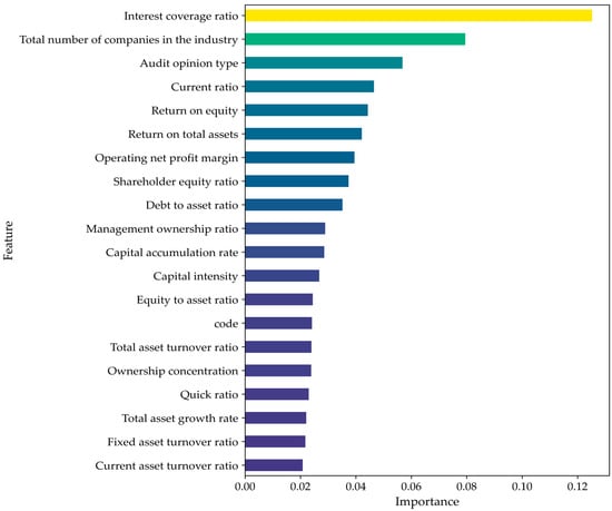
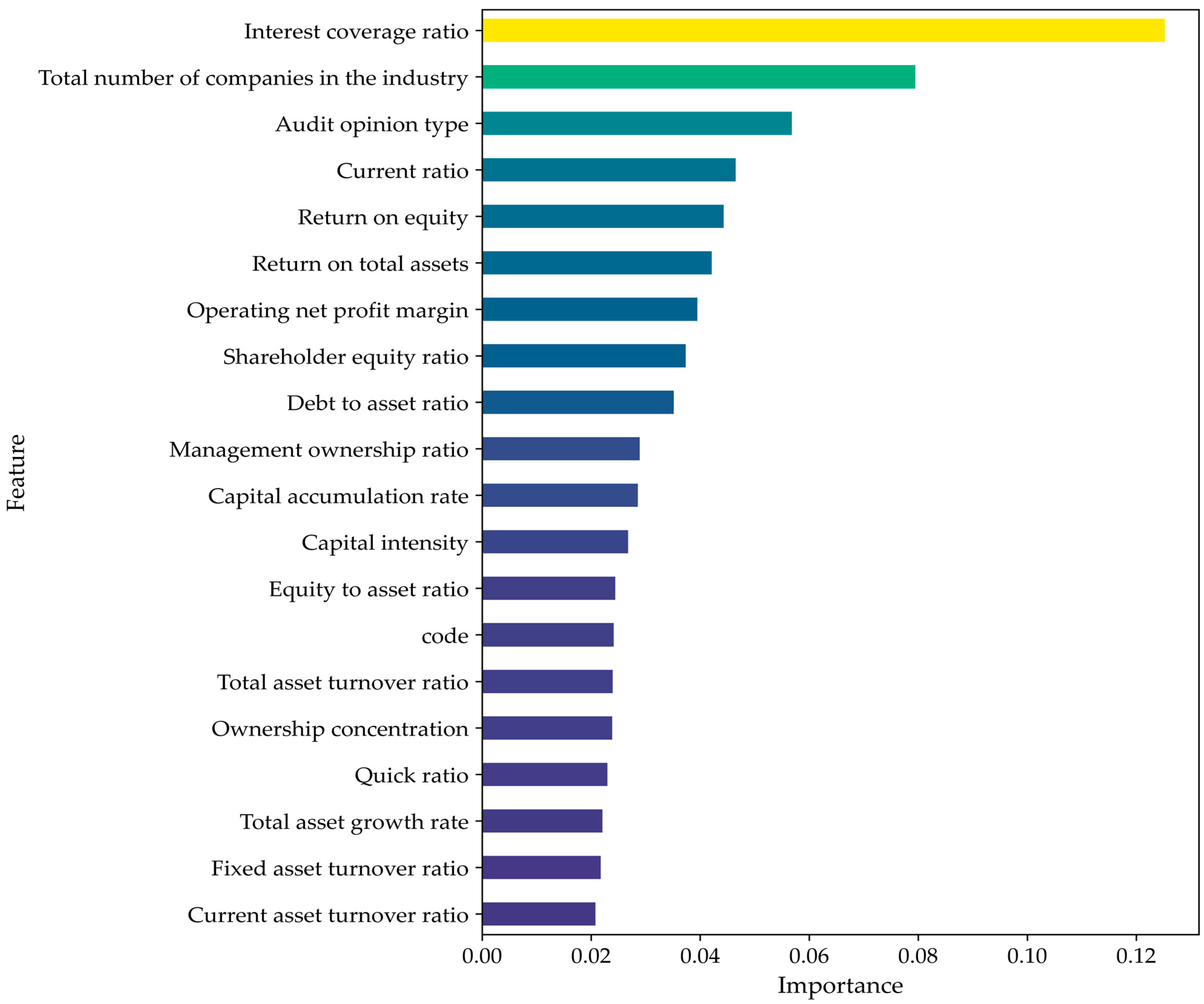
To further assess the economic rationality of the constructed indicator system, a feature importance analysis based on the RF model is conducted, as illustrated in Figure 8.
Figure 8.
Top 20 feature importance scores derived from the Random Forest model, measured by mean decrease in impurity. Colors are only used to distinguish variables; bar length represents variable importance.
Figure 8 shows the importance of the top 20 features. The complete set of indicator results can be found in Figure A1. Among them, the interest coverage ratio is the most important, indicating that the ability of an enterprise to cover interest expenses is the primary factor distinguishing crisis enterprises from non-crisis enterprises. The continuous decline of this indicator usually means tight cash flow and rising leverage pressure, which are typical leading signals of financial distress accumulation and exposure. The total number of companies in the industry ranks second, indicating that the intensity of industry competition has a significant impact on the financial risk of enterprises. Enterprise crises not only stem from internal operating conditions but are also constrained by the external industry environment. The audit opinion type, as an important external governance and information disclosure indicator, also has strong warning value in risk identification. At the same time, the current ratio and return on equity depict the financial stability of enterprises from the perspectives of short-term debt repayment ability and profitability, and their relatively high importance indicates that insufficient liquidity and continuous weakening of profitability are important sources of enterprise financial risk accumulation.
From the overall distribution of the 20 features, the key variables identified by the RF model are mainly concentrated in three dimensions: debt repayment ability, cash flow status, and profitability. This is highly consistent with the economic formation mechanism of enterprise financial crises. The debt and liquidity indicators occupied a dominant position in the importance ranking, indicating that enterprise crises often first manifest as the concentrated emergence of debt pressure and liquidity constraints; the profitability indicators also had a relatively high weight, reflecting that financial crises usually result from the continuous decline in profitability rather than short-term shocks. In contrast, the importance of growth, operational efficiency, and governance indicators was relatively low, but they still provided supplementary information for the long-term development characteristics and institutional environment of the enterprise.
Overall, the feature importance results demonstrate that the predictive performance of the proposed framework is driven by economically meaningful indicator categories rather than by isolated variables. Moreover, the dominance of cash flow, profitability, and solvency indicators—whose deterioration typically unfolds gradually over time—provides further justification for RNNs to capture the dynamic evolution and cumulative nature of corporate financial risk.
5. Conclusions
This study provides a systematic evaluation of the predictive performance of RF, SVM, BPNN, and RNN-based models for financial crisis early warning among Chinese A-share listed companies over the period 2019–2023. The main conclusions are as follows:
First, the empirical results confirm that financial crisis prediction performance is influenced by the data structure adopted for modeling. In single-period, cross-sectional settings, RF and BPNN exhibit robust and competitive performance, achieving relatively stable accuracy and F1 score across different years. However, when multi-period temporal information is explicitly incorporated, their relative advantages diminish. In contrast, RNN-based models consistently benefit from sequential inputs, achieving improvements of approximately 5–14% in accuracy and 4–13% in F1 score compared with traditional machine learning baselines under the five-year framework. This finding demonstrates the superior capability of recurrent architectures in capturing inter-temporal dependencies and gradual risk accumulation.
Second, under the five-year time-series setting, RNNs achieve the best overall performance across multiple evaluation dimensions. In particular, compared with support vector machines, RNNs increased the AUC value by approximately 10%. Statistical validation using McNemar tests, paired log loss comparisons, and bootstrap confidence intervals indicates that these improvements are systematic but moderate under the current sample size, suggesting stable rather than statistically dominant advantages.
Third, a direct comparison between shorter (three-year) and longer (five-year) temporal windows reveals that extending the observation horizon leads to substantial improvements in probabilistic prediction stability across all models. On the one hand, the pronounced reduction in log loss indicates that models trained on longer time series are better able to suppress overconfident incorrect predictions, thereby reducing the risk of severe misclassification caused by extreme probability estimates. On the other hand, the decline in the Brier score further reflects an improvement in overall probability calibration, such that the predicted crisis probabilities are more closely aligned with the observed distress outcomes. Notably, the RNN-based model consistently achieves the lowest probabilistic loss, highlighting its superior reliability in estimating financial crisis risk.
Overall, this study highlights the importance of aligning model choice and temporal window length with the dynamic characteristics of financial risk evolution. By systematically comparing static, short-horizon, and long-horizon modeling strategies under controlled experimental conditions, the findings demonstrate that incorporating longer-term temporal information can yield quantifiable and stable performance gains in financial crisis prediction. These results provide practical guidance for enterprises and regulators in selecting appropriate early warning frameworks. Future research may further extend this work by exploring adaptive temporal window selection, attention-based mechanisms, or the integration of multi-source heterogeneous data to enhance predictive accuracy and interpretability.
Supplementary Materials
The following supporting information can be downloaded at: https://www.mdpi.com/article/10.3390/math14040657/s1, Folder S1: Financial indicators description and data processing; Folder S2: model prediction of single-year (2019–2023); Folder S3: model prediction of single-year (2019–2023).
Author Contributions
Y.D.: writing—review and editing, data curation; A.R.: validation, supervision. All authors have read and agreed to the published version of the manuscript.
Funding
This work was sponsored by the National Natural Science Foundation of China (Grant No 32160258) and the APC was funded by the National Natural Science Foundation of China (Grant No 32160258).
Data Availability Statement
The original contributions presented in the study are included in the article; further inquiries can be directed to the corresponding author.
Conflicts of Interest
The authors declare no conflicts of interest.
Abbreviations
The following abbreviations are used in this manuscript:
| RF | Random Forest |
| SVM | Support Vector Machine |
| BPNN | Backpropagation Neural Network |
| RNNs | Recurrent Neural Networks |
| AUC | Area Under the ROC Curve |
| ROC | Receiver Operating Characteristic Curve |
Appendix A. Supplementary Tables
Table A1.
Descriptive statistics of all indicators for non-ST enterprises.
Table A2.
Descriptive statistics of all indicators for ST enterprises.
Table A3.
The results of the t-tests for each indicator.
Table A4.
The results of the U-test for the five indicators.
Appendix B. Supplementary Figure
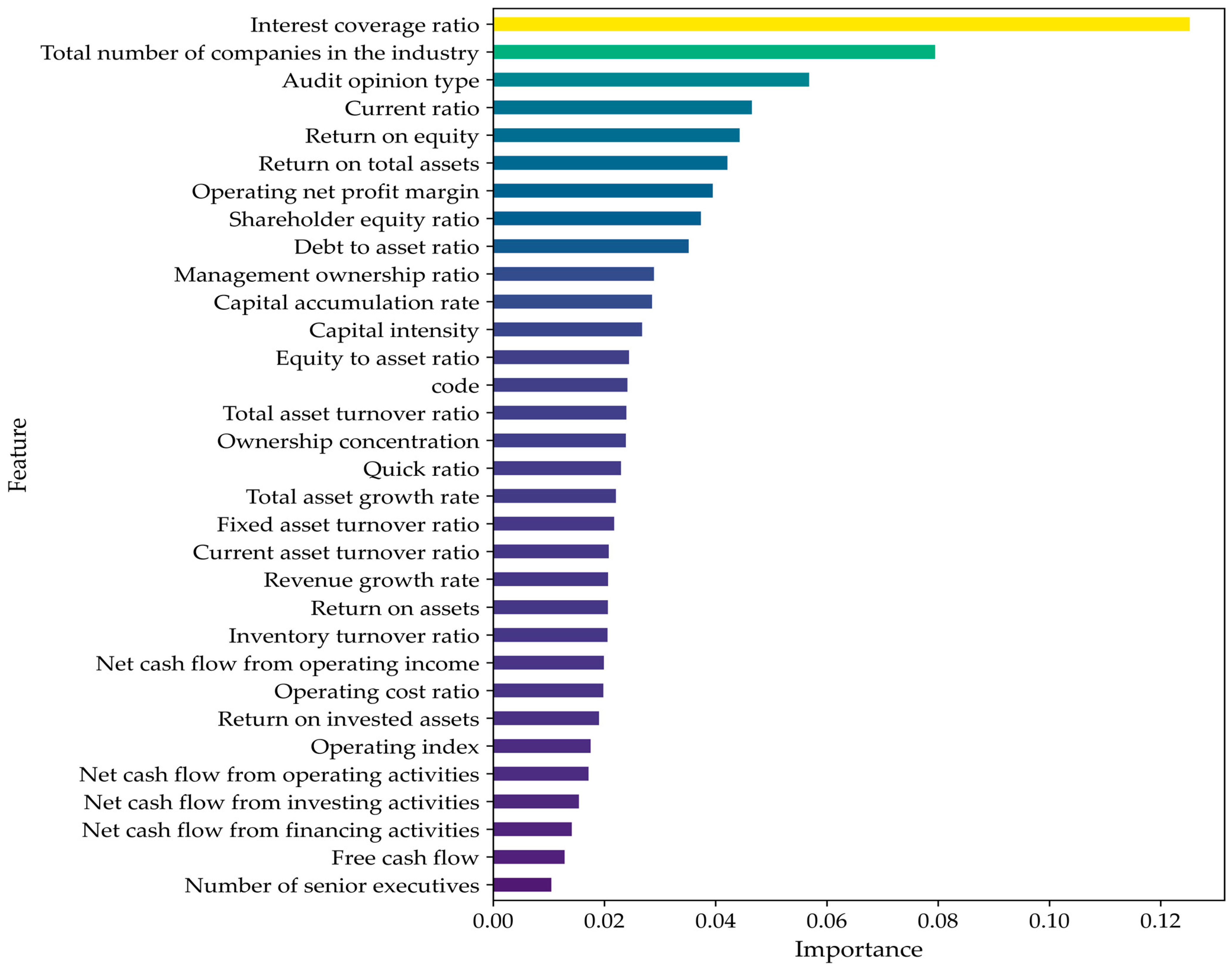
Figure A1.
Thirty-two feature importance scores derived from the Random Forest model, measured by mean decrease in impurity. Colors are only used to distinguish variables; bar length represents variable importance.
References
- Wang, W.; Liu, F. Research on Enterprise Financial Crisis Early Warning Combining Model Based on Historical Data Trend and Single Year Data. In Proceedings of the 3rd IEEE International Conference on Information Technology, Big Data and Artificial Intelligence (ICIBA), Chongqing, China, 26–28 May 2023; IEEE: New York, NY, USA, 2003; pp. 480–484. [Google Scholar] [CrossRef] [Scilit]
- Liang, Y.; Wang, C.; Liu, M. Design of Enterprise Financial Early Warning Model Based on Python. In Proceedings of the 2024 Asia-Pacific Conference on Software Engineering, Social Network Analysis and Intelligent Computing (SSAIC 2024), New Delhi, India, 10–12 January 2024; IEEE: New York, NY, USA, 2024; pp. 727–732. [Google Scholar] [CrossRef] [Scilit]
- Lyu, J.; Xu, H. Design of Modern Enterprise Financial Crisis Warning System Based on Random Forest Algorithm. In Proceedings of the 15th IEEE International Conference on Computational Intelligence and Communication Networks (CICN 2023), Bangkok, Thailand, 22–23 December 2023; IEEE: New York, NY, USA, 2023; pp. 679–684. [Google Scholar] [CrossRef] [Scilit]
- Zhang, C. Research on Financial Crisis Early Warning Optimization of Listed Companies Based on Machine Learning Algorithm. In Proceedings of the 2024 International Conference on Electrical Drives, Power Electronics & Engineering (EDPEE 2024), Athens, Greece, 27–29 February 2024; IEEE: New York, NY, USA, 2024; pp. 743–748. [Google Scholar] [CrossRef] [Scilit]
- Cao, Y.; Shao, Y.; Zhang, H. Study on early warning of E-commerce enterprise financial risk based on deep learning algorithm. Electron. Commer. Res. 2022, 22, 21–36. [Google Scholar] [CrossRef] [Scilit]
- Kivuvo, R.M.; Olweny, T. Financial performance analysis of Kenya’s SACCO sector using the Altman Z-score model of corporate bankruptcy. Int. J. Bus. Soc. Sci. 2014, 5, 34–52. Available online: https://ijbssnet.com/journals/Vol_5_No_9_1_August_2014/4.pdf (accessed on 3 September 2025).
- Bandyopadhyay, A. Predicting probability of default of Indian corporate bonds: Logistic and Z-score model approaches. J. Risk Financ. 2006, 7, 255–272. [Google Scholar] [CrossRef] [Scilit]
- Jaffari, A.A.; Ghafoor, Z. Predicting corporate bankruptcy in Pakistan: A comparative study of multiple discriminant analysis and logistic regression. Res. J. Financ. Account. 2017, 8, 81–100. Available online: https://core.ac.uk/download/pdf/234631944.pdf (accessed on 3 September 2025).
- Zhou, Z.H. Machine Learning; China Minshang Press: Beijing, China, 2016; Available online: https://lib2.buct.edu.cn/bookInfo_01h0228835.html (accessed on 3 September 2025).
- Doğan, S.; Koçak, D.; Atan, M. Financial Distress Prediction Using Support Vector Machines and Logistic Regression. In Advances in Econometrics, Operational Research, Data Science and Actuarial Studies; Springer: Cham, Switzerland, 2022; pp. 429–452. [Google Scholar] [CrossRef] [Scilit]
- Huang, Y. Research on Financial Early Warning Model of Manufacturing Listed Companies Based on Random Forest. Master’s Thesis, East China Jiaotong University, Nanchang, China, 2013. [Google Scholar]
- Zhang, C.; Zhong, H.; Hu, A. Research on Early Warning of Financial Crisis of Listed Companies Based on Random Forest and Time Series. Mob. Inf. Syst. 2022, 1, 1573966. [Google Scholar] [CrossRef] [Scilit]
- Wu, H.M. Financial Risk Early Warning of Manufacturing Enterprises Based on Multiclass Imbalanced Support Vector Machine. Master’s Thesis, Hangzhou Dianzi University, Hangzhou, China, 2024. [Google Scholar]
- Song, X.; Jing, Y.; Qin, X. BP neural network-based early warning model for financial risk of internet financial companies. Cogent Econ. Financ. 2023, 11, 2210362. [Google Scholar] [CrossRef] [Scilit]
- Odom, M.D.; Sharda, R. A neural network model for bankruptcy prediction. In Proceedings of the International Joint Conference on Neural Networks (IJCNN 1990), San Diego, CA, USA, 17–21 June 1990; IEEE: New York, NY, USA, 1990; pp. 163–168. [Google Scholar] [CrossRef] [Scilit]
- Wang, Z.R.; Zeng, F.R. BP neural network-based financial early warning for manufacturing listed companies. Account. Mon. 2008, 2, 56–58. [Google Scholar] [CrossRef]
- Feng, Q.; Chen, H.; Jiang, R. Analysis of early warning of corporate financial risk via deep learning artificial neural network. Microprocess. Microsyst. 2021, 87, 104387. [Google Scholar] [CrossRef] [Scilit]
- Jiang, W.; Wu, X.; Wang, X. Construction and Application of the Financial Early-Warning Model Based on the BP Neural Network. Comput. Intell. Neurosci. 2022, 1, 5108677. [Google Scholar] [CrossRef] [Scilit]
- Kim, H.; Cho, H.; Ryu, D. Corporate default predictions using machine learning: Literature review. Sustainability 2020, 12, 6325. [Google Scholar] [CrossRef] [Scilit]
- Xu, J.; Wang, B.; Sun, X.Y. Risk early warning model of human resource management based on RNN neural network. Comput. Digit. Eng. 2020, 48, 1727–1730. [Google Scholar]
- Liu, C.L.; Lin, B. Prediction of internal control deficiencies of listed companies based on deep learning: New theories and methods. Account. Res. 2024, 6, 119–134. [Google Scholar]
- Kim, H.; Cho, H.; Ryu, D. Corporate Bankruptcy Prediction Using Machine Learning Methodologies with a Focus on Sequential Data. Comput. Econ. 2022, 59, 1231–1249. [Google Scholar] [CrossRef] [Scilit]
- Lombardo, G.; Bertogalli, A.; Consoli, S.; Recupero, D.R. Natural language processing and deep learning for bankruptcy prediction: An end-to-end architecture. IEEE Access 2024, 12, 151075–151091. [Google Scholar] [CrossRef] [Scilit]
- Zhu, Z.; Chen, H.; Qu, Q.; Chung, V. FinCast: A Foundation Model for Financial Time-Series Forecasting. In Proceedings of the 34th ACM International Conference on Information and Knowledge Management, Seoul, Republic of Korea, 10–14 November 2025; Association for Computing Machinery: New York, NY, USA, 2025; pp. 4539–4549. [Google Scholar] [CrossRef] [Scilit]
- Wang, Y.; Xu, Z.; Yao, Y.; Liu, J.; Lin, J. Leveraging Convolutional Neural Network–Transformer Synergy for Predictive Modeling in Risk-Based Applications. arXiv 2024, arXiv:2412.18222. [Google Scholar] [CrossRef] [Scilit]
- Zhou, Y.; Shen, L.; Ballester, L. A two-stage credit scoring model based on random forest: Evidence from Chinese small firms. Int. Rev. Financ. Anal. 2023, 89, 102755. [Google Scholar] [CrossRef] [Scilit]
- Chhajer, P.; Shah, M.; Kshirsagar, A. The applications of artificial neural networks, support vector machines, and long-short term memory for stock market prediction. Decis. Anal. J. 2022, 2, 100015. [Google Scholar] [CrossRef] [Scilit]
- Huang, X.; Guo, F. A kernel fuzzy twin SVM model for early warning systems of extreme financial risks. Int. J. Financ. Econ. 2021, 26, 1459–1468. [Google Scholar] [CrossRef] [Scilit]
- Glorot, X.; Bengio, Y. Understanding the difficulty of training deep feedforward neural networks. In Proceedings of the 13th International Conference on Artificial Intelligence and Statistics (AISTATS 2010), Sardinia, Italy, 13–15 May 2010; PMLR: Cambridge, MA, USA, 2010; pp. 249–256. Available online: https://proceedings.mlr.press/v9/glorot10a.html (accessed on 3 September 2025).
- Zhang, C.; Zhang, J.; Jiang, P. Assessing the risk of green building materials certification using the back-propagation neural network. Environ. Dev. Sustain. 2022, 24, 6925–6952. [Google Scholar] [CrossRef] [Scilit]
- Yan, W.; Song, Y. Intelligent Evaluation and Early Warning of Liquidity Risk of Commercial Banks Based on RNN. Comput. Intell. Neurosci. 2022, 1, 7325798. [Google Scholar] [CrossRef] [Scilit]
- Mienye, I.D.; Swart, T.G.; Obaido, G. Recurrent neural networks: A comprehensive review of architectures, variants, and applications. Information 2024, 15, 517. [Google Scholar] [CrossRef] [Scilit]
- Ostrihoň, F. Evaluating banking crisis predictions in EU and V4 countries. Trendy V Podn. 2020, 10, 64–72. [Google Scholar] [CrossRef] [Scilit]
- Liang, M.; Li, H.X.; Zhang, S.M. Measurement of financial distress based on ST prediction and cross-sectional stock returns. Chin. J. Manag. Sci. 2023, 31, 138–149. [Google Scholar] [CrossRef]
- Zhao, Y.T. Profitability, audit opinion types and financing choices of small and medium-sized enterprises. Account. Commun. 2020, 17, 56–59. [Google Scholar] [CrossRef]
- Tan, J.C.M.; Cao, Q.; Quek, C. FE-RNN: A fuzzy embedded recurrent neural network for improving interpretability of neural networks. Inf. Sci. 2024, 663, 120276. [Google Scholar] [CrossRef] [Scilit]
- Liu, T.; Yang, L. Financial risk early warning model for listed companies using BP neural network and rough set theory. IEEE Access 2024, 12, 27456–27464. [Google Scholar] [CrossRef] [Scilit]
- Xie, C.; Luo, C.; Yu, X. Financial distress prediction based on SVM and MDA methods: The case of Chinese listed companies. Qual. Quant. 2011, 45, 671–686. [Google Scholar] [CrossRef] [Scilit]
- Barboza, F.; Kimura, H.; Altman, E.I. Machine learning models and bankruptcy prediction. Expert Syst. Appl. 2017, 83, 405–417. [Google Scholar] [CrossRef] [Scilit]

Disclaimer/Publisher’s Note: The statements, opinions and data contained in all publications are solely those of the individual author(s) and contributor(s) and not of MDPI and/or the editor(s). MDPI and/or the editor(s) disclaim responsibility for any injury to people or property resulting from any ideas, methods, instructions or products referred to in the content. |
© 2026 by the authors. Licensee MDPI, Basel, Switzerland. This article is an open access article distributed under the terms and conditions of the Creative Commons Attribution (CC BY) license.