


Abstract
In this paper, a coupled-inductor-based interleaved Buck converter is presented. By employing a negatively coupled inductor, the proposed topology reduces magnetic component number and improves dynamic response. Operating in boundary conduction mode (BCM), the proposed converter can achieve zero-voltage switching (ZVS) under a wide voltage and load range. The control strategy is fully digital, allowing the switching frequency to be adaptively adjusted without the need for a zero-crossing detection (ZCD) circuit. Furthermore, an optimal coupling coefficient design is proposed, which minimizes the frequency adjustment range. In addition, the design process for a coupled inductor with an interleaved winding structure is introduced in detail. Finally, a 300 W experimental prototype is built, the experimental results of which demonstrate its effectiveness and feasibility.
MSC:
93C62
1. Introduction
DC/DC converters are widely used in industrial applications such as renewable energy generation and energy storage systems [1,2]. Among them, the Buck and Boost converters are commonly used due to their simple structures [3,4]. As the switching frequency increases, in order to reduce switching losses, ZVS soft switching needs to be adopted. Generally, ZVS can be achieved by adding auxiliary clamping circuits [5,6]. In addition, the zero-voltage transition (ZVT) converter, which can also achieve ZVS operation and effectively reduce switching losses, is implemented [7]. However, the reliability of the system is reduced because of the complexity of the driver circuit and control strategy. In [8,9], the addition of auxiliary capacitors or inductors provides additional current paths to achieve ZVS at a fixed switching frequency. Moreover, adding resonant tanks can allow quasi resonant converters to achieve ZVS operation [10,11]. However, among these types of converters, the presence of additional passive components will still increase hardware costs.
Buck and Boost converters operating in BCM can achieve ZVS without additional auxiliary components [12,13]. ZVS can be achieved by employing a smaller filtering inductor and higher current ripple. However, when the operating conditions change, a higher switching frequency will result in a loss of ZVS, while a lower switching frequency will generate higher circulating current. Therefore, it is necessary to accurately adjust the switching frequency according to different voltages and loads to maintain BCM operation. Adding a zero-crossing detection circuit (ZCD) can achieve BCM operation with good response speed [14,15]. However, ZCD circuits are more sensitive to sampling noise. In addition, high-bandwidth sensors and sampling circuits may also increase hardware costs. In order to simplify hardware circuit design, digital control methods for BCM are studied [16,17,18]. Under digital control, the switching frequency is calculated based on the average value of the voltage and current, effectively reducing the interference of sampling noise.
In addition, compared with a single-phase DC/DC converter, the interleaved DC/DC converter can achieve higher power capacity and lower current ripple [19]. However, two bulky separated inductors will reduce the total power density. In order to improve the power density, the coupled inductor can be adopted to achieve the integration of magnetic components [20,21,22]. Nevertheless, the optimization design of coupling coefficient is rarely discussed. Generally, there are two types of coupled inductor: the positively coupled inductor and negatively coupled inductor. Compared with the positively coupled inductor, the negatively coupled inductor can reduce current ripple and improve dynamic performance [23]. However, in the coupled-inductor-based interleaved DC/DC converter, the inductance parameters and the inductor current modes become more complex. During one switching cycle, the inductor current may have multiple operating modes. Hence, the design of coupled inductors and the control of ZVS operation are more challenging.
On the other hand, under BCM modulation, the switching frequency needs to be adjusted in a wide range at different working voltages. The wide frequency range will bring challenges to the design of magnetic components and driving circuits. Therefore, it is necessary to limit the switching frequency through optimized design.
In this paper, a coupled inductor-based interleaved Buck converter with fully digital control and optimal coupling coefficient is proposed, which has two main advantages as follows:
- (1)
- Compared with traditional interleaved parallel DC/DC converters, the proposed optimal coupling coefficient design minimizes the switching frequency range. This characteristic is advantageous for the design of magnetic components and drive circuits, as it can simultaneously reduce switching and magnetic losses.
- (2)
- The coupled inductor current has multiple stages within one switching cycle. In this regard, a unified equation for adjusting the switching frequency has been proposed, and digital BCM control can be achieved. Furthermore, only the average values of voltage and current need to be sampled.
2. Working Principle and Characteristic Analysis
2.1. Steady State Analysis
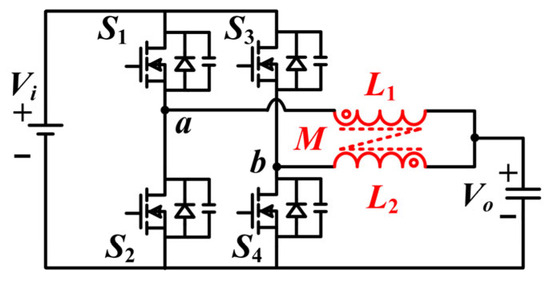
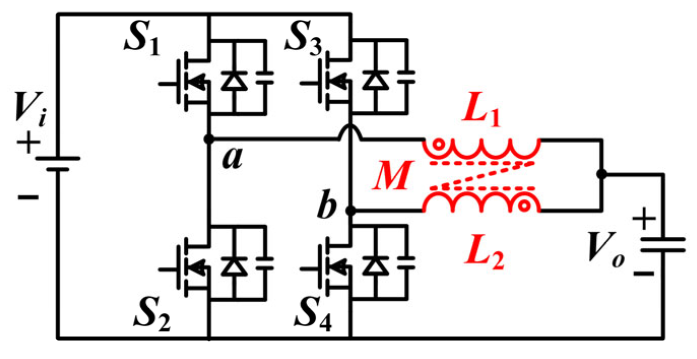
The interleaved Buck converter with negatively coupled inductor is shown in Figure 1. M is mutual inductance. L1 and L2 are self-inductance, and L1 = L2 = L. The input voltage is Vi, and the output voltage is Vo. The duty cycle of S1 and S3 is defined as D. The MOSFETs of each bridge operate complementarily, and the two bridges operate with a 180 degree phase difference.
Figure 1.
Interleaved Buck converter with negatively coupled inductor.
The two winding currents of the coupled inductor are defined as iL1 and iL2. The flow from the midpoint of the bridge to the output side is defined as positive. The voltages of the two inductor windings are vL1 and vL2, respectively, which can be expressed in (1).
Because the self-inductance of the two windings is equal (L1 = L2 = L), (1) can be derived as
α is defined as coupling coefficient (α = M/L). (2) can be written as
When the relationship between vL1 and vL2 is determined, according to the definition of the inductance state equation, (3) can be rewritten as
Because the relationship between vL1 and vL2 is not constant in a period, the equivalent inductance value Leq will also change at different stages. According to the principle of volt-second balance, Vo is equal to Vi × D. Hence, the relation between vL1 and vL2 can be expressed as
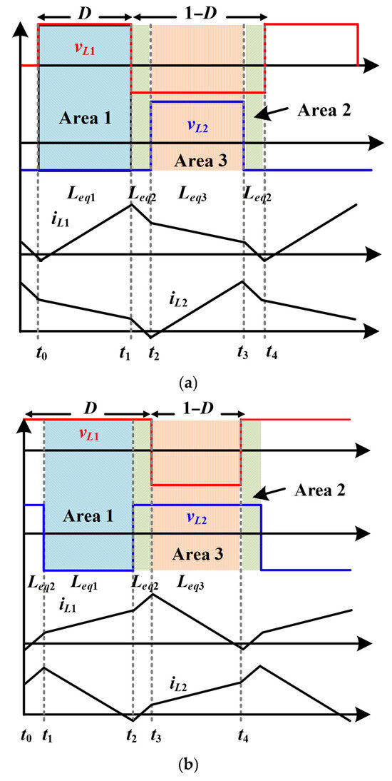
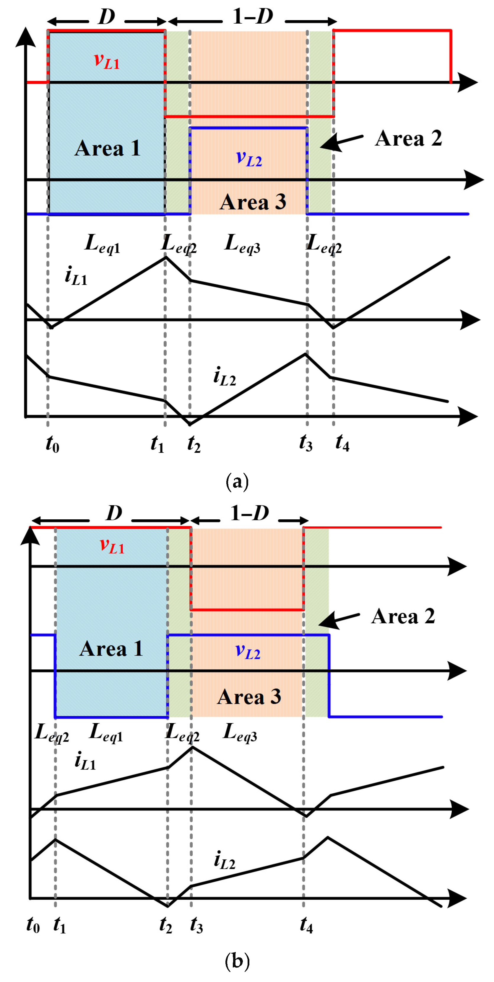
The voltage and current waveforms of the three different conditions during a switching cycle are shown in Figure 2. It can be seen that, during a switching cycle, the inductor current operates in multiple stages.
Figure 2.
Voltage and current waveforms of steady state. (a) D < 0.5. (b) D > 0.5.
The first type of equivalent inductance Leq1 is shown in area 1, when vL1 is equal to Vi −Vo and vL2 is equal to −Vo. The second type of equivalent inductance Leq2 is shown in area 2, when vL1 is equal to vL2. The third type of equivalent inductance Leq3 is shown in area 3, when vL1 is equal to −Vo and vL2 is equal to Vi − Vo. The three equivalent inductances are listed in Table 1, respectively.
Table 1.
Equivalent Inductance.
2.2. Dynamic Analysis
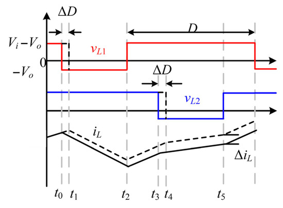
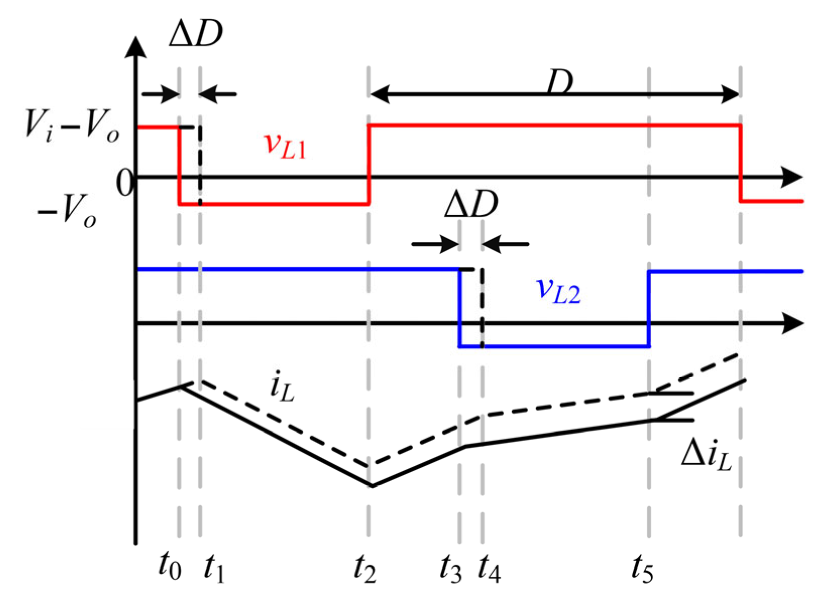
The dynamic process waveforms are shown in Figure 3. The black dashed line represents the inductor current of the dynamic process. The duty cycle difference is defined as ΔD. During one switching cycle, the current difference ΔiL can be divided into five parts, which can be expressed as
Figure 3.
Dynamic process waveforms.
By summing Equation (6), the inductor current difference after one switching cycle can be calculated as
The steady-state inductor current satisfies the volt second balance principle, hence the current difference within one switching cycle is equal to zero, which can be expressed as
Finally, combining (7) and (8), the dynamic process inductor current state equation can be derived as
where Leq2 is the equivalent inductance when vL1 is equal to vL2.
According to (9), it can be seen that the response speed of inductor current is inversely proportional to Leq2. When the coupling coefficient is less than zero, the equivalent inductance Leq2 will decrease relative to self-inductance L. Therefore, the interleaved Buck converter with negatively coupled inductor has a higher current response speed.
2.3. ZVS Analysis
For the coupled inductor-based interleaved Buck converter, the calculation of ZVS conditions will be more complex because the inductor current operates in multiple different modes. In this paper, the conditions of ZVS will be unified and easily implemented in digital processors.
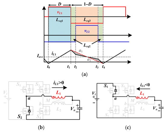
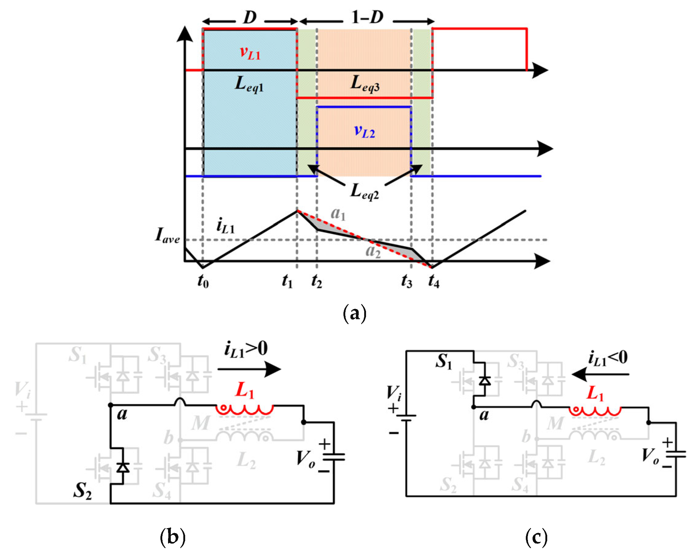
The equivalent circuit modes and operating waveforms of ZVS are shown in Figure 4. For S2, during the dead time at t1, iL1 must be greater than zero, which will flow through the body diode of S2, as shown in Figure 4b. Therefore, S2 must achieve ZVS at any voltage and power. For S1, in order to achieve ZVS, the inductor current needs to be reversed within one switching cycle, as shown in Figure 4c. Therefore, the peak-to-peak value of the inductor current Ipp needs to be higher than twice the average value Iave. Hence, it is more difficult to achieve ZVS under full load.
Figure 4.
ZVS operation. (a) ZVS waveforms. (b) ZVS operation equivalent circuit of S2. (c) ZVS operation equivalent circuit of S1.
Under BCM, Ipp is approximately equal to 2 × Iave. This condition can achieve ZVS and reduce circulating current. Therefore, it is necessary to calculate the appropriate switching frequency based on Iave.
During a switching cycle, the inductor current operates in multiple stages. Due to the symmetry of the two bridges, in Figure 4a, the shaded areas a1 and a2 are equal. Therefore, the operating modes of the inductor current in multiple stages can be equivalent to the red dashed line. Taking iL1 as an example (D < 0.5), the peak-to-peak value of inductor current can be calculated as
According to the ZVS condition, the switching frequency range can be derived as
where Iave is equal to Io/2.
Similarly, when D > 0.5, the range of switching frequency can be expressed as
When the switching frequency is too low, although ZVS can be achieved, higher circulating currents will be generated. Therefore, the switching frequency is typically set near its upper limit. Combining (11) and (12), the calculation of switching frequency requires consideration of the correct equivalent inductance value at different duty cycles, which can be expressed as
2.4. Digital BCM Control Strategy
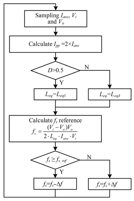
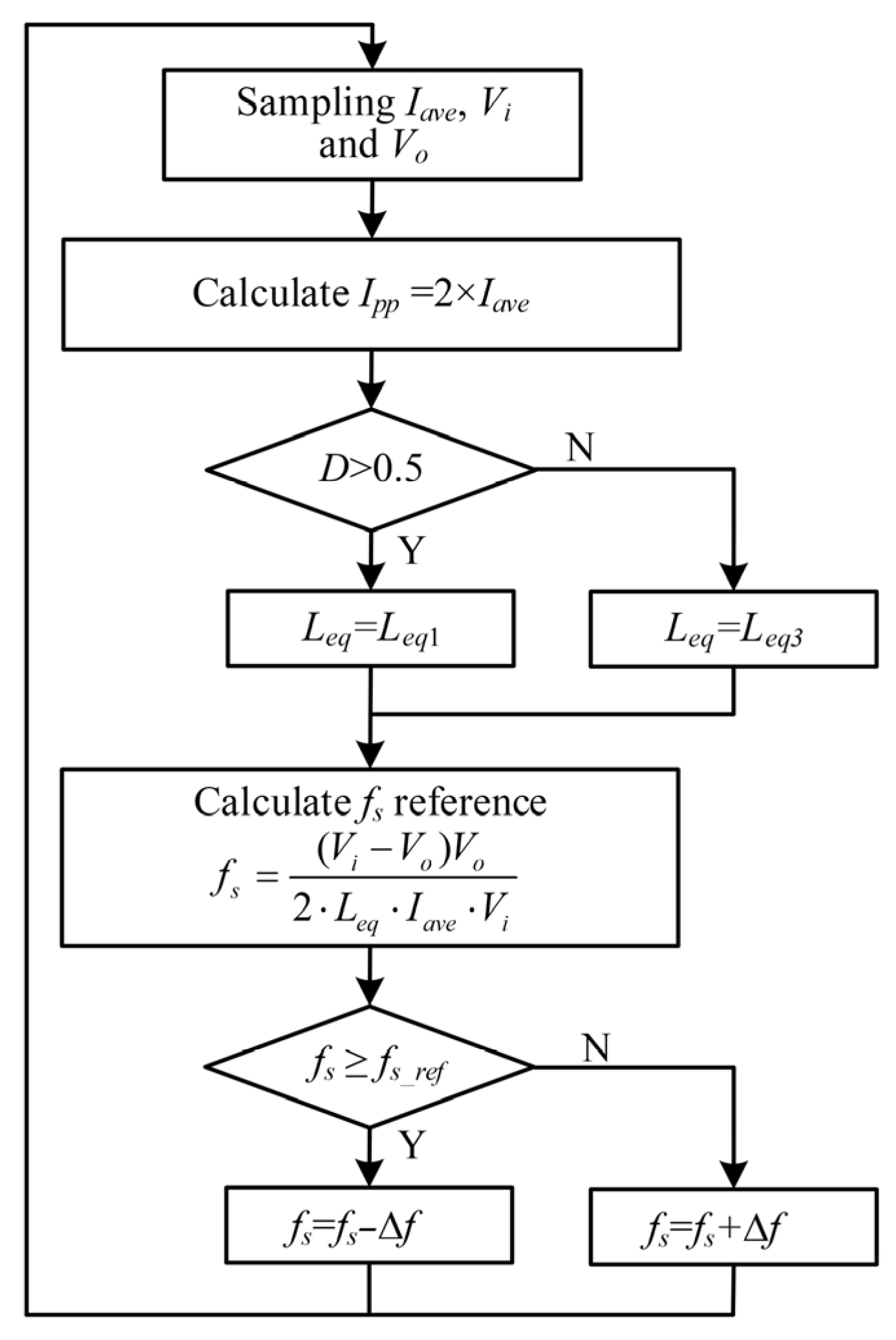
In this paper, the traditional average current control can be adopted, hence, Iave, Vin and Vo need to be sampled by the digital processor. In addition, Iave can be obtained by sampling inductor current at the duty cycle midpoint. The detailed steps are shown in Figure 5. The proposed variable frequency control mainly consists of the following five steps:
Figure 5.
The flow chart of variable frequency control.
Step 1: Sample the average value of inductor current Iave, input voltage Vi and output voltage Vo.
Step 2: Calculate Ipp.
Step 3: Determine Leq value.
Step 4: Calculate the switching frequency reference by (13).
Step 5: Adjust the switch frequency.
3. Coupled Inductor Design
3.1. Optimal Coupling Coefficient Design
According to (13), under BCM control, as the operating voltage (duty cycle) varies widely, the switching frequency will also be adjusted widely. It will bring challenges to the design of magnetic components and driving circuits. Among them, the equivalent inductance value Leq will also change with the duty cycle, hence the range of switching frequency can be minimized by designing the optimal coupling coefficient.
Substitute the expression of Leq into (13), which can be rewritten as
where Po is the entire output power of the two phases.
Equation (14) shows that the switching frequency is inversely proportional to the out-put power. At full load, the switching frequency is the lowest, which is also the most difficult to achieve ZVS. Therefore, it is necessary to design parameters under full load.
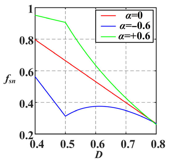
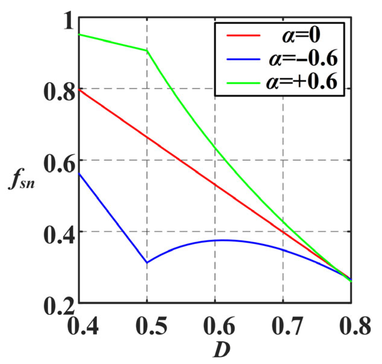
Under full load, when the output voltage Vo and self-inductance L are fixed, the switching frequency needs to be adjusted with the duty cycle D. The purpose of designing the optimal coupling coefficient is to minimize the switching frequency range variation with duty cycle. By setting to 1, the normalized switching frequency fsn can be obtained as
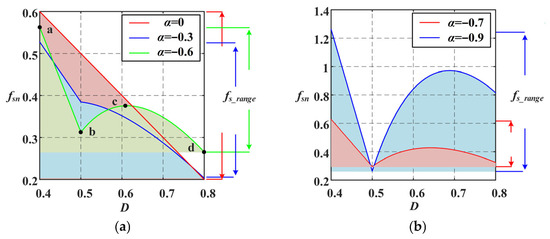
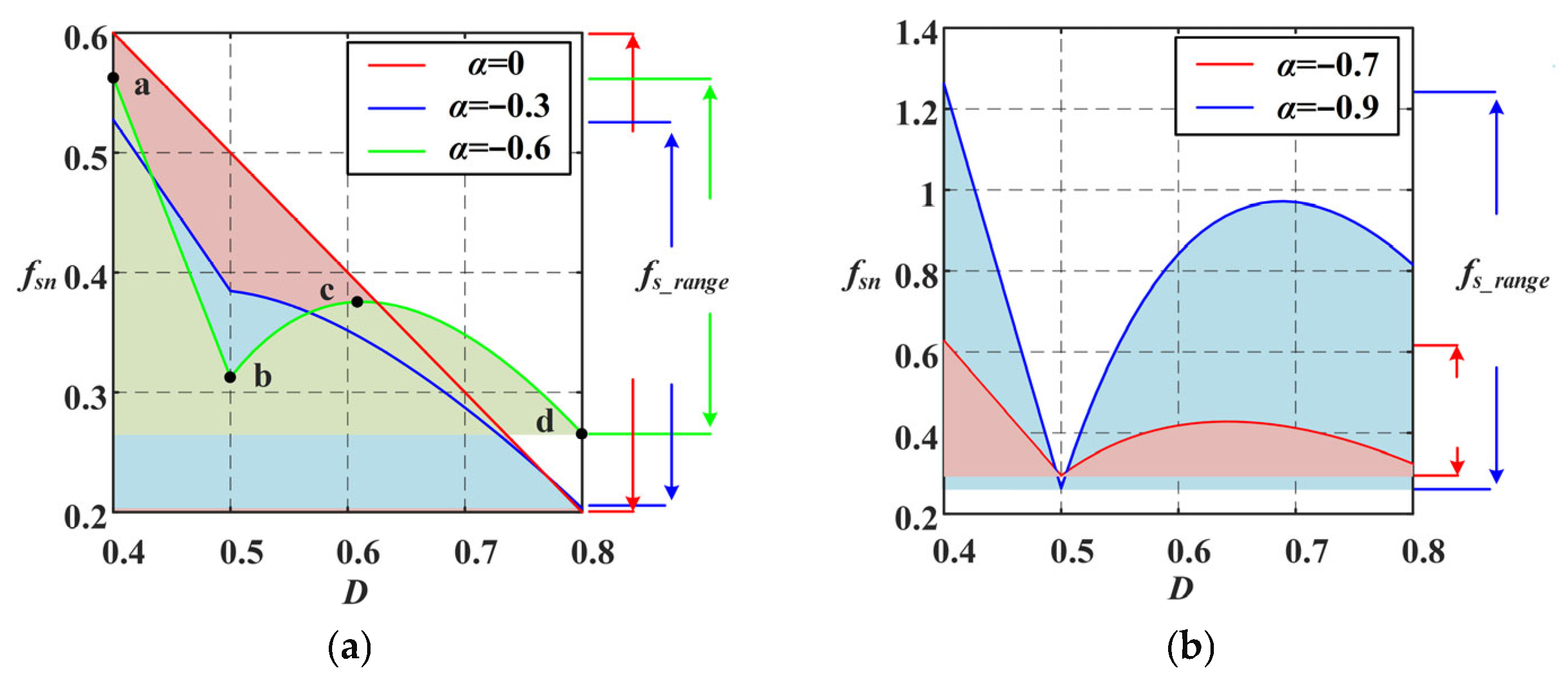
Base on (15), the relationship between D and the normalized switching frequency fsn under different coupling coefficients α is shown in Figure 6.
Figure 6.
Normalized switching frequency under different coupling coefficients and duty cycles. (a) α = 0, α = −0.3 and α = −0.6. (b) α = −0.7 and α = −0.9.
When D < 0.5, the D − fs curve is a monotonically decreasing function. Therefore, the switching frequency of point a (Dmin) must be greater than that of point b (D = 0.5).
When D > 0.5, the D − fs curve has a maximum at point c (f’sn = 0). And it also has another boundary value at point d (Dmax).
To sum up, the highest frequency may occur at point a (Dmin) or point c (f’sn = 0), and the lowest frequency may occur at point b (D = 0.5) or point d (Dmax). Taking the experimental prototype built in this paper as an example, the duty cycle range is approximately 0.4~0.8.
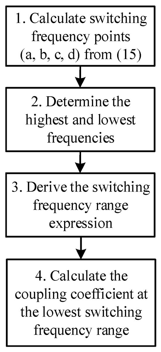
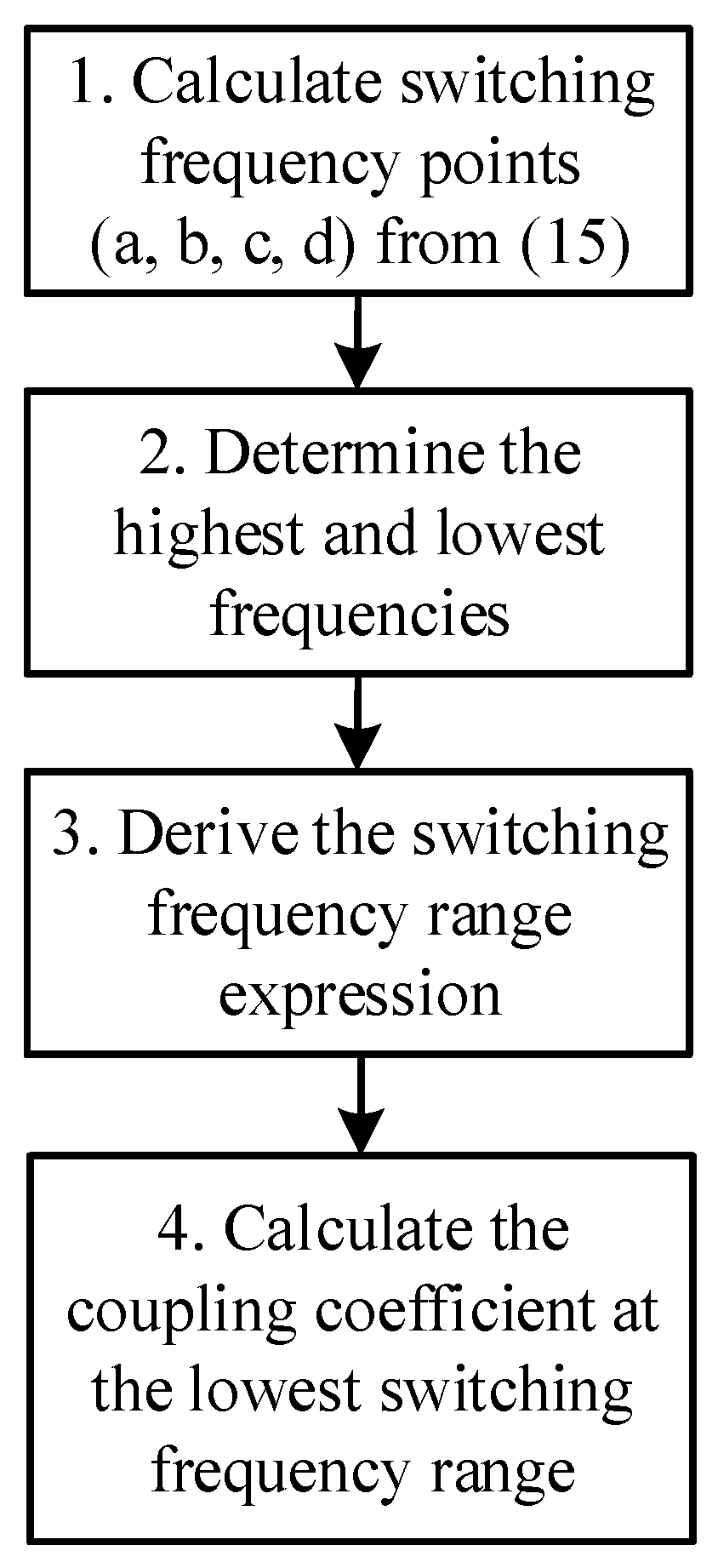
The flowchart for designing the optimal coupling coefficient is shown in Figure 7. Firstly, based on the piecewise function (15), the switching frequency points (a, b, c, d) need to be solved. Secondly, calculate the values of four points (a, b, c, d) and determine the highest and lowest frequencies. Thirdly, the frequency range expression can be obtained by subtracting the lowest frequency from the highest frequency. Finally, calculate the coupling coefficient at the lowest frequency range.
Figure 7.
Design flowchart.
The duty cycle range in this paper is 0.4–0.8. Taking this as an example, the optimal coupling coefficient can be calculated through the following four steps.
- (1)
- Calculate frequency value: The switching frequency of the four points can be calculated as
- (2)
- Determine the maximum and minimum values of switch frequency: fsna is always greater than fsnc; therefore, the maximum switching frequency is equal to fsna. In addition, when α ≤ −2/3, fsnb < fsnd, and when α > −2/3, fsnb > fsnd. Therefore, the maximum and minimum values of the switching frequency can be expressed as:
- (3)
- Derive frequency range expression: After subtracting the minimum value from the maximum value, the range of switching frequency can be derived as
- (4)
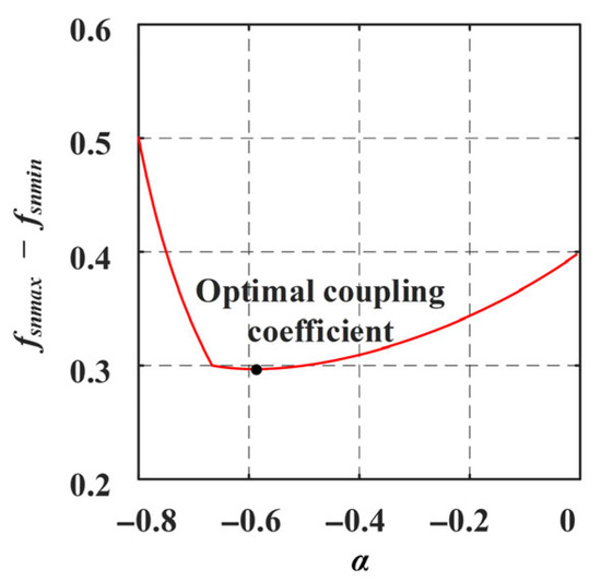
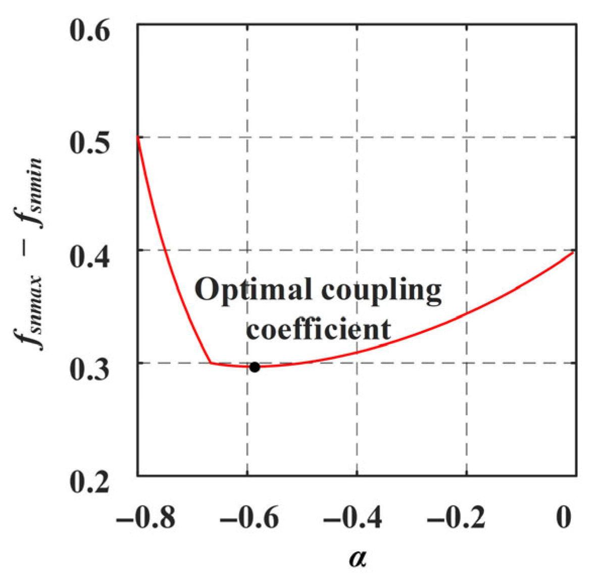
- Calculate the optimal coupling coefficient: According to (16), the relationship between coupling coefficient and switching frequency range is shown in Figure 8. It can be seen that when the coupling coefficient α is approximately −0.6, the range of switching frequencies is minimal. Especially compared with separate inductor designs (α = 0), the adjustment range of switching frequency is significantly reduced. In addition, when the coupling coefficient is around 0.6, the slope of the frequency range function is nearly flat. Even considering a 10% design error, the range of switching frequency variation is very low.Figure 8. The relationship between coupling coefficient and switching frequency range.
3.2. Self-Inductance Design
According to (13), after determining the coupling coefficient, at full load and lowest switching frequency, the self-inductance range can be expressed as
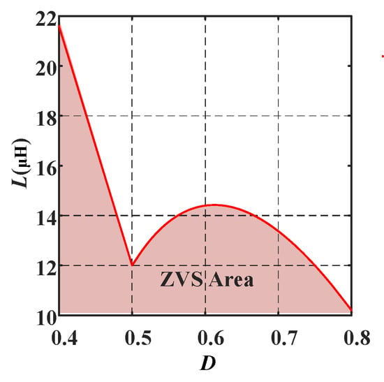
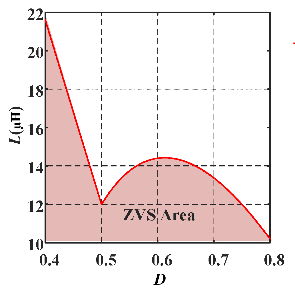
Based on (19), the self-inductance range is shown in Figure 9. Below the red curve is the ZVS area. In addition, a too low inductance value can lead to a higher circulating current, hence the self-inductance value needs to be designed near the upper boundary value. In this paper, the self-inductance value is designed to be about 10 μH.
Figure 9.
Range of self-inductance values.
3.3. Coupled Inductor Structure Design
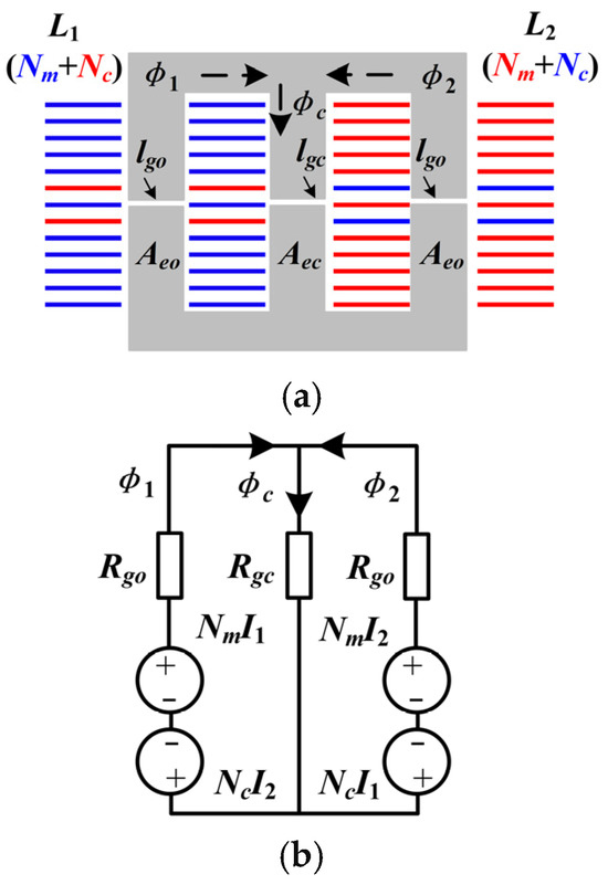
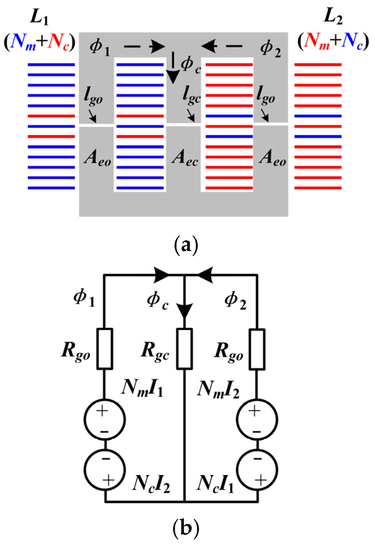
In order to increase the coupling degree between the primary and secondary sides, a coupled inductor with interleaved winding structure is adopted in this paper, as shown in Figure 10a. The two windings are wound on the outer side leg of the magnetic core. The total turns are (Nm + Nc). Taking winding L1 as an example, on the left leg, the number of turns in the main winding is Nm. On the right leg, the number of turns crossing with winding L2 is Nc. Due to the symmetry of the coupled inductor structure, winding L2 has a similar distribution. The air gap length of both outer legs is lgo, and the air gap length of the central leg is lgo. In addition, the cross-sectional areas of the outer leg and the central leg are Aeo and Aec, respectively.
Figure 10.
Coupled inductor structure. (a) Coupled inductor with interleaved winding structure. (b) Equivalent magnetic circuit.
According to the structure of the winding, the equivalent magnetic circuit is shown in Figure 10b. The magnetic flux of the outer leg is ϕ1 and ϕ2, respectively. The magnetic flux of the central leg is ϕc. The magnetic resistance of the outer leg and the central leg are Rgo and Rgc, respectively. According to the superposition theorem, ϕ1, ϕ2 and ϕc can be calculated as
According to the definition, self-inductance and mutual inductance can be expressed as
After the self-inductance, mutual-inductance, and number of turns are determined, the magnetic reluctance Rgo and Rgc can be solved. Then, based on the relationship between air gap and magnetic resistance, the air gap length can be calculated as
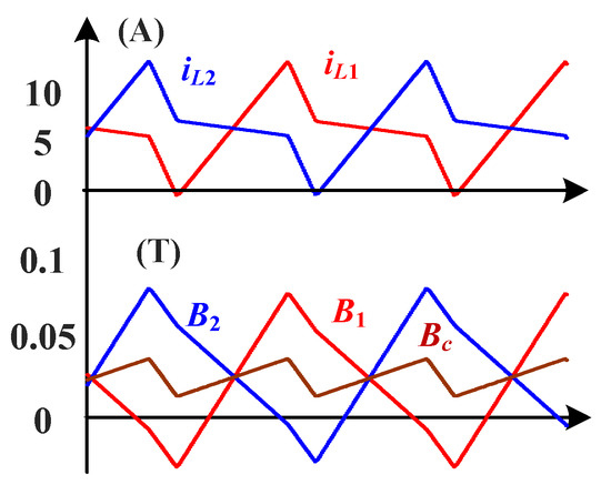
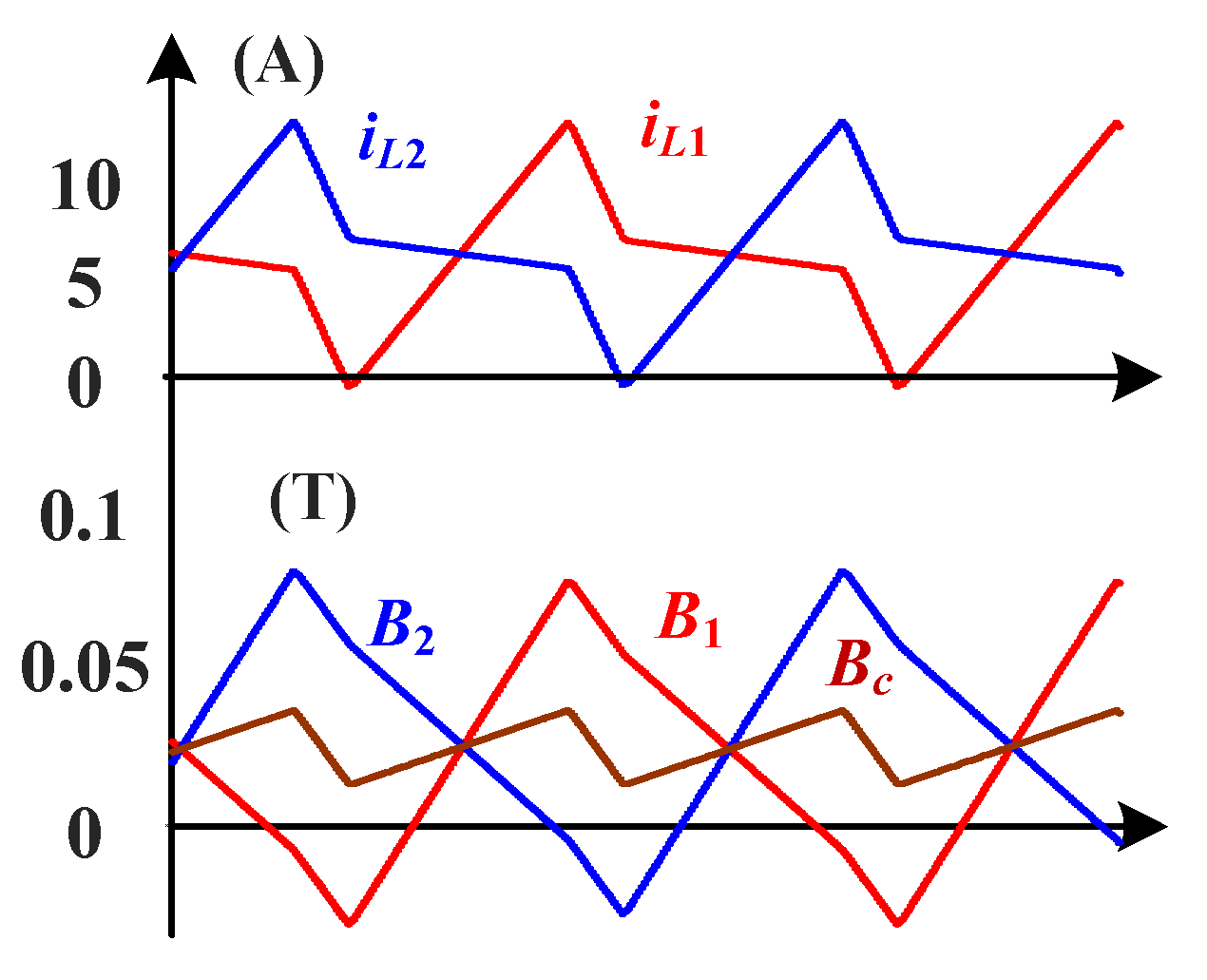
In this paper, the magnetic core type EE4220 is adopted. The main winding turns number Nm is 11, and the crossing winding turns number Nc is 2. The outer leg and the center leg air gap length are both approximately 1.5 mm. According to the design parameters, the waveforms of magnetic flux density and current are shown in Figure 11. The magnetic flux density peak to peak value can be deduced as (Bmax − Bmin)/2. In addition, in the proposed coupled inductor structure, the magnetic flux density of the center leg is reduced due to the 180 degree phase difference of the inductor current. But the magnetic flux density of the outer leg is higher.
Figure 11.
Magnetic flux density waveforms.
3.4. ZVS Range
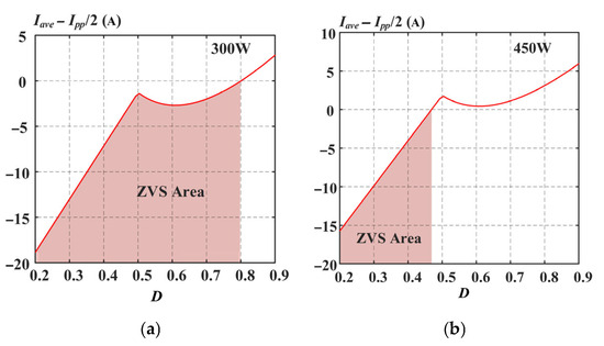
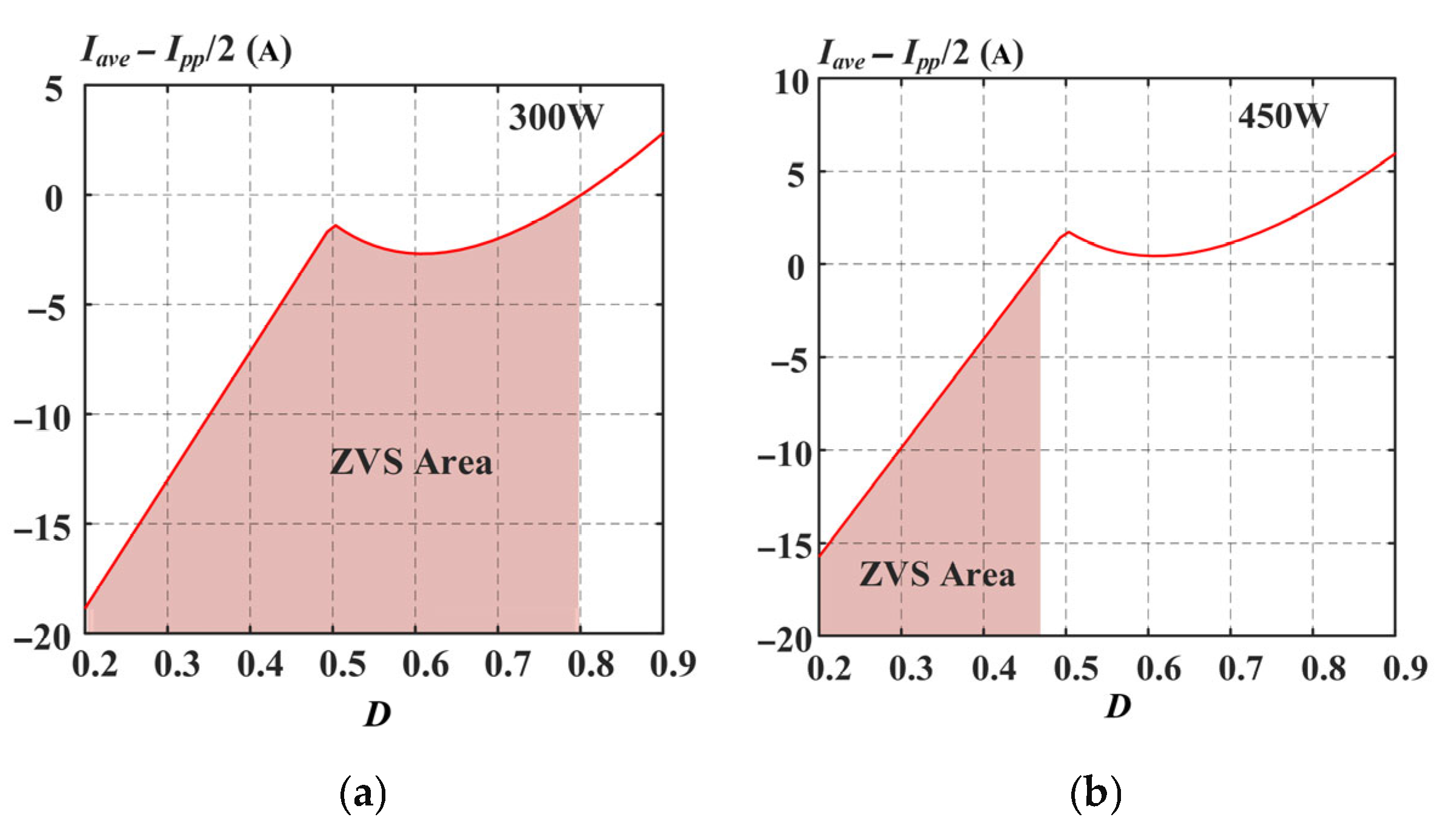
In this paper, the lowest frequency is 50 kHz, with a duty cycle range of approximately 0.4–0.8 (input voltage 30–60 V, output voltage 24 V). The ZVS range figures at the rated power (300 W) and 1.5 times overload (450 W) are shown in Figure 12. According to ZVS analysis, Iave − Ipp/2 needs to be less than zero to achieve ZVS. Under the rated power (300 W), ZVS can be implemented when the duty cycle is less than 0.8. When the duty cycle is greater than 0.8, ZVS will be lost. In addition, at higher power,, such as 1.5 times overload (450 W), ZVS can only be implemented when the duty cycle is less than 0.45. Hence, ZVS is more difficult to achieve at high power.
Figure 12.
ZVS range. (a) 300 W. (b) 450 W.
3.5. Characteristic Comparison
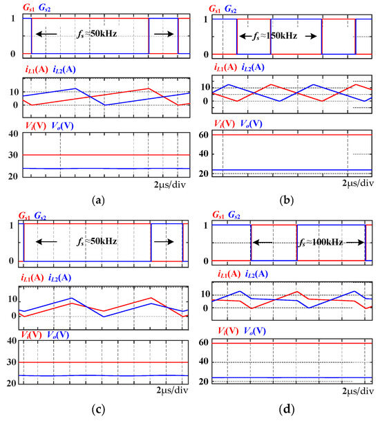
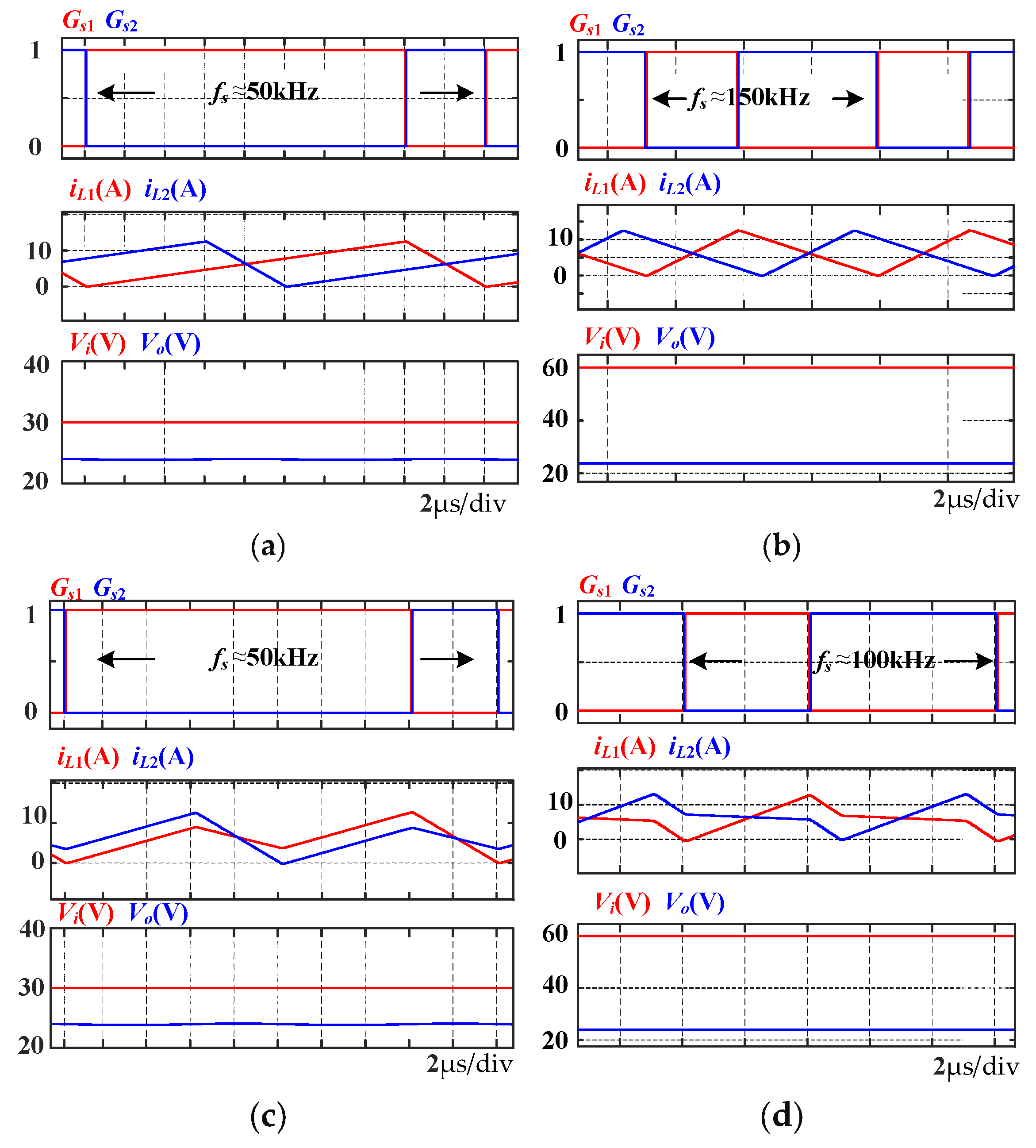
Under the same parameters of voltage range, operating power, and minimum switching frequency, a comparison is conducted among the following three types of Buck converters with different inductors: separate inductors, positively coupled inductors (α = 0.6), and negatively coupled inductors (α = −0.6).
The simulation waveforms of the negatively coupled inductor and the separate inductor are shown in Figure 13. In addition, the detailed comparative data are shown in Table 2. Regarding current ripple, under the control of the BCM, in order to achieve ZVS, the peak-to-peak value of the inductor current in each phase is approximately equal to twice the average value. Therefore, the three types of current ripple and circulating current are completely identical. However, in order to achieve BCM control, the switching frequency ranges are different. The negatively coupled inductor with the optimal coupling coefficient has the narrowest frequency range, as shown in Figure 14. Furthermore, for dynamic equivalent inductance (L(1 + α), as shown in Table 1), using positively coupled inductor will increase the equivalent inductance. Therefore, dynamic response is decreased.
Figure 13.
Simulation waveforms (300 W). (a) Separate inductor, 30 V. (b) Separate inductor, 60 V. (c) Coupled inductor, 30 V. (d) Coupled inductor, 60 V.
Table 2.
Characteristic comparison.
Figure 14.
Switching frequency range.
3.6. Loss Analysis and Comparison
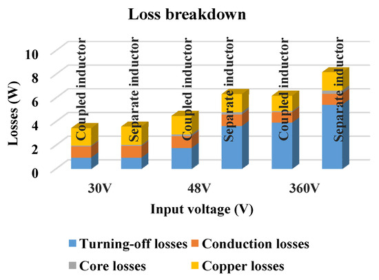
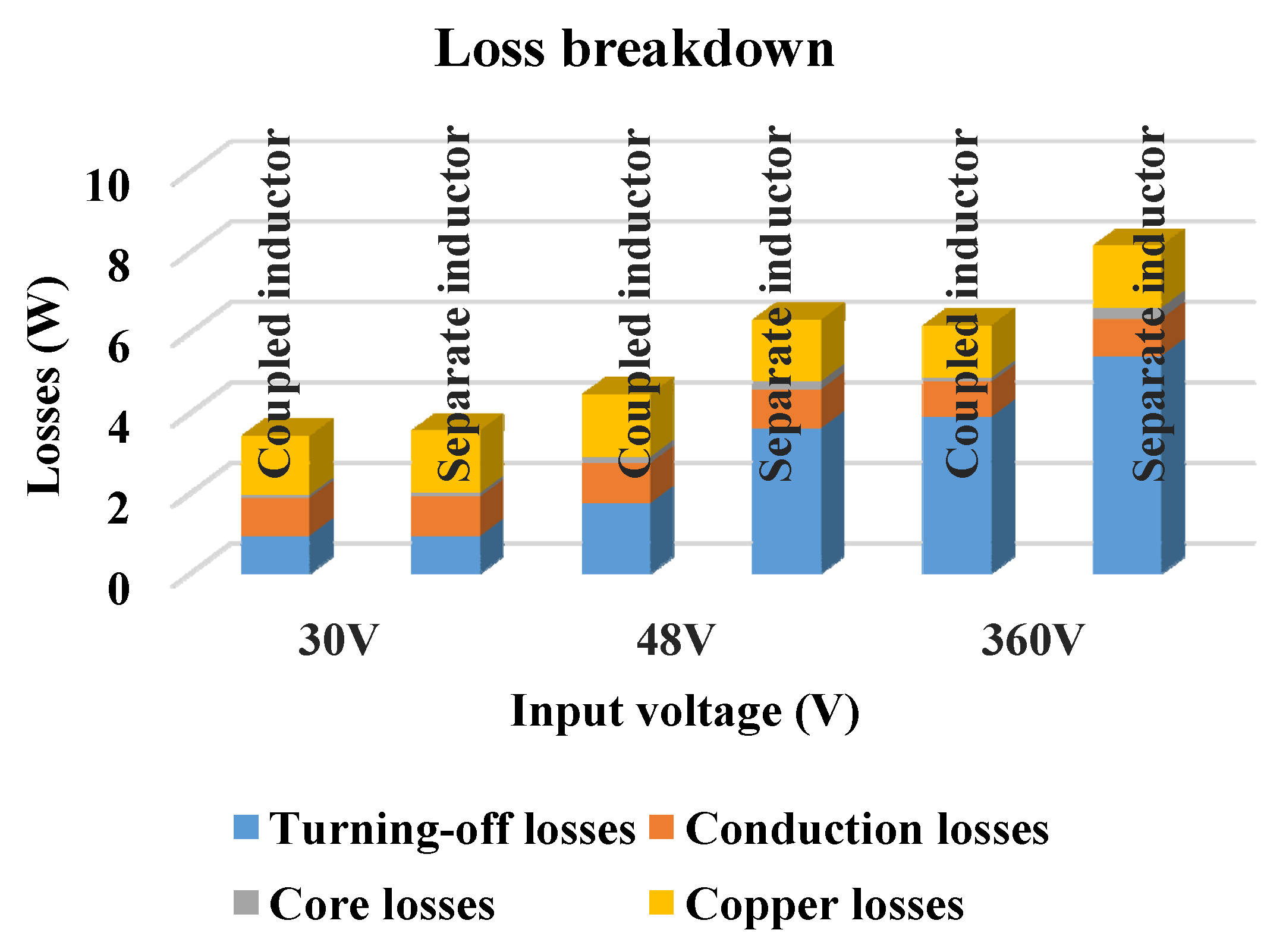
The theoretical loss analysis results are shown in Figure 15. All MOSFETs can achieve ZVS; therefore, the turning-on loss of MOSFETs can be ignored. The main losses include turning-off loss, conduction loss, core loss and copper loss. The loss analysis results are compared with the separate-inductor converter. Among them, the separate inductors are designed with two EE30 magnetic cores. The overall cost is similar to that of one EE4220 magnetic core. Due to the adoption of the optimal coupling coefficient design, the switching frequency range is narrower, and the proposed converter can achieve BCM at lower frequency. Therefore, the turning off losses and core losses are lower than in the case with the separate-inductor converter, and the overall efficiency of the proposed converter is also higher.
Figure 15.
Loss analysis.
In addition, the main losses of the converter are conduction loss and turn-off loss. This is because under BCM control, the peak-to-peak value of the inductor current is relatively high (twice the average value). Therefore, the proposed solution is more suitable for low-current applications.
4. Experimental Verification
In order to validate the performance of optimal design with the coupling coefficient, an experimental prototype is built. The detailed parameters are listed in Table 3.
Table 3.
Parameters of the Experimental Prototype.
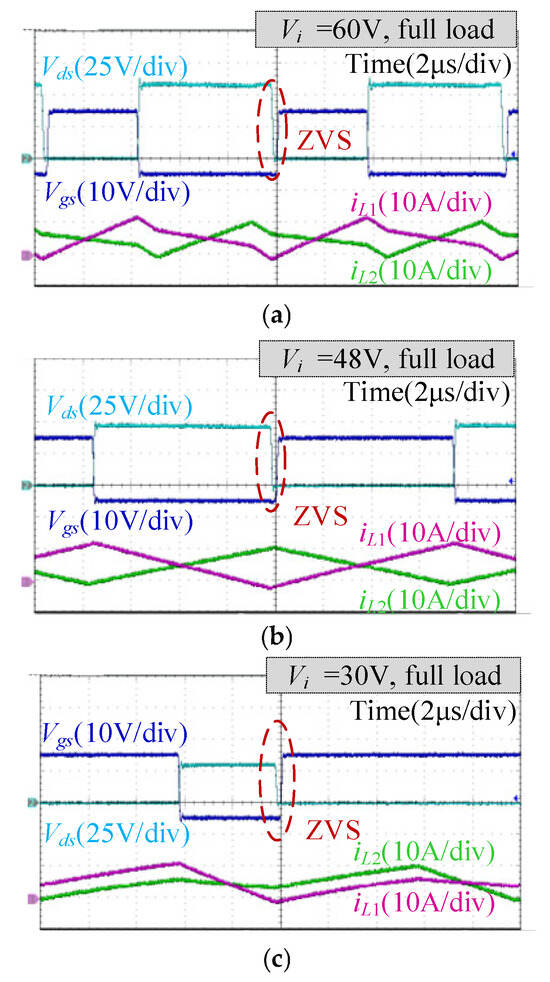
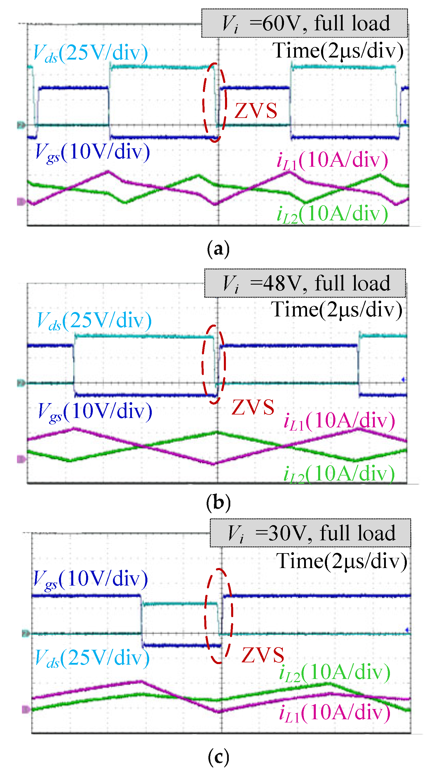
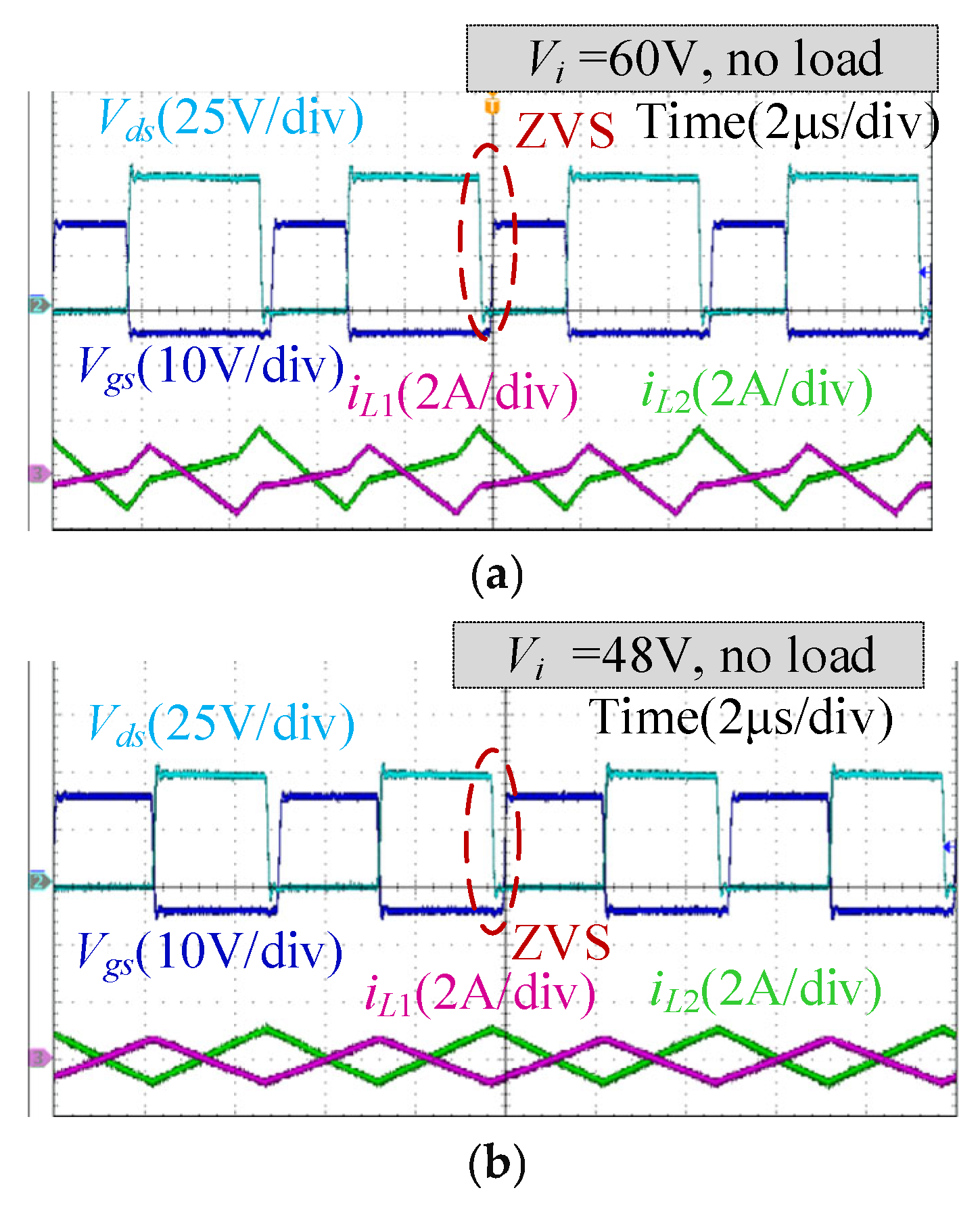
The full load steady-state operating waveforms with different loads and input voltages are shown in Figure 16. It can be seen that the phase difference between the two-phase inductor currents is 180 degrees. And the inductor current has multiple stages within one switching cycle, which is consistent with theoretical analysis. Under BCM control, the inductor current valley value is slightly below zero. The drain-source voltage of MOSFET has already dropped to zero before turning on, hence ZVS can be achieved. In addition, the switching frequency will be adjusted at different voltages to achieve BCM operation. Therefore, the valley value of inductor current is relatively fixed. Under the optimal coupling coefficient design, the lowest switching frequency is approximately 50 kHz (Vi = 30 V) and the highest switching frequency is approximately 100 kHz (Vi = 60 V). The experimental results are consistent with the simulation results in Figure 13. Under the proposed optimization design, the switching frequency range is relatively narrow when operating at full load.
Figure 16.
Full-load steady-state waveforms. (a) Input 60 V. (b) Input 48 V. (c) Input 30 V.
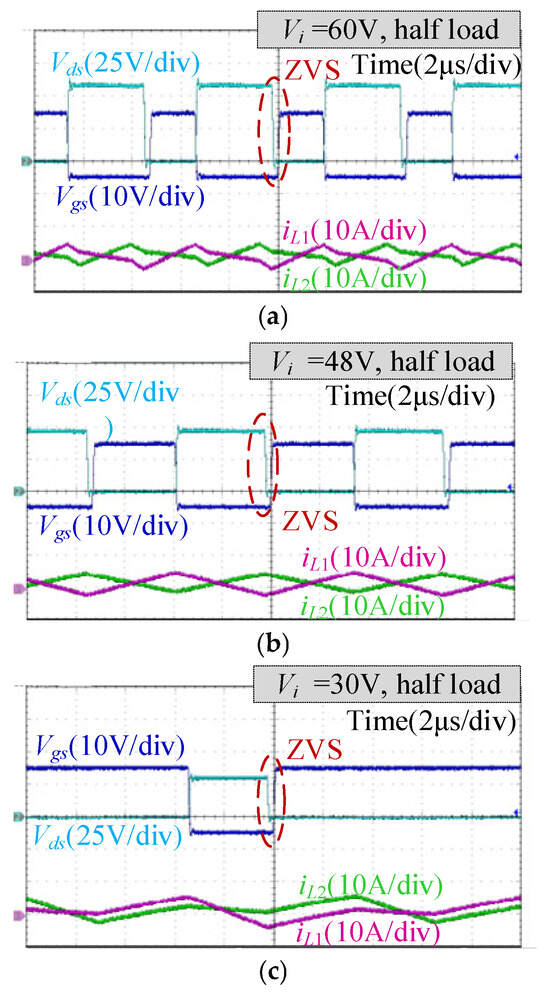
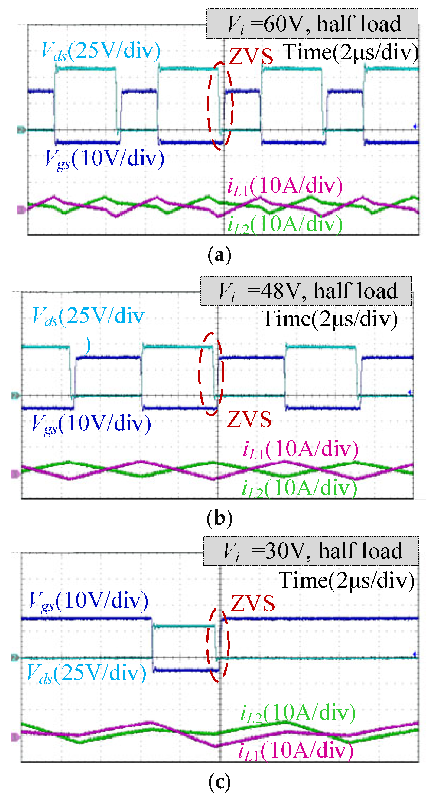
The experimental waveforms of half-load operation are shown in Figure 17. Because the average value of inductor current decreases, the switching frequency needs to be increased. In this way, while maintaining ZVS operation, the ripple of inductor current is reduced to decrease conduction loss.
Figure 17.
Half-load steady-state waveforms. (a) Input 60 V. (b) Input 48 V. (c) Input 30 V.
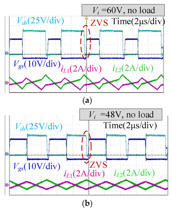
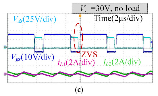
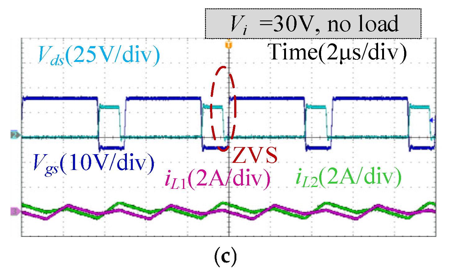
The waveform of the no-load experiment is shown in Figure 18. It can be seen that under no-load conditions, ZVS is very easy to be achieved because the average value of inductor current is close to zero. In order to reduce the circulating current, the switching frequency will be adjusted to the highest level (200 kHz).
Figure 18.
No-load steady-state waveforms. (a) Input 60 V. (b) Input 48 V. (c) Input 30 V.
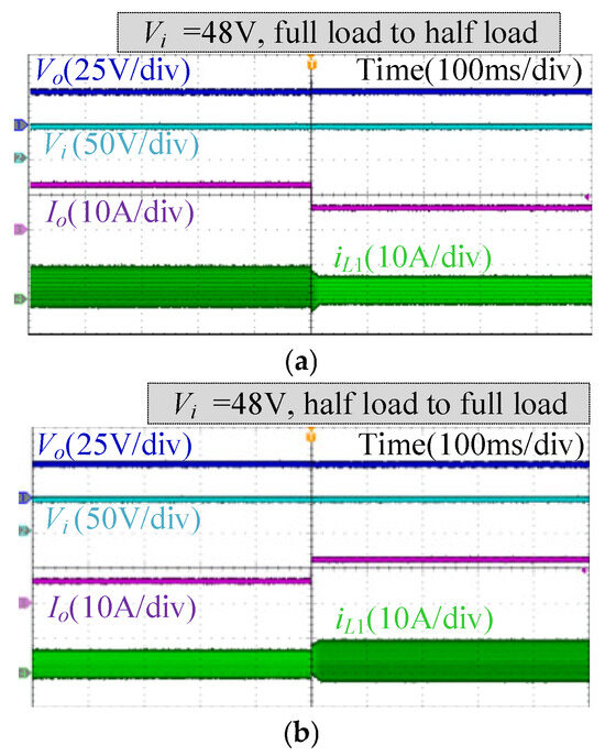
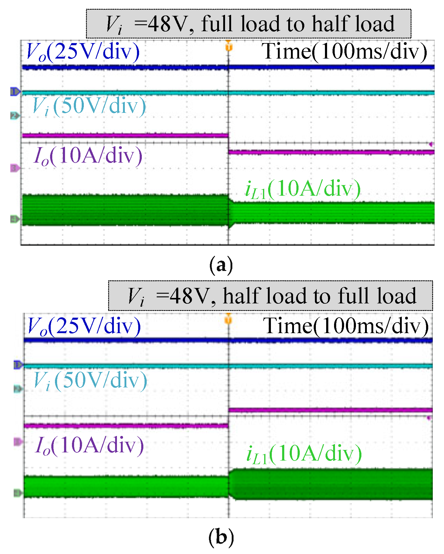
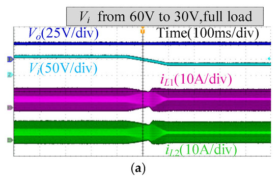
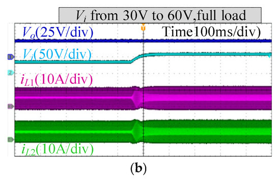
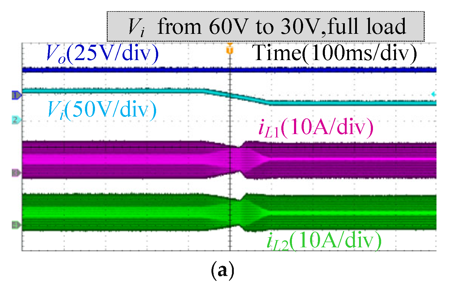
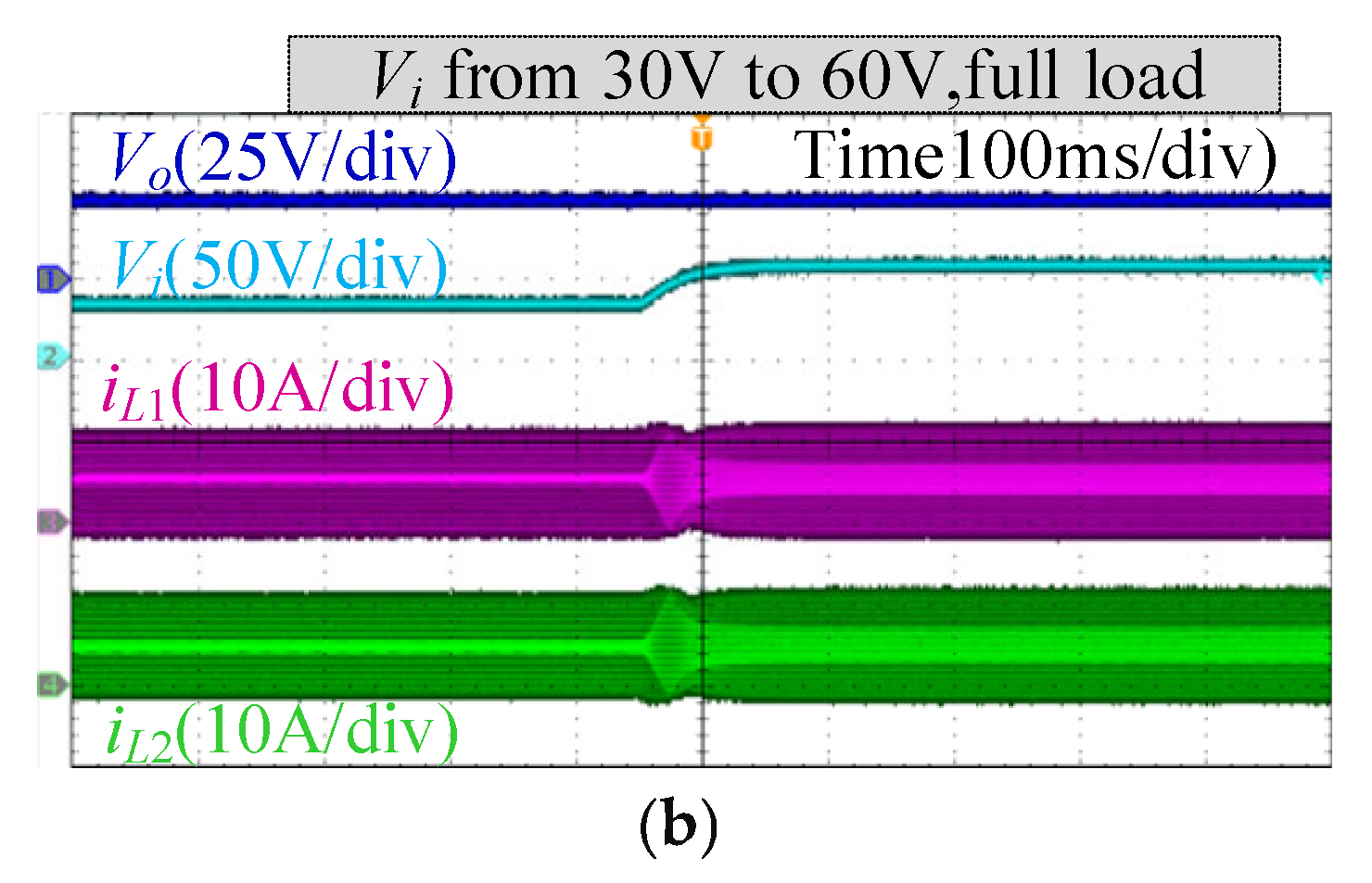
The dynamic waveforms are shown in Figure 19 and Figure 20. Under digital BCM control, adjusting the switching frequency will cause the inductor current to enter a transient state. In order to prevent frequency adjustment from disturbing the voltage and current control loops, the switching frequency is adjusted using a ramp function. In this paper, the control and sampling periods are both 20 kHz. In addition, the adjustment step of the switching frequency is 0.1 kHz. When the load switches from full load to half load, the switching frequency is increased to reduce the circulating current. Similarly, when the load is increased, the switching frequency will be reduced to achieve ZVS. The adjustment time for current ripple and switching frequency is approximately 20 ms. When the input voltage changes, the switching frequency also needs to be adjusted, and the ripple of the inductor current remains constant.
Figure 19.
Load-switching waveforms. (a) Full load to half load. (b) Half load to full load.
Figure 20.
Input voltage switching waveforms. (a) 60 V to 30 V. (b) 30 V to 60 V.
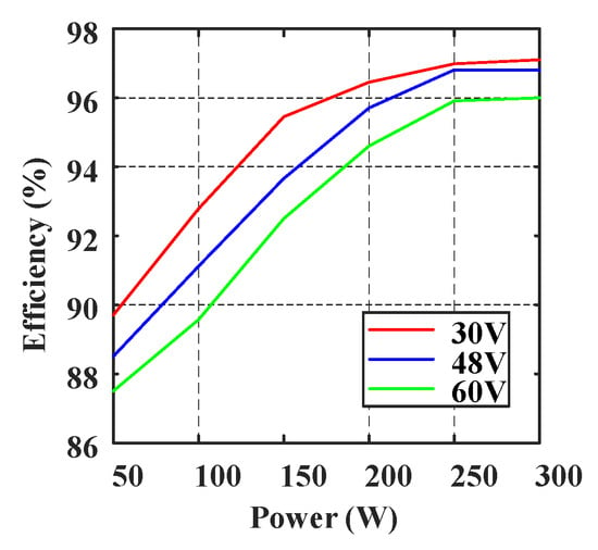
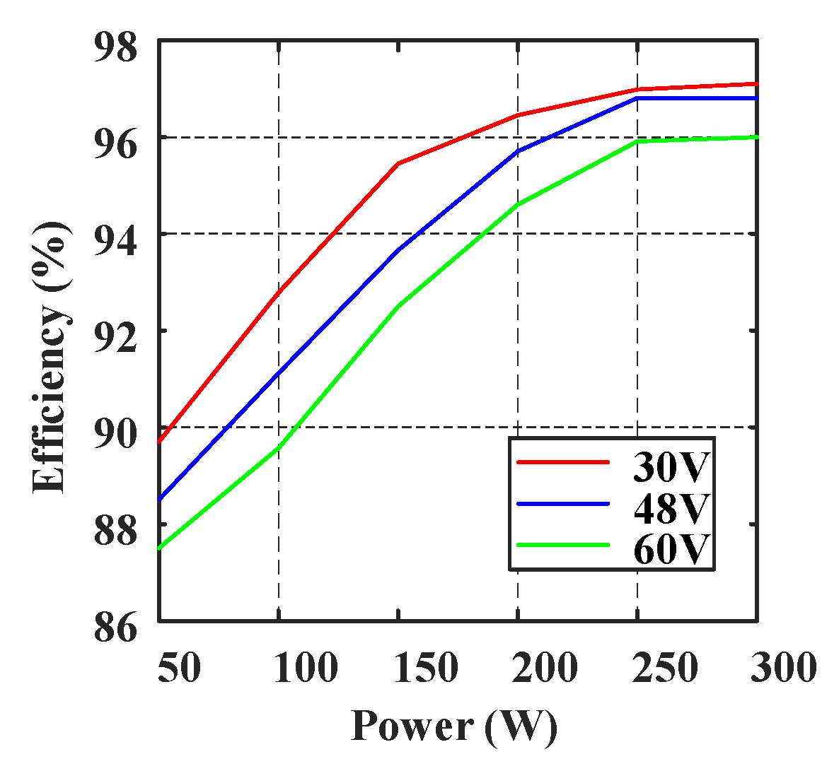
The measurement efficiency curves are shown in Figure 21. At low input voltages, the switching frequency is correspondingly reduced, resulting in lower turn-off losses and core losses. Conversely, under high input voltages, an increased switching frequency is required to reduce current ripple, which leads to relatively higher turn-off and core losses. Overall, the operating efficiency of the converter is higher at low input voltages.
Figure 21.
Measurement efficiency.
5. Conclusions
In this paper, an interleaved Buck converter with negatively coupled inductor and optimal coupling coefficient is proposed. The proposed converter operates under BCM to achieve ZVS. A fully digital adaptive frequency control strategy is implemented, eliminating the need for ZCD circuits or auxiliary components. Compared with the analog scheme, the proposed method only requires sampling the average values of voltage and current, which can reduce the sensitivity to sampling noise. In addition, in order to reduce the adjustment range of the switching frequency, a design method for the optimal coupling coefficient is proposed. Compared with separate-inductor designs, the adjustment range of switching frequency is significantly reduced. A 300 W experimental prototype was built, and the experimental results validated the effectiveness of the proposed solution.
Author Contributions
Conceptualization, J.X., X.C. and X.H.; methodology, J.X. and X.C.; writing—original draft preparation, J.X. and X.C.; writing—review and editing, J.X. and X.H. All authors have read and agreed to the published version of the manuscript.
Funding
This work was supported in part by the National Natural Science Foundation of China under Grant 52407232, 52307232, Key Research and Development Program of Hunan Province under Grant 2024JK2013, the Hunan Provincial Natural Science Foundation of China under Grant 2026JJ60192, 2024JJ4055, and the State Key Laboratory of Power System Operation and Control under Grant SKLD23KM12.
Data Availability Statement
The original contributions presented in the study are included in the paper. Further inquiries can be directed to the corresponding author.
Conflicts of Interest
The authors declare no conflicts of interest.
Nomenclature
| Vi, Vo | Input voltage and output voltage |
| Po | Output power |
| L1, L2 | Self-inductance |
| M | Mutual inductance |
| α | Coupling coefficient |
| vL1, vL2 | Terminal voltage of coupled inductor windings L1 and L2 |
| iL1, iL2 | Current of coupled inductor windings L1 and L2 |
| D | Duty cycle of S1 and S3 |
| Ipp | Peak to peak value of inductor current |
| Iave | Average value of inductor current |
| fsn | Normalized switching frequency |
| Nm | Main winding turns number |
| Nc | Crossing turns number |
| lgo, lgc | Air gap length of outer legs and central leg |
| Aeo, Aec | Cross-sectional areas of outer leg and central leg |
| ϕ1, ϕ2, ϕc | Magnetic flux of the outer leg and central leg |
References
- Jia, X.; Sha, D.; Zhao, Y. Unified One-Cycle Control for Fully Digitalized ZVS Four-Switch Buck–Boost Converter During Bidirectional Power Flow Transition. IEEE Trans. Power Electron. 2024, 39, 11295–11307. [Google Scholar] [CrossRef] [Scilit]
- Abdurraqeeb, A.M.; Al-Shamma’a, A.A.; Alkuhayli, A.; Noman, A.M.; Addoweesh, K.E. RST Digital Robust Control for DC/DC Buck Converter Feeding Constant Power Load. Mathematics 2022, 10, 1782. [Google Scholar] [CrossRef] [Scilit]
- Zhao, Z.; Luo, P.; Zhang, Z.; Fan, J.; Zhang, B.; Chen, X. A Peak-Valley Current-Mode Buck Converter With 3% to 95% Duty Cycle. IEEE Trans. Circuits Syst. II Express Briefs 2025, 72, 328–332. [Google Scholar] [CrossRef] [Scilit]
- Zambrano-Gutierrez, D.F.; Cruz-Duarte, J.M.; Castañeda, H.; Avina-Cervantes, J.G. Optimization of Adaptive Sliding Mode Controllers Using Customized Metaheuristics in DC-DC Buck-Boost Converters. Mathematics 2024, 12, 3709. [Google Scholar] [CrossRef] [Scilit]
- Zhang, J.; Li, Y.; Wan, J.; Zhao, B.; Zhang, Y.; Liu, F. A New Active Clamp Zero-Voltage-Transition Cell for Non-Isolated DC-DC Converter with Low Current Stress. CPSS Trans. Power Electron. Appl. 2025, 10, 231–240. [Google Scholar] [CrossRef] [Scilit]
- Mohammadi, M.R. An active-clamping ZVS interleaved buck/boost bi-directional converter with one auxiliary switch. IEEE Trans. Ind. Electron. 2020, 67, 7430–7438. [Google Scholar] [CrossRef] [Scilit]
- Pal, A.; Saha, S.S. Novel Zero-Voltage Zero-Current Transition Buck Converter With Minimal Impact of Active Auxiliary Cell on Overall Dynamics. IEEE Access 2023, 11, 3008–3023. [Google Scholar] [CrossRef] [Scilit]
- Dago, A.; Leoncini, M.; Saggini, S.; Brunero, A.; Gasparini, A.; Zambetti, O.; Levantino, S.; Ghioni, M. A High-Power-Density Quasi-Resonant Switched-Capacitor DC–DC Converter With Single Semiperiod Tank Current Modulation. IEEE Trans. Power Electron. 2024, 39, 2100–2114. [Google Scholar] [CrossRef] [Scilit]
- Kong, I.-B.; Kim, W.-S.; Lee, S.-W. A Novel High-Voltage-Gain Quasi-Resonant DC–DC Converter With Active-Clamp and Switched-Capacitor Techniques. IEEE Trans. Power Electron. 2023, 38, 7810–7820. [Google Scholar] [CrossRef] [Scilit]
- Hinov, N.; Gilev, B. Neural Network-Based Design of a Buck Zero-Voltage-Switching Quasi-Resonant DC–DC Converter. Mathematics 2024, 12, 3305. [Google Scholar] [CrossRef] [Scilit]
- Hinov, N.; Gilev, B. Comparison of Different Optimization Techniques for Model-Based Design of a Buck Zero Voltage Switching Quasi-Resonant Direct Current to Direct Current Converter. Mathematics 2023, 11, 4990. [Google Scholar] [CrossRef] [Scilit]
- Huang, X.; Lee, F.C.; Li, Q.; Du, W. High-Frequency High-Efficiency GaN-Based Interleaved CRM Bidirectional Buck/Boost Converter with Inverse Coupled Inductor. IEEE Trans. Power Electron. 2016, 31, 4343–4352. [Google Scholar] [CrossRef] [Scilit]
- Tang, Y.; Zhang, C.; Guo, Y.; Sun, H.; Jiang, L. Optimization of Minimum Negative Current BCM Synchronous Buck Converter. IEEE Trans. Ind. Electron. 2023, 70, 9677–9684. [Google Scholar] [CrossRef] [Scilit]
- Michal, V. Inductor Current Zero-Crossing Detector and CCM/DCM Boundary Detector for Integrated High-Current Switched-Mode DC–DC Converters. IEEE Trans. Power Electron. 2014, 29, 5384–5391. [Google Scholar] [CrossRef] [Scilit]
- Shi, Y.; Liu, X.; Li, X.; Wang, S.; Peng, L.; Zhou, Z.; Zhang, B. An Ultra-Low Quiescent Current Adaptive ZCD Technique for Discontinuous-Conduction-Mode Control Applications. IEEE Trans. Circuits Syst. II Express Briefs 2025, 72, 1635–1639. [Google Scholar] [CrossRef] [Scilit]
- Baek, J.; Choi, W.; Cho, B. Digital adaptive frequency modulation for bidirectional DC-DC converter. IEEE Trans. Ind. Electron. 2013, 60, 5167. [Google Scholar] [CrossRef] [Scilit]
- Sankaranarayanan, V.; Gao, Y.; Erickson, R.W.; Maksimovic, D. Online Efficiency Optimization of a Closed-Loop Controlled SiC-Based Bidirectional Boost Converter. IEEE Trans. Power Electron. 2022, 37, 4008–4021. [Google Scholar] [CrossRef] [Scilit]
- Liu, Y.-C.; Syu, Y.-L.; Dung, N.A.; Chen, C.; Chen, K.-D.; Kim, K.A. High-Switching-Frequency TCM Digital Control for Bidirectional-Interleaved Buck Converters Without Phase Error for Battery Charging. IEEE J. Emerg. Sel. Top. Power Electron. 2020, 8, 2111–2123. [Google Scholar]
- Meng, Z.; Zhao, K.; Wang, S.; Sun, L. A Soft-Switching Method for Interleaved Buck Converter Based on Variable-Frequency Peak Current Control. IEEE Trans. Ind. Electron. 2025, 1–13. [Google Scholar] [CrossRef] [Scilit]
- Mayer, R.; El Kattel, M.B.; Oliveira, S.V.G. Multiphase Interleaved Bidirectional DC/DC Converter With Coupled Inductor for Electrified-Vehicle Applications. IEEE Trans. Power Electron. 2021, 36, 2533–2547. [Google Scholar] [CrossRef] [Scilit]
- Huang, W.; Lehman, B. A Compact Coupled Inductor for Interleaved Multiphase DC–DC Converters. IEEE Trans. Power Electron. 2016, 31, 6770–6775. [Google Scholar] [CrossRef] [Scilit]
- Pajnić, M.; Pejović, P. Zero-Voltage Switching Control of an Interleaved Bi-Directional Buck–Boost Converter With Variable Coupled Inductor. IEEE Trans. Power Electron. 2019, 34, 9562–9572. [Google Scholar] [CrossRef] [Scilit]
- Wong, P.-L.; Xu, P.; Yang, P.; Lee, F. Performance improvements of interleaving VRMs with coupling inductors. IEEE Trans. Power Electron. 2001, 16, 499–507. [Google Scholar] [CrossRef] [Scilit]

Disclaimer/Publisher’s Note: The statements, opinions and data contained in all publications are solely those of the individual author(s) and contributor(s) and not of MDPI and/or the editor(s). MDPI and/or the editor(s) disclaim responsibility for any injury to people or property resulting from any ideas, methods, instructions or products referred to in the content. |
© 2026 by the authors. Licensee MDPI, Basel, Switzerland. This article is an open access article distributed under the terms and conditions of the Creative Commons Attribution (CC BY) license.