Approximation Associated with Kantorovich Version of Bézier (λ,q)–Bernstein–Schurer Operators

Abstract

In the present paper, the Kantorovich modification of the Schurer type of $(\lambda ,q)$-Bernstein operators, which are associated by the shape parameter $-1\le \lambda \le 1$ and the Bézier basis function, is presented. Using Korovkin’s theorem, we establish several local and global approximation properties. Lastly, we calculate the convergence properties for the functions that belong to Peetre’s K-functional and Lipschitz maximum by using the classical modulus of continuity and second-order modulus of continuity. In the last section, graphical and numerical analysis are studied.

1. Introduction and Preliminaries

S. N. Bernstein first developed the sequences of positive linear operators assuming ${\left\{B_{\beta }\right\}}_{\beta \ge 1}$, and this is the simplest and most concise proof of the most famous Weierstrass approximation theorem. According to [1], Bernstein’s study demonstrated that the operators ${\left\{B_{\beta }\right\}}_{\beta \ge 1}$ uniformly approximated by the sequences of continuous functions on $[0,1]$. For all $s\in [0,1]$ and every $g\in C[0,1]$, the well-known Bernstein operators are therefore given as follows:

$$B_{\beta }(g;s)=\sum _{\varkappa =0}^{\beta }g\left({\displaystyle \frac{\varkappa }{\beta }}\right)b_{\beta ,\varkappa }\left(s\right),$$

where $\beta \in \mathbb{N}$ (the set of positive integers) and the degree of Bernstein polynomials at most $\beta$ are denoted by $b_{\beta ,\varkappa }\left(s\right)$ such that

$$b_{\beta ,\varkappa }\left(s\right)=\left({\displaystyle \genfrac{}{}{0pt}{}{\beta }{\varkappa }}\right)s^{\varkappa }{(1-s)}^{\beta -\varkappa }\left(\varkappa =0,1,\cdots ,\beta ;s\in \left[0,1\right]\right)$$

and

$$b_{\beta ,\varkappa }\left(s\right)=0(\varkappa <0\mathrm{or}\varkappa >\beta ).$$

It is easy to obtain the recursive relation for the Bernstein polynomials $b_{\beta ,\varkappa }\left(s\right)$.

$$b_{\beta ,\varkappa }\left(s\right)=(1-s)b_{\beta -1,\varkappa }\left(s\right)+s{b}_{\beta -1,\varkappa -1}\left(s\right).$$

The first Bernstein operators were introduced by Lupaş [2] using the q-analogue, and several shape-preserving results and approximation properties were calculated. In 1997, Phillips [3] gave the following alternative q-analogue form for the first Bernstein operators:

$${\tilde{B}}_{\beta ,q}(g;s)=\sum _{\varkappa =0}^{\beta }{\left[\begin{array}{c}\beta \\ \varkappa \end{array}\right]}_q{s}^{\varkappa }\prod _{\varkappa =0}^{\beta -\varkappa -1}(1-q^{\varkappa }s)g\left({\displaystyle \frac{{\left[\varkappa \right]}_q}{{\left[\beta \right]}_q}}\right),s\in [0,1].$$

Several writers have recently demonstrated the results on Bernstein type operators with various parameters. The Bernstein-Kantorovich shifted knots operators [4], modified $\lambda$-Bernstein-polynomial [5], $\lambda$-Bernstein operators [6], the $\lambda$-Bernstein Stancu operators [7], the family of generalized Bernstein operators [8], the generalized Bernstein–Schurer operators [9], fractional integral operators [10], and references therein. Mathematicians created the q-calculus as a new and practical link between the mathematical and physical sciences. We use some of the fundamental q-calculus formulas from [11,12] (also see [13]).

For any $q\in (0,1)$ and $\alpha \ne 0$ the q-number denoted be ${\left[\alpha \right]}_q={\displaystyle \frac{1-q^{\alpha }}{1-q}}$. For $\alpha =0$ be ${\left[\alpha \right]}_q=0$ and for $\varkappa \in \mathbb{N}$ one can write ${\left[\alpha \right]}_q=\sum _{u=0}^{\alpha -1}{q}^u=1+q+q^2+\cdots +q^{\alpha -1}$. The formula for q-factorial written as ${\left[\alpha \right]}_q!={\prod }_{j=1}^{\alpha }{\left[j\right]}_q$, and $for\alpha =0,{\left[\alpha \right]}_q!=1$.

For $q\in (0,1)$ and $0\le \varkappa \le \beta$, the binomial coefficient for q-integer is given by ${\left[\begin{array}{c}\beta \\ \varkappa \end{array}\right]}_q={\displaystyle \frac{{\left[\beta \right]}_q!}{{[\beta -\varkappa ]}_q!{\left[\varkappa \right]}_q!}}$ and it satisfies the recurrence relations as follows:

$${\left[\begin{array}{c}\beta \\ \varkappa \end{array}\right]}_q=q^{\beta -\varkappa }{\left[\begin{array}{c}\beta -1\\ \varkappa -1\end{array}\right]}_q+{\left[\begin{array}{c}\beta -1\\ \varkappa \end{array}\right]}_q,$$

$${\left[\begin{array}{c}\beta \\ \varkappa \end{array}\right]}_q={\left[\begin{array}{c}\beta -1\\ \varkappa -1\end{array}\right]}_q+q^{\varkappa }{\left[\begin{array}{c}\beta -1\\ \varkappa \end{array}\right]}_q.$$

This is the q-binomial polynomial, which is given by the following:

$${(1+s)}_q^{\beta -\varkappa }=\left\{\begin{array}{cc}(1+s)(1+qs)\cdots (1+q^{\beta -\varkappa -1}s)\hfill & (\beta ,\varkappa \in \mathbb{N})\hfill \\ \hfill & \\ 1\hfill & (\beta =\varkappa =0).\hfill \end{array}\right.$$

Schurer [14] obtained Bernstein type operators by applying a positive integer and we say it the Bernstein–Schurer operators. In 1962, $S_{\beta ,\varkappa }^{\sigma }:C\left[0,1+\sigma \right]\to C[0,1]$ as

$$S_{\beta ,\varkappa }^{\sigma }(g;s)=\sum _{\varkappa =0}^{\beta +\sigma }g\left({\displaystyle \frac{\varkappa }{\beta }}\right)s_{\beta ,\sigma ,\varkappa }\left(s\right)(s\in [0,1]),$$

(1)

where $s_{\beta ,\sigma ,\varkappa }\left(s\right)$ is referred to as fundamental Bernstein–Schurer polynomials and $\sigma$ is a fixed positive integer.

$$s_{\beta ,\sigma ,\varkappa }\left(s\right)=\left({\displaystyle \genfrac{}{}{0pt}{}{\beta +\sigma }{\varkappa }}\right)s^{\varkappa }{(1-s)}^{\beta +\sigma -\varkappa }(\varkappa =0,1,\cdots ,\beta +\sigma ).$$

(2)

For other generalizations of the aforementioned operators, see [15].

Assuming $\beta \in \mathbb{N}$ and $g\in C[0,\sigma +1]$ ($\sigma$ is the same as above), the Bernstein–Schurer operators by q-analogue [16] (also see [17]) are given by the following:

$${\tilde{S}}_{\beta ,q,\varkappa }^{\sigma }(g;s)=\sum _{\varkappa =0}^{\beta +\sigma }{\left[\begin{array}{c}\beta +\sigma \\ \varkappa \end{array}\right]}_q{s}^{\varkappa }\prod _{\varkappa =0}^{\beta +\sigma -\varkappa -1}(1-q^{\varkappa }s)g\left({\displaystyle \frac{{\left[\varkappa \right]}_q}{{\left[\beta \right]}_q}}\right),s\in [0,1].$$

(3)

Cai et al. [6] thoroughly studied and defined the Bernstein type operators by taking into account Bézier bases related to the form of shape parameter $-1\le \lambda \le 1$, which was first proposed by Ye et al. [18] and termed $\lambda$-Bernstein operators, as well as for their Kantorovich and Schurer type polynomial we prefer to see [19,20,21,22,23,24,25,26,27]. In the recent investigations many authors have define the wavelets associated approximations results, for example we see [28,29]. Based on these studies, Cai, Zhou, and Li [30] (also see [31]) revised the $\lambda$-Bernstein operators by taking into consideration the q-calculus and simply writing the ($\lambda ,q$)-Bernstein operators. Accordingly, for any $s\in [0,1],q\in (0,1),\beta \ge 2$ and $g\in C[0,1]$, the $(\lambda ,q)$-Bernstein operators on Bézier bases are described as follows:

$$B_{\beta ,q,\lambda }(g;s)=\sum _{\varkappa =0}^{\beta }{b}_{\beta ,\varkappa }(s;q,\lambda )g\left({\displaystyle \frac{{\left[\varkappa \right]}_q}{{\left[\beta \right]}_q}}\right),$$

(4)

where $-1\le \lambda \le 1$,

$$\begin{array}{ccc}& & b_{\beta ,0}(s;q,\lambda )={\tilde{b}}_{\beta ,0}(s;q)-{\displaystyle \frac{\lambda }{{\left[\beta \right]}_q+1}}{\tilde{b}}_{1+\beta ,1}(s;q),\hfill \\ & & b_{\beta ,\varkappa }(s;q,\lambda )={\tilde{b}}_{\beta ,\varkappa }(s;q)+\lambda ({\displaystyle \frac{{\left[\beta \right]}_q+1-2{\left[\varkappa \right]}_q}{{\left[\beta \right]}_q^2-1}}{\tilde{b}}_{1+\beta ,\varkappa }(s;q)\hfill \\ & & -{\displaystyle \frac{{\left[\beta \right]}_q-1-2q{\left[\varkappa \right]}_q}{{\left[\beta \right]}_q^2-1}}{\tilde{b}}_{1+\beta ,\varkappa +1}(s;q)),(for\varkappa =1,2,3,\cdots \beta -1)\hfill \\ & & b_{\beta ,\beta }(s;q,\lambda )={\tilde{b}}_{\beta ,\beta }(s;q)-{\displaystyle \frac{\lambda }{{\left[\beta \right]}_q+1}}{\tilde{b}}_{1+\beta ,\beta }(s;q),\hfill \end{array}$$

and

$${\tilde{b}}_{\beta ,\varkappa }(s;q)={\left[\begin{array}{c}\beta \\ \varkappa \end{array}\right]}_q{s}^{\varkappa }\prod _{s=0}^{\beta -\varkappa -1}(1-q^{s}s).$$

The most current definition of the Schurer form of operators (4) is as follows (see [32]):

$$B_{\beta ,q,\lambda }^{\sigma }(g;s)=\sum _{\varkappa =0}^{\beta +\sigma }{\xi }_{\beta ,\varkappa }^{\sigma }(s;q,\lambda )g\left({\displaystyle \frac{{\left[\varkappa \right]}_q}{{\left[\beta \right]}_q}}\right),$$

(5)

where $-1\le \lambda \le 1$,

$$\begin{array}{ccc}& & {\xi }_{\beta ,0}^{\sigma }(s;q,\lambda )={\chi }_{\beta ,0}^{\sigma }(s;q)-{\displaystyle \frac{\lambda }{{[\beta +\sigma ]}_q+1}}{\chi }_{1+\beta ,1}^{\sigma }(s;q),\hfill \\ & & {\xi }_{\beta ,\varkappa }^{\sigma }(s;q,\lambda )={\chi }_{\beta ,\varkappa }^{\sigma }(s;q)+\lambda ({\displaystyle \frac{{[\beta +\sigma ]}_q-2{\left[\varkappa \right]}_q+1}{{[\beta +\sigma ]}_q^2-1}}{\chi }_{1+\beta ,\varkappa }^{\sigma }(s;q)\hfill \\ & & -{\displaystyle \frac{{[\beta +\sigma ]}_q-2q{\left[\varkappa \right]}_q-1}{{[\beta +\sigma ]}_q^2-1}}{\chi }_{1+\beta ,\varkappa +1}^{\sigma }(s;q)),(for\varkappa =1,2,3,\cdots \beta -1)\hfill \\ & & {\xi }_{\beta ,\beta }^{\sigma }(s;q,\lambda )={\chi }_{\beta ,\beta }^{\sigma }(s;q)-{\displaystyle \frac{\lambda }{{[\beta +\sigma ]}_q+1}}{\chi }_{1+\beta ,\beta }^{\sigma }(s;q),\hfill \end{array}$$

and

$${\chi }_{\beta ,\varkappa }^{\sigma }(s;q)={\left[\begin{array}{c}\beta +\sigma \\ \varkappa \end{array}\right]}_q{s}^{\varkappa }\prod _{s=0}^{\beta +\sigma -\varkappa -1}(1-q^{s}s).$$

Lemma 1.

The operators $B_{\beta ,q,\lambda }^{\sigma }$ have the following moments for the basic test functions $g\left(t\right)=1,t$:

$$\begin{array}{ccc}\hfill B_{\beta ,q,\lambda }^{\sigma }(1;s)& =& 1;\hfill \\ \hfill B_{\beta ,q,\lambda }^{\sigma }(t;s)& =& {\displaystyle \frac{s{[\beta +\sigma ]}_q}{{\left[\beta \right]}_q}}+{\displaystyle \frac{\lambda s(1-s^{\beta +\sigma }){[\sigma +\beta +1]}_q}{{\left[\beta \right]}_q({[\sigma +\beta ]}_q-1)}};\hfill \\ & -& {\displaystyle \frac{2s\lambda {[\sigma +\beta +1]}_q}{{\left[\beta \right]}_q({[\beta +\sigma ]}_q^2-1)}}[1-s^{\beta +\sigma }+qs{[\beta +\sigma ]}_q(1-s^{\beta +\sigma -1})];\hfill \\ & +& {\displaystyle \frac{\lambda }{q{\left[\beta \right]}_q(1+{[\sigma +\beta ]}_q)}}[1-s^{\beta +\sigma }-\prod _{s=0}^{\beta +\sigma }(1-q^{s}s)-{[\sigma +\beta +1]}_{q}s(1-s^{\beta +\sigma })]\hfill \\ & +& {\displaystyle \frac{\lambda }{q{\left[\beta \right]}_q({[\sigma +\beta ]}_q^2-1)}}[2q{[\beta +\sigma ]}_q{[\beta +\sigma +1]}_q(1-s^{\sigma +\beta -1})s^2\hfill \\ & -& 2{[\beta +\sigma +1]}_q(1-s^{\sigma +\beta })s+2(1-s^{\beta +\sigma +1}-\prod _{s=0}^{\beta +\sigma }(1-q^{s}s))].\hfill \end{array}$$

Lemma 2.

The operators $B_{\beta ,q,\lambda }^{\sigma }$ have the following moments for the fundamental test functions $g\left(t\right)=t^2$:

$$\begin{array}{ccc}\hfill B_{\beta ,q,\lambda }^{\sigma }(t^2;s)& =& {\displaystyle \frac{{[\beta +\sigma ]}_q}{{\left[\beta \right]}_q^2}}\left({[\beta +\sigma ]}_q{s}^2+s(1-s)\right)\hfill \\ & +& {\displaystyle \frac{\lambda {[\beta +\sigma +1]}_{q}s}{{\left[\beta \right]}_q^2({[\beta +\sigma ]}_q-1)}}[1-s^{\beta +\sigma }+q{[\beta +\sigma ]}_{q}s(1-s^{\beta +\sigma -1})]\hfill \\ & -& {\displaystyle \frac{2\lambda {[\sigma +\beta +1]}_q}{{\left[\beta \right]}_q^2({[\sigma +\beta ]}_q^2-1)}}[s(1-s^{\beta +\sigma })+q(2+q){[\beta +\sigma ]}_q{s}^2(1-s^{\sigma +\beta -1})\hfill \\ & +& q^3{[\beta +\sigma ]}_q{[\beta +\sigma -1]}_q{s}^3(1-s^{\sigma +\beta -2})]\hfill \\ & -& {\displaystyle \frac{\lambda }{q^2{\left[\beta \right]}_q^2(1+{[\beta +\sigma ]}_q)}}[q^2{[\beta +\sigma +1]}_q{[\sigma +\beta ]}_q{s}^2(1-s^{\beta +\sigma -1})\hfill \\ & -& {[\beta +\sigma ]}_{q}s(1-s^{\beta +\sigma })+1-\prod _{s=0}^{\beta +\sigma }(1-q^{s}s)-s^{\sigma +\beta +1}]\hfill \\ & +& {\displaystyle \frac{2\lambda }{q^2{\left[\beta \right]}_q^2({[\sigma +\beta ]}_q^2-1)}}[q^3{[\beta +\sigma +1]}_q{[\beta +\sigma ]}_q{[\sigma +\beta -1]}_q{s}^3(1-s^{\sigma +\beta -2})\hfill \\ & -& q(1-q){[\sigma +\beta +1]}_q{[\beta +\sigma ]}_q{s}^2(1-s^{\sigma +\beta -1})+{[\beta +\sigma +1]}_{q}s(1-s^{\sigma +\beta })\hfill \\ & -& (1-s^{\beta +\sigma +1})+\prod _{s=0}^{\beta +\sigma }(1-q^{s}s)].\hfill \end{array}$$

The present work is organized as follows. The approximation and error analysis of the novel of the family $(\lambda ,q)$-Bernstein–Kantorovich formulation in a Schurer parameter were examined. Lastly, a novel set of suggested operators is built, and Section 2 provides a fundamental lemma and moment estimation. Our main objective in Section 3 is to analyze some important results on uniform convergence of global and local type approximation using Petter’s K-functional and Lipschitz class, which are obtained through simple applications of the formulas and properties discussed in Section 2. In Section 4, we compute a few direct theorems in terms of the modulus of continuity for orders 1 and 2. We examine a few examples and perform a graphical analysis in the final part. These discoveries not only improve our comprehension of the operators but also offer insightful information on their useful uses in a variety of mathematical domains and improvement of approximation methods.

These kinds of operators are mostly employed in approximation theory to more accurately estimate integral and continuous functions, especially those that are difficult to handle using traditional techniques. More flexibility and accuracy in curve and surface modeling and approximation properties are made possible by the modifications and generalizations (such as the Kantorovich, Bézier, q-calculus, and form parameters). The following are some specific real-world uses for these operators: Computer-Aided Geometric Design (CAGD), Numerical Analysis, Image and Signal Processing, Differential Equation Solutions, Control Theory, Robotics, and other scientific domains.

2. Bézier-Type Operators and Basic Estimations

Let $s\in [0,1],q\in (0,1),-1\le \lambda \le 1,\beta \ge 2$. The Kantorovich construction of earlier operators (5) and the Schurer form of $(\lambda ,q)$-Bernstein type operators in the sense of the Bézier basis function ${\xi }_{\beta ,\varkappa }^{\sigma }(s;q,\lambda )$ (see [32]) are then defined for any fixed positive number $\sigma$ and $g\in C[0,\sigma +1]$. This sentence outlines the conditions and definitions necessary for constructing specific types of mathematical operators, which are based on the Kantorovich method and the Schurer form. It emphasizes the applicability of these operators to continuous functions defined on a specified interval, integrating parameters that influence their behavior.

$$K_{\beta ,q,\lambda }^{\sigma }(g;s)={[\beta +1]}_q\sum _{\varkappa =0}^{\beta +\sigma }{\xi }_{\beta ,\varkappa }^{\sigma }(s;q,\lambda )q^{-\varkappa }{\int }_{{\displaystyle \frac{{\left[\varkappa \right]}_q}{{[\beta +1]}_q}}}^{{\displaystyle \frac{{[\varkappa +1]}_q}{{[\beta +1]}_q}}}g\left({\displaystyle \frac{\left[\varkappa \right]}{{\left[\beta \right]}_q}}\right){\mathrm{d}}_q\left({\displaystyle \frac{\left[\varkappa \right]}{{\left[\beta \right]}_q}}\right),$$

(6)

where

$$\begin{array}{ccc}& & {\xi }_{\beta ,0}^{\sigma }(s;q,\lambda )={\chi }_{\beta ,0}^{\sigma }(s;q)-{\displaystyle \frac{\lambda }{{[\beta +\sigma ]}_q+1}}{\chi }_{1+\beta ,1}^{\sigma }(s;q),\hfill \\ & & {\xi }_{\beta ,\varkappa }^{\sigma }(s;q,\lambda )={\chi }_{\beta ,\varkappa }^{\sigma }(s;q)+\lambda ({\displaystyle \frac{{[\beta +\sigma ]}_q-2{\left[\varkappa \right]}_q+1}{{[\beta +\sigma ]}_q^2-1}}{\chi }_{1+\beta ,\varkappa }^{\sigma }(s;q)\hfill \\ & & -{\displaystyle \frac{{[\beta +\sigma ]}_q-2q{\left[\varkappa \right]}_q-1}{{[\beta +\sigma ]}_q^2-1}}{\chi }_{1+\beta ,\varkappa +1}^{\sigma }(s;q)),(for\varkappa =1,2,3,\cdots \beta -1)\hfill \\ & & {\xi }_{\beta ,\beta }^{\sigma }(s;q,\lambda )={\chi }_{\beta ,\beta }^{\sigma }(s;q)-{\displaystyle \frac{\lambda }{{[\beta +\sigma ]}_q+1}}{\chi }_{1+\beta ,\beta }^{\sigma }(s;q),\hfill \end{array}$$

and

$${\chi }_{\beta ,\varkappa }^{\sigma }(s;q)={\left[\begin{array}{c}\beta +\sigma \\ \varkappa \end{array}\right]}_q{s}^{\varkappa }\prod _{s=0}^{\beta +\sigma -\varkappa -1}(1-q^{s}s).$$

In order to find the approximation in $L_p$ spaces, we can also extend our work in $L_p$ spaces, and the function is not necessarily a continuous function. In our other work, we will show that our operator is bounded in $L_p$ space for $1\le p\le \infty$; that is, ${\left|\left|K_{\beta ,q,\lambda }^{\sigma }g\right|\right|}_p\le {\left|\left|g\right|\right|}_p$ and $\beta \to \infty$ operators $K_{\beta ,q,\lambda }^{\sigma }$ converge to g in $L_p$ spaces; that is, ${\left|\left|K_{\beta ,q,\lambda }^{\sigma }g-g\right|\right|}_p\to 0$ for every $1\le p<\infty$. Moreover, we can say that $C[0,1]$ is used to obtain point-to-point accuracy for the set of all continuous functions on $[0,1]$, and $L_p[0,1]$ is used for "average" accuracy over intervals where, in $L_p[0,1]$, the functions are measurable and their $p^{th}$-order integrable. This distinction highlights the different perspectives on convergence and accuracy in function spaces. While $C[0,1]$ emphasizes precise evaluation at specific points, $L_p[0,1]$ provides a broader framework that captures the overall behavior of functions through integration, allowing for a more comprehensive understanding of their properties in analysis. For some better observation on approximation we see in $L_p$ spaces [33], Kantorovich type operators [34], and Durrmeyer operators [35,36].

Lemma 3.

Let the test functions $g\left(t\right)=1,t,t^2$. Then, the following moments are possessed by the operators $K_{\beta ,q,\lambda }^{\sigma }$:

$$\begin{array}{ccc}\hfill K_{\beta ,q,\lambda }^{\sigma }(1;s)& & =1;\hfill \\ \hfill K_{\beta ,q,\lambda }^{\sigma }(t;s)& & ={\displaystyle \frac{1}{\left[2\right][\beta +1]}}+{\displaystyle \frac{1}{[\beta +1]}}{\displaystyle \frac{s{[\beta +\sigma ]}_q}{{\left[\beta \right]}_q}}+{\displaystyle \frac{1}{[\beta +1]}}{\displaystyle \frac{\lambda s(1-s^{\beta +\sigma }){[\sigma +\beta +1]}_q}{{\left[\beta \right]}_q({[\sigma +\beta ]}_q-1)}};\hfill \\ & & -{\displaystyle \frac{1}{[\beta +1]}}{\displaystyle \frac{2s\lambda {[\sigma +\beta +1]}_q}{{\left[\beta \right]}_q({[\beta +\sigma ]}_q^2-1)}}[1-s^{\beta +\sigma }+qs{[\beta +\sigma ]}_q(1-s^{\beta +\sigma -1})];\hfill \\ & & +{\displaystyle \frac{1}{[\beta +1]}}{\displaystyle \frac{\lambda }{q{\left[\beta \right]}_q(1+{[\sigma +\beta ]}_q)}}[1-s^{\beta +\sigma }-\prod _{s=0}^{\beta +\sigma }(1-q^{s}s)-{[\sigma +\beta +1]}_{q}s(1-s^{\beta +\sigma })]\hfill \\ & & +{\displaystyle \frac{1}{[\beta +1]}}{\displaystyle \frac{\lambda }{q{\left[\beta \right]}_q({[\sigma +\beta ]}_q^2-1)}}[2q{[\beta +\sigma ]}_q{[\beta +\sigma +1]}_q(1-s^{\sigma +\beta -1})s^2\hfill \\ & & -2{[\beta +\sigma +1]}_q(1-s^{\sigma +\beta })s+2(1-s^{\beta +\sigma +1}-\prod _{s=0}^{\beta +\sigma }(1-q^{s}s))];\hfill \\ \hfill K_{\beta ,q,\lambda }^{\sigma }(t^2;s)& & ={\displaystyle \frac{1}{{[\beta +1]}^2}}{B}_{\beta ,q,\lambda }^{\sigma }(t^2;s)+{\displaystyle \frac{2q+1}{\left[3\right]{[\beta +1]}^2}}{B}_{\beta ,q,\lambda }^{\sigma }(t;s)+{\displaystyle \frac{1}{\left[3\right]{[\beta +1]}^2}}{B}_{\beta ,q,\lambda }^{\sigma }(1;s);\hfill \\ & & ={\mathcal{A}}_{\beta ,q,\lambda }^{\sigma }+{\mathcal{B}}_{\beta ,q,\lambda }^{\sigma }+{\mathcal{C}}_{\beta ,q,\lambda }^{\sigma }\hfill \end{array}$$

where we can denote

$$\begin{array}{ccc}\hfill {\mathcal{A}}_{\beta ,q,\lambda }^{\sigma }& & ={\displaystyle \frac{1}{{[\beta +1]}^2}}{\displaystyle \frac{{[\beta +\sigma ]}_q}{{\left[\beta \right]}_q^2}}\left({[\beta +\sigma ]}_q{s}^2+s(1-s)\right)\hfill \\ & & +{\displaystyle \frac{1}{{[\beta +1]}^2}}{\displaystyle \frac{\lambda {[\beta +\sigma +1]}_{q}s}{{\left[\beta \right]}_q^2({[\beta +\sigma ]}_q-1)}}[1-s^{\beta +\sigma }+q{[\beta +\sigma ]}_{q}s(1-s^{\beta +\sigma -1})]\hfill \\ & & -{\displaystyle \frac{1}{{[\beta +1]}^2}}{\displaystyle \frac{2\lambda {[\sigma +\beta +1]}_q}{{\left[\beta \right]}_q^2({[\sigma +\beta ]}_q^2-1)}}[s(1-s^{\beta +\sigma })+q(2+q){[\beta +\sigma ]}_q{s}^2(1-s^{\sigma +\beta -1})\hfill \\ & +& q^3{[\beta +\sigma ]}_q{[\beta +\sigma -1]}_q{s}^3(1-s^{\sigma +\beta -2})]\hfill \\ & & -{\displaystyle \frac{1}{{[\beta +1]}^2}}{\displaystyle \frac{\lambda }{q^2{\left[\beta \right]}_q^2(1+{[\beta +\sigma ]}_q)}}[q^2{[\beta +\sigma +1]}_q{[\sigma +\beta ]}_q{s}^2(1-s^{\beta +\sigma -1})\hfill \\ & -& {[\beta +\sigma ]}_{q}s(1-s^{\beta +\sigma })+1-\prod _{s=0}^{\beta +\sigma }(1-q^{s}s)-s^{\sigma +\beta +1}];\hfill \end{array}$$

$$\begin{array}{ccc}\hfill {\mathcal{B}}_{\beta ,q,\lambda }^{\sigma }& & ={\displaystyle \frac{1}{{[\beta +1]}^2}}{\displaystyle \frac{2\lambda }{q^2{\left[\beta \right]}_q^2({[\sigma +\beta ]}_q^2-1)}}[q^3{[\beta +\sigma +1]}_q{[\beta +\sigma ]}_q{[\sigma +\beta -1]}_q{s}^3(1-s^{\sigma +\beta -2})\hfill \\ & -& q(1-q){[\sigma +\beta +1]}_q{[\beta +\sigma ]}_q{s}^2(1-s^{\sigma +\beta -1})+{[\beta +\sigma +1]}_{q}s(1-s^{\sigma +\beta })\hfill \\ & -& (1-s^{\beta +\sigma +1})+\prod _{s=0}^{\beta +\sigma }(1-q^{s}s)]+{\displaystyle \frac{2q+1}{\left[3\right]{[\beta +1]}^2}}{\displaystyle \frac{s{[\beta +\sigma ]}_q}{{\left[\beta \right]}_q}}\hfill \\ & & +{\displaystyle \frac{2q+1}{\left[3\right]{[\beta +1]}^2}}{\displaystyle \frac{\lambda s(1-s^{\beta +\sigma }){[\sigma +\beta +1]}_q}{{\left[\beta \right]}_q({[\sigma +\beta ]}_q-1)}}\hfill \\ & & -{\displaystyle \frac{2q+1}{\left[3\right]{[\beta +1]}^2}}{\displaystyle \frac{2s\lambda {[\sigma +\beta +1]}_q}{{\left[\beta \right]}_q({[\beta +\sigma ]}_q^2-1)}}[1-s^{\beta +\sigma }+qs{[\beta +\sigma ]}_q(1-s^{\beta +\sigma -1})];\hfill \end{array}$$

$$\begin{array}{ccc}\hfill {\mathcal{C}}_{\beta ,q,\lambda }^{\sigma }& & ={\displaystyle \frac{2q+1}{\left[3\right]{[\beta +1]}^2}}{\displaystyle \frac{\lambda }{q{\left[\beta \right]}_q(1+{[\sigma +\beta ]}_q)}}[1-s^{\beta +\sigma }-\prod _{s=0}^{\beta +\sigma }(1-q^{s}s)-{[\sigma +\beta +1]}_{q}s(1-s^{\beta +\sigma })]\hfill \\ & & +{\displaystyle \frac{2q+1}{\left[3\right]{[\beta +1]}^2}}{\displaystyle \frac{\lambda }{q{\left[\beta \right]}_q({[\sigma +\beta ]}_q^2-1)}}[2q{[\beta +\sigma ]}_q{[\beta +\sigma +1]}_q(1-s^{\sigma +\beta -1})s^2\hfill \\ & & -2{[\beta +\sigma +1]}_q(1-s^{\sigma +\beta })s+2(1-s^{\beta +\sigma +1}-\prod _{s=0}^{\beta +\sigma }(1-q^{s}s))]+{\displaystyle \frac{1}{\left[3\right]{[\beta +1]}^2}}.\hfill \end{array}$$

Proof. 

We utilize the equality $[b+1]=q^b+\left[\sigma \right]$ and $[b+1]=1+q\left[b\right]$ to verify our equality while taking into consideration Lemmas 1 and 2. Consequently, we deduce, using the well-known q-Jackson integral, that

$$\begin{array}{ccc}\hfill {\int }_{\mathfrak{J}}{\left({\displaystyle \frac{\left[\varkappa \right]}{{\left[\beta \right]}_q}}\right)}^b{\mathrm{d}}_q\left({\displaystyle \frac{\left[\varkappa \right]}{{\left[\beta \right]}_q}}\right)& & =(q-1)({\left(\left[\varkappa \right]\right)}^{b+1}-{\left([\varkappa +1]\right)}^{b+1}){\left([1+\beta ]\right)}^{-(b+1)}\sum _{\beta =0}^{\infty }{q}^{\beta (1+b)},\hfill \end{array}$$

where $\mathfrak{J}=\left[{\displaystyle \frac{\left[\varkappa \right]}{[\beta +1]}},{\displaystyle \frac{[\varkappa +1]}{[\beta +1]}}\right]$, ${\mathfrak{J}}_1=\left[0,{\displaystyle \frac{[\varkappa +1]}{[\beta +1]}}\right]$ and ${\mathfrak{J}}_2=\left[0,{\displaystyle \frac{\left[\varkappa \right]}{[\beta +1]}}\right]$ Therefore, it is easy to conclude that

$${\int }_{\mathfrak{J}}{\left({\displaystyle \frac{\left[\varkappa \right]}{{\left[\beta \right]}_q}}\right)}^b{\mathrm{d}}_q\left({\displaystyle \frac{\left[\varkappa \right]}{{\left[\beta \right]}_q}}\right)=\left\{\begin{array}{cc}{\displaystyle \frac{q^{\varkappa }}{[\beta +1]}}\hfill & \mathrm{for}b=0;\hfill \\ {\displaystyle \frac{q^{\varkappa }}{{\left([\beta +1]\right)}^2}}\left(\left[\varkappa \right]+{\displaystyle \frac{1}{\left[2\right]}}\right)\hfill & \mathrm{for}b=1;\hfill \\ {\displaystyle \frac{q^{\varkappa }}{{\left([\beta +1]\right)}^3}}({\left[\varkappa \right]}^2+{\displaystyle \frac{2q+1}{\left[3\right]}}\left[\varkappa \right]+{\displaystyle \frac{1}{\left[3\right]}})\hfill & \mathrm{for}b=2.\hfill \end{array}\right.$$

(7)

In light of (7), the operators (6) provide us with

$$\begin{array}{ccc}\hfill K_{\beta ,q,\lambda }^{\sigma }(1;s)& & =[\beta +1]\sum _{\varkappa =0}^{\beta +\sigma }{\xi }_{\beta ,\varkappa }^{\sigma }(s;q,\lambda )q^{-\varkappa }{\int }_{{\displaystyle \frac{\left[\varkappa \right]}{[\beta +1]}}}^{{\displaystyle \frac{[\varkappa +1]}{[\beta +1]}}}{\mathrm{d}}_q\left({\displaystyle \frac{\left[\varkappa \right]}{{\left[\beta \right]}_q}}\right)\hfill \\ & & =\sum _{\varkappa =0}^{\beta +\sigma }{\xi }_{\beta ,\varkappa }^{\sigma }(s;q,\lambda )\hfill \\ & & =B_{\beta ,q,\lambda }^{\sigma }(1;s)\hfill \\ & & =1;\hfill \end{array}$$

$$\begin{array}{ccc}\hfill K_{\beta ,q,\lambda }^{\sigma }(t;s)& & =[\beta +1]\sum _{\varkappa =0}^{\beta +\sigma }{\xi }_{\beta ,\varkappa }^{\sigma }(s;q,\lambda )q^{-\varkappa }{\int }_{{\displaystyle \frac{\left[\varkappa \right]}{[\beta +1]}}}^{{\displaystyle \frac{[\varkappa +1]}{[\beta +1]}}}\left({\displaystyle \frac{\left[\varkappa \right]}{{\left[\beta \right]}_q}}\right){\mathrm{d}}_q\left({\displaystyle \frac{\left[\varkappa \right]}{{\left[\beta \right]}_q}}\right),\hfill \\ & & ={\displaystyle \frac{1}{[\beta +1]}}\sum _{\varkappa =0}^{\beta +\sigma }{\xi }_{\beta ,\varkappa }^{\sigma }(s;q,\lambda )\left({\displaystyle \frac{\left[\varkappa \right]}{{\left[\beta \right]}_q}}\right)+{\displaystyle \frac{1}{\left[2\right][\beta +1]}}\sum _{\varkappa =0}^{\beta +\sigma }{\xi }_{\beta ,\varkappa }^{\sigma }(s;q,\lambda )\hfill \\ & & ={\displaystyle \frac{1}{[\beta +1]}}{B}_{\beta ,q,\lambda }^{\sigma }(t;s)+{\displaystyle \frac{1}{\left[2\right][\beta +1]}}{B}_{\beta ,q,\lambda }^{\sigma }(1;s);\hfill \end{array}$$

$$\begin{array}{ccc}\hfill K_{\beta ,q,\lambda }^{\sigma }(t^2;s)& & =[\beta +1]\sum _{\varkappa =0}^{\beta +\sigma }{\xi }_{\beta ,\varkappa }^{\sigma }(s;q,\lambda )q^{-\varkappa }{\int }_{{\displaystyle \frac{\left[\varkappa \right]}{[\beta +1]}}}^{{\displaystyle \frac{[\varkappa +1]}{[\beta +1]}}}{\left({\displaystyle \frac{\left[\varkappa \right]}{{\left[\beta \right]}_q}}\right)}^2{\mathrm{d}}_q\left({\displaystyle \frac{\left[\varkappa \right]}{{\left[\beta \right]}_q}}\right),\hfill \\ & & ={\displaystyle \frac{1}{{[\beta +1]}^2}}\sum _{\varkappa =0}^{\beta +\sigma }{\xi }_{\beta ,\varkappa }^{\sigma }(s;q,\lambda ){\left({\displaystyle \frac{\left[\varkappa \right]}{{\left[\beta \right]}_q}}\right)}^2+{\displaystyle \frac{2q+1}{\left[3\right]{[\beta +1]}^2}}\sum _{\varkappa =0}^{\beta +\sigma }{\xi }_{\beta ,\varkappa }^{\sigma }(s;q,\lambda )\left({\displaystyle \frac{\left[\varkappa \right]}{{\left[\beta \right]}_q}}\right)\hfill \\ & & +{\displaystyle \frac{1}{\left[3\right]{[\beta +1]}^2}}\sum _{\varkappa =0}^{\beta +\sigma }{\xi }_{\beta ,\varkappa }^{\sigma }(s;q,\lambda )\hfill \\ & & ={\displaystyle \frac{1}{{[\beta +1]}^2}}{B}_{\beta ,q,\lambda }^{\sigma }(t^2;s)+{\displaystyle \frac{2q+1}{\left[3\right]{[\beta +1]}^2}}{B}_{\beta ,q,\lambda }^{\sigma }(t;s)+{\displaystyle \frac{1}{\left[3\right]{[\beta +1]}^2}}{B}_{\beta ,q,\lambda }^{\sigma }(1;s);\hfill \end{array}$$

Finally, we insert the necessary moments functions for $B_{\beta ,q,\lambda }^{\sigma }(g;s)$ from Lemmas 1 and 2 for $g\left(t\right)=1,t,t^2$ to obtain our results. □

Lemma 4.

Operators $B_{\beta ,q,\lambda }^{\sigma }$ have the central moments of order one by:

$$\begin{array}{ccc}\hfill K_{\beta ,q,\lambda }^{\sigma }(t-s;s)& & ={\displaystyle \frac{1}{\left[2\right][\beta +1]}}+\left({\displaystyle \frac{1}{[\beta +1]}}{\displaystyle \frac{{[\beta +\sigma ]}_q}{{\left[\beta \right]}_q}}-1\right)s+{\displaystyle \frac{1}{[\beta +1]}}{\displaystyle \frac{\lambda s(1-s^{\beta +\sigma }){[\sigma +\beta +1]}_q}{{\left[\beta \right]}_q({[\sigma +\beta ]}_q-1)}};\hfill \\ & & -{\displaystyle \frac{1}{[\beta +1]}}{\displaystyle \frac{2s\lambda {[\sigma +\beta +1]}_q}{{\left[\beta \right]}_q({[\beta +\sigma ]}_q^2-1)}}[1-s^{\beta +\sigma }+qs{[\beta +\sigma ]}_q(1-s^{\beta +\sigma -1})];\hfill \\ & & +{\displaystyle \frac{1}{[\beta +1]}}{\displaystyle \frac{\lambda }{q{\left[\beta \right]}_q(1+{[\sigma +\beta ]}_q)}}[1-s^{\beta +\sigma }-\prod _{s=0}^{\beta +\sigma }(1-q^{s}s)-{[\sigma +\beta +1]}_{q}s(1-s^{\beta +\sigma })]\hfill \\ & & +{\displaystyle \frac{1}{[\beta +1]}}{\displaystyle \frac{\lambda }{q{\left[\beta \right]}_q({[\sigma +\beta ]}_q^2-1)}}[2q{[\beta +\sigma ]}_q{[\beta +\sigma +1]}_q(1-s^{\sigma +\beta -1})s^2\hfill \\ & & -2{[\beta +\sigma +1]}_q(1-s^{\sigma +\beta })s+2(1-s^{\beta +\sigma +1}-\prod _{s=0}^{\beta +\sigma }(1-q^{s}s))];\hfill \\ & & :={\psi }_{\beta ,q,\lambda }^{\sigma }\left(s\right)\left(suppose\right).\hfill \end{array}$$

Lemma 5.

Operators $B_{\beta ,q,\lambda }^{\sigma }$, have the following central moments of order two

$$\begin{array}{ccc}\hfill K_{\beta ,q,\lambda }^{\sigma }({(t-s)}^2;s)& & ={\mathcal{U}}_{\beta ,q,\lambda }^{\sigma }+{\mathcal{V}}_{\beta ,q,\lambda }^{\sigma }+{\mathcal{W}}_{\beta ,q,\lambda }^{\sigma }={\varphi }_{\beta ,q,\lambda }^{\sigma }\left(s\right)\left(suppose\right)\hfill \end{array}$$

where we can denote

$$\begin{array}{ccc}\hfill {\mathcal{U}}_{\beta ,q,\lambda }^{\sigma }& & ={\displaystyle \frac{1}{{[\beta +1]}^2}}{\displaystyle \frac{{[\beta +\sigma ]}_q}{{\left[\beta \right]}_q^2}}\left({[\beta +\sigma ]}_q{s}^2+s(1-s)\right)\hfill \\ & & +{\displaystyle \frac{1}{{[\beta +1]}^2}}{\displaystyle \frac{\lambda {[\beta +\sigma +1]}_{q}s}{{\left[\beta \right]}_q^2({[\beta +\sigma ]}_q-1)}}[1-s^{\beta +\sigma }+q{[\beta +\sigma ]}_{q}s(1-s^{\beta +\sigma -1})]\hfill \\ & & -{\displaystyle \frac{1}{{[\beta +1]}^2}}{\displaystyle \frac{2\lambda {[\sigma +\beta +1]}_q}{{\left[\beta \right]}_q^2({[\sigma +\beta ]}_q^2-1)}}[s(1-s^{\beta +\sigma })+q(2+q){[\beta +\sigma ]}_q{s}^2(1-s^{\sigma +\beta -1})\hfill \\ & +& q^3{[\beta +\sigma ]}_q{[\beta +\sigma -1]}_q{s}^3(1-s^{\sigma +\beta -2})]\hfill \\ & & -{\displaystyle \frac{1}{{[\beta +1]}^2}}{\displaystyle \frac{\lambda }{q^2{\left[\beta \right]}_q^2(1+{[\beta +\sigma ]}_q)}}[q^2{[\beta +\sigma +1]}_q{[\sigma +\beta ]}_q{s}^2(1-s^{\beta +\sigma -1})\hfill \\ & -& {[\beta +\sigma ]}_{q}s(1-s^{\beta +\sigma })+1-\prod _{s=0}^{\beta +\sigma }(1-q^{s}s)-s^{\sigma +\beta +1}];\hfill \end{array}$$

$$\begin{array}{ccc}\hfill {\mathcal{V}}_{\beta ,q,\lambda }^{\sigma }& & ={\displaystyle \frac{1}{{[\beta +1]}^2}}{\displaystyle \frac{2\lambda }{q^2{\left[\beta \right]}_q^2({[\sigma +\beta ]}_q^2-1)}}[q^3{[\beta +\sigma +1]}_q{[\beta +\sigma ]}_q{[\sigma +\beta -1]}_q{s}^3(1-s^{\sigma +\beta -2})\hfill \\ & -& q(1-q){[\sigma +\beta +1]}_q{[\beta +\sigma ]}_q{s}^2(1-s^{\sigma +\beta -1})+{[\beta +\sigma +1]}_{q}s(1-s^{\sigma +\beta })\hfill \\ & -& (1-s^{\beta +\sigma +1})+\prod _{s=0}^{\beta +\sigma }(1-q^{s}s)]+{\displaystyle \frac{2q+1}{\left[3\right]{[\beta +1]}^2}}{\displaystyle \frac{s{[\beta +\sigma ]}_q}{{\left[\beta \right]}_q}}\hfill \\ & & +{\displaystyle \frac{2q+1}{\left[3\right]{[\beta +1]}^2}}{\displaystyle \frac{\lambda s(1-s^{\beta +\sigma }){[\sigma +\beta +1]}_q}{{\left[\beta \right]}_q({[\sigma +\beta ]}_q-1)}}\hfill \\ & & -{\displaystyle \frac{2q+1}{\left[3\right]{[\beta +1]}^2}}{\displaystyle \frac{2s\lambda {[\sigma +\beta +1]}_q}{{\left[\beta \right]}_q({[\beta +\sigma ]}_q^2-1)}}[1-s^{\beta +\sigma }+qs{[\beta +\sigma ]}_q(1-s^{\beta +\sigma -1})];\hfill \end{array}$$

$$\begin{array}{ccc}\hfill {\mathcal{W}}_{\beta ,q,\lambda }^{\sigma }& & ={\displaystyle \frac{2q+1}{\left[3\right]{[\beta +1]}^2}}{\displaystyle \frac{\lambda }{q{\left[\beta \right]}_q(1+{[\sigma +\beta ]}_q)}}[1-s^{\beta +\sigma }-\prod _{s=0}^{\beta +\sigma }(1-q^{s}s)-{[\sigma +\beta +1]}_{q}s(1-s^{\beta +\sigma })]\hfill \\ & & +{\displaystyle \frac{2q+1}{\left[3\right]{[\beta +1]}^2}}{\displaystyle \frac{\lambda }{q{\left[\beta \right]}_q({[\sigma +\beta ]}_q^2-1)}}[2q{[\beta +\sigma ]}_q{[\beta +\sigma +1]}_q(1-s^{\sigma +\beta -1})s^2\hfill \\ & & -2{[\beta +\sigma +1]}_q(1-s^{\sigma +\beta })s+2(1-s^{\beta +\sigma +1}-\prod _{s=0}^{\beta +\sigma }(1-q^{s}s))]+{\displaystyle \frac{1}{\left[3\right]{[\beta +1]}^2}}\hfill \\ & & -{\displaystyle \frac{2s}{\left[2\right][\beta +1]}}-{\displaystyle \frac{2}{[\beta +1]}}{\displaystyle \frac{s^2{[\beta +\sigma ]}_q}{{\left[\beta \right]}_q}}-{\displaystyle \frac{2}{[\beta +1]}}{\displaystyle \frac{\lambda s^2(1-s^{\beta +\sigma }){[\sigma +\beta +1]}_q}{{\left[\beta \right]}_q({[\sigma +\beta ]}_q-1)}};\hfill \\ & & +{\displaystyle \frac{1}{[\beta +1]}}{\displaystyle \frac{4s^2\lambda {[\sigma +\beta +1]}_q}{{\left[\beta \right]}_q({[\beta +\sigma ]}_q^2-1)}}[1-s^{\beta +\sigma }+qs{[\beta +\sigma ]}_q(1-s^{\beta +\sigma -1})];\hfill \\ & & -{\displaystyle \frac{2}{[\beta +1]}}{\displaystyle \frac{\lambda s}{q{\left[\beta \right]}_q(1+{[\sigma +\beta ]}_q)}}[1-s^{\beta +\sigma }-\prod _{s=0}^{\beta +\sigma }(1-q^{s}s)-{[\sigma +\beta +1]}_{q}s(1-s^{\beta +\sigma })]\hfill \\ & & -{\displaystyle \frac{2}{[\beta +1]}}{\displaystyle \frac{\lambda s}{q{\left[\beta \right]}_q({[\sigma +\beta ]}_q^2-1)}}[2q{[\beta +\sigma ]}_q{[\beta +\sigma +1]}_q(1-s^{\sigma +\beta -1})s^2\hfill \\ & & -2{[\beta +\sigma +1]}_q(1-s^{\sigma +\beta })s+2(1-s^{\beta +\sigma +1}-\prod _{s=0}^{\beta +\sigma }(1-q^{s}s))]+s^2\hfill \end{array}$$

3. Global and Local Approximation

The results of the local and global approximations for operators (6) are shown in this section. We apply the Ditzian–Totik uniform modulus of smoothness after obtaining the uniform convergence property for our operators in order to achieve the local and global approximations. Next, we use the Peetre K-functional condition and the maximal function of Lipschitz kind to derive a number of direct theorems. We may write ${\Vert g\Vert }_{C[0,1]}={sup}_{s\in [0,1]}\left|g\left(s\right)\right|$ for g in $C[0,1]$ (the continuous function on $[0,1]$). This is the real-valued function supplied with the norm. This provides a foundational framework for analyzing the behavior of our operators under various conditions. By leveraging these mathematical tools, we can further explore the implications of smoothness and continuity in function spaces, leading to more robust results in approximation theory.

Theorem 1

([37,38]). Any positive linear operator suppose $K_{\beta }$ that acts $C[a,b]$ to $C[a,b]$ and satisfies $\underset{\beta \to \infty }{lim}{K}_{\beta }\left(t^j;s\right)=s^j,$ for all $j=0,1,2$ is uniformly on $[a,b]$. Then, the operator $\underset{\beta \to \infty }{lim}{K}_{\beta }\left(g\right)=g$ is uniformly converge for every compact subset of $[a,b]$ and for all $g\in C[a,b]$.

Theorem 2.

If $q=q_{\beta }$ is any real number such that $0<q_{\beta }<1$, then, for every $g\in C[0,\sigma +1]$, we obtain

$$\underset{\beta \to \infty }{lim}{K}_{\beta ,q,\lambda }^{\sigma }\left(g;s\right)=g\left(s\right)$$

is uniformly convergent on $[0,1]$, and let $C[0,\sigma +1]$ be the set of continuous functions on $[0,\sigma +1])$.

Proof. 

Lemma 3 clearly yields

$$\underset{\beta \to \infty }{lim}{K}_{\beta ,q,\lambda }^{\sigma }\left(t^j;s\right)=s^j(j=0,1,2).$$

Therefore, it is evident from the Bohman–Korovkin–Popoviciu theorem that the operators $K_{\beta ,q,\lambda }^{\sigma }\left(g;s\right)$ are uniformly convergent to the set $g\in C[0,1]$. We finish the intended proof of Theorem 2. □

Theorem 3

([39,40]). For every operator ${\left\{P_{\beta }\right\}}_{\beta \ge 1}$ operating from $C[0,1]$ to $C[0,1]$ if ${lim}_{\beta \to \infty }\left|\right|P_{\beta }\left(t^j\right)-s^j{\left|\right|}_{C[0,1]}=0$ and $j=0,1,2$. Therefore, for any $g\in C[0,1]$, we obtain

$$\underset{\beta \to \infty }{lim}\left|\right|P_{\beta }\left(g\right)-g{\left|\right|}_{C[0,1]}=0.$$

Theorem 4.

Let $K_{\beta ,q,\lambda }^{\sigma }$ be the operators such that ${lim}_{\beta \to \infty }\left|\right|K_{\beta ,q,\lambda }^{\sigma }\left(t^j\right)-s^j{\left|\right|}_{C[0,1+\sigma ]}=0$. Next, for every $g\in C[0,1+\sigma ]$, $\beta \in [0,1]$, and the positive number sequences $q=q_{\beta }$ such that $q_{\beta }\in (0,1)$, we obtain the equality

$$\underset{\beta \to \infty }{lim}{\Vert K_{\beta ,q,\lambda }^{\sigma }\left(g\right)-g\Vert }_{C[0,1+\sigma ]}=0.$$

Proof. 

Considering the well-known Korovkin’s theorem and Theorem 3, we can easily show that

$$\begin{array}{c}\hfill \underset{\beta \to \infty }{lim}{\parallel K_{\beta ,q,\lambda }^{\sigma }\left(t^j\right)-s^j\parallel }_{C[0,1+\sigma ]}=0,j=\{0,1,2\}.\end{array}$$

Lemma 3 states that it is easy to obtain ${\parallel K_{\beta ,q,\lambda }^{\sigma }\left(1\right)-1\parallel }_{C[0,1+\sigma ]}=\underset{s\in [0,1]}{sup}\left|K_{\beta ,q,\lambda }^{\sigma }(1;s)-1\right|=0$. Take $j=1$, then

$$\begin{array}{ccc}\hfill {\parallel K_{\beta ,q,\lambda }^{\sigma }\left(t\right)-s\parallel }_{C[0,1+\sigma ]}& =& \underset{s\in [0,1]}{sup}\left|K_{\beta ,q,\lambda }^{\sigma }(t;s)-s\right|\hfill \\ & =& \underset{s\in [0,1]}{sup}{\psi }_{\beta ,q,\lambda }^{\sigma }\left(s\right).\hfill \end{array}$$

Since $\beta \to \infty$ then ${\displaystyle \frac{1}{{\left[\beta \right]}_q}}\to 0,{\displaystyle \frac{{[\beta +\sigma ]}_q}{{\left[\beta \right]}_q}}\to 1$, therefore we get ${\parallel K_{\beta ,q,\lambda }^{\sigma }\left(t\right)-s\parallel }_{C[0,1+\sigma ]}\to 0$. In similar way, for $j=2$, we see

$$\begin{array}{ccc}\hfill \parallel K_{\beta ,q,\lambda }^{\sigma }\left(t^2\right)-s^2{\parallel }_{C[0,1+\sigma ]}& =& \underset{s\in [0,1])}{sup}\left|S_{\beta ,q_{\beta },\lambda }^{\sigma ,\varkappa }(t^2;s)-s^2\right|,\hfill \end{array}$$

which leads to get ${\parallel K_{\beta ,q,\lambda }^{\sigma }\left(t^2\right)-s^2\parallel }_{C[0,1+\sigma ]}\to 0$ as $\beta \to \infty$. These observations leads to get our proof. □

Theorem 5.

For any $h\in C^w[0,1+\sigma ]$ and $0<q<1$, the operators $K_{\beta ,q,\lambda }^{\sigma }$ satisfying:

$$\underset{\beta \to \infty }{lim}\underset{0\le s\le 1}{sup}{\displaystyle \frac{|K_{\beta ,q,\lambda }^{\sigma }(h;s)-h\left(s\right)|}{{(1+s^2)}^{1+w}}}=0,$$

where $C^w[0,1+\sigma )$ is the $w^{th}$-order continuously differentiable function on $[0,1+\sigma ]$ and w is a positive integer.

Proof. 

The inequality $\left|h\left(s\right)\right|\le (1+s^2)\left|\right|h\left|\right|$ can be used to obtain equality for every real $s_0\in [0,1+\sigma ]$.

$$\begin{array}{ccc}\hfill & & \underset{\beta \to \infty }{lim}\underset{0\le s\le 1}{sup}{\displaystyle \frac{|K_{\beta ,q,\lambda }^{\sigma }(h;s)-h\left(s\right)|}{{(1+s^2)}^{1+w}}}\hfill \\ & & \le \underset{s\le s_0}{sup}{\displaystyle \frac{|K_{\beta ,q,\lambda }^{\sigma }(h;s)-h\left(s\right)|}{{(1+s^2)}^{1+w}}}+\underset{s\ge s_0}{sup}{\displaystyle \frac{|K_{\beta ,q,\lambda }^{\sigma }(h;s)-h\left(s\right)|}{{(1+s^2)}^{1+w}}}\hfill \\ & & \le \left|\right|K_{\beta ,q,\lambda }^{\sigma }(h;s)-h\left(s\right){\left|\right|}_{C[0,s_0]}\hfill \\ & & +\left|\right|h\left|\right|\underset{s\ge s_0}{sup}{\displaystyle \frac{|K_{\beta ,q,\lambda }^{\sigma }(1+t^2;y)-h\left(s\right)|}{{(1+s^2)}^{1+w}}}+\underset{s\ge s_0}{sup}{\displaystyle \frac{\left|h\right(s\left)\right|}{{(1+s^2)}^{1+w}}}\hfill \\ & & ={\mathcal{I}}_1+{\mathcal{I}}_2+{\mathcal{I}}_3,\left(suppose\right).\hfill \end{array}$$

We see

$${\mathcal{I}}_3=\underset{s\ge s_0}{sup}{\displaystyle \frac{\left|h\right(s\left)\right|}{{(1+s^2)}^{1+w}}}\le \underset{s\ge s_0}{sup}{\displaystyle \frac{\left|\right|h\left|\right|(1+s^2)}{{(1+s^2)}^{1+w}}}\le {\displaystyle \frac{\left|\right|h\left|\right|}{{(1+s_0^2)}^w}}.$$

(8)

We obtain

$$\underset{\beta \to \infty }{lim}\underset{s\ge s_0}{sup}{\displaystyle \frac{K_{\beta ,q,\lambda }^{\sigma }(1+t^2;s)}{1+s^2}}=1.$$

Consequently, we find the following inequality for each $\beta \ge {\beta }_1$, and there are positive integers m for each ${ϵ}^{*}>0.$

$$\underset{s\ge s_0}{sup}{\displaystyle \frac{K_{\beta ,q,\lambda }^{\sigma }(1+t^2;s)}{1+s^2}}\le {\displaystyle \frac{{(1+s_0^2)}^w}{\left|\right|h\left|\right|}}{\displaystyle \frac{{ϵ}^{*}}{3}}+1.$$

For all $\beta \ge {\beta }_1$

$${\mathcal{I}}_2=\left|\right|h\left|\right|\underset{s\ge s_0}{sup}{\displaystyle \frac{K_{\beta ,q,\lambda }^{\sigma }(1+t^2;s)}{{(1+s^2)}^{1+w}}}\le {\displaystyle \frac{\left|\right|h\left|\right|}{{(1+s_0^2)}^m}}+{\displaystyle \frac{{ϵ}^{*}}{3}}.$$

(9)

Given that (8) and (9) are obviously equal,

$${\mathcal{I}}_2+{\mathcal{I}}_3\le 2{\displaystyle \frac{\left|\right|h\left|\right|}{{(1+s_0^2)}^w}}+{\displaystyle \frac{{ϵ}^{*}}{3}}.$$

We choose any real $s_0$ for all $\beta \ge {\beta }_1$, and, if it is sufficiently enough, ${\displaystyle \frac{\left|\right|h\left|\right|}{{(1+s_0^2)}^w}}\le {\displaystyle \frac{{ϵ}^{*}}{6}}$.

$${\mathcal{I}}_2+{\mathcal{I}}_3\le {\displaystyle \frac{2{ϵ}^{*}}{3}}.$$

(10)

Conversely, it is clear that, if we assume ${\beta }_2\ge \beta$,

$${\mathcal{I}}_1=\left|\right|K_{\beta ,q,\lambda }^{\sigma }(h;s)-h\left(s\right){\left|\right|}_{C[0,s_0]}\le {\displaystyle \frac{{ϵ}^{*}}{3}}.$$

(11)

When we eventually combine the equalities (10) and (11), we can easily obtain the following findings of Theorem 5:

$$\underset{\beta \to \infty }{lim}\underset{0\le s\le 1}{sup}{\displaystyle \frac{|K_{\beta ,q,\lambda }^{\sigma }(h;s)-h\left(s\right)|}{{(1+s^2)}^{1+w}}}<{ϵ}^{*}.$$

□

We provide some findings about the Ditzian–Totik uniform modulus of smoothness global approximations. We go over the fundamental characteristics of the uniform modulus of smoothness for orders one and two, which are essential for understanding the behavior of approximation methods. Additionally, we explore how these characteristics influence the convergence rates in various functional spaces, highlighting their significance in practical applications.

$$\begin{array}{c}\hfill \Omega (\vartheta ,\eta ):=\underset{0<\left|\rho \right|\le \eta }{sup}\underset{s,s+\rho \alpha \left(s\right)\in [0,1]}{sup}\left\{\right|\vartheta (s+\rho \alpha \left(s\right))-\vartheta \left(s\right)\left|\right\};\end{array}$$

$$\begin{array}{c}\hfill {\Omega }_2^{\alpha }(\vartheta ,\eta ):=\underset{0<\left|\rho \right|\le \eta }{sup}\underset{s,s\pm \rho \alpha \left(s\right)\in [0,1]}{sup}\left\{\right|\vartheta (s+\rho \alpha \left(s\right))-2\vartheta \left(s\right)+\vartheta (s-\rho \alpha \left(s\right))\left|\right\}.\end{array}$$

Assume $\alpha \left(s\right)={\left[(s-u_1)(u_2-s)\right]}^{1/2}$ and $\alpha$, the step-weight function on $[u_1,u_2]$. for $s\in [u_1,u_2]$ (see [41] for more information). Let $C^{*}$ be the collection of all functions that are absolutely continuous. The following is the K-functional property of the Peetre:

$$\begin{array}{c}\hfill K_2^{\alpha }(\vartheta ,\eta )=\underset{\beta \in {\Theta }^2\left(\alpha \right)}{inf}\left\{\left|\right|\vartheta -{\beta \left|\right|}_{C[0,\sigma +1]}+\eta \left|\right|{\alpha }^2{\beta }^{″}{\left|\right|}_{C[0,\sigma +1]}:\beta \in C^2[0,\sigma +1]\right\}.\end{array}$$

For any $\eta >0$, ${\Theta }^2\left(\alpha \right)=\{\vartheta \in C[0,\sigma +1]:{\beta }^{\prime }\in C^{*}[0,\sigma +1],{\alpha }^2{\beta }^{″}\in C[0,1+\sigma ]$ and $C^2[0,\sigma +1]=\{\beta \in C[0,\sigma +1]:{\beta }^{\prime },{\beta }^{″}\in C[0,\sigma +1]\}$.

We note the following: In order to find the convergence rates in the classical modulus of continuity, we use a positive constant for the entire domain abd the Ditzian–Totik modulus of smoothness is used for a weight function if we suppose $\varphi =\sqrt{x(1-x)}$ on $[0,1]$ where the step size $\delta \varphi \left(x\right)$ is smaller as x approaches the boundaries. Moreover, the estimates using the classical modulus are often not uniform near the endpoints of an interval, and the Ditzian–Totik modulus of smoothness provides a uniform estimate for the degree of best approximation across the entire interval, including the edges.

Remark 1

([42]). For any absolute positive constant M, one has

$$\begin{array}{c}\hfill M_1{\Omega }_2^{\alpha }(\vartheta ,\sqrt{\eta })\le K_2^{\alpha }(\vartheta ,\eta )\le M_2{\Omega }_2^{\alpha }(\vartheta ,\sqrt{\eta }).\end{array}$$

(12)

Theorem 6.

Let us assume that any step-weight function ${\alpha }^2$ is concave and that $\alpha \left(s\right)$ is such that $\alpha \ne 0$. For all $g\in C[0,\sigma +1]$ and $s\in [0,1]$ operators $K_{\beta ,q,\zeta }^{\sigma }$ fulfill

$$\begin{array}{c}\hfill {|K}_{\beta ,q,\lambda }^{\sigma }\left(g;s\right)-g\left(s\right)|\le M{\Omega }_2^{\alpha }\left(g,{\displaystyle \frac{{[{\varphi }_{\beta ,q,\lambda }^{\sigma }\left(s\right)+{\psi }_{\beta ,q,\lambda }^{\sigma }\left(s\right)]}^{1/2}}{2\alpha \left(s\right)}}\right)+\Omega \left(g,{\displaystyle \frac{{\psi }_{\beta ,q,\lambda }^{\sigma }\left(s\right)}{\alpha \left(s\right)}}\right),\end{array}$$

where ${\psi }_{\beta ,q,\lambda }^{\sigma }\left(s\right)=K_{\beta ,q,\lambda }^{\sigma }(t-s;s)$ and ${\varphi }_{\beta ,q,\lambda }^{\sigma }\left(s\right)=K_{\beta ,q,\lambda }^{\sigma }({(t-s)}^2;s).$

Proof. 

If an auxiliary operator is taken into consideration

$$\begin{array}{c}\hfill {\Omega }_{\beta ,q,\lambda }^{\sigma }(g;s)=K_{\beta ,q,\lambda }^{\sigma }\left(g;s\right)+g\left(s\right)-g\left({\psi }_{\beta ,q,\lambda }^{\sigma }\left(s\right)+s\right).\end{array}$$

(13)

Lemma 3 makes it easy to obtain the following relations when $g\in C[0,1+\sigma ]$ and $s\in [0,1]$.

$${\Omega }_{\beta ,q,\lambda }^{\sigma }(1;s)=1\mathrm{and}{\Omega }_{\beta ,q,\lambda }^{\sigma }(t;s)=s,$$

${\Omega }_{\beta ,q,\lambda }^{\sigma }\left(s\right)(t-s;s)=0$.

For all ${\rho }^{*}\in [0,1]$, let $y={\rho }^{*}s+(1-{\rho }^{*})t$. Given that ${\alpha }^2$ is concave on $[0,1]$ and that ${\alpha }^2\left(s\right)\ge {\rho }^{*}{\alpha }^2\left(s\right)+(1-{\rho }^{*}){\alpha }^2\left(t\right)$

$$\begin{array}{c}\hfill {\displaystyle \frac{|t-y|}{{\alpha }^2\left(s\right)}}\le {\displaystyle \frac{{\rho }^{*}|s-t|}{{\rho }^{*}{\alpha }^2\left(s\right)+(1-{\rho }^{*}){\alpha }^2\left(t\right)}}\le {\displaystyle \frac{|t-s|}{{\alpha }^2\left(s\right)}}.\end{array}$$

(14)

The identities we obtain are as follows:

$$\begin{array}{cc}\hfill |{\Omega }_{\beta ,q,\lambda }^{\sigma }(g;s)-g\left(s\right)|& \le |{\Omega }_{\beta ,q,\lambda }^{\sigma }(g-\vartheta ;s)|+|{\Omega }_{\beta ,q,\lambda }^{\sigma }(\vartheta ;s)-\vartheta \left(s\right)|+|g\left(s\right)-\vartheta \left(s\right)|\hfill \\ \hfill & \le {4\parallel g-\vartheta \parallel }_{C[0,1+\sigma ]}+|{\Omega }_{\beta ,q,\lambda }^{\sigma }(\vartheta ;s)-\vartheta \left(s\right)|.\hfill \end{array}$$

(15)

Taylor’s series allows us to ascertain that

$$\begin{array}{ccc}\hfill |{\Omega }_{\beta ,q,\lambda }^{\sigma }(\vartheta ;s)-\vartheta \left(s\right)|& \le & K_{\beta ,q,\lambda }^{\sigma }\left(\left|{\int }_s^t|t-y||{\vartheta }^{″}\left(y\right)|{\mathrm{d}}_{q}y\right|;s\right)\hfill \\ \hfill & & +\left|{\int }_s^{{\psi }_{\beta ,q,\lambda }^{\sigma }\left(s\right)+s}\right|{\psi }_{\beta ,q,\lambda }^{\sigma }\left(s\right)+s-y\left|\left|{\vartheta }^{″}\left(y\right)\right|{\mathrm{d}}_{q}y\right|\hfill \\ \hfill & \le & {\parallel {\alpha }^2{\vartheta }^{″}\parallel }_{C[0,1+\sigma ]}{K}_{\beta ,q,\lambda }^{\sigma }\left(\left|{\int }_s^t{\displaystyle \frac{|t-y|}{{\alpha }^2\left(y\right)}}{\mathrm{d}}_{q}y\right|;s\right)+{\parallel {\alpha }^2{\vartheta }^{″}\parallel }_{C[0,1+\sigma ]}\hfill \\ \hfill & & \times \left|{\int }_s^{{\psi }_{\beta ,q,\lambda }^{\sigma }\left(s\right)+s}\right|{\sigma }_{\beta ,q,\lambda }^{\sigma }\left(s\right)+s-y\left|{\displaystyle \frac{{\mathrm{d}}_{q}y}{{\alpha }^2\left(s\right)}}\right|\hfill \\ \hfill & \le & {\alpha }^{-2}\left(s\right){\parallel {\alpha }^2{\vartheta }^{″}\parallel }_{C[0,1+\sigma ]}{K}_{\beta ,q,\lambda }^{\sigma }({(t-s)}^2;s)\hfill \\ \hfill & & +{\alpha }^{-2}\left(s\right){\psi }_{\beta ,q,\lambda }^{\sigma }\left(s\right){\parallel {\alpha }^2{\vartheta }^{″}\parallel }_{C[0,1+\sigma ]}.\hfill \end{array}$$

(16)

Peetre’s K-functional properties and the relations (12), (15), and (16) make it easy to acquire

$$\begin{array}{cc}\hfill |{\Omega }_{\beta ,q,\lambda }^{\sigma }\left(s\right)(g;s)-g\left(s\right)|& \le {4\parallel g-\vartheta \parallel }_{C[0,1+\sigma ]}+{\alpha }^{-2}\left(s\right){\parallel {\alpha }^2{\vartheta }^{″}\parallel }_{C[0,1+\sigma ]}\left({\varphi }_{\beta ,q,\lambda }^{\sigma }\left(s\right)+{\psi }_{\beta ,q,\lambda }^{\sigma }\left(s\right)\right)\hfill \\ \hfill & \le M{\Omega }_2^{\alpha }\left(g,{\displaystyle \frac{1}{2}}\sqrt{{\displaystyle \frac{{\varphi }_{\beta ,q,\lambda }^{\sigma }\left(s\right)+{\psi }_{\beta ,q,\lambda }^{\sigma }\left(s\right)}{\alpha \left(s\right)}}}\right).\hfill \end{array}$$

Therefore, it is clear from the order one uniform smoothness characteristic that

$$\begin{array}{cc}\hfill |g\left({\psi }_{\beta ,q,\lambda }^{\sigma }\left(s\right)+s\right)-g\left(s\right)|& =|g\left(\alpha \left(s\right){\displaystyle \frac{{\psi }_{\beta ,q,\lambda }^{\sigma }\left(s\right)}{\alpha \left(s\right)}}+s\right)-g\left(s\right)|\le \Omega \left(g,{\displaystyle \frac{{\psi }_{\beta ,q,\lambda }^{\sigma }\left(s\right)}{\alpha \left(s\right)}}\right).\hfill \end{array}$$

Finally, we obtain the inequality:

$$\begin{array}{cc}\hfill |K_{\beta ,q,\lambda }^{\sigma }\left(g;s\right)-g\left(s\right)|& \le |{\Omega }_{\beta ,q,\lambda }^{\sigma }(g;s)-g\left(s\right)| + |g\left({\psi }_{\beta ,q,\lambda }^{\sigma }\left(s\right)+s\right)-g\left(s\right)|\hfill \\ \hfill & \le M{\Omega }_2^{\alpha }\left(g,{\displaystyle \frac{1}{2}}\sqrt{{\displaystyle \frac{{\varphi }_{\beta ,q,\lambda }^{\sigma }\left(s\right)+{\psi }_{\beta ,q,\lambda }^{\sigma }\left(s\right)}{(s-u)(v-s)}}}\right)+\Omega \left(g,{\displaystyle \frac{{\psi }_{\beta ,q,\lambda }^{\sigma }\left(s\right)}{\alpha \left(s\right)}}\right).\hfill \end{array}$$

This concludes Theorem 6. □

Theorem 7.

Assume that $s\in [0,1]$ and $g^{\prime }\in C[0,\sigma +1]$. Next, we obtain the inequality for any real $0<q<1$:

$$\begin{array}{cc}\hfill |K_{\beta ,q,\lambda }^{\sigma }\left(g;s\right)-g\left(s\right)|& \le {\varphi }_{\beta ,q,\lambda }^{\sigma }\left(s\right)\left|g^{\prime }\left(s\right)\right|+2\sqrt{{\varphi }_{\beta ,q,\lambda }^{\sigma }\left(s\right)}\Omega \left(g^{\prime },\sqrt{{\varphi }_{\beta ,q,\lambda }^{\sigma }\left(s\right)}\right).\hfill \end{array}$$

Proof. 

We are conscious of the connection:

$$\begin{array}{c}\hfill g\left(t\right)=g\left(s\right)+g^{\prime }\left(s\right)(t-s)+{\int }_s^t(g^{\prime }\left(y\right)-g^{\prime }\left(s\right)){\mathrm{d}}_{q}y.\end{array}$$

(17)

When we apply $K_{\beta ,q,\lambda }^{\sigma }$ to equality (17) for all $t,s\in [0,1]$, we obtain

$$\begin{array}{c}\hfill K_{\beta ,q,\lambda }^{\sigma }(g\left(t\right)-g\left(s\right);s)=g^{\prime }\left(s\right)K_{\beta ,q,\lambda }^{\sigma }(t-s;s)+K_{\beta ,q,\lambda }^{\sigma }\left({\int }_s^t(g^{\prime }\left(y\right)-g^{\prime }\left(s\right)){\mathrm{d}}_{q}y;s\right).\end{array}$$

For every $g\in C[0,\sigma +1]$ and $s\in [0,1]$, for every $\delta >0$

$$|g\left(y\right)-g\left(s\right)|\le \left(1+{\displaystyle \frac{|y-s|}{\delta }}\right)\Omega (g,\delta ).$$

In light of the previously noted imbalance, we note

$$\left|{\int }_t^s(g^{\prime }\left(s\right)-g^{\prime }\left(y\right)){\mathrm{d}}_{q}y\right|\le \left(|t-s|+{\displaystyle \frac{{(t-s)}^2}{\delta }}\right)\Omega (g^{\prime },\delta ).$$

As a result, it is easy to determine that

$$\begin{array}{cc}\hfill |K_{\beta ,q,\lambda }^{\sigma }\left(g;s\right)-g\left(s\right)|& \le |g^{\prime }\left(s\right)\left|\right|K_{\beta ,q,\lambda }^{\sigma }(t-s;s)|\hfill \\ \hfill & +\Omega (g^{\prime },\delta )\left\{{\displaystyle \frac{1}{\delta }}{K}_{\beta ,q,\lambda }^{\sigma }({(t-s)}^2;s)+K_{\beta ,q,\lambda }^{\sigma }\left(\right|t-s|;s)\right\}.\hfill \end{array}$$

According to the Cauchy–Schwarz inequality,

$$K_{\beta ,q,\lambda }^{\sigma }\left(\right|t-s|;s)\le K_{\beta ,q,\lambda }^{\sigma }{(1;s)}^{{\displaystyle \frac{1}{2}}}{K}_{\beta ,q,\lambda }^{\sigma }{({(t-s)}^2;s)}^{{\displaystyle \frac{1}{2}}}=K_{\beta ,q,\lambda }^{\sigma }{({(t-s)}^2;s)}^{{\displaystyle \frac{1}{2}}}.$$

Thus, we have

$$\begin{array}{cc}\hfill |K_{\beta ,q,\lambda }^{\sigma }\left(g;s\right)-g\left(s\right)|& \le g^{\prime }\left(s\right)K_{\beta ,q,\lambda }^{\sigma }({(t-s)}^2;s)\hfill \\ \hfill & +\left\{{\displaystyle \frac{1}{\delta }}\sqrt{K_{\beta ,q,\lambda }^{\sigma }({(t-s)}^2;s)}+1\right\}{K}_{\beta ,q,\lambda }^{\sigma }{({(t-s)}^2;s)}^{{\displaystyle \frac{1}{2}}}\Omega (g^{\prime },\delta ).\hfill \end{array}$$

The necessary proof is now complete. □

We now estimate the local approximation using a Lipschitz-type maximum function, returning to [43], where we analyze the implications of these estimates on the convergence rates of our numerical methods. This approach not only enhances the accuracy of our predictions but also provides a robust framework for further theoretical developments.

$$\begin{array}{c}\hfill Li{p}_M\left(\kappa \right):=\left\{h\in C[0,1]:|g\left(t\right)-g\left(s\right)|\le M{\displaystyle \frac{{|t-s|}^{\kappa }}{{({\tau }_1{s}^2+{\tau }_{2}s+t)}^{\frac{\kappa }{2}}}};s,t\in [0,1]\right\},\end{array}$$

where $M>0$ is any constant and ${\tau }_1\ge 0,{\tau }_2>0,\kappa \in (0,1]$ (see [43]).

Theorem 8.

Assuming $g\in Li{p}_M\left(\kappa \right)$, we may obtain, for every $\kappa \in (0,1]$,

$$\begin{array}{cc}\hfill |K_{\beta ,q,\lambda }^{\sigma }\left(g;s\right)-g\left(s\right)|& \le M\sqrt{{\displaystyle \frac{{\left[{\varphi }_{\beta ,q,\lambda }^{\sigma }\left(s\right)\right]}^{\kappa }}{{({\tau }_1{s}^2+{\tau }_{2}s)}^{\kappa }}}}.\hfill \end{array}$$

Proof. 

Suppose that $\kappa \in (0,1]$ and $g\in Li{p}_M\left(\kappa \right)$. Initially, we wish to show that our result holds for $\kappa =1$. As a result, for every $g\in Li{p}_M\left(1\right)$,

$$\begin{array}{cc}\hfill |K_{\beta ,q,\lambda }^{\sigma }\left(g;s\right)-g\left(s\right)|& \le |K_{\beta ,q,\lambda }^{\sigma }\left(\right|g\left(t\right)-g\left(s\right)|;s)|+g\left(s\right)|K_{\beta ,q,\lambda }^{\sigma }(1;s)-1|\hfill \\ \hfill & \le \sum _{\varkappa =0}^{\beta +\sigma }{\xi }_{\beta ,\varkappa }^{\sigma }(s;q,\lambda )|g\left(t\right)-g\left(s\right)|\hfill \\ \hfill & \le M\sum _{\varkappa =0}^{\beta +\sigma }{\displaystyle \frac{{\xi }_{\beta ,\varkappa }^{\sigma }(s;q,\lambda )|t-s|}{{({\tau }_1{s}^2+{\tau }_{2}s+t)}^{\frac{1}{2}}}}.\hfill \end{array}$$

By using

$${({\tau }_1{s}^2+{\tau }_{2}s+t)}^{-1/2}\le {({\tau }_1{s}^2+{\tau }_{2}s)}^{-1/2}({\tau }_1\ge 0,{\tau }_2>0)$$

and by Cauchy–Schwarz inequality, we see

$$\begin{array}{cc}\hfill |K_{\beta ,q,\lambda }^{\sigma }\left(g;s\right)-g\left(s\right)|& \le M{({\tau }_1{s}^2+{\tau }_{2}s)}^{-1/2}\sum _{\varkappa =0}^{\beta +\sigma }{\xi }_{\beta ,\varkappa }^{\sigma }(s;q,\lambda )|t-s|\hfill \\ \hfill & =M{({\tau }_1{s}^2+{\tau }_{2}s)}^{-1/2}\left|K_{\beta ,q,\lambda }^{\sigma }(t-s;s)\right|\hfill \\ \hfill & \le M{({\tau }_1{s}^2+{\tau }_{2}s)}^{-1/2}{K}_{\beta ,q,\lambda }^{\sigma }\left(\right|t-s|;s)\hfill \\ \hfill & \le M{\left(K_{\beta ,q,\lambda }^{\sigma }({(t-s)}^2;s)\right)}^{{\displaystyle \frac{1}{2}}}{({\tau }_1{s}^2+{\tau }_{2}s)}^{-1/2}.\hfill \end{array}$$

The result is true with $\kappa =1$ according to the aforementioned inequalities. Additionally, the necessary statement is also satisfied for $\kappa \in (0,1]$ by applying the monotonicity property to operators $K_{\beta ,q,\lambda }^{\sigma }\left(g;s\right)$ and introducing the H"older’s property:

$$\begin{array}{ccc}\hfill \left|K_{\beta ,q,\lambda }^{\sigma }\left(g;s\right)-g\left(s\right)\right|& \le & \sum _{\varkappa =0}^{\beta +\sigma }{\xi }_{\beta ,\varkappa }^{\sigma }(s;q,\lambda )|g\left(t\right)-g\left(s\right)|\hfill \\ & \le & {\left(\sum _{\varkappa =0}^{\beta +\sigma }{\xi }_{\beta ,\varkappa }^{\sigma }(s;q,\lambda )|g\left(t\right)-g\left(s\right)|\right)}^{{\displaystyle \frac{\kappa }{2}}}{\left(K_{\beta ,q,\lambda }^{\sigma }(1;s)\right)}^{{\displaystyle \frac{2-\kappa }{2}}}\hfill \\ & \le & M{\left(\sum _{\varkappa =0}^{\beta +\lambda }{\displaystyle \frac{{\xi }_{\beta ,\varkappa }^{\sigma }(s;q,\lambda ){\left(t-s\right)}^2}{{\tau }_1{s}^2+{\tau }_{2}s+t}}\right)}^{{\displaystyle \frac{\kappa }{2}}}\hfill \\ & \le & M{\left\{\sum _{\varkappa =0}^{\beta +\sigma }{\xi }_{\beta ,\varkappa }^{\sigma }(s;q,\lambda ){\left(t-s\right)}^2\right\}}^{{\displaystyle \frac{\kappa }{2}}}{({\tau }_1{s}^2+{\tau }_{2}s+t)}^{-\kappa /2}\hfill \\ & \le & M{({\tau }_1{s}^2+{\tau }_{2}s)}^{-\kappa /2}{\left[K_{\beta ,q,\lambda }^{\sigma }({(t-s)}^2;s)\right]}^{{\displaystyle \frac{\kappa }{2}}}\hfill \\ & =& M\sqrt{{\displaystyle \frac{{\left[{\varphi }_{\beta ,q,\lambda }^{\sigma }\left(s\right)\right]}^{\kappa }}{{({\tau }_1{s}^2+{\tau }_{2}s)}^{\kappa }}}}.\hfill \end{array}$$

□

4. Direct Approximation

For our novel operators $K_{\beta ,q,\lambda }^{\sigma }$, direct approximation results of Peetre’s K-functional spaces are provided. For any $h\in C[0,1]$ and a $\alpha >0$, the basic idea of Peetre’s K-functional is as follows, according to [42]: The K-functional measures the smoothness of a function by evaluating its approximation in terms of a specific modulus of continuity. This approach allows us to characterize functions in various function spaces, facilitating the analysis of their properties and the development of effective approximation techniques.

$$\mathcal{K}(h;\alpha )=inf\left\{\left({\alpha \Vert {\beta }^{″}\Vert }_{C[0,1]}\right)+{\Vert h-\beta \Vert }_{C[0,1]}:\beta ,{\beta }^{\prime },{\beta }^{″}\in C[0,1]\right\}$$

(18)

For a positive absolute constant C, one has

$$\mathcal{K}(h;\alpha )\le C\Omega (h;\sqrt{\alpha }),\alpha >0,$$

$$\mathcal{K}(h;\alpha )\le C\{\Omega (h;\sqrt{\alpha })+min(1,\alpha )|\left|h\right|{|}_{C[0,1]}\},$$

where the modulus of continuity for second order is determined by $\Omega (h;\alpha )$, which can be expressed as follows:

$$\Omega (h;\alpha )=\underset{0<\zeta <\alpha }{sup}\underset{s\in [0,1])}{sup}|h\left(s\right)+h(s+2\zeta )-2h(s+\zeta )|.$$

(19)

Theorem 9.

For any $h\in C[0,1+\sigma ]$, let us define the auxiliary operators $A_{\beta ,q,\lambda }^{\sigma }$ as follows:

$$A_{\beta ,q,\lambda }^{\sigma }(h;s)=K_{\beta ,q,\lambda }^{\sigma }(h;s)+h\left(s\right)-h\left(K_{\beta ,q,\lambda }^{\sigma }(h;s)\right),$$

(20)

next, for every $h\in C[0,1+\sigma ]$ and $0<q<1$, we obtain that

$$\begin{array}{ccc}\hfill \left|K_{\beta ,q,\lambda }^{\sigma }(h;s)-h\left(s\right)\right|& \le & C\Omega (h;{\displaystyle \frac{\sqrt{{\varphi }_{\beta ,q,\lambda }^{\sigma }\left(s\right)+({\psi }_{\beta ,q,\lambda }^{\sigma }\left(s\right){)}^2}}{2}})+\Omega (h;{\psi }_{\beta ,q,\lambda }^{\sigma }\left(s\right))\hfill \end{array}$$

where ${\psi }_{\beta ,q,\lambda }^{\sigma }\left(s\right)=B_{s,\lambda ,b}^{{\kappa }_1,{\kappa }_2}\left((t-s);s\right)$ and ${\varphi }_{\beta ,q,\lambda }^{\sigma }\left(s\right)=K_{\beta ,q,\lambda }^{\sigma }\left({(t-s)}^2;s\right)$.

Proof. 

It is straightforward to show that $A_{\beta ,q,\lambda }^{\sigma }(1;s)=1$ and

$$A_{\beta ,q,\lambda }^{\sigma }(t;s)=K_{\beta ,q,\lambda }^{\sigma }(t;s)=s.$$

The equivalency can be deduced using the Taylor series assertion:

$$\mathcal{L}\left(t\right)=\mathcal{L}\left(s\right)+(t-s){\mathcal{L}}^{\prime }\left(s\right)+{\int }_s^t(t-\mathcal{K}){\mathcal{L}}^{″}\left(\mathcal{K}\right)\mathrm{d}\mathcal{K},\mathcal{L}\in C^2[0,1].$$

(21)

After applying $A_{s,\lambda ,b}^{{\kappa }_1,{\kappa }_2}$,

$$\begin{array}{ccc}\hfill A_{\beta ,q,\lambda }^{\sigma }(\mathcal{L};s)-\mathcal{L}\left(s\right)& =& {\mathcal{L}}^{\prime }\left(y\right)A_{\beta ,q,\lambda }^{\sigma }(t-s;s)+A_{\beta ,q,\lambda }^{\sigma }\left({\int }_s^t(t-\mathcal{K}){\mathcal{L}}^{″}\left(\mathcal{K}\right)\mathrm{d}\mathcal{K};s\right)\hfill \\ & =& A_{\beta ,q,\lambda }^{\sigma }\left({\int }_s^t(t-\mathcal{K}){\mathcal{L}}^{″}\left(\mathcal{K}\right)\mathrm{d}\mathcal{K};y\right)\hfill \\ & =& K_{\beta ,q,\lambda }^{\sigma }\left({\int }_s^t(t-\mathcal{K}){\mathcal{L}}^{″}\left(\mathcal{K}\right)\mathrm{d}\mathcal{K};s\right)+{\int }_s^s(s-\mathcal{K}){\mathcal{L}}^{″}\left(\mathcal{K}\right)\mathrm{d}\mathcal{K};s\hfill \\ & -& {\int }_s^{K_{\beta ,q,\lambda }^{\sigma }(t;s)}(K_{\beta ,q,\lambda }^{\sigma }(t;s)-\mathcal{K}){\mathcal{L}}^{″}\left(\mathcal{K}\right)\mathrm{d}\mathcal{K}\hfill \end{array}$$

$$\begin{array}{ccc}\hfill \mid A_{\beta ,q,\lambda }^{\sigma }(\mathcal{L};s)-\mathcal{L}\left(s\right)\mid & \le & \left|K_{\beta ,q,\lambda }^{\sigma }\left({\int }_s^t(t-\mathcal{K}){\mathcal{L}}^{″}\left(\mathcal{K}\right)\mathrm{d}\mathcal{K};s\right)\right|\hfill \\ & +& \left|{\int }_s^{K_{\beta ,q,\lambda }^{\sigma }(t;s)}\left(K_{\beta ,q,\lambda }^{\sigma }(t;s)-\mathcal{K}\right){\mathcal{L}}^{″}\left(\mathcal{K}\right)\mathrm{d}\mathcal{K}\right|.\hfill \end{array}$$

Considering the disparity:

$$\left|{\int }_s^t(t-\mathcal{K}){\mathcal{L}}^{″}\left(\mathcal{K}\right)\mathrm{d}\mathcal{K}\right|\le {(t-s)}^2\Vert {\mathcal{L}}^{″}\Vert$$

and

$$\left|{\int }_s^{K_{\beta ,q,\lambda }^{\sigma }(t;s)}\left(K_{\beta ,q,\lambda }^{\sigma }(t;s)-\mathcal{K}\right){\mathcal{L}}^{″}\left(\mathcal{K}\right)\mathrm{d}\mathcal{K}\right|\le (K_{\beta ,q,\lambda }^{\sigma }(t;s)-s{)}^2\Vert {\mathcal{L}}^{″}\Vert .$$

Consequently, we can acquire

$$\mid A_{\beta ,q,\lambda }^{\sigma }(\mathcal{L};s)-\mathcal{L}\left(s\right)\mid \le \{K_{\beta ,q,\lambda }^{\sigma }\left({(t-s)}^2;y\right)+(K_{\beta ,q,\lambda }^{\sigma }(t;s)-s{)}^2\}\Vert {\mathcal{L}}^{″}\Vert .$$

Additionally, we conclude that

$$\Vert K_{\beta ,q,\lambda }^{\sigma }(h;s)\Vert \le \Vert h\Vert ,$$

and for each $h\in C[0,1+\sigma ]$, we have

$$\mid A_{\beta ,q,\lambda }^{\sigma }(h;s)\mid \le \mid K_{\beta ,q,\lambda }^{\sigma }(h;s)\mid +\mid h\left(s\right)\mid +\left|h\right\{K_{\beta ,q,\lambda }^{\sigma }(h;s)\left\}\right|\le 3\Vert h\Vert ,$$

(22)

Considering (21) and (22), we obtain

$$\begin{array}{ccc}\hfill \left|K_{\beta ,q,\lambda }^{\sigma }(h;s)-h\left(s\right)\right|& \le & |A_{\beta ,q,\lambda }^{\sigma }(\Phi -\mathcal{L};s)-(h-\mathcal{L})\left(y\right)|\hfill \\ & +& |A_{\beta ,q,\lambda }^{\sigma }(\mathcal{L};s)-\mathcal{L}\left(s\right)|+|h\left(s\right)-h\left(K_{\beta ,q,\lambda }^{\sigma }(t;s)\right)|\hfill \\ & \le & 4\left|\left|h-\mathcal{L}\right|\right|+\Omega (h;K_{\beta ,q,\lambda }^{\sigma }\left((t-s);s\right))\hfill \\ & +& \{K_{\beta ,q,\lambda }^{\sigma }\left({(t-s)}^2;s\right)+\Vert {\mathcal{L}}^{″}\Vert (K_{\beta ,q,\lambda }^{\sigma }(t-s;s){)}^2\},\hfill \end{array}$$

Using Peetre’s K-functional features and computing the infimum over all $\mathcal{L}\in C^2[0,1]$, we find

$$\begin{array}{ccc}\hfill \left|K_{\beta ,q,\lambda }^{\sigma }(h;s)-h\left(s\right)\right|& \le & 4K(h;{\displaystyle \frac{{\delta }_{\beta ,q,\lambda }^{\sigma }\left(s\right)+(K_{\beta ,q,\lambda }^{\sigma }\left((t-s);s\right){)}^2}{4}}\hfill \\ & & +\Omega (h;K_{\beta ,q,\lambda }^{\sigma }\left((t-s);s\right))\hfill \\ & \le & C\Omega (h;{\displaystyle \frac{\sqrt{{\delta }_{\beta ,q,\lambda }^{\sigma }\left(s\right)+(K_{\beta ,q,\lambda }^{\sigma }\left((t-s);s\right){)}^2}}{2}})\hfill \\ & & +\Omega (h;K_{\beta ,q,\lambda }^{\sigma }\left(t-s;s\right)).\hfill \end{array}$$

We have thus obtained proof. □

• Graphical Illustration

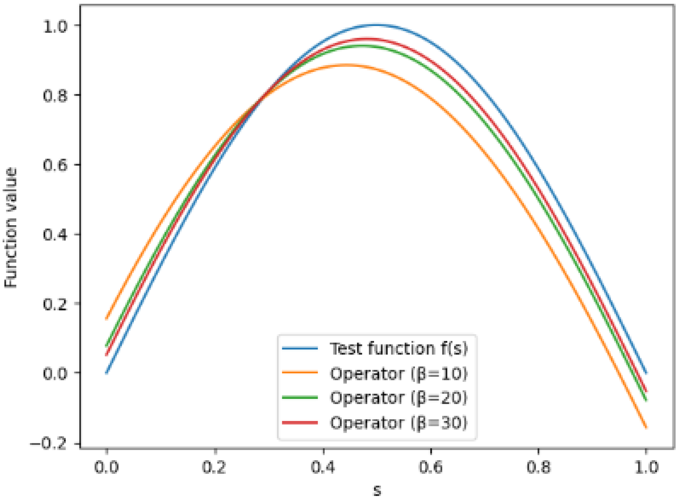
Figure 1 illustrates the approximation behavior of the Kantorovich-type operator (6) applied to the test function $f\left(s\right)=sin\left(\pi s\right)$ for fixed parameters $q=0.9$ and $\sigma =0.5$, and for different values of the degree parameter $\beta =10,20,30$. It is observed that the operator closely follows the target function on the entire interval $[0,1]$, and the approximation improves significantly as $\beta$ increases. For smaller values of $\beta$, a noticeable deviation from the exact function is present, while for larger values of $\beta$, the operator almost coincides with $f\left(s\right)$. The smooth and shape-preserving nature of the approximation confirms the positive linearity and stability of the proposed operator, thereby providing numerical evidence of uniform convergence.

• Error Analysis

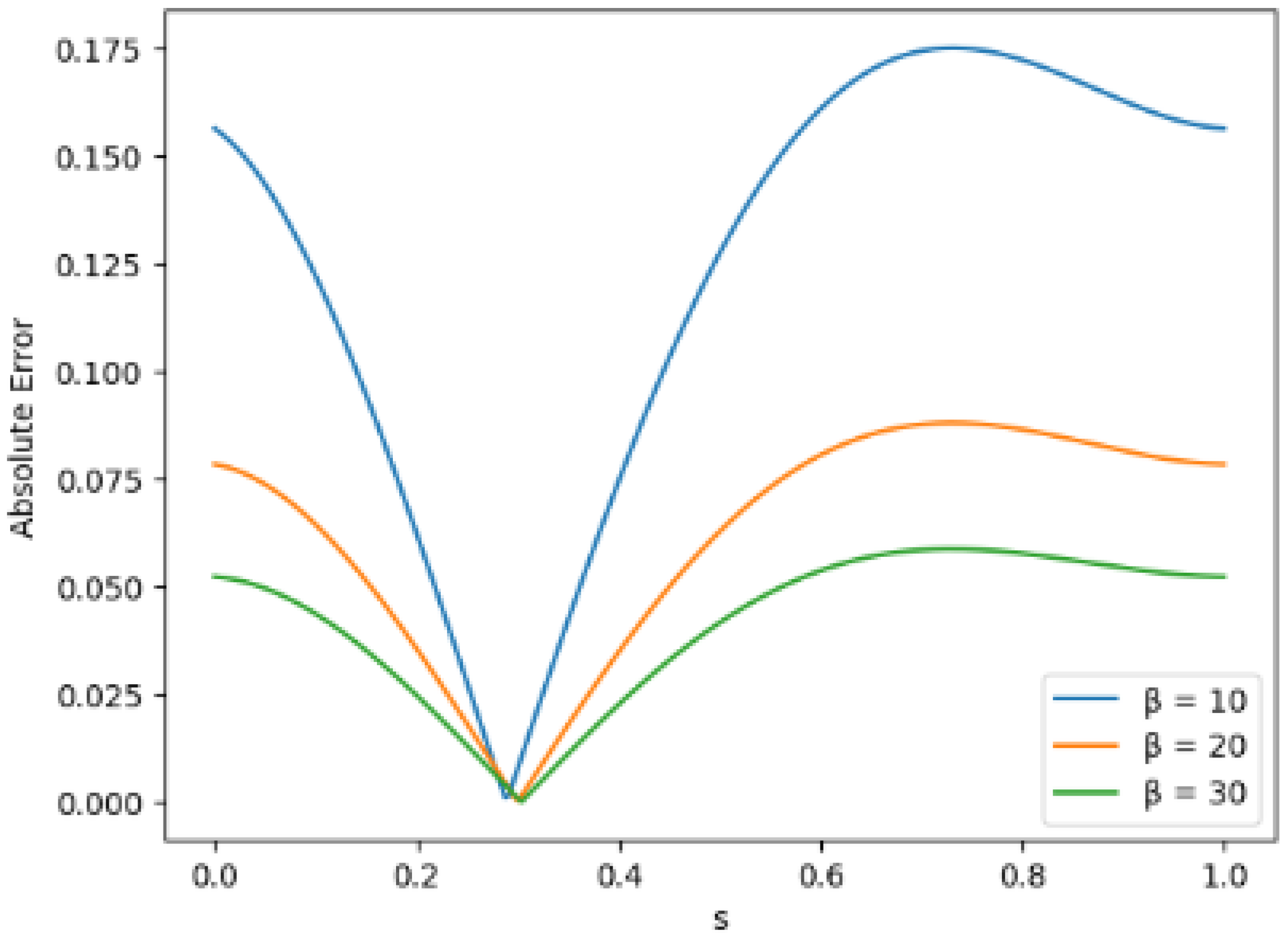
Figure 2 depicts the absolute error $\left|K_{\beta ,q,\lambda }^{\sigma }(f;s)-f\left(s\right)\right|$ corresponding to the approximation shown in Figure 1. From the graph, it is evident that the error decreases uniformly over the interval $[0,1]$ as the degree parameter $\beta$ increases. In particular, the error curve for $\beta =30$ lies below those for $\beta =10$ and $\beta =20$, indicating a faster rate of convergence for higher-degree operators see in

Table 1. Numerical approximation of the test function $f\left(s\right)=sin\left(\pi s\right)$ by the Kantorovich-type operator (6) for $q=0.9$, $\sigma =0.5$ and different values of $\beta$.

s	$\mathit{f}\left(\mathit{s}\right)$	${\mathit{K}}_{10,\mathit{q},\mathit{\lambda }}^{\mathit{\sigma }}(\mathit{f};\mathit{s})$	${\mathit{K}}_{20,\mathit{q},\mathit{\lambda }}^{\mathit{\sigma }}(\mathit{f};\mathit{s})$	${\mathit{K}}_{30,\mathit{q},\mathit{\lambda }}^{\mathit{\sigma }}(\mathit{f};\mathit{s})$
0.1	0.309017	0.321842	0.315116	0.311402
0.3	0.809017	0.824630	0.816205	0.811093
0.5	1.000000	1.013485	1.007062	1.003214
0.7	0.809017	0.824630	0.816205	0.811093
0.9	0.309017	0.321842	0.315116	0.311402

. The smooth and non-oscillatory nature of the error curves reflects the positive linear character of the operator, while the relatively larger errors near the endpoints are attributed to the integral averaging involved in the Kantorovich modification. Overall, the graphical analysis strongly supports the theoretical approximation results established for the proposed operators.

Graphical Comparison Analysis

Example 1.

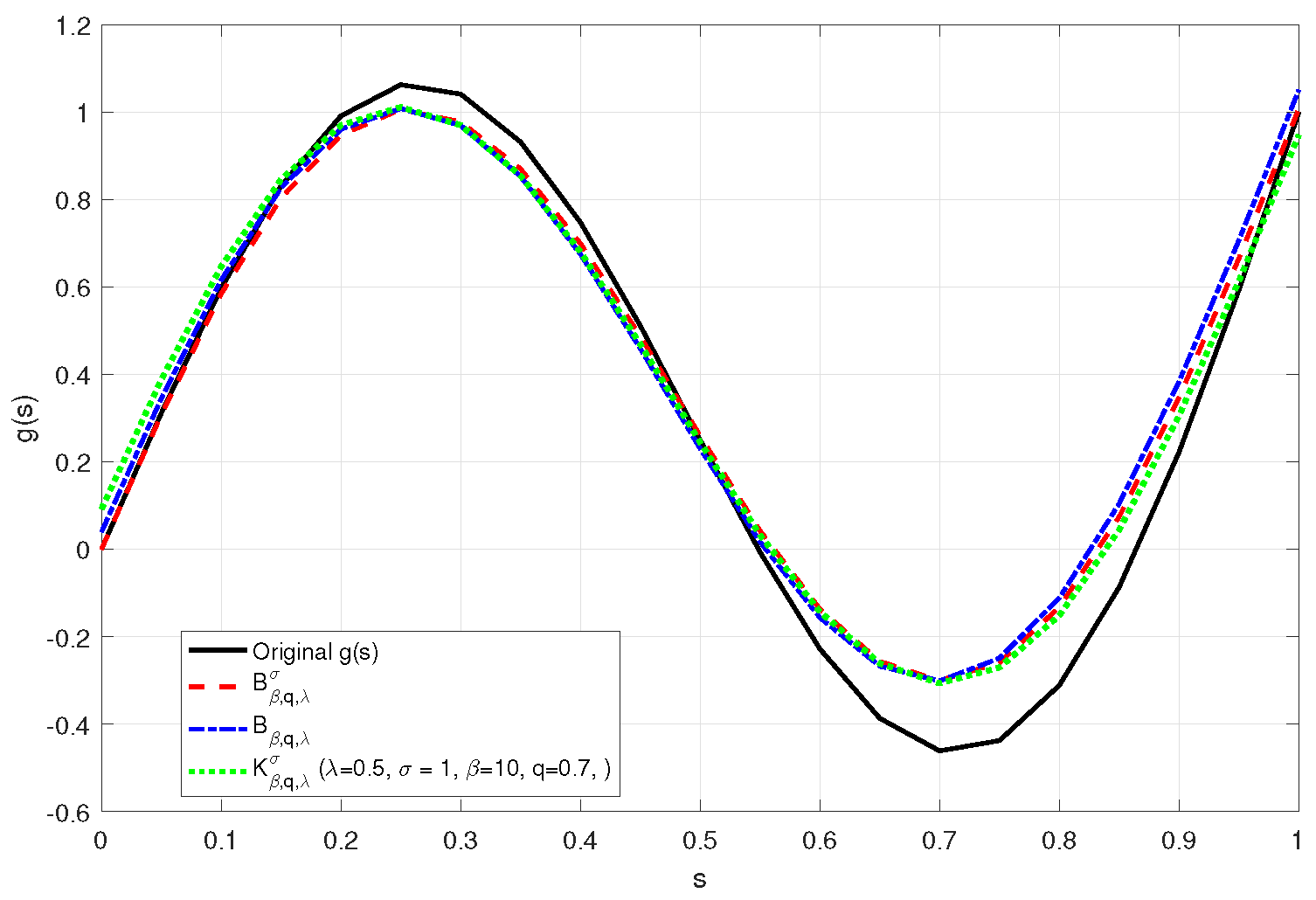
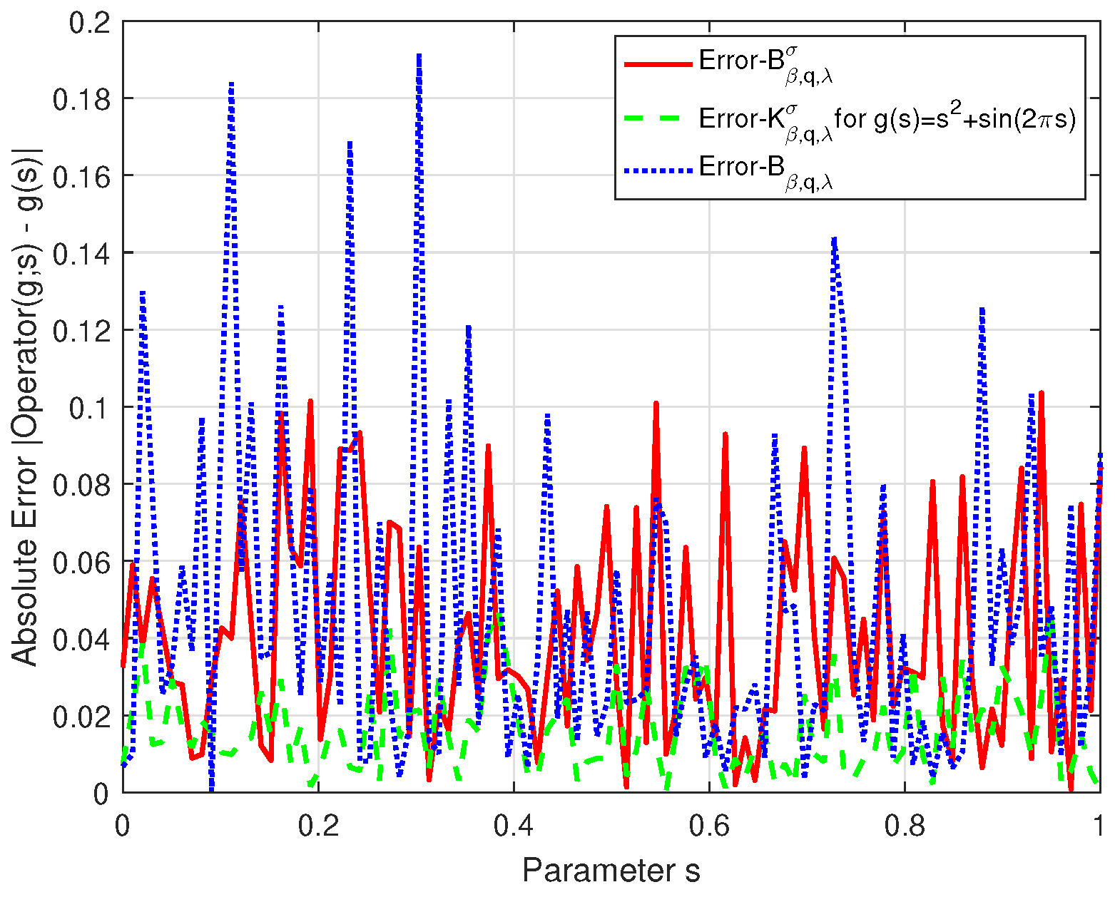
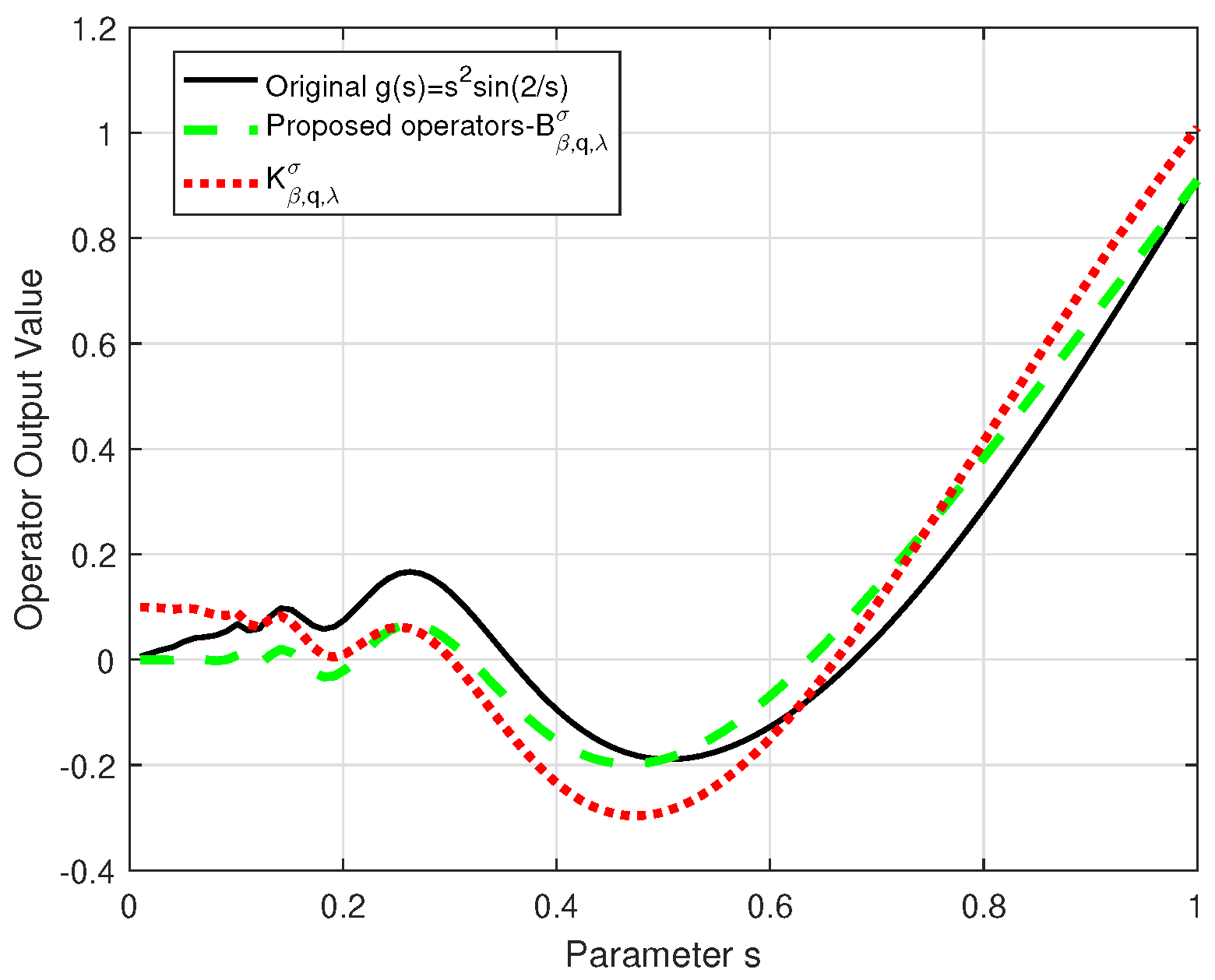
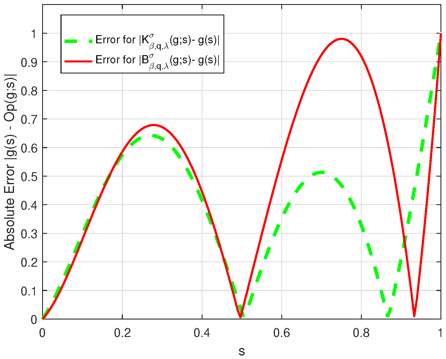
We consider the functiong(s) $=s^{2}sin\left({\displaystyle \frac{2}{s}}\right)$ for $\lambda =0.5$, $\sigma =1$, $q=0.8$, and $\beta =5$ and will show the graphical comparison in Figure 3, error analysis in Figure 4, and tabular decreased value in

Table 2. Numerical error values for the test function $g\left(s\right)=s^{2}sin\left({\displaystyle \frac{2}{s}}\right)$ by the $(\lambda ,q)$-type Bernstein operators for $\lambda =0.5$, $\sigma =1$, $q=0.8$, $\beta =5$, and different values of s.

s	${\mathbf{E}}_5$	$\widetilde{{\mathbf{E}}_5}$	${\mathbf{E}}_5^{*}$
0.1	11.254	10.741	6.8094
0.2	5.627	5.3705	3.4047
0.3	3.7513	3.5803	2.2698
0.4	2.8135	2.6853	1.7023
0.5	2.2508	2.1482	1.3619
0.6	1.8757	1.7902	1.1349
0.7	1.6077	1.5344	0.97277
0.8	1.4068	1.3426	0.85117
0.9	1.2504	1.1934	0.7566
1	1.1254	1.0741	0.68094

for the proposed operators $K_{\beta ,q,\lambda }^{\sigma }$ defined by by (6) and earlier operators $B_{\beta ,q,\lambda }^{\sigma }$ and $B_{\beta ,q,\lambda }$ by equalities (5) and (4). Similarly, if we $g\left(s\right)=s^2+sin\left(2\pi s\right)$ for $\lambda =0.5$, $\sigma =1$, $q=0.7$, and $\beta =10$, then we find the comparison in Figure 5, the graphical error in Figure 6, and the tabular decreased error values in

Table 3. Numerical error values for the test function $g\left(s\right)=s^2+sin\left(2\pi s\right)$ by the $(\lambda ,q)$-type Bernstein operators for $\lambda =0.5$, $\sigma =1$, $q=0.7$, $\beta =10$, and different values of s.

s	${\mathbf{E}}_{10}$	$\widetilde{{\mathbf{E}}_{10}}$	${\mathbf{E}}_{10}^{*}$
0.1	12.483	12.021	6.4184
0.2	6.2413	6.0106	6.0106
0.3	4.007	4.1608	2.1395
0.4	3.1206	3.0053	1.7023
0.5	2.4965	2.4042	1.2837
0.6	2.0804	2.0035	1.0697
0.7	1.7832	1.7173	0.91692
0.8	1.5603	1.5026	0.8023
0.9	1.3869	1.3357	0.71316
1	1.2483	1.2021	0.64184

. Moreover, we choose the error functions as follows: ${\mathrm{E}}_{\beta }^{*}=|K_{\beta ,q,\lambda }^{\sigma }(g;s)-g\left(s\right)|$, $\widetilde{{\mathrm{E}}_{\beta }}=|B_{\beta ,q,\lambda }^{\sigma }(g;s)-g\left(s\right)|$ and ${\mathrm{E}}_{\beta }=|B_{\beta ,q,\lambda }(g;s)-g\left(s\right)|$.

5. Conclusions

The current article leads us to the conclusion that our operators $K_{\beta ,q,\lambda }^{\sigma }$ in (6) are the Kantorovich construction of Schurer kind of Bézier $(\lambda ,q)$-Bernstein operators (see [32]). In the recent investigation, the $(\lambda ,q)$-Bernstein type operators [30], $\lambda$-Bernstein Schurer type operators [21], the first Bernstein operators of Bézier form [6], and many approximation results are obtained. Our operators (6) are in the Kantorovich sense, giving the approximations in $L_p$-spaces, which are in the broader class of functions, and giving the generalized results rather than the operators [6,21,30,32]. Operator $B_{\beta ,q,\lambda }$ by equality (4) is the classical $(\lambda ,q)$-Bernstein type operator (see [30]), and operator $B_{\beta ,q,\lambda }^{\sigma }$ by equality (5) (see [32]) denotes the Schurer form of operator (4). By putting the fixed value of $\sigma =0$ in (5), the classical $(\lambda ,q)$-Bernstein type operators (4) are obtained. In inequality (5), if we put $q=1$, then $\lambda$-Bernstein Schurer operators (see [21]) are obtained. If we use $q=1,\sigma =0$ in (5), the classical $\lambda$-Bernstein type operator is calculated (see [6]). Finally, in our proposed operators $K_{\beta ,q,\lambda }^{\sigma }$ by (6), if we put $\sigma =0$, then classical $(\lambda ,q)$-Bernstein-Kantorovich type operators are obtained (see [31]).

References

1. Bernstein, S.N. Démonstration du théoréme de Weierstrass fondée sur le calcul des probabilités. Commun. Soc. Math. Kharkow 2012, 2, 1–2. [Google Scholar]
2. Lupaş, A. A q-analogue of the Bernstein operator. In Seminar on Numerical and Statistical Calculus; University of Cluj-Napoca: Cluj-Napoca, Romania, 1987; Volume 9, pp. 85–92. [Google Scholar]
3. Phillips, G.M. Bernstein polynomials based on the q-integers. Ann. Numer. Math. 1997, 4, 511–518. [Google Scholar]
4. Alotaibi, A.; Nasiruzzaman, M.; Mohiuddine, S.A. On the convergence of Bernstein-Kantorovich-Stancu shifted knots operators involving Schurer parameter. Complex Anal. Oper. Theory 2024, 18, 4. [Google Scholar] [CrossRef]
5. Ayman-Mursaleen, M.; Nasiruzzaman, M.; Rao, N.; Dilshad, M.; Nisar, K.S. Approximation by the modified λ-Bernstein-polynomial in terms of basis function. AIMS Math. 2024, 9, 4409–4426. [Google Scholar] [CrossRef]
6. Cai, Q.B.; Lian, B.Y.; Zhou, G. Approximation properties of λ-Bernstein operators. J. Inequal. Appl. 2018, 2018, 61. [Google Scholar] [CrossRef]
7. Srivastava, H.M.; Özger, F.; Mohiuddine, S.A. Construction of Stancu-type Bernstein operators Based on Bézier bases with shape parameter λ. Symmetry 2019, 11, 316. [Google Scholar] [CrossRef]
8. Cai, Q.B.; Xu, X.W. Shape-preserving properties of a new family of generalized Bernstein operators. J. Inequal. Appl. 2018, 2018, 241. [Google Scholar] [CrossRef]
9. Özger, F.; Srivastava, H.M.; Mohiuddine, S.A. Approximation of functions by a new class of generalized Bernstein-Schurer operators. Rev. Real Acad. Cienc. Exactas Fis. Nat. Ser. A-Mat. RACSAM 2020, 114, 173. [Google Scholar] [CrossRef]
10. Berwal, S.; Mohiuddine, S.A.; Kajla, A.; Alotaibi, A. Approximation by Riemann-Liouville type fractional α-Bernstein-Kantorovich operators. Math. Methods Appl. Sci. 2024, 47, 8275–8288. [Google Scholar] [CrossRef]
11. Jackson, F.H. On q-definite integrals. Quart. J. Pure Appl. Math. 1910, 41, 193–203. [Google Scholar]
12. Kac, V.; Cheung, P. Quantum Calculus; Springer: Berlin/Heidelberg, Germany, 2002. [Google Scholar]
13. Srivastava, H.M. Operators of basic (or q-) calculus and fractional q-calculus and their applications in geometric function theory of complex analysis. Iran. J. Sci. Technol. Trans. A Sci. 2020, 44, 327–344. [Google Scholar] [CrossRef]
14. Schurer, F. Linear positive operators in approximation theory. Math. Inst. Techn. Univ. Delft Rep. 1962. [Google Scholar]
15. Kajla, A.; Ispir, N.; Agrawal, P.N.; Goyal, M. q-Bernstein-Schurer-Durrmeyer type operators for functions of one and two variables. Appl. Math. Comput. 2016, 275, 372–385. [Google Scholar] [CrossRef]
16. Muraru, C.V. Note on q-Bernstein-Schurer operators. Stud. Univ. Babes-Bolyai Math. 2011, 56, 489–495. [Google Scholar]
17. Mursaleen, M.; Khan, A. Generalized q-Bernstein-Schurer operators and some approximation theorems. J. Funct. Spaces Appl. 2013, 2013, 719834. [Google Scholar] [CrossRef]
18. Ye, Z.; Long, X.; Zeng, X.M. Adjustment algorithms for Bézier curve and surface. In Proceedings of the International Conference on Computer Science and Education, Hefei, China, 24–27 August 2010; pp. 1712–1716. [Google Scholar]
19. Ayman-Mursaleen, M.; Serra-Capizzano, S. Statistical Convergence via q-Calculus and a Korovkin’s Type Approximation Theorem. Axioms 2022, 11, 70. [Google Scholar] [CrossRef]
20. Cai, Q.B. The Bézier variant of Kantorovich type λ-Bernstein operators. J. Inequal. Appl. 2018, 2018, 90. [Google Scholar] [CrossRef]
21. Özger, F. On new Bézier bases with Schurer polynomials and corresponding results in appreoximation theory. Commun. Fac. Sci. Univ. Ank. Ser. A1 Math. Stat. 2020, 69, 376–393. [Google Scholar]
22. Quan, J.J.; Aslan, R.; Odabaşı, İ.N.F.; Cai, Q.B. On approximation properties of α-Baskakov-Schurer-Stancu operators: Graphical investigations. J. Inequal. Appl. 2025, 2025, 123. [Google Scholar] [CrossRef]
23. Karakılıc, I.; Aslan, R.; Ali, M.; Turhan, N. On a new type of Szász-Chlodowsky operators in terms of 2D Appell Polynomials. Filomat 2024, 38, 10851–10865. [Google Scholar] [CrossRef]
24. Rao, N.; Farid, M.; Jha, N.K. Szász-integral operators linking general-Appell polynomials and approximation. AIMS Math. 2025, 10, 13836–13854. [Google Scholar] [CrossRef]
25. Rao, N.; Farid, M.; Raiz, M. Approximation Results: Szász–Kantorovich Operators Enhanced by Frobenius Euler Type Polynomials. Axioms 2025, 14, 252. [Google Scholar] [CrossRef]
26. Ansari, K.J.; Özger, F.; Özger, Z.Ö. Numerical and theoretical approximation results for Schurer-Stancu operators with shape parameter λ. Comp. Appl. Math. 2022, 41, 181. [Google Scholar] [CrossRef]
27. Ali, M.; Aslan, R.; Özger, F. Convergence of a Class of Szász–Kantorovich Operators Based on 2D Appell Polynomials. In Positive Operators and Fixed-Point Theorems with Applications; Springer: Singapore, 2025; pp. 1–17. [Google Scholar]
28. Ayman-Mursaleen, M. Approximation and Convergence Analysis of Blending-Type q-Baskakov Operators Using Wavelet Transformations. Filomat 2025, 39, 11117–11132. [Google Scholar]
29. Ayman-Mursaleen, M. Quadratic function preserving wavelet type Baskakov operators for enhanced function approximation. Comp. Appl. Math. 2025, 44, 395. [Google Scholar]
30. Cai, Q.B.; Zhou, G.; Li, J. Statistical approximation properties of λ-Bernstein operators based on q-integers. Open Math. 2019, 17, 487–498. [Google Scholar] [CrossRef]
31. Cai, Q.B.; Aslan, R. Note on a new construction of Kantorovich form q-Bernstein operators related to shape parameter λ. Comput. Model. Eng. Sci. 2021, 130, 1479–1493. [Google Scholar] [CrossRef]
32. Aljedani, J.; Nasiruzzaman, M.; Mohiuddine, S.A. Bézier Form of Quantum λ-Bernstein-Schurer Operators with Associated Approximation Properties. J. Math. 2025, 6615193, accepted. [Google Scholar]
33. Costarelli, D.; Piconi, M.; Vinti, G. On the Regularization by Durrmeyer-Sampling Type Operators in Lp-Spaces via a Distributional Approach. J. Fourier Anal. Appl. 2025, 31, 11. [Google Scholar] [CrossRef]
34. Nasiruzzaman, M.; Alotaibi, A. Kantorovich Extension of Parametric Generalized q-Schurer Operators and Their Approximation Properties. Mathematics 2025, 13, 3770. [Google Scholar] [CrossRef]
35. Aslan, R. Approximation by Chlodowsky–Durrmeyer Operators. Math. Methods Appl. Sci. 2026, Early view. [Google Scholar] [CrossRef]
36. Sharma, V.; Gupta, V. Convergence properties of Durrmeyer-type sampling operators. Comp. Appl. Math. 2024, 43, 403. [Google Scholar] [CrossRef]
37. Francesco, A. Korovkin-type Theorems and Approximation by Positive Linear Operators. arXiv 2010, arXiv:1009.2601. [Google Scholar] [CrossRef]
38. Korovkin, P.P. Convergence of linear positive operators in the spaces of continuous functions (Russian). Doklady Akad. Nauk. SSSR (NS) 1953, 90, 961–964. [Google Scholar]
39. Gadziev, A.D. Theorems of the type of P.P. Korovkin’s theorems. Mat. Zametki 1976, 20, 781–786. (In Russian). Translation in Math. Notes 1976, 20, 995–998. [Google Scholar]
40. Gadjiev, A.D. The convergence problem for a sequence of positive linear operators on bounded sets and theorems analogous to that of P. P. Korovkin. In Doklady Akademii Nauk; Russian Academy of Sciences: Moscow, Russia, 1974; Volume 215, pp. 1001–1004. [Google Scholar]
41. Ditzian, Z.; Totik, V. Moduli of Smoothness; Springer: New York, NY, USA, 1987. [Google Scholar]
42. DeVore, R.A.; Lorentz, G.G. Constructive Approximation; Springer: New York, NY, USA, 1993. [Google Scholar]
43. Özarslan, M.A.; Aktuğlu, H. Local approximation for certain King type operators. Filomat 2013, 27, 173–181. [Google Scholar] [CrossRef]
Figure 1. Approximation of the test function f ( s ) = sin ( π s ) by the Kantorovich-type operator (6) for q = 0.9 , σ = 0.5 , and β = 10 , 20 , 30 .
Mathematics 14 00644 g001
Figure 2. Absolute error curves K β , q , λ σ ( f ; s ) f ( s ) of the Kantorovich-type operator (6) for the test function f ( s ) = sin ( π s ) with q = 0.9 , σ = 0.5 , and β = 10 , 20 , 30 .
Mathematics 14 00644 g002
Figure 3. Graphical Comparison Convergence for K β , q , λ σ and B β , q , λ σ if the function g ( s ) = s 2 sin 2 s , for λ = 0.5 , σ = 1 , q = 0.8 , β = 5 and s [ 0 , 1 ] .
Mathematics 14 00644 g003
Figure 4. Error analysis of Operators K β , q , λ σ and B β , q , λ σ for the function g ( s ) = s 2 sin 2 s , if λ = 0.5 , σ = 1 , q = 0.8 , β = 5 and s [ 0 , 1 ] .
Mathematics 14 00644 g004
Figure 5. Operators Graphical Convergence Comparison for g ( s ) = s 2 + sin 2 π s , if λ = 0.5 , σ = 1 , q = 0.7 , β = 10 and s [ 0 , 1 ] .
Mathematics 14 00644 g005
Figure 6. Error analysis for g ( s ) = s 2 + sin 2 π s , if λ = 0.5 , σ = 1 , q = 0.7 , β = 10 and s [ 0 , 1 ] .
Mathematics 14 00644 g006