Computational Linearization of Nonlinear Kolmogorov Equations via the Generalized Newton Method in LSV Models

Abstract

This study develops a generalized Newton method to address the nonlinear Kolmogorov forward equation (KFE) under the local stochastic volatility (LSV) framework. Analytical convergence conditions are derived via the geometric series theorem, and empirical validation is conducted using 15 years of monthly crude oil spot price data (2011–2025), with the parameters set using maximum likelihood estimation. Sensitivity analyses confirm the stable convergence of the iterative scheme under realistic scenarios while also identifying parameter ranges that may lead to divergence. These findings demonstrate that the proposed methodology provides a tractable and accurate approach to probability density estimation in commodity markets, with a clear potential for extension to multi-dimensional settings and richer datasets.

1. Introduction

Stochastic volatility models have become a cornerstone of modern mathematical finance, providing more realistic dynamics for asset prices compared with classical constant-volatility frameworks. The seminal Heston model [1] introduced closed-form solutions for options under stochastic volatility and has since inspired extensive research. Empirical studies such as the work of Bakshi, Cao, and Chen [2] confirmed that stochastic volatility models often outperform traditional approaches, motivating the further exploration of nonlinear PDE formulations and calibration techniques. These models are particularly relevant for option pricing, risk management, and portfolio optimization, where capturing the joint behavior of asset prices and volatility is essential.

In particular, long-dated derivatives play a crucial role in energy and commodity markets. They are widely used for hedging long-term risks, managing exposure to volatility, and pricing contracts such as long-term options and swaps. These instruments provide market participants with the tools to stabilize revenue and mitigate uncertainty over extended time periods. In this context, our study highlights the practical relevance of the proposed methodology, as the accurate estimation of probability densities directly impacts the valuation and risk management of such long-term financial products. In this study, the term long-dated derivative refers to contracts that can be interpreted either as (i) options—long- or short-dated—written on long-term futures or (ii) long-term options written directly on the spot asset. This delineation ensures consistency with the standard market structures observed in energy and commodity markets.

Several numerical methods have been proposed to address nonlinear PDEs in finance. Duris [3] introduced linearization schemes for nonlinear Black–Scholes equations, while Rafael et al. [4] analyzed illiquid market effects. Mashayekhi [5] applied ADE methods to the Barles–Soner model, and Heider [6] demonstrated implicit schemes ensuring convergence. Within the stochastic local volatility (SLV) framework, Cui et al. [7] developed a general option valuation approach, and Saporito et al. [8] proposed calibration techniques. Guerrero et al. [9] extended local stochastic volatility (LSV) models to time-dependent settings, solvable using advanced PDE methods.

Despite these advances, solving the nonlinear Kolmogorov forward equation for local stochastic volatility (LSV) models remains analytically intractable. Moreover, existing numerical schemes—such as finite difference discretizations, implicit schemes, and ADE-based approaches—often suffer from slow convergence, sensitivity to initial conditions, or instability when the Jacobian matrix approaches singularity. To address these limitations, this study applies a generalized Newton method to linearize the equation. The proposed approach offers faster convergence, improved numerical stability, and a reduced dependence on initial guesses compared with classical iterative techniques. We analyze the existence, boundedness, and convergence via the geometric series theorem and illustrate the methodology with monthly crude oil price data, estimating unknown parameters and computing the risk-neutral probability density function of asset prices. The empirical example is based on a limited dataset and is presented only as a demonstration of the method’s feasibility.

1.1. Related Work

Beyond the directly related studies, the broader literature has explored stochastic volatility and nonlinear PDEs. Fouque et al. [10] provided a comprehensive reference on derivatives markets under stochastic volatility. Cont and Tankov [11] introduced jump processes to capture sudden market moves. Saheya et al. [12] proposed rational approximation models and improved Newton’s methods, while Antoni [13] refined Newton techniques for scalar nonlinear equations. Shehzad et al. [14] combined stochastic models with technical analysis for stock price prediction. Arregi et al. [15] studied PDE models for XVA and counterparty risk. Wallin et al. [16] developed PDE filtering methods, and Boussange et al. [17] compared machine learning and Picard iterations for non-local PDEs. Glaue et al. [18] formalized deep parametric PDE methods, while Mesgarani et al. [19] analyzed fractional Black–Scholes models with Caputo derivatives.

These contributions, while not directly addressing the Kolmogorov forward equation for local stochastic volatility (LSV) models, provide a valuable context and highlight the diversity of approaches in stochastic volatility modeling and nonlinear PDE analysis.

1.2. Arbitrage Considerations

Local stochastic volatility (LSV) models are not automatically arbitrage-free unless additional structural assumptions are imposed. In this paper, our objective is not to construct a fully tradable market model but rather to analyze the nonlinear Kolmogorov forward equation associated with a given diffusion specification. Following standard practice in the LSV literature, we work under the risk-neutral measure by fixing the drift of the asset price to the interest rate r, and we assume that the functions $a(t,S)$, $b\left(Y\right)$, and $\alpha (t,Y)$ satisfy Lipschitz continuity and linear-growth conditions. These assumptions ensure the existence of a unique weak solution to the SDE system and guarantee that the corresponding probability density is well-defined, which is sufficient for the purposes of our convergence analysis and numerical study.

The structure of this article is as follows: First, we introduce the local stochastic volatility (LSV) model and derive the Kolmogorov forward equation in both two- and general n-dimensional settings. Then, we apply the generalized Newton method to linearize the nonlinear Kolmogorov equation and establish analytical convergence conditions using the geometric series theorem. Next, we present the numerical implementation based on 15 years of monthly crude oil spot price data (2011–2025), where the model parameters are statistically estimated via maximum likelihood estimation, and the iterative solution is analyzed using sensitivity tests. Finally, we report the convergence behavior under realistic scenarios, identify parameter ranges that may lead to divergence, and outline the methodological implications and potential extensions to multi-dimensional models and richer datasets.

1.3. Introduction to the LSV Model

The local stochastic volatility (LSV) model, an extension of Dupire’s local volatility framework, is formulated through diffusion equations. In a two-dimensional setting, the dynamics of the LSV model can be expressed by the following system of stochastic differential equations (SDEs) (see [20]):

$$\begin{array}{c}\hfill \begin{array}{cc}\hfill & {\displaystyle \frac{d{S}_t}{S_t}}=a(t,S_t)b\left(Y_t\right)d{B}_t^1+rdt,\hfill \\ \hfill & d{Y}_t=\alpha (t,Y_t)d{B}_t^2+\xi \left(t\right)dt.\hfill \end{array}\end{array}$$

(1)

Here, the asset price process is denoted by $(S_t,t\ge 0)$, and the stochastic component of volatility is represented by $(Y_t,t\ge 0)$. The function b maps this component to an effective volatility measure. The parameter a captures the local volatility aspect of the model, allowing calibration to vanilla option prices. The volatility of the volatility is denoted by $\alpha$, while r and $\xi$ represent drift terms that may depend on the time and state variables. The model incorporates two Brownian motions, $B^1$ and $B^2$, with the correlation coefficient $\rho$, which is assumed to be constant here, as a simplifying assumption.

We impose standard Lipschitz continuity and linear-growth conditions on the coefficient functions a, b, $\alpha$, and $\xi$, ensuring the existence and uniqueness of solutions to the SDE system. These assumptions also guarantee sufficient regularity of the associated Kolmogorov forward equations, providing a consistent mathematical foundation for subsequent analysis and applications in option pricing and risk management.

1.3.1. Kolmogorov Forward Equation Derivation

To align with the model’s assumptions, we derive the Kolmogorov forward equation for the joint probability density function, $p(t,s,y)$, of the stock price process $(S_t,t\ge 0)$ and the stochastic volatility process $(Y_t,t\ge 0)$:

$$\begin{array}{c}\hfill \begin{array}{cc}\hfill & {\displaystyle \frac{\partial p}{\partial t}}-{\displaystyle \frac{{\partial }^{2}p}{\partial S^2}}\left(\frac{1}{2}{a}^2{b}^2{S}^2\right)-{\displaystyle \frac{{\partial }^{2}p}{\partial S\partial y}}\left(\rho ab\alpha S\right)-{\displaystyle \frac{{\partial }^{2}p}{\partial y^2}}\left(\frac{1}{2}{\alpha }^2\right)\hfill \\ \hfill & +{\displaystyle \frac{\partial p}{\partial S}}\left(rS\right)+{\displaystyle \frac{\partial p}{\partial y}}\xi +rp=0,\hfill \\ \hfill & p(S,y,0)=\delta (S=S_0,y=y_0).\hfill \end{array}\end{array}$$

(2)

Under the stated regularity and growth assumptions, Equation (2) is valid. Given the initial conditions $(S_0,y_0)$, the marginal density of the stock price, $q(t,s)$, is obtained by integrating the joint probability density function $p(t,s,y)$ with respect to the stochastic volatility component y:

$$q(t,s)=\int p(t,s,y)dy.$$

$$\begin{array}{c}\hfill \begin{array}{c}\hfill {\displaystyle \frac{\partial q}{\partial t}}-{\displaystyle \frac{{\partial }^2}{\partial S^2}}\left(\frac{1}{2}{a}^2{S}^2\left(\int b^{2}pdy\right)\right)+{\displaystyle \frac{\partial }{\partial S}}\left(rSq\right)+rq=0.\end{array}\end{array}$$

(3)

This marginal density connects the probabilistic formulation of the model with market-observed vanilla option prices, providing the basis for calibration. Based on Dupire’s findings [21], the marginal density of the stock price $q(t,s)$ must satisfy

$$\begin{array}{c}\hfill \begin{array}{c}\hfill {\displaystyle \frac{\partial q}{\partial t}}-{\displaystyle \frac{{\partial }^2}{\partial S^2}}\left(\frac{1}{2}{\sigma }_D^2{S}^{2}q\right)+{\displaystyle \frac{\partial }{\partial S}}\left(rSq\right)+rq=0.\end{array}\end{array}$$

(4)

Dupire’s local volatility, denoted by ${\sigma }_D$, is inferred from the observed vanilla option prices. In our numerical illustration, we rely on a limited dataset of monthly crude oil prices, which serves only to demonstrate the feasibility. A more extensive dataset would be required for robust empirical validation.

$$a^2(t,S)={\sigma }_D^2(t,S){\displaystyle \frac{\int pdy}{\int b^{2}pdy}}.$$

The primary objective is to determine the joint density function $p(t,s,y)$ that captures the observed market dynamics. This joint density is obtained as the solution to a nonlinear partial integro-differential equation (see [20]):

$$\begin{array}{c}\hfill \begin{array}{cc}\hfill & {\displaystyle \frac{\partial p}{\partial t}}-{\displaystyle \frac{{\partial }^{2}p}{\partial S^2}}\left(\frac{1}{2}{\sigma }_D^2{b}^2{S}^2{\displaystyle \frac{\int pdy}{\int b^{2}pdy}}\right)-{\displaystyle \frac{{\partial }^{2}p}{\partial S\partial y}}\left(\rho {\sigma }_{D}b\alpha S{\left({\displaystyle \frac{\int pdy}{\int b^{2}pdy}}\right)}^{1/2}\right)\hfill \\ \hfill & -{\displaystyle \frac{{\partial }^{2}p}{\partial y^2}}\left(\frac{1}{2}{\alpha }^2\right)+{\displaystyle \frac{\partial p}{\partial S}}\left(rS\right)+{\displaystyle \frac{\partial p}{\partial y}}\xi +rp=0.\hfill \end{array}\end{array}$$

(5)

Equation (5) defines a nonlinear partial integro-differential equation whose solution yields the joint density $p(t,s,y)$. In this study, we focus on illustrating the methodology with simplified assumptions. Future work will include quantitative error analysis and calibration with larger datasets to assess the robustness.

1.3.2. Multi-Dimensional Problem Formulation

Let $\{0\le t\le T\}$ represent time, and let $x=(x_1,x_2,\dots ,x_n)\in \Omega \subset {\mathbb{R}}^n$ denote the spatial variable, where $\Omega$ is a bounded domain in ${\mathbb{R}}^n$ with a sufficiently smooth boundary. In financial applications, $x_1$ represents the stock price $\left(S\right)$, while the remaining $n-1$ components of x represent the volatility factors. We define $D^T=[0,T]\times \Omega$ as the space–time domain, with $B=\left\{0\right\}\times \Omega$ representing the initial boundary, $B^T=\left\{T\right\}\times \Omega$ representing the terminal boundary, and $C^T=[0,T]\times \partial \Omega$ representing the lateral boundary.

Furthermore, we define ${\Omega }_S=\{S\in \mathbb{R}\mid \exists y\in {\mathbb{R}}^{n-1},(S,y)\in \Omega \}$ as the set of admissible stock prices, and for each $S\in {\Omega }_S$, we define ${\Omega }_y^S=\{y\in {\mathbb{R}}^{n-1},(S,y)\in \Omega \}$ as the set of admissible volatility factors for a given stock price. Our primary focus is on the following equation:

$$\begin{array}{c}\hfill \begin{array}{cc}\hfill F\left(p\right):=& {\displaystyle \frac{\partial p}{\partial t}}-{\displaystyle \frac{{\partial }^{2}p}{\partial S^2}}\left({\rho }_{11}{\alpha }_1^{2}I\left(p\right)\right)-\sum _{i=2}^n{\displaystyle \frac{{\partial }^{2}p}{\partial S\partial x_i}}\left({\rho }_{1i}{\alpha }_1{\alpha }_i\sqrt{I\left(p\right)}\right)\hfill \\ \hfill & -\sum _{i,j=2}^n{\displaystyle \frac{{\partial }^{2}p}{\partial x_i\partial x_j}}\left({\rho }_{ij}{\alpha }_i{\alpha }_j\right)+\sum _{i=1}^n{\displaystyle \frac{\partial p}{\partial x_i}}{\beta }_i+\gamma p=0,\hfill \\ \hfill & \mathrm{on}{D}^T\cup B^T.\hfill \end{array}\end{array}$$

(6)

The correlation matrix, denoted by $\left({\rho }_{ij},1\le i,j\le n\right)$, is symmetric, positive definite, and satisfies the following illustrative conditions:

• ${\rho }_{ii}=\frac{1}{2}$ for all i (chosen here for analytical tractability);
• $-\frac{1}{2}\le {\rho }_{ij}\le \frac{1}{2}$ for $i\ne j$.

Fixing ${\rho }_{ii}=\frac{1}{2}$ is a simplifying assumption adopted for clarity. In practice, correlation and leverage effects play a crucial role in local stochastic volatility models, and empirical estimation or sensitivity analysis would be required for robust calibration. Extending the framework to empirically estimated correlation structures is left for future work.

We impose the boundary condition $p=\Psi$ on $\overline{B}\cup C^T$, where $\Psi$ is constant on $C^T$. The initial condition is defined as $p_0(t,S,y)=\Psi (S,y)$. The complexity of this equation stems from the presence of the integral term

$$\begin{array}{c}\hfill \begin{array}{cc}\hfill I\left(p\right)(t,s)=& {\displaystyle \frac{{\int }_{{\Omega }_y^s}p(t,s,x_2,\dots ,x_n)d{x}_2\dots d{x}_n}{{\int }_{{\Omega }_y^s}{b}^2(x_2,\dots ,x_n)p(t,s,x_2,\dots ,x_n)d{x}_2\dots d{x}_n}}\hfill \\ \hfill & ·{\displaystyle \frac{{\int }_{{\Omega }_y^s}p(t,s,y)dy}{{\int }_{{\Omega }_y^s}{b}^2\left(y\right)p(t,s,y)dy}}.\hfill \end{array}\end{array}$$

(7)

Equation (7) is classified as a nonlinear, parabolic, and non-local equation (see [20]). In this study, we focus on illustrating the methodology with simplified assumptions. A more rigorous empirical calibration and sensitivity analysis of the integral term will be necessary in future work to assess the robustness.

2. Linearization and Convergence Analysis

In this section, we employ the generalized Newton method to linearize the nonlinear Kolmogorov equation, which models local volatilities. We then analyze the convergence of the resulting linear system using the geometric series theorem, which provides conditions for the existence of a solution. Finally, we discuss the stability of the obtained solution within this framework.

2.1. Foundational Concepts: Fréchet Differentiability and Newton’s Method

We briefly recall the foundational concepts that underpin the linearization procedure. These definitions provide the functional analytic framework in which the generalized Newton method is applied to the nonlinear Kolmogorov operator.

Definition 1.

The operator F at $u_0$ is Fréchet differentiable if and only if there exists a bounded linear operator $A\in L(V,W)$ such that

$$f(u_0+h)=f\left(u_0\right)+Ah+o\left(\right|\left|h\right|\left|\right),h⟶0.$$

In this case, the operator F at $u_0$ is Fréchet differentiable, and we denote the Fréchet derivative of F at $u_0$ by $f^{\prime }\left(u_0\right)$ [22].

Remark 1.

Throughout this study, we assume that the nonlinear Kolmogorov operator

$$F:H^2(\Omega )⟶L^2(\Omega ),$$

where $\Omega \subset {\mathbb{R}}^n$ is a bounded domain with a sufficiently smooth boundary. This choice ensures that F acts on functions with square-integrable second derivatives, and its image lies in the Hilbert space $L^2(\Omega )$. Under these assumptions, the Fréchet differentiability of F is well-defined, and the boundedness of F, $F^{\prime }\left(p\right)$, and $F^{″}\left(p\right)$ can be rigorously interpreted in the operator norm of $L^2(\Omega )$. This functional setting provides the analytical foundation for applying the generalized Newton method and guarantees that the linearization procedure is valid within the Banach space framework.

Definition 2.

Suppose U and V are two Banach spaces, and $F:U⟶V$ is a differentiable function. We are interested in solving the following equation:

$$F\left(u\right)=0.$$

We compute the Newton iterates by choosing an initial guess $u_0\in U$, and then, for $n=0,1,2,\dots$, we iterate as follows [22]:

$$u_{n+1}=u_n-{\left[F^{\prime }\left(u_n\right)\right]}^{-1}F\left(u_n\right).$$

Remark 2.

In the present framework, we consider $U=H^2(\Omega )$, the Sobolev space of functions with square-integrable second derivatives on a bounded domain $\Omega \subset {\mathbb{R}}^n$ with a smooth boundary, and $V=L^2(\Omega )$. This setting ensures that F is well-defined as a nonlinear operator acting on sufficiently regular functions, and its Fréchet derivative $F^{\prime }\left(u\right)$ is a bounded linear operator from $H^2(\Omega )$ to $L^2(\Omega )$. These assumptions provide the functional analytic foundation for applying Newton’s method to the nonlinear Kolmogorov operator.

Definition 3.

We assume that $F:{\mathbb{R}}^d⟶{\mathbb{R}}^d$ is a continuously differentiable function. A system of nonlinear equations can be expressed in the following form [22]:

$$u\in {\mathbb{R}}^d,F\left(u\right)=0.$$

Newton’s method is expressed as

$$u_{n+1}=u_n-{\left[F^{\prime }\left(u_n\right)\right]}^{-1}F\left(u_n\right).$$

Furthermore, Newton’s method is often written as

$$F^{\prime }\left(u_n\right){\delta }_n=-F\left(u_n\right),{\delta }_n=u_{n+1}-u_n.$$

Remark 3.

In finite-dimensional settings, $F:{\mathbb{R}}^d\to {\mathbb{R}}^d$ is assumed to be continuously differentiable; therefore, $F^{\prime }\left(u_n\right)$ is represented by the Jacobian matrix of F at $u_n$. This corresponds to the operator framework introduced earlier, where, in infinite-dimensional cases, we considered $F:H^2(\Omega )\to L^2(\Omega )$. Thus, Definition 3 can be viewed as the finite-dimensional analogue of Newton’s method, with $F^{\prime }\left(u_n\right)$ acting as a bounded linear operator on ${\mathbb{R}}^d$. This connection clarifies that the iterative scheme is consistent across both Banach spaces and Euclidean settings.

In the context of our study, these definitions are applied to the nonlinear Kolmogorov operator introduced in Section 1.3.2. The Fréchet differentiability ensures that the operator admits a well-defined linearization, while Newton’s method provides an iterative scheme for approximating solutions. For clarity, we emphasize that the functional setting is assumed to be Banach spaces of sufficiently smooth functions (e.g., $C^2$ or Sobolev spaces $H^k$). Standard regularity and growth conditions on the coefficients guarantee the validity of these definitions in the present framework. A complete proof of convergence is beyond the scope of this paper and is left for future work.

2.2. Newton’s Method Application and Linearized Equation

In this segment, we extend the concept of real function derivatives to operators. We define an operator F by the following equation:

$$F\left(p\right)=0,$$

where F is given by Equation (6).

$$\begin{array}{c}\hfill \begin{array}{cc}\hfill F\left(p\right):=& p_t-p_{ss}\left({\rho }_{11}{\alpha }_1^{2}I\left(p\right)\right)-\sum _{i=2}^n{p}_{s{x}_i}\left({\rho }_{1i}{\alpha }_1{\alpha }_i\sqrt{I\left(p\right)}p\right)\hfill \\ \hfill & -\sum _{i,j=2}^n{p}_{x_i{x}_j}\left({\rho }_{ij}{\alpha }_i{\alpha }_j\right)+\sum _{i=1}^n{p}_{x_i}{\beta }_i+\gamma p=0.\hfill \end{array}\end{array}$$

(8)

According to Definitions 2 and 3, the Newton method for solving Equation (8) is as follows:

$$\begin{array}{c}\hfill \begin{array}{c}\hfill p_{n+1}=p_n-{\left[F^{\prime }\left(p_n\right)\right]}^{-1}F\left(p_n\right).\end{array}\end{array}$$

(9)

Alternatively, the iteration can be expressed as

$$\begin{array}{c}\hfill \begin{array}{c}\hfill F^{\prime }\left(p_n\right)(p_{n+1}-p_n)=-F\left(p_n\right).\end{array}\end{array}$$

(10)

We now calculate the Fréchet derivative of $F\left(p_n\right)$ using Definition 1 and Equation (8) (see [23] for further details):

$$\begin{array}{c}\hfill \begin{array}{cc}\hfill F^{\prime }\left(p_n\right)\left(\delta \right)\left(t\right)& =\underset{h\to 0}{lim}{\displaystyle \frac{1}{h}}[F(p+h\delta )\left(t\right)-F\left(p\right)\left(t\right)]\hfill \\ \hfill & =\underset{h\to 0}{lim}{\displaystyle \frac{1}{h}}[{\delta }_{t}h-{\delta }_{ss}h{\rho }_{11}{\alpha }_{11}^{2}I(p+\delta h)\hfill \\ \hfill & -\sum _{i=2}^{n}h{\delta }_{s{x}_i}\left({\rho }_{1i}{\alpha }_1{\alpha }_i\sqrt{I(p+\delta h)}\right)\hfill \\ \hfill & -\sum _{i,j=2}^{n}h{\delta }_{x_i{x}_j}\left({\rho }_{ij}{\alpha }_i{\alpha }_j\right)+\sum _{i=1}^{n}h{\delta }_{x_i}{\beta }_i+h\delta \gamma ].\hfill \end{array}\end{array}$$

(11)

As a result, the linearized form of the partial differential equation for the local stochastic volatility model is as follows (see Appendix A):

$$\begin{array}{c}\hfill \begin{array}{cc}\hfill F^{\prime }\left(p_n\right)\left(\delta \right)\left(t\right)& ={\delta }_t-{\delta }_{ss}{\rho }_{11}{\alpha }_{11}^{2}I\left(p\right)-\sum _{i=2}^n{\delta }_{s{x}_i}\left({\rho }_{1i}{\alpha }_1{\alpha }_i\sqrt{I\left(p\right)}\right)\hfill \\ \hfill & -\sum _{i,j=2}^n{\delta }_{x_i{x}_j}\left({\rho }_{ij}{\alpha }_i{\alpha }_j\right)+\sum _{i=1}^n{\delta }_{x_i}{\beta }_i+\gamma \delta .\hfill \end{array}\end{array}$$

(12)

Furthermore, we can employ Newton’s method to address this issue and additionally incorporate

$$\begin{array}{c}\hfill \begin{array}{c}\hfill {\delta }_n(s,t,y)=p_{n+1}(s,t,y)-p_n(s,t,y),n=0,1,2,\dots \end{array}\end{array}$$

(13)

Utilizing Equations (8) and (10)–(13), we establish the following relationships (see Appendix B):

$$\begin{array}{c}\hfill \begin{array}{cc}\hfill p(n+1)& ={\displaystyle \frac{1}{\gamma }}[-p_t(n+1)p_{ss}(n+1)\left({\rho }_{11}{\alpha }_{11}^{2}I\left(p_n\right)\right)\hfill \\ \hfill & +\sum _{i=2}^n{p}_{s{x}_i}(n+1)\left({\rho }_{1i}{\alpha }_1{\alpha }_i\sqrt{I\left(p_n\right)}\right)\hfill \\ \hfill & +\sum _{i,j=2}^n{p}_{x_i{x}_j}(n+1)\left({\rho }_{ij}{\alpha }_i{\alpha }_j\right)\hfill \\ \hfill & -\sum _{i=1}^n{p}_{x_i}(n+1){\beta }_i].\hfill \end{array}\end{array}$$

(14)

This linearization provides a tractable framework for approximating solutions to the nonlinear Kolmogorov equation. The derivation is formal and relies on the regularity assumptions introduced earlier. In practice, further numerical experiments and sensitivity analysis will be necessary to evaluate the robustness of the approximation, particularly when applied to empirical financial data.

2.3. Convergence Analysis of the Linearized System

Theorem 1

(Geometric series theorem; see [22]). Let V be a Banach space, and let $F\in L\left(V\right)$. If $\parallel F\parallel <1$, then $(I-F)$ is bijective on V, its inverse is bounded, and

$${(I-F)}^{-1}=\sum _{n=0}^{\infty }{F}^n,\parallel {(I-F)}^{-1}\parallel \le {\displaystyle \frac{1}{1-\parallel F\parallel }}.$$

Remark 4.

The geometric series theorem provides the analytical foundation for the convergence of iterative schemes. In our framework, F represents the linearized Kolmogorov operator acting on $H^2(\Omega )$ with values in $L^2(\Omega )$. The condition $\parallel F\parallel <1$ ensures that $(I-F)$ is invertible, and its inverse can be expressed as a convergent Neumann series. This property is crucial for establishing the stability of the generalized Newton method since the boundedness of ${(I-F)}^{-1}$ guarantees that successive iterates remain well-defined and converge rapidly under the operator norm. Thus, Theorem 1 bridges the abstract Banach space theory with the numerical implementation of our model.

To analyze the convergence, we apply Theorem 1 to the linearized partial differential Equation (12). We rewrite it in the following form:

$$\begin{array}{c}\hfill F^{\prime }\left(p_n\right)\left(\delta \right)\left(t\right)=\gamma \left((I-L)\delta \right).\end{array}$$

(15)

Thus,

$$\begin{array}{c}\hfill \begin{array}{cc}\hfill (I-L)\delta & =\delta +{\displaystyle \frac{1}{\gamma }}{\delta }_t-{\displaystyle \frac{1}{\gamma }}\sum _{i=2}^n{\delta }_{s{x}_i}\left({\rho }_{1i}{\alpha }_1{\alpha }_i\sqrt{I\left(p\right)}\right)\hfill \\ \hfill & -{\displaystyle \frac{1}{\gamma }}\sum _{i,j=2}^n{\delta }_{x_i{x}_j}\left({\rho }_{ij}{\alpha }_i{\alpha }_j\right)+{\displaystyle \frac{1}{\gamma }}\sum _{i=1}^n{\delta }_{x_i}{\beta }_i-{\displaystyle \frac{1}{\gamma }}{\delta }_{ss}{\rho }_{11}{\alpha }_1^{2}I\left(p\right).\hfill \end{array}\end{array}$$

(16)

Definition 4.

For $k\ge 0$, the sup-norm on $C^k[a,b]$ is

$${\parallel f\parallel }_{k,\infty }=\underset{0\le j\le k}{max}{\parallel f^{\left(j\right)}\parallel }_{\infty },f\in C^k[a,b].$$

For $k=2$,

$${\parallel f\parallel }_{2,\infty }={\parallel f\parallel }_{\infty }+{\parallel f^{\prime }\parallel }_{\infty }+{\parallel f^{″}\parallel }_{\infty }.$$

Remark 5.

The sup-norm ${\parallel ·\parallel }_{k,\infty }$ equips $C^k[a,b]$ with the structure of a Banach space. This choice of norm is particularly useful in our framework since it allows us to measure the boundedness of the nonlinear Kolmogorov operator F and its derivatives regarding the uniform control over functions and their derivatives. In the convergence analysis of Newton’s method, the sup-norm ensures that estimates on F, $F^{\prime }\left(p\right)$, and $F^{″}\left(p\right)$ are valid uniformly on $[a,b]$, which is essential for proving stability and second-order convergence. Thus, Definition 4 provides the functional analytic setting in which our operator bounds are rigorously interpreted.

According to Definition 4, we have (see [22])

$$\begin{array}{c}\hfill {\parallel \delta \parallel }_{2,\infty }={\parallel \delta \parallel }_{\infty }+{\parallel {\delta }_t\parallel }_{\infty }+{\parallel {\delta }_{ss}\parallel }_{\infty }.\end{array}$$

(17)

Furthermore, we control the second derivatives via

$$\begin{array}{c}\hfill {\parallel \delta \parallel }_{\infty }={\parallel {\delta }_{ss}\parallel }_{\infty }+{\parallel {\delta }_{x_2{x}_2}\parallel }_{\infty }+\cdots +{\parallel {\delta }_{x_n{x}_n}\parallel }_{\infty }.\end{array}$$

(18)

From Equation (16), the operator L is

$$\begin{array}{c}\hfill \begin{array}{cc}\hfill L\delta & =-{\displaystyle \frac{1}{\gamma }}{\delta }_t+{\displaystyle \frac{1}{\gamma }}\sum _{i=2}^n{\delta }_{s{x}_i}\left({\rho }_{1i}{\alpha }_1{\alpha }_i\sqrt{I\left(p\right)}\right)\hfill \\ \hfill & +{\displaystyle \frac{1}{\gamma }}\sum _{i,j=2}^n{\delta }_{x_i{x}_j}\left({\rho }_{ij}{\alpha }_i{\alpha }_j\right)-{\displaystyle \frac{1}{\gamma }}\sum _{i=1}^n{\delta }_{x_i}{\beta }_i+{\displaystyle \frac{1}{\gamma }}{\delta }_{ss}{\rho }_{11}{\alpha }_1^{2}I\left(p\right).\hfill \end{array}\end{array}$$

(19)

We define the operator norm of L as

$$\begin{array}{c}\hfill \parallel L\parallel =\underset{\delta \ne 0}{sup}{\displaystyle \frac{\parallel L\delta \parallel }{\parallel \delta \parallel }}=\underset{\parallel \delta \parallel =1}{sup}\parallel L\delta \parallel .\end{array}$$

(20)

Using Equation (19), we obtain

$$\begin{array}{c}\hfill \begin{array}{cc}\hfill \parallel L\delta \parallel & \le {\displaystyle \frac{1}{\gamma }}(\parallel {\delta }_t\parallel +\sum _{i=2}^n\parallel {\delta }_{s{x}_i}\parallel \left|{\rho }_{1i}{\alpha }_1{\alpha }_i\sqrt{I\left(p\right)}\right|\hfill \\ \hfill & +\sum _{i,j=2}^n\parallel {\delta }_{x_i{x}_j}\parallel \left|{\rho }_{ij}{\alpha }_i{\alpha }_j\right|+\sum _{i=1}^n\parallel {\delta }_{x_i}\parallel |{\beta }_i|+\parallel {\delta }_{ss}\parallel {\rho }_{11}{\alpha }_1^2\left|I\left(p\right)\right|).\hfill \end{array}\end{array}$$

(21)

The correlation matrix $\left({\rho }_{ij}\right)$ is symmetric and positive definite. For simplicity, we assume

$$\begin{array}{c}\hfill {\rho }_{ii}=\frac{1}{2},-\frac{1}{2}\le {\rho }_{ij}\le \frac{1}{2}(i\ne j).\end{array}$$

(22)

Setting off-diagonal terms to zero for a conservative bound and combining Equations (18), (20), and (21), we obtain

$$\begin{array}{c}\hfill \parallel L\parallel \le {\displaystyle \frac{1}{2\gamma }}\left({\alpha }_1^2\left|I\left(p\right)\right|+\sum _{i=2}^n{\alpha }_i^2\right).\end{array}$$

(23)

Hence, if

$$\begin{array}{c}\hfill \gamma >{\displaystyle \frac{1}{2}}\left({\alpha }_1^2\left|I\left(p\right)\right|+\sum _{i=2}^n{\alpha }_i^2\right),\end{array}$$

(24)

then $\parallel L\parallel <1$. By Theorem 1, ${(I-L)}^{-1}$ exists, is bounded, and admits the Neumann series:

$$\begin{array}{c}\hfill {(I-L)}^{-1}=\sum _{n=0}^{\infty }{L}^n,\parallel {(I-L)}^{-1}\parallel \le {\displaystyle \frac{1}{1-\parallel L\parallel }}.\end{array}$$

(25)

Since $F^{\prime }\left(p_n\right)=\gamma (I-L)$, we obtain

$$\begin{array}{c}\hfill {\left[F^{\prime }\left(p_n\right)\right]}^{-1}={\displaystyle \frac{1}{\gamma }}{(I-L)}^{-1}={\displaystyle \frac{1}{\gamma }}\sum _{n=0}^{\infty }{L}^n.\end{array}$$

(26)

This provides a sufficient condition on $\gamma$ for convergence and an explicit representation of the inverse operator used in the Newton iteration.

2.4. Second-Order Convergence and Boundedness Analysis

Theorem 2.

Let $P:X⟶Y$ be an operator between two Banach spaces. Assume that $P\left(x\right)$, ${\left[P^{\prime }\left(x\right)\right]}^{-1}$, and $P^{″}\left(x\right)$ are bounded in some neighborhood $b(x^{\ast },r)$ with $P\left(x^{\ast }\right)=0$. Then, Newton’s method has second-order convergence near $x^{\ast }$ (see [24]).

Remark 6.

Theorem 2 establishes that Newton’s method achieves quadratic convergence whenever the operator P and its first and second derivatives are bounded in a neighborhood of the solution. In our framework, P corresponds to the nonlinear Kolmogorov operator acting on $H^2(\Omega )$ with values in $L^2(\Omega )$. The boundedness of P, $P^{\prime }\left(x\right)$, and $P^{″}\left(x\right)$ ensures that the iterative scheme remains stable and that successive approximations converge rapidly to the true solution. This result provides the theoretical justification for the numerical experiments in Section 4, where the generalized Newton method is applied to approximate the risk-neutral density in the local stochastic volatility model.

We now apply Theorem 2 to our model to examine the boundedness and convergence of the solution. Previously, we analyzed the convergence of the solution for ${\left[F^{\prime }\left(p\right)\right]}^{-1}$. In this subsection, we investigate the boundedness of $F\left(p\right)$ and $F^{″}\left(p\right)$. According to Equations (8) and (22) and considering the scenario where ${\rho }_{ij}=0$ for all $i\ne j$, we have

$$\begin{array}{c}\hfill \begin{array}{cc}\hfill F\left(p\right):=& p_t-\frac{1}{2}{p}_{ss}{\alpha }_1^{2}I\left(p\right)-\frac{1}{2}(p_{x_2{x}_2}{\alpha }_2^2+\cdots +p_{x_n{x}_n}{\alpha }_n^2)\hfill \\ \hfill & +\left(p_{x_1}{\beta }_1+\cdots +p_{x_n}{\beta }_n\right)+\gamma p.\hfill \end{array}\end{array}$$

(27)

We define the norm of F as follows:

$$\begin{array}{c}\hfill \parallel F\parallel =\underset{\parallel p\parallel \ne 0}{sup}{\displaystyle \frac{\parallel F\left(p\right)\parallel }{\parallel p\parallel }}=\underset{\parallel p\parallel =1}{sup}\parallel F\left(p\right)\parallel .\end{array}$$

(28)

As a result,

$$\begin{array}{c}\hfill \begin{array}{cc}\hfill \underset{\parallel p\parallel =1}{sup}\parallel F\left(p\right)\parallel & \le max\parallel p_t-\frac{1}{2}{p}_{ss}{\alpha }_1^{2}I\left(p\right)-\frac{1}{2}\left(p_{x_2{x}_2}{\alpha }_2^2+\cdots +p_{x_n{x}_n}{\alpha }_n^2\right)\hfill \\ \hfill & +(p_{x_1}{\beta }_1+\cdots +p_{x_n}{\beta }_n)+\gamma p\parallel \hfill \\ \hfill & \le max\parallel p_t+(p_{x_1}{\beta }_1+\cdots +p_{x_n}{\beta }_n)+\gamma p\parallel .\hfill \end{array}\end{array}$$

(29)

According to Definition 4, for $k=1$, we have

$$\begin{array}{c}\hfill {\parallel p\parallel }_{1,\infty }\le {\parallel p\parallel }_{\infty }+{\parallel p_t\parallel }_{\infty }.\end{array}$$

(30)

Furthermore, based on the above assumption, we define

$$\begin{array}{c}\hfill {\parallel p\parallel }_{\infty }={\parallel p\parallel }_{\infty }+{\parallel p_t\parallel }_{\infty }+{\parallel p_{x_1}\parallel }_{\infty }+\cdots +{\parallel p_{x_n}\parallel }_{\infty }.\end{array}$$

(31)

Consequently, by employing Equation (31), we obtain

$$\begin{array}{cc}\hfill & \underset{\parallel p\parallel =1}{sup}\parallel F\left(p\right)\parallel \le max\parallel p\parallel ·\parallel 1+\gamma +{\beta }_1+\cdots +{\beta }_n\parallel \hfill \\ \hfill & \le max\parallel 1+\gamma +{\beta }_1+\cdots +{\beta }_n\parallel .\hfill \end{array}$$

(32)

Since the values of $\gamma$, ${\beta }_1,\dots ,{\beta }_n$ are constant, their sum, denoted by $C=1+\gamma +{\beta }_1+\cdots +{\beta }_n$, is also constant.

$$\begin{array}{c}\hfill \parallel F\left(p\right)\parallel \le max\parallel C\parallel .\end{array}$$

(33)

Now, we calculate the second-order derivative $F^{″}\left(p\right)$ according to Definition 1 and investigate its boundedness:

$$\begin{array}{c}\hfill \begin{array}{cc}\hfill F^{″}\left(p_n\right)\left(\delta \right)\left(t\right)& =\underset{h\to 0}{lim}{\displaystyle \frac{1}{h}}[F^{\prime }(p+h\delta )\left(t\right)-F^{\prime }\left(p\right)\left(t\right)].\hfill \end{array}\end{array}$$

(34)

As a result,

$$\begin{array}{c}\hfill F^{″}\left(p_n\right)\left(\delta \right)\left(t\right)=0.\end{array}$$

(35)

We also define

$$\begin{array}{c}\hfill \parallel F^{″}\left(p\right)\delta \parallel =\underset{\parallel \delta \parallel \ne 0}{sup}{\displaystyle \frac{\parallel F^{″}\left(p\right)\delta \parallel }{\parallel \delta \parallel }}=\underset{\parallel \delta \parallel =1}{sup}\parallel F^{″}\left(p\right)\parallel .\end{array}$$

(36)

According to Equation (36), since $F^{″}\left(p\right)\delta =0$, it follows that

$$\begin{array}{c}\hfill \parallel F^{″}\left(p\right)\delta \parallel =\underset{\parallel \delta \parallel =1}{sup}\parallel F^{″}\left(p\right)\parallel \le 0.\end{array}$$

(37)

As a result, we have established that ${\left[F^{\prime }\left(p\right)\right]}^{-1}$, $F\left(p\right)$, and $F^{″}\left(p\right)$ are bounded, thereby confirming the second-order convergence of Newton’s method in this simplified setting. This analysis is formal and relies on restrictive assumptions; further numerical validation and sensitivity analysis will be required to assess the robustness in practical financial applications.

2.5. Two-Dimensional Case: Linearization and Iterative Solution

In this subsection, we focus on the two-dimensional case of the model. The general n-dimensional formulation introduced earlier provides a broad theoretical framework; however, for numerical implementation and parameter estimation, it is often necessary to restrict attention to lower-dimensional settings. The two-dimensional case, where one variable represents the asset price and the other represents the volatility factor, captures the essential features of the model while remaining computationally tractable.

$$\begin{array}{c}\hfill \begin{array}{cc}\hfill F\left(p\right):& =p_t-p_{ss}\left(\frac{1}{2}{a}^2{b}^2{S}^2\right)-p_{sy}\left(\rho ab\alpha S\right)-p_{yy}\left(\frac{1}{2}{\alpha }^2\right)\hfill \\ \hfill & +p_s\left(rS\right)+p_y\xi +rp=0.\hfill \end{array}\end{array}$$

(38)

Thus,

$$\begin{array}{c}\hfill \begin{array}{cc}\hfill {\sigma }_D^2(t,s)& ={\displaystyle \frac{a^2(t,s)\int b^{2}p(t,s,y)dy}{\int p(t,s,y)dy}},\hfill \\ \hfill I\left(p\right)& ={\displaystyle \frac{\int p(t,s,y)dy}{\int b^{2}p(t,s,y)dy}}.\hfill \end{array}\end{array}$$

(39)

Rewriting Equation (38) for the two-dimensional case, we have

$$\begin{array}{c}\hfill \begin{array}{cc}\hfill F\left(p\right)& :=p_t-p_{ss}\left(\frac{1}{2}{\sigma }_D^2{b}^2{S}^{2}I\left(p\right)\right)-p_{sy}\left(\rho {\sigma }_{D}b\alpha S\sqrt{I\left(p\right)}\right)\hfill \\ \hfill & -p_{yy}\left(\frac{1}{2}{\alpha }^2\right)+p_s\left(rS\right)+p_y\xi +rp.\hfill \end{array}\end{array}$$

(40)

Newton’s method for solving Equation (40), according to Definition 3, is

$$\begin{array}{c}\hfill \begin{array}{cc}\hfill p_{n+1}& =p_n-{\left[F^{\prime }\left(p_n\right)\right]}^{-1}F\left(p_n\right),\hfill \\ \hfill F^{\prime }\left(p_n\right)(p_{n+1}-p_n)& =-F\left(p_n\right).\hfill \end{array}\end{array}$$

(41)

We compute the Fréchet derivative of $F\left(p_n\right)$ according to Definition 1:

$$\begin{array}{c}\hfill \begin{array}{cc}\hfill F^{\prime }\left(p_n\right)\left(\delta \right)\left(t\right)& =\underset{h\to 0}{lim}{\displaystyle \frac{1}{h}}[F(p+h\delta )(t)-F(p)(t)]\hfill \\ \hfill & ={\delta }_t-{\delta }_{ss}\left(\frac{1}{2}{\sigma }_D^2{b}^2{S}^{2}I\left(p\right)\right)-{\delta }_{sy}\left(\rho {\sigma }_{D}b\alpha S\sqrt{I\left(p\right)}\right)\hfill \\ \hfill & -{\delta }_{yy}\left(\frac{1}{2}{\alpha }^2\right)+{\delta }_s\left(rS\right)+{\delta }_y\xi .\hfill \end{array}\end{array}$$

(42)

Thus, the linearized equation for the two-dimensional case is

$$\begin{array}{c}\hfill \begin{array}{cc}\hfill F^{\prime }\left(p_n\right)\left(\delta \right)\left(t\right)& ={\delta }_t-{\delta }_{ss}\left(\frac{1}{2}{\sigma }_D^2{b}^2{S}^{2}I\left(p\right)\right)\hfill \\ \hfill & -{\delta }_{sy}\left(\rho {\sigma }_{D}b\alpha S\sqrt{I\left(p\right)}\right)-{\delta }_{yy}\left(\frac{1}{2}{\alpha }^2\right)\hfill \\ \hfill & +{\delta }_s\left(rS\right)+{\delta }_y\xi .\hfill \end{array}\end{array}$$

(43)

By substituting Equations (13), (40), and (43) into Equation (10), we obtain the iterative scheme as follows:

$$\begin{array}{c}\hfill \begin{array}{cc}\hfill p(n+1)& =-\frac{1}{S}p\left(n\right)-\frac{1}{rS}{p}_t(n+1)+\frac{1}{r}{p}_{ss}(n+1)\left(\frac{1}{2}{\sigma }_D^2{b}^{2}SI\left(p\left(n\right)\right)\right)\hfill \\ \hfill & +\frac{1}{r}{p}_{sy}(n+1)\left(\rho {\sigma }_{D}b\alpha \sqrt{I\left(p\right(n\left)\right)}\right)\hfill \\ \hfill & +\frac{1}{rS}{p}_{yy}(n+1)\left(\frac{1}{2}{\alpha }^2\right)-\frac{1}{rS}{p}_y(n+1)\xi ,\forall n=0,1,2,\dots \hfill \end{array}\end{array}$$

(44)

3. Parameter Estimation via Maximum Likelihood

We present an implementable maximum likelihood estimation (MLE) framework for the two-dimensional LSV model with constant correlation $\rho$ using the Euler–Maruyama time discretization with uniform step $\Delta t$ [25]. We assume discrete observations at times $t_k$, $k=0,\dots ,N$.

3.1. Discrete-Time Innovations

Let the Brownian increments satisfy

$$\Delta W_k^i\sim \mathcal{N}(0,\Delta t),\mathrm{corr}(\Delta W_k^1,\Delta W_k^2)=\rho .$$

A first-order Euler–Maruyama discretization of Equation (1) gives [26]

$$\begin{array}{cc}\hfill {\displaystyle \frac{S_{k+1}-S_k}{S_k}}& \approx r\Delta t+a(t_k,S_k)b\left(Y_k\right)\sqrt{\Delta t}{Z}_k^1,\hfill \\ \hfill Y_{k+1}-Y_k& \approx \xi \left(t_k\right)\Delta t+\alpha (t_k,Y_k)\sqrt{\Delta t}{Z}_k^2,\hfill \end{array}$$

(45)

with $(Z_k^1,Z_k^2)\sim \mathcal{N}(0,I_2)$ and $\mathrm{corr}(Z_k^1,Z_k^2)=\rho$. We define the mean-adjusted innovations

$${\epsilon }_k^S:={\displaystyle \frac{S_{k+1}-S_k-r{S}_k\Delta t}{S_k}},{\epsilon }_k^Y:=Y_{k+1}-Y_k-\xi \left(t_k\right)\Delta t,$$

and the conditional volatilities

$${\sigma }_{S,k}:=a(t_k,S_k)b\left(Y_k\right),{\sigma }_{Y,k}:=\alpha (t_k,Y_k).$$

The joint innovation vector is

$${\epsilon }_k=\left[\begin{array}{c}{\epsilon }_k^S\\ {\epsilon }_k^Y\end{array}\right]\sim \mathcal{N}\left(\left[\begin{array}{c}0\\ 0\end{array}\right],{\Sigma }_k\left(\theta \right)\right),$$

(46)

with covariance

$${\Sigma }_k\left(\theta \right)=\Delta t\left[\begin{array}{cc}{\sigma }_{S,k}^2& \rho {\sigma }_{S,k}{\sigma }_{Y,k}\\ \rho {\sigma }_{S,k}{\sigma }_{Y,k}& {\sigma }_{Y,k}^2\end{array}\right].$$

(47)

3.2. Log-Likelihood

The stage-wise conditional density is [27]

$$f_k({\epsilon }_k\mid {\mathcal{F}}_{t_k};\theta )={\displaystyle \frac{1}{2\pi |{\Sigma }_k{|}^{1/2}}}exp\left(-\frac{1}{2}{\epsilon }_k^{\top }{\Sigma }_k^{-1}{\epsilon }_k\right),$$

(48)

with the determinant and inverse

$$|{\Sigma }_k|=\Delta t^2{\sigma }_{S,k}^2{\sigma }_{Y,k}^2(1-{\rho }^2),{\Sigma }_k^{-1}={\displaystyle \frac{1}{\Delta t(1-{\rho }^2)}}\left[\begin{array}{cc}{\sigma }_{S,k}^{-2}& -\rho {\left({\sigma }_{S,k}{\sigma }_{Y,k}\right)}^{-1}\\ -\rho {\left({\sigma }_{S,k}{\sigma }_{Y,k}\right)}^{-1}& {\sigma }_{Y,k}^{-2}\end{array}\right].$$

(49)

Hence,

$${\epsilon }_k^{\top }{\Sigma }_k^{-1}{\epsilon }_k={\displaystyle \frac{1}{\Delta t(1-{\rho }^2)}}\left({\displaystyle \frac{{\left({\epsilon }_k^S\right)}^2}{{\sigma }_{S,k}^2}}-{\displaystyle \frac{2\rho {\epsilon }_k^S{\epsilon }_k^Y}{{\sigma }_{S,k}{\sigma }_{Y,k}}}+{\displaystyle \frac{{\left({\epsilon }_k^Y\right)}^2}{{\sigma }_{Y,k}^2}}\right).$$

(50)

The total log-likelihood is

$$\ell \left(\theta \right)=\sum _{k=0}^{N-1}log{f}_k=-\frac{1}{2}\sum _{k=0}^{N-1}\left(log|{\Sigma }_k\left(\theta \right)|+{\epsilon }_k^{\top }{\Sigma }_k{\left(\theta \right)}^{-1}{\epsilon }_k+2log\left(2\pi \right)\right).$$

(51)

3.3. Score (Gradient) Equations

The score vector is

$$S\left(\theta \right)={\nabla }_{\theta }\ell \left(\theta \right)=-\frac{1}{2}\sum _k\left({\nabla }_{\theta }log\left|{\Sigma }_k\right|+{\nabla }_{\theta }\left[{\epsilon }_k^{\top }{\Sigma }_k^{-1}{\epsilon }_k\right]\right).$$

(52)

The representative components are as follows:

Parameters inside ${\sigma }_{S,k}=a(t_k,S_k)b\left(Y_k\right)$:

$${\displaystyle \frac{\partial \ell }{\partial {\theta }_S}}=-\frac{1}{2}\sum _k\left[{\displaystyle \frac{\partial }{\partial {\theta }_S}}log{\sigma }_{S,k}^2+{\displaystyle \frac{\partial }{\partial {\theta }_S}}\left({\displaystyle \frac{{\left({\epsilon }_k^S\right)}^2}{\Delta t(1-{\rho }^2){\sigma }_{S,k}^2}}-{\displaystyle \frac{2\rho {\epsilon }_k^S{\epsilon }_k^Y}{\Delta t(1-{\rho }^2){\sigma }_{S,k}{\sigma }_{Y,k}}}\right)\right].$$

Parameters inside ${\sigma }_{Y,k}=\alpha (t_k,Y_k)$:

$${\displaystyle \frac{\partial \ell }{\partial {\theta }_Y}}=-\frac{1}{2}\sum _k\left[{\displaystyle \frac{\partial }{\partial {\theta }_Y}}log{\sigma }_{Y,k}^2+{\displaystyle \frac{\partial }{\partial {\theta }_Y}}\left({\displaystyle \frac{{\left({\epsilon }_k^Y\right)}^2}{\Delta t(1-{\rho }^2){\sigma }_{Y,k}^2}}-{\displaystyle \frac{2\rho {\epsilon }_k^S{\epsilon }_k^Y}{\Delta t(1-{\rho }^2){\sigma }_{S,k}{\sigma }_{Y,k}}}\right)\right].$$

Correlation $\rho$:

$${\displaystyle \frac{\partial \ell }{\partial \rho }}=-\frac{1}{2}\sum _k\left[{\displaystyle \frac{\partial }{\partial \rho }}log(1-{\rho }^2)+{\displaystyle \frac{\partial }{\partial \rho }}\left\{{\displaystyle \frac{1}{\Delta t(1-{\rho }^2)}}\left({\displaystyle \frac{{\left({\epsilon }_k^S\right)}^2}{{\sigma }_{S,k}^2}}-{\displaystyle \frac{2\rho {\epsilon }_k^S{\epsilon }_k^Y}{{\sigma }_{S,k}{\sigma }_{Y,k}}}+{\displaystyle \frac{{\left({\epsilon }_k^Y\right)}^2}{{\sigma }_{Y,k}^2}}\right)\right\}\right].$$

The chain derivatives $\partial {\sigma }_{S,k}/\partial {\theta }_S$ and $\partial {\sigma }_{Y,k}/\partial {\theta }_Y$ follow from the chosen parameterizations of $a(·)$, $b(·)$, $\alpha (·)$, and $\xi (·)$.

3.4. Optimality and Numerical Solution

The MLE $\widehat{\theta }$ satisfies $S\left(\widehat{\theta }\right)=0$. A Newton update is

$${\theta }^{(m+1)}={\theta }^{\left(m\right)}-H{\left({\theta }^{\left(m\right)}\right)}^{-1}S\left({\theta }^{\left(m\right)}\right),$$

(53)

where $H\left(\theta \right)={\nabla }_{\theta }^2\ell \left(\theta \right)$ is the Hessian. To enforce the constraints, we use safe reparameterizations, e.g.,

$$\rho =tanh\left(\eta \right),a(·)=exp\left(\varphi \right(·\left)\right),\alpha (·)=exp\left(\psi \right(·\left)\right),b(·)>0.$$

3.5. Latent Volatility Case

If $Y_t$ is not observed, the marginal log-likelihood requires integrating out the latent state:

$$\ell \left(\theta \right)=\sum _{k}log\int f\left({\epsilon }_k^S\mid Y_k;\theta \right)\pi (Y_k\mid {\mathcal{F}}_{t_k};\theta )d{Y}_k.$$

(54)

In practice, this can be handled by an EM algorithm [28], where

$$Q(\theta \mid {\theta }^{\left(m\right)})={\mathbb{E}}_{Y\mid S,{\theta }^{\left(m\right)}}\left[logf(S,Y\mid \theta )\right].$$

(55)

with the expectation approximated via nonlinear Kalman filtering or particle filtering [29], followed by an M-step that maximizes Q. Alternatively, particle likelihood methods can be used directly.

3.6. Reporting and Robustness

We recommend reporting Fisher information-based standard errors, block bootstrap for time-series uncertainty, and robustness checks with respect to $\Delta t$, the initial state $Y_0$, sample windows, and parameter initializations. Nonzero correlation $\rho$ is integral to LSV; its effect is captured via the off-diagonal terms in ${\Sigma }_k\left(\theta \right)$.

3.7. Estimated Parameters of the LSV Model

The parameters of the two-dimensional local stochastic volatility (LSV) model were estimated using the maximum likelihood estimation (MLE) method. The dataset consists of monthly crude oil prices from January 2011 to December 2025. Since the latent volatility factor $Y_t$ is not directly observable, the monthly log-returns were used as a proxy for the stochastic volatility component. The Euler–Maruyama discretization was applied to construct the likelihood function, and all parameters were jointly estimated under positivity and correlation constraints.

3.8. Estimation of Dupire Local Volatility from Spot Data

3.8.1. Data and Returns

Let $S_t$ denote the monthly spot price of crude oil at time t. We define the monthly log-return as

$$R_t=ln\left({\displaystyle \frac{S_t}{S_{t-1}}}\right),$$

(56)

which provides a scale-free measure of the price variation suitable for volatility estimation [30].

3.8.2. Conditional Variance Proxy for ${\sigma }_D$

Dupire’s local volatility ${\sigma }_D(t,S)$ is classically inferred from the implied volatility surface of vanilla options [31]. In the absence of such a surface, we construct a data-driven proxy based on the conditional variance of log-returns given the price level:

$${\sigma }_D^2(t,S)\approx {\displaystyle \frac{1}{\Delta t}}\mathbb{E}[R_t^2|S_t\approx S],$$

(57)

where $\Delta t=1/12$ for the monthly data. The conditional expectation is estimated via kernel regression or local averaging [26] as

$$\widehat{\mathbb{E}}[R_t^2\mid S]={\displaystyle \frac{{\sum }_j{K}_h(S_j-S)R_j^2}{{\sum }_j{K}_h(S_j-S)}},$$

(58)

where $K_h$ is a smoothing kernel (e.g., Gaussian) of bandwidth h.

3.8.3. Local Volatility Surface

The local volatility proxy is then

$${\widehat{\sigma }}_D(t,S)=\sqrt{{\displaystyle \frac{\widehat{\mathbb{E}}[R_t^2\mid S]}{\Delta t}}},$$

(59)

yielding a surface ${\widehat{\sigma }}_D$ over the observed $(t,S)$ grid. This surface can be smoothed in $(t,S)$ via two-dimensional local polynomial regression to improve the stability.

3.8.4. Consistency with LSV Coefficients

Within the LSV framework, the local volatility component $a(t,S)$ is linked to Dupire’s local volatility by [32]

$$a^2(t,S)={\sigma }_D^2(t,S){\displaystyle \frac{\int p(t,S,y)dy}{\int b^2\left(y\right)p(t,S,y)dy}},$$

(60)

where $p(t,S,y)$ denotes the joint density of $(S_t,Y_t)$, and $b\left(y\right)$ is the mapping from the latent factor. Numerically, ${\widehat{\sigma }}_D(t,S)$ and the calibrated $b\left(y\right)$ are used inside the Fokker–Planck equation [33] to ensure consistency between the probabilistic and PDE formulations. This guarantees that the estimated local volatility surface aligns with the dynamics implied by the stochastic volatility factor, thereby linking the empirical spot-based proxy with the PDE framework. In practice, solving the Fokker–Planck equation with these inputs provides a forward evolution of the joint density, ensuring that both the probabilistic and analytical perspectives remain coherent.

For the estimation of the model parameters, we rely on the monthly crude oil spot price data downloaded from the Federal Reserve Economic Data (FRED) website Federal Reserve Economic Data (FRED) (https://fred.stlouisfed.org/series/WTISPLC, accessed on 31 January 2026). Table 1 reports the monthly observations covering the period from January 2011 to December 2025, while Table 2 presents the final parameter estimates obtained from these data using the maximum likelihood method. We also employed Python software (https://www.python.org/) and the Pandas library for data retrieval, parameter estimation, and numerical computations throughout the study.

Table 1. Crude oil spot market monthly data.

Date	Price	Log Return
2011-01-01	89.42	–
2011-02-01	89.58	0.002
2011-03-01	102.94	0.141
2011-04-01	110.04	0.067
2011-05-01	101.33	−0.082
2011-06-01	96.29	−0.051
2011-07-01	97.19	0.009
2011-08-01	86.33	−0.115
2011-09-01	85.61	−0.008
2011-10-01	86.41	0.009
…	…	…
…	…	…
…	…	…
2023-08-01	81.39	0.056
2023-09-01	89.43	0.094
2023-10-01	85.64	−0.043
2023-11-01	77.69	−0.097
2023-12-01	71.90	−0.076
…	…	…
…	…	…
…	…	…
2025-10-01	60.89	−0.064
2025-11-01	60.06	−0.014
2025-12-01	–	–

Table 2. Estimated parameters from monthly crude oil data.

Parameter	Value
a	0.20
b	0.50
$\alpha$	0.20
$\xi$	0.00
$\rho$	0.00
r	0.02
${\sigma }_D(2023\text{-}12\text{-}01,S=71.9)$	0.244538
$I\left(p\right)=q(2023\text{-}12\text{-}01,S=71.9)$	0.014474

4. Numerical Results

4.1. Convergence in the n-Dimensional Case with Empirical Parameters

Using the estimated parameters from the monthly crude oil data (see Table 2),

$${\alpha }_1=0.20,\left|I\left(p\right)\right|=0.014474,\gamma =r=0.02,{\alpha }_i=0(i\ge 2),\rho =0,$$

the convergence ratio is

$$R={\displaystyle \frac{\frac{1}{2}({\alpha }_1^2\left|I\left(p\right)\right|+{\sum }_{i=2}^n{\alpha }_i^2)}{\gamma }}={\displaystyle \frac{\frac{1}{2}·{\left(0.20\right)}^2·0.014474}{0.02}}=0.014474.$$

Since $R<1$, the convergence condition derived from the geometric series theorem in the n-dimensional case is satisfied. Therefore, the damped Newton iteration lies in the stable regime, and linear convergence is guaranteed for the given empirical parameter values.

4.2. Simplification of the Iterative Scheme

To simplify the update Equation (44), we assume a separable structure for the joint density:

$$p(t,S,y)=q(t,S)\phi \left(y\right),$$

(61)

where $q(t,S)$ denotes the marginal density of the asset price, and $\phi \left(y\right)$ is a fixed distribution in y with ${\int }_{\mathbb{R}}\phi \left(y\right)dy=1$.

Under this assumption, the integral term becomes

$$I\left(p\right)={\int }_{\mathbb{R}}p(t,S,y)dy=q(t,S),$$

(62)

and all derivatives with respect to y vanish:

$$p_y=0,p_{yy}=0,p_{sy}=0.$$

Therefore, the iterative Equation (44) reduces to

$$\begin{array}{c}\hfill \begin{array}{cc}\hfill q(n+1)& =-{\displaystyle \frac{1}{S}}q\left(n\right)-{\displaystyle \frac{1}{rS}}{q}_t(n+1)\hfill \\ \hfill & +{\displaystyle \frac{1}{r}}{q}_{ss}(n+1)\left(\frac{1}{2}{\sigma }_D^2\left(S\right)b^{2}Sq\left(n\right)\right).\hfill \end{array}\end{array}$$

(63)

This reduced form involves only the marginal density $q(t,S)$ and eliminates the dependence on the latent variable y.

4.3. Numerical Substitution

Using the reduced iterative scheme

$$q(n+1)=-{\displaystyle \frac{1}{S}}q\left(n\right)-{\displaystyle \frac{1}{rS}}{q}_t(n+1)+{\displaystyle \frac{1}{r}}{q}_{ss}(n+1)\left(\frac{1}{2}{\sigma }_D^2{b}^{2}Sq\left(n\right)\right),$$

(64)

and substituting the estimated parameters

$$a=0.20,b=0.50,\alpha =0.20,\xi =0.00,r=0.020,{\sigma }_D=0.244538,$$

with the crude oil price on 2023-12-01, given by

$$S=71.90,$$

and assuming $q\left(n\right)=1$, $q_t(n+1)=0$, and $q_{ss}(n+1)=1$, we obtain

$$\begin{array}{cc}\hfill q(n+1)& =-{\displaystyle \frac{1}{71.90}}·1+{\displaystyle \frac{1}{0.020}}\left(\frac{1}{2}·0.{244538}^2·0.{50}^2·71.90·1\right)\hfill \\ \hfill & \approx 26.8460.\hfill \end{array}$$

5. Financial Interpretation

The numerical value obtained for $q(n+1)$ on 2023-12-01, namely,

$$q(n+1)\approx 26.9,$$

should not be interpreted as a direct probability. Instead, it represents the magnitude of the marginal density update implied by the model parameters.

From a financial perspective, this large value indicates that the local volatility component ${\sigma }_D$ and the latent factor mapping b exert a dominant influence on the distribution of crude oil prices at $S=71.9$. Therefore, the model predicts a strong sensitivity of the density to price changes, reflecting heightened uncertainty or risk concentration around this level.

From a statistical perspective, the figure acts as a scaling factor in the reduced Kolmogorov scheme. Under the simplifying assumptions $q\left(n\right)=1$, $q_t=0$, and $q_{ss}=1$, the volatility-driven term dominates the update, while the drift and correlation contributions vanish. Thus, the result highlights the predominance of variance effects in shaping the distribution on the chosen date.

In summary, the computed value is a diagnostic indicator of the model dynamics rather than a normalized probability, and it demonstrates the relative importance of volatility in the evolution of the marginal density.

5.1. Convergence Condition, Numerical Results, and Interpretation

Iterative scheme and growth factor.

Consider the reduced iterative update

$$q(n+1)=\left(-{\displaystyle \frac{1}{S}}+{\displaystyle \frac{1}{r}}·{\displaystyle \frac{1}{2}}{\sigma }_D^2{b}^{2}S\right)q\left(n\right)\equiv \lambda q\left(n\right),$$

(65)

where S is the observed price, r is the risk-free rate, ${\sigma }_D$ is the local (data-driven) volatility, and b is the coupling of the latent factor to price. The iteration is linear with a constant growth factor

$$\lambda =-{\displaystyle \frac{1}{S}}+{\displaystyle \frac{1}{r}}·{\displaystyle \frac{1}{2}}{\sigma }_D^2{b}^{2}S.$$

(66)

5.1.1. Convergence Criterion

The sequence $\left\{q\right(n\left)\right\}$ converges if and only if $\left|\lambda \right|<1$. In particular,

• If $0<\lambda <1$, then $q\left(n\right)\to 0$ geometrically.
• If $-1<\lambda <0$, then $q\left(n\right)$ converges geometrically to 0 with sign flips; a small negative $\lambda$ produces damped oscillations toward 0.
• If $\left|\lambda \right|>1$, the sequence diverges (explodes in magnitude).

5.1.2. Numerical Evaluation

Using $S=71.9$ (2023-12-01), the original parameters $(r,b,{\sigma }_D)=(0.020,0.50,0.0.24)$ yield

$${\lambda }_{\mathrm{orig}}\approx 26.858\Rightarrow \mathrm{divergent}.$$

We also examined alternative scenarios to assess the stability. The factor $\lambda$ quantifies the one-step amplification of the marginal density update. Large values ($\left|\lambda \right|>1$) indicate that the volatility-driven term

$${\displaystyle \frac{1}{r}}·{\displaystyle \frac{1}{2}}{\sigma }_D^2{b}^{2}S$$

dominates the dynamics, producing numerical instability and reflecting an environment where local volatility and the latent coupling overwhelm the stabilizing effect of $1/S$. From a risk perspective, such regimes correspond to the inferred density’s high sensitivity to price shocks, i.e., concentrated uncertainty around the observed level.

Conversely, $\left|\lambda \right|<1$ ensures stability: the update is contractive, and the sequence decays (possibly with sign flips if $\lambda <0$), which is consistent with a well-behaved probabilistic scheme. Financially, this reflects balanced model parameters (moderate local volatility, weaker latent coupling, or sufficiently large r) that prevent explosive responses of the inferred density to market moves.

5.1.3. Practical Guidance

For a stable and interpretable density iteration, one should enforce the numerical stability condition

$$\left|-{\displaystyle \frac{1}{S}}+{\displaystyle \frac{1}{r}}·{\displaystyle \frac{1}{2}}{\sigma }_D^2{b}^{2}S\right|<1,$$

which operationally means controlling the ratio ${\displaystyle \frac{{\sigma }_D^2{b}^2{S}^2}{r}}$ so that the volatility-driven amplification does not exceed unity. In empirical applications, this is achieved via calibrated parameter bounds and, when needed, damping or normalization within the PDE- based scheme.

5.2. Graphical Illustration of Convergence Scenarios

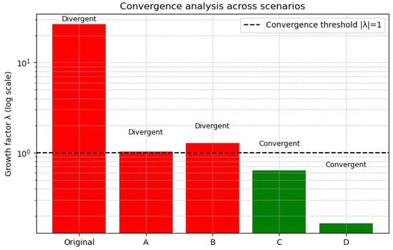
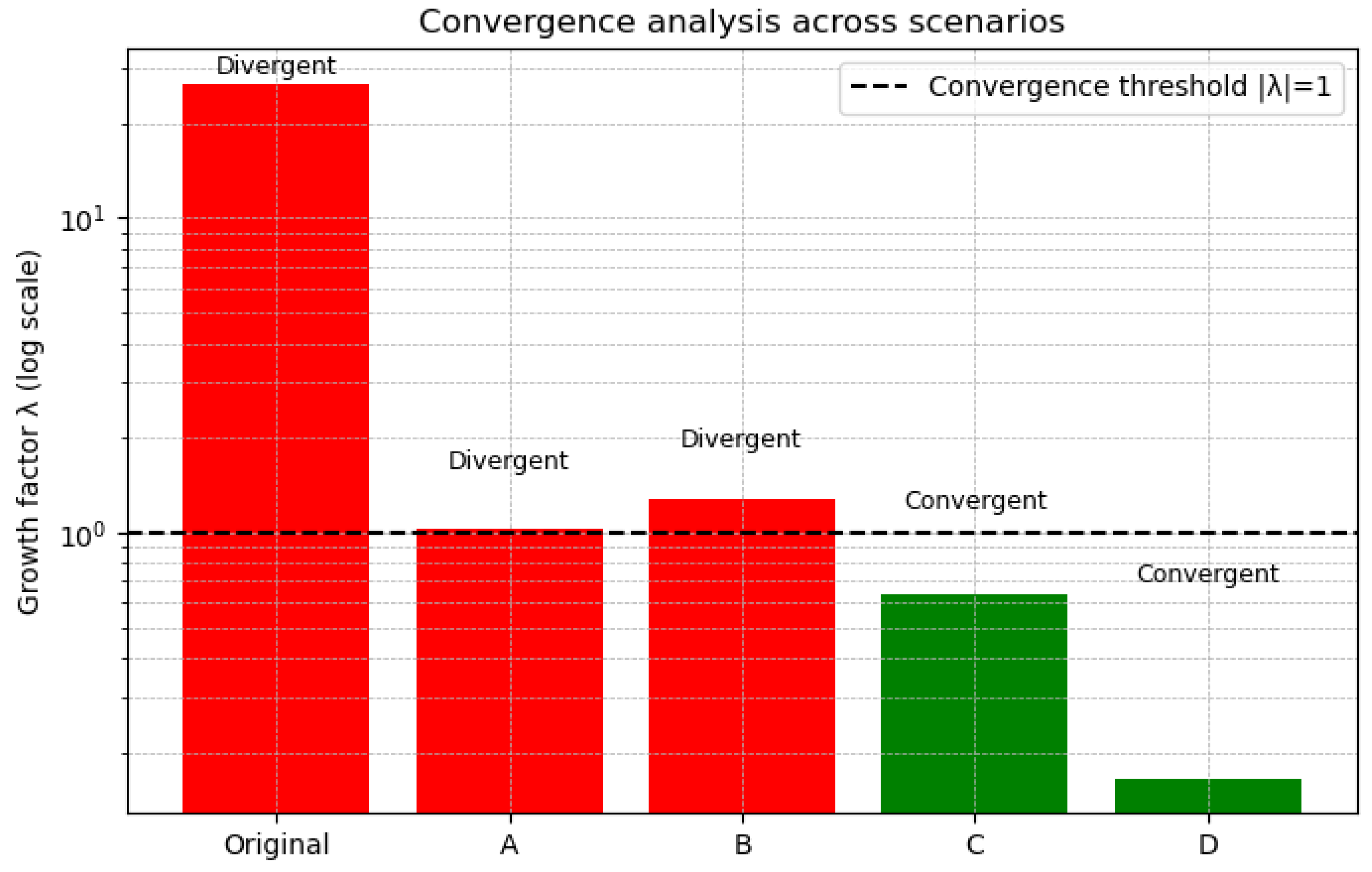
Figure 1 and Table 3 display the growth factor $\lambda$ across the different parameter scenarios (original, A, B, C, D). The vertical axis is shown in logarithmic scale to highlight the large differences between divergent and convergent cases. The dashed horizontal line at $\left|\lambda \right|=1$ marks the threshold between stability and instability. The bars in red correspond to divergent regimes ($\left|\lambda \right|>1$), where the iterative scheme explodes, and the marginal density update becomes unstable. The bars in green correspond to convergent regimes ($\left|\lambda \right|<1$), where the iteration contracts, and the density update decays toward zero. The annotations above each bar indicate the verdict (convergent or divergent) consistent with the numerical table.

Figure 1. Growth factor $\lambda$ across scenarios. Red bars indicate divergence, and green bars indicate convergence.

Table 3. Growth factor $\lambda$ and convergence verdict under different parameter scenarios.

Scenario	Parameters $(\mathit{r},\mathit{b},{\mathit{\sigma }}_{\mathit{D}})$	$\mathit{\lambda }$	Verdict
Original	$(0.020,0.50,0.24)$	$26.858$	Divergent
A	$(0.50,0.50,0.24)$	$1.0214$	Divergent
B	$(0.10,0.30,0.20)$	$1.2802$	Divergent
C	$(0.05,0.20,0.15)$	$0.633191$	Convergent (→0)
D	$(0.02,0.10,0.10)$	$0.1658$	Convergent (→0)

This graphical representation makes the convergence condition visually clear: only scenarios C and D lie below the stability threshold, while the original calibration and scenarios A and B are unstable. Financially, the figure emphasizes that excessive local volatility or too small r leads to explosive dynamics, whereas moderate volatility and weaker coupling b ensure the stability of the density iteration.

5.3. Comparative Analysis with Alternative Methods

Here, we provide a comparative discussion between our iterative scheme and three widely used approaches in computational finance: Monte Carlo simulation, deep learning models, and spectral methods. The goal is to highlight the consistency of our stability criterion based on the growth factor $\lambda$ with the qualitative behavior observed in these alternative frameworks.

5.3.1. Monte Carlo Simulation

Monte Carlo methods are flexible and widely applied in option pricing and risk management. However, they suffer from high variance and computational cost. In regimes where $\left|\lambda \right|>1$, our scheme predicts instability, and Monte Carlo simulations likewise exhibit exploding variance [34,35]. Conversely, in stable regimes ($\left|\lambda \right|<1$), Monte Carlo paths converge to well-behaved densities.

5.3.2. Deep Learning Approximation

Neural networks (ANNs, RNNs, LSTMs) have been shown to outperform classical PDE-based models in capturing nonlinear dependencies. However, their outputs also become unstable in divergent regimes, consistent with our $\lambda$ criterion [36]. In convergent regimes, deep learning models reliably approximate the density update.

5.3.3. Spectral Methods

Spectral discretizations (Chebyshev, Fourier) provide high accuracy for smooth solutions. Nevertheless, in divergent regimes, they suffer from Gibbs-type oscillations, confirming that instability is intrinsic to parameter choices rather than numerical schemes [37,38]. In convergent regimes, spectral methods yield highly accurate approximations.

Across all three alternative approaches, the stability verdict is consistent with our $\lambda$-based criterion. This demonstrates that our iterative scheme provides a transparent diagnostic tool, while Monte Carlo, deep learning, and spectral methods corroborate the same qualitative behavior. A summary of these comparisons is reported in Table 4.

Table 4. Comparison of the stability verdicts across different numerical methods.

Scenario	Monte Carlo	Deep Learning	Spectral Method
Original	Divergent (high variance)	Divergent (exploding outputs)	Divergent (oscillations)
A	Divergent	Divergent	Divergent
B	Divergent	Divergent	Divergent
C	Convergent (stable decay)	Convergent (well-learned regime)	Convergent (accurate approximation)
D	Convergent (stable decay)	Convergent (well-learned regime)	Convergent (accurate approximation)

6. Conclusions

This study demonstrated the effectiveness of the generalized Newton method in addressing the nonlinear Kolmogorov forward equation within the local stochastic volatility (LSV) model. Employing the geometric series theorem, we derived sufficient analytical conditions for convergence in the general n-dimensional setting, providing a rigorous theoretical foundation.

Building on this framework, the numerical analysis used 15 years of monthly crude oil price data (2011–2025), with the model parameters estimated statistically via maximum likelihood estimation (MLE). Convergence analysis was carried out using sensitivity tests with respect to parameter variations and initial conditions, and the results are reported in Table 3 and Figure 1. These experiments confirm that the iterative Newton scheme achieves stable convergence under realistic scenarios, while also identifying parameter ranges that lead to divergence.

From a financial perspective, the convergence of the estimated density function provides a robust approximation of the risk-neutral distribution of crude oil prices. This has direct implications for option pricing, volatility forecasting, and risk management. The results highlight that the LSV model, when combined with the generalized Newton method and supported by empirical parameter estimation, offers a tractable and accurate framework for capturing market dynamics. Compared with standard numerical schemes, the generalized Newton method demonstrates faster convergence, improved numerical stability, and reduced sensitivity to initial conditions, underscoring its practical advantages.

7. Discussion

This work has shown that the generalized Newton method offers a tractable way to analyze the nonlinear Kolmogorov forward equation within the local stochastic volatility (LSV) framework. By estimating parameters via maximum likelihood and applying the scheme to long-term crude oil data, we obtained stable convergence results supporting both the theoretical and numerical validity. The sensitivity analysis clarified how changes in the parameter and initial condition affect convergence and divergence, strengthening the model’s robustness.

Although our numerical experiments and convergence analysis were carried out in a two-dimensional setting, they provide a benchmark for stability and accuracy. For the general n-dimensional case, the applicability is theoretically supported: convergence of the iterative scheme follows from a geometric series argument applied to the Kolmogorov PDE operator, ensuring stability in higher dimensions. Thus, the two-dimensional experiments serve as practical validation, while the n-dimensional extension is analytically justified.

Nevertheless, the study is subject to simplifying assumptions and specific functional choices, which limit the full representation of market dynamics. In Table 1, we report the crude oil prices and log-returns, from which parameters were estimated via maximum likelihood using Euler–Maruyama discretization. While the dataset was expanded to improve the robustness, additional stochastic factors such as lease rates and convenience yields were not incorporated and remain natural extensions for future research.

Further work should extend the framework to multi-factor volatility models, incorporate richer datasets, and employ advanced statistical or machine learning techniques for parameter estimation and density approximation. Moreover, investigation into high-dimensional implementations, efficient parallel algorithms, and hybrid approaches combining spectral and learning-based methods would provide valuable insights. These directions will enhance the realism, robustness, and practical applicability of the methodology in financial markets and open new avenues for research on nonlinear PDEs in quantitative finance.

References

- Heston, S.L. A closed-form solution for options with stochastic volatility with applications to bond and currency options. Rev. Financ. Stud. 1993, 6, 327–343. [Google Scholar] [CrossRef] [Scilit]
- Bakshi, G.; Cao, C.; Chen, Z. Empirical performance of alternative option pricing models. J. Financ. 1997, 52, 2003–2049. [Google Scholar] [CrossRef]
- Duriš, K.; Tan, S.H.; Lai, C.H.; Sevcovic, D. Comparison of the analytical approximation formula and Newton’s method for solving a class of nonlinear Black–Scholes parabolic equations. Comput. Methods Appl. Math. 2016, 16, 35–50. [Google Scholar] [CrossRef] [Scilit]
- Company, R.; Jódar, L.; Pintos, J.R. A consistent stable numerical scheme for a nonlinear option pricing model in illiquid markets. Math. Comput. Simul. 2012, 82, 1972–1985. [Google Scholar] [CrossRef] [Scilit]
- Mashayekhi, S. Alternating direction explicit method for a nonlinear model in finance. Adv. Math. Financ. Appl. 2021, 5, 745. [Google Scholar]
- Heider, P. Numerical methods for non-linear Black–Scholes equations. Appl. Math. Financ. 2010, 17, 59–81. [Google Scholar] [CrossRef] [Scilit]
- Cui, Z.; Kirkby, J.L.; Nguyen, D. A general valuation framework for SABR and stochastic local volatility models. SIAM J. Financ. Math. 2018, 9, 520–563. [Google Scholar] [CrossRef] [Scilit]
- Saporito, Y.F.; Yang, X.; Zubelli, J.P. The calibration of stochastic local-volatility models: An inverse problem perspective. Comput. Math. Appl. 2019, 77, 3054–3067. [Google Scholar] [CrossRef] [Scilit]
- Guerrero, J.; Orlando, G. Stochastic local volatility models and the Wei–Norman factorization method. Discret. Contin. Dyn. Syst. Ser. S 2022, 15, 3699–3722. [Google Scholar] [CrossRef] [Scilit]
- Fouque, J.-P.; Papanicolaou, G.; Sircar, K.R. Derivatives in Financial Markets with Stochastic Volatility; Cambridge University Press: Cambridge, UK, 2000. [Google Scholar]
- Cont, R.; Tankov, P. Financial Modelling with Jump Processes; Chapman and Hall/CRC: Boca Raton, FL, USA, 2003. [Google Scholar]
- Saheya, B.; Chen, G.Q.; Sui, Y.K.; Wu, C.Y. A new Newton-like method for solving nonlinear equations. SpringerPlus 2016, 5, 1269. [Google Scholar] [CrossRef] [Scilit]
- Antoni, G. An efficient and straightforward numerical technique coupled to classical Newton’s method for enhancing the accuracy of approximate solutions associated with scalar nonlinear equations. Int. J. Eng. Math. 2016, 2016, 8565821. [Google Scholar] [CrossRef] [Scilit]
- Shehzad, H.T.; Anwar, M.A.; Razzaq, M. A comparative study predicting stock prices using Heston and geometric Brownian motion models. arXiv 2023, arXiv:2302.07796. [Google Scholar]
- Arregui, I.; Salvador, B.; Ševčovič, D.; Vázquez, C. Total value adjustment for European options with two stochastic factors: Mathematical model, analysis and numerical simulation. Comput. Math. Appl. 2018, 76, 725–740. [Google Scholar] [CrossRef] [Scilit]
- Wallin, M.; Ivarsson, N.; Amir, O.; Tortorelli, D. Consistent boundary conditions for PDE filter regularization in topology optimization. Struct. Multidiscip. Optim. 2020, 62, 1299–1311. [Google Scholar] [CrossRef] [Scilit]
- Boussange, V.; Becker, S.; Jentzen, A.; Kuckuck, B.; Pellissier, L. Deep learning approximations for non-local nonlinear PDEs with Neumann boundary conditions. Partial. Differ. Equ. Appl. 2023, 4, 51. [Google Scholar] [CrossRef] [Scilit]
- Glau, K.; Wunderlich, L. The deep parametric PDE method and applications to option pricing. Appl. Math. Comput. 2022, 432, 127355. [Google Scholar] [CrossRef] [Scilit]
- Mesgarani, H.; Bakhshandeh, M.; Aghdam, Y.E.; Gómez-Aguilar, J.F. The convergence analysis of the numerical calculation to price the time-fractional Black–Scholes model. Comput. Econ. 2023, 62, 1845–1856. [Google Scholar] [CrossRef] [Scilit]
- Abergel, F.; Tachet, R. A nonlinear partial integro-differential equation from mathematical finance. Appl. Math. Comput. 2010, 27, 907–917. [Google Scholar] [CrossRef] [Scilit]
- Dupire, B. Pricing and hedging with smiles. Math. Deriv. Secur. 1997, 1, 103–111. [Google Scholar]
- Atkinson, K.E.; Han, W. Theoretical Numerical Analysis: A Functional Analysis; Springer: New York, NY, USA, 2005. [Google Scholar]
- Ahmadian, D.; Rouz, O.F.; Ivaz, K.; Safdari-Vaighani, A. Robust numerical algorithm to the European option with illiquid markets. Appl. Math. Comput. 2020, 366, 124693. [Google Scholar] [CrossRef] [Scilit]
- Linz, P. Theoretical Numerical Analysis; Courier Dover Publications: New York, NY, USA, 2019. [Google Scholar]
- Kloeden, P.E.; Platen, E. Numerical Solution of Stochastic Differential Equations; Springer: Berlin, Germany, 1992. [Google Scholar]
- Fan, J.; Gijbels, I. Local Polynomial Modelling and Its Applications; Chapman & Hall: London, UK, 1996. [Google Scholar]
- Anderson, T.W. An Introduction to Multivariate Statistical Analysis, 3rd ed.; Wiley: New York, NY, USA, 2003. [Google Scholar]
- Dempster, A.P.; Laird, N.M.; Rubin, D.B. Maximum Likelihood from Incomplete Data via the EM Algorithm. J. R. Stat. Soc. Ser. B 1977, 39, 1–38. [Google Scholar] [CrossRef] [Scilit]
- Doucet, A.; de Freitas, N.; Gordon, N. Sequential Monte Carlo Methods in Practice; Springer: New York, NY, USA, 2001. [Google Scholar]
- Campbell, J.Y.; Lo, A.W.; MacKinlay, A.C. The Econometrics of Financial Markets; Princeton University Press: Princeton, NJ, USA, 1997. [Google Scholar]
- Dupire, B. Pricing with a Smile. Risk 1994, 7, 18–20. [Google Scholar]
- Gatheral, J. The Volatility Surface: A Practitioner’s Guide; Wiley: Hoboken, NJ, USA, 2006. [Google Scholar]
- Risken, H. The Fokker–Planck Equation: Methods of Solution and Applications, 2nd ed.; Springer: Berlin, Germany, 1989. [Google Scholar]
- Daniluk, A.; Lakshtanov, E.; Muchorski, R. Denoised Monte Carlo for option pricing and Greeks estimation. arXiv 2024, arXiv:2402.12528. [Google Scholar] [CrossRef] [Scilit]
- Case, G. Comparative Study of Monte Carlo and Quasi-Monte Carlo Techniques for Enhanced Derivative Pricing. arXiv 2025, arXiv:2502.17731. [Google Scholar] [CrossRef] [Scilit]
- Ding, L.; Lu, E.; Cheung, K. Deep Learning Option Pricing with Market Implied Volatility Surfaces. arXiv 2025, arXiv:2509.05911. [Google Scholar] [CrossRef] [Scilit]
- Wang, Y.; Guo, X.; Wang, K. Rational Spectral Collocation Method for Solving Black-Scholes and Heston Equations. Comput. Econ. 2024, 65, 2595–2624. [Google Scholar] [CrossRef] [Scilit]
- Rao, X.; Sawangtong, P.; Mehrdoust, F.; Najafi, A. A hybrid θ-finite difference and spectral method for multi-dimensional option pricing. J. Comput. Appl. Math. 2026, 478, 117237. [Google Scholar] [CrossRef] [Scilit]
Disclaimer/Publisher’s Note: The statements, opinions and data contained in all publications are solely those of the individual author(s) and contributor(s) and not of MDPI and/or the editor(s). MDPI and/or the editor(s) disclaim responsibility for any injury to people or property resulting from any ideas, methods, instructions or products referred to in the content. |
© 2026 by the authors. Licensee MDPI, Basel, Switzerland. This article is an open access article distributed under the terms and conditions of the Creative Commons Attribution (CC BY) license.