


Abstract
Meta-analysis of proportions requires a rigorous transformation model due to the inherent mathematical constraints of proportional data (boundedness and non-constant variance). This study compared four proportions (Untransformed, Freeman–Tukey, Logit, and Arcsine) to determine the most reliable and numerically stable estimator for pooled prevalence. A rigorous comparative evaluation was performed using 35 empirical studies on Computer Vision Syndrome (CVS)-related musculoskeletal pain prevalence. The analysis employed frequentist methods, Monte Carlo simulations (10,000 iterations) to test CI coverage, and Bayesian sensitivity analysis. Key findings were validated using the Generalized Linear Mixed Model (GLMM), representing the one-step methodological standard. Pooled prevalence estimates were highly consistent (0.467 to 0.483). Extreme heterogeneity (I2 ≈ 98–99%) persisted across all models, with τ2 values exceeding 1.0 specifically in Logit and GLMM frameworks. Mixed-effects meta-regression confirmed that this heterogeneity was independent of study size (p = 0.692 to 0.755), with the moderator explaining virtually none of the variance () of 0% to 0.2%. This confirms that the high variance is an inherent feature of the dataset rather than a statistical artifact. Simulations revealed a critical trade-off: while the Untransformed model provided minimal bias, its CI coverage failed significantly in small-sample boundary scenarios (N = 50, p = 0.01, coverage: 39.36%). Under these conditions, the PFT transformation was most robust (98.51% coverage), while the Logit model also maintained high coverage accuracy (91.07%) despite its variance inflation. We conclude that model selection should be context-dependent: the Untransformed model is recommended for well-powered datasets, whereas the PFT transformation is essential for small samples to ensure valid inferential precision.
Keywords:
meta-analysis of proportions; transformation models; generalized linear mixed model; computer vision syndrome MSC:
62P10
1. Introduction
The widespread use of digital devices has led to a significant increase in the prevalence of CVS, a multifactorial condition characterized by visual strain, headaches, and musculoskeletal pain affecting the neck, shoulders, and back [1,2]. Prolonged screen exposure induces sustained static postures, repetitive micro-movements, and ocular fatigue, which together contribute to musculoskeletal overload and chronic discomfort [3,4]. Numerous observational studies have reported varying proportions of individuals experiencing neck, shoulder, or back pain related to CVS, reflecting both occupational and ergonomic differences across populations [5,6,7,8,9].
From a quantitative perspective, meta-analysis of proportions is a key method for synthesizing such epidemiological data. However, the mathematical characteristics of proportions, bounded between 0 and 1 and exhibiting non-constant variance, make direct application of standard meta-analytic models problematic [10,11,12]. In particular, untransformed proportions tend to produce biased estimates and asymmetric confidence intervals, especially when proportions are close to 0 or 1, or when sample sizes vary widely across studies. To overcome these challenges, several variance-stabilizing transformations have been developed, each with distinct mathematical properties and inferential consequences [13,14,15,16]. Among the most widely used transformations are the logit, arcsine, and Freeman–Tukey double-arcsine (PFT) [17]. Each aims to linearize the relationship between the observed event proportion and its variance, allowing the use of inverse-variance weighting within a mixed-effects framework. The choice of transformation directly affects the pooled estimate, heterogeneity measures (τ2, I2), and the width of confidence intervals. Although these models have been extensively studied theoretically, their behavior when applied to real-world epidemiological datasets, such as those examining musculoskeletal pain in CVS, has not been systematically compared. Recent methodological reviews have shown that the PFT transformation has become one of the most widely adopted approaches for meta-analysis of proportions, with its use rising sharply over the past two decades [18]. However, despite its popularity, the justification for transformation choice is often omitted or insufficiently explained in published meta-analyses [19]. While arcsine-based transformations stabilize variance and ensure that confidence limits remain within the 0–1 range, they can also distort interpretability and introduce bias when back-transformed to the proportion scale [18,19].
Theoretical and applied work in other statistical domains reinforces these issues. For instance, Feder et al. [20] demonstrated that in the analysis of binary and proportional data, particularly in developmental and reproductive toxicology, traditional parametric models such as ANOVA can yield misleading results due to violations of normality and independence assumptions. As proportions derived from binary data often exhibit an over-dispersion or intra-cluster dependence (e.g., the “litter effect”), transformations such as the arcsine square root have been historically applied to stabilize variance [21]. However, even after transformation, mixed-effects models and logistic regression have been recommended as superior alternatives for addressing within-group correlation and non-normality [20,22]. Feder et al. [20] further emphasized the utility of simulation-based power analysis to compare transformation efficiency and model robustness under different conditions of variance and sample size, an approach conceptually analogous to Monte Carlo simulation frameworks used in modern meta-analytic evaluation.
These findings support the growing consensus that pooling methods in proportion meta-analysis should be empirically validated using both real-world and simulated data, rather than adopted purely by convention. The primary objective of this study is not to introduce new statistical theory, but to provide a rigorous mathematical comparison of the performance and inferential behavior of four pooling models and a GLMM framework in the meta-analysis of proportions related to musculoskeletal symptoms in CVS. Using data from studies on neck, shoulder, and back pain in patients with CVS, we apply and contrast four analytic approaches: Untransformed Proportions, Logit, Arcsine, and PFT. The study employs a unified analytic framework based on the restricted maximum-likelihood (REML) estimator and the Q-profile method for estimating and constructing confidence intervals for between-study variance (τ2). By analyzing how different model functions influence pooled estimates, heterogeneity, and precision, this work bridges the gap between mathematical modelling and applied health data synthesis, offering both methodological insight and practical guidance for future meta-analytic research in biomedical contexts.
2. Materials and Methods
2.1. Study Design and Objective
This study was designed as a comparative meta-analytic evaluation of mathematical models applied to proportional data, combined with Monte Carlo simulation experiments to assess the robustness of transformation methods. The dataset comprised published studies reporting the prevalence of neck, shoulder, or back pain among patients with CVS. The principal objective was to compare the performance of four modelling approaches, untransformed, arcsine, PFT, and logit transformations, in estimating pooled proportions and assessing between-study heterogeneity.
2.2. Data Sources and Inclusion Criteria
Mathematical models were constructed using data extracted from available studies conducted in populations affected by CVS. Eligible studies specifically investigated musculoskeletal complaints among participants, with a primary focus on pain localized in the neck, shoulders, and back. These outcomes were selected to reflect the most commonly reported physical symptoms associated with prolonged screen exposure and sedentary work environments. For each study, the number of cases and the total participants were extracted, allowing calculation of the observed proportion . This study did not follow a PRISMA-style systematic search strategy, as the objective was methodological comparison rather than epidemiological evidence synthesis. However, to establish a realistic empirical benchmark for testing the performance of different pooling methods, a targeted search was conducted across three databases: PubMed, Scopus, and Web of Science. The search was limited to studies published in English, covering the period from the inception of the databases until August 2025. The search string was constructed using Boolean operators (AND, OR) to combine terms related to Computer Vision Syndrome and musculoskeletal outcomes: “Computer Vision Syndrome” OR “CVS” AND “Musculoskeletal Pain” OR “Neck Pain” OR “Shoulder Pain” OR “Back Pain” OR “Prevalence”. Inclusion Criteria: Study Design: Cross-sectional or cohort studies reporting the prevalence of musculoskeletal symptoms specifically among individuals diagnosed with or exhibiting symptoms of CVS. Population: Adult digital device users (e.g., office workers, students) across various professional settings. Outcomes: Quantitative data on the prevalence of at least one musculoskeletal region (neck, shoulders, or back) associated with CVS. Measurement: Use of validated tools for CVS. Exclusion Criteria: Irrelevant Outcomes: Studies focusing solely on ocular symptoms without reporting musculoskeletal data. Specific Pathologies: Participants with pre-existing chronic spinal deformities, major trauma, or inflammatory systemic diseases (e.g., rheumatoid arthritis) that would confound prevalence estimates. Article Type: Case reports, editorials, conference abstracts, and qualitative studies.
2.3. Statistical Software
All analyses were performed using R software (version 4.3.2) with the packages meta (v6.5-0) and metafor (v4.6-0).
The command functions metaprop () and rma () were used for estimation, and the “inverse variance” method was applied in all models. Model implementation was kept identical across transformations to ensure strict comparability. Between-study variance was estimated using the Restricted Maximum Likelihood (REML) method, and confidence intervals were derived via the Q-profile method. Forest plots were generated separately for each transformation model.
2.4. Mathematical Formulation of Models
These four models were selected because they represent the most commonly used and theoretically distinct approaches for handling bounded proportions. Let denote the number of events , the sample size, and The observed proportion for the study . The selection of the four models evaluated in this study, Untransformed, PFT, Logit, and Arcsine, was strategically guided by their widespread adoption in current epidemiological and clinical literature. These models represent the primary statistical framework for the majority of published meta-analyses of proportions, as evidenced by large-scale empirical reviews [23].
Except for the untransformed approach, the following transformations were applied to stabilize variance and achieve approximate normality of sampling distributions. To address numerical instability associated with boundary values (proportions of 0 or 1), a continuity correction was implemented in accordance with standard meta-analytic practices. For the Logit, Arcsine, and Untransformed models, a constant of 0.5 was algorithmically added to all cells (Haldane–Anscombe correction) when studies with zero events were encountered during the simulation iterations to ensure the calculation of variance and standard errors. Conversely, the PFT was specifically utilized for its ability to handle boundary values through its unique mathematical structure.
which accommodates 0 and 1 values without the need for external continuity corrections, thus preserving the original weighting of the studies. PFT estimates were back-transformed using the harmonic mean of sample sizes (). Unlike the arithmetic mean, the harmonic mean is less sensitive to sample size outliers and effectively stabilizes variance across diverse populations. This approach is the established standard for minimizing bias when restoring proportions from the double-arcsine scale.
- Untransformed Proportion
This direct approach assumes approximate normality of proportions and serves as a baseline for comparison.
- 2.
- Arcsine Transformation
Back-transformation to the original scale was obtained using the following:
- 3.
- Freeman–Tukey Double Arcsine Transformation
Back-transformation to the proportion scale [14] used the harmonic mean of sample sizes :
where, the harmonic mean is calculated as follows:
- 4.
- Logit Transformation
2.5. Generalized Linear Mixed Model (GLMM)
In addition to the four classical proportion-based models (Untransformed, PFT, Logit, and Arcsine), a GLMM framework was also applied as a supplementary analytical approach. Although not the primary objective of this study, the inclusion of GLMM aimed to evaluate whether the conventional transformation-based random-effects models yield comparable pooled estimates and heterogeneity measures to those obtained under a likelihood-based approach. GLMMs offer a unified modelling structure for binomial outcomes without the need for variance-stabilizing transformations. Each study’s event count is assumed to follow a binomial distribution:
where is the overall mean on the logit scale, and represents between-study variance. This formulation is mathematically equivalent to a random-intercept logistic regression, estimated via maximum likelihood. The GLMM model was implemented in R using the metafor and meta packages (functions rma.glmm () and metaprop (method = “GLMM”)), employing adaptive Gaussian quadrature for numerical integration. While the main objective of this study was to mathematically compare transformation-based models, GLMM results were included for comparative validation, assessing whether transformation-free likelihood estimation leads to systematic deviation or improved precision relative to traditional methods. This extension addresses recent recommendations from methodological literature suggesting that GLMMs provide more accurate estimation for extreme proportions and small-sample studies by directly modelling the binomial variance structure rather than relying on approximate normality. The GLMM approach was included solely for comparative validation and was not considered a primary analytic method, in accordance with the study’s methodological scope.
2.6. Meta-Analytic Model
Each proportion was analyzed using both fixed-effect and random-effects models.
In the fixed-effect model, it is assumed that all studies estimate the same underlying true effect (θ) and that the only source of variation across studies arises from within-study sampling error. The between-study variance (τ2) is therefore assumed to be zero.
Let, for each study :
= proportion (e.g., Logit, Arcsine, PFT, or Untransformed proportion)
= within-study variance of that transformed value.
Then, the pooled estimate under the fixed-effect model is calculated as follows:
where the weights are defined as follows:
The variance of the pooled estimate is given by the following:
The 95% confidence interval is expressed as follows:
where:
- : Pooled effect estimates under the fixed-effect model;
- Critical value from the standard normal distribution ();
- : Variance of the pooled estimate.
After the pooled estimate is obtained on the transformed scale, it is back-transformed to the proportion scale using the appropriate inverse transformation for arcsine or p = .
The random-effects model assumes that true effects vary across studies due to both within-study error and between-study heterogeneity. Thus, each study is assumed to estimate its own true effect θₖ, which follows a normal distribution with mean θ and variance τ2:
The random-effects model is expressed as follows:
with variance
and corresponding confidence interval:
However, in meta-analysis of proportions, the Clopper–Pearson CI affects only the display of individual studies in the forest plot, while the pooled CI is still computed using variances and weights (due to the fixed model).
Thus,
For each study:
where:
- = number of events;
- = total number of participants;
- = inverse cumulative distribution function of the Beta distribution.
This is an exact interval, particularly important when proportions are extreme ().
Between-study heterogeneity was quantified using the following:
where () is Cochran’s heterogeneity statistic.
2.7. Model Comparison and Interpretation
For each pooling method, pooled proportions and 95% confidence intervals were back-transformed to the original probability scale for interpretability. While the Untransformed model operates directly on the raw scale, results from the Logit, Arcsine, and PFT were mapped back to ensure comparability.
Estimates of (), (), and () statistics were compared to assess model sensitivity to heterogeneity. Differences among the estimation approaches were interpreted both mathematically (in terms of variance stabilization for transformation-based models) and practically (in terms of pooled prevalence estimates). Forest plots were visually inspected for consistency of point estimates and interval overlap across all four models.
2.8. Sensitivity and Robustness Analysis
To assess the numerical accuracy, precision, and robustness of the four transformation models for proportion meta-analysis, a comprehensive Monte Carlo simulation framework was implemented in R. Each simulation iteration generated study-level event counts from a binomial distribution with a predefined true proportion p true and sample size n. The simulation was designed to mirror the empirical structure of our research, which included results from 35 primary studies. These studies provided a total of k = 54 individual data points, as several publications reported independent prevalence rates for different anatomical regions (e.g., neck, shoulder, and back pain). Consequently, each simulation iteration generated k = 54 independent study-level estimates to ensure that the performance of the models was evaluated under conditions representative of the actual CVS dataset. The simulations were designed to represent realistic conditions of meta-analyses of proportions, including small, moderate, and large samples (n = 50, 200, 1000) and a range of true event probabilities (). Regarding the untransformed proportions model, we monitored the confidence intervals for potential boundary violations (values outside the [0, 1] range). It was pre-specified that truncation would only be applied if the normal approximation produced logically inconsistent estimates. In the simulation phase, raw values were maintained to assess the unbiased performance of each pooling method, and no out-of-bounds intervals were observed in the final analysis. For each proportion model, Untransformed, PFT, Logit, and Arcsine, the pooled prevalence estimates were computed using the inverse-variance method under a random-effects framework with REML estimation of between-study variance (). The bias and Root Mean Squared Error (RMSE) were computed across repeated simulations as measures of systematic deviation and total estimation error, respectively:
where N is the total number of iterations (set to 1000 and 10,000 in two independent simulation experiments). The Bias quantifies systematic over- or underestimation of the true proportion, while the RMSE incorporates both bias and random variability. Lower RMSE values correspond to more stable and accurate estimators across replications. Additionally, the coverage probability of the nominal 95% confidence interval (CI) was estimated for each proportion model, representing the proportion of simulations in which the true parameter p true was contained within the computed CI.
2.9. Bayesian Sensitivity Analysis
To further assess the robustness and consistency of inference across paradigms, a Bayesian random-effects meta-analysis was performed for each of the four proportion models (Untransformed, PFT, Logit, and Arcsine) using the bayesmeta package in R. The Bayesian model formulation paralleled the frequentist random-effects structure, assuming that each study-specific transformed effect follows a normal likelihood:
where μ represents the overall pooled effect, and denotes the between-study variance. An improper uniform prior was assigned to the overall mean effect μ to represent non-informative belief, and a half-normal prior was assigned to the heterogeneity parameter τ (scale = 0.5), following the recommendations of Röver et al. [24]. Posterior distributions for μ and τ were obtained via numerical integration, and maximum a posteriori (MAP) and marginal likelihood estimates were extracted for comparison with frequentist REML results. For each model, posterior summaries (mode, median, mean, 95% credible interval) were computed for both parameters, along with the posterior I2, defined as follows:
where denotes the average within-study variance on the transformed scale.
3. Results
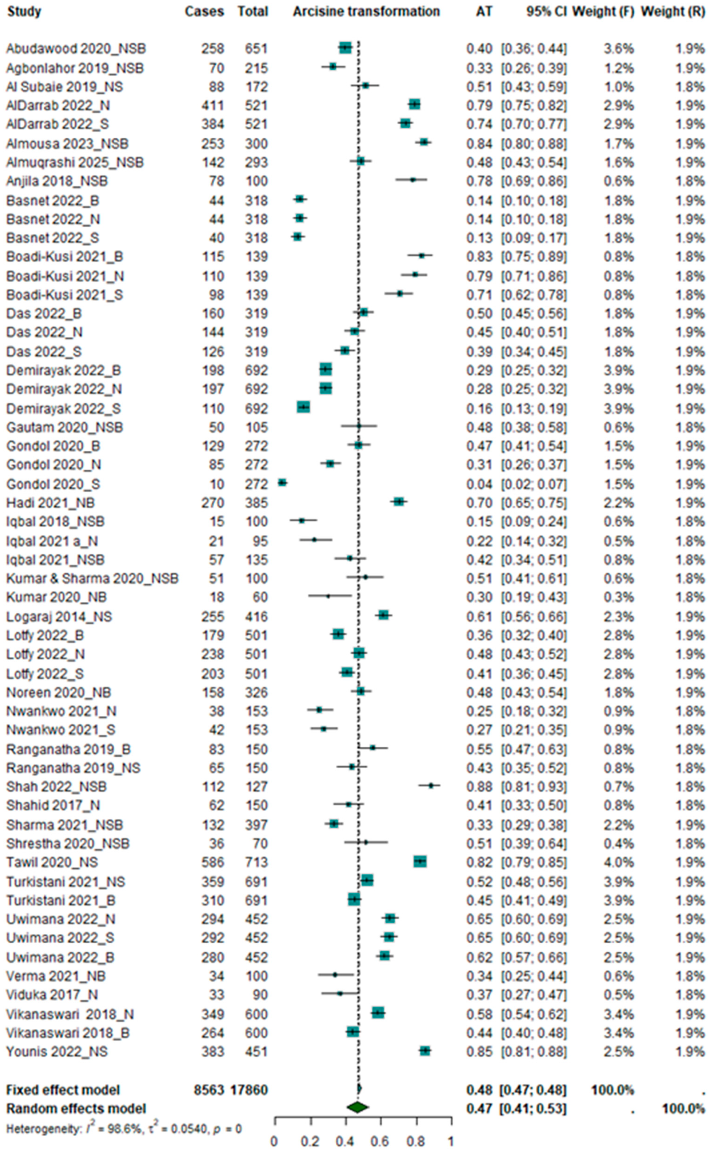
A total of 35 studies (k = 54) encompassing 10,359 participants were included in the four meta-analytic models. The pooled prevalence of musculoskeletal pain (neck, shoulder, or back pain associated with CVS was estimated using four proportion approaches: Untransformed, PFT, Logit, and Arcsine. All analyses were performed using the inverse variance method under both fixed-effect and random-effects models, applying the REML estimator for between-study variance (τ2) and Q-profile confidence intervals. Across all models, pooled prevalence estimates were highly consistent, ranging from across transformation methods (Figure 1, Figure 2, Figure 3 and Figure 4). The untransformed model showed comparable accuracy but slightly higher variance, while the logit transformation, though stable, exhibited larger τ2 due to variance inflation at boundary proportions (Table 1).
Table 1.
Empirical results.
Across all four proportion models, the moderator log (sample size) showed no statistically significant association with effect estimates (). The proportion of heterogeneity explained by sample size was in every model, indicating that study size did not account for between-study variability. Residual heterogeneity remained high () regardless of transformation, suggesting that other factors may be driving the observed variation (Table 2, Figure A1). A supplementary GLMM was also estimated to provide a likelihood-based validation of transformation-based results, following current methodological recommendations for meta-analysis of proportions [25,26]. Although not the primary aim of this study, the GLMM was included to evaluate whether a transformation-free, model-based estimation approach yields similar pooled estimates and heterogeneity measures. The GLMM results closely mirrored those from the Logit model, with nearly identical pooled prevalence under both fixed-effect (0.4830, 95% CI: 0.475–0.491) and random-effects models (0.4665, 95% CI: 0.399–0.536). The estimated between-study variance and heterogeneity were also consistent with the transformation-based approaches, confirming that GLMM estimation provides equivalent inferential outcomes when data exhibit strong between-study variability (Table 1). These findings suggest that, while transformation-based models remain numerically stable and widely interpretable, GLMM approaches can serve as an analytically robust alternative that avoids the need for variance-stabilizing transformations. Given the computational complexity and marginal differences in results, GLMM was retained as a supplementary verification method rather than a primary analytic framework in this study.
Table 2.
Mixed-effects meta-regression results with log-transformed sample size as moderator.
Figure 1.
Untransformed proportion; N—neck pain; S—shoulder pain; B—back pain; NSB—neck, shoulder, back pain; NS—neck, shoulder pain; NB—neck, back pain. Square sizes are proportional to study weights, horizontal lines indicate 95% confidence intervals, and the diamond represents the pooled estimate [27,28,29,30,31,32,33,34,35,36,37,38,39,40,41,42,43,44,45,46,47,48,49,50,51,52,53,54,55,56,57].
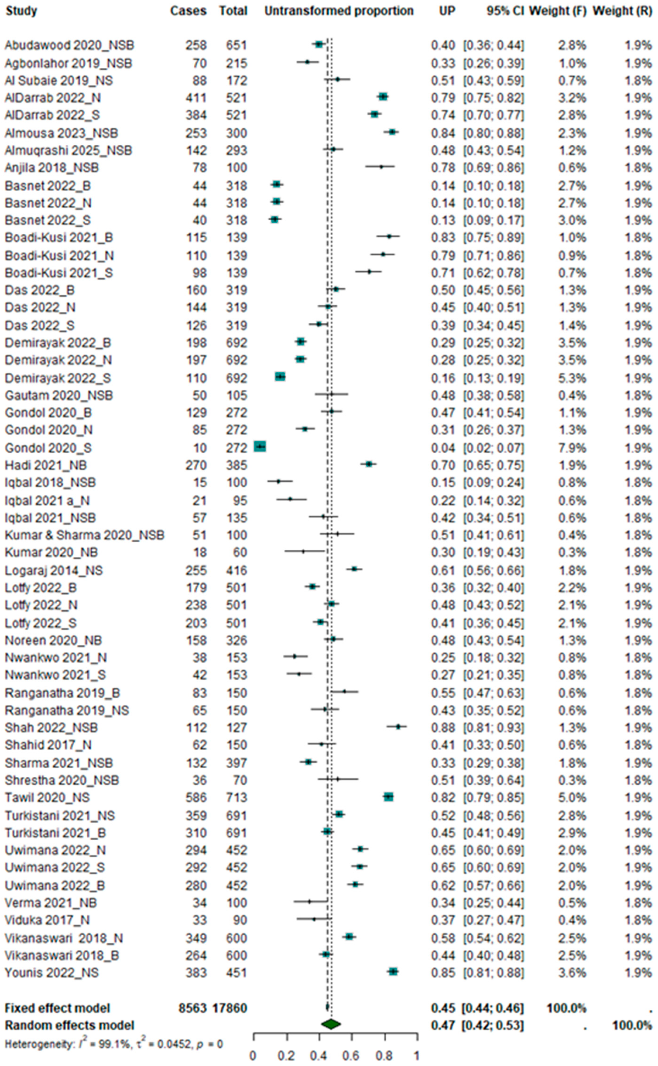
Figure 2.
Freeman–Tukey Double Arcsine Transformation; N—neck pain; S—shoulder pain; B—back pain; NSB—neck, shoulder, back pain; NS—neck, shoulder pain; NB—neck, back pain. Square sizes are proportional to study weights, horizontal lines indicate 95% confidence intervals, and the diamond represents the pooled estimate [27,28,29,30,31,32,33,34,35,36,37,38,39,40,41,42,43,44,45,46,47,48,49,50,51,52,53,54,55,56,57].
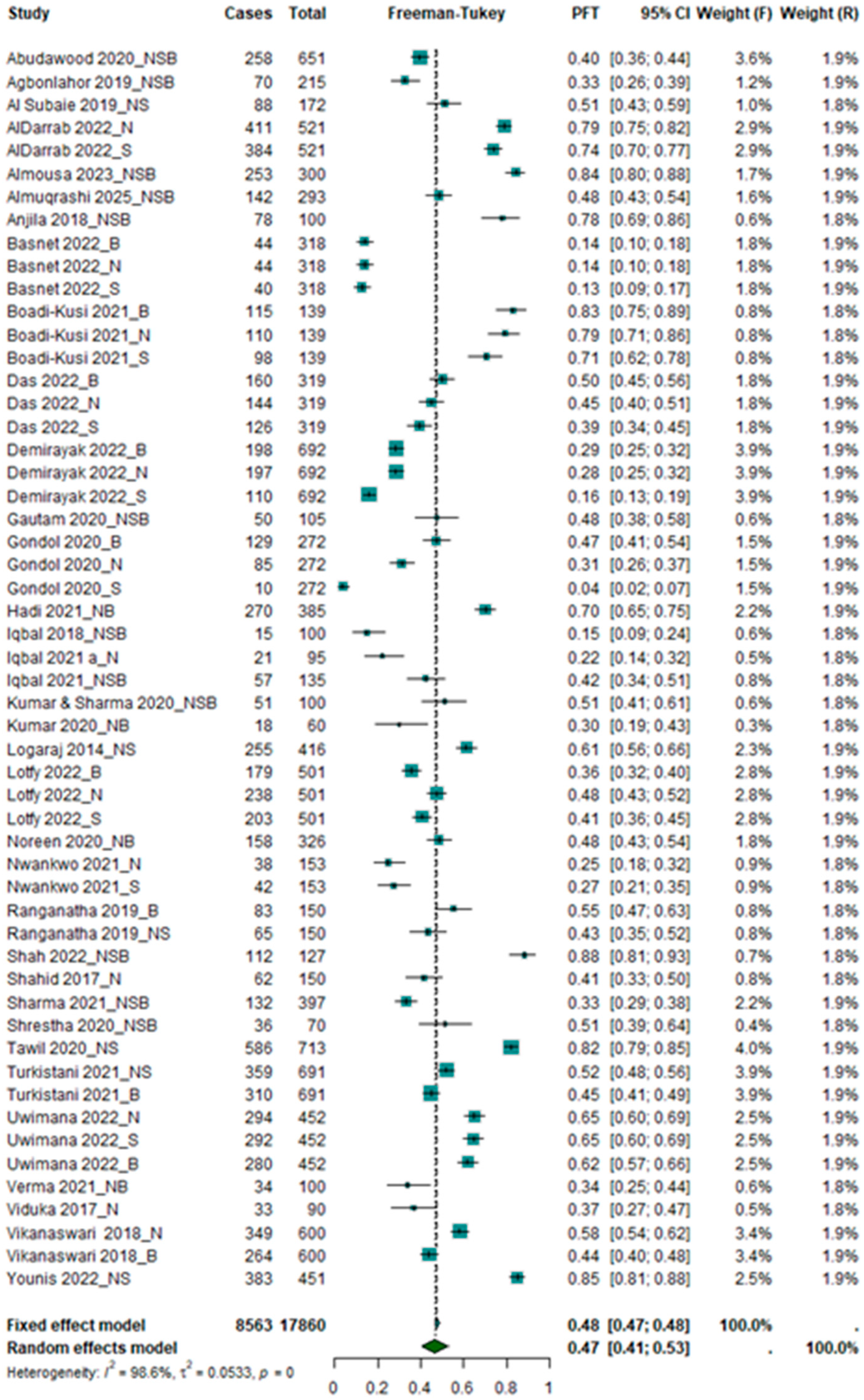
Figure 3.
Logit transformation; N—neck pain; S—shoulder pain; B—back pain; NSB—neck, shoulder, back pain; NS—neck, shoulder pain; NB—neck, back pain. Square sizes are proportional to study weights, horizontal lines indicate 95% confidence intervals, and the diamond represents the pooled estimate [27,28,29,30,31,32,33,34,35,36,37,38,39,40,41,42,43,44,45,46,47,48,49,50,51,52,53,54,55,56,57].
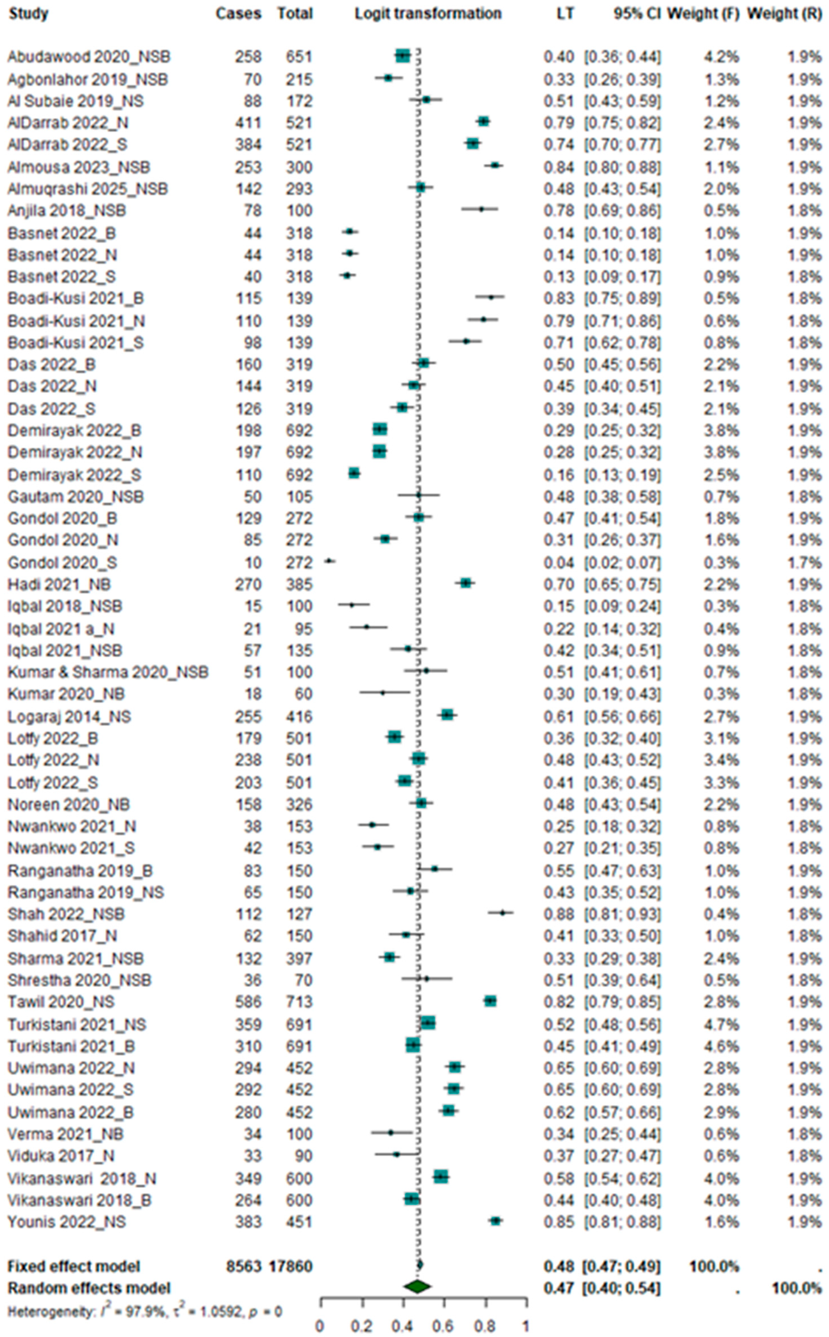
Figure 4.
Arcsine transformation; N—neck pain; S—shoulder pain; B—back pain; NSB—neck, shoulder, back pain; NS—neck, shoulder pain; NB—neck, back pain. Square sizes are proportional to study weights, horizontal lines indicate 95% confidence intervals, and the diamond represents the pooled estimate [27,28,29,30,31,32,33,34,35,36,37,38,39,40,41,42,43,44,45,46,47,48,49,50,51,52,53,54,55,56,57].
To assess model stability under sampling variability, Monte Carlo simulations with 1000 and 10,000 iterations were performed. The 1000-run simulation revealed minimal bias for the untransformed model and substantial systematic bias for the PFT and Arcsine transformations , while the logit model displayed the largest deviation . Only the untransformed model achieved complete coverage of the nominal 95% confidence interval , suggesting that its interval estimates are more conservative and robust (Table 3).
Table 3.
Comparison of bias, RMSE, and 95% CI coverage across four proportion transformations under Monte Carlo scenarios (n = 1000 iterations).
The extended 10,000-run simulation confirmed these tendencies under more extreme distributional conditions, producing a systematic upward bias of approximately 0.53 across all models, consistent with overestimation under near-boundary probabilities. Coverage analysis again showed full inclusion for the untransformed model and collapse for the other three transformations, indicating that variance-stabilizing transformations may underperform in extreme, skewed conditions (Table 4).
Table 4.
Comparison of bias, RMSE, and 95% CI coverage across four proportion transformations under Monte Carlo scenarios (n = 10,000 iterations).
To further assess the robustness of these proportions, Monte Carlo simulations with 10,000 iterations were performed across varying true proportions (0.01, 0.1, 0.5, 0.9, 0.99) and sample sizes (N = 50, 200, 1000) (Table 5, Figure A2). In small samples (N = 50), the Logit and PFT transformations achieved the most stable coverage across the range of true proportions (98.51 and 91.07% at p = 0.01). The Untransformed and Arcsine models performed poorly at extreme proportions (p < 0.1 or p > 0.9), with coverage rates dropping significantly (e.g., 39.36% and 37.89%, respectively, at p = 0.01), indicating highly unreliable confidence intervals. With a moderate sample size (N = 200), all models showed improved performance; however, PFT remained the most consistent at distribution tails (98.27% coverage), while the Untransformed model still exhibited substantial under-coverage (86.77%) at extreme proportions. In large samples (N = 1000), all models stabilized, approaching the theoretical 0.95 coverage. Arcsine and PFT achieved nearly perfect rates (95.67% and 94.29%, respectively). The simulation confirmed that variance-stabilizing transformations particularly PFT yield superior confidence interval coverage, particularly under extreme event probabilities and small sample conditions (Table 5).
Table 5.
Monte Carlo simulation results for confidence interval coverage rates (%).
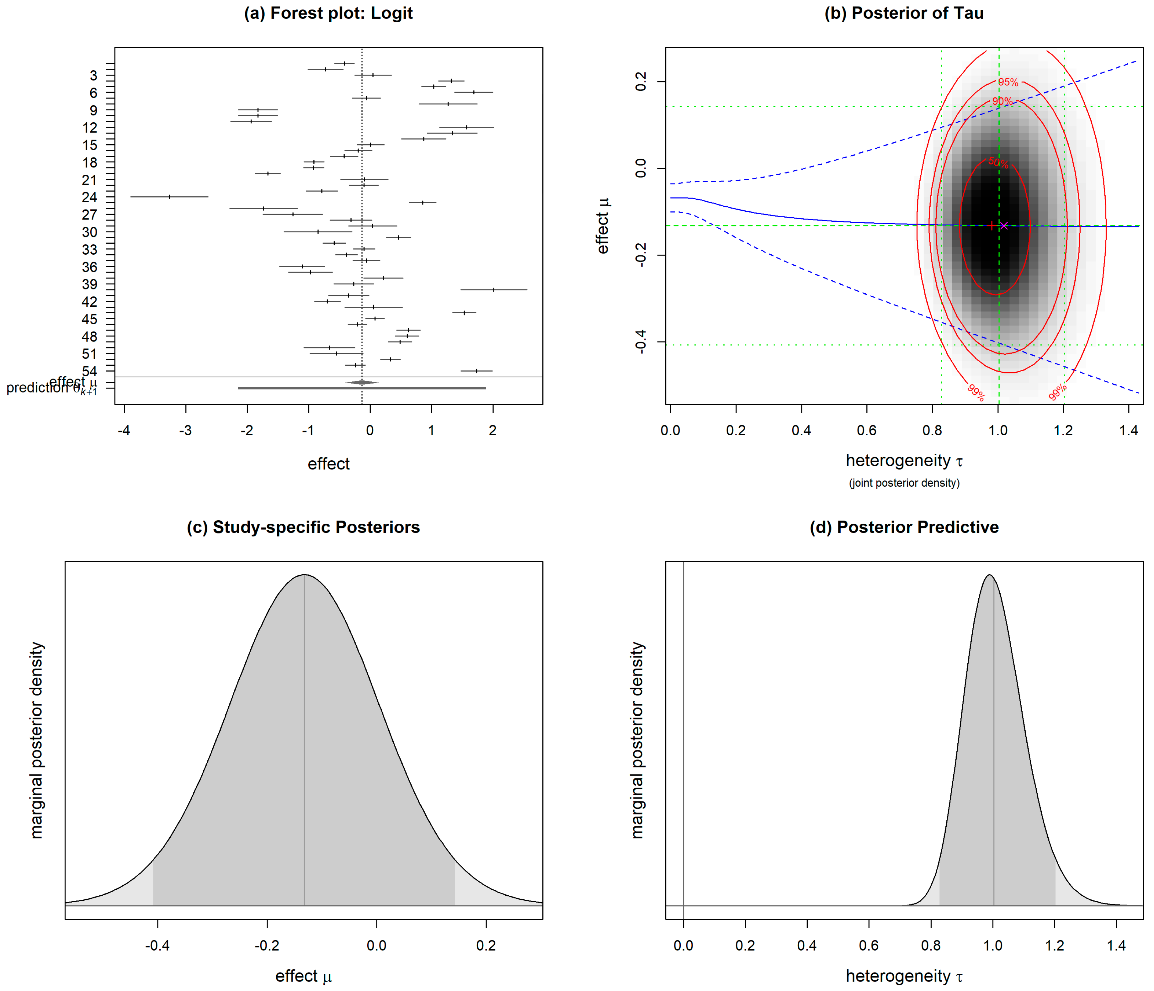
To further evaluate model robustness, a Bayesian random-effects meta-analysis was performed for each transformation using the bayesmeta package in R. The analysis applied an improper uniform prior for the overall effect (μ) and a half-normal prior for between-study heterogeneity (τ). Across all transformations, posterior summaries closely matched the frequentist REML estimates, indicating consistency of inference across paradigms. The posterior means for τ ranged between 0.21 and 0.24, except for the logit model , which exhibited greater dispersion consistent with its nonlinear scale.
The 95% credible intervals for μ overlapped substantially across the Arcsine and PFT transformations, both centered around 0.75. The relative heterogeneity (posterior I2) was uniformly high across models, confirming the presence of strong inter-study variation consistent with the empirical Q-statistics (Table 6). The near equality between MAP and REML estimates suggests that the posterior distributions were largely data-driven rather than prior-influenced. Overall, Bayesian inference corroborated the frequentist results, demonstrating that the Arcsine and PFT transformations provide stable central estimates and reasonable uncertainty quantification, whereas the Logit model overstates heterogeneity under extreme proportions (Figure A3, Figure A4, Figure A5 and Figure A6).
Table 6.
Bayesian meta-analysis.
4. Discussion
The present study evaluated four commonly used methods for pooling proportions in meta-analysis: Untransformed, PFT, Logit, and Arcsine, using both empirical and simulation-based approaches to determine the most reliable and numerically stable estimator for pooled prevalence.
4.1. Empirical Findings
Based on 35 studies (k = 54), all four pooling approaches produced remarkably consistent pooled estimates of prevalence, ranging narrowly from 0.467 to 0.483. This high concordance across methods suggests that for this specific, moderately sized dataset, the choice of transformation does not significantly alter the final central estimate of musculoskeletal pain prevalence. However, a uniform issue across all models was the persistence of extreme inter-study heterogeneity . This observed level of heterogeneity is consistent with recent empirical evidence in prevalence meta-analyses; for instance, Migliavaca et al. [23] reported a median I2 of 96.9% across 134 studies, suggesting that such high values are often a mathematical consequence of the data type and study count rather than an indicator of low credibility. This confirms that the observed variation is inherent to the dataset itself, driven by underlying differences among studies (e.g., population, case definition, setting), rather than being a consequence of model instability or transformation choice. Crucially, the meta-regression confirmed that study size did not account for this variability. The moderator showed no statistically significant association with effect estimates ( across all models), and the proportion of heterogeneity explained was in every model. This indicates that the search for heterogeneity drivers must focus on other study-level factors (e.g., methodological quality, geographical location).
4.2. Estimator Robustness and Simulation Findings
Importantly, the superior CI coverage of the Untransformed model should be interpreted separately from the numerical stability of central estimates, where the arcsine transformation performed well in midrange probability settings. Monte Carlo simulations were instrumental in evaluating estimator performance under controlled scenarios. While the empirical analysis found minimal bias exclusively for the Untransformed model in the 1000-iteration scenario (Bias = −0.0058, Table 3), the simulations revealed critical differences concerning uncertainty quantification. In the extended 10,000-iteration simulation (Table 4), although all models exhibited substantial systematic bias, the Untransformed model was unique in maintaining complete coverage (Coverage = 1.0). In contrast, PFT, Arcsine, and Logit transformations displayed zero coverage under these conditions. This suggests that the Untransformed model’s interval estimates are more robust and reliable when boundary proportions are approached, as evidenced by its superior coverage performance across both simulation settings (Table 3 and Table 4). However, these general simulation findings must be contextualized through a more granular analysis of specific sample size and probability interactions. While the Untransformed model appears superior in large-scale, aggregated simulations, data from Table 5 reveal a critical trade-off when the models are subjected to “stress tests” at the distribution edges. At N = 50 and p = 0.01, the Untransformed model’s coverage, previously near-perfect in global scenarios, drops to a failing 39.36%, and the Arcsine transformation similarly underperforms at 37.89%. However, Arcsine shows the fastest recovery rate; as soon as the sample increases to N = 1000, its coverage jumps to 95.67%, thus reaching the nominal confidence level. This suggests that Arcsine is not a one-size-fits-all tool, but a model whose reliability critically depends on the power of the data set itself. This divergence suggests that the high coverage observed in Table 3 and Table 4 reflects the models’ performance in “average” or well-powered conditions, whereas Table 5 exposes their vulnerability in small-sample boundary settings. Under these identical small-sample conditions, the PFT proves to be the most resilient, maintaining 98.51% coverage. This indicates that the PFT’s capacity for variance stabilization is specifically optimized for those cases where the binomial variance is most unstable. Nevertheless, as the sample size increases to N = 1000, the discrepancies between the models diminish. At this larger scale, even the Arcsine and Untransformed models converge toward nominal levels (95.67% and 92.71%), demonstrating that the choice of model becomes less critical for inferential validity as the dataset becomes well-powered. However, Arcsine shows the fastest recovery rate; as soon as the sample increases to N = 1000, its coverage jumps to 95.67%, thus reaching the nominal confidence level. This suggests that Arcsine is not a one-size-fits-all tool, but a model whose reliability critically depends on the power of the data set itself. The Logit model, on the other hand, represents a unique case. While Table 5 shows it maintains robust coverage in small samples (91.07%), our empirical and Bayesian analyses (Table 1 and Table 6) reveal a significant cost for this robustness: a pronounced inflation of between-study variance . This suggests that the Logit model achieves its coverage by overstating uncertainty, making it a conservative but less precise estimator in the presence of strong inter-study heterogeneity.
4.3. Bayesian Sensitivity Analysis
The Bayesian sensitivity analysis corroborated the frequentist results from a probabilistic perspective. Posterior summaries (MAP and MAP) were closely aligned with frequentist REML estimates, suggesting that the posterior inference was data-driven rather than prior-dominated. This equivalence across inferential paradigms confirms that the Arcsine and PFT transformations provide stable central estimates, while the Logit model overstates heterogeneity.
4.4. Comparison with Previous Research
Our study confirmed that while the final pooled proportion was highly consistent across methods, the Logit transformation exhibited a pronounced tendency to inflate between-study variance (). Furthermore, the Logit transformation offers an additional benefit: the regression slope has a direct, physically interpretable meaning (related to the odds ratio). Despite these advantages, the primary finding in the literature, supported by our simulation results, is the shift toward one-step methods (GLMMs, or advanced Bayesian models) for synthesising proportions [58]. The contemporary literature increasingly suggests that one-step methods are generally superior, as they avoid the numerical distortions inherent in two-step transformations and may lead to substantially different, and potentially more accurate, results [19]. Beyond the frequentist frameworks evaluated here, modern hierarchical Bayesian models and robust meta-analytic methods represent another sophisticated layer of one-step approaches. While these methods were outside the primary scope of this comparative study of commonly used pooling approaches, they offer promising tools for methodological triangulation, especially in datasets where incorporating prior information or handling extreme outliers is a priority. To validate the consistency of our final pooled estimate and the magnitude of heterogeneity, we executed the GLMM with a Logit-Binomial structure, representing the methodologically superior one-step approach. The GLMM Random-Effects model yielded a pooled proportion of 0.466 ), which was highly consistent with the pooled estimates from all four conventional two-step models, particularly the Logit model (0.4669), confirming the numerical stability of the final result (Table 1). The high consistency between the Logit-transformed model and the GLMM benchmark stems from their shared use of the logit link function. While the standard Logit model uses summarized data (two-step approach), the GLMM models the binomial likelihood directly (one-step approach), avoiding continuity corrections and handling study weights more robustly under extreme heterogeneity. This convergence confirms that the prevalence estimates are not artifacts of the transformation process itself. More critically, the GLMM confirmed an extreme residual heterogeneity (, ), virtually identical to the two-step Logit estimate . This crucial finding demonstrates that the substantial inflation of between-study variance is an inherent feature of the dataset and not a statistical artefact of the two-step Logit transformation, reinforcing the need to investigate clinical or methodological sources of heterogeneity. Furthermore, the GLMM meta-regression analysis of the sample size confirmed that this moderator was not statistically significant (), with an extremely low explained variance (), suggesting that sample size does not contribute to the observed variability. This confirms that the logit-binomial likelihood yields nearly identical results to the transformation-based approach under extreme heterogeneity. Consequently, the robustness demonstrated by the Untransformed model in our study, particularly its minimal bias and complete coverage in high-iteration scenarios (Table 3 and Table 4), validates its continued practical use in well-powered datasets. However, the Arcsine transformation’s effectiveness was partially mitigated by the extreme inter-study heterogeneity observed in our empirical data (τ2 = 0.054, Table 1). Our simulation results in Table 5 further reveal that the Arcsine model is highly sensitive to sample size; at N = 50 and p = 0.01, its coverage drops to a critical 37.89%, performing no better than the Untransformed approach. However, the necessity of the two-step transformation persists in practical application: When meta-analysts need to visualize study-specific estimates using tools like the Forest Plot or the Funnel Plot (to assess potential publication bias or small-study effects) [58,59,60], the standard two-step approach is required, as GLMMs and Bayesian models do not easily yield the necessary study-specific standard errors and confidence intervals. For such visualizations, our findings suggest a refined approach: while the Arcsine transformation is reliable for large-scale datasets where it converges toward nominal coverage (95.67% at N = 1000, Table 5), the PFT emerges as a far superior and more robust choice for smaller samples, maintaining an exceptional 98.51% coverage rate under extreme event probabilities (Table 5).
5. Practical Implications and Conclusions
The present study highlights that the choice of proportion model in meta-analysis has practical consequences for accurately quantifying the prevalence of musculoskeletal pain associated with CVS. Reliable estimation of such prevalence is essential for guiding ergonomic and occupational health interventions. Among the evaluated approaches, the Untransformed model provided the most interpretable and stable results with consistent confidence interval coverage in large-sample scenarios. However, our simulation results in Table 5 reveal that the Untransformed model and the Arcsine transformation both suffer from a dramatic loss of coverage (dropping to approximately 39% and 38%, respectively) when dealing with small sample sizes (N = 50) and extreme event probabilities (p = 0.01). In contrast, the PFT transformation emerged as the most robust alternative under these challenging conditions, maintaining a superior coverage rate of 98.51%. Similarly, the Logit model demonstrated high coverage accuracy in small samples (91.07%), though it exhibited a pronounced tendency to inflate between-study variance in our highly heterogeneous empirical dataset (τ2 = 1.056). This convergence supports the methodological equivalence between transformation-based and model-based approaches for well-powered datasets, while emphasizing that the choice of a specific estimator is paramount for smaller, more volatile samples. From a methodological standpoint, these results reinforce the importance of explicitly reporting the transformation or modelling approach used. For robust and reproducible inference, researchers are advised to prioritize the Untransformed model for well-powered, large-scale meta-analyses, but to utilize the PFT when accurate confidence interval coverage is essential for small samples or boundary event probabilities. The pooled prevalence of neck, shoulder, and back pain associated with CVS was consistently estimated across all models in a narrow range of 46.7% to 48.3%, thus establishing a robust, evidence-based benchmark for guiding occupational health and ergonomic interventions. Therefore, these findings emphasize that the rigorous selection of a mathematically stable estimator is paramount for providing the most accurate and actionable clinical prevalence estimate for this widespread musculoskeletal issue.
Author Contributions
Conceptualization, V.D. and B.O.; methodology, P.D.; software, V.D.; validation, P.D. and M.P.; formal analysis, V.D.; investigation, M.P.; resources, P.D.; data curation, B.R.; writing—original draft preparation, V.D. and M.P.; writing—review and editing, B.R.; visualization, B.O.; supervision, P.D.; project administration, B.R.; funding acquisition, B.O. All authors have read and agreed to the published version of the manuscript.
Funding
This research was supported by the Provincial Secretariat for Higher Education and Scientific Research of AP Vojvodina, grant number: 00380417 2025 09418 003 000 000 001.
Data Availability Statement
All original contributions presented in this study are included in the article. Additional information may be obtained from the corresponding authors upon reasonable request.
Conflicts of Interest
Certain authors are affiliated with non-academic institutions. The authors declare no commercial or financial relationships that could be construed as a potential conflict of interest.
Abbreviations
The following abbreviations are used in this manuscript:
| ANOVA | Analysis of Variance |
| CI | Confidence Interval |
| CP | Clopper–Pearson (confidence interval) |
| CVS | Computer Vision Syndrome |
| FE | Fixed-Effect (model) |
| GLMM | Generalized Linear Mixed Model |
| MAP | Maximum A Posteriori |
| PAS | Arcsine-transformed proportion |
| PFT | Freeman–Tukey double-arcsine transformed proportion |
| PLO | Logit-transformed proportion |
| PRAW | Untransformed (raw) proportion |
| PRISMA | Preferred Reporting Items for Systematic Reviews and Meta-Analyses |
| RE | Random-Effects (model) |
| REML | Restricted Maximum Likelihood |
| RMSE | Root Mean Squared Error |
| VDT | Visual Display Terminal |
Appendix A
Table A1.
Studies whose results are included.
Figure A1.
Regression analysis of moderation (log (Total)).
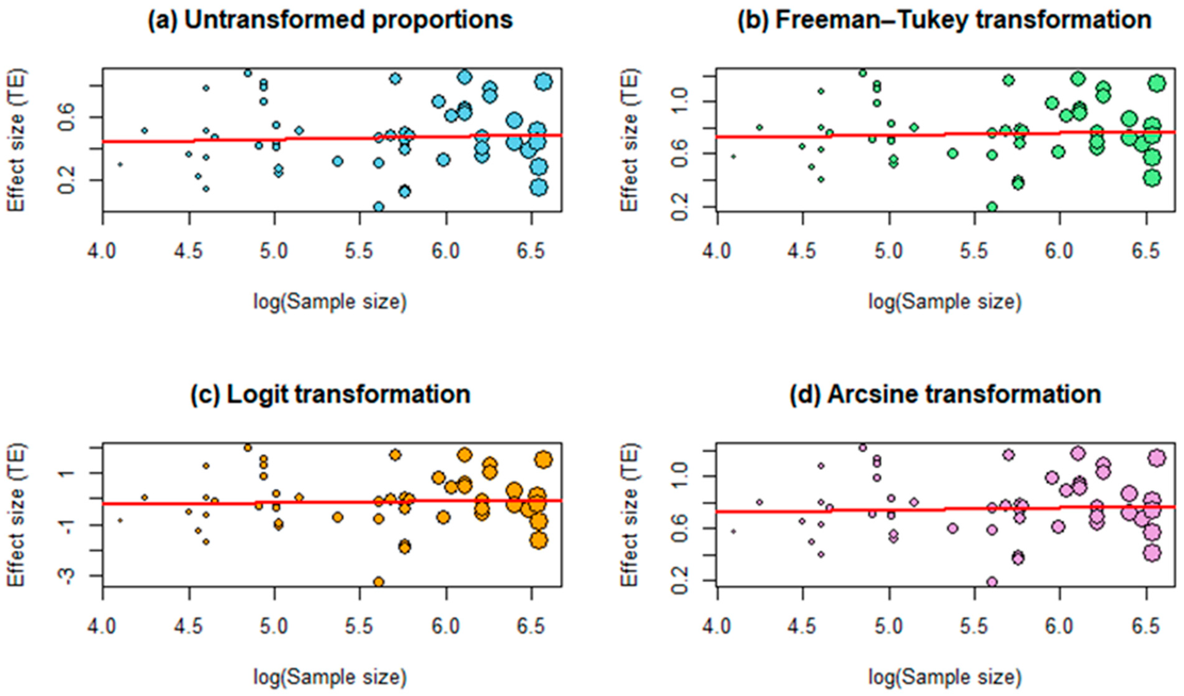
Figure A2.
Monte Carlo simulation results (10,000 iterations) of confidence interval coverage for the four models. The results are displayed for sample sizes of N = 50 (top), N = 200 (middle), and N = 1000 (bottom). The horizontal dashed line indicates the nominal 95% confidence interval coverage.
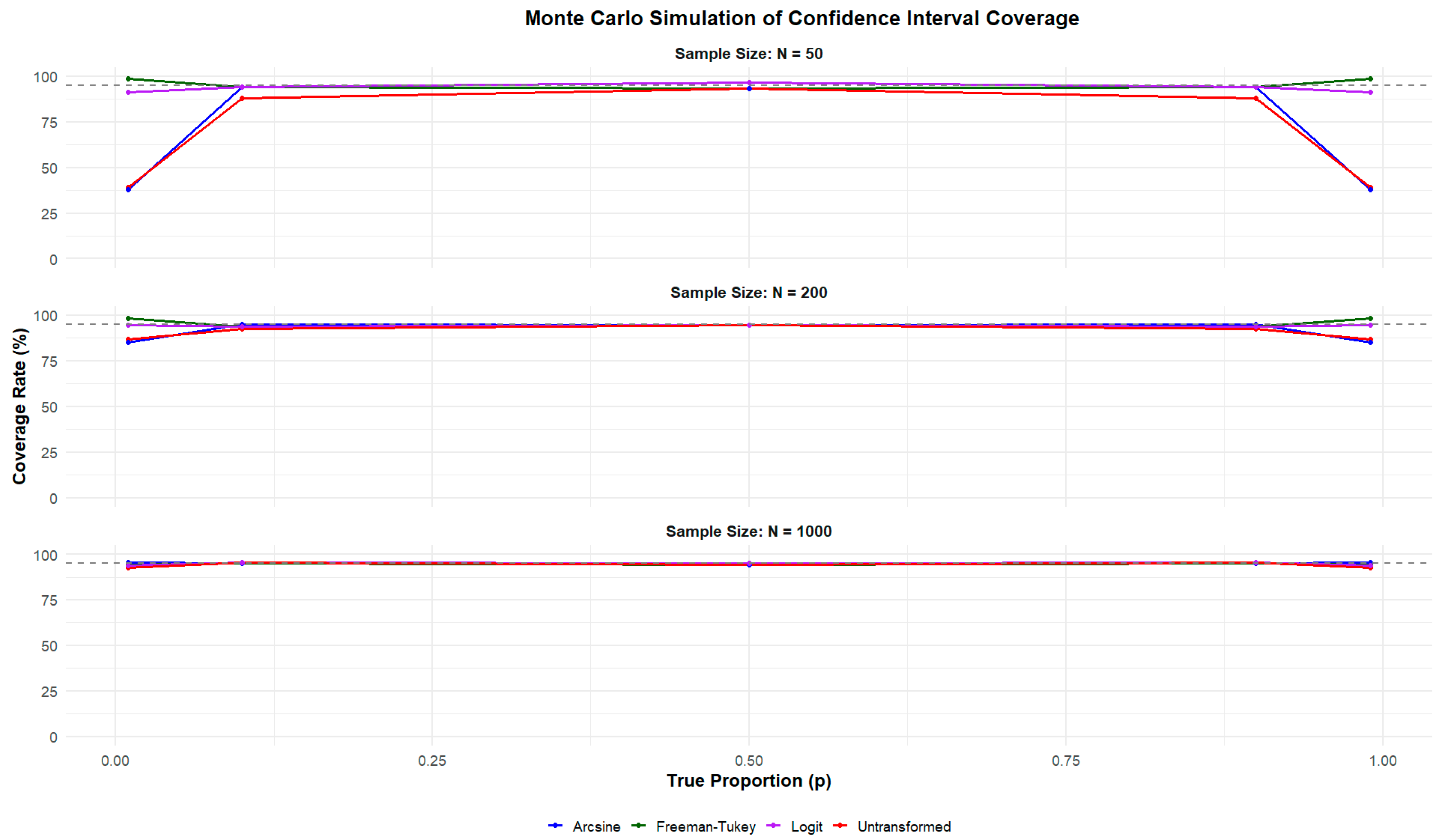
Figure A3.
Visual summary of Bayesian meta-analysis results—Untransformed proportion; (a) Forest plot of untransformed proportions across studies, showing point estimates and 95% confidence intervals. (b) Joint posterior distribution of the overall effect size and heterogeneity (μ, ), with contour shading and credible boundaries. (c) Study-specific posterior distribution for a selected study, illustrating uncertainty around the estimated effect. (d) Posterior predictive distribution for heterogeneity, reflecting expected variability across future studies. The solid blue line represents the estimated effect, the dashed blue lines indicate the corresponding 95% confidence interval, and the green dashed horizontal lines denote the reference (nominal) levels.
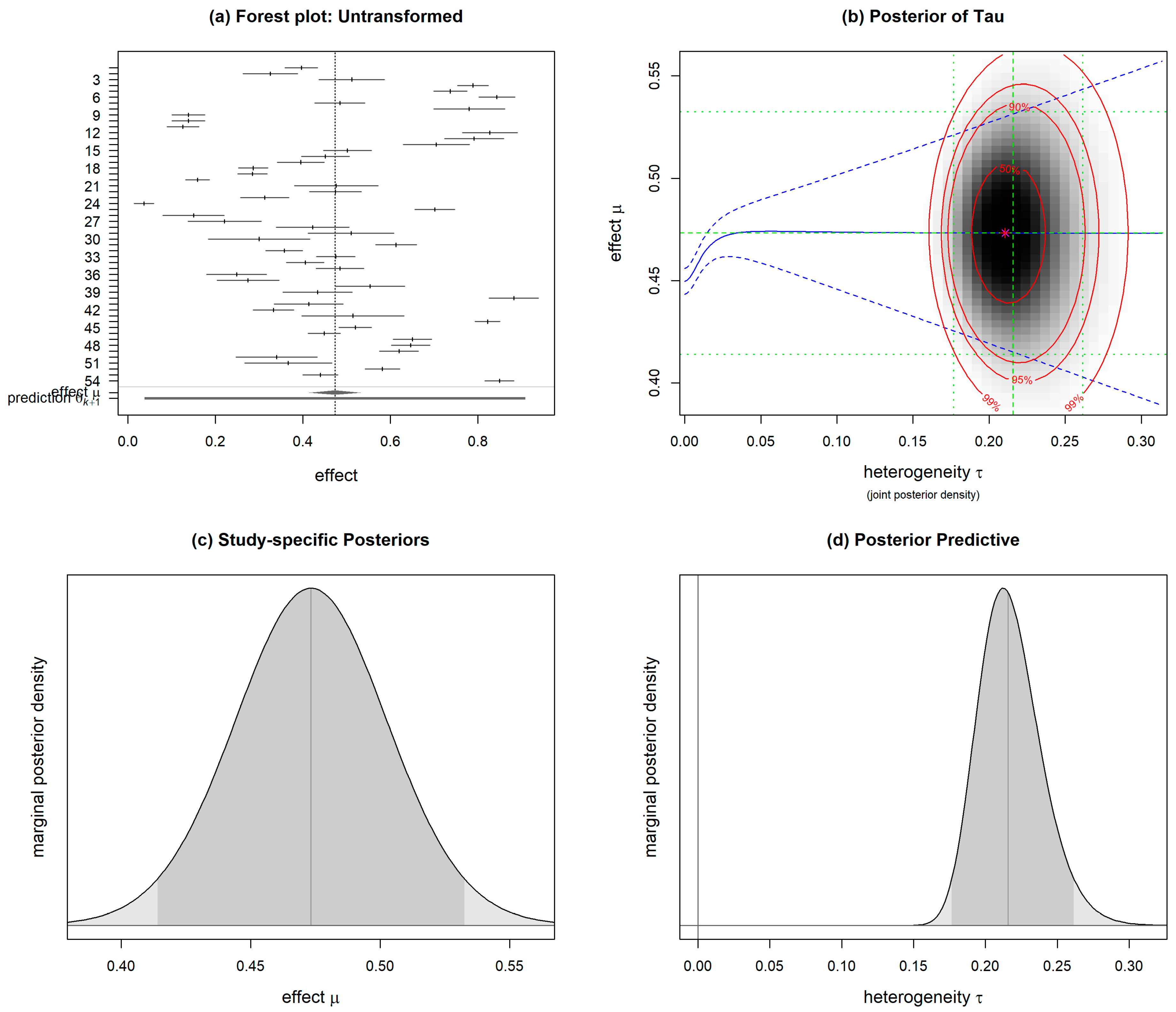
Figure A4.
Visual summary of Bayesian meta-analysis results. (a) Forest plot of Freeman–Tukey doubled arcsine transformation across studies, showing point estimates and 95% confidence intervals. (b) Joint posterior distribution of the overall effect size and heterogeneity (μ, ), with contour shading and credible boundaries. (c) Study-specific posterior distribution for a selected study, illustrating uncertainty around the estimated effect. (d) Posterior predictive distribution for heterogeneity, reflecting expected variability across future studies. The solid blue line represents the estimated effect, the dashed blue lines indicate the corresponding 95% confidence interval, and the green dashed horizontal lines denote the reference (nominal) levels.
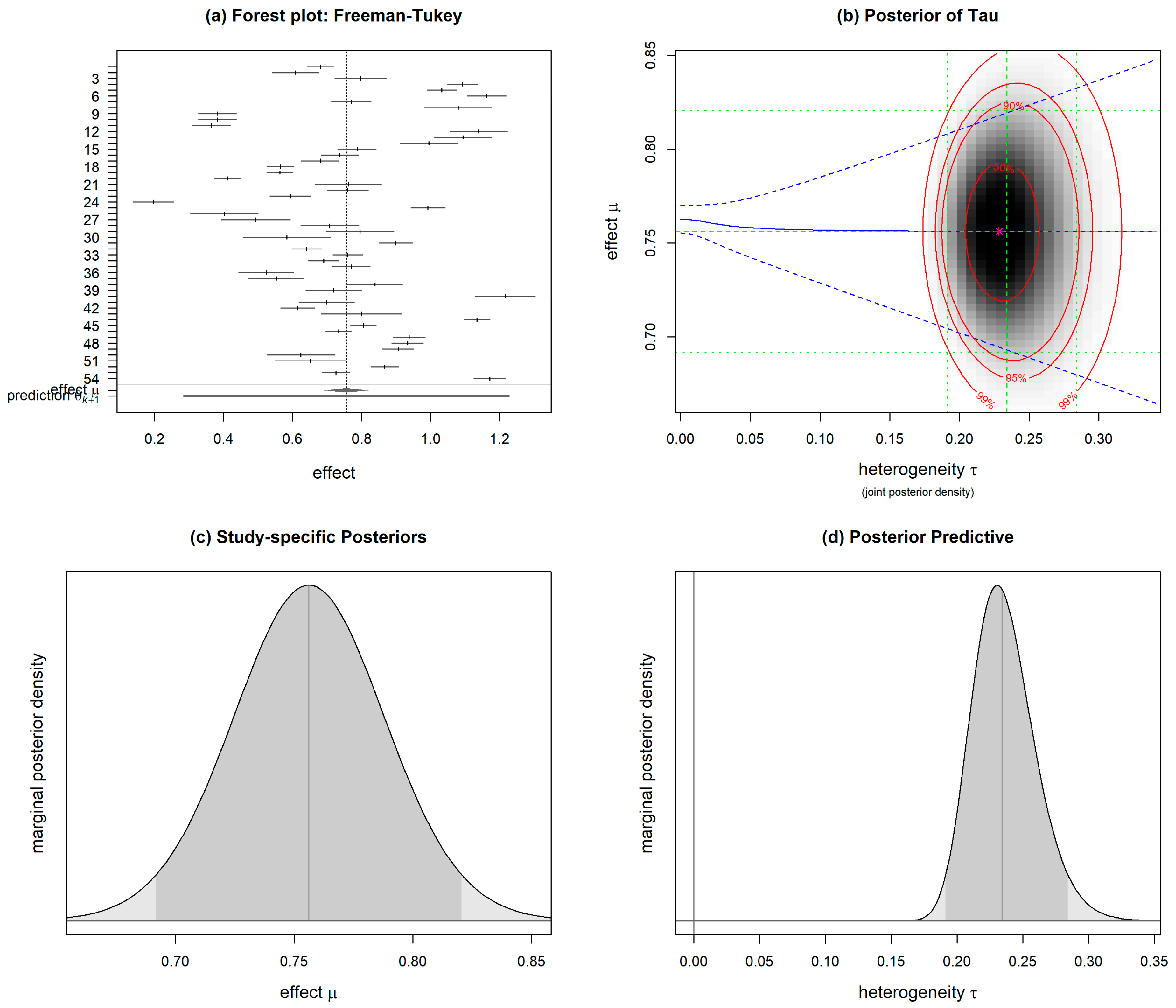
Figure A5.
Visual summary of Bayesian meta-analysis results; (a) Forest plot of Arcsine transformation across studies, showing point estimates and 95% confidence intervals. (b) Joint posterior distribution of the overall effect size and heterogeneity (μ, ), with contour shading and credible boundaries. (c) Study-specific posterior distribution for a selected study, illustrating uncertainty around the estimated effect. (d) Posterior predictive distribution for heterogeneity, reflecting expected variability across future studies. The solid blue line represents the estimated effect, the dashed blue lines indicate the corresponding 95% confidence interval, and the green dashed horizontal lines denote the reference (nominal) levels.
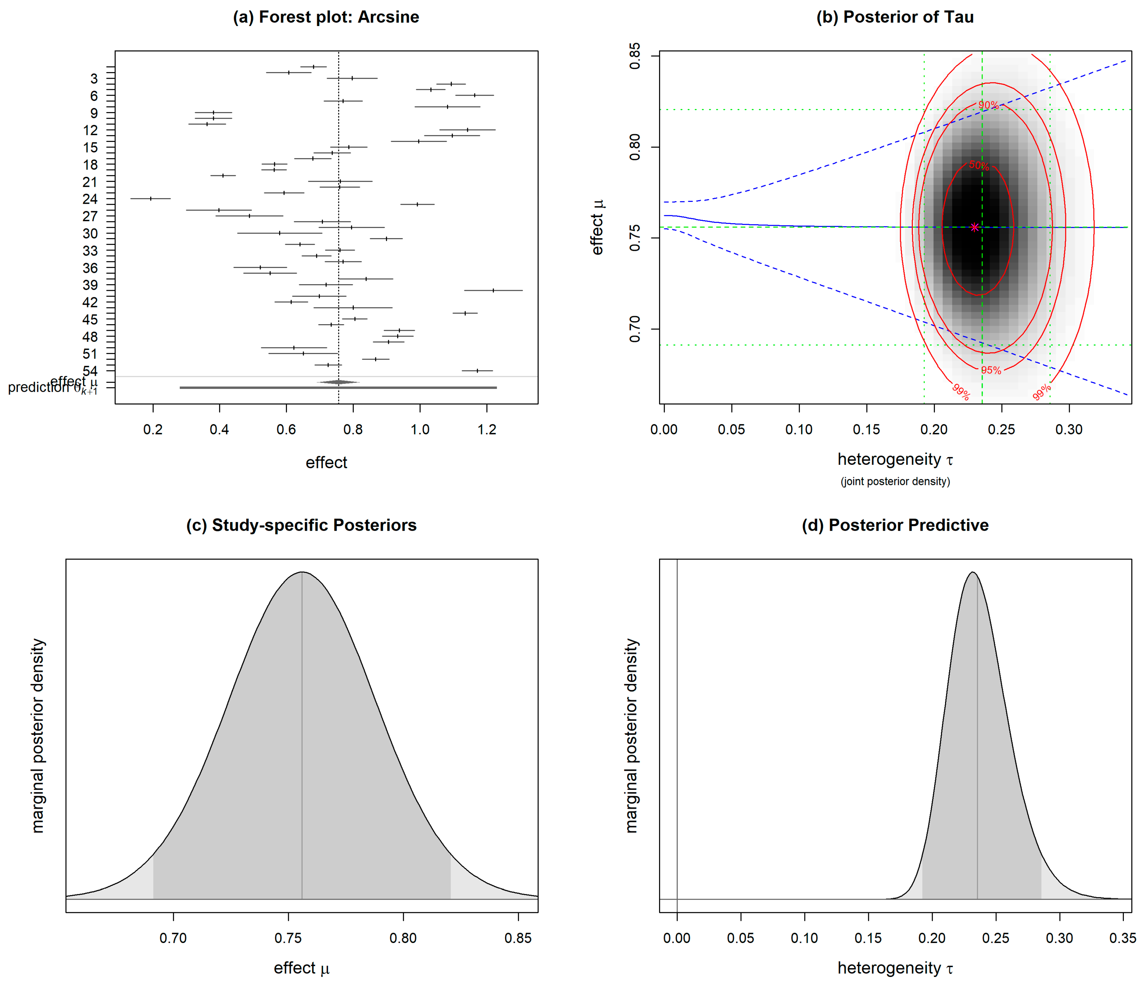
Figure A6.
Visual summary of Bayesian meta-analysis results; (a) Forest plot of Logit transformation across studies, showing point estimates and 95% confidence intervals. (b) Joint posterior distribution of the overall effect size and heterogeneity (μ, ), with contour shading and credible boundaries. (c) Study-specific posterior distribution for a selected study, illustrating uncertainty around the estimated effect. (d) Posterior predictive distribution for heterogeneity, reflecting expected variability across future studies. The solid blue line represents the estimated effect, the dashed blue lines indicate the corresponding 95% confidence interval, and the green dashed horizontal lines denote the reference (nominal) levels.
References
- Astuti, D.; Makaba, S.; Tingginehe, R.M.; Ruru, Y. The determinant factors affecting the event of computer vision syndrome (CVS) on helpdesk employees at PT Telkom Access Papua in 2020. Int. J. Sci. Basic Appl. Res. 2020, 53, 17–34. [Google Scholar]
- Bali, J.; Neeraj, N.; Bali, R. Computer vision syndrome: A review. J. Clin. Ophthalmol. Res. 2014, 2, 61. [Google Scholar] [CrossRef] [Scilit]
- Dimitrijević, V.; Todorović, I.; Viduka, B.; Lavrnić, I.; Viduka, D. Prevalence of computer vision syndrome in computer users: A systematic review and meta-analysis. Vojnosanit. Pregl. 2023, 80, 860–870. [Google Scholar] [CrossRef] [Scilit]
- De-Hita-Cantalejo, C.; García-Pérez, Á.; Sánchez-González, J.-M.M.; Capote-Puente, R.; Sánchez-González, M.C. Accommodative and binocular disorders in preteens with computer vision syndrome: A cross-sectional study. Ann. N. Y. Acad. Sci. 2021, 1492, 73–81. [Google Scholar] [CrossRef] [Scilit]
- Anbesu, E.W.; Lema, A.K. Prevalence of computer vision syndrome: A systematic review and meta-analysis. Sci. Rep. 2023, 13, 1801. [Google Scholar] [CrossRef] [Scilit]
- Negassa Gondol, B.; Shiferawu Areba, A.; Gebremeskel Kanno, G.; Tesfaye Mamo, T. Prevalence of visual and posture-related symptoms of computer vision syndrome among computer user workers of Ethiopian Roads Authority. J. Environ. Occup. Health 2020, 10, 79–90. [Google Scholar]
- Almousa, A.N.; Aldofyan, M.Z.; Kokandi, B.A.; Alsubki, H.E.; Alqahtani, R.S.; Gikandi, P.; Alghaihb, S.G. The impact of the COVID-19 pandemic on the prevalence of computer vision syndrome among medical students in Riyadh, Saudi Arabia. Int. Ophthalmol. 2023, 43, 1275–1283. [Google Scholar] [CrossRef] [Scilit]
- Shah, M.; Saboor, A. Computer vision syndrome: Prevalence and associated risk factors among computer-using bank workers in Pakistan. Turk. J. Ophthalmol. 2022, 52, 295–301. [Google Scholar] [CrossRef] [Scilit]
- Sharma, S.; Kumar Ratha, S. Computer vision syndrome and its risk factors among medical students of a tertiary care centre in Odisha: A cross-sectional study. Int. J. Health Syst. Implement. Res. 2021, 5, 1–8. [Google Scholar]
- Newcombe, R.G. Improved confidence intervals for the difference between binomial proportions based on paired data. Stat. Med. 1998, 17, 2635–2650. [Google Scholar] [CrossRef]
- Barendregt, J.J.; Doi, S.A.; Lee, Y.Y.; Norman, R.E.; Vos, T. Meta-analysis of prevalence. J. Epidemiol. Community Health 2013, 67, 974–978. [Google Scholar] [CrossRef] [Scilit]
- Higgins, J.P.T.; Thompson, S.G. Quantifying heterogeneity in a meta-analysis. Stat. Med. 2002, 21, 1539–1558. [Google Scholar] [CrossRef] [Scilit] [PubMed]
- Freeman, M.F.; Tukey, J.W. Transformations related to the angular and the square root. Ann. Math. Stat. 1950, 21, 607–611. [Google Scholar] [CrossRef] [Scilit]
- Miller, J.J. The inverse of the Freeman–Tukey double arcsine transformation. Am. Stat. 1978, 32, 138. [Google Scholar]
- Viechtbauer, W. Conducting meta-analyses in R with the metafor package. J. Stat. Softw. 2010, 36, 1–48. [Google Scholar] [CrossRef] [Scilit]
- Hamza, T.H.; van Houwelingen, H.C.; Stijnen, T. The binomial distribution of meta-analysis was preferred to model within-study variability. J. Clin. Epidemiol. 2008, 61, 41–51. [Google Scholar] [CrossRef] [Scilit] [PubMed]
- Lin, L.; Chu, H. Meta-analysis of proportions using generalized linear mixed models. Epidemiology 2020, 31, 713–717. [Google Scholar] [CrossRef] [Scilit] [PubMed]
- Lin, L.; Xu, C. Arcsine-based transformations for meta-analysis of proportions: Pros, cons, and alternatives. Health Sci. Rep. 2020, 3, e178. [Google Scholar] [CrossRef] [Scilit]
- Schwarzer, G.; Chemaitelly, H.; Abu-Raddad, L.J.; Rücker, G. Seriously misleading results using inverse of Freeman–Tukey double arcsine transformation in meta-analysis of single proportions. Res. Synth. Methods 2019, 10, 476–483. [Google Scholar] [CrossRef] [Scilit]
- Feder, P.I.; Aume, L.L.; Triplett, C.A.; Simmons, J.E.; Narotsky, M.G. Analysis of proportional data in reproductive and developmental toxicity studies. Birth Defects Res. 2020, 112, 1260–1272. [Google Scholar] [CrossRef] [Scilit]
- Snedecor, G. Statistical Methods, 4th ed.; Iowa State University Press: Ames, IA, USA, 1967. [Google Scholar]
- Jaeger, T.F. Categorical data analysis: Away from ANOVAs. J. Mem. Lang. 2008, 59, 434–446. [Google Scholar] [CrossRef] [Scilit]
- Migliavaca, C.B.; Stein, C.; Colpani, V.; Barker, T.H.; Ziegelmann, P.K.; Munn, Z.; Falavigna, M. Meta-analysis of prevalence: I2 statistic and how to deal with heterogeneity. Res. Synth. Methods 2022, 13, 363–367. [Google Scholar] [CrossRef] [Scilit]
- Röver, C. Bayesian random-effects meta-analysis using the bayesmeta R package. J. Stat. Softw. 2020, 93, 1–51. [Google Scholar] [CrossRef] [Scilit]
- Stijnen, T.; Hamza, T.H.; Özdemir, P. Random effects meta-analysis of event outcome in the framework of the generalized linear mixed model with applications in sparse data. Stat. Med. 2010, 29, 3046–3067. [Google Scholar] [CrossRef] [Scilit]
- Chu, H.; Nie, L.; Chen, Y.; Sun, W. Bivariate random effects models for meta-analysis of comparative studies with binary outcomes. Stat. Methods Med. Res. 2012, 21, 621–633. [Google Scholar] [CrossRef] [Scilit]
- Abudawood, G.A.; Ashi, H.M.; Almarzouki, N.K. Computer vision syndrome among undergraduate medical students in King Abdulaziz University, Jeddah, Saudi Arabia. J. Ophthalmol. 2020, 2020, 2789376. [Google Scholar] [CrossRef] [Scilit]
- Agbonlahor, O. Prevalence and knowledge of computer vision syndrome among working-class adults in FCT, Nigeria. J. Niger. Optom. Assoc. 2019, 21, 49–60. [Google Scholar]
- Al Subaie, M.; Al-Dossari, S.; Bougmiza, M. Computer vision syndrome among mobile phone users in Al-Ahsa, Saudi Arabia. Al-Basar Int. J. Ophthalmol. 2017, 4, 99. [Google Scholar] [CrossRef] [Scilit]
- AlDarrab, A. Awareness and practice regarding use of digital devices and ocular health among Saudi adolescents. Oman J. Ophthalmol. 2022, 15, 73–77. [Google Scholar] [CrossRef] [Scilit] [PubMed]
- Almuqrashi, A.; Al-Noumani, H.; Al-Abri, F.; Al-Hinai, H.; Bani Oraba, H. The prevalence of computer vision syndrome and associated factors among university students in Oman: A cross-sectional study. BMC Public Health 2025, 25, 2668. [Google Scholar] [CrossRef] [Scilit]
- Basnet, A.; Basnet, P.; Karki, P.; Shrestha, S. Computer vision syndrome prevalence and associated factors among medical students. Nepal Med. J. 2018, 1, 29–31. [Google Scholar] [CrossRef] [Scilit]
- Basnet, A.; Pathak, S.B.; Marasini, A.; Pandit, R.; Pradhan, A. Digital eye strain among adults during the COVID-19 pandemic. J. Nepal Med. Assoc. 2022, 60, 22–25. [Google Scholar] [CrossRef] [Scilit]
- Boadi-Kusi, S.B.; Adueming, P.O.W.; Hammond, F.A.; Antiri, E.O. Computer vision syndrome and ergonomic factors among bank workers. Int. J. Occup. Saf. Ergon. 2022, 28, 1219–1226. [Google Scholar] [CrossRef] [Scilit]
- Das, A.; Shah, S.; Adhikari, T.B.; Paudel, B.S.; Sah, S.K.; Das, R.K.; Shah, C.P.; Adhikari, P.G. Computer vision syndrome, musculoskeletal, and stress-related problems among visual display terminal users in Nepal. PLoS ONE 2022, 17, e0268356. [Google Scholar] [CrossRef] [Scilit]
- Demirayak, B.; Yılmaz Tugan, B.; Toprak, M.; Çinik, R. Digital eye strain and its associated factors in children during the COVID-19 pandemic. Indian J. Ophthalmol. 2022, 70, 988–992. [Google Scholar] [CrossRef] [Scilit] [PubMed]
- Gautam, P.S.; Prakash, U.C.; Dangol, S. Knowledge and prevalence of computer vision syndrome among computer operators. J. Nobel Med. Coll. 2020, 9, 45–49. [Google Scholar] [CrossRef] [Scilit]
- Nadir Hadi, K.; Rehman, M.H.; Toru, H.K.; Orakzai, A.A.; Khalid, S.; Iftikhar, B. Assessment of computer vision syndrome in university students in Peshawar: A descriptive cross-sectional study. STETHO 2021, 6, 6–14. [Google Scholar] [CrossRef] [Scilit]
- Iqbal, M.; El-Massry, A.; Elagouz, M.; Elzembely, H. Computer vision syndrome survey among medical students in Sohag University Hospital, Egypt. Ophthalmol. Res. 2018, 8, 1–8. [Google Scholar] [CrossRef] [Scilit]
- Iqbal, M.; Elzembely, H.; Elmassry, A.; Elgharieb, M.; Assaf, A.; Ibrahim, O.; Soliman, A. Computer vision syndrome prevalence and ocular sequelae among medical students. Open Ophthalmol. J. 2021, 15, 156–170. [Google Scholar] [CrossRef] [Scilit]
- Iqbal, M.; Said, O.; Ibrahim, O.; Soliman, A. Visual sequelae of computer vision syndrome: A cross-sectional case-control study. J. Ophthalmol. 2021, 2021, 6614796. [Google Scholar] [CrossRef] [Scilit]
- Kumar, N.; Sharma, N. To determine the prevalence of computer vision syndrome among computer users: A descriptive study. Eur. J. Mol. Clin. Med. 2020, 7, 3933–3938. Available online: https://www.ejmcm.com/archives/volume-7/issue-10/10000 (accessed on 12 September 2025).
- Kumar, S.B. Knowledge regarding computer vision syndrome among medical students. Biomed. Pharmacol. J. 2020, 13, 469–473. [Google Scholar] [CrossRef] [Scilit]
- Logaraj, M.; Madhupriya, V.; Hegde, S. Computer vision syndrome and associated factors among medical and engineering students in Chennai. Ann. Med. Health Sci. Res. 2014, 4, 179. [Google Scholar] [CrossRef] [Scilit] [PubMed]
- Lotfy, N.M.; Shafik, H.M.; Nassief, M. Risk factor assessment of digital eye strain during the COVID-19 pandemic. Med. Hypotheses Discov. Innov. Ophthalmol. 2022, 11, 119–128. [Google Scholar] [CrossRef] [Scilit]
- Noreen, K.; Ali, K.; Aftab, K.; Umar, M. Computer vision syndrome and its associated risk factors among undergraduate medical students during COVID-19. Pak. J. Ophthalmol. 2020, 37, 102–108. [Google Scholar]
- Nwankwo, B.; Mumueh, K.P.; Olorukooba, A.A.; Usman, N.O. Computer vision syndrome among undergraduates in a tertiary institution in northwestern Nigeria. Kanem J. Med. Sci. 2021, 15, 19–26. Available online: https://www.ajol.info/index.php/kjms/article/view/218092 (accessed on 12 September 2025).
- Ranganatha, S.; Jailkhani, S. Prevalence and associated risk factors of computer vision syndrome among computer science students. Galore Int. J. Health Sci. Res. 2019, 4, 10. [Google Scholar]
- Shahid, E.; Burhany, T.; Siddique, W.A.; Fasih, U.; Pak, A.S. Computer use and office ergonomics. Off. Ergon. 2007, 33, 53–64. Available online: https://www.pjo.org.pk/index.php/pjo/article/view/69 (accessed on 12 September 2025).
- Shrestha, P.; Pradhan, P.M.S.; Malla, O.K. Computer vision syndrome among patients attending the outpatient department of ophthalmology. JNMA J. Nepal Med. Assoc. 2020, 58, 721–724. [Google Scholar]
- Al Tawil, L.; Aldokhayel, S.; Zeitouni, L.; Qadoumi, T.; Hussein, S.; Ahamed, S.S. Prevalence of self-reported computer vision syndrome symptoms among university students. Eur. J. Ophthalmol. 2020, 30, 189–195. [Google Scholar]
- Turkistani, A.; Al-Romaih, A.; Alrayes, M.; Al Ojan, A.; Al-Issawi, W. Computer vision syndrome among Saudi population: Prevalence and risk factors. J. Fam. Med. Prim. Care 2021, 10, 2313. [Google Scholar] [CrossRef] [Scilit] [PubMed]
- Uwimana, A.; Ma, C.; Ma, X. Concurrent rising of dry eye and eye strain symptoms among university students during the COVID-19 pandemic. Risk Manag. Healthc. Policy 2022, 15, 2311–2322. [Google Scholar] [CrossRef] [Scilit]
- Verma, S.; Midya, U.; Gupta, S.; Shukla, Y. Prevalence of computer vision syndrome and dry eye in computer operators. TNOA J. Ophthalmic Sci. Res. 2021, 59, 160. [Google Scholar] [CrossRef] [Scilit]
- Viduka, D.; Dragičević, M.; Bašić, A.; Viduka, B.; Lavrnić, I. 21st Century engineering challenges observed through computer vision syndrome. Teh. Vjesn. 2017, 24, 201–205. [Google Scholar]
- Gusti, I.V.; Handayani, A.T. Screening of computer vision syndrome in medical students of Udayana University. Bali J. Ophthalmol. 2018, 2, 28–34. [Google Scholar] [CrossRef] [Scilit]
- Younis, A.; Alsabbagh, L.; Alaraifi, D.; Alsanad, G.; Algrain, A.; AlDihan, R.; Albassam, F. The prevalence and associated factors of self-reported symptoms of computer vision syndrome among high school teachers in Riyadh: A cross-sectional study. J. Nat. Sci. Med. 2022, 5, 292–298. [Google Scholar] [CrossRef] [Scilit]
- Trikalinos, T.A.; Trow, P.; Schmid, C.H. Simulation-based comparison of methods for meta-analysis of proportions and rates. Methods Res. Rep. 2013, 13, 1–98. [Google Scholar]
- Sterne, J.A.C.; Egger, M. Funnel plots for detecting bias in meta-analysis: Guidelines on choice of axis. J. Clin. Epidemiol. 2001, 54, 1046–1055. [Google Scholar] [CrossRef] [Scilit]
- Sterne, J.A.C.; Sutton, A.J.; Ioannidis, J.P.; Terrin, N.; Jones, D.R.; Lau, J.; Carpenter, J.; Rücker, G.; Harbord, R.M.; Schmid, C.H.; et al. Recommendations for examining and interpreting funnel plot asymmetry in meta-analyses of randomized controlled trials. BMJ 2011, 343, d4002. [Google Scholar] [CrossRef] [Scilit]

Disclaimer/Publisher’s Note: The statements, opinions and data contained in all publications are solely those of the individual author(s) and contributor(s) and not of MDPI and/or the editor(s). MDPI and/or the editor(s) disclaim responsibility for any injury to people or property resulting from any ideas, methods, instructions or products referred to in the content. |
© 2026 by the authors. Licensee MDPI, Basel, Switzerland. This article is an open access article distributed under the terms and conditions of the Creative Commons Attribution (CC BY) license.