A Fuzzy Granular K-Means Clustering Method Driven by Gaussian Membership Functions

Abstract

The K-means clustering algorithm is widely applied in various clustering tasks due to its high computational efficiency and simple implementation. However, its performance significantly deteriorates when dealing with non-convex structures, fuzzy boundaries, or noisy data, as it relies on the assumption that clusters are spherical or linearly separable. To address these limitations, this paper proposes a Gaussian membership-driven fuzzy granular K-means clustering method. In this approach, multi-function Gaussian membership functions are used for fuzzy granulation at the single-feature level to generate fuzzy granules, while fuzzy granule vectors are constructed in the multi-feature space. A novel distance metric for fuzzy granules is defined along with operational rules, for which axiomatic proof is provided. This Gaussian-based granulation enables effective modeling of nonlinear separability in complex data structures, leading to the development of a new fuzzy granular K-means clustering framework. Experimental results on multiple public UCI datasets demonstrate that the proposed method significantly outperforms traditional K-means and other baseline methods in clustering tasks involving complex geometric data (e.g., circular and spiral structures), showing improved robustness and adaptability. This offers an effective solution for clustering data with intricate distributions.

1. Introduction

Clustering, as an unsupervised learning technique, aims to partition data objects into groups such that intra-cluster similarity is maximized while inter-cluster similarity is minimized [1,2]. Among clustering algorithms, K-means has been widely adopted in image processing, text analysis, and medical data mining due to its efficiency and ease of implementation [3,4]. However, the clustering performance of K-means is heavily based on the assumption that clusters are spherical, of similar size, and linearly separable—assumptions that are often violated in real-world scenarios. As a result, K-means suffers from degraded accuracy when faced with non-convex structures, fuzzy boundaries, or noise [5].

To enhance the clustering performance on complex data, numerous improvements to K-means have been proposed. For instance, the fuzzy C-means (FCM) algorithm [6] introduces fuzzy membership degrees, allowing each sample to partially belong to multiple clusters, thereby addressing boundary fuzziness to some extent. However, FCM still falls short in capturing nonlinear data structures [7]. Granular computing (GrC), inspired by human cognitive mechanisms for handling complex information, offers a novel modeling paradigm through granulation [8,9,10]. Integrating GrC with clustering—especially in fuzzy environments—promises to improve the robustness and interpretability of clustering algorithms [11,12].

Although the Gaussian nuclear function is widely used, the existing work usually applies it to the nucleated distance or fuzzy membership function at the cluster level. In contrast, our method uses the multi-function Gaussian membership function at the level of characteristic granulation, constructs a structured fuzzy granule vector, and defines granule-based distance measures, which are essentially different from the classic nuclear-based clustering method. By incorporating Gaussian fuzzy membership mechanisms with the principles of granular computing, this method granulates data along each feature dimension using multi-function Gaussian curves, constructs fuzzy granules and fuzzy granule vectors, and establishes a granular distance metric with formally defined operational rules [13,14]. The axiomatic design of the fuzzy granular distance function ensures its theoretical validity. Based on this structure, a novel K-means clustering algorithm is developed that is capable of handling complex data distributions. Experimental results show that the proposed algorithm significantly outperforms traditional K-means and FCM when applied to datasets with non-convex geometries such as spirals and rings [15,16].

The main contributions of this paper include the following:

• A multi-dimensional fuzzy granulation method based on Gaussian membership functions to enhance the nonlinear representability of data structures;
• A set of operational rules and distance metrics for fuzzy granules and granule vectors, with formal axiomatic justification;
• A novel K-means clustering framework that integrates fuzzy granular modeling to improve clustering robustness;
• Comprehensive experiments on benchmark datasets to validate the superiority of the proposed method under complex data distributions.

The remainder of this paper is organized as follows: Section 2 reviews related work; Section 3 and Section 4 introduces the fuzzy granular modeling and distance metric; Section 5 and Section 6 details the proposed fuzzy granular K-means algorithm and its complexity; Section 7 presents the experimental design and analysis; and the final section concludes this paper with discussions on future directions.

2. Related Work

Clustering algorithms, as a cornerstone of unsupervised learning, have evolved significantly in both theoretical and practical contexts. Traditional K-means and its variants, fuzzy clustering approaches, and more recent developments integrating granular computing have each contributed to modeling complex data structures.

2.1. K-Means and Its Improvements

The K-means algorithm is widely used in pattern recognition and data mining due to its fast iterative updates and scalability [1,3]. To overcome limitations such as sensitivity to initialization and vulnerability to local optima, Arthur et al. proposed the K-means++ initialization method [17]. The K-medoids algorithm enhances robustness to outliers by selecting actual data points as centroids [18]. For non-convex clusters, nonlinear methods like Spectral Clustering [19] and density-based methods such as DBSCAN and OPTICS [20,21] have proven effective.

2.2. Clustering and Gaussian Membership Functions

Fuzzy C-means (FCM) is one of the most prominent fuzzy clustering algorithms, allowing each data point to belong to multiple clusters with varying degrees [6]. Researchers have since developed improved versions, such as Weighted FCM (WFCM) [22], Spatially Constrained FCM (SFCM) [23], and Kernel-based FCM (KFCM) [24], to enhance noise tolerance and nonlinear modeling.

In addition to fuzzy clustering, the development trend in clustering research in recent years also includes graph structure learning and matrix decomposition. In particular, spectral clusters benefit from the rapid progress of graph structure learning, which has been comprehensively reviewed in the recent summary of graph learning [25]. Semi-supervised adaptive symmetric non-negative matrix decomposition (ASNMF) also shows strong effectiveness in multi-perspective and noise scenarios [26], further highlighting the development trend in clustering frameworks for structural perception and representation drives.

In addition to fuzzy methods, classic density-based and grid-based clustering algorithms also play a fundamental role in dealing with non-convex structures and noise. DBSCAN [20] can detect clusters of any shape and naturally isolate noise points according to the density criteria, while CLIQUE [27] performs clustering based on subspace networks. The clustering of the grid is effective in high-dimensional data. Density peak clustering (DPC) [28] identifies the cluster center through the maximum value of local density and relative distance, providing a simple and powerful mechanism for the discovery of non-convex clusters. However, these algorithms usually rely on hard allocation and lack the ability to model partial memberships and progressive transitions, which limits their effectiveness in scenarios involving overlapping clusters or uncertain boundaries.

On the other hand, in recent years, people have become more and more interested in the deep clustering method, which combines learning with clustering goals. Representative methods such as deep embedded clustering (DEC) [29] and its variants use deep neural networks to learn nonlinear feature embeddings, which has achieved remarkable performance on complex, large-scale datasets. However, deep clustering methods usually require a large amount of training data, a well-designed network architecture, and high computing costs, which may limit their application in small samples or noise-sensitive scenarios. Unlike density methods and calculation-intensive deep clustering frameworks based on hard distribution, the FGK-means proposed in this paper adopts a lightweight and explainable particle size calculation paradigm. By introducing fuzzy granularity based on Gaussian functions, FGK-means explicitly models some associations and progressive transitions, thus providing a balanced and expressive clustering framework for data with overlapping structures and uncertain boundaries.

Gaussian membership functions are widely used in fuzzy clustering and fuzzy modeling because of their smoothness, differentiability, and powerful ability to capture continuous changes in data distribution. As early basic research points out, the Gaussian function has stable gradient behavior, which is very suitable for a fuzzy learning framework based on optimization [30]. Its bell-shaped structure can effectively model the gradient between clusters, which is especially important for data containing fuzzy or overlapping boundaries [31].

In fuzzy clustering, Gaussian membership modeling has been proven to enhance the robustness of noise and improve the representation of soft boundaries [16]. Recent studies further show that Gaussian kernels and Gaussian membership can achieve more expressive local similarity modeling and improve clustering accuracy in high-dimensional or uncertain environments [32]. Gaussian membership is also widely used in granule calculation frameworks, in which smooth granules composed of Gaussian functions help to improve interpretability and multi-scale representation [33].

Given these advantages, Gauss-based fuzzy representation has become a core component of many modern fuzzy clustering algorithms, especially in scenarios that require smooth decision-making boundaries, explainable granules, and robust uncertainty modeling.

2.3. Granular Computing and Fuzzy–Granular Clustering

Granular computing (GrC) focuses on decomposing complex data into semantically meaningful “granules” to facilitate modeling [8,9]. Recent efforts have combined GrC with clustering methods. The Granular Ball approach proposed by Xia et al. [5,12] enhances boundary representation using fuzzy granules. GRDBSCAN, designed by Suchy et al. [15], introduces granularity layering in density estimation to improve robustness against complex structures.

Fuzzy–granular clustering frameworks have attracted increasing attention. For instance, Zhang et al. proposed a parabolic granule-based fuzzy modeling method [14], while Liu et al. incorporated sparse membership mechanisms to better handle high-dimensional data [16]. Collectively, these studies demonstrate that combining fuzzy and granular modeling significantly enhances clustering performance on datasets with non-convex shapes, fuzziness, and noise.

In summary, although recent studies have achieved considerable progress in combining Gaussian-based fuzzy granulation with clustering methods, there remains a lack of systematic structure modeling and theoretical foundations for distance measurement. This paper’s proposed Gaussian-driven fuzzy granular K-means approach aims to fill this gap.

3. Gaussian Membership Function-Based Fuzzy Granulation

For a dataset $\mathcal{D}$ with N samples, each sample having d feature dimensions, m fuzzy sets are defined on each feature dimension using Gaussian membership functions. The fuzzy granulation process for a single feature involves computing the membership degrees of a sample to each fuzzy set, thereby constructing a fuzzy granule. When applied across multiple feature dimensions, this forms a fuzzy granule vector.

Give a dataset $\mathcal{D}=\{{\mathbf{X}}_1,{\mathbf{X}}_2,\dots ,{\mathbf{X}}_N\}$, where each sample ${\mathbf{X}}_i$ is a d-dimensional feature vector, the fuzzy granulation process proceeds as follows:

$$\begin{array}{c}\hfill {\mathbf{X}}_i=(x_{i1},x_{i2},\dots ,x_{id}),\end{array}$$

(1)

where $x_{ij}$ represents the value of the i-th sample on the j-th feature dimension.

Definition 1.

Let $x_{ij}$ be the feature value of a sample. For each fuzzy set k on the j-th feature dimension, the Gaussian membership function is defined as follows:

$$\begin{array}{c}\hfill {\mu }_{jk}\left(x_{ij}\right)=exp\left(-{\displaystyle \frac{{(x_{ij}-c_{jk})}^2}{2{\delta }_{jk}^2}}\right),\end{array}$$

(2)

where ${\mu }_{jk}\left(x_{ij}\right)$ represents the membership degree of sample ${\mathbf{X}}_i$ to the k-th fuzzy set on feature dimension j; $c_{jk}$ denotes the center of the k-th fuzzy set in the j-th feature dimension; and ${\delta }_{jk}$ indicates the standard deviation of the k-th fuzzy set in the j-th feature dimension.

Definition 2.

The Gaussian fuzzy granulation of feature value $x_{ij}$ yields a set of membership degrees — i.e., a fuzzy granule, which is defined as follows:

$$\begin{array}{c}\hfill P_{ij}=\{{\mu }_{j1}\left(x_{ij}\right),{\mu }_{j2}\left(x_{ij}\right),\dots ,{\mu }_{jm}\left(x_{ij}\right)\},\end{array}$$

(3)

where m is the number of fuzzy sets on the j-th feature dimension.

By applying Gaussian fuzzy granulation to all d feature dimensions of sample ${\mathbf{X}}_i$, we obtain d fuzzy granules, which form a fuzzy granule vector:

$$\begin{array}{c}\hfill {\mathbf{V}}_i=(P_{i1},P_{i2},\dots ,P_{id}),\end{array}$$

(4)

or equivalently

$$\begin{array}{c}\hfill {\mathbf{V}}_i=(\{{\mu }_{11}\left(x_{i1}\right),{\mu }_{12}\left(x_{i1}\right),\dots ,{\mu }_{1m}\left(x_{i1}\right)\},\{{\mu }_{21}\left(x_{i2}\right),{\mu }_{22}\left(x_{i2}\right),\\ \hfill \dots ,{\mu }_{2m}\left(x_{i2}\right)\},\dots ,\{{\mu }_{d1}\left(x_{id}\right),{\mu }_{d2}\left(x_{id}\right),\dots ,{\mu }_{dm}\left(x_{id}\right)\}).\end{array}$$

(5)

After applying Gaussian function-based fuzzification to each sample ${\mathbf{X}}_i$ in the dataset $\mathcal{D}$, the resulting set of fuzzy granular vectors $\{V_1,V_2,\dots ,V_N\}$ represents the fuzzy membership distribution of dataset $\mathcal{D}$, expressed as follows:

$$\begin{array}{c}\hfill \mathcal{V}=\left\{{\mathbf{V}}_i=\left({\left\{{\mu }_{jk}\left(x_{ij}\right)\mid k=1,2,\dots ,m\right\}}_{j=1}^d\right)|i=1,2,\dots ,N\right\},\end{array}$$

(6)

where $i=1,2,\dots ,N$ denotes each sample in the dataset; $j=1,2,\dots ,d$ denotes the feature dimensions of each sample; and $k=1,2,\dots ,m$ denotes the number of fuzzy sets in each feature dimension.

Example 1.

As shown in Table 1, the weather dataset includes two dimensions: temperature and humidity. In this example, the centers and standard deviations of the Gaussian fuzzy sets are manually specified according to the value ranges of the features, aiming to illustrate the fuzzy granulation process. In practical applications, these parameters can be automatically derived from data statistics, as described in Section 5. The fuzzy sets for temperature are defined as Low, Medium, and High, with Gaussian membership function parameters as follows: Low (center $c=10$, standard deviation $\sigma =5$), Medium (center $c=25$, standard deviation $\sigma =5$), and High (center $c=35$, standard deviation $\sigma =5$). The fuzzy sets for humidity are also defined as Low, Medium, and High, with Gaussian membership function parameters as follows: Low (center $c=30$, standard deviation $\sigma =10$), Medium (center $c=60$, standard deviation $\sigma =10$), and High (center $c=90$, standard deviation $\sigma =10$).

Table 1. The weather dataset.

Time	Temperature (°C)	Humidity (%)
08:00	20	40
12:00	25	55
16:00	30	65

For each sample, compute the membership degrees for temperature x and humidity y, perform Gaussian fuzzy granulation, and construct the corresponding fuzzy granules and fuzzy granule vectors. The results are shown in Table 2.

Table 2. Fuzzy granulation results of weather dataset.

Time	Temperature Fuzzy Granule	Humidity Fuzzy Granule	Fuzzy Granule Vectors
08:00	$\{0.14,0.61,0.01\}$	$\{0.61,0.14,0\}$	$\left(\right\{0.14,0.61,0.01\},\{0.61,0.14,0\left\}\right)$
12:00	$\{0.01,1,0.14\}$	$\{0.04,0.88,0.002\}$	$\left(\right\{0.01,1,0.14\},\{0.04,0.88,0.002\left\}\right)$
16:00	$\{0,0.61,0.61\}$	$\{0.002,0.88,0.04\}$	$\left(\right\{0,0.61,0.61\},\{0.002,0.88,0.04\left\}\right)$

For temperature $x=20$, the Gaussian fuzzy granulation is

$$\begin{array}{c}\hfill {\mu }_{\mathit{low}}\left(20\right)=exp\left(-{\displaystyle \frac{{(20-10)}^2}{2\times 5^2}}\right)=0.14,\\ \hfill {\mu }_{\mathit{medium}}\left(20\right)=exp\left(-{\displaystyle \frac{{(20-25)}^2}{2\times 5^2}}\right)=0.61,\\ \hfill {\mu }_{\mathit{high}}\left(20\right)=exp\left(-{\displaystyle \frac{{(20-35)}^2}{2\times 5^2}}\right)=0.01.\end{array}$$

Then the constructed temperature fuzzy granule is $P_{11}=\{0.14,0.61,0.01\}$.

For humidity $y=40$, the Gaussian fuzzy granulation is

$$\begin{array}{c}\hfill {\mu }_{\mathit{low}}\left(40\right)=exp\left(-{\displaystyle \frac{{(40-30)}^2}{2\times {10}^2}}\right)=0.61,\\ \hfill {\mu }_{\mathit{medium}}\left(40\right)=exp\left(-{\displaystyle \frac{{(40-60)}^2}{2\times {10}^2}}\right)=0.14,\\ \hfill {\mu }_{\mathit{high}}\left(40\right)=exp\left(-{\displaystyle \frac{{(40-90)}^2}{2\times {10}^2}}\right)\approx 0.\end{array}$$

Thus, the constructed humidity fuzzy granule is

$$\begin{array}{c}\hfill P_{12}=\{0.61,0.14,0\}.\end{array}$$

4. Granular Representation and Distance Metrics

The proposed fuzzy granular K-means clustering algorithm relies on a distance metric to quantify the dissimilarity between samples in the fuzzy granular space. This section defines the three metrics—Euclidean, Manhattan, and cosine distance—adapted for fuzzy granular vectors. These metrics serve as the foundation for measuring the proximity between data points during the clustering process.

Given two d-dimensional samples $\mathbf{X}=(x_1,x_2,\dots ,x_d)$ and $\mathbf{Y}=(y_1,y_2,\dots ,y_d)$, let their corresponding fuzzy granular vectors be $\mathbf{V}=(P_1,P_2,\dots ,P_d)$ and $\mathbf{U}=(Q_1,Q_2,\dots ,Q_d)$. Here, $P_i=\{{\mu }_{i1}\left(x_i\right),\dots ,{\mu }_{im}\left(x_i\right)\}$ and $Q_i=\{{\eta }_{i1}\left(y_i\right),\dots ,{\eta }_{im}\left(y_i\right)\}$ are the fuzzy granules on the i-th feature. The dissimilarity between V and U can be calculated as follows.

Definition 3.

For two fuzzy granular vectors $\mathbf{V}=(P_1,P_2,\dots ,P_d)$ and $\mathbf{U}=(Q_1,Q_2,\dots ,Q_d)$, the Euclidean distance between them is calculated as follows:

$$\begin{array}{c}\hfill {\mathrm{d}}_{\mathit{Euclid}}(\mathbf{V},\mathbf{U})=\sqrt{{\displaystyle \sum _{i=1}^d}{\displaystyle \sum _{j=1}^m}{\left({\mu }_{ij}\left(x_i\right)-{\eta }_{ij}\left(y_i\right)\right)}^2}.\end{array}$$

(7)

Definition 4.

The Manhattan distance between fuzzy granular vectors is defined as follows:

$$\begin{array}{c}\hfill {\mathrm{d}}_{\mathit{Manhattan}}(\mathbf{V},\mathbf{U})=\sum _{i=1}^d\sum _{j=1}^m\left|{\mu }_{ij}\left(x_i\right)-{\eta }_{ij}\left(y_i\right)\right|.\end{array}$$

(8)

The Euclidean distance between fuzzy granular vectors is the sum of squared differences of membership degrees across all fuzzy sets in each feature dimension—a geometric distance. The Manhattan distance between fuzzy granular vectors is the sum of absolute differences of membership degrees across all fuzzy sets in each feature dimension.

Definition 5.

The cosine distance between fuzzy granular vectors is defined as follows:

$$\begin{array}{c}\hfill {\mathrm{d}}_{\mathit{Cosine}}(\mathbf{V},\mathbf{U})=1-{\displaystyle \frac{{\sum }_{i=1}^d{\sum }_{j=1}^m{\mu }_{ij}\left(x_i\right){\eta }_{ij}\left(y_i\right)}{\sqrt{{\sum }_{i=1}^d{\sum }_{j=1}^m{\mu }_{ij}^2\left(x_i\right)}\sqrt{{\sum }_{i=1}^d{\sum }_{j=1}^m{\eta }_{ij}^2\left(y_i\right)}}}.\end{array}$$

(9)

Cosine distance measures the directional similarity between two fuzzy granular vectors.

Theorem 1.

The Euclidean distance between two fuzzy granule vectors is a valid distance metric, satisfying the following three properties:

1. 

Non-negativity, ${\mathrm{d}}_{\mathit{Euclid}}(\mathbf{V},\mathbf{U})\ge 0$;

2. 

Symmetry, ${\mathrm{d}}_{\mathit{Euclid}}(\mathbf{V},\mathbf{U})={\mathrm{d}}_{\mathit{Euclid}}(\mathbf{U},\mathbf{V})$;

3. 

Triangle inequality, ${\mathrm{d}}_{\mathit{Euclid}}(\mathbf{V},\mathbf{T})+{\mathrm{d}}_{\mathit{Euclid}}(\mathbf{T},\mathbf{U})\ge {\mathrm{d}}_{\mathit{Euclid}}(\mathbf{V},\mathbf{U})$.

Theorem 2.

The Manhattan distance between two fuzzy granule vectors is a distance metric that satisfies the following three properties:

1. 

Non-negativity, ${\mathrm{d}}_{\mathit{Manhattan}}(\mathbf{V},\mathbf{U})\ge 0$;

2. 

Symmetry, ${\mathrm{d}}_{\mathit{Manhattan}}(\mathbf{V},\mathbf{U})={\mathrm{d}}_{\mathit{Manhattan}}(\mathbf{U},\mathbf{V})$;

3. 

Triangle inequality, ${\mathrm{d}}_{\mathit{Manhattan}}(\mathbf{V},\mathbf{T})+{\mathrm{d}}_{\mathit{Manhattan}}(\mathbf{T},\mathbf{U})\ge {\mathrm{d}}_{\mathit{Manhattan}}(\mathbf{V},\mathbf{U})$.

Theorem 3.

The cosine distance between two fuzzy granule vectors is also a distance metric that satisfies the following three properties:

1. 

Non-negativity, ${\mathrm{d}}_{\mathit{Cosine}}(\mathbf{V},\mathbf{U})\ge 0$;

2. 

Symmetry, ${\mathrm{d}}_{\mathit{Cosine}}(\mathbf{V},\mathbf{U})={\mathrm{d}}_{\mathit{Cosine}}(\mathbf{U},\mathbf{V})$;

3. 

Triangle inequality, ${\mathrm{d}}_{\mathit{Cosine}}(\mathbf{V},\mathbf{T})+{\mathrm{d}}_{\mathit{Cosine}}(\mathbf{T},\mathbf{U})\ge {\mathrm{d}}_{\mathit{Cosine}}(\mathbf{V},\mathbf{U})$.

Informally speaking, the proposed granule size distance emphasizes the characteristic consistency under fuzzy membership. When two points have a high degree of membership to the same Gaussian component, their granule size distance will be reduced so that the metric can better distinguish clusters with overlapping clear boundaries.

5. Fuzzy Granular K-Means

By computing the membership degree of each sample in every feature dimension using Gaussian membership functions, the data samples are granulated into fuzzy granule vectors. Then, the distance measures between fuzzy granule vectors are used for iterative clustering, thereby realizing the Gaussian fuzzy granule K-means clustering algorithm.

Unlike the traditional fuzzy clustering method, which relies on random initialization of membership matrices, the Gaussian membership function in FGK-means is constructed based on the statistical characteristic determinism of each feature dimension. Specifically, the center and standard deviation of the Gaussian function are derived from the mean and standard deviation of the data, thus avoiding the instability caused by random initialization. The ambiguity introduced by fuzzy membership is not regarded as an uncertainty that needs to be eliminated, but as valuable information that reflects the gradual transition between clusters. This ambiguity is further aggregated into fuzzy granularity vectors, thus improving the robustness of noise and overlapping boundaries. In addition to the predefined cluster number K, the FGK-means algorithm does not introduce additional class selection parameters, which is consistent with the standard K-means clustering algorithm.

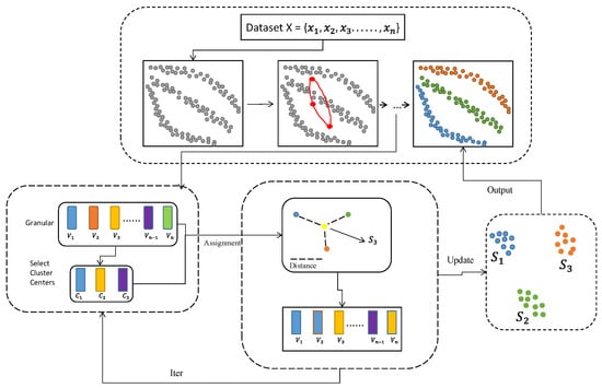
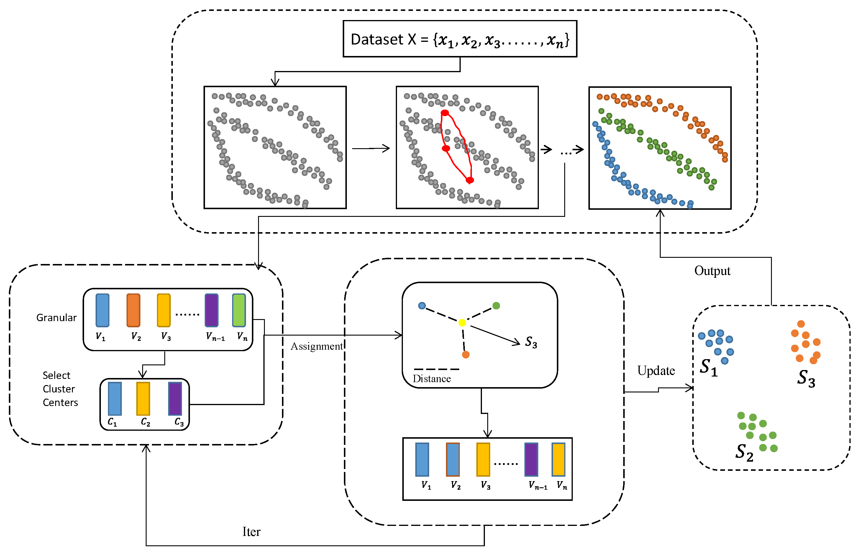
The specific principle is illustrated in Figure 1 and explained as follows:

Figure 1. Flowchart of the fuzzy granular K-means clustering.

5.1. Gaussian Fuzzy Granulation

Consider a dataset $\mathcal{D}=\{{\mathbf{X}}_1,{\mathbf{X}}_2,\dots ,{\mathbf{X}}_N\}$, where each data point ${\mathbf{X}}_i$ is a d-dimensional vector, ${\mathbf{X}}_i=(x_{i1},x_{i2},\dots ,x_{id})$, and a predefined number of clusters K.

Initialization of Gaussian Fuzzy Parameters: For each feature dimension j, the parameters of the m Gaussian fuzzy sets are randomly initialized based on the statistical properties of the data. Specifically, the centers of the Gaussian membership functions are independently sampled from the interval $({\mu }_j-{\sigma }_j,{\mu }_j+{\sigma }_j)$, where ${\mu }_j$ and ${\sigma }_j$ denote the mean and standard deviation of the j-th feature, respectively. The corresponding standard deviations are randomly generated within the range $(0.5{\sigma }_j,1.5{\sigma }_j)$. This strategy introduces randomness into the fuzzy granulation process and enhances the diversity of the generated fuzzy granules. The detailed procedure for this granulation process is summarized in Algorithm 1.

Gaussian Granulation: Each data point ${\mathbf{X}}_i$ is granulated using a Gaussian fuzzy set to obtain its fuzzy granule vector ${\mathbf{V}}_i$. The specific granulation formula is

$$\begin{array}{c}\hfill {\mathbf{V}}_i=(\{{\mu }_{11}\left(x_{i1}\right),{\mu }_{12}\left(x_{i1}\right),\dots ,{\mu }_{1m}\left(x_{i1}\right)\},\{{\mu }_{21}\left(x_{i2}\right),{\mu }_{22}\left(x_{i2}\right),\dots ,{\mu }_{2m}\left(x_{i2}\right)\},\dots ,\\ \hfill \{{\mu }_{d1}\left(x_{id}\right),{\mu }_{d2}\left(x_{id}\right),\dots ,{\mu }_{dm}\left(x_{id}\right)\})\end{array}$$

where ${\mu }_{jm}\left(x_{ij}\right)$ is the Gaussian membership of the m-th fuzzy set on the j-th feature dimension of a sample.

Random Initialization of Cluster Centers: Randomly select K fuzzy granule vectors as the initial cluster centers, denoted as $\{{\mathbf{C}}_1,{\mathbf{C}}_2,\dots ,{\mathbf{C}}_K\}$, where ${\mathbf{C}}_K$ is the center granule vector of the k-th cluster.

5.2. Assignment Step

For each fuzzy granule vector ${\mathbf{V}}_i$, we compute its distance to each cluster center ${\mathbf{C}}_k$ and assign ${\mathbf{V}}_i$ to the nearest cluster $S_k$. The Euclidean distance between the fuzzy granule vector ${\mathbf{V}}_i$ and the cluster center ${\mathbf{C}}_k$ is calculated using the formula

$$d({\mathbf{V}}_i,{\mathbf{C}}_k)=\sqrt{{\displaystyle \sum _{j=1}^d}{\displaystyle \sum _{l=1}^m}{\left({\mu }_{jl}\left(x_{ij}\right)-{\mu }_{jl}\left(c_{kj}\right)\right)}^2},$$

where $c_{kj}$ denotes the center value of cluster ${\mathbf{C}}_k$ on the j-th dimension.

Assign ${\mathbf{V}}_i$ to the cluster with the minimum distance:

$$k=\underset{k\in \{1,2,\dots ,K\}}{arg\; min}d({\mathbf{V}}_i,{\mathbf{C}}_k).$$

5.3. Update Step

After each iteration, recalculate the center granule vector ${\mathbf{C}}_k$ for each cluster $S_k$. The update formula is

$${\mu }_{jl}\left(c_{kj}\right)={\displaystyle \frac{1}{|S_k|}}\sum _{{\mathbf{V}}_i\in S_k}{\mu }_{jl}\left(x_{ij}\right),$$

where ${\mu }_{jl}\left(c_{kj}\right)$ is the membership degree of the l-th fuzzy set on the j-th feature dimension in cluster $S_k$, and $|S_k|$ is the number of data points in cluster $S_k$.

5.4. Stopping Condition

Repeat the assignment and update steps until one of the following stopping conditions is met:

• The cluster center vectors $\{{\mathbf{C}}_1,{\mathbf{C}}_2,\dots ,{\mathbf{C}}_K\}$ no longer change.
• The maximum number of iterations is reached.

5.5. Objective Function

The goal of the clustering algorithm is to minimize the sum of squared distances between all fuzzy granule vectors and their corresponding cluster centers. The objective function is

$$J=\sum _{k=1}^K\sum _{{\mathbf{V}}_i\in S_k}d{({\mathbf{V}}_i,{\mathbf{C}}_k)}^2,$$

where J represents the total distance of all fuzzy granule vectors to their cluster centers, which is the optimization target of the clustering.

Algorithm 1 Fuzzy granulation

Require: $\mathcal{D}=\{{\mathbf{X}}_1,{\mathbf{X}}_2,\dots ,{\mathbf{X}}_N\}$, where ${\mathbf{X}}_i\in {\mathbb{R}}^d$ Ensure: $\mathcal{V}=\{{\mathbf{V}}_1,{\mathbf{V}}_2,\dots ,{\mathbf{V}}_N\}$ 1: for each dimension $j=1$ to d do 2:       Compute global standard deviation ${\sigma }_j$ from $\{x_{1j},x_{2j},\dots ,x_{Nj}\}$ 3: end for 4: for each sample ${\mathbf{X}}_i\in \mathcal{D}$ do 5:       for each dimension $j=1$ to d do 6:             Set ${\mu }_j\leftarrow x_{ij}$ and ${\sigma }_j$ as the standard deviation from step 2 7:             $V_i\left[j\right]\leftarrow ({\mu }_j,{\sigma }_j)$ 8:       end for 9:       Append ${\mathbf{V}}_i$ to $\mathcal{V}$ 10: end for 11: return $\mathcal{V}$

Based on the constructed fuzzy granule vectors in Table 2, the following steps illustrate how the proposed FGK-means performs distance computation and clustering.

Example 2.

Assume that the number of clusters is set to $K=2$, and the initial cluster centers are selected from the fuzzy granule vectors.

Let ${\mathbf{V}}_1=(P_{11},P_{12})$ and ${\mathbf{V}}_2=(P_{21},P_{22})$ denote the fuzzy granule vectors corresponding to 08:00 and 12:00, respectively, where

$$P_{11}=\{0.14,0.61,0.01\},P_{12}=\{0.61,0.14,0\},$$

$$P_{21}=\{0.01,1,0.14\},P_{22}=\{0.04,0.88,0.002\}.$$

According to the proposed granule-based distance, the granule-based distance in this example is instantiated using the ${\mathrm{d}}_{\mathit{Manhattan}}$ (Manhattan distance) between membership degrees, and the distance between two fuzzy granule vectors is defined as

$${\mathrm{d}}_{\mathit{Manhattan}}({\mathbf{V}}_1,{\mathbf{V}}_2)=({\mathrm{d}}_{\mathit{Manhattan}}(P_{11},P_{21}),{\mathrm{d}}_{\mathit{Manhattan}}(P_{12},P_{22})).$$

For the temperature fuzzy granules $P_{11}$ and $P_{21}$, the distance is computed as

$${\mathrm{d}}_{\mathit{Manhattan}}(P_{11},P_{21})=|0.14-0.01|+|0.61-1|+|0.01-0.14|=0.13+0.39+0.13=0.65.$$

Similarly, for the humidity fuzzy granules $P_{12}$ and $P_{22}$, the distance is computed as

$${\mathrm{d}}_{\mathit{Manhattan}}(P_{12},P_{22})=|0.61-0.04|+|0.14-0.88|+|0-0.002|=0.57+0.74+0.002=1.312.$$

Thus, the distance between ${\mathbf{V}}_1$ and ${\mathbf{V}}_2$ is

$${\mathrm{d}}_{\mathit{Manhattan}}({\mathbf{V}}_1,{\mathbf{V}}_2)=(0.65,1.312).$$

Based on the computed granule-based distances, each fuzzy granule vector is assigned to the nearest cluster center according to the minimum distance criterion. Specifically, the fuzzy granule vectors corresponding to 08:00 and 12:00 are selected as the initial cluster centers. In contrast, the remaining granule vector at 16:00 is assigned to the cluster whose center yields the smallest Manhattan granule distance. Consequently, the initial clustering result consists of two clusters, where the first cluster contains the granule vector at 08:00 and the second cluster contains the granule vectors at 12:00 and 16:00.

After the assignment step, the cluster centers are updated by averaging the membership degrees of all fuzzy sets within each feature dimension, following the update rule in Algorithm 2. The assignment and update steps are iteratively performed until the clustering results converge or the maximum number of iterations is reached.

Algorithm 2 Fuzzy granular K-means

Require:         $\mathcal{V}=\{{\mathbf{V}}_1,{\mathbf{V}}_2,\dots ,{\mathbf{V}}_N\}$, K, MaxIter Ensure:         $S=\{S_1,S_2,\dots ,S_K\}$ 1: Randomly select K vectors from $\mathcal{V}$ as initial cluster centers $\{{\mathbf{C}}_1,{\mathbf{C}}_2,\dots ,{\mathbf{C}}_K\}$ 2: $iter\leftarrow 0$ 3: repeat 4:       for $k=1$ to  K do 5:             $S_k\leftarrow \varnothing$ 6:       end for 7:       for each ${\mathbf{V}}_i\in \mathcal{V}$ do 8:             Calculate distance to all centers: 9:             for $k=1$ to K do 10:                  $d({\mathbf{V}}_i,C_k)\leftarrow \sqrt{{\sum }_{j=1}^d\left[{({\mu }_{ij}-{\mu }_{kj})}^2+{({\sigma }_{ij}-{\sigma }_{kj})}^2\right]}$ 11:            end for 12:            Assign ${\mathbf{V}}_i$ to nearest ${\mathbf{C}}_k$: $argmi{n}_{k}d({\mathbf{V}}_i,{\mathbf{C}}_k)$ 13:       end for 14:       for $k=1$ to K do 15:             ${\mathbf{C}}_k\leftarrow \mathrm{mean}\mathrm{of}\{{\mathbf{V}}_i\mid i\in S_k\}$ 16:       end for 17:       $iter\leftarrow iter+1$ 18: until centers converge or $iter\ge \mathrm{MaxIter}$ 19: return $\{S_1,S_2,\dots ,S_K\}$

Example 2 demonstrates the complete FGK-means clustering procedure, from fuzzy granule vector construction to distance computation and cluster assignment. The clustering performance values reported in the experimental section are obtained by applying this procedure to the entire dataset.

6. Algorithm Complexity

The computational complexity of the proposed FGK-means algorithm is determined by two factors: (i) the Gaussian-based fuzzy granulation applied to each feature and (ii) the iterative clustering process based on granule distance.

Set N to the number of samples, d to the number of features, K to the number of clusters, T to the number of iterations, and m to the number of Gaussian-dependent functions used for single-feature granularization. Since m is a smaller constant determined by the fuzzy granulation process design, the overall scalability of the algorithm mainly depends on N, d, and K.

In the initialization stage, each numerical feature is converted into an m-dimensional fuzzy granule. This granulation process requires $\mathcal{O}\left(Ndm\right)$ operations and is performed only once. In the subsequent clustering stage, the granulation distance between each sample and each cluster prototype is calculated by evaluating the membership differences of all features. Such a single calculation requires $\mathcal{O}\left(dm\right)$ operations, so the iteration cost of each iteration is $\mathcal{O}\left(NKdm\right)$. The time complexity of updating the fuzzy granule prototype through the membership average is linearly related to N and d and does not dominate the total cost. Therefore, the overall time complexity of FGK-means is

$$\mathcal{O}\left(Ndm\right)+\mathcal{O}\left(TNKdm\right),$$

Gradually, it is dominated by $\mathcal{O}\left(TNKdm\right)$. When $m=1$, the algorithm naturally degenerates into the standard K-means algorithm.

In terms of memory use, FGK-means needs to store the fuzzy granule vectors and clustered granule prototypes of all samples and requires the space of $\mathcal{O}\left(Ndm\right)$ and $\mathcal{O}\left(Kdm\right)$, respectively. Therefore, its total spatial complexity is $\mathcal{O}\left(Ndm\right)$, which is linearly related to the size of the dataset.

In contrast, the time complexity of standard K-means is $\mathcal{O}\left(TNKd\right)$, the spatial complexity is $\mathcal{O}\left(Nd\right)$, and the time complexity of fuzzy C-means (FCM) is also $\mathcal{O}\left(TNKd\right)$.

For comparison, the time complexities of classical clustering algorithms are summarized in Table 3.

Table 3. Time and space complexity comparison of clustering algorithms.

Algorithm	Time Complexity	Space Complexity
K-means	$\mathcal{O}\left(TNKd\right)$	$\mathcal{O}\left(Nd\right)$
FCM	$\mathcal{O}\left(TNKd\right)$	$\mathcal{O}\left(Nd\right)$
FGK-means	$\mathcal{O}\left(Ndm\right)+\mathcal{O}\left(TNKdm\right)$	$\mathcal{O}\left(Ndm\right)$

Therefore, the proposed method only increases the calculation cost by a constant factor related to the granulation dimension m and significantly improves the robustness of non-convex, noisy, and fuzzy boundary datasets.

7. Experimental Analysis

This experiment evaluates the clustering performance of the Gaussian fuzzy K-means clustering algorithm (FGK-means) across multiple UCI (https://archive.ics.uci.edu/) public datasets. Three variants of FGK-means—FGK-means all random, FGK-means centers random, and FGK-means deltas random—were assessed to determine the most suitable initialization strategy. The best-performing variant was then compared with several mainstream clustering algorithms, including traditional K-means, Spectral Clustering, Agglomerative Clustering, Gaussian Mixture Model (GMM), Mean Shift, Affinity Propagation, Birch, fuzzy C-means (FCM), DBSCAN, Deep Embedded Clustering (DEC), and ClusterGAN. Experimental results indicate that FGK-means achieves significant performance improvements on multiple datasets.

7.1. Experimental Data

To ensure a comprehensive evaluation of FGK-means, this study conducted experiments on multiple standard datasets from UCI and Kaggle, including Iris (setosa is linearly separable from the other two classes, which overlap), Blob (cluster overlap), Moons (non-convex structure), Circles (non-convex structure), HCV (with noise), and Heart Failure (significant inter-class sample overlap). This helps eliminate the influence of random chance on the results. The number of samples, features, and classes for each dataset are shown in Table 4. Due to varying value ranges, all datasets were normalized using the min–max normalization method to scale data to the $[0,1]$ interval, as defined by the following formula:

$$x_{\mathrm{norm}}={\displaystyle \frac{x_i-x_{min}}{x_{max}-x_{min}}}$$

Table 4. Summary of the datasets used in the experiments.

Dataset	Samples	Features	Classes
Iris	150	4	3
Blob	1000	2	5
Moons	500	2	2
Circles	500	2	2
HCV	615	12	4
Heart Failure	299	12	2
User Knowledge Modeling	403	5	4
Obesity	2111	16	7
Land Mines	338	4	5
Gaussian	500	8	5
Haberman	306	3	2
Heart Disease	303	13	2
Abalone	4177	8	3
Balance Scale	625	4	3
Bone	187	36	2
Absenteesim	740	19	19
Climate	540	18	2
Classification	1000	20	3
Sonar	208	60	2
Energy	768	8	5
Pima Indians	768	8	2
Hepatitis	155	19	2

To comprehensively assess the performance of the FGK-means algorithm, nine common clustering evaluation metrics were employed:

• Purity: Measures the purity of clusters; the closer to 1, the better the clustering performance. It is calculated as follows:

  $$\mathrm{Purity}={\displaystyle \frac{1}{N}}\sum _{k=1}^K\underset{j}{max}|C_k\cap L_j|,$$

  where N is the total number of samples, K is the number of clusters, $C_k$ denotes the samples in cluster k, and $L_j$ denotes the samples in class j.
• Jaccard Index: Evaluates the similarity between the clustering results and true class labels; higher values indicate better quality. It is calculated as follows:

  $$\mathrm{Jaccard}={\displaystyle \frac{a}{a+b+c}},$$

  where a is the number of sample pairs assigned to the same cluster and the same class, b is the number of pairs assigned to the same cluster but different classes, and c is the number of pairs assigned to different clusters but the same class.
• Fowlkes–Mallows Index (FM): Measures the agreement between clustering results and true labels; higher values indicate better consistency. It is calculated as follows:

  $$\mathrm{FM}=\sqrt{{\displaystyle \frac{a}{a+b}}\times {\displaystyle \frac{a}{a+c}}},$$

  with a, b, and c defined as in the Jaccard index.
• Adjusted Rand Index (ARI): Measures the similarity between clustering and actual labels while correcting for random chance, ranging witihn $[-1,1]$; higher values indicate better clustering. It is calculated as follows:

  $$\mathrm{ARI}={\displaystyle \frac{\mathrm{RI}-\mathbb{E}\left[\mathrm{RI}\right]}{max\left(\mathrm{RI}\right)-\mathbb{E}\left[\mathrm{RI}\right]}},$$

  where RI is the Rand Index and $\mathbb{E}\left[\mathrm{RI}\right]$ is its expected value under random labeling.
• Homogeneity: Measures whether each cluster contains only members of a single class; higher is better. It is calculated as follows:

  $$h=1-{\displaystyle \frac{H\left(C\right|K)}{H\left(C\right)}},$$

  where $H\left(C\right)$ is the entropy of the classes and $H\left(C\right|K)$ is the conditional entropy of the classes given the cluster assignments.
• Completeness: Measures whether all members of a class are assigned to the same cluster; higher is better. It is calculated as follows:

  $$c=1-{\displaystyle \frac{H\left(K\right|C)}{H\left(K\right)}},$$

  where $H\left(K\right)$ is the entropy of the clusters and $H\left(K\right|C)$ is the conditional entropy of the clusters given the class labels.
• V-Measure: The harmonic mean of homogeneity and completeness; higher is better. It is calculated as follows:

  $$VM=2\times {\displaystyle \frac{h\times c}{h+c}}.$$
• Silhouette Score: Assesses intra-cluster cohesion and inter-cluster separation; values close to 1 indicate good clustering. It is calculated as follows:

  $$sc\left(i\right)={\displaystyle \frac{b\left(i\right)-a\left(i\right)}{max\left\{a\right(i),b(i\left)\right\}}},$$

  where $a\left(i\right)$ is the average distance between i and other points in the same cluster and $b\left(i\right)$ is the minimum average distance between i and points in other clusters.
• Davies–Bouldin Index (DBI): Reflects the compactness and separation of clusters; lower values indicate better performance. It is calculated as follows:

  $$DBI={\displaystyle \frac{1}{K}}\sum _{i=1}^K\underset{j\ne i}{max}{\displaystyle \frac{S_i+S_j}{M_{ij}}},$$

  where $S_i$ is the average distance between points in cluster i and its centroid and $M_{ij}$ is the distance between the centroids of clusters i and j. Its search range is the predefined range $K\in [2,K_{max}]$, where $K_{max}$ is empirically set according to the size of the dataset.

Additionally, to explore the effect of different initialization strategies, the following FGK-means variants were used:

1.

FGK-means All Random: Gaussian centers are randomly selected within the range $(\mathrm{mean}-\mathrm{std},\mathrm{mean}+\mathrm{std})$, and standard deviations vary randomly within $(0.5\times \mathrm{std},1.5\times \mathrm{std})$.

2.

FGK-means Centers Random: Gaussian centers are randomly selected within $(\mathrm{mean}-\mathrm{std},\mathrm{mean}+\mathrm{std})$, while standard deviations are fixed at the dataset’s standard deviation.

3.

FGK-means Deltas Random: Gaussian centers are fixed at the dataset’s mean, while standard deviations vary randomly within $(0.5\times \mathrm{std},1.5\times \mathrm{std})$.

7.2. Effects of the Number of Granulation Functions

Different numbers of granulation functions will lead to different granulation vectors, ultimately affecting clustering performance. To further evaluate the impact of the number of granulation functions on FGK-means, comparative experiments were conducted using varying numbers of functions (2–10) on multiple datasets. Six key evaluation metrics were selected: Jaccard index, Fowlkes–Mallows Index (FM), Adjusted Rand Index (ARI), homogeneity, completeness, and V-Measure. These were chosen based on the following considerations:

• Jaccard and FM detect sample-level match changes.
• ARI corrects for random match bias.
• Homogeneity and Completeness, respectively, evaluate intra-cluster purity and intra-class cohesion.
• V-Measure provides a balanced perspective.

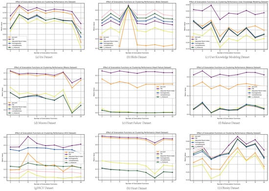
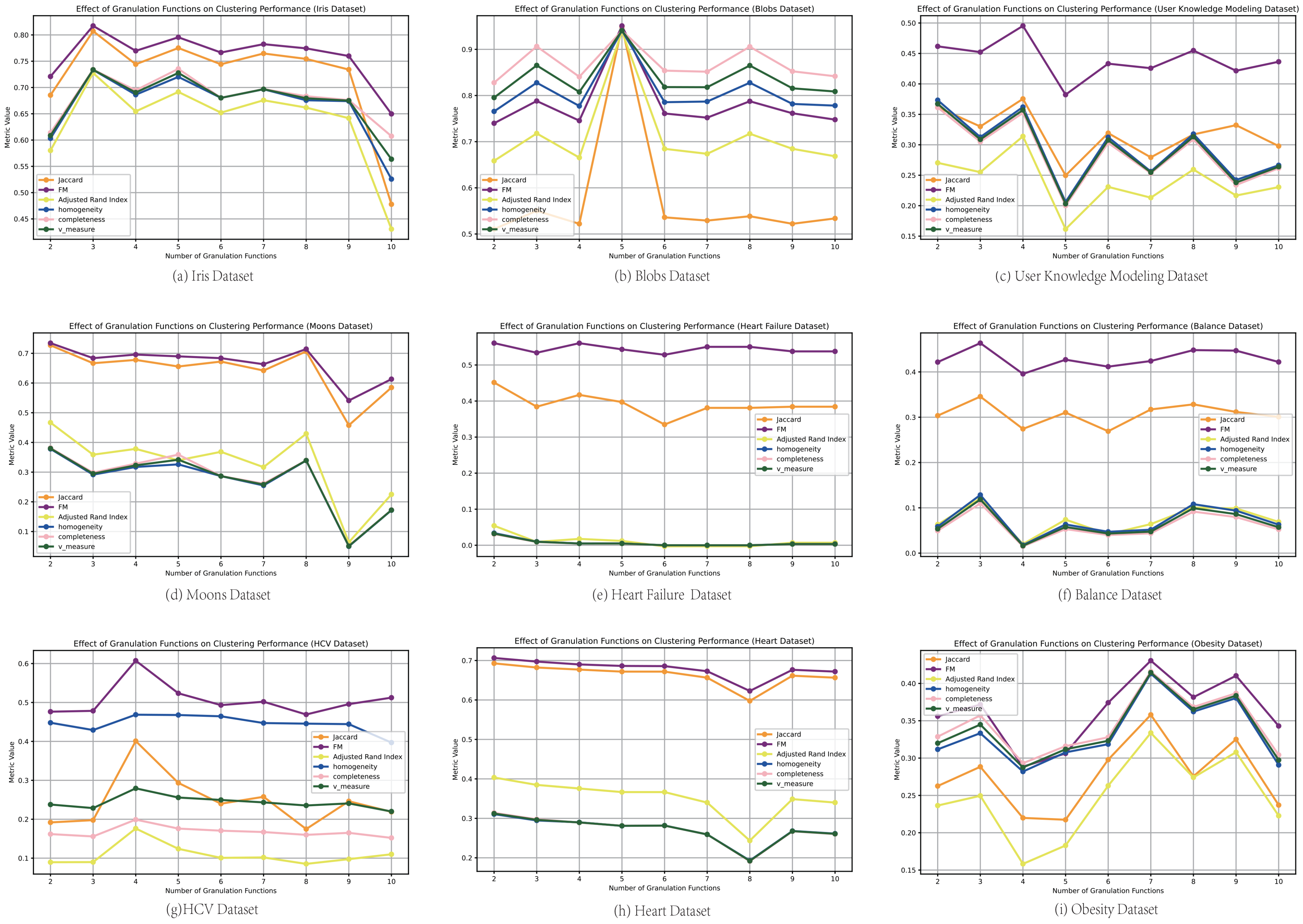
Metrics like purity (redundant with homogeneity), Silhouette Score (not directly reflecting label alignment), Calinski-Harabasz (CH), and DBI were excluded to ensure an efficient and non-redundant evaluation. The results across different granulation function counts for each dataset are shown in Figure 2.

Figure 2. Effect of the number of granulation functions.

From Figure 2a, on the Iris dataset, the performance differences between the counts of the granulation functions are small, with all metrics peaking when the function count is three. Scores decline at four, rebound at five, and drop steadily after seven. Figure 2b shows that on the Blobs dataset, increasing the count from two to three significantly improves five metrics, reaching a peak at five (all above 90%), but no further improvement is observed thereafter. For the User Knowledge Modeling dataset (Figure 2c), the optimal results are for four functions. Performance declines by ∼10% at five, slightly recovers at six, and then drops again. On the Moons dataset (Figure 2d), the highest scores are obtained with two functions, and no subsequent configuration surpasses this peak.

On the Heart Failure dataset (Figure 2e), Jaccard and FM peak at two functions, while the other four metrics remain below 10%. On the Balance dataset (Figure 2f), Jaccard and FM peak at three, dip by ∼5% at four, and then fluctuate slightly without surpassing the peak. For HCV (Figure 2g), Jaccard increases slightly from two to three, peaks with a 20% jump at four, and drops significantly after five; FM follows a similar pattern. Homogeneity decreases from two to three, slightly rebounds at four, and then declines again. The other three metrics also peak at four. On the Heart dataset (Figure 2h), most metrics peak at two functions and steadily decline, hitting a low at eight. The Obesity dataset (Figure 2i) shows a consistent trend across all six metrics, peaking at seven functions after initial fluctuation.

Comprehensive analysis reveals that FGK-means performs best when the number of granulation functions matches the actual number of classes in the dataset. For instance, Iris and Balance each have three classes, Blobs has five, Moons has two, Heart Failure has two, User Knowledge Modeling and HCV have four, Breast Tissue has six, and Obesity has seven. Experimental results indicate that aligning the number of granulation functions with the number of classes generally yields optimal clustering results. This offers valuable practical guidance: when performing data granulation, it is recommended to set the number of granulation functions equal to the dataset’s class count to achieve better clustering performance.

7.3. Comparison of Distance Metrics

In clustering algorithms, the choice of distance metric is crucial for determining sample similarity and significantly influences clustering outcomes. To systematically evaluate how different distance metrics affect FGK-means performance, a rigorous experimental framework was designed, testing three representative metrics: Euclidean distance, Manhattan distance, and cosine distance. A multi-dimensional evaluation system was constructed using three core metrics:

• Purity: Directly quantifies the alignment between clustering results and true labels, offering a straightforward measure of classification accuracy.
• Jaccard Index: Assesses the quality of cluster boundaries via sample pair matching accuracy and is more robust than ARI under class imbalance.
• Davies–Bouldin Index (DBI): An unsupervised metric reflecting intra-cluster compactness and inter-cluster separability; its $O\left(kn\right)$ time complexity makes it well-suited for large-scale datasets.

This evaluation system combines supervised metrics (purity and Jaccard) and an unsupervised metric (DBI), avoiding the redundancy of FM and ARI, while addressing the limitations of single-perspective metrics. These three metrics provide a comprehensive evaluation along orthogonal dimensions: label alignment, sample match accuracy, and structural rationality of clusters—meeting both effectiveness and efficiency requirements of the distance comparison experiment.

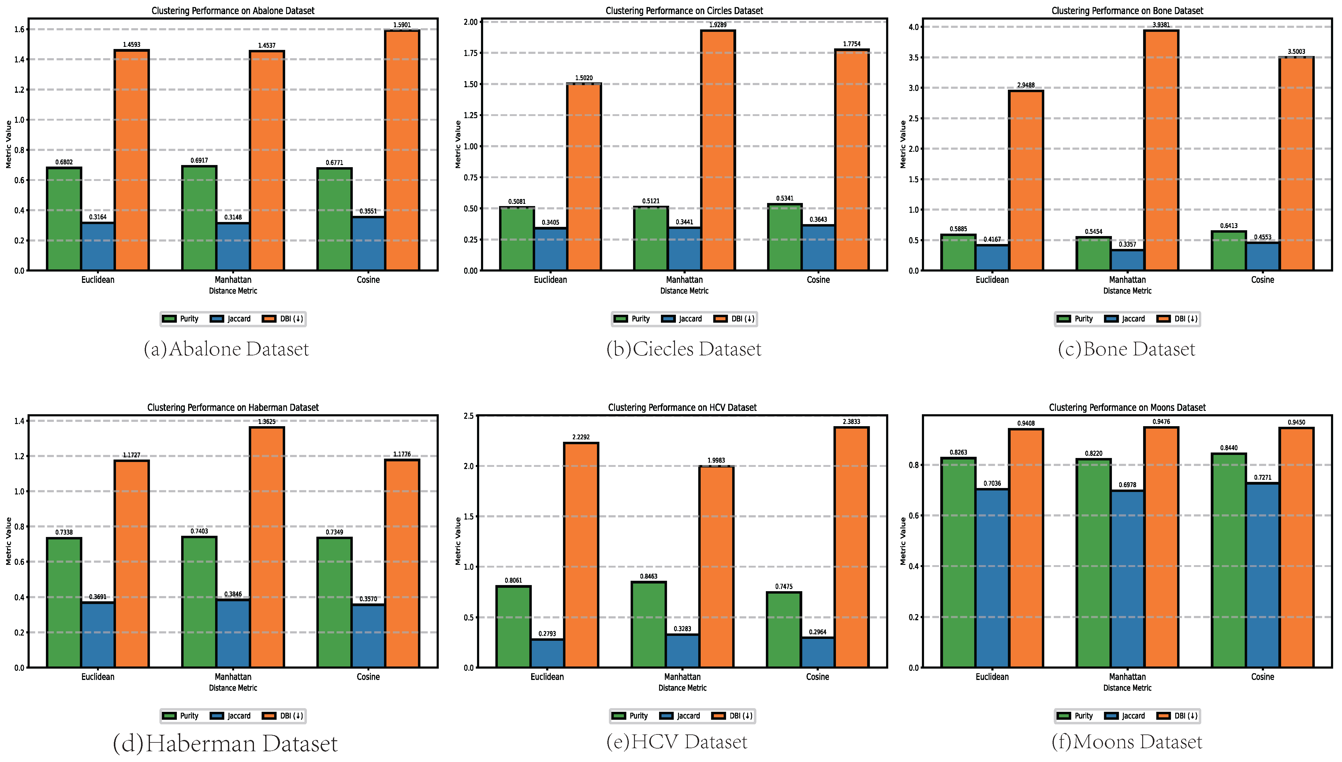
The experimental results are shown in Figure 3, highlighting performance differences across datasets when using different distance metrics.

Figure 3. Metric comparison results on various datasets. Note: The downward arrow (↓) indicates that a lower DBI value represents better performance.

In Figure 3a (Abalone dataset), the three distance metrics exhibit differentiated performance: Manhattan distance achieves the best purity, outperforming Euclidean and cosine distances by 1.15% and 1.46%, respectively. However, in terms of Jaccard, the cosine distance clearly surpasses the other two. Regarding the DBI index, Manhattan distance performs best. In Figure 3b (Circles dataset), cosine distance outperforms both Euclidean and Manhattan distances in both purity and Jaccard metrics, demonstrating excellent adaptability to non-convex data structures. Although its DBI is slightly higher than that of Manhattan distance, the difference is minimal. Results on the Bone dataset (Figure 3c) show that cosine distance improves purity by 5.28% over Euclidean distance and 9.59% over Manhattan distance. It also achieves the best Jaccard score. For DBI, Euclidean performs best, with cosine being slightly weaker. In Figure 3d (Haberman dataset), Manhattan distance achieves the best results in both purity and Jaccard among the three metrics. On the HCV dataset (Figure 3e), Manhattan distance shows a clear advantage in both purity and Jaccard, and although its DBI score is not the best, its overall performance is superior to the others. In Figure 3f (Moons dataset), cosine distance surpasses both Euclidean and Manhattan distances in purity and Jaccard, and its DBI score is only 0.44% lower than that of the best-performing Euclidean distance.

Based on the dataset characteristics and experimental results in Figure 3, the applicable scenarios for each distance metric can be summarized as follows:

1.

Manhattan Distance: Performs better on datasets with noise, outliers, and fuzzy class boundaries (e.g., Haberman and HCV). It shows improved purity over Euclidean and cosine distances, and its DBI value remains stable, indicating strong robustness to feature scale differences and outliers.

2.

Cosine Distance: More advantageous for datasets with directional sensitivity and non-convex structures (e.g., Circles and Moons). It significantly outperforms Euclidean and Manhattan in Jaccard, particularly excelling in capturing geometric patterns like ring and crescent shapes.

7.4. Comparison of Algorithm Variants

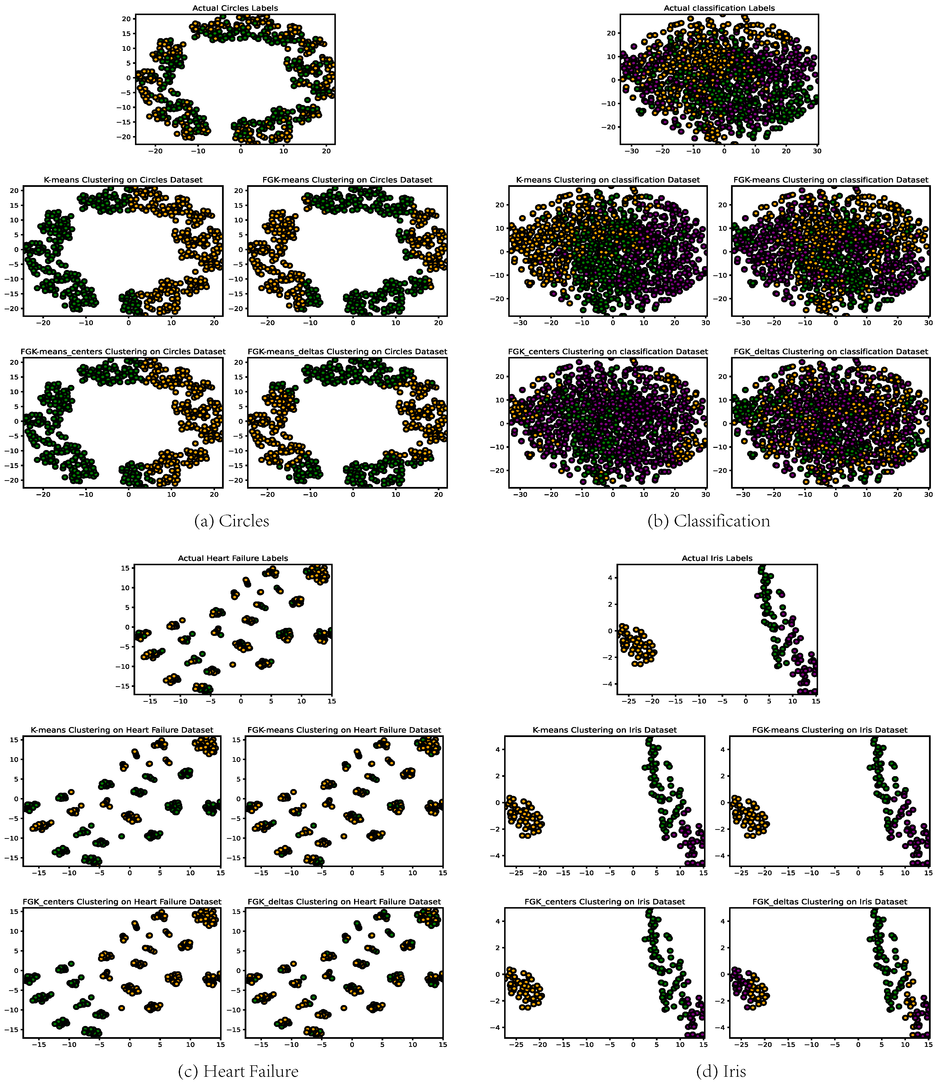
To further explore how different initialization strategies affect FGK-means clustering performance, three distinct initialization variants were designed for comparative analysis. Using t-SNE for dimensionality reduction, clustering results and actual distributions are visualized in Figure 4, enabling direct comparison. The three variants are as follows:

Figure 4. Comparison of FGK-means initialization variants.

1.

FGK-means All Random: Gaussian centers are randomly chosen in the range $(\mu -\sigma ,\mu +\sigma )$, with the standard deviation randomly in $(0.5\sigma ,1.5\sigma )$.

2.

FGK-means Centers Random: Centers are randomly selected in $(\mu -\sigma ,\mu +\sigma )$, while the standard deviation is fixed to $\sigma$.

3.

FGK-means Deltas Random: The center is fixed at $\mu$, and the standard deviation is randomly in $(0.5\sigma ,1.5\sigma )$.

From Figure 4, it is evident that FGK-means all random demonstrates the best adaptability. Its clustering boundaries align closely with true distributions, especially in regions of overlap or fuzzy boundaries. By contrast, centers random maintains center variability, but a fixed standard deviation causes coverage mismatch. Deltas random suffers from clustering bias due to a fixed center, especially on non-uniform data.

Compared with traditional K-means, FGK-means all random has notable advantages: while K-means assumes fixed spherical clusters and hard assignments (resulting in linear boundaries), FGK-means all random leverages Gaussian modeling and dual-random initialization to avoid local optima and adapt cluster shape/size dynamically.

Experiments show that proper initialization is crucial, and FGK-means all random ensures both flexibility and accuracy.

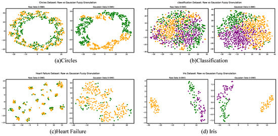
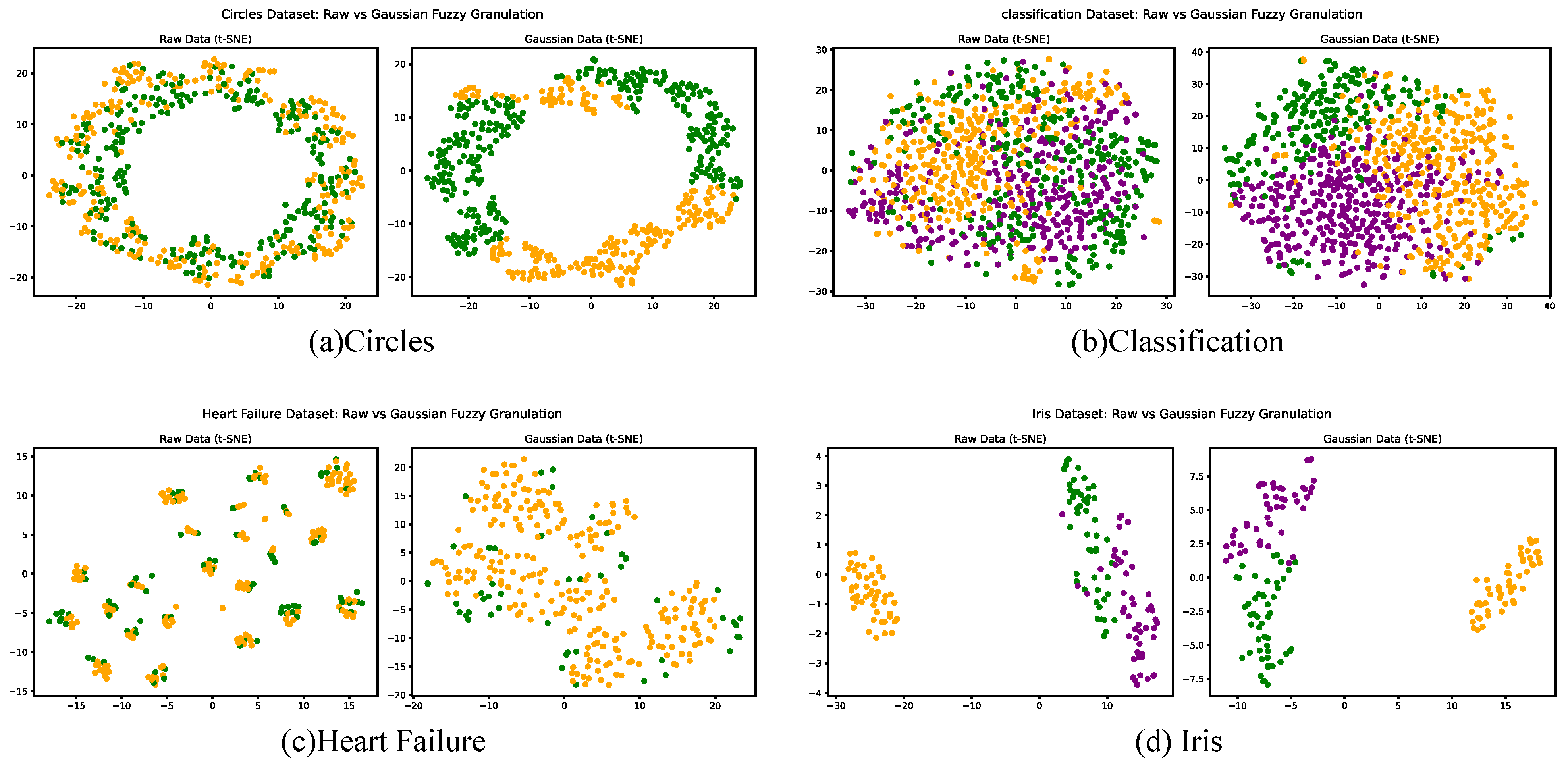
In order to show this mechanism intuitively, Figure 5 directly compares the original two-dimensional data distribution with the corresponding representation after Gaussian fuzzy processing. The left figure shows the original input, while the right figure shows the Gaussian fuzzy representation projected to two-dimensional space. The visualization highlights how the Gaussian membership mapping smooths local irregularities and extends overlapping manifolds into structures that are easier to separate, thus promoting the adaptive clustering behavior that FGK-means can observe. In short, the diagram visually explains why FGK-means can achieve better boundary alignment and robustness than the baseline method.

Figure 5. Comparison of the original data and Gaussian fuzzy.

7.5. Parameter Sensitivity

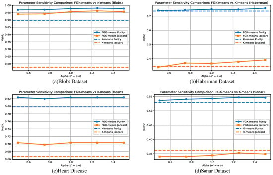
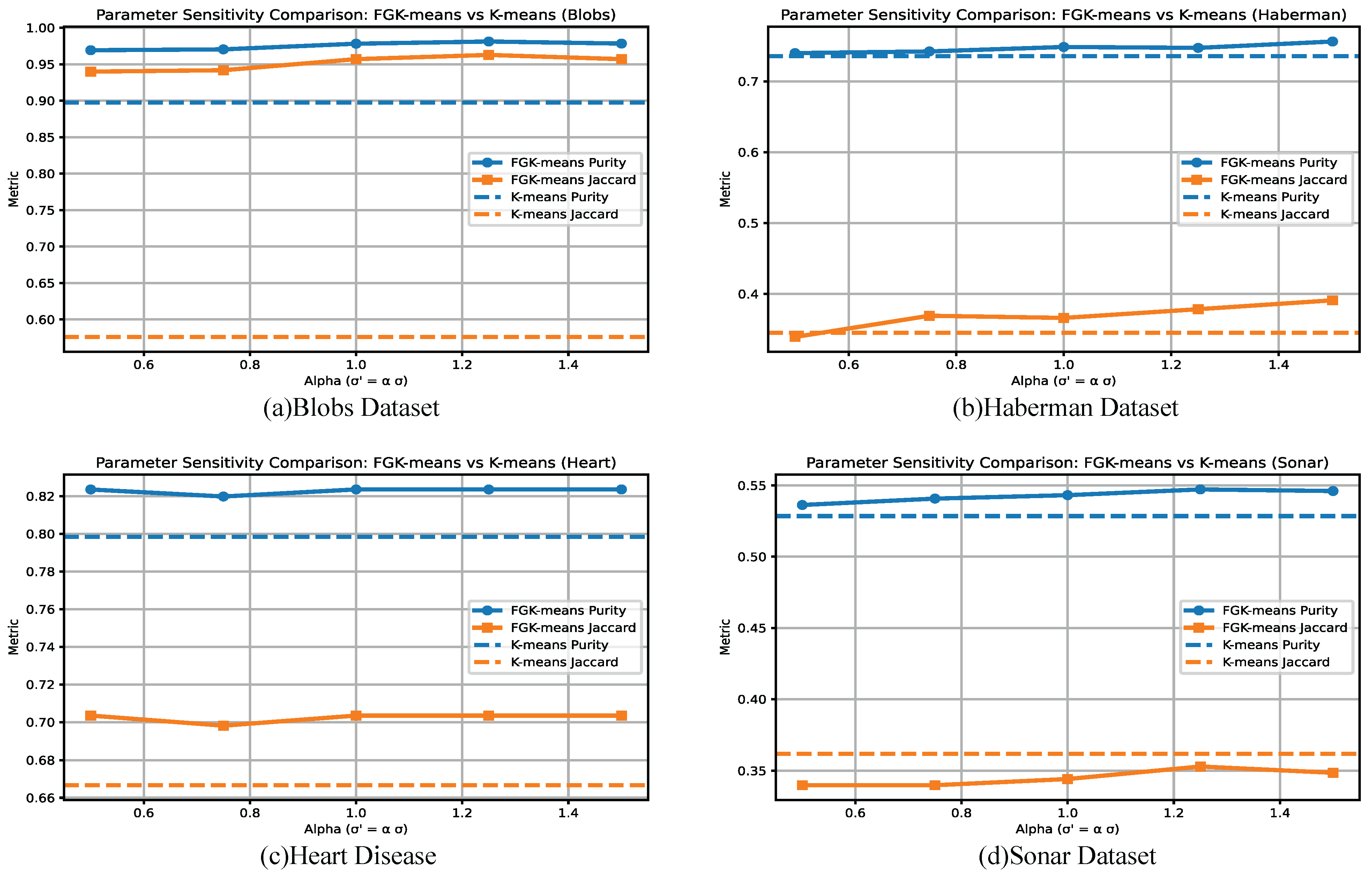
To further study the robustness of the FGK-means algorithm to the Gaussian membership parameters, we scaled the standard deviation $\sigma$ by the multiplication factor $\alpha \in 0.50,0.75,1.00,1.25,1.50$ to conduct a sensitivity analysis. For each $\alpha$ value, we reconstruct the Gauss-based fuzzy granules while keeping all other algorithm components unchanged. Cluster performance is evaluated using purity and the Jaccard index. Figure 6 shows the results of four representative datasets (Blobs, Haberman, Heart, and Sonar).

Figure 6. Comparison of the parameter sensitivity.

The Blobs dataset further enhances this robustness. Although the dataset contains multiple well-separated clusters, the FGK-means algorithm consistently performs well, with purity ranging from 0.967 to 0.981 and the Jaccard coefficient ranging from 0.936 to 0.963. The smaller fluctuation range (<2%) confirms that the Gaussian fuzzing mechanism is still stable in the convex cluster structure of the rule. On the Haberman dataset, the FGK-means algorithm also shows smooth, monotonous behavior. As $\alpha$ increases, the purity increases slightly from 0.740 to 0.756, while the Jaccard coefficient increases from 0.339 to 0.391. This gradual trend does not show any sudden decline in performance, highlighting the robustness of the granulation process in low-dimensional and category-unbalanced medical scenarios. On the Heart dataset, the fluctuation in purity and the Jaccard index is less than 1%, and the purity only varies between 0.819 and 0.824 under different $\alpha$ values. This near-flat performance curve shows that the algorithm’s sensitivity to $\sigma$ is extremely low, indicating that FGK-means can maintain stable granular representation even in noisy medical data. The Sonar dataset, which is famous for its high dimensionality and significant noise, also shows stable performance. The purity only fluctuates between 0.539 and 0.567, while the Jaccard coefficient remains between 0.348 and 0.353 throughout the $\alpha$ range. The observed small changes show that the FGK-means algorithm can maintain consistent performance even under challenging high-dimensional conditions.

On all four datasets, the fluctuations in purity and Jaccard coefficients remained between 1% and 3%, and no datasets showed instability or divergence at different $\sigma$ scales. These results together show that the granulation mechanism based on the Gaussian distribution is inherently robust. The FGK-means algorithm does not rely on fine-tuning of $\sigma$, which is an advantage for practical applications where parameter selection is usually difficult.

7.6. Comparison with Related Algorithms

Based on the experimental findings, FGK-means all random is identified as the optimal variant. Combining the optimal granulation function count and distance metric per dataset, this method is benchmarked against 11 mainstream machine learning clustering algorithms (K-means, GMM, Spectral Clustering, Agglomerative, FCM, Mean Shift, Affinity Propagation, Birch, and DBSCAN) and two deep clustering algorithms (DEC and ClusterGAN), as well as a novel neighborhood granular fuzzy C-means clustering algorithm (NGFCM). Three core indicators are emphasized:

• Purity: Reflects intra-cluster consistency via dominant class proportion;
• Jaccard Index: Measures overlap between predicted and actual labels;
• Fowlkes–Mallows Index (FM): Balances precision and recall with symmetry.

For all comparative clustering algorithms, the key parameters are set according to the default values commonly used in the standard implementation. This ensures the fairness and repeatability of the experimental comparison.

The analysis based on the experimental results in Table 5 on the Blobs dataset shows that the FGK-means algorithm demonstrates significant advantages across multiple key metrics. Specifically, it achieves a purity score of 0.978777, which is a 5.88% improvement over K-means (0.924004), and it also outperforms other mainstream algorithms such as Spectral (0.936101), Agglomerative (0.972081), and DEC (0.978758). For the Jaccard index, FGK-means scores 0.958227, clearly better than K-means (0.687111) and higher than Spectral (0.874415) and Agglomerative (0.943766). Regarding the Fowlkes–Mallows index (FM), FGK-means achieves 0.958899, which is 13.75% higher than K-means (0.842966), showing overall superiority over other clustering algorithms, second only to DEC by a margin of 0.285%. Notably, in the Adjusted Rand Index (ARI), FGK-means (0.948674) significantly outperforms traditional K-means (0.792217) and surpasses algorithms like Spectral (0.846711) and FCM (0.900479), achieving a discriminative accuracy close to the current top-performing DEC algorithm (0.949029). For internal evaluation metrics, FGK-means also excels: its Davies–Bouldin Index (DBI) (0.445170) is 27.62% lower than that of K-means, and its V-Measure (0.942666) improves by 6.58%, confirming its advances in inter-cluster separability and cluster structure balance. Although FGK-means shows a slight disadvantage in Silhouette Score (0.679843) and the Calinski–Harabasz Index compared to K-means, the differences are minimal (4.86%), which does not affect the overall superiority and robustness of the proposed method.

Table 5. Comparison of clustering performance on Blob dataset.

Dataset	Purity	Jaccard	FM	Adjusted Rand Index	Homogeneity	Completeness	V-Measure	Silhouette Score	Davies-Bouldin Index
K-means	$0.924004\pm 0.002206$	$0.687111\pm 0.054609$	$0.842966\pm 0.009910$	$0.792217\pm 0.018072$	$0.859897\pm 0.005274$	$0.911263\pm 0.000800$	$0.884427\pm 0.002647$	$0.648336\pm 0.001023$	$0.614852\pm 0.023741$
FGK-means	$\mathbf{0}.\mathbf{978777}\pm \mathbf{0}.\mathbf{000002}$	$\mathbf{0}.\mathbf{958227}\pm \mathbf{0}.\mathbf{000009}$	$0.958899\pm 0.000010$	$0.948674\pm 0.000015$	$0.942634\pm 0.000035$	$0.942698\pm 0.000035$	$0.942666\pm 0.000035$	$0.679843\pm 0.000013$	$0.445170\pm 0.000012$
Spectral	$0.936101\pm 0.000001$	$0.874415\pm 0.000003$	$0.877308\pm 0.000005$	$0.846711\pm 0.000007$	$0.855292\pm 0.000011$	$0.856326\pm 0.000011$	$0.855809\pm 0.000011$	$0.624254\pm 0.000018$	$0.498905\pm 0.000031$
Agglomerative	$0.972081\pm 0.000071$	$0.943766\pm 0.000381$	$0.945988\pm 0.000307$	$0.932518\pm 0.000481$	$0.933537\pm 0.000170$	$0.934319\pm 0.000137$	$0.933928\pm 0.000153$	$0.679268\pm 0.000014$	$0.445036\pm 0.000007$
GMM	$0.851423\pm 0.006639$	$0.588152\pm 0.010603$	$0.777255\pm 0.007460$	$0.688330\pm 0.015799$	$0.747767\pm 0.013972$	$0.914346\pm 0.005626$	$0.821827\pm 0.010517$	$0.538376\pm 0.016300$	$0.859359\pm 0.124943$
Mean Shift	$0.734779\pm 0.013915$	$0.507474\pm 0.018677$	$0.774246\pm 0.003206$	$0.665771\pm 0.009131$	$0.704134\pm 0.009288$	$0.987457\pm 0.000011$	$0.819526\pm 0.003901$	$0.707313\pm 0.000385$	$0.426210\pm 0.005038$
Affinity Propagation	$0.864348\pm 0.000023$	$0.274639\pm 0.003012$	$0.547817\pm 0.001633$	$0.372489\pm 0.003841$	$0.582660\pm 0.002590$	$0.688947\pm 0.001675$	$0.630449\pm 0.001464$	$0.107355\pm 0.021242$	$1.342844\pm 0.089900$
Birch	$0.871897\pm 0.004865$	$0.665279\pm 0.042923$	$0.840695\pm 0.015010$	$0.777312\pm 0.044667$	$0.817714\pm 0.025099$	$0.986880\pm 0.004688$	$0.894368\pm 0.013995$	$\mathbf{0}.\mathbf{730506}\pm \mathbf{0}.\mathbf{000005}$	$\mathbf{0}.\mathbf{343081}\pm \mathbf{0}.\mathbf{003202}$
FCM	$0.950310\pm 0.002338$	$0.826688\pm 0.050902$	$0.900573\pm 0.009865$	$0.870009\pm 0.017989$	$0.900479\pm 0.005618$	$0.926593\pm 0.000901$	$0.912941\pm 0.002864$	$0.668197\pm 0.000646$	$0.514366\pm 0.015910$
DBSCAN	$0.750002\pm 0.000067$	$0.427552\pm 0.000015$	$0.741956\pm 0.000064$	$0.611329\pm 0.000421$	$0.651545\pm 0.000035$	$\mathbf{0}.\mathbf{988135}\pm \mathbf{0}.\mathbf{000080}$	$0.785293\pm 0.000061$	$0.606161\pm 0.012380$	$0.437054\pm 0.000428$
DEC	$0.978758\pm 0.000003$	$\mathbf{0}.\mathbf{958227}\pm \mathbf{0}.\mathbf{000009}$	$\mathbf{0}.\mathbf{959184}\pm \mathbf{0}.\mathbf{00000}$	$\mathbf{0}.\mathbf{949029}\pm \mathbf{0}.\mathbf{000013}$	$\mathbf{0}.\mathbf{945182}\pm \mathbf{0}.\mathbf{000015}$	$0.945281\pm 0.000016$	$\mathbf{0}.\mathbf{945232}\pm \mathbf{0}.\mathbf{000015}$	$0.679233\pm 0.000002$	$0.445341\pm 0.000002$
ClusterGAN	$0.959749\pm 0.000196$	$0.920860\pm 0.000701$	$0.922325\pm 0.000710$	$0.902984\pm 0.001108$	$0.904476\pm 0.000826$	$0.904894\pm 0.000825$	$0.904685\pm 0.000826$	$0.648361\pm 0.000607$	$0.474925\pm 0.000391$
NGFCM	$0.660113\pm 0.035650$	$0.375125\pm 0.075585$	$0.624375\pm 0.043278$	$0.433744\pm 0.080191$	$0.493135\pm 0.089613$	$0.829537\pm 0.052385$	$0.616328\pm 0.086874$	$0.473790\pm 0.220022$	$0.644714\pm 0.224199$

Note: Bold values indicate the best performance for each metric.

In the experiments on the Moons dataset (Table 6, a nonlinearly separable crescent-shaped distribution), FGK-means demonstrates unique adaptability to complex manifold structures through its Gaussian fuzzy granulation mechanism. Compared to traditional K-means, the algorithm shows significant improvements in external evaluation metrics: purity increases from 0.8374562 to 0.852167 (+1.75%), the Jaccard index from 0.720202 to 0.731190 (+1.52%), the FM index from 0.726572 to 0.739630, and the Adjusted Rand Index from 0.454138 to 0.474421 (+4.46%). In terms of semantic consistency, FGK-means also improves: homogeneity increases from 0.359645 to 0.392196 (+9.06%) and completeness from 0.359739 to 0.398508 (+10.77%), significantly outperforming Spectral (0.361309/0.361417) and FCM (0.374078/0.374165). These results indicate that the FGK-means algorithm effectively captures the topological characteristics of crescent structures through nonlinear mapping and that its fuzzy granulation strategy enhances the logical cohesion within clusters. Overall, FGK-means not only outperforms traditional K-means in key external evaluation metrics like purity, Jaccard, and FM, but also demonstrates better overall performance than several mainstream clustering algorithms such as Spectral and GMM.

Table 6. Comparison of clustering performance on the Moons dataset.

Dataset	Purity	Jaccard	FM	Adjusted Rand Index	Homogeneity	Completeness	V-Measure	Silhouette Score	Davies-Bouldin Index
K-means	$0.837456\pm 0.000022$	$0.720202\pm 0.000046$	$0.726572\pm 0.000039$	$0.454138\pm 0.000155$	$0.359645\pm 0.000119$	$0.359739\pm 0.000120$	$0.359692\pm 0.000120$	$0.490141\pm 0.000030$	$0.814178\pm 0.000086$
FGK-means	$0.852167\pm 0.000023$	$0.731190\pm 0.000227$	$0.739630\pm 0.000096$	$0.474421\pm 0.000767$	$0.392196\pm 0.000102$	$0.398508\pm 0.000223$	$0.395286\pm 0.000136$	$0.424767\pm 0.000072$	$0.924553\pm 0.001846$
Spectral	$0.838140\pm 0.000037$	$0.721201\pm 0.000079$	$0.727502\pm 0.000067$	$0.455982\pm 0.0002644$	$0.361309\pm 0.000206$	$0.361417\pm 0.000207$	$0.361363\pm 0.000206$	$0.490152\pm 0.000028$	$0.814087\pm 0.000079$
Agglomerative	$0.902742\pm 0.000324$	$\mathbf{0}.\mathbf{787686}\pm \mathbf{0}.\mathbf{002408}$	$0.796824\pm 0.001701$	$0.581415\pm 0.008685$	$0.553935\pm 0.003576$	$0.576673\pm 0.002304$	$0.565006\pm 0.002932$	$0.450376\pm 0.000178$	$0.850578\pm 0.000059$
GMM	$0.780143\pm 0.001053$	$0.471415\pm 0.028428$	$0.681921\pm 0.000458$	$0.126103\pm 0.037551$	$0.131838\pm 0.022460$	$0.214213\pm 0.009781$	$0.148335\pm 0.021743$	$----$	$----$
Mean Shift	$0.873736\pm 0.000009$	$0.736135\pm 0.000063$	$0.750304\pm 0.000030$	$0.483527\pm 0.000216$	$0.447377\pm 0.000086$	$0.471121\pm 0.000161$	$0.458931\pm 0.000114$	$0.433029\pm 0.000004$	$0.853828\pm 0.000024$
Affinity Propagation	$0.849215\pm 0.000136$	$0.268138\pm 0.003413$	$0.627497\pm 0.000032$	$0.050322\pm 0.000621$	$0.151196\pm 0.000199$	$0.202142\pm 0.000286$	$0.172937\pm 0.000225$	$----$	$----$
Birch	$0.889514\pm 0.000617$	$0.756715\pm 0.003498$	$0.770995\pm 0.002508$	$0.523224\pm 0.012541$	$0.506712\pm 0.007765$	$0.535039\pm 0.006024$	$0.520410\pm 0.006905$	$0.442723\pm 0.000170$	$0.850320\pm 0.000114$
FCM	$0.843444\pm 0.000040$	$0.729142\pm 0.000092$	$0.734794\pm 0.000077$	$0.470561\pm 0.000310$	$0.374078\pm 0.000237$	$0.374165\pm 0.000235$	$0.374122\pm 0.000236$	$\mathbf{0}.\mathbf{490291}\pm \mathbf{0}.\mathbf{000031}$	$0.814031\pm 0.000086$
DBSCAN	$\mathbf{0}.\mathbf{992753}\pm \mathbf{0}.\mathbf{000025}$	$0.658770\pm 0.321624$	$\mathbf{0}.\mathbf{985418}\pm \mathbf{0}.\mathbf{000099}$	$\mathbf{0}.\mathbf{970891}\pm \mathbf{0}.\mathbf{000396}$	$\mathbf{0}.\mathbf{944034}\pm \mathbf{0}.\mathbf{001265}$	$\mathbf{0}.\mathbf{944152}\pm \mathbf{0}.\mathbf{001259}$	$\mathbf{0}.\mathbf{944093}\pm \mathbf{0}.\mathbf{001262}$	$----$	$----$
DEC	$0.839288\pm 0.000036$	$0.722194\pm 0.000091$	$0.728614\pm 0.000074$	$0.457806\pm 0.000308$	$0.363762\pm 0.000216$	$0.364239\pm 0.000208$	$0.364000\pm 0.000212$	$0.400906\pm 0.000083$	$1.013570\pm 0.000400$
ClusterGAN	$0.834166\pm 0.000852$	$0.715974\pm 0.001820$	$0.723191\pm 0.001509$	$0.447368\pm 0.006000$	$0.354789\pm 0.004591$	$0.354923\pm 0.004606$	$0.354856\pm 0.004598$	$0.455933\pm 0.002610$	$\mathbf{0}.\mathbf{889312}\pm \mathbf{0}.\mathbf{014742}$
NGFCM	$0.843422\pm 0.005174$	$0.729142\pm 0.007825$	$0.734785\pm 0.007172$	$0.470561\pm 0.014377$	$0.374035\pm 0.012524$	$0.374103\pm 0.012467$	$0.374069\pm 0.012496$	$0.490109\pm 0.004688$	$0.814331\pm 0.007919$

Note: Bold values indicate the best performance for each metric.

Table 7, Table 8 and Table 9 present a comparative performance analysis of FGK-means, K-means, and 10 other clustering algorithms on 19 benchmark datasets (excluding Blobs and Moons). For the purity metric (Table 7), FGK-means achieves the best performance on the Heart, Climate, and Sonar datasets. Although not the best on the remaining datasets, it still shows significant improvements over traditional K-means. For instance, on the Iris dataset, FGK-means improves purity by 2.6444%, trailing only Birch, which outperforms it by around 1%; on datasets like Circles, HCV, User Knowledge Modeling, and Land Mines, FGK-means achieves absolute improvements of no less than 4%. Regarding the Jaccard index (Table 8), FGK-means delivers top performance on seven datasets, including Circles, Heart, and Bone. Similarly, in the Fowlkes–Mallows (FM) index evaluation (Table 9), FGK-means shows competitive advantages on the Iris, Heart, and Sonar datasets. It is worth noting that although FGK-means may not perform the best on every dataset, it consistently outperforms the baseline K-means algorithm in all test cases except for the Pima Indians dataset, where its FM metric is lower than that of K-means. It is particularly outstanding on nonlinearly separable datasets such as Circles, demonstrating excellent adaptability.

Table 7. Comparative performance of clustering algorithms in purity metric across diverse datasets.

Dataset	K-Means	FGK-Means	Spectral	Agglomerative	GMM	Mean Shift	Affinity Propagation	Birch	FCM	DBSCAN	DEC	ClusterGAN	NGFCM
Iris	$0.894156\pm$ $0.000041$	$0.923085\pm$ $0.033035$	$0.813020\pm$ $0.000027$	$0.803090\pm$ $0.007688$	$0.796580\pm$ $0.000003$	$0.871592\pm$ $0.000002$	$0.816378\pm$ $0.000002$	$\mathbf{0}.\mathbf{936506}\pm$ $\mathbf{0}.\mathbf{004865}$	$0.887425\pm$ $0.000010$	$0.750000\pm$ $0.000000$	$0.781745\pm$ $0.000090$	$0.789304\pm$ $0.000050$	$0.736098\pm$ $0.068501$
Circles	$0.508674\pm$ $0.000025$	$0.540564\pm$ $0.000015$	$0.508008\pm$ $0.000052$	$0.504846\pm$ $0.000021$	$0.505762\pm$ $0.000100$	$0.518103\pm$ $0.000032$	$0.586140\pm$ $0.005125$	$0.513042\pm$ $0.000020$	$0.510676\pm$ $0.000065$	$\mathbf{0}.\mathbf{736160}\pm$ $\mathbf{0}.\mathbf{001299}$	$0.508016\pm$ $0.000048$	$0.508668\pm$ $0.000009$	$0.510676\pm$ $0.006600$
HCV	$0.804494\pm$ $0.000146$	$0.850063\pm$ $0.000007$	$0.855899\pm$ $0.000010$	$0.869730\pm$ $0.003902$	$0.678245\pm$ $0.004151$	$0.839736\pm$ $0.010225$	$\mathbf{0}.\mathbf{870951}\pm$ $\mathbf{0}.\mathbf{004568}$	$0.785899\pm$ $0.000685$	$0.852629\pm$ $0.000182$	$0.837628\pm$ $0.004808$	$0.856279\pm$ $0.000012$	$0.866705\pm$ $0.000003$	$0.897023\pm$ $0.012144$
Heart Failure	$0.664089\pm$ $0.000145$	$0.693492\pm$ $0.000165$	$0.677783\pm$ $0.000035$	$0.681465\pm$ $0.000157$	$0.659147\pm$ $0.001000$	$0.679683\pm$ $0.000002$	$\mathbf{0}.\mathbf{700545}\pm$ $\mathbf{0}.\mathbf{001483}$	$0.678991\pm$ $0.000014$	$0.678714\pm$ $0.001899$	$0.673055\pm$ $0.000385$	$0.677482\pm$ $0.000009$	$0.678904\pm$ $0.000001$	$0.678714\pm$ $0.000069$
User Knowledge Modeling	$0.617285\pm$ $0.001230$	$0.681546\pm$ $0.000133$	$0.564732\pm$ $0.000013$	$0.565125\pm$ $0.000155$	$0.369775\pm$ $0.002345$	$0.320099\pm$ $0.000132$	$\mathbf{0}.\mathbf{728230}\pm$ $\mathbf{0}.\mathbf{000050}$	$0.576305\pm$ $0.007067$	$0.515991\pm$ $0.000004$	$0.320099\pm$ $0.000000$	$0.514134\pm$ $0.005100$	$0.577385\pm$ $0.003458$	$0.555721\pm$ $0.002983$
Obesity	$0.414142\pm$ $0.000024$	$0.466694\pm$ $0.000154$	$0.435242\pm$ $0.002759$	$0.439995\pm$ $0.000009$	$0.389691\pm$ $0.000174$	$\mathbf{0}.\mathbf{622734}\pm$ $\mathbf{0}.\mathbf{007544}$	$0.583302\pm$ $0.000052$	$0.411041\pm$ $0.000021$	$0.292950\pm$ $0.000000$	$0.360914\pm$ $0.044024$	$0.430502\pm$ $0.001532$	$0.421120\pm$ $0.000659$	$0.292950\pm$ $0.000000$
Land Mines	$0.386160\pm$ $0.000005$	$0.476167\pm$ $0.006857$	$0.391393\pm$ $0.000002$	$0.380687\pm$ $0.000087$	$0.620707\pm$ $0.001508$	$0.355022\pm$ $0.016104$	$0.488349\pm$ $0.006850$	$0.488349\pm$ $0.006850$	$0.381554\pm$ $0.008792$	$\mathbf{0}.\mathbf{694170}\pm$ $\mathbf{0}.\mathbf{005751}$	$0.259385\pm$ $0.000169$	$0.364512\pm$ $0.003525$	$0.262590\pm$ $0.014435$
Gausssian	$0.256442\pm$ $0.000332$	$0.296693\pm$ $0.000148$	$0.249432\pm$ $0.000269$	$0.331340\pm$ $0.005558$	$0.270394\pm$ $0.000087$	$\mathbf{0}.\mathbf{556278}\pm$ $\mathbf{0}.\mathbf{095201}$	$0.376969\pm$ $0.001475$	$0.255913\pm$ $0.000052$	$0.285973\pm$ $0.000909$	$0.333467\pm$ $0.053440$	$0.250101\pm$ $0.000515$	$0.274674\pm$ $0.000740$	$0.346703\pm$ $0.089729$
Haberman’s Survival	$0.735526\pm$ $0.000000$	$0.747400\pm$ $0.000004$	$0.736687\pm$ $0.000674$	$0.629842\pm$ $0.000129$	$0.668403\pm$ $0.000026$	$0.731173\pm$ $0.000760$	$\mathbf{0}.\mathbf{764277}\pm$ $\mathbf{0}.\mathbf{000177}$	$0.733940\pm$ $0.000007$	$0.736401\pm$ $0.000156$	$0.590001\pm$ $0.000067$	$0.734741\pm$ $0.000000$	$0.735308\pm$ $0.000000$	$0.736401\pm$ $0.000000$
Heart	$0.782343\pm$ $0.000287$	$\mathbf{0}.\mathbf{822884}\pm$ $\mathbf{0}.\mathbf{000101}$	$0.796750\pm$ $0.000004$	$0.613328\pm$ $0.011686$	$0.566390\pm$ $0.000006$	$0.610987\pm$ $0.009218$	$0.785171\pm$ $0.000077$	$0.761821\pm$ $0.003472$	$0.790934\pm$ $0.000011$	$0.573831\pm$ $0.000371$	$0.764459\pm$ $0.000285$	$0.738234\pm$ $0.004445$	$0.790934\pm$ $0.000000$
Absenteesim	$0.452024\pm$ $0.000492$	$0.484398\pm$ $0.000323$	$0.490401\pm$ $0.000258$	$\mathbf{0}.\mathbf{530093}\pm$ $\mathbf{0}.\mathbf{000965}$	$0.509636\pm$ $0.000489$	$0.472867\pm$ $0.027996$	$0.454914\pm$ $0.000001$	$0.440485\pm$ $0.000364$	$0.449825\pm$ $0.002315$	$0.281081\pm$ $0.000000$	$0.359956\pm$ $0.002796$	$0.397978\pm$ $0.002130$	$0.288334\pm$ $0.000000$
Abalone	$0.654167\pm$ $0.000534$	$0.711027\pm$ $0.000100$	$0.690250\pm$ $0.000081$	$0.701609\pm$ $0.003747$	$\mathbf{0}.\mathbf{729054}\pm$ $\mathbf{0}.\mathbf{000620}$	$0.644185\pm$ $0.000036$	$0.804095\pm$ $0.000294$	$0.660362\pm$ $0.000304$	$0.647268\pm$ $0.001881$	$0.656262\pm$ $0.000099$	$0.681991\pm$ $0.000050$	$0.663410\pm$ $0.000004$	$0.722448\pm$ $0.070004$
Balance	$0.641318\pm$ $0.000733$	$0.668510\pm$ $0.000396$	$0.606327\pm$ $0.003248$	$0.614568\pm$ $0.001189$	$0.591625\pm$ $0.004414$	$0.460800\pm$ $0.000854$	$\mathbf{0}.\mathbf{742616}\pm$ $\mathbf{0}.\mathbf{010985}$	$0.676510\pm$ $0.008256$	$0.607100\pm$ $0.005330$	$0.550790\pm$ $0.024294$	$0.545449\pm$ $0.013527$	$0.679449\pm$ $0.002125$	$0.640251\pm$ $0.017130$
Bone	$0.575814\pm$ $0.000685$	$0.643886\pm$ $0.000085$	$0.545004\pm$ $0.000000$	$0.549217\pm$ $0.000038$	$0.612866\pm$ $0.000893$	$0.545455\pm$ $0.000013$	$0.576007\pm$ $0.000351$	$0.548341\pm$ $0.000168$	$0.556246\pm$ $0.000165$	$\mathbf{0}.\mathbf{766681}\pm$ $\mathbf{0}.\mathbf{000205}$	$0.585870\pm$ $0.000371$	$0.593260\pm$ $0.004845$	$0.569101\pm$ $0.016609$
Climate	$0.915607\pm$ $0.000007$	$\mathbf{0}.\mathbf{922872}\pm$ $\mathbf{0}.\mathbf{000008}$	$0.915084\pm$ $0.000000$	$0.915687\pm$ $0.000065$	$0.914089\pm$ $0.000005$	$0.914815\pm$ $0.000000$	$0.921018\pm$ $0.000020$	$0.917426\pm$ $0.000034$	$0.914690\pm$ $0.000023$	$0.859457\pm$ $0.007911$	$0.914851\pm$ $0.000064$	$0.914954\pm$ $0.036400$	$0.914203\pm$ $0.001037$
Classification	$0.530963\pm$ $0.000894$	$0.563283\pm$ $0.000317$	$0.531533\pm$ $0.000539$	$0.459927\pm$ $0.002111$	$0.508070\pm$ $0.002829$	$0.446113\pm$ $0.036706$	$\mathbf{0}.\mathbf{601743}\pm$ $\mathbf{0}.\mathbf{007671}$	$0.523112\pm$ $0.002707$	$0.523905\pm$ $0.002805$	$0.374796\pm$ $0.004633$	$0.405372\pm$ $0.000008$	$0.413787\pm$ $0.000412$	$0.563478\pm$ $0.047540$
Sonar	$0.552188\pm$ $0.000064$	$\mathbf{0}.\mathbf{760796}\pm$ $\mathbf{0}.\mathbf{000007}$	$0.686361\pm$ $0.016800$	$0.531469\pm$ $0.000026$	$0.551287\pm$ $0.000160$	$0.640743\pm$ $0.007269$	$0.718102\pm$ $0.008851$	$0.547964\pm$ $0.000628$	$0.552009\pm$ $0.000000$	$0.633008\pm$ $0.007073$	$0.568312\pm$ $0.001805$	$0.616048\pm$ $0.002000$	$0.552009\pm$ $0.000000$
Pima Indians	$0.631778\pm$ $0.000000$	$\mathbf{0}.\mathbf{792963}\pm$ $\mathbf{0}.\mathbf{046644}$	$0.632885\pm$ $0.000682$	$0.626813\pm$ $0.070842$	$0.636509\pm$ $0.019724$	$0.665556\pm$ $0.049097$	$0.751146\pm$ $0.000000$	$0.631014\pm$ $0.004321$	$0.642716\pm$ $0.000519$	$0.672253\pm$ $0.109050$	$0.631682\pm$ $0.007181$	$0.648514\pm$ $0.002987$	$0.642716\pm$ $0.000519$
Hepatitis	$0.749892\pm$ $0.004076$	$0.881658\pm$ $0.015931$	$0.740539\pm$ $0.003588$	$0.750513\pm$ $0.000000$	$0.770316\pm$ $0.029221$	$0.678255\pm$ $0.002685$	$0.823842\pm$ $0.000000$	$0.725635\pm$ $0.000000$	$0.790223\pm$ $0.000000$	$\mathbf{0}.\mathbf{927928}\pm$ $\mathbf{0}.\mathbf{000000}$	$0.788597\pm$ $0.004590$	$0.792351\pm$ $0.001612$	$0.790223\pm$ $0.000000$

Note: Bold values indicate the best performance for each metric.

Table 8. Comparative performance of clustering algorithms in Jaccard metric across diverse datasets.

Dataset	K-Means	FGK-Means	Spectral	Agglomerative	GMM	Mean Shift	Affinity Propagation	Birch	FCM	DBSCAN	DEC	ClusterGAN	NGFCM
Iris	$0.796407\pm$ $0.000000$	$0.842809\pm$ $0.066117$	$0.679116\pm$ $0.000030$	$0.636905\pm$ $0.016608$	$0.642607\pm$ $0.000662$	$0.654423\pm$ $0.000028$	$0.100258\pm$ $0.000022$	$\mathbf{0}.\mathbf{834860}\pm$ $\mathbf{0}.\mathbf{042923}$	$0.789279\pm$ $0.000038$	$0.500000\pm$ $0.000000$	$0.636505\pm$ $0.000349$	$0.651420\pm$ $0.000109$	$0.492611\pm$ $0.010450$
Circles	$0.341092\pm$ $0.000021$	$\mathbf{0}.\mathbf{369868}\pm$ $\mathbf{0}.\mathbf{000011}$	$0.340503\pm$ $0.000042$	$0.337503\pm$ $0.000017$	$0.337521\pm$ $0.000053$	$0.219823\pm$ $0.000564$	$0.276095\pm$ $0.000080$	$0.344695\pm$ $0.000014$	$0.342909\pm$ $0.000053$	$0.343499\pm$ $0.000030$	$0.340502\pm$ $0.000039$	$0.341086\pm$ $0.000008$	$0.342909\pm$ $0.005943$
HCV	$0.253823\pm$ $0.000002$	$0.411354\pm$ $0.017327$	$0.207076\pm$ $0.000018$	$0.374344\pm$ $0.000087$	$0.472987\pm$ $0.007799$	$0.365657\pm$ $0.010225$	$\mathbf{0}.\mathbf{577523}\pm$ $\mathbf{0}.\mathbf{038026}$	$0.266804\pm$ $0.000131$	$0.208481\pm$ $0.004559$	$0.006597\pm$ $0.000077$	$0.207853\pm$ $0.002789$	$0.138188\pm$ $0.000003$	$0.364143\pm$ $0.001888$
Heart Failure	$0.422346\pm$ $0.001678$	$0.471073\pm$ $0.014467$	$0.362187\pm$ $0.001903$	$0.390698\pm$ $0.005603$	$\mathbf{0}.\mathbf{486946}\pm$ $\mathbf{0}.\mathbf{001378}$	$0.471773\pm$ $0.005330$	$0.465686\pm$ $0.001273$	$0.369486\pm$ $0.000042$	$0.350905\pm$ $0.000003$	$0.483871\pm$ $0.000019$	$0.354362\pm$ $0.000822$	$0.356125\pm$ $0.000236$	$0.350905\pm$ $0.001440$
User Knowledge Modeling	$0.347278\pm$ $0.000441$	$\mathbf{0}.\mathbf{406708}\pm$ $\mathbf{0}.\mathbf{000161}$	$0.298604\pm$ $0.000001$	$0.331669\pm$ $0.001786$	$0.198508\pm$ $0.000520$	$0.190547\pm$ $0.000572$	$0.073713\pm$ $0.000001$	$0.353896\pm$ $0.004748$	$0.284806\pm$ $0.000006$	$0.190547\pm$ $0.000000$	$0.305187\pm$ $0.003320$	$0.344893\pm$ $0.001621$	$0.335915\pm$ $0.002090$
Obesity	$0.330598\pm$ $0.001182$	$0.370284\pm$ $0.000000$	$0.355611\pm$ $0.000113$	$0.305725\pm$ $0.000232$	$0.268025\pm$ $0.000011$	$0.196276\pm$ $0.000054$	$0.166970\pm$ $0.027709$	$0.354432\pm$ $0.000000$	$0.271476\pm$ $0.000000$	$0.188156\pm$ $0.000019$	$\mathbf{0}.\mathbf{371288}\pm$ $\mathbf{0}.\mathbf{000459}$	$0.337282\pm$ $0.000011$	$0.171476\pm$ $0.000000$
Land Mines	$0.183888\pm$ $0.001817$	$\mathbf{0}.\mathbf{246055}\pm$ $\mathbf{0}.\mathbf{000002}$	$0.183895\pm$ $0.000013$	$0.161000\pm$ $0.000268$	$0.215100\pm$ $0.000669$	$\mathbf{0}.\mathbf{165881}\pm$ $\mathbf{0}.\mathbf{001770}$	$0.038948\pm$ $0.000021$	$0.171627\pm$ $0.000087$	$0.183888\pm$ $0.000117$	$0.126667\pm$ $0.000000$	$0.141898\pm$ $0.000011$	$0.200220\pm$ $0.001642$	$0.133603\pm$ $0.003236$
Gausssian	$0.142077\pm$ $0.000154$	$\mathbf{0}.\mathbf{166878}\pm$ $\mathbf{0}.\mathbf{000030}$	$0.138600\pm$ $0.000137$	$0.154830\pm$ $0.000167$	$0.152118\pm$ $0.000076$	$0.115250\pm$ $0.000014$	$0.107503\pm$ $0.000138$	$0.138122\pm$ $0.000058$	$0.135527\pm$ $0.000041$	$0.074074\pm$ $0.004115$	$0.137695\pm$ $0.000066$	$0.154903\pm$ $0.000293$	$0.132085\pm$ $0.003200$
Haberman’s Survival	$0.349014\pm$ $0.000012$	$0.395342\pm$ $0.000429$	$0.350993\pm$ $0.000078$	$0.582761\pm$ $0.000006$	$\mathbf{0}.\mathbf{599306}\pm$ $\mathbf{0}.\mathbf{000006}$	$0.449668\pm$ $0.011616$	$0.479127\pm$ $0.001953$	$0.364783\pm$ $0.001543$	$0.356984\pm$ $0.000791$	$0.011023\pm$ $0.000015$	$0.359039\pm$ $0.000093$	$0.346086\pm$ $0.000091$	$0.356984\pm$ $0.000000$
Heart	$0.641649\pm$ $0.000765$	$\mathbf{0}.\mathbf{701752}\pm$ $\mathbf{0}.\mathbf{000182}$	$0.664957\pm$ $0.000009$	$0.439199\pm$ $0.006753$	$0.361346\pm$ $0.000004$	$0.391827\pm$ $0.000156$	$0.384615\pm$ $0.000343$	$0.607143\pm$ $0.000169$	$0.656442\pm$ $0.008188$	$0.243744\pm$ $0.027518$	$0.617067\pm$ $0.000733$	$0.586519\pm$ $0.006796$	$0.656442\pm$ $0.000000$
Absenteesim	$0.095222\pm$ $0.000011$	$0.116142\pm$ $0.000005$	$0.091188\pm$ $0.000017$	$\mathbf{0}.\mathbf{118682}\pm$ $\mathbf{0}.\mathbf{000020}$	$0.117849\pm$ $0.000041$	$0.013383\pm$ $0.000225$	$0.042254\pm$ $0.000004$	$0.100164\pm$ $0.000107$	$0.021808\pm$ $0.001383$	$0.000676\pm$ $0.000000$	$0.035953\pm$ $0.000034$	$0.058153\pm$ $0.000400$	$0.058971\pm$ $0.008170$
Abalone	$0.318240\pm$ $0.000004$	$0.321341\pm$ $0.002595$	$0.302514\pm$ $0.000155$	$0.393910\pm$ $0.000548$	$0.360867\pm$ $0.000108$	$0.305371\pm$ $0.000013$	$\mathbf{0}.\mathbf{452975}\pm$ $\mathbf{0}.\mathbf{000082}$	$0.364727\pm$ $0.007312$	$0.314039\pm$ $0.003661$	$0.119689\pm$ $0.000254$	$0.299299\pm$ $0.000134$	$0.312090\pm$ $0.000112$	$0.410449\pm$ $0.072767$
Balance	$0.339343\pm$ $0.000115$	$0.359143\pm$ $0.001904$	$0.301608\pm$ $0.002627$	$0.317029\pm$ $0.004355$	$0.293872\pm$ $0.002374$	$0.299376\pm$ $0.000000$	$0.261500\pm$ $0.000280$	$0.356210\pm$ $0.001963$	$0.290903\pm$ $0.004390$	$0.199584\pm$ $0.029875$	$0.268068\pm$ $0.009109$	$\mathbf{0}.\mathbf{380720}\pm$ $\mathbf{0}.\mathbf{002166}$	$0.324406\pm$ $0.018331$
Bone	$0.408050\pm$ $0.000573$	$\mathbf{0}.\mathbf{457454}\pm$ $\mathbf{0}.\mathbf{000674}$	$0.363321\pm$ $0.000033$	$0.345324\pm$ $0.000000$	$0.446314\pm$ $0.000952$	$0.375000\pm$ $0.000143$	$0.316901\pm$ $0.006351$	$0.385223\pm$ $0.000080$	$0.383633\pm$ $0.000322$	$0.009158\pm$ $0.000252$	$0.416842\pm$ $0.000371$	$0.412967\pm$ $0.007403$	$0.390954\pm$ $0.029157$
Climate	$0.367260\pm$ $0.000354$	$0.418266\pm$ $0.000680$	$0.348919\pm$ $0.000086$	$0.491001\pm$ $0.003047$	$0.373063\pm$ $0.001598$	$\mathbf{0}.\mathbf{843003}\pm$ $\mathbf{0}.\mathbf{000000}$	$0.043478\pm$ $0.000012$	$0.379569\pm$ $0.000538$	$0.358082\pm$ $0.000330$	$0.792933\pm$ $0.002416$	$0.343925\pm$ $0.000170$	$0.341666\pm$ $0.000104$	$0.365340\pm$ $0.027711$
Classification	$0.363419\pm$ $0.000894$	$\mathbf{0}.\mathbf{393000}\pm$ $\mathbf{0}.\mathbf{001889}$	$0.361085\pm$ $0.000477$	$0.276591\pm$ $0.001523$	$0.339996\pm$ $0.002685$	$0.202165\pm$ $0.000001$	$0.189537\pm$ $0.000008$	$0.332868\pm$ $0.000255$	$0.334594\pm$ $0.003162$	$0.134375\pm$ $0.013543$	$0.249229\pm$ $0.000019$	$0.251364\pm$ $0.000113$	$0.330711\pm$ $0.040504$
Sonar	$0.378492\pm$ $0.000049$	$0.354752\pm$ $0.005068$	$0.347151\pm$ $0.000162$	$0.358865\pm$ $0.000007$	$0.378714\pm$ $0.000504$	$0.351482\pm$ $0.000026$	$0.300007\pm$ $0.001621$	$0.348572\pm$ $0.000077$	$0.380000\pm$ $0.000000$	$0.350099\pm$ $0.000202$	$0.393295\pm$ $0.001944$	$\mathbf{0}.\mathbf{446865}\pm$ $\mathbf{0}.\mathbf{002128}$	$0.380000\pm$ $0.000000$
Pima Indians	$0.501466\pm$ $0.000000$	$0.485016\pm$ $0.001354$	$0.503428\pm$ $0.001836$	$0.484061\pm$ $0.002030$	$0.397207\pm$ $0.060400$	$0.476588\pm$ $0.014241$	$0.474088\pm$ $0.000000$	$\mathbf{0}.\mathbf{504903}\pm$ $\mathbf{0}.\mathbf{002504}$	$0.500489\pm$ $0.000691$	$0.001087\pm$ $0.000814$	$0.488876\pm$ $0.005828$	$0.428454\pm$ $0.037016$	$0.500489\pm$ $0.000691$
Hepatitis	$0.606333\pm$ $0.013592$	$0.563782\pm$ $0.073741$	$0.634487\pm$ $0.008096$	$0.712707\pm$ $0.000000$	$0.604236\pm$ $0.160177$	$0.565979\pm$ $0.022598$	$0.569670\pm$ $0.045956$	$0.640212\pm$ $0.000000$	$0.512195\pm$ $0.000000$	$\mathbf{0}.\mathbf{727071}\pm$ $\mathbf{0}.\mathbf{000000}$	$0.465687\pm$ $0.040127$	$0.463328\pm$ $0.039473$	$0.512195\pm$ $0.000000$

Note: Bold values indicate the best performance for each metric.

Table 9. Comparative performance of clustering algorithms in FM metric across diverse datasets.

Dataset	K-Means	FGK-Means	Spectral	Agglomerative	GMM	Mean Shift	Affinity Propagation	Birch	FCM	DBSCAN	DEC	ClusterGAN	NGFCM
Iris	$0.810180\pm$ $0.000003$	$0.853192\pm$ $0.058751$	$0.714887\pm$ $0.000017$	$0.689603\pm$ $0.010231$	$0.713288\pm$ $0.000004$	$0.747012\pm$ $0.000001$	$0.513731\pm$ $0.000010$	$0.883444\pm$ $0.015010$	$0.803737\pm$ $0.000023$	$0.771454\pm$ $0.001206$	$0.666682\pm$ $0.000712$	$0.706082\pm$ $0.000026$	$0.712688\pm$ $0.043823$
Circles	$0.498404\pm$ $0.000085$	$0.504505\pm$ $0.000014$	$0.498558\pm$ $0.000228$	$0.514613\pm$ $0.000137$	$0.587618\pm$ $0.010835$	$0.483292\pm$ $0.002605$	$0.614781\pm$ $0.000275$	$0.504469\pm$ $0.000023$	$0.498681\pm$ $0.000107$	$\mathbf{0}.\mathbf{690852}\pm$ $\mathbf{0}.\mathbf{000118}$	$0.498620\pm$ $0.000383$	$0.498194\pm$ $0.001668$	$0.498681\pm$ $0.000002$
HCV	$0.492158\pm$ $0.000729$	$0.682256\pm$ $0.004960$	$0.461589\pm$ $0.000005$	$0.634893\pm$ $0.000043$	$\mathbf{0}.\mathbf{702775}\pm$ $\mathbf{0}.\mathbf{005110}$	$0.622258\pm$ $0.000020$	$0.727514\pm$ $0.029696$	$0.547182\pm$ $0.000237$	$0.429666\pm$ $0.001272$	$0.624269\pm$ $0.000002$	$0.431094\pm$ $0.000722$	$0.391590\pm$ $0.000003$	$0.596194\pm$ $0.019107$
Heart Failure	$0.572379\pm$ $0.000930$	$0.592886\pm$ $0.006258$	$0.530519\pm$ $0.000305$	$0.563830\pm$ $0.000079$	$0.638680\pm$ $0.000380$	$0.686773\pm$ $0.012010$	$0.702175\pm$ $0.000027$	$0.536488\pm$ $0.000045$	$0.528845\pm$ $0.000001$	$\mathbf{0}.\mathbf{720767}\pm$ $\mathbf{0}.\mathbf{000000}$	$0.532388\pm$ $0.000049$	$0.529807\pm$ $0.000003$	$0.528845\pm$ $0.000137$
User Knowledge Modeling	$0.422488\pm$ $0.001230$	$0.519813\pm$ $0.000464$	$0.360838\pm$ $0.000013$	$0.432428\pm$ $0.000155$	$0.304017\pm$ $0.000285$	$\mathbf{0}.\mathbf{521302}\pm$ $\mathbf{0}.\mathbf{000001}$	$0.464403\pm$ $0.000002$	$0.431626\pm$ $0.005616$	$0.407756\pm$ $0.000010$	$0.521302\pm$ $0.000491$	$0.387192\pm$ $0.003273$	$0.437475\pm$ $0.001733$	$0.000000\pm$ $0.000000$
Obesity	$0.351330\pm$ $0.002411$	$0.463098\pm$ $0.000121$	$0.439707\pm$ $0.000036$	$0.426383\pm$ $0.001262$	$0.445204\pm$ $0.000002$	$0.470275\pm$ $0.000176$	$0.473174\pm$ $0.000001$	$0.441028\pm$ $0.000003$	$0.452313\pm$ $0.000000$	$\mathbf{0}.\mathbf{478435}\pm$ $\mathbf{0}.\mathbf{000000}$	$0.453950\pm$ $0.000261$	$0.417358\pm$ $0.000485$	$0.352313\pm$ $0.000000$
Land Mines	$0.246610\pm$ $0.0000717$	$0.295383\pm$ $0.000763$	$0.248231\pm$ $0.000029$	$0.227293\pm$ $0.000136$	$0.394580\pm$ $0.000130$	$0.419519\pm$ $0.000513$	$0.367632\pm$ $0.000009$	$0.261460\pm$ $0.000837$	$0.245821\pm$ $0.001472$	$\mathbf{0}.\mathbf{437636}\pm$ $\mathbf{0}.\mathbf{000001}$	$0.199883\pm$ $0.000003$	$0.269470\pm$ $0.002059$	$0.227653\pm$ $0.015892$
Gausssian	$0.200778\pm$ $0.000014$	$0.220233\pm$ $0.000086$	$0.200481\pm$ $0.000011$	$0.233726\pm$ $0.000250$	$0.211959\pm$ $0.000017$	$0.441089\pm$ $0.000015$	$0.397023\pm$ $0.000086$	$0.211476\pm$ $0.000013$	$0.272871\pm$ $0.001538$	$\mathbf{0}.\mathbf{444833}\pm$ $\mathbf{0}.\mathbf{000001}$	$0.200388\pm$ $0.000027$	$0.210767\pm$ $0.000144$	$0.274993\pm$ $0.031398$
Haberman’s Survival	$0.550611\pm$ $0.000000$	$0.575522\pm$ $0.000015$	$0.551024\pm$ $0.000006$	$0.759753\pm$ $0.000004$	$0.740366\pm$ $0.000004$	$0.643457\pm$ $0.012745$	$0.689747\pm$ $0.001643$	$0.558850\pm$ $0.000227$	$0.551386\pm$ $0.000065$	$\mathbf{0}.\mathbf{759899}\pm$ $\mathbf{0}.\mathbf{000046}$	$0.551903\pm$ $0.000000$	$0.550537\pm$ $0.000002$	$0.551386\pm$ $0.000000$
Heart	$0.663484\pm$ $0.000250$	$\mathbf{0}.\mathbf{712754}\pm$ $\mathbf{0}.\mathbf{000166}$	$0.678533\pm$ $0.000007$	$0.627938\pm$ $0.000693$	$0.610549\pm$ $0.000002$	$0.704793\pm$ $0.000087$	$0.697403\pm$ $0.015263$	$0.631388\pm$ $0.008469$	$0.671050\pm$ $0.000647$	$0.623099\pm$ $0.006024$	$0.639018\pm$ $0.000459$	$0.618122\pm$ $0.003469$	$0.671050\pm$ $0.000000$
Absenteesim	$0.148397\pm$ $0.000001$	$0.164147\pm$ $0.000005$	$0.145333\pm$ $0.000006$	$0.169369\pm$ $0.000004$	$0.188295\pm$ $0.000716$	$0.411506\pm$ $0.000029$	$0.295752\pm$ $0.000001$	$0.150109\pm$ $0.000042$	$0.296485\pm$ $0.000011$	$\mathbf{0}.\mathbf{414125}\pm$ $\mathbf{0}.\mathbf{000000}$	$0.147336\pm$ $0.000088$	$0.153364\pm$ $0.000253$	$0.298380\pm$ $0.000000$
Abalone	$0.481401\pm$ $0.000045$	$0.487161\pm$ $0.001024$	$0.470730\pm$ $0.000036$	$0.544825\pm$ $0.002033$	$0.525562\pm$ $0.000005$	$0.472462\pm$ $0.000023$	$\mathbf{0}.\mathbf{702283}\pm$ $\mathbf{0}.\mathbf{000062}$	$0.523141\pm$ $0.006160$	$0.480609\pm$ $0.000240$	$0.461844\pm$ $0.000254$	$0.468828\pm$ $0.000012$	$0.472442\pm$ $0.000015$	$0.534553\pm$ $0.032815$
Balance	$0.452779\pm$ $0.000183$	$0.474434\pm$ $0.000702$	$0.425976\pm$ $0.001517$	$0.437596\pm$ $0.001303$	$0.423268\pm$ $0.001441$	$\mathbf{0}.\mathbf{655673}\pm$ $\mathbf{0}.\mathbf{000000}$	$0.600593\pm$ $0.000000$	$0.465405\pm$ $0.002250$	$0.426768\pm$ $0.001356$	$0.655275\pm$ $0.000000$	$0.414494\pm$ $0.004126$	$0.497535\pm$ $0.002664$	$0.448130\pm$ $0.016941$
Bone	$0.512885\pm$ $0.000029$	$0.579836\pm$ $0.002977$	$0.499006\pm$ $0.000001$	$0.544463\pm$ $0.000000$	$0.543675\pm$ $0.000201$	$\mathbf{0}.\mathbf{708143}\pm$ $\mathbf{0}.\mathbf{000008}$	$0.635832\pm$ $0.000058$	$0.635832\pm$ $0.006351$	$0.522976\pm$ $0.000592$	$0.503624\pm$ $0.000018$	$0.678550\pm$ $0.001890$	$0.513735\pm$ $0.000045$	$0.506952\pm$ $0.006788$
Climate	$0.650047\pm$ $0.000006$	$0.664012\pm$ $0.000000$	$0.649488\pm$ $0.000001$	$0.696682\pm$ $0.000801$	$0.654011\pm$ $0.000062$	$\mathbf{0}.\mathbf{918615}\pm$ $\mathbf{0}.\mathbf{000000}$	$0.887122\pm$ $0.000009$	$0.654649\pm$ $0.000039$	$0.650282\pm$ $0.000003$	$0.884539\pm$ $0.001090$	$0.649168\pm$ $0.000003$	$0.649034\pm$ $0.000002$	$0.651929\pm$ $0.004078$
Classification	$0.419716\pm$ $0.000402$	$0.447748\pm$ $0.000114$	$0.411387\pm$ $0.000087$	$0.397985\pm$ $0.000065$	$0.418558\pm$ $0.001283$	$0.574859\pm$ $0.000011$	$0.552945\pm$ $0.000009$	$0.413188\pm$ $0.000808$	$0.485254\pm$ $0.004279$	$\mathbf{0}.\mathbf{575437}\pm$ $\mathbf{0}.\mathbf{000005}$	$0.345135\pm$ $0.000004$	$0.348849\pm$ $0.000046$	$0.482479\pm$ $0.046266$
Sonar	$0.502920\pm$ $0.000004$	$\mathbf{0}.\mathbf{684004}\pm$ $\mathbf{0}.\mathbf{000004}$	$0.622923\pm$ $0.011611$	$0.512393\pm$ $0.000027$	$0.506657\pm$ $0.000061$	$0.609175\pm$ $0.001553$	$0.637767\pm$ $0.000910$	$0.538421\pm$ $0.003167$	$0.501927\pm$ $0.000000$	$0.669260\pm$ $0.001146$	$0.512081\pm$ $0.000111$	$0.526725\pm$ $0.000359$	$0.501927\pm$ $0.000000$
Pima Indians	$0.597235\pm$ $0.000000$	$\mathbf{0}.\mathbf{737297}\pm$ $\mathbf{0}.\mathbf{000992}$	$0.600150\pm$ $0.003463$	$0.731108\pm$ $0.003385$	$0.546355\pm$ $0.033892$	$0.727016\pm$ $0.011360$	$0.728703\pm$ $0.000000$	$0.609703\pm$ $0.005930$	$0.582256\pm$ $0.000479$	$0.735332\pm$ $0.001995$	$0.576155\pm$ $0.001873$	$0.542700\pm$ $0.015010$	$0.582256\pm$ $0.000479$
Hepatitis	$0.692827\pm$ $0.009567$	$0.740147\pm$ $0.058092$	$0.713148\pm$ $0.006142$	$\mathbf{0}.\mathbf{804218}\pm$ $\mathbf{0}.\mathbf{000000}$	$0.724704\pm$ $0.091995$	$0.761138\pm$ $0.002740$	$0.778187\pm$ $0.000000$	$0.721224\pm$ $0.000000$	$0.630098\pm$ $0.000000$	$0.769008\pm$ $0.000000$	$0.609497\pm$ $0.016304$	$0.608049\pm$ $0.017113$	$0.630098\pm$ $0.000000$

Note: Bold values indicate the best performance for each metric.

8. Conclusions

This paper integrates the K-means clustering algorithm with granular computing and proposes a Gaussian fuzzification-based K-means clustering algorithm (FGK-means). Specifically, fuzzy granules are constructed on individual feature dimensions using Gaussian membership functions, which are then aggregated into fuzzy granule vectors in the multi-feature space. This paper rigorously defines the size, measurement, and operational rules for both fuzzy granules and fuzzy granule vectors and introduces a theoretically grounded fuzzy granule distance metric. Through systematic experimental studies, the optimal number of fuzzification functions, distance metrics, and initialization strategies is determined, and the effectiveness of FGK-means is validated across multiple benchmark datasets. Compared with the traditional K-means clustering algorithm, FGK-means shows significant improvements in clustering accuracy and robustness. In fact, FGK-means outperforms various clustering methods, including FCM and DEC, on several datasets—demonstrating the effectiveness and feasibility of incorporating granular computing into traditional clustering algorithms. Future work may explore automatic optimization strategies for fuzzification parameters and acceleration schemes for handling large-scale data.

References

- Jain, A.K.; Murty, M.N.; Flynn, P.J. Data clustering: A review. ACM Comput. Surv. (CSUR) 1999, 31, 264–323. [Google Scholar] [CrossRef] [Scilit]
- Hung, T.Q.; Liem, N.H.; Hoang, V.M.; Anh, T.T.H.; Lan, N.T. A new approach for data clustering based on granular computing. Tạp Chí Khoa Học Trường Đại Học Quốc Tế Hồng Bàng 2024, 6, 75–82. [Google Scholar]
- Lloyd, S. Least squares quantization in PCM. IEEE Trans. Inf. Theory 1982, 28, 129–137. [Google Scholar] [CrossRef] [Scilit]
- Ren, H.; Lu, H. Compositional coding capsule network with k-means routing for text classification. Pattern Recognit. Lett. 2022, 160, 1–8. [Google Scholar] [CrossRef] [Scilit]
- Xie, J.; Deng, Q.; Xia, S.; Zhao, Y.; Wang, G.; Gao, X. Research on Efficient Fuzzy Clustering Method Based on Local Fuzzy Granular balls. arXiv 2023, arXiv:2303.03590. [Google Scholar] [CrossRef] [Scilit]
- Bezdek, J.C. Pattern Recognition with Fuzzy Objective Function Algorithms; Springer Science & Business Media: New York, NY, USA, 2013. [Google Scholar]
- Egrioglu, E.; Bas, E.; Chen, M.Y. A fuzzy Gaussian process regression function approach for forecasting problem. Granul. Comput. 2024, 9, 47. [Google Scholar] [CrossRef] [Scilit]
- Lin, T. Granular computing: From rough sets and neighborhood systems to information granulation and computing in words. In Proceedings of the European Congress on Intelligent Techniques and Soft Computing; Citeseer: University Park, PA, USA, 1997; Volume 8, p. 12. [Google Scholar]
- Pedrycz, W. Granular Computing: Analysis and Design of Intelligent Systems; CRC Press: Boca Raton, FL, USA, 2018. [Google Scholar]
- Chen, L.; Shen, F.; Tang, Y.; Wang, X.; Wang, J. Algebraic structure based clustering method from granular computing prospective. Int. J. Uncertain. Fuzziness-Knowl.-Based Syst. 2023, 31, 121–140. [Google Scholar] [CrossRef] [Scilit]
- Wang, J.; Zhang, X.; Nie, F.; Li, X. Enhanced robust fuzzy K-means clustering joint ℓ0-norm constraint. Neurocomputing 2023, 561, 126842. [Google Scholar] [CrossRef] [Scilit]
- Xie, J.; Xia, S.; Wang, G.; Gao, X. GBMST: An Efficient Minimum Spanning Tree Clustering Based on Granular-Ball Computing. arXiv 2023, arXiv:2303.01082. [Google Scholar] [CrossRef] [Scilit]
- Zheng, C. Algebraic structure of the Gaussian-PDMF space and applications on fuzzy equations. Fuzzy Sets Syst. 2025, 505, 109281. [Google Scholar] [CrossRef] [Scilit]
- Tang, Y.; Gao, J.; Pedrycz, W.; Hu, X.; Xi, L.; Ren, F.; Hu, M. Modeling and clustering of parabolic granular data. IEEE Trans. Artif. Intell. 2024, 5, 3728–3742. [Google Scholar] [CrossRef] [Scilit]
- Suchy, D.; Siminski, K. GrDBSCAN: A granular density-based clustering algorithm. Int. J. Appl. Math. Comput. Sci. 2023, 33, 297–312. [Google Scholar] [CrossRef] [Scilit]
- Huang, J.; Lu, X.; Yang, J.Z. Sparse Membership Affinity Lasso for Fuzzy Clustering. IEEE Trans. Fuzzy Syst. 2024, 32, 1553–1563. [Google Scholar] [CrossRef] [Scilit]
- Arthur, D.; Vassilvitskii, S. k-Means++: The Advantages of Careful Seeding; Technical Report; Stanford University: Stanford, CA, USA, 2006. [Google Scholar]
- Park, H.C.; Jun, C.H. A simple and fast algorithm for K-medoids clustering. Expert Syst. Appl. 2009, 36, 3336–3341. [Google Scholar] [CrossRef] [Scilit]
- Ng, A.; Jordan, M.; Weiss, Y. On Spectral Clustering: Analysis and an algorithm. In Proceedings of the Advances in Neural Information Processing Systems; Dietterich, T., Becker, S., Ghahramani, Z., Eds.; MIT Press: Cambridge, MA, USA, 2001; Volume 14. [Google Scholar]
- Ester, M.; Kriegel, H.P.; Sander, J.; Xu, X. A density-based algorithm for discovering clusters in large spatial databases with noise. In Proceedings of the KDD; AAAI Press: Washington, DC, USA, 1996; Volume 96, pp. 226–231. [Google Scholar]
- Ankerst, M.; Breunig, M.M.; Kriegel, H.P.; Sander, J. OPTICS: Ordering points to identify the clustering structure. In Proceedings of the 1999 ACM SIGMOD International Conference on Management of Data, New York, NY, USA, 31 May–3 June 1999; pp. 49–60. [Google Scholar]
- Arriandiaga, A.; Portillo, E.; Sánchez, J.; Cabanes, I.; Zubizarreta, A. Downsizing training data with weighted FCM for predicting the evolution of specific grinding energy with RNNs. Appl. Soft Comput. 2017, 61, 211–221. [Google Scholar] [CrossRef] [Scilit]
- Zhang, H.; Liu, J. Fuzzy c-means clustering algorithm with deformable spatial information for image segmentation. Multimed. Tools Appl. 2022, 81, 11239–11258. [Google Scholar] [CrossRef] [Scilit]
- Ding, Y.; Fu, X. Kernel-based fuzzy c-means clustering algorithm based on genetic algorithm. Neurocomputing 2016, 188, 233–238. [Google Scholar] [CrossRef] [Scilit]
- Xia, F.; Sun, K.; Yu, S.; Aziz, A.; Wan, L.; Pan, S.; Liu, H. Graph Learning: A Survey. IEEE Trans. Artif. Intell. 2021, 2, 109–127. [Google Scholar] [CrossRef] [Scilit]
- Mohammadi, M.; Berahmand, K.; Azizi, S.; Sheikhpour, R.; Khosravi, H. Semi-Supervised Adaptive Symmetric Nonnegative Matrix Factorization for Multi-View Clustering. IEEE Trans. Netw. Sci. Eng. 2025, 12, 4967–4981. [Google Scholar] [CrossRef] [Scilit]
- Agrawal, R.; Gehrke, J.; Gunopulos, D.; Raghavan, P. Automatic subspace clustering of high dimensional data for data mining applications. In Proceedings of the 1998 ACM SIGMOD International Conference on Management of Data, New York, NY, USA, 1–4 June 1998; pp. 94–105. [Google Scholar]
- Rodriguez, A.; Laio, A. Clustering by fast search and find of density peaks. Science 2014, 344, 1492–1496. [Google Scholar] [CrossRef] [Scilit]
- Xie, J.; Girshick, R.; Farhadi, A. Unsupervised Deep Embedding for Clustering Analysis. In Proceedings of the 33rd International Conference on Machine Learning; PMLR: New York, NY, USA, 2016; Volume 48, pp. 478–487. [Google Scholar]
- Jang, J.S. ANFIS: Adaptive-network-based fuzzy inference system. IEEE Trans. Syst. Man, Cybern. 1993, 23, 665–685. [Google Scholar] [CrossRef] [Scilit]
- Krishnapuram, R.; Keller, J. A possibilistic approach to clustering. IEEE Trans. Fuzzy Syst. 1993, 1, 98–110. [Google Scholar] [CrossRef] [Scilit]
- de Sá, J.N.A.; Ferreira, M.R.; de Carvalho, F.d.A. Fuzzy and Crisp Gaussian Kernel-Based Co-Clustering with Automatic Width Computation. IEEE Trans. Fuzzy Syst. 2025, 33, 1977–1991. [Google Scholar] [CrossRef] [Scilit]
- Wang, R.; Zhou, J.; Jiang, H.; Han, S.; Wang, L.; Wang, D.; Chen, Y. A General Transfer Learning-based Gaussian Mixture Model for Clustering. Int. J. Fuzzy Syst. 2021, 23, 776–793. [Google Scholar] [CrossRef] [Scilit]
Disclaimer/Publisher’s Note: The statements, opinions and data contained in all publications are solely those of the individual author(s) and contributor(s) and not of MDPI and/or the editor(s). MDPI and/or the editor(s) disclaim responsibility for any injury to people or property resulting from any ideas, methods, instructions or products referred to in the content. |
© 2026 by the authors. Licensee MDPI, Basel, Switzerland. This article is an open access article distributed under the terms and conditions of the Creative Commons Attribution (CC BY) license.