A Modified Aquila Optimizer for Application to Plate–Fin Heat Exchangers Design Problem

Abstract

The Aquila Optimizer (AO), inspired by the hunting behavior of Aquila birds, is a recent nature-inspired metaheuristic algorithm recognized for its simplicity and low computational cost. However, the conventional AO often suffers from premature convergence and an imbalance between exploration and exploitation when applied to complex engineering optimization problems. To overcome these limitations, this study proposes a modified Aquila Optimizer (m-AO) incorporating three enhancement strategies: an adaptive chaotic reverse learning mechanism to improve population diversity, an elite alternative pooling strategy to balance global exploration and local exploitation, and a shifted distribution estimation strategy to accelerate convergence toward promising regions of the search space. The performance of the proposed m-AO is evaluated using 23 classical benchmark functions, IEEE CEC 2022 benchmark problems, and a practical plate–fin heat exchanger (PFHE) design optimization problem. Numerical simulations demonstrate that m-AO achieves faster convergence, higher solution accuracy, and improved robustness compared with the original AO and several state-of-the-art metaheuristic algorithms. In the PFHE application, the proposed method yields a significant improvement in thermal performance, accompanied by a reduction in entropy generation and pressure drop under prescribed design constraints. Statistical analyses further confirm the superiority and stability of the proposed approach. These results indicate that the modified Aquila Optimizer is an effective and reliable tool for solving complex thermal system design optimization problems.

1. Introduction

In recent decades, global energy consumption has increased significantly due to growing industrial demand and the pursuit of higher energy efficiency. As early as 1973, Lincoln et al. [1] emphasized the importance of energy conservation and highlighted the role of technological and social advancements in ensuring sustainable development [2]. With rapid progress in computational capabilities, computer-aided design and optimization techniques have become widely adopted in industrial applications to enhance energy efficiency and reduce operational costs [3,4].

In thermal engineering, the plate–fin heat exchanger (PFHE), also known as a brazed aluminum heat exchanger, is one of the most commonly used heat exchanger types. Owing to its compact structure, high heat transfer efficiency, and lightweight design, PFHEs are extensively employed in aerospace, railway, energy, and chemical industries. Compared with conventional heat exchangers, PFHEs offer higher thermal performance per unit volume. However, in practical engineering applications, the design of PFHEs often relies heavily on designers’ experience due to the absence of a unified and systematic design methodology [5].

The optimal design of plate–fin heat exchangers can be effectively addressed using bio-inspired optimization techniques, which demonstrate strong adaptability in solving complex and constrained optimization problems. In PFHE optimization, geometric parameters such as fin dimensions, spacing, and flow channel configuration are determined based on engineering constraints and thermal requirements. The objective function is subsequently formulated according to design goals, and an appropriate optimization algorithm is selected while considering physical constraints and fluid properties. Through this process, an optimal heat exchanger configuration can be obtained.

Nature-inspired optimization algorithms derive their principles from biological, physical, and evolutionary processes. Representative examples include simulated annealing, which mimics the controlled cooling process in metallurgy [6]; genetic algorithms (GA), inspired by natural selection and evolutionary mechanisms [7]; and particle swarm optimization (PSO), which models the collective behavior of social organisms [8]. Other notable algorithms include cuckoo search optimization, inspired by brood parasitism and Lévy flight behavior [9], and grey wolf optimization, which simulates the hunting behavior of grey wolves [10].

Recent studies on heat exchanger optimization have primarily focused on improving the Colburn factor and friction factor using techniques such as computational fluid dynamics coupled with genetic algorithms [11,12]. Najafi and Behzad [13] applied genetic algorithms to optimize perforated plate matrix heat exchanger surfaces. Rao and Patel [14] employed swarm optimization methods to achieve cost-effective designs of shell-and-tube heat exchangers, considering scalability and maintenance factors. The elitist-Jaya algorithm was used to minimize both capital and operating costs in shell-and-tube heat exchanger design [15]. Hybrid approaches combining genetic algorithms with cohort intelligence have also been proposed to efficiently handle complex design variables [16]. Furthermore, nature-inspired algorithms based on owl behavior [17] and Rao algorithms with their variants [18] have demonstrated improved performance in terms of structural efficiency and cost optimization.

The Aquila Optimizer (AO), introduced in 2021 [19], is a recent metaheuristic algorithm characterized by its simplicity, low computational cost, and minimal parameter tuning requirements. These advantages make AO attractive for both novice and experienced researchers. To enhance its performance in solving complex optimization problems, several variants of AO have been proposed, including tent chaotic mapping [20], parallel computing strategies [21], feature selection mechanisms [22], dynamic Gaussian mutation [23], hybridization approaches [24,25], and opposition-based learning strategies [26]. A comprehensive review of AO and its applications can be found in [27]. Despite these improvements, AO remains susceptible to premature convergence and local stagnation.

According to the No Free Lunch (NFL) theorem, no single optimization algorithm can outperform all others across every possible problem domain [28,29]. This principle highlights the necessity of developing problem-specific improvements to balance exploration and exploitation effectively. Motivated by this observation, the present study proposes a modified Aquila Optimizer (m-AO) to address the limitations of the original AO, particularly its slow convergence and tendency to become trapped in local optima.

The Aquila Optimizer (AO) has attracted significant attention, leading to several improved variants incorporating adaptive parameters, hybrid search mechanisms, and enhanced exploration–exploitation balance. However, many existing improvements suffer from premature convergence or increased computational overhead. In contrast, the proposed modified AO introduces an adaptive chaotic reverse learning mechanism, an elite alternative pooling strategy, and a shifted distribution estimation technique, which jointly enhance global search capability while maintaining computational efficiency. Unlike existing approaches, the proposed method achieves faster convergence and improved solution stability without introducing additional control parameters.

The proposed m-AO incorporates three key enhancement strategies. First, an adaptive chaotic reverse learning mechanism is employed to improve population diversity during initialization and iterative evolution. Second, an elite alternative pooling strategy is introduced to maintain an effective balance between exploration and exploitation. Third, a shifted distribution estimation technique is applied to guide the evolutionary process and accelerate convergence. It should be noted that the effectiveness of any optimization algorithm is closely related to the predictive model used for performance evaluation. High-fidelity approaches such as direct CFD coupling provide detailed flow and heat transfer information but significantly increase computational cost, thereby limiting the number of optimization iterations that can be performed. In contrast, regression-based or correlation-based thermo-hydraulic models are widely adopted in engineering design optimization due to their computational efficiency and proven reliability at the preliminary design stage. When such reduced-order models are employed, the convergence speed, robustness, and exploration–exploitation balance of the optimizer become particularly important. Therefore, the present study focuses on evaluating the proposed m-AO under a correlation-based PFHE model that enables extensive iterative search while maintaining physical consistency [30,31]. The performance of m-AO is evaluated using 23 classical benchmark functions, IEEE CEC 2022 benchmark problems, and a plate–fin heat exchanger design optimization problem. Statistical analyses, convergence behavior, and stability assessments demonstrate the superior performance of the proposed algorithm.

The remainder of this paper is organized as follows. Section 2 reviews optimization approaches for plate–fin heat exchanger design. Section 3 presents the original Aquila Optimizer. Section 4 introduces the proposed m-AO algorithm. Section 5 discusses experimental results and performance analysis using benchmark functions and the PFHE design problem. Finally, Section 6 concludes the paper and outlines future research directions.

2. Prior Research on Optimizing Plate–Fin Heat Exchangers

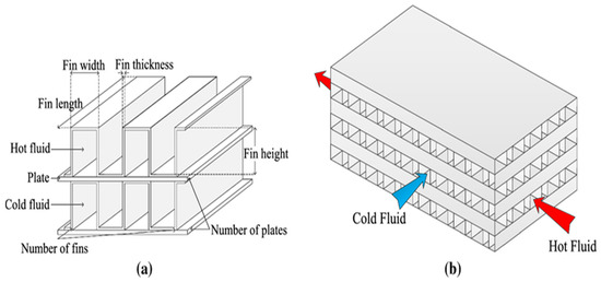
Figure 1 illustrates a conventional two-stream straight-finned plate–fin heat exchanger. The design parameters shown in Figure 1a correspond to the plate–fin segment of the heat exchanger. In general, thin aluminum plates are brazed together to form the fins, resulting in a relatively simple fin geometry. The operating principle of the plate–fin heat exchanger is presented in Figure 1b [32]. In order to achieve efficient heat exchange, the two working fluids flow alternately through separate fin passages. The plate–fin heat exchanger configuration shown in Figure 1 serves as the basis for the optimization study presented in this work. Based on this configuration, the governing equations are derived, followed by the formulation of optimization objectives and constraints [33].

Symbol	Description	Unit
Cp	Specific heat capacity	J·kg−1·K−1
m	Mass flow rate	kg·s−1
$∆P$	Pressure drop	Pa
Re	Reynolds number	-
Nu	Nusselt number	-
f	Friction factor	-
Q	Heat transfer rate	W
$\epsilon$	Heat exchanger effectiveness	-

Figure 1. (a) Plate–fin heat exchanger and (b) Rectangular offset strip fin (Figure is taken from the ref. [34]).

2.1. Plate–Fin Heat Exchanger Formula Derivation

The heat duty $Q$ of the heat exchanger is first determined using the formulation proposed by Yousefi et al. [35], which represents the overall energy exchange capacity of the system:

$$Q=ϵC_{min}\left(T_{Ain}-T_{Bin}\right)$$

(1)

$$C_{min}=m \ast C_p$$

(2)

where C denotes the heat capacity rate; the subscripts A and B refer to the hot and cold fluids, respectively; the subscript $in$ indicates the inlet condition; $min$ represents the smaller heat capacity rate of the two fluids; and $max$ corresponds to the larger heat capacity rate.

The effectiveness is given by Incropera et al. [36],

$$ϵ=1-e^{\left(\left({\displaystyle \frac{1}{C_r}}\right){NTU}^{0.22}\left(e^{\left(-C_r{NTU}^{0.78}\right)}-1\right)\right)}$$

(3)

where $e$ is the Eulers number,

$$C_r=C_{min}/C_{max}$$

(4)

A popular thermodynamic solution technique for cases where the outlet temperature is unknown is the heat transfer coefficient method. The following is the expression for the heat transfer coefficient:

$${\displaystyle \frac{1}{NTU}}=C_{min}({\displaystyle \frac{A_{ffA}}{j_{A}C{p}_{A}P{r}_A^{-0.667}{m}_h{A}_A}}+{\displaystyle \frac{A_{ffB}}{j_{B}C{p}_{B}P{r}_B^{-0.667}{m}_B{A}_B}})$$

(5)

where $A$, $A_{HT}$ is the heat transfer area $\left({\mathrm{m}}^2\right)$, $C_p$ is the fluid’s specific heat $\left(\mathrm{J}{\mathrm{k}\mathrm{g}}^{-1}{\mathrm{K}}^{-1}\right)$, and $j$ is the Colburn factor, $N_S$ is the number of entropy generating units, and $Pr$ is the Prandtl number.

The definition of two fluids’ free flow area is

$${Aff}_A=(H_t-t_A)(1-n_A{t}_A)L_B{N}_A$$

(6)

$${Aff}_B=(H_B-t_B)(1-n_B{t}_B)L_A{N}_B$$

(7)

In the equation, $H$ represents the fin height, $t$ indicates the fin thickness, $n$ signifies the fin frequency, $L$ refers to the length of the heat exchanger, $N$ denotes the number of fin layers, $\mu$ stands for dynamic viscosity (measured in $\left(\mathrm{k}\mathrm{g}{\mathrm{s}}^{-1}{\mathrm{m}}^{-1}\right)$), and ρ represents density (expressed in $\left(\mathrm{k}\mathrm{g}{\mathrm{m}}^{-3}\right)$).

Fluid B possesses an additional layer compared to Fluid B itself:

$$N_B=N_A+1$$

(8)

The expression for the fluid’s heat transfer area is adopted from the work of Yousefi [37].

$$A_A=L_A{L}_B{N}_A(1+(2n_A(H_A-t_A)))$$

(9)

$$A_B=L_A{L}_B{N}_A(1+(2n_B(H_B-t_B)))$$

(10)

The Colburn factor is represented by $j$, while $f$ denotes the Fanning friction factor [38].

For laminar flow conditions $(Re\le 1500)$,

$$j=0.53{\left(Re\right)}^{-0.5}{\left({\displaystyle \frac{l}{D_h}}\right)}^{-0.15}{({\displaystyle \frac{s}{H}}-t)}^{-0.14}$$

(11)

$$j=8.12{\left(Re\right)}^{-0.74}{\left({\displaystyle \frac{l}{D_h}}\right)}^{-0.41}{({\displaystyle \frac{s}{H}}-t)}^{-0.02}$$

(12)

For turbulent flow $(Re>1500)$,

$$j=0.21{\left(Re\right)}^{-0.4}{\left({\displaystyle \frac{l}{D_h}}\right)}^{-0.24}{({\displaystyle \frac{s}{H}}-t)}^{0.02}$$

(13)

$$j=1.12{\left(Re\right)}^{-0.36}{\left({\displaystyle \frac{l}{D_h}}\right)}^{-0.65}{({\displaystyle \frac{s}{H}}-t)}^{0.17}$$

(14)

Here, $Re$ stands for the Reynolds number, and $s$ represents the fin spacing.

The fin spacing of the plate–fin heat exchanger (PFHE):

$$s=({\displaystyle \frac{1}{n}}-t)$$

(15)

where

$$Re={\displaystyle \frac{m.D_h}{A_{ff}\mu }}$$

(16)

The hydraulic diameter $D_h$ of the heat exchanger, based on the fin configuration outlined in this study, can be expressed as follows:

$$D_h={\displaystyle \frac{4s(H-t)l}{2\left(sl+\left(H-t\right)l+t\left(H-t\right)\right)+ts}}$$

(17)

Here, $l$ represents the lance length of the fin, while $D_h$ denotes its hydraulic diameter.

The following formula can be used to determine the pressure decrease brought on by friction between the fin and the channel’s fluid:

$$∆P_A={\displaystyle \frac{2f_A{L}_A{\left(\frac{m_A}{{Aff}_A}\right)}^2}{{\rho }_A{D}_{h,A}}}$$

(18)

$$∆P_B={\displaystyle \frac{2f_B{L}_B{\left(\frac{m_B}{{Aff}_B}\right)}^2}{{\rho }_B{D}_{h,B}}}$$

(19)

where $∆P$ is pressure drop $\left(\mathrm{N}{\mathrm{m}}^{-2}\right).$ Equations (15)–(19) are adopted from Incropera et al. [36] and Yousefi et al. [35].

In this study, the pressure drop is evaluated under the assumption of a constant mass flow rate, which is a common design condition in compact heat exchanger applications where flow rates are prescribed by upstream system requirements such as compressors or fans. Under constant mass flow conditions, pumping power is directly proportional to pressure drop, and therefore minimizing pressure loss is equivalent to reducing pumping energy consumption up to a constant proportionality factor. This formulation enables a fair comparison of different geometric configurations without introducing additional system-dependent parameters such as pump efficiency. Consequently, pressure drop is adopted as an appropriate hydraulic performance indicator for the present optimization framework.

2.2. Objective Functions of the Plate–Fin Heat Exchanger

During fluid flow through heat exchanger channels, frictional effects lead to entropy generation. The magnitude of entropy generation is strongly influenced by the geometric design of the heat exchanger. Lower entropy generation indicates improved thermodynamic performance under identical operating conditions. Consequently, entropy generation is considered an effective performance evaluation index in heat exchanger optimization.

The entropy generation number is defined as the first objective function [39]:

$$Ns=\left(1-ϵ\right)\left[{\displaystyle \frac{{\left(T_{Bin}-T_{Ain}\right)}^2}{T_{Bin}{T}_{Ain}}}\right]+\left({\displaystyle \frac{Rct{e}_A}{C{p}_A}}\right)\left({\displaystyle \frac{∆P_A}{P_{Ain}}}\right)+\left({\displaystyle \frac{Rct{e}_B}{C{p}_B}}\right)\left({\displaystyle \frac{∆P_B}{P_{Bin}}}\right)$$

(20)

In this context, $Rcte$ refers to the specific gas constant, expressed in units of $\left(\mathrm{J}{\mathrm{k}\mathrm{g}}^{-1}{\mathrm{K}}^{-1}\right)$.

In addition to entropy generation, the effective heat transfer area is an important indicator of heat exchanger performance, as it directly affects heat transfer efficiency and Reynolds number. Therefore, following the approach in [40], the total heat transfer area is considered as the second objective function in this study:

$$A_{HT}=A_A+A_B$$

(21)

2.3. PFHE Application Example

Two plate–fin heat exchanger design cases are investigated in this study, differing in geometric constraints and fluid operating conditions. The corresponding design limits and fluid properties are summarized in Table 1.

Table 1. Parameters and properties.

Parameters	Project 1		Project 2
	Lower Bound	Upper Bound	Lower Bound	Upper Bound
Fluid A, heat exchanger length, m	0.1	1	0.1	1
Fluid B, heat exchanger length, m	0.1	1	0.1	1
The fin’s height, m	0.002	0.01	0.002	0.01
The frequency of fins	100	1000	100	1000
Fin thickness, m	0.0001	0.0002	0.0001	0.0002
The fin’s Lance length, m	0.001	0.01	0.001	0.01
The quantity of fin layers	1	10	1	200
Parameters	Project 1		Project 2
	Fluid A	Fluid B	Fluid A	Fluid B
Heat exchanger length, m, Fluid A	0.8962	0.8296	1.66	2
Heat exchanger length, m, Fluid B	513	277	1173.15	473.15
Height of the fin, m	100,000	100,000	160,000	200,000
Fin frequency	1017.7	1011.8	1122	1073
Fin thickness, m	0.8196	0.9385	0.6296	0.9638
The fin’s Lance length, m	2.410 × 10−5	2.182 × 10−5	4.010 × 10−5	3.360 × 10−5
Number of fin layers	0.6878	0.6954	0.731	0.694

To ensure that the heat duty requirements are satisfied, penalty functions are incorporated into the optimization process. The penalty function formulation is expressed as:

$$g\left(X\right)⟹\xi \left(X\right)-Q=0$$

(22)

The design constraints include the overall dimensions of the heat exchanger, fin geometry (length, width, height, and thickness), fin density, and the number of fluid layers on each side. In Case 1, the required heat duty is set to 160 kW, while in Case 2 it is 1050 kW. The overall heat exchanger volume is constrained to $1 \mathrm{m}\times 1 \mathrm{m}$. For simulation purposes, both working fluids are modeled as ideal gases [41].

2.4. Challenges in Optimizing Plate–Fin Heat Exchangers

Plate–fin heat exchangers are extensively employed in aerospace, cryogenics, and chemical processing due to their compact structure and high thermal efficiency. However, optimizing their performance presents several challenges, particularly in balancing thermal enhancement and hydraulic losses. The complex fin geometry and narrow flow channels result in intricate flow patterns, which may cause flow maldistribution. Such maldistribution reduces heat transfer effectiveness while increasing pressure drop, thereby degrading overall energy efficiency.

Furthermore, different fin configurations—including plain, offset, and serrated fins—introduce trade-offs between maximizing heat transfer surface area and minimizing hydraulic resistance. Although computational fluid dynamics (CFD) tools are valuable for analyzing these effects, their high computational cost limits rapid design iterations. Material selection further complicates the optimization process, as thermal conductivity, corrosion resistance, and mechanical durability must be simultaneously satisfied.

Mechanical and structural constraints pose additional challenges, particularly under high-pressure and high-temperature operating conditions. Thin fins and brazed joints, while beneficial for heat transfer, are vulnerable to thermal stresses, fatigue, and vibration-induced damage. Reducing fin thickness may enhance thermal performance but can compromise structural integrity, necessitating multi-objective optimization approaches. Moreover, fouling and corrosion caused by aggressive working fluids can degrade long-term performance, while maintenance and inspection are difficult due to the compact and sealed nature of PFHEs.

Manufacturing limitations and cost considerations further restrict practical design optimization. Precision fabrication techniques such as vacuum brazing or diffusion bonding are required to ensure structural integrity, but these processes are sensitive to material impurities and dimensional tolerances. Small deviations in fin alignment or bonding quality can significantly affect performance, while advanced materials and complex geometries often increase production costs. These challenges highlight the need for integrated optimization strategies that simultaneously address thermal performance, structural reliability, manufacturability, and economic feasibility.

3. Algorithm Preliminaries

Heuristic optimization techniques are inspired by principles from natural sciences such as mathematics, physics, and biology. Each algorithm is characterized by unique particle updating mechanisms, which define its specific features. Depending on the underlying concept, some algorithms may require tuning multiple parameters, such as four or six, to achieve optimal performance, while others operate effectively without such adjustments.

Aquila optimizer (AO)

The Aquila Optimizer (AO) is a metaheuristic algorithm modeled after the hunting strategies of the Aquila bird species [19]. The AO replicates the four primary strategies employed by the bird to seize its prey. For instance, the Aquila leverages its elevated position to descend sharply in a vertical dive, snatching unsuspecting prey from the water’s surface. When pursuing seabirds, the Aquila skims near the ground in a contour-hugging flight, executing rapid glide-based attacks. This approach is also used by the Aquila bird to target foxes and other less agile prey. Through this method, the bird can traverse the terrain on foot, swiftly apprehending its target.

3.1. First Stage Exploration

The Aquila Optimizer (AO) algorithm reflects the Aquila bird’s extensive exploration during hunting. It begins with strong exploration, surveying the search space to locate potential solutions (prey) and target the best area for focus. Equation (23) in [19] mathematically describes this initial phase.

$$X_I^{t+1}=X_{best}^t\times \left(1-{\displaystyle \frac{t}{T}}\right)+(X_M^t-rand\times X_{best}^t)$$

(23)

In the AO algorithm, $T$ denotes the total number of iterations, while $t$ represents the current iteration. The term $X_I^{t+1}$ refers to the candidate solution for the next iteration, generated during the initial population search. $X_{best}^t$ indicates the best solution found up to the $i^{th}$ iteration, and the expression $(1-{\displaystyle \frac{t}{T}})$ reflects the influence of the global search throughout the optimization process. Here, $N$ is the size of the population, $Dim$ refers to the dimensionality of the problem, and $X_M^t$ represents the mean position of all solutions at the $i^{th}$ iteration, as defined in Equation (24).

$$X_M^t={\displaystyle \frac{1}{N}}{\sum }_{i=1}^N{X}_i\left(t\right), \forall i=\mathrm{1,2},\dots , Dim$$

(24)

3.2. Second Stage Exploration

The Aquila Optimizer’s $X_2$ method employs a focused exploration strategy, mirroring the Aquila bird’s hunting technique of flying in a contour-like pattern and executing rapid gliding attacks within a limited area to catch prey. This approach, outlined in Equation (25), aims to determine the solution $X_2^{t+1}$ for each of the following h iterations.

$$X_2^{t+1}=X_{best}^t\times Levy\left(Dim\right)+X_R^t+(v-u)\times rand$$

(25)

In this context, $[1,N]$, represents the range, with $N$ indicating the population size, $X_R^t$ signifying the random solution obtained at the $i^{th}$ iteration, and s set as a constant at 0.01. Parameters $u$ and $v$ are randomly selected values between 0 and 1. The mathematical formula for this calculation is provided in Equation (26).

$$Levy\left(Dim\right)=s\times {\displaystyle \frac{u\times \sigma }{{\left|v\right|}^{\frac{1}{a}}}}$$

(26)

Equation (27) calculates the value of $\sigma$ using the constant parameter $a$, fixed at $1.5$.

$$\sigma =({\displaystyle \frac{\gamma (1+a)\times \mathrm{s}\mathrm{i}\mathrm{n}\left(\frac{\pi a}{2}\right)}{\gamma \left(\frac{1+a}{2}\right)\times a\times 2^{\left(\frac{a-1}{2}\right)}}}$$

(27)

Equations (28) and (29) depict the spiral shape that falls inside the search range, denoted by $v$ and $u$, respectively. Equation (25) specifies this spiral shape.

$$v=r_1+{UD}_1\cos \left(-\omega D_1+({\displaystyle \frac{3\pi }{2}})\right)$$

(28)

$$u=r_1+{UD}_1\sin \left(-\omega D_1+({\displaystyle \frac{3\pi }{2}})\right)$$

(29)

The values of the variable $r_1$, range from 1 to 20 over a predetermined number of search iterations. $\omega$ and $U$ will always be $0.005$ and $0.00565$, respectively. The dimension $Dim$ of the search space has a range of $1$ to $D_1\in \mathbb{Z}$.

3.3. First Stage Exploitation

An extended exploitation $X_3^{t+1}$ approach is incorporated into the algorithm to mimic the Aquila bird’s careful prey inspection prior to striking. This phase enables a more in-depth examination of promising regions within the search space and is mathematically represented by Equation (30).

$$X_3^{t+1}={(X}_{best}^t-X_M^t)\times \theta -rand+((ub-lb)\times rand+lb)\times \rho$$

(30)

In this context, $X_3^{t+1}$ denotes the result of the subsequent iteration, while $X_M^t$ refers to the average value of the current population, determined using Equation (24) at the $i^{th}$ iteration. $X_{best}^t$ represents the best solution identified up to that point. The control parameters $\theta$ and $\rho$ are both set to 0.1. The term rand signifies a randomly generated number within the range [0, 1], and $ub$ and $lb$ correspond to the upper and lower bounds of the search space, respectively.

3.4. Second Stage Exploitation

The second stage exploitation strategy in the Aquila Optimizer algorithm is inspired by the hunting techniques employed by Aquila birds. These birds directly capture their prey by taking advantage of its unpredictable ground movements. Equation (31), which represents the design of the constrained exploitation technique $X_4^t$, reflects this approach. The $i^{th}$ iteration of the answer, represented as $X_4^{t+1}$, is also produced by this equation. Equation (32) presents the quality function $J$ in order to preserve a balanced search strategy.

$$X_4^{t+1}=J\times X_{best}^t-\left(P_1\times rand\times X_1^t\right)-P_2\times Levy\left(Dim\right)+rand\times P_1$$

(31)

$$J\left(t\right)=t^{{\displaystyle \frac{2\times rand-1}{{\left(1-T\right)}^2}}},$$

(32)

Equations (33) and (34) are employed to compute the motion pattern of the Aquila’s prey pursuit $\left(P_1\right)$ and the path of a strike during an escape, from the initial to the final point $\left(P_2\right)$. These computations incorporate the current iteration t and the total number of iterations $T$. The expressions are defined as follows:

$$P_1=2\times rand-1,$$

(33)

$$P_2=2\times (1-{\displaystyle \frac{t}{T}})$$

(34)

The pseudocode outlined in Algorithm 1 offers an overview of the Aquila Optimizer process.

Algorithm 1 Aquila Optimizer (AO)

Initialize the parameter and generate initial population randomly. While t < T      Calculate the fitness of each solution      Find the best solution so far      For each aquila $X_i$              If $t\le \left({\displaystyle \frac{2}{3}}\right)\times T$ then                   if $rand\le 0.5$                       Apply Equation (23)                   Else                       Apply Equation (25)                   End if              Else                   If $rand\le 0.5$                       Apply Equation (30)                   Else                       Apply Equation (31)                   End if              End if      End For      $t=t+1$ End While Obtain the best position

However, despite its high search efficiency and strong exploratory capabilities, the Aquila optimiser regularly encounters serious problems like skips of real solutions and local optima stagnation. Consequently, AO’s search approach needs to be enhanced. The current endeavour aims to improve the efficiency of classical AO.

4. The Proposed Modified Aquila Optimizer (m-AO) Algorithm

This study introduces three enhancement strategies to improve the performance of the standard Aquila Optimizer (AO). The proposed modifications are designed to overcome the primary limitations of AO, namely insufficient population diversity, imbalance between exploration and exploitation, and slow convergence. Specifically, an adaptive chaotic reverse learning strategy is employed to enhance population diversity, an elite alternative pooling mechanism is introduced to balance exploration and exploitation, and a shifted distribution estimation strategy is incorporated to guide the evolutionary trajectory. The detailed descriptions of these three strategies are provided in the following subsections.

4.1. Adaptive Chaotic Reverse Learning Strategy

One of the inherent limitations of metaheuristic optimization algorithms is the gradual loss of population diversity as iterations progress, which often leads to premature convergence. To address this issue, various diversity-preservation techniques have been proposed, among which reverse learning has proven to be particularly effective. Reverse learning is based on the principle that reverse solutions have approximately a 50% probability of being closer to the global optimum than the original solutions. Consequently, this strategy has been successfully applied to enhance the performance of several optimization algorithms [42,43,44]. The reverse learning mechanism can be mathematically expressed as follows:

$$X_i^o=LB+UB-X_i^t,$$

(35)

The reverse solution to $X_i^t$ is represented as $X_i^o$. Population diversity is closely related to the distribution of individuals within the search space. A more uniform distribution generally indicates higher diversity. Chaotic maps possess two essential characteristics—randomness and ergodicity—which enable optimization algorithms to explore the search space more effectively and reduce the likelihood of premature convergence. These properties have been shown to significantly improve the performance of various metaheuristic algorithms [45]. In this study, a chaotic reverse learning strategy is proposed by integrating chaotic mapping with reverse learning. The chaotic reverse solution is generated as

$$X_i^{co}=LB+UB-{{\lambda }_{i}X}_i^t,$$

(36)

In the chaotic reverse learning mechanism, the solution generated for the $i^{th}$ individual is denoted as $X_i^{co}$, where ${\lambda }_i$ represents the corresponding chaotic map value. Table 1 presents the equations and probability distributions of the ten most commonly used chaotic maps. The quality of the initial population plays a critical role in determining the convergence behavior of swarm intelligence algorithms. To enhance the diversity of the initial population and improve convergence accuracy, the Chaotic Opposition-Based Learning (COBL) method is employed during population initialization. Furthermore, at each iteration, a corresponding reverse population is generated using COBL and evaluated independently. The best-performing individuals are then retained for the subsequent generation.

To reduce computational overhead and avoid inefficiencies associated with applying chaotic reverse learning to all individuals, a linearly decreasing population strategy is introduced [46]. As iterations proceed, the number of individuals subjected to chaotic reverse learning gradually decreases. The formulation of this strategy is given by

$$Pop=round({\displaystyle \frac{\left({pop}_{min}-{pop}_{max}\right)·t}{T}}+{pop}_{max})$$

(37)

Here, ${pop}_{max}$ and ${pop}_{min}$ represent the highest and lowest population sizes, respectively, while $Pop$ denotes the current population size determined using the chaotic backward learning method.

4.2. Elite Alternative Pooling Strategy

In the original AO algorithm, position updates are guided primarily by the global best individual. While this approach accelerates convergence, it also reduces population diversity and increases the risk of stagnation in local optima. To mitigate this issue, an elite alternative pooling strategy is proposed to achieve a more balanced trade-off between exploration and exploitation [47].

In this strategy, the top three individuals in the current population are stored in an elite pool, as defined by

$$X_{eap}=\{X_{eap1},X_{eap2},X_{eap3}\}$$

(38)

where the top three people in the population so far are $X_{eap1}$, $X_{eap2}$, and $X_{eap3}$. Each time, one of these three people is randomly selected as the food source. By selecting the guiding solution from multiple elite candidates rather than relying solely on the global best, the algorithm reduces the likelihood of premature convergence and improves its ability to escape local optima. To further enhance convergence efficiency, globally optimal individuals are also incorporated into the elite pool. This mechanism enables all individuals in the population to benefit from high-quality solution information while maintaining sufficient diversity.

The final mathematical formulation of the elite alternative pooling strategy is expressed as

$$X_{eap}=\{X_{eap1},X_{eap2},X_{eap3},X_{best}\}$$

(39)

4.3. Shifted Distribution Estimation Strategy

In the standard AO algorithm, the search process is predominantly driven by the best individual, which may result in the underutilization of valuable information contained in other high-quality solutions. To address this limitation, distribution estimation strategies have been introduced in several studies to exploit the statistical characteristics of dominant populations [48,49].

Distribution estimation methods construct a probabilistic model based on elite individuals and generate new candidate solutions by sampling from this model. This study proposes a shifted distribution estimation strategy that incorporates both the dominant population and the best individual to guide the evolutionary process more effectively.

The mathematical formulation of the proposed strategy is given by

$$X_i^{t+1}=mean+y, \hspace{1em}y~N\left(0,Cov\right),$$

$$mean={\displaystyle \frac{\left(X_{best}^t+X_{mean}^t+X_i^t\right)}{3}},$$

$$Cov\left(i\right)={\displaystyle \frac{1}{\frac{NP}{2}}}\sum _{i=1}^{{\displaystyle \frac{NP}{2}}}(X_i^{t+1}-X_{mean}^t)\times {\left(X_i^t-X_{mean}^t\right)}^T,$$

$$X_{mean}^t=\sum _{i=1}^{NP/2}{\omega }_i\times X_i^t,$$

$${\omega }_i={\displaystyle \frac{\ln \left(0.5NP+0.5\right)-\mathrm{l}\mathrm{n}\left(i\right)}{{\sum }_{i=1}^{NP/2}(\ln \left(0.5NP+0.5\right)-\ln \left(i\right))}}$$

(40)

Here, ${\omega }_i$ denotes the weight coefficient allocated to the dominant individuals within the population, ranked in descending order according to their fitness scores. $X_{mean}^t$ represents the weighted average position of this elite group, while $Cov$ signifies the weighted covariance matrix corresponding to the dominant population. The overall workflow of the proposed m-AO algorithm is illustrated in Figure 1, and its corresponding pseudocode is provided in Algorithm 2.

Algorithm 2 Modified Aquila Optimizer (m-AO)

Set up initial parameters and randomly create the starting population. While $t<T$        Compute the fitness value for each solution and build the elite alternative        search pool using Equation (17)        Identify the best solution found so far        Determine the mean and covariance based on Equation (18)        For each aquila $X_i$ do               If $t\le ({\displaystyle \frac{2}{3}})\times T$ then                    If $rand<0.5$                        If $rand\le 0.5$                            Implement Equation (23)                        Else                            Implement Equation (25)                        End if                    Else                        If $rand\le 0.5$                            Implement Equation (30)                        Else                            Implement Equation (31)                        End if                    End if               Else                    Compute the updated position $X_i$ using Equation (18)               End if           Evaluate the fitness and retain the superior solution           Refresh the population using Equation (15)           Determine the new position $X_i$ using Equation (14)           Assess the fitness and keep the better solution           End For Increment t by 1 (t = t + 1) End While Retrieve the optimal position

Despite the improved performance demonstrated by the proposed modified Aquila Optimizer (m-AO), several limitations should be acknowledged. First, the plate–fin heat exchanger optimization problem is formulated using empirical heat transfer and pressure drop correlations. While these correlations are well established in the literature, they may not fully capture complex three-dimensional flow effects, secondary flows, or local heat transfer phenomena that can be observed in high-fidelity computational fluid dynamics (CFD) simulations.

Second, the proposed optimization framework does not explicitly account for long-term operational factors such as fouling resistance, material degradation, or thermal expansion effects. These factors may influence the long-term performance and reliability of plate–fin heat exchangers in practical industrial environments.

Third, like most metaheuristic algorithms, the m-AO is inherently stochastic. Although statistical tests confirm its robustness and consistency, slight variations in the obtained solutions may occur across different runs. Consequently, multiple independent executions are recommended to ensure solution reliability, especially for highly constrained or sensitive design problems.

Finally, the current study focuses on single-objective optimization scenarios under fixed boundary conditions. Multi-objective formulations involving simultaneous optimization of thermal performance, pressure drop, cost, and mechanical reliability were not considered and represent a promising direction for future investigation.

4.4. Computational Complexity Analysis

Analyzing computational complexity is essential for evaluating the efficiency of optimization algorithms. Let $N$ denote the population size, $Dim$ the problem dimension, and $T$ the maximum number of iterations. In each iteration, m-AO performs fitness evaluation for all individuals, constructs the elite pool, computes statistical parameters, and updates solution positions through exploration, exploitation, or distribution estimation strategies. The fitness evaluation and solution updates typically involve operations with a time complexity of $O\left(Dim\right)$, while constructing the elite pool may require sorting, resulting in an additional $O\left(NlogN\right)$. Moreover, if full covariance matrices are used, the computation cost can increase to $O(N\times D^2)$. Therefore, the overall time complexity of the algorithm is approximately $O(T\times \left(N\times {Dim}^2+NlogN\right))$. However, if simplified (diagonal) covariance matrices are assumed and the fitness function is linear in $Dim$, the time complexity reduces to $O(T\times N\times Dim)$, making the algorithm computationally efficient for large-scale problems.

5. Performance Analysis of m-AO

Comprehensive tests were carried out to evaluate the optimization abilities and effectiveness of the proposed m-AO. The m-AO algorithm was implemented using MATLAB R2023a on a system equipped with an Intel Core i5 11300H processor, operating at 3 GHz and 10 GHz, and supported by 16 GB of RAM.

Section 5.1 contains comprehensive details regarding these benchmark functions while Section 5.2 introduces the parameter settings of competitive algorithms. The efficacy of proposed m-AO is assessed on classical [50] and CEC’22 benchmark functions [51] in Section 5.3 and Section 5.4, respectively. Section 5.5 presents the statistical test including Friedman test and Wilcoxon signed rank test [52,53].

5.1. CEC Benchmark Functions

The performance of the proposed m-AO was evaluated using two benchmark collections: the Classical suite and the CEC’22 suite. The Classical benchmark [50] includes 23 test functions, covering diverse categories such as unimodal, multimodal, and fixed-dimensional multimodal functions. A detailed summary of these functions is provided in Table 2. In contrast, the CEC’22 test suite features 12 test functions, which span unimodal, basic, hybrid, and composition types. Table 3 presents an in-depth description of the CEC’22 benchmark functions.

Table 2. Overview of classical benchmark function characteristics (Dim = 30).

Type	ID	Description	Range	Dim	F_min
Unimodal, Separable	C1	Sphere	[−100, 100]	30	0
Unimodal Non-separable	C2	Schwefel 2.22	[−10, 10]	30	0
Unimodal Non-separable	C3	Schwefel 2.21	[−100, 100]	30	0
Unimodal, Separable	C4	Schwefel 2.21	[−100, 100]	30	0
Unimodal Non-separable	C5	Rosenbrock	[−30, 30]	30	0
Unimodal, Separable	C6	Step	[−100, 100]	30	0
Unimodal, Separable	C7	Quartic	[−1.28, 1.28]	30	0
Multimodal, Separable	C8	Schwefel 2.26	[−500, 500]	30	418.9829
Multimodal, Separable	C9	Rastrigin	[−5.12, 5.12]	30	0
Multimodal, Separable	C10	Ackley	[−32, 32]	30	8.8818 × 10−16
Multimodal, Non-separable	C11	Griewank	[−600, 600]	30	0
Multimodal, Non-separable	C12	Penalized	[−50, 50]	30	0
Multimodal, Non-separable	C13	Penalized 2	[−50, 50]	30	0
Multimodal, Separable	C14	Foxholes	[−65.53, 65.53]	2	0.998004
Multimodal, Separable	C15	Kowalik	[−5, 5]	4	0.0003075
Multimodal, Non-separable	C16	Six-hump camel back	[−5, 5]	2	1.03163
Multimodal, Separable	C17	Branin	[−5, 10]*[0, 15]	2	0.398
Multimodal, Non-separable	C18	Goldstein-Price	[−5, 5]	2	3
Multimodal, Non-separable	C19	Hartman 3	[0, 1]	3	3.8628
Multimodal, Non-separable	C20	Hartman 6	[0, 1]	6	3.32
Multimodal, Non-separable	C21	Langermann 5	[0, 10]	4	10.4029
Multimodal, Non-separable	C22	Langermann 7	[0, 10]	4	10.4029
Multimodal, Non-separable	C23	Langermann 10	[0, 10]	4	10.5364

Table 3. Overview of CEC’22 benchmark function characteristics.

Type	ID	Description	Range	Dim	F_min
Unimodal Multimodal	C1 C2 C3 C4 C5	Shifted and Full Rotated Zakharov Function Shifted and Full Rotated Rosenbrock’s Function Shifted and Full Rotated Rastrigin’s Function Shifted and Full Rotated Non-Continuous Rastrigin’s Function Shifted and Full Rotated LevyFunction	[−100, 100] [−100, 100] [−100, 100] [−100, 100] [−100, 100]	20 20 20 20 20	300 400 500 600 700
Hybrid	C6 C7 C8	Hybrid Function 1 (N = 3) Hybrid Function 2 (N = 4) Hybrid Function 3 (N = 5)	[−100, 100] [−100, 100] [−100, 100]	20 20 20	800 900 1000
Composition	C9 C10 C11 C12	Composition Function 1 (N = 5) Composition Function 2 (N = 3) Composition Function 3 (N = 6) Composition Function 4 (N = 6)	[−100, 100] [−100, 100] [−100, 100] [−100, 100]	20 20 20 20	2000 2100 2200 2300

5.2. Parameter Settings of Competitive Algorithms

It is essential to use well-known intelligent optimization algorithms as a base line for comparison to ensure a fair and comprehensive analysis. Seven well known and latest popular MAs are selected which are Grasshopper optimization algorithm (GOA) [54], Particle Swarm Optimization (PSO) [55], Whale Optimization Algorithm (WOA) [56], and Grey Wolf Optimizer (GWO) [57], Crayfish Optimization Algorithm (COA) [58], Harris Hawk Optimization Algorithm (HHO) [59], and the original Aquila Optimizer (AO) [19]. Table 3 displays the parameter settings of these MAs. Table 4 presents the parameter settings of the algorithms.

Table 4. Parameters of MAs.

Algorithm	Proposed Year	Parameters
AO	2021	$U=0.00565, R=10, w=0.005, \alpha , \beta =0.1$
GWO	2014	$a=\left[\mathrm{2,0}\right]$
PSO	1995	$c_1=c_2=2, v=6$
WOA	2016	$a_1=\left[\mathrm{2,0}\right], a_2=\left[-1,-2\right],b=2$
COA	2023	$c=\left[\mathrm{2,0}\right], temp=\left[\mathrm{20,35}\right]$
GOA	2017	$f=0.5, l=1.5, c_{max}=1, c_{min}=0.0004$
HHO	2019	$E\in \left[\mathrm{0,2}\right]$
EDOLSCA	2021	$b=2$

In the simulation setup, the initial population size (N) for all algorithms is fixed at 30, and the maximum number of iterations (T) is set to 1000. Since metaheuristic methods are inherently stochastic, the results from a single run may not be reliable. To mitigate the impact of random factors, each algorithm is executed 10 times. The main evaluation metrics include the average value (Mean) and the standard deviation (StdDev) of the results obtained from 10 runs.

5.3. Classical Benchmark Function Simulation Results

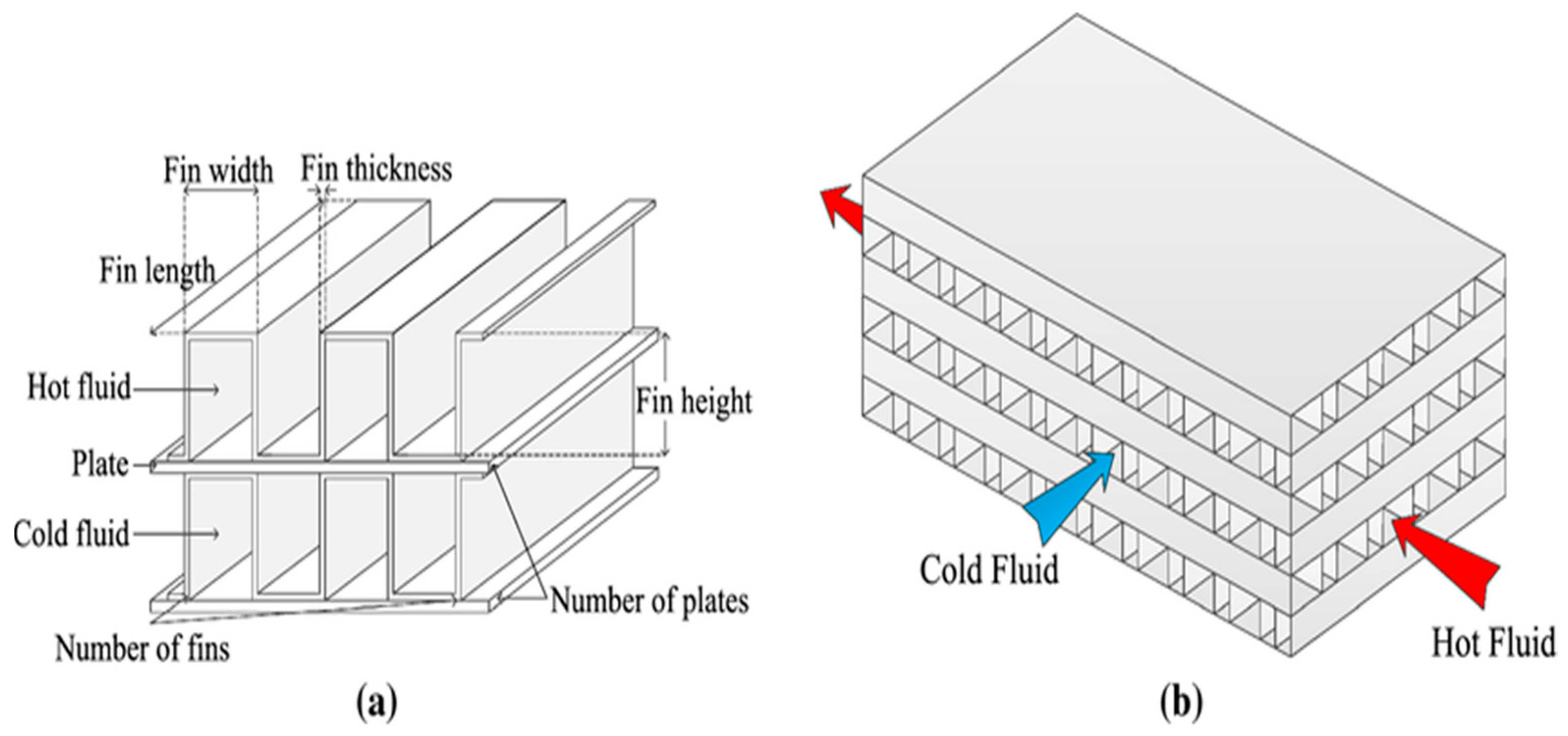
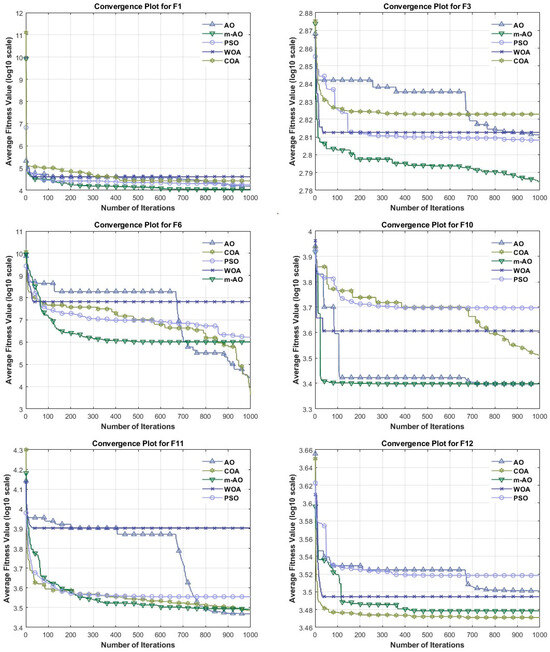
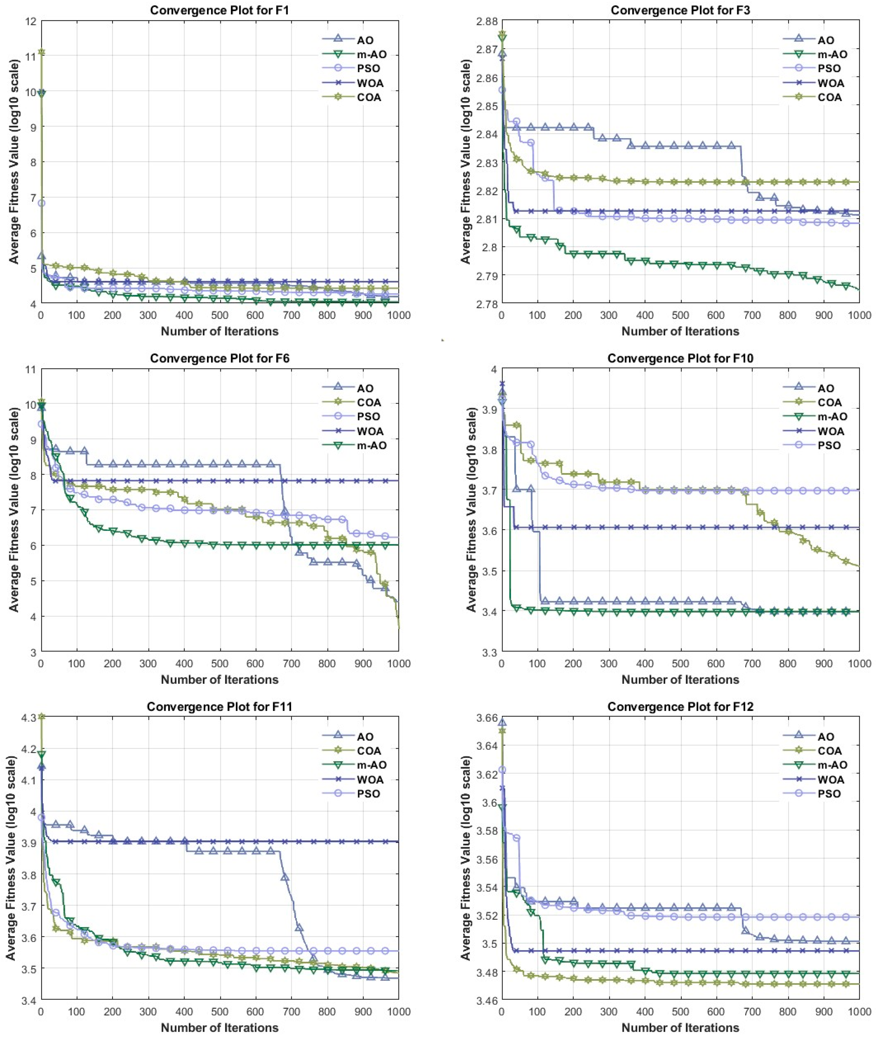
Table 5 reports the statistical results such as Mean, StdDev, and Friedman ranking test for the proposed m-AO algorithm and other compared algorithms for each Classical benchmark function. Certain conclusions can be drawn from this table. The proposed m-AO algorithm achieves the global optimal solution (best optimal solutions) for the 23 functions including C1–C11, C13–C17, C20–C23. Additionally, m-AO demonstrates the second-best performance for functions C12, C18, and C19. The effectiveness of the improvements made to the basic AO is demonstrated by these results, which show that m-AO performs better than other approaches on the majority of test functions. m-AO and competing algorithms’ convergence curves on the classical benchmark functions are depicted in Figure 2. This shows that the changes made to the original AO were effective. When compared to other algorithms, m-AO likewise shows quick convergence and produces extremely accurate optimal solutions for other functions.

Table 5. Mean and standard deviation results for classical unimodal and multimodal test functions.

Test Function		AO	PSO	WOA	GWO	COA	m-AO
C1	Mean STD	0.00 0.00	1.67 × 10−27 2.59 × 10−27	1.04 × 10−19 1.43 × 10−19	7.03 × 10−27 5.58 × 10−27	1.49 × 10−69 2.403 × 10−69	0.00 0.00
C2	Mean STD	1.28 × 10−216 0.00 × 100	1.82 × 10−17 2.32 × 10−17	1.412 × 10−19 3.15 × 10−19	1.83 × 10−9 2.27 × 10−9	1.224 × 10−49 1.445 × 10−49	0.00 0.00
C3	Mean STD	0.00 × 100 0.00 × 100	2.43 × 10−5 3.72 × 10−5	4.19 × 10−6 3.76 × 10−5	1.44 × 10−4 2.52 × 10−4	1.704 × 10−3 4.39 × 10−3	0.00 0.00
C4	Mean STD	1.17 × 10−217 0.00 × 100	2.49 × 10−4 3.74 × 10−4	3.15 × 101 4.05 × 101	2.14 × 10−7 2.55 × 10−7	1.07 × 10−6 1.56 × 10−6	0.00 0.00
C5	Mean STD	7.27 × 10−3 7.15 × 10−3	4.92 × 101 2.84 × 101	7.65 × 100 8.26	6.99 × 101 0.68312	2.71 × 10−3 0.75046	2.06 × 10−7 3.81 × 10−7
C6	Mean STD	1.09 × 10−3 1.65 × 10−3	4.11 × 10−4 3.28 × 10−4	5.02 × 10−1 1.03 × 10−1	3.59 × 10−1 0.35208	7.246 × 10−1 0.3653	7.029 × 10−9 4.533 × 10−9
C7	Mean STD	5.31 × 10−4 5.12 × 10−4	9.41 × 10−3 4.36 × 10−3	5.21 × 10−3 3.33 × 10−3	6.44 × 10−3 3.89 × 10−3	0.002016 0.000783	1.653 × 10−5 1.426 × 10−6
C8	Mean STD	1.01 × 104 2.08 × 103	2.11 × 103 4.43 × 102	3.08 × 104 4.46 × 103	2.71 × 103 3.48 × 102	5.893 × 1003 729.966	1.427 × 103 4.53 × 102
C9	Mean STD	0.00 × 100 0.00 × 100	5.61 × 100 4.31 × 100	2.84 × 10−15 6.35 × 10−15	4.31 × 10−1 1.78153	2.8895 3.1577	0.00 0.00
C10	Mean STD	8.88 × 10−16 0.00 × 100	7.06 × 10−10 3.37 × 10−10	9.74 × 10−14 1.33 × 10−14	1.37 × 10−14 1.55 × 10−14	1.09 × 10−15 1.82 × 10−15	8.88 × 10−16 0.00
C11	Mean STD	0.00 × 100 0.00 × 100	2.45 × 10−1 1.79 × 10−1	1.15 × 10−2 9.02 × 10−3	9.61 × 10−3 0.00568	0.00623 0.01103	0.00 0.00
C12	Mean STD	1.07 × 10−6 1.46 × 10−6	5.81 × 10−11 1.24 × 10−10	7.26 × 10−2 6.47 × 10−2	5.21 × 10−2 0.02425	0.07202 0.09924	9.41 × 10−20 1.68 × 10−19
C13	Mean STD	6.45 × 10−5 6.65 × 10−5	2.19 × 10−3 4.91 × 10−3	4.14 × 10−1 4.23 × 10−1	4.17 × 10−1 0.24045	0.6186 0.22218	9.82 × 10−9 2.19 × 10−8
C14	Mean STD	5.32 × 100 5.02 × 100	9.20 × 100 6.64 × 100	1.34 4.23	4.29 4.19	7.648 7.538	1.34 × 101 4.23 × 101
C15	Mean STD	5.5089 × 10−3 1.9027 × 10−3	9.20 × 10−2 5.72 × 10−2	5.20 × 10−4 2.11	1.50 × 10−3 0.002561	0.0050617 0.0085874	9.107 × 10−2 3.259 × 10−2
C16	Mean STD	1.03 × 100 6.52 × 10−8	1.03 × 100 1.92 × 10−16	1.03 1.18 × 10−10	8.12 × 10−3 7.538 × 10−3	1.0316 3.15414	1.03 2.89 × 10−5
C17	Mean STD	3.97 × 10−1 4.71 × 10−7	3.98 × 10−1 0.00 × 100	3.98 × 10−1 1.98 × 10−6	1.12 3.03 × 10−8	0.39788 2.33927 × 10−6	3.97 × 10−1 1.99 × 10−4
C18	Mean STD	3.00 × 100 3.00 × 100	3.00 × 100 1.26 × 10−15	3.00 4.46 × 10−4	1.30 × 10−1 3.7 × 10−5	3.00 3.2238 × 10−5	3.00 2.22 × 10−16
C19	Mean STD	3.86 × 100 8.46 × 10−4	3.86 × 100 3.14 × 10−16	3.85 4.46 × 10−2	7.23 0.002109	3.8618 0.00234	3.8627 2.93 × 10−5
C20	Mean STD	3.30 × 100 4.99 × 10−2	3.25 × 100 6.51 × 10−2	3.26 9.92 × 10−2	4.01 0.07149	3.2716 0.063726	3.30 5.59 × 10−3
C21	Mean STD	1.014 × 101 4.928 × 10−3	7.15 × 100 4.11 × 100	8.07 2.75	9.00 1.91518	8.6414 2.6046	1.014 × 101 0.00
C22	Mean STD	1.04 × 101 2.97 × 10−3	6.47 × 100 3.68 × 100	5.56 2.72	1.99 × 101 1.02 × 10−3	10.40117255 0.000933805	1.04 × 101 1.776 × 10−15
C23	Mean STD	1.05 × 101 2.75 × 10−4	1.05 × 101 1.54 × 10−15	9.42 2.42	9.22 × 101 1.05 × 10−3	10.2787 1.399115152	1.05 × 101 0.00
Friedman Rank		2.89	3.93	3.57	4.26	3.89	2.46

Figure 2. The convergence trends of AO and m-AO on some unimodal and multimodal functions.

5.4. CEC’22 Simulation Results

The performance of m-AO was further evaluated using the CEC’22 benchmark functions in comparison with the previously mentioned metaheuristic algorithms (MAs). Table 6 summarizes the simulation outcomes for m-AO and the MAs across the 12 benchmark functions of CEC’22. The results demonstrate that m-AO outperforms the other algorithms in eleven functions, highlighting its superior optimization capability on these test functions.

Table 6. The mean and standard deviation of CEC’22 benchmark functions.

Functions		AO	COA	PSO	WOA	m-AO
C1	Mean STD	2127.41 1730.22	12242.75 3256.05	2122.024833 1147.645005	3.19 × 103 9.96 × 103	794.8733 308.7556
C2	Mean STD	721.727 36.835	711.59 153.57	427.053735 31.036443	4.53 × 102 58.50	420.2737 23.84894
C3	Mean STD	698.32 6.92	634.93 5.38	627.615959 4.211897	6.31 × 102 13.30	600.018 6.862402
C4	Mean STD	823.00 8.21	856.94 6.92	833.803306 5.215734	8.41 × 102 13.30	810.676 8.328202
C5	Mean STD	1093.59 81.42	1375.01 124.92	1032.205104 28.036608	1.47 × 103 3.70 × 102	900.916 88.33573
C6	Mean STD	10648.95 5945.94	8573.07 7161.78	5905.477434 1293.439195	9.67 × 103 1.68 × 103	5006.33 4985.992
C7	Mean STD	2048.19 24.12	2.94 11.28	2067.655123 6.802627	2.07 × 103 22.90	2000.213 17.23096
C8	Mean STD	2227.78 6.11	2246.53 6.53	2232.829375 3.711571	2.23 × 103 7.69	2220.334 4.296504
C9	Mean STD	2587.69 32.55	2680.84 21.64	2624.314028 22.055105	2.61 × 103 50.40	2511.293 34.01762
C10	Mean STD	2588.60 54.02	2688.46 10.33	2653.358102 53.220380	2.63 × 103 2.55 × 102	2512.399 36.16262
C11	Mean STD	2690.65 93.38	2611.83 81.79	2623.873132 18.228582	2.76 × 103 91.30	2606.937 68.84582
C12	Mean STD	2977.99 3.45	2805.10 13.50	2898.170494 11.061421	2.89 × 103 45.30	2867.105 9.434592
Friedmann Rank		3.42	3.67	3.00	3.75	1.17

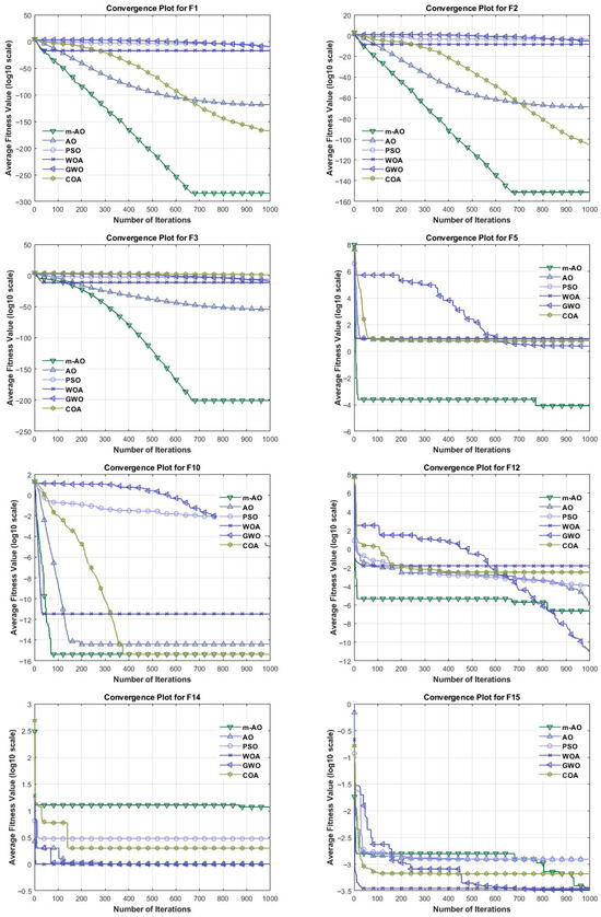
Furthermore, on test function C12, m-AO performs second-best. These outcomes show how well m-AO performs across the majority of test functions and how well the improvements made to the basic AO are. The convergence curves of the competing algorithm AO and m-AO on the CEC’22 test functions are shown in Figure 3. In comparison to other algorithms, m-AO exhibits faster convergence rates and higher accuracy in the early stages across all test functions. For original AO and proposed m-AO algorithm on the CEC’22 test functions, the convergence graph plots are shown in Figure 3.

Figure 3. The convergence trends of AO and m-AO on some CEC’22 functions.

5.5. Statistical Test

This section provides a statistical analysis of the simulation results, employing the Wilcoxon signed-rank test and the Friedman test to assess the differences in performance between m-AO and the other comparative algorithms [53].

5.5.1. Wilcoxon Signed Ranked Test

Table 7 and Table 8 present the outcomes of the Wilcoxon rank-sum test. The sums of ranks for positive and negative differences are denoted by $\sum R^{+}$ and $\sum R^{-}$, respectively. In most comparisons with other algorithms, m-AO exhibits a higher positive rank sum. The table also includes the corresponding z-scores and p-values, with a significance threshold set at α = 0.05. These results indicate that m-AO’s performance is statistically comparable to that of other metaheuristic algorithms [59,60].

Table 7. An overview of non-parametric statistical findings using the Bonferroni–Dunn and Wilcoxon tests.

Algorithms		ΣR+	ΣR−	z-Value	p-Value		Sign
m-AO vs	AO	38	17	1.070	0.285		+
	PSO	133	57	1.529	0.126		=
	WOA	134	97	0.643	0.520		+
	GWO	200	76	1.886	0.059		=
	COA	152	79	1.269	0.205		+
$\mathbf{CD} \mathbf{value} \mathbf{at} \alpha =0.1$	3.7432			CD value at  $\alpha =0.05$		3.8811

Table 8. An overview of non-parametric statistical findings using the Bonferroni–Dunn and Wilcoxon tests.

Algorithms		ΣR+	ΣR−	z-Value	p-Value		Sign
m-AO vs	AO	78	00	3.059	0.002		+
	COA	63	15	1.883	0.060		=
	PSO	78	00	3.059	0.002		+
	WOA	78	00	3.059	0.002		=
$\mathbf{CD} \mathbf{value} \mathbf{at} \alpha =0.1$	2.7546			CD value at  $\alpha =0.05$		2.9364

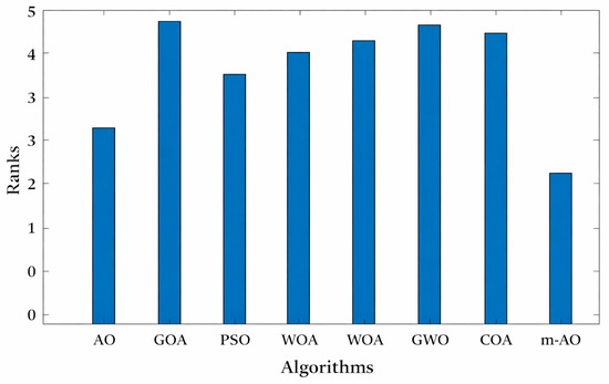
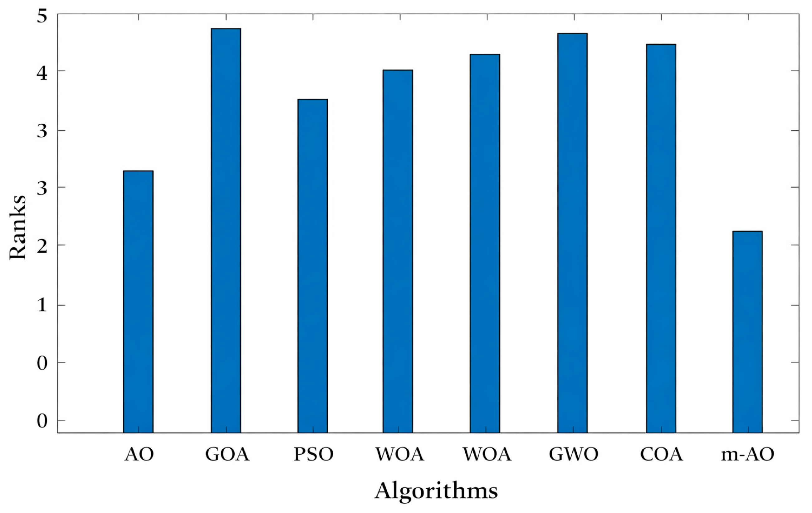
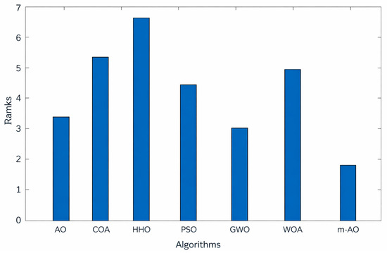
Additionally, the Bonferroni–Dunn test is applied to m-AO to detect significant performance differences, with findings reported in the final row of Table 7 and Table 8. Among the evaluated algorithms, m-AO achieves the lowest mean rank. This is further illustrated in the Bonferroni–Dunn graphic in Figure 4 and Figure 5, which depicts the rank variations for each method. In this figure, the algorithm with the shortest bar, representing the lowest rank, is identified as the best performer, while those with taller bars are considered to underperform relative to the control algorithm. The application of the Bonferroni–Dunn test confirms that m-AO performs favourably compared to other metaheuristic algorithms, with the SSA algorithm GOA, and HHO, respectively, exhibiting the weakest performance.

Figure 4. Dunn–Bonferroni test results of algorithms on Classical benchmark functions.

Figure 5. Dunn–Bonferroni test results of algorithms on CEC’22 benchmark functions.

Table 4 displays the simulation results of m-AO and its competitors for the Classical benchmark with 30 dimensions. Notably, none of the rival algorithms exhibit outstanding data in these Classical outcomes. For the CEC’22 benchmark with 10 dimensions, the results are presented in Table 5. m-AO demonstrates notable differences when compared to other algorithms. Although, it does not exhibit prominently highlighted data compared to the AO algorithm. To summarize, the analysis presented in Section 5.3 and Section 5.4 clearly indicates that m-AO outperforms various metaheuristic algorithms overall. This superior performance can be attributed to the effective strategies implemented in AO, including the adaptive chaotic reverse learning technique, the elite alternative pool technique, and the shifted distribution estimation technique. These findings emphasize m-AO’s competitive edge in tackling optimization problems across various benchmark functions.

5.5.2. Friedman Test

The m-AO algorithm’s performance on the Classical and CEC-2022 test sets was evaluated against other algorithms using the non-parametric Friedman average rank test [60]. The resulting rankings are displayed in Table 5 and Table 6. The analysis reveals that m-AO consistently achieves the top rank, demonstrating its superior performance compared to the benchmark algorithms across the examined test sets. Furthermore, the Friedman test results for classical and CEC-2022 indicate that m-AO secures the first position with a mean rank value of 2.46 for classical functions, followed by AO, PSO, WOA, COA, GWO, and GOA in ascending order and for CEC-2022 mean rank value of 1.33, followed by GWO, AO, PSO, WOA, COA, and HHO. These findings highlight the significant advantage of m-AO over other optimization algorithms.

5.6. Population Diversity Analysis

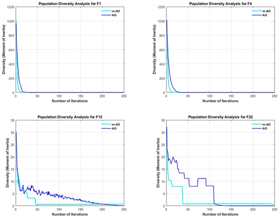
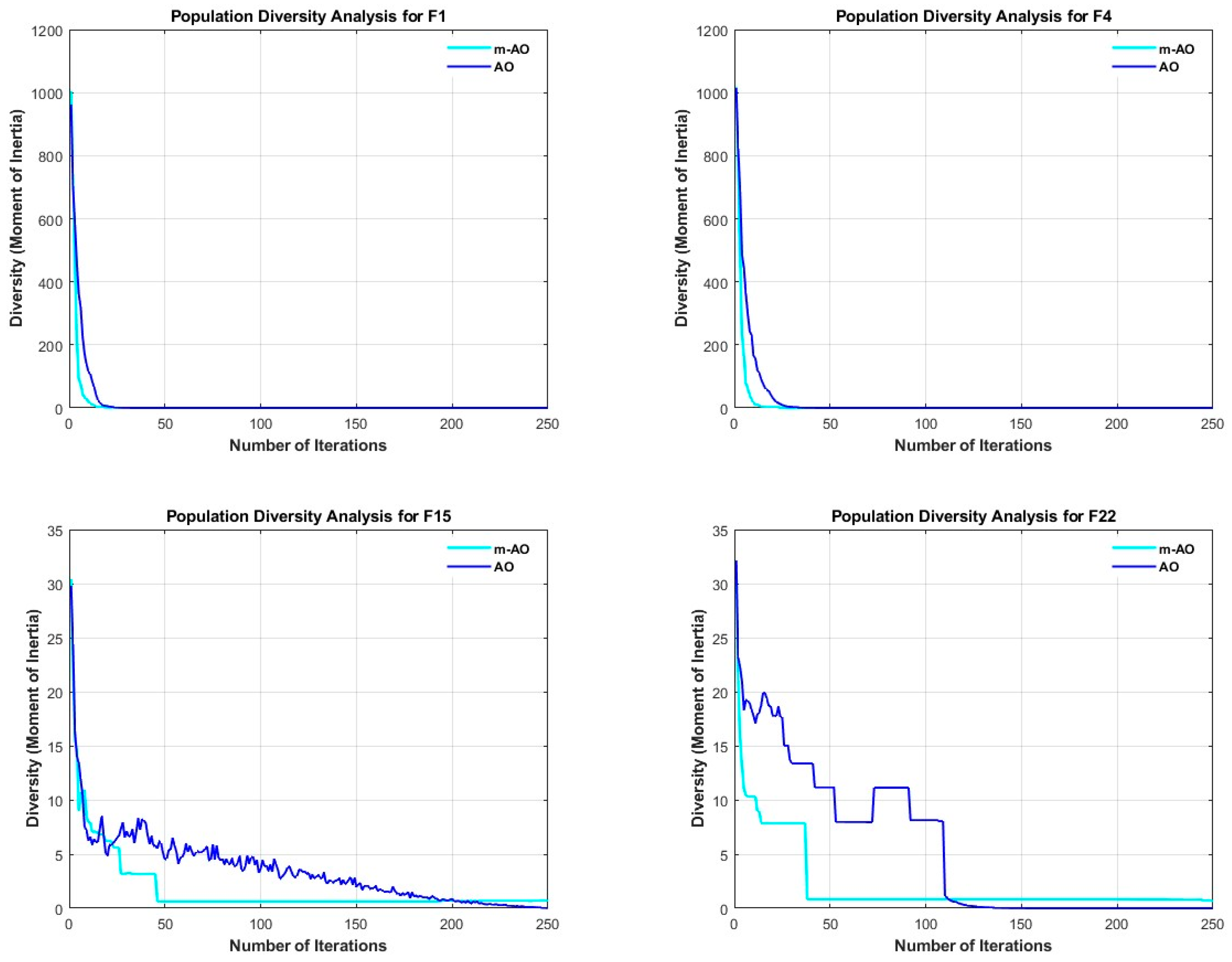
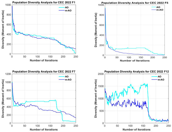
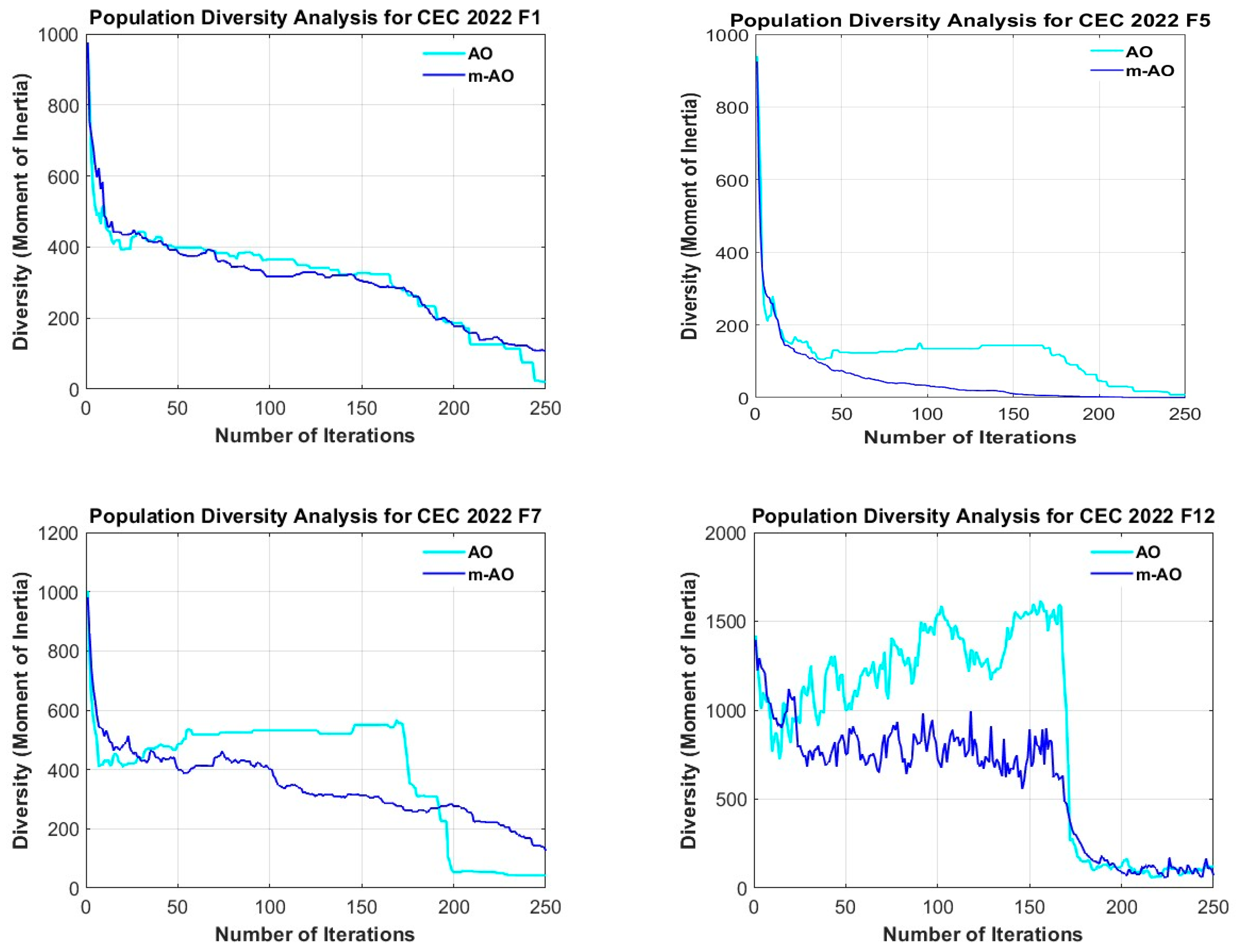
The diversity within a population significantly impacts the effectiveness of meta-heuristic algorithms. To examine the differences in population size between AO and m-AO, we performed population diversity experiments using the Classical suite and the CEC 2022 suite. In these tests, the moment of inertia, denoted as $I_C$, is employed to assess population diversity and evaluate algorithm performance, as expressed in Equation (32). The term $c_d$ reflects the spread between the population and the center of mass, c, in each iteration, and is computed using Equation (33). Here, $x_{id}$ represents the value of the dth dimension for the ith individual at iteration iter, while D signifies the total number of dimensions or variables in the problem.

$$I_C\left(iter\right)=\sqrt{\sum _{i=1}^{ps}\sum _{d=1}^D{\left(x_{id}\left(iter\right)-c_d\left(iter\right)\right)}^2}$$

(41)

$$c_d\left(iter\right)={\displaystyle \frac{1}{D}}\sum _{i=1}^{ps}{x}_{id}\left(iter\right)$$

(42)

As shown in Figure 6 and Figure 7, the simulation results indicate that m-AO demonstrates superior population diversity compared to AO in the early stages of the iteration process. This suggests that m-AO is capable of exploring the search space more comprehensively in the initial phase, effectively preventing premature convergence and local stagnation. In the later stages, the population diversity of m-AO falls below that of AO, indicating that m-AO transitions more rapidly from the exploration phase to the exploitation phase. This accelerates the convergence of the algorithm and reduces its computational cost. Therefore, m-AO algorithm has better performance.

Figure 6. Population diversity analysis of classical F1, F4, F15, and F22.

Figure 7. Population diversity analysis of CEC 2022 F1, F5, F7, and F12.

5.7. Exploration and Exploitation Analysis

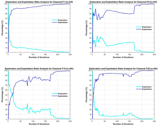
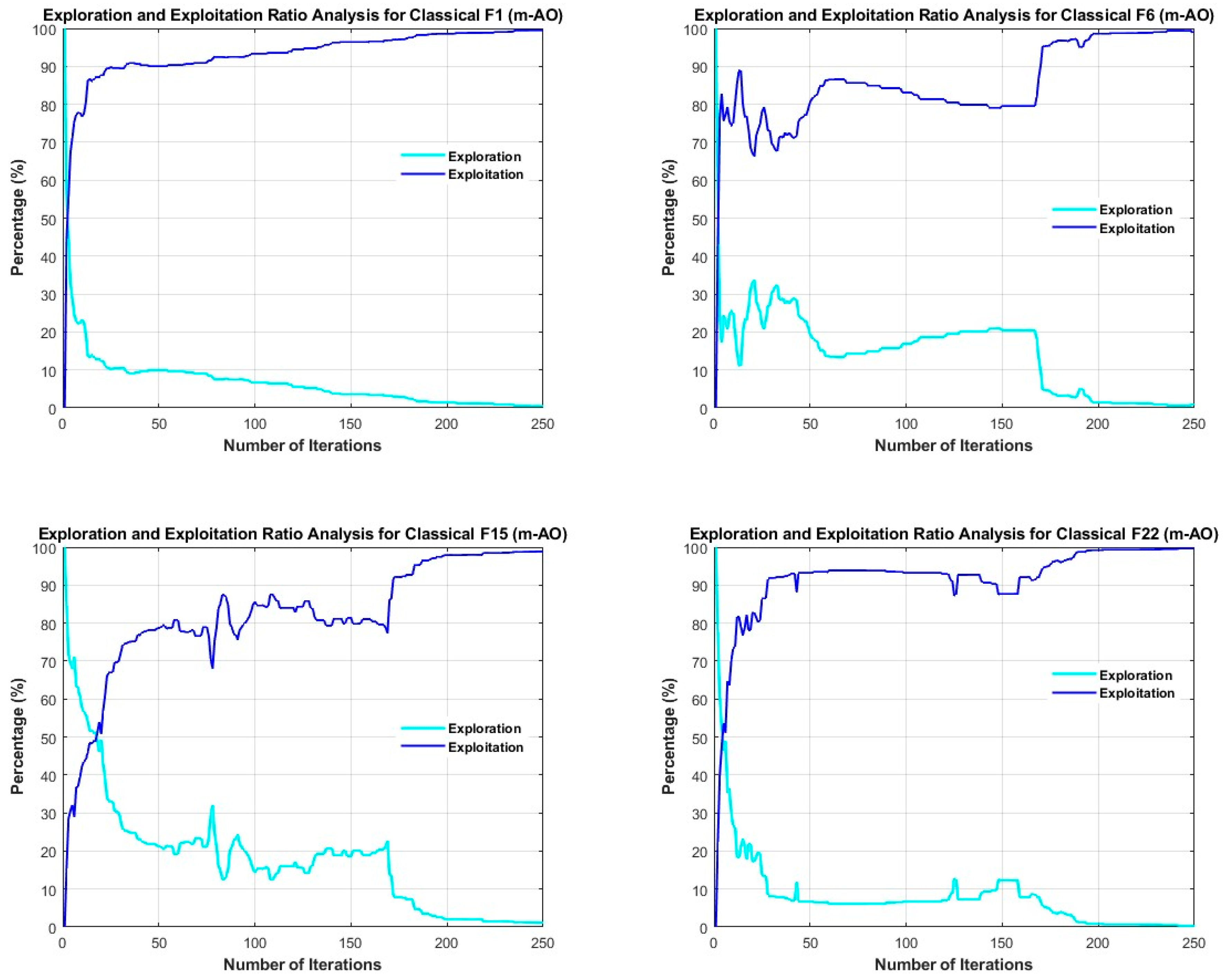
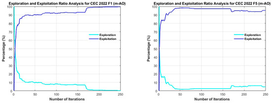
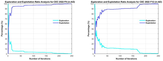
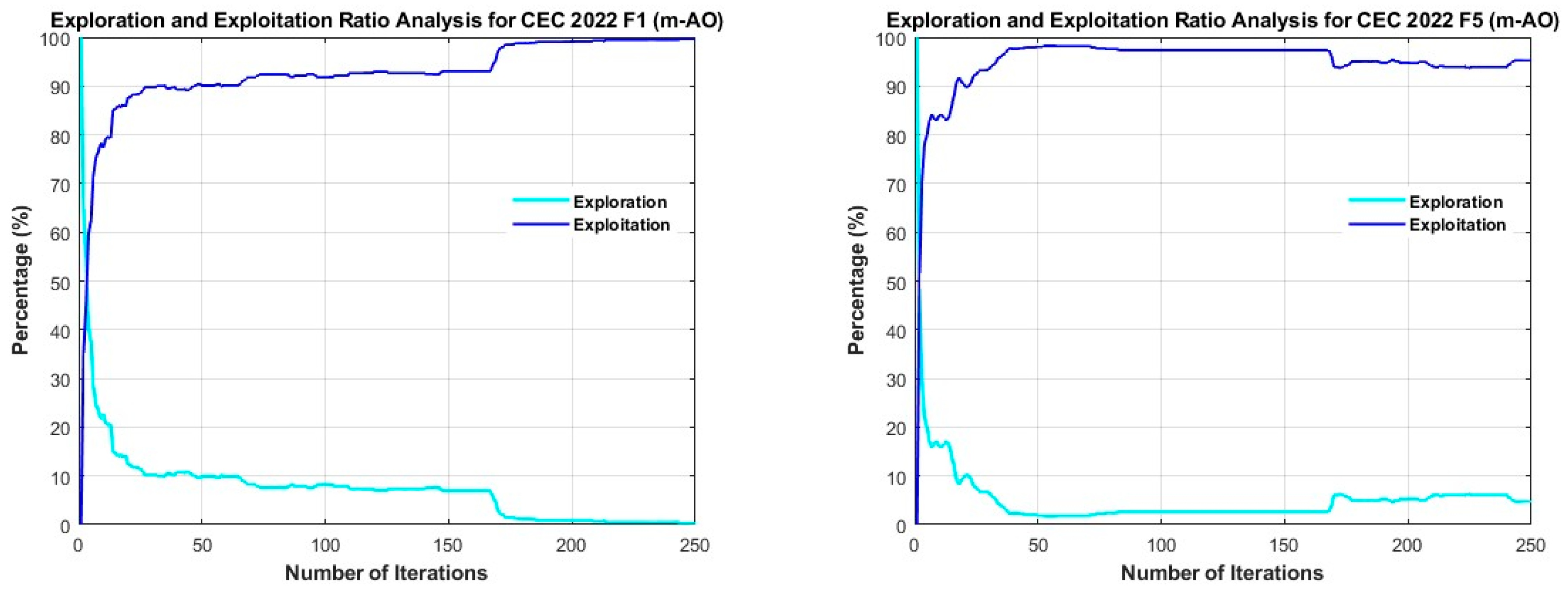
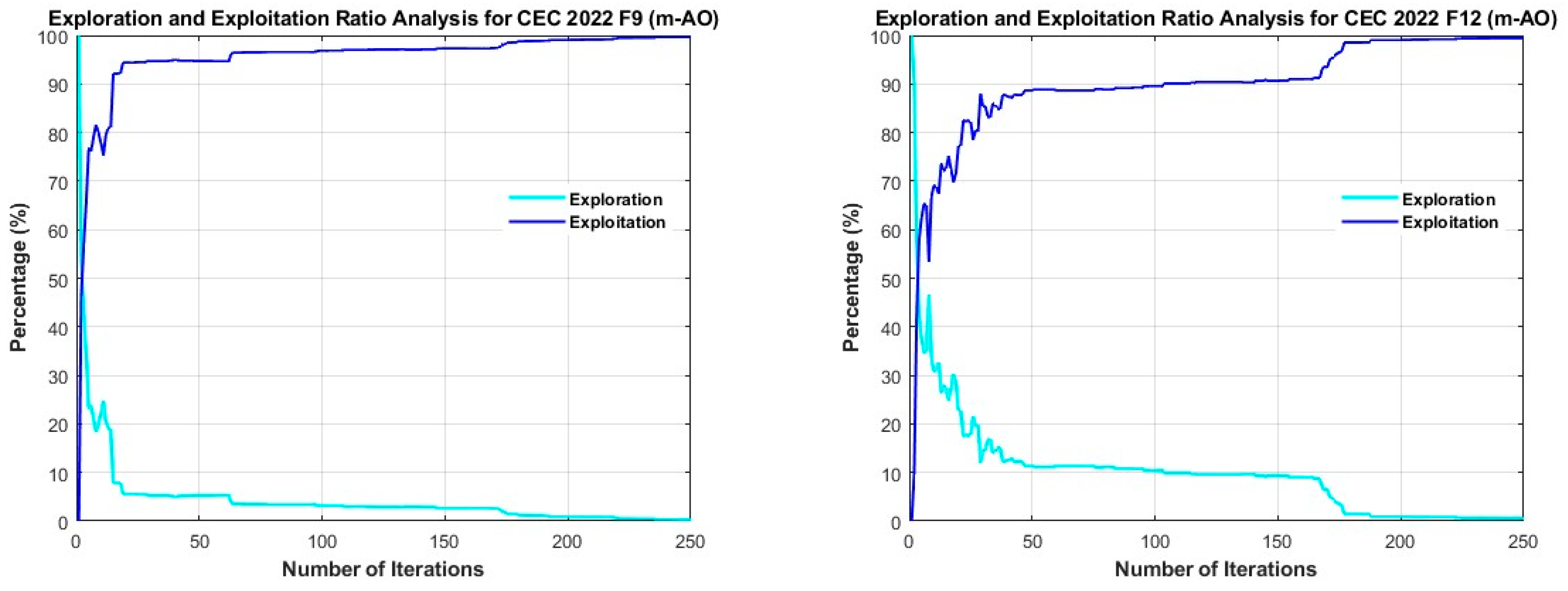
A fundamental feature of meta-heuristic algorithms lies in splitting the search process into two phases: exploration and exploitation. Achieving an effective balance between these phases is vital for enhancing algorithm performance. To assess this equilibrium, an experiment on exploration and exploitation employs percentage-based formulas, Equations (34) and (35). In these equations, the parameter $Di\nu \left(iter\right)$ quantifies dimensional diversity, determined through Equation (36), which reflects the expansion and contraction of distances among individuals in the population throughout the search. $Di{\nu }_{max}$ denotes the highest diversity observed across all iterations, while $x_{id}$ indicates the position of the ith individual in the d dimension. The percentage (%) expresses the degrees of exploration and exploitation across the entire population during the evolutionary process.

$$Exploration\left(\mathrm{\%}\right)={\displaystyle \frac{Di\nu \left(iter\right)}{Di{\nu }_{max}}}\times 100$$

(43)

$$Exploitation\left(\mathrm{\%}\right)={\displaystyle \frac{\left|Di\nu \left(iter\right)-Di{\nu }_{max}\right|}{Di{\nu }_{max}}}\times 100$$

(44)

$$Di\nu \left(iter\right)={\displaystyle \frac{1}{D}}{\sum }_{d=1}^D{\displaystyle \frac{1}{ps}}{\sum }_{i=1}^{ps}\left|median\left(x_d\left(iter\right)\hspace{0.25em}\right)-x_{id}\left(iter\right)\right|$$

(45)

The outcomes of the numerical simulations are depicted in Figure 8 and Figure 9, where the horizontal axis indicates the iteration count, and the vertical axis displays the percentage of exploration and exploitation across the population’s iterations. Initially, m-AO emphasizes exploration, reflected by a high percentage, indicating its ability to thoroughly investigate uncharted regions of the search space. As iterations advance, the share of exploitation rises, speeding up convergence and demonstrating the algorithm’s robust capacity for local optimization. Throughout this progression, m-AO sustains a flexible equilibrium between exploration and exploitation, which aids in preventing entrapment in local optima and avoids early convergence.

Figure 8. Exploration and exploitation analysis of classical benchmark functions F1, F6, F15, and F22.

Figure 9. Exploration and exploitation analysis of CEC 2022 benchmark functions F1, F5, F9, and F12.

5.8. m-AO on PFHE Design Problem

This section extends the optimization object to the PFHE design problem. Actually, the repeatability optimization problem and the PFHE design optimization challenge are not the same. Suboptimal plate–fin heat exchanger designs can lead to reduced heat transfer rates, excessive pressure losses, and unfavorable outlet temperatures, thereby increasing energy consumption and operational costs. Proper optimization enables improved thermal effectiveness, reduced hydraulic penalties, and enhanced overall system efficiency, which is critical in aerospace, cryogenic, and energy applications.

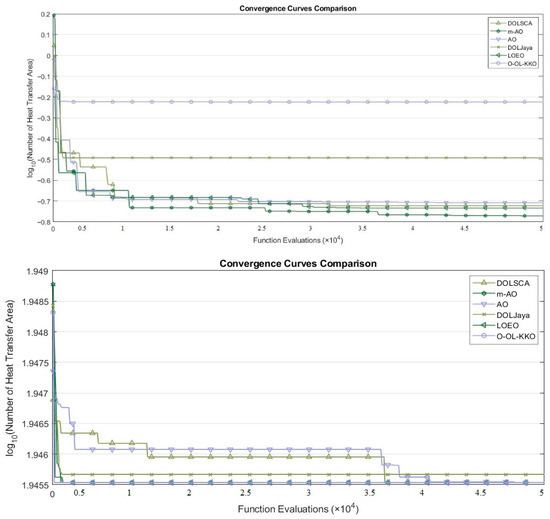
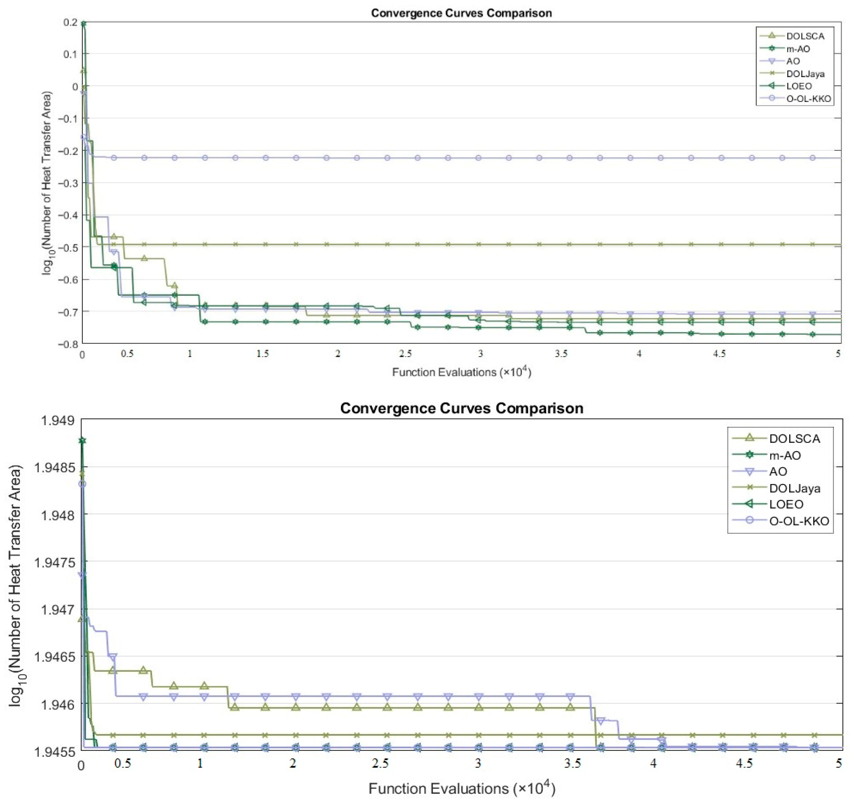
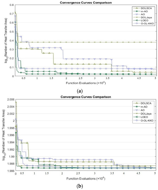
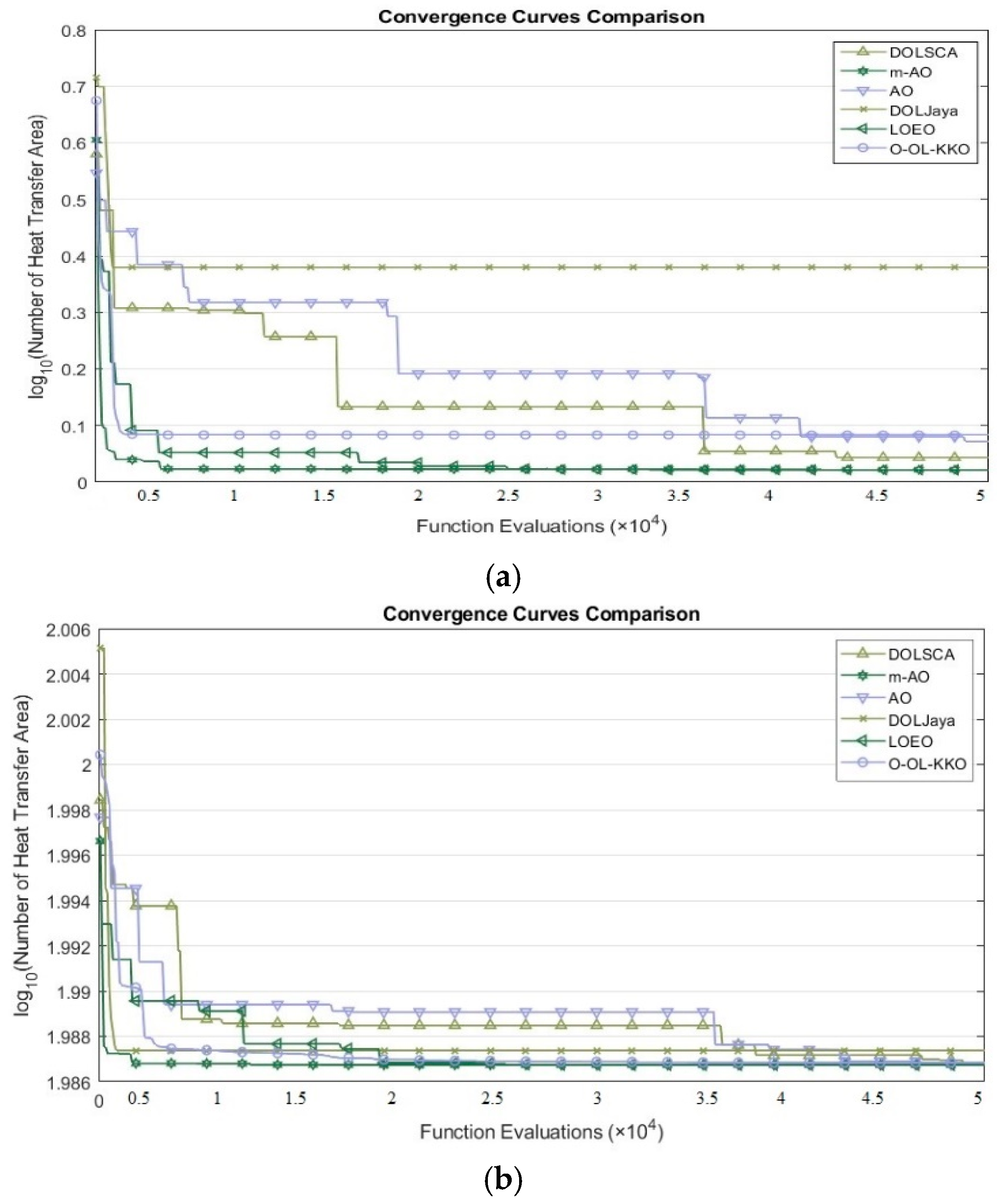
Only an optimal design is required for the design optimization problem; stability of the repeatability optimization is more crucial [61]. To maintain objectivity, the optimization process is executed ten times, and key performance metrics—including the best, worst, average, and standard deviation—are recorded for each case study and objective function combination. The average values from each iteration over the ten repetitions are plotted to depict the convergence trend. Since there are two design case studies and two objective functions—defined by Equation (20) (Objective Function 1) and Equation (21) (Objective Function 2)—a total of four result sets are analyzed. Additionally, the performance of five other optimization algorithms is included for comparison. The results are presented with the convergence trend for Objective Function 1 illustrated in Figure 10 and that for Objective Function 2 shown in Figure 11. In this part, we include the algorithms that are used to the application of PFHE design problems to compare the study’s fairness: DOLSCA (Dynamic Opposite learning enhanced Sine Cosine Algorithm) [62], DOLJaya (Dynamic Opposite learning enhanced Jaya Optimization) [63], LOEO (Levy-Opposition-Equilibrium Optimizer) [34], O-OL-KKO (Opposition-based Orthogonal Learning Kho-Kho Optimization) [64], and the base algorithm AO along with the modified Aquila Optimizer algorithm (m-AO). Figure 10 and Figure 11 present the findings.

Figure 10. Optimization results for the Ns objective (Case 1).

Figure 11. (a) Optimization results for the Case 1 AHT objective. (b) Optimization results for the Case 2 AHT objective.

The result image makes it clear that AO and m-AO are equally advantageous in terms of the AHT objective function. The enhanced method outperforms the original algorithm in terms of accuracy, and the m-AO maintained its convergence despite a large number of iterations. The accuracy difference is greater and m-AO converges more quickly than AO on the Ns objective function. At the same time, m-AO’s accuracy is the highest among the three situations, demonstrating its promise for engineering design optimisation issues. The outcomes of engineering and benchmark testing demonstrate that m-AO has outstanding overall performance, exceptional dynamic search capabilities, and distinct speed and accuracy benefits.

6. Conclusions and Future Works

This study presented a modified Aquila Optimizer (m-AO) aimed at overcoming the key limitations of the original AO, namely premature convergence, insufficient population diversity, and slow convergence behavior. Three complementary improvement strategies—adaptive chaotic reverse learning, elite alternative pooling, and shifted distribution estimation—were integrated into the AO framework to enhance global exploration while maintaining strong local exploitation.

The effectiveness of the proposed m-AO was rigorously verified through extensive numerical simulations involving 23 classical benchmark functions and the IEEE CEC 2022 test suite. The obtained results demonstrate that m-AO consistently achieves better or competitive optimal solutions with faster convergence rates compared to the original AO and other state-of-the-art metaheuristic algorithms. Statistical validation using Friedman ranking and Wilcoxon signed-rank tests further confirms the robustness and reliability of the proposed improvements.

Beyond benchmark validation, the practical applicability of m-AO was demonstrated through the optimal design of a plate–fin heat exchanger. The optimized designs obtained using m-AO show clear improvements in thermal–hydraulic performance, including reduced entropy generation and enhanced heat transfer effectiveness under prescribed constraints. These outcomes verify that the proposed algorithm is not only theoretically effective but also suitable for solving real-world engineering design problems characterized by strong nonlinearity and complex constraints.

The present thermo-hydraulic model neglects fouling resistance and axial heat conduction effects. These assumptions are commonly adopted in preliminary design-stage optimization; however, their inclusion may further refine long-term performance predictions and will be considered in future extensions of this work.

Overall, the proposed m-AO provides a flexible and efficient optimization framework with improved convergence accuracy and solution stability. Future research will focus on extending the proposed approach to multi-objective and constrained optimization scenarios, integrating surrogate or CFD-based models, and applying the method to other complex thermal and energy system optimization problems.

References

- Lincoln, G.A. Energy conservation. Science 1973, 180, 155–162. [Google Scholar] [CrossRef] [Scilit] [PubMed]
- Zhang, L.; Li, Y.; Zhang, H.; Xu, X.; Yang, Z.; Xu, W. A review of the potential of district heating system in northern China. Appl. Therm. Eng. 2021, 118, 116605. [Google Scholar] [CrossRef] [Scilit]
- Wu, Z.; Li, Q.; Wu, W.; Zhao, M. Crowdsourcing model for energy efficiency retrofit and mixed-integer equilibrium analysis. IEEE Trans. Ind. Inform. 2019, 16, 4512–4524. [Google Scholar] [CrossRef] [Scilit]
- Yang, Z.; Mourshed, M.; Liu, K.; Xu, X.; Feng, S. A novel competitive swarm optimized RBF neural network model for short term solar power generation forecasting. Neurocomputing 2020, 397, 415–421. [Google Scholar] [CrossRef] [Scilit]
- Wang, Z.; Li, Y. Layer pattern thermal design and optimization for multistream plate-fin heat exchangers—A review. Renew. Sustain. Energy Rev. 2016, 53, 500–514. [Google Scholar] [CrossRef] [Scilit]
- Van Laarhoven, P.J.; Aarts, E.H. Simulated annealing. In Simulated Annealing: Theory and Applications; Springer: Dordrecht, The Netherlands, 1987; pp. 7–15. [Google Scholar]
- Whitley, D. A genetic algorithm tutorial. Stat. Comput. 1994, 4, 65–85. [Google Scholar] [CrossRef] [Scilit]
- Kennedy, J.; Eberhart, R. Particle swarm optimization. In Proceedings of the ICNN’95-International Conference on Neural Networks, Perth, WA, Australia, 27 November–1 December 1995; IEEE: Piscataway, NJ, USA, 1995; Volume 4, pp. 1942–1948. [Google Scholar]
- Yang, X.-S.; Deb, S. Cuckoo search: Recent advances and applications. Neural Comput. Appl. 2014, 24, 169–174. [Google Scholar] [CrossRef] [Scilit]
- Mirjalili, S.; Mirjalili, S.M.; Lewis, A. Grey wolf optimizer. Adv. Eng. Softw. 2014, 69, 46–61. [Google Scholar] [CrossRef] [Scilit]
- Abeykoon, C. Compact heat exchangers-design and optimization with CFD. Int. J. Heat Mass Trans. 2020, 146, 118766. [Google Scholar] [CrossRef] [Scilit]
- Liu, C.; Bu, W.; Xu, D. Multi-objective shape optimization of a plate-fin heat exchanger using CFD and multi-objective genetic algorithm. Int. J. Heat Mass Trans. 2017, 111, 65–82. [Google Scholar] [CrossRef] [Scilit]
- Najafi, H.; Najafi, B. Multi-objective optimization of a plate and frame heat exchanger via genetic algorithm. Heat Mass Transf. 2010, 46, 639–647. [Google Scholar] [CrossRef] [Scilit]
- Rao, R.V.; Patel, V. Design optimization of shell and tube heat exchangers using swarm optimization algorithms. Proc. Inst. Mech. Eng. Part A J. Power Energy 2011, 225, 619–634. [Google Scholar] [CrossRef] [Scilit]
- Rao, R.V.; Saroj, A. Economic optimization of shell-and-tube heat exchanger using Jaya algorithm with maintenance consideration. Appl. Therm. Eng. 2017, 116, 473–487. [Google Scholar] [CrossRef] [Scilit]
- Iyer, V.H.; Mahesh, S.; Malpani, R.; Sapre, M.; Kulkarni, A.J. Adaptive range genetic algorithm: A hybrid optimization approach and its application in the design and economic optimization of shell-and-tube heat exchanger. Eng. Appl. Artif. Intell. 2019, 85, 444–461. [Google Scholar] [CrossRef] [Scilit]
- de Vasconcelos Segundo, E.H.; Mariani, V.C.; Coelho, L.d.S. Metaheuristic inspired on owls behavior applied to heat exchangers design. Therm. Sci. Eng. Prog. 2019, 14, 100431. [Google Scholar] [CrossRef] [Scilit]
- Rao, R.V.; Majethia, M. Design optimization of shell-and-tube heat exchanger using Rao algorithms and their variants. Therm. Sci. Eng. Prog. 2022, 36, 101520. [Google Scholar]
- Abualigah, L.; Yousri, D.; Abd Elaziz, M.; Ewees, A.A.; Al-Qaness, M.A.; Gandomi, A.H. Aquila optimizer: A novel meta-heuristic optimization algorithm. Comput. Ind. Eng. 2021, 157, 107250. [Google Scholar] [CrossRef] [Scilit]
- Fu, Y.; Liu, D.; Fu, S.; Chen, J.; He, L. Enhanced Aquila optimizer based on tent chaotic mapping and new rules. Sci. Rep. 2024, 14, 3013. [Google Scholar] [CrossRef] [Scilit]
- Gul, F.; Mir, I.; Mir, S. Aquila Optimizer with parallel computing strategy for efficient environment exploration. J. Ambient. Intell. Humaniz. Comput. 2023, 14, 4175–4190. [Google Scholar] [CrossRef] [Scilit]
- FatFatani, A.; Dahou, A.; Al-Qaness, M.A.A.; Lu, S.; Elaziz, M.A. Advanced feature extraction and selection approach using deep learning and Aquila optimizer for IoT intrusion detection system. Sensors 2021, 22, 140. [Google Scholar] [CrossRef] [Scilit]
- Zeng, L.; Li, M.; Shi, J.; Wang, S. Spiral aquila optimizer based on dynamic gaussian mutation: Applications in global optimization and engineering. Neural Process. Lett. 2023, 55, 11653–11699. [Google Scholar] [CrossRef] [Scilit]
- Mohamed, A.A.; Abualigah, L.; Alburaikan, A.; Khalifa, H.A.E.-W. AOEHO: A New Hybrid Data Replication Method in Fog Computing for IoT Application. Sensors 2023, 23, 2189. [Google Scholar] [CrossRef] [Scilit]
- Nirmalapriya, G.; Agalya, V.; Regunathan, R.; Ananth, M.B.J. Fractional Aquila spider monkey optimization based deep learning network for classification of brain tumor. Biomed. Signal Process. Control 2023, 79, 104017. [Google Scholar] [CrossRef] [Scilit]
- Varshney, M.; Kumar, P.; Ali, M.; Gulzar, Y. Dynamic Random Walk and Dynamic Opposition Learning for Improving Aquila Optimizer: Solving Constrained Engineering Design Problems. Biomimetics 2024, 9, 215. [Google Scholar] [CrossRef] [Scilit]
- Sasmal, B.; Hussien, A.G.; Das, A.; Dhal, K.G. A comprehensive survey on aquila optimizer. Arch. Comp. Methods Eng. 2023, 30, 4449–4476. [Google Scholar] [CrossRef] [Scilit]
- Wolpert, D.H.; Macready, W.G. No free lunch theorems for optimization. IEEE Trans. Evol. Comput. 1997, 1, 67–82. [Google Scholar] [CrossRef] [Scilit]
- Adam, S.P.; Alexandropoulos, S.A.N.; Pardalos, P.M.; Vrahatis, M.N. No free lunch theorem: A review. In Approximation and Optimization: Algorithms, Complexity and Applications; Springer: Cham, Switzerland, 2019; pp. 57–82. [Google Scholar]
- Adabbo, G.; Andreozzi, A.; Iasiello, M.; Napoli, G.; Vanoli, G.P. A multi-objective optimization framework through genetic algorithm for hyperthermia-mediated drug delivery. Comput. Biol. Med. 2025, 189, 10995. [Google Scholar]
- Vahideh, R.; Yaser, H.; Srikanth, R.; Cong, H.H.; Najmeh, F.; Charles, L.A.; Kamal, S.; Scott, N.S.; Bahgat, G.S. Multi-objective optimization of a chip-attached micro pin fin liquid cooling system. Appl. Therm. Eng. 2021, 195, 1171887. [Google Scholar]
- Khan, T.A.; Li, W. Optimal design of plate-fin heat exchanger by combining multi-objective algorithms. Int. J. Heat Mass Transf. 2017, 108, 1560–1572. [Google Scholar] [CrossRef] [Scilit]
- Peng, H.; Ling, X. Optimal design approach for the plate-fin heat exchangers using neural networks cooperated with genetic algorithms. Appl. Therm. Eng. 2008, 28, 642–650. [Google Scholar] [CrossRef] [Scilit]
- Rizk-Allah, R.M.; Hassanien, A.E.; Marafie, A. An improved equilibrium optimizer for numerical optimization: A case study on engineering design of the shell and tube heat exchanger. J. Eng. Res. 2024, 12, 240–255. [Google Scholar] [CrossRef] [Scilit]
- Yousefi, M.; Enayatifar, R.; Darus, A.N.; Abdullah, A.H. Optimization of plate-fin heat exchangers by an improved harmony search algorithm. Appl. Therm. Eng. 2013, 50, 877–885. [Google Scholar] [CrossRef] [Scilit]
- Incropera, F.P.; Lavine, A.S.; Bergman, T.L.; DeWitt, D.P. Fundamentals of Heat and Mass Transfer; Wiley: Hoboken, NJ, USA, 2007. [Google Scholar]
- Yousefi, M.; Darus, A.; Mohammadi, H. An imperialist competitive algorithm for optimal design of plate-fin heat exchangers. Int. J. Heat Mass Transf. 2012, 55, 3178–3185. [Google Scholar] [CrossRef] [Scilit]
- Joshi, H.M.; Webb, R.L. Heat transfer and friction in the offset strip fin heat exchanger. Int. J. Heat Mass Transf. 1987, 30, 69–84. [Google Scholar] [CrossRef] [Scilit]
- Bejan, A. Entropy Generation Minimization: The Method of Thermodynamic Optimization of Finite-Size Systems and Finite-Time Processes; CRC Press: Boca Raton, FL, USA, 2013. [Google Scholar]
- Guo, K.; Zhang, N.; Smith, R. Design optimisation of multi-stream plate fin heat exchangers with multiple fin types. Appl. Therm. Eng. 2018, 131, 30–40. [Google Scholar] [CrossRef] [Scilit]
- Reneaume, J.M.; Niclout, N. Plate fin heat exchanger design using simulated annealing. In Computer Aided Chemical Engineering; Elsevier: Amsterdam, The Netherlands, 2001; Volume 9, pp. 481–486. [Google Scholar]
- Tang, A.D.; Tang, S.Q.; Han, T.; Zhou, H.; Xie, L. A modified slime mould algorithm for global optimization. Comput. Intell. Neurosci. 2021, 2021, 2298215. [Google Scholar] [CrossRef] [Scilit] [PubMed]
- Zheng, T.; Luo, W. An enhanced lightning attachment procedure optimization with quasi-opposition based learning and dimensional search strategies. Comput. Intell. Neurosci. 2019, 2019, 1589303. [Google Scholar] [CrossRef] [Scilit]
- Wang, S.; Liu, Q.X.; Liu, Y.X.; Jia, H.; Abualigah, L.; Zheng, R.; Wu, D. A hybrid SSA and SMA with mutation opposition-based learning for constrained engineering problems. Comput. Intell. Neurosci. 2021, 2021, 6379469. [Google Scholar] [CrossRef] [Scilit]
- Yang, L.; Gao, S.C.; Yang, H.C.; Cai, Z.H.; Lei, Z.Y.; Todo, Y. Adaptive chaotic spherical evolution algorithm. Memetic Comput. 2021, 13, 383–411. [Google Scholar] [CrossRef] [Scilit]
- Geng, J.; Sun, X.; Wang, H.; Bu, X.; Liu, D.; Li, F.; Zhao, Z. A modified adaptive sparrow search algorithm based on chaotic reverse learning and spiral search for global optimization. Neural Comput. Appl. 2023, 35, 24603–24620. [Google Scholar] [CrossRef] [Scilit]
- Deng, L.; Liu, S. A sine cosine algorithm guided by elite pool strategy for global optimization. Appl. Soft Comput. 2024, 164, 111946. [Google Scholar] [CrossRef] [Scilit]
- Tang, A.; Zhou, H.; Han, T.; Xie, L. A modified manta ray foraging optimization for global optimization problems. IEEE Access 2021, 9, 128702–128721. [Google Scholar] [CrossRef] [Scilit]
- Wang, X.F.; Zhao, H.; Han, T.; Zhou, H.; Li, C. A grey wolf optimizer using Gaussian estimation of distribution and its application in the multi-UAV multi-target urban tracking problem. Appl. Soft Comput. 2019, 78, 240–260. [Google Scholar] [CrossRef] [Scilit]
- Ahrari, A.; Saadatmand, M.R.; Shariat-Panahi, M.; Atai, A.A. On the limitations of classical benchmark functions for evaluating robustness of evolutionary algorithms. Appl. Math. Comput. 2010, 215, 3222–3229. [Google Scholar] [CrossRef] [Scilit]
- Luo, W.; Lin, X.; Li, C.; Yang, S.; Shi, Y. Benchmark functions for CEC 2022 competition on seeking multiple optima in dynamic environments. arXiv 2022, arXiv:2201.00523. [Google Scholar] [CrossRef] [Scilit]
- Siegel, S. Nonparametric statistics. Am. Stat. 1957, 11, 13–19. [Google Scholar] [CrossRef] [Scilit]
- Nahm, F.S. Nonparametric statistical tests for the continuous data: The basic concept and the practical use. Korean J. Anesthesiol. 2016, 69, 8–14. [Google Scholar] [CrossRef] [Scilit]
- Meraihi, Y.; Gabis, A.B.; Mirjalili, S.; Ramdane-Cherif, A. Grasshopper optimization algorithm: Theory, variants, and applications. IEEE Access 2021, 9, 50001–50024. [Google Scholar] [CrossRef] [Scilit]
- Wang, D.; Tan, D.; Liu, L. Particle swarm optimization algorithm: An overview. Soft Comput. 2018, 22, 387–408. [Google Scholar] [CrossRef] [Scilit]
- Mirjalili, S.; Lewis, A. The whale optimization algorithm. Adv. Eng. Softw. 2016, 95, 51–67. [Google Scholar] [CrossRef] [Scilit]
- Jia, H.; Rao, H.; Wen, C.; Mirjalili, S. Crayfish optimization algorithm. Artif. Intell. Rev. 2023, 56, 1919–1979. [Google Scholar] [CrossRef] [Scilit]
- Heidari, A.A.; Mirjalili, S.; Faris, H.; Aljarah, I.; Mafarja, M.; Chen, H. Harris hawks optimization: Algorithm and applications. Future Gener. Comput. Syst. 2019, 97, 849–872. [Google Scholar] [CrossRef] [Scilit]
- Wilcoxon, F. Individual comparisons by ranking methods. Biom. Bull. 1945, 1, 80–83. [Google Scholar] [CrossRef] [Scilit]
- Derrac, J.; García, S.; Molina, D.; Herrera, F. A practical tutorial on the use of nonparametric statistical tests as a methodology for comparing evolutionary and swarm intelligence algorithms. Swarm Evol. Comput. 2011, 1, 3–18. [Google Scholar] [CrossRef] [Scilit]
- Yuen, S.Y.; Lou, Y.; Zhang, X. Selecting evolutionary algorithms for black box design optimization problems. Soft Comput. 2019, 23, 6511–6531. [Google Scholar] [CrossRef] [Scilit]
- Zhang, L.; Hu, T.; Yang, Z.; Yang, D.; Zhang, J. Elite and dynamic opposite learning enhanced sine cosine algorithm for application to plat-fin heat exchangers design problem. Neural Comput. Appl. 2023, 35, 12401–12414. [Google Scholar] [CrossRef] [Scilit]
- Zhang, L.; Hu, T.; Zhang, L.; Yang, Z.; McLoone, S.; Menhas, M.I.; Guo, Y. A novel dynamic opposite learning enhanced Jaya optimization method for high efficiency plate–fin heat exchanger design optimization. Eng. Appl. Artif. Intell. 2023, 119, 105778. [Google Scholar] [CrossRef] [Scilit]
- Mohapatra, S.; Das, D.K.; Singh, A.K. An optimal plate-fin heat exchanger design using opposition-based Orthogonal Learning Kho-Kho Optimization algorithm. Prog. Nucl. Energy 2024, 177, 105416. [Google Scholar] [CrossRef] [Scilit]
Disclaimer/Publisher’s Note: The statements, opinions and data contained in all publications are solely those of the individual author(s) and contributor(s) and not of MDPI and/or the editor(s). MDPI and/or the editor(s) disclaim responsibility for any injury to people or property resulting from any ideas, methods, instructions or products referred to in the content. |
© 2026 by the authors. Licensee MDPI, Basel, Switzerland. This article is an open access article distributed under the terms and conditions of the Creative Commons Attribution (CC BY) license.