Disclosing Information About the Asset Value Range in Market

Abstract

The information released to investors in financial markets takes various forms. We understand range information as information about the upper and lower bounds that the payoff of a risky asset may reach in the future. This study develops rational expectation models to explore the market impacts of disclosing such information. Our model shows that its disclosure can decrease market price sensitivity to private signal and increase market liquidity. Furthermore, the market impact of its disclosure depends on the position and precision of the range disclosed. When the linear combination of private signal and noise trading volume is distant from the disclosed range, the reaction of price to a variation in private signal will almost vanish, whereas movement in the disclosed range can efficiently impact price. Under certain conditions, such as a high proportion of informed traders or a small size of noise trading in the market, disclosing range information is more likely to reduce asset price and raise capital cost.

1. Introduction

In the financial market, the completeness of information known by different investors varies; this is known as information asymmetry. Disclosing information to market investors has a significant impact on market operation. A large number of studies specifically focus on the impact of information distribution on market price formation, as well as prices’ sensitivity to the information released and market quality. The latter mainly includes market liquidity, price volatility, market efficiency, etc.

A significant portion of the theoretical research on this topic has been developed under the framework of rational expectation. This series of studies assumes that traders with less information can use market prices to infer the private information known by traders who are more informed and apply their inference outcomes to make investment decisions.

Grossman and Stiglitz (1980) [1] conducted an early study based on the rational expectation framework. In their setup, there are both informed and uninformed traders in the market. Informed traders can obtain a private signal about asset value, while uninformed traders can only observe asset price and then infer private signals from informed traders accordingly. Under this setup, Grossman and Stiglitz (1980) [1] analyzed the trading behavior of the two trader types and market equilibrium.

In recent years, research on this topic has focused more on investors’ acquisition and processing of information, as well as the impact of their behaviors in these regards on market prices and quality. Furthermore, based on the rational expectation model framework, this series of literature argues that investors’ information learning and processing can be more complex in some situations, in turn changing their trading behavior. These situations mainly include the following:

(1)

Investors face ambiguity about some asset market parameters.

(2)

Asset value is composed of multiple fundamentals.

(3)

There is a deviation in investors’ interpretation of information in the market.

The first strand of the literature is developed under the assumption that some investors’ beliefs about some key parameters are ambiguous, making it more complicated for them to confirm the optimal trading volume. For example, Epstein and Schneider (2008) [2] discussed markets where some investors have such ambiguity in their perception of signal accuracy. Mele and Sangiorgi (2015) [3], Hahn and Kwon (2015) [4], Condie and Ganguli (2017) [5], and Huo et al. (2024) [6] focused on markets where ambiguity arises in some investors’ beliefs about the unconditional asset value mean. Easley et al. (2014) [7], Huang et al. (2017) [8], and Illeditsch et al. (2021) [9] considered markets where some investors experience ambiguity regarding the correlation coefficient between different asset values. Anthropelos and Schneider (2024) [10] and Ghazi et al. (2025) [11] introduce the scenario of investor belief ambiguity in asset payoff distribution. These studies show that ambiguity on the part of investors can lead to significant changes in their trading behavior, the market price, and quality.

The second strand of the literature analyzes markets where asset value is determined by multiple fundamentals and where different groups of informed traders can obtain private signal about different fundamentals; examples of studies on this topic include Kondor (2012) [12], Goldstein and Yang (2015) [13], Liu et al. (2019) [14], and Yang and Zhu (2020) [15]. When various traders transact, information about multiple fundamentals is injected into the market price simultaneously. In a complicated way, these fundamentals are then reflected in the asset price, which can make it more difficult for uninformed traders to infer information about asset fundamentals from the price, reducing inference result accuracy. The above literature shows that investor trading behavior, market price, and quality are distinct when setting up multiple fundamentals.

The third strand of the literature is developed under the assumption that there is a deviation in some investors’ interpretation of signals about asset value, which can make their trading decision deviate from the optimal. Authors in this field, such as Dumas et al. (2017) [16], Banerjee et al. (2018) [17], Liu et al. (2021) [18], and Hu and Wang (2024) [19], analyze how equilibrium price and market quality would be affected by such deviations.

Existing studies usually depict the information acquired by investors in two similar ways. Suppose a risky asset has an uncertain future value $v$. Based on the assumption that $v$ consists of several parts, such as $v=v_1+v_2$, the first way is to take the realized value of $v_1$ or $v_2$ as the information acquired by investors.

Use $\eta$ to represent a stochastic error item. The second way is to take the realized value of $v+\eta$ as the information acquired by investors.

The two ways of depicting information are essentially the same and we refer to them as common-form signals. To reflect market information asymmetry, related studies usually assume that informed traders can receive these signals while uninformed traders cannot, or the former can receive more signals than the latter.

However, there are several forms of market information that investors can obtain. Some information may reflect the upper or lower bounds that the future value of asset may reach. We refer to this type of information as range information about asset value.

Many countries have a price limit regime in their security markets. For example, the Shanghai and Shenzhen stock exchange imposes a price limit of 10% on the trading of main board stocks (see [20,21]). If some investors need to sell the stocks they hold before a certain future date, the trading price cannot exceed a specific level under this regime. This level then becomes the upper bound of their stock value. Since the magnitude of the limits on stock price fluctuations is uniformly set by the government, the upper and lower bounds of stock prices can be viewed as exogenous and all investors trading in the main board market are subject to these regulatory price limits.

Additionally, security analysts are often keen to make predictions about the upper or lower bounds of future asset value, and their predictions can possibly convince investors.

In some cases, a public company or some financial institutions may need to prevent their stock price from falling below a certain level; to achieve this, they can take some powerful measures. For example, some countries, such as the U.S., allow public companies to provide their shareholders with stock repurchase at an offer price (see [22]). Many repurchase programs are open to all shareholders, and every shareholder can participate in the buyback. In tender offer repurchases, the offer price is deliberately set by the company. If the shareholders acquire information regarding a company’s repurchase plan, they may believe they can sell their stocks at a price that is no lower than the offer price, leading this price to become the lower bound of their stock value.

Similarly, some block-holders may sell their shares in large quantities to realize profits when the stock price rises to a certain, previously set level, which can prevent the price from rising further. Once investors acquire the above insider information, they will also form beliefs about the upper bound of the future stock value.

In summary, public companies, financial institutions, security analysts, block-holders, or governments may intervene in the transaction price of asset, which can cause prices to have lower or upper bounds and limit their future value in a range. In reality, information about the series of interventions should be regarded as range information, some of which can be disclosed to the public.

Thus, range information is likely to exist in investors’ information set and affect their belief. The main issue we want to explore is the impact of disclosing range information on investor trading behavior, market price formation, and market quality.

Existing theoretical research has not yet studied range information nor introduced it into market micro-structure models. By introducing such information into rational expectation models, this study reveals how its disclosure can significantly change investor behavior, market equilibrium, and market quality compared with the existing theoretical literature. More specifically, we reveal whether market price and quality (such as liquidity and asset premium) will increase or decrease after range information is disclosed to investors, and how market price reacts to variation in private signal and the disclosed range. For example, we find that its disclosure can cause market liquidity, with the market price’s reaction to private signals varying continuously with private signal and noise trading volume. In models in the related literature, market liquidity and price reactions are usually constant—or piecewise constant—with private signal and noise trading. As such, we reveal that disclosure can lead to a new market price pattern in response to private signal and noise trading, along with a new market liquidity pattern, something which has rarely been recorded in the existing literature.

In Grossman and Stiglitz’s model (1980) [1], all investors explicitly know the asset value probability distribution. The first strand of the related literature introduces ambiguity into some investors’ perception of distribution parameters. As such, they do not explicitly know the distribution of asset value or signal, only that it belongs to a parametric distribution family, implying that the introduction of ambiguity weakens these investors’ information sets. Table 1 gives some comparisons between our model with range information and existing models with ambiguity. The second strand of the related literature introduces multiple fundamentals into asset value composition. Under this setup, the asset value is composed of several mutually independent fundamentals, but none of their realized values can be acquired by uninformed traders. The introduction of multiple fundamentals thus also weakens these investors’ information sets. The third strand of the related literature introduces deviation into some investors’ interpretation of asset value signals. This results in a bias in the information acquired relative to the actual signal, which also, again, weakens their information set. However, disclosing range information would increase the information acquired by investors, who then must make decisions based on more types of information. Thus, in contrast to existing studies, investor information sets are strengthened in our model.

Table 1. Main distinctions between existing models with ambiguity and our model with range information.

Dimensions for Comparison	Existing Models with Ambiguity	Our Model with Range Information
Information structure	The distribution of asset value or signal is ambiguous for some investors.	The distribution of asset value or signal is explicit for all investors; however, the distribution of asset value is truncated.
Belief update	Uninformed investors have to update their belief with a less informative signal extracted from price.	Uninformed investors can update their belief with a signal extracted from price, with no reduction in its informativeness.
Equilibrium price analysis	The reaction of equilibrium price to private signal is constant or piecewise constant.	The reaction of equilibrium price to private signal varies continuously.

The remainder of this paper is organized as follows. Section 2 presents our main model; with this, we analyze the trading behavior of various investors and the market equilibrium when range information is disclosed to investors. In Section 3, we use a benchmark model to present the trading behavior of various traders and market equilibrium in a situation where range information is not disclosed. Section 4 analyzes market price, price’s reaction to variation in private signal and the disclosed range, market liquidity, and the asset premium in the equilibrium of our main model. We then compare the equilibriums of the two models to reveal the impact of range information disclosure. Finally, Section 5 concludes our study.

2. The Main Model

2.1. Setup

Following Mondria et al. (2022) [23] and Huang et al. (2020) [24], we assume that the asset market is perfectly competitive and lasts for three periods: t = 0, 1 and 2.

There are two assets traded in the market. The first is a risk-free bond with unlimited supply. Following Easley et al. (2014) [7] and Mondria et al. (2022) [23], we also suppose, for simplicity, that its price is always 1 during these three periods. The second asset is the stock of a public company, with a total supply of $Z$ units, and it should be regarded as a risky asset.

Use $v$ to denote the payoff on one unit of risky asset. At t = 0, $v$ is uncertain for all investors and can be regarded as the future value of the risky asset, which means nobody knows the realized value of $v$. As time goes by, the realized value of $v$ is revealed and observable to all investors at t = 1. At t = 2, the risky asset pays off its holders, and a holder of each unit can obtain an amount of $v$.

Investors are all short-term traders and exist in the market for only two periods. More concretely, the first generation of investors trade at t = 0 and have to sell their assets in the market to obtain cash for their consumption at t = 1. Similarly, the second generation of investors trade at t = 1 and obtain asset payoffs at t = 2.

Following Grossman and Stiglitz (1980) [1] and Huang et al. (2020) [24], we assume that

$$v=u+\epsilon ,$$

where $u~N({\mu }_0,{\sigma }_u^2)$ and $\epsilon ~N(0,{\sigma }_{\epsilon }^2)$; $u$ and $\epsilon$ are mutually independent; $u$ can be regarded as the fundamental of the company, and $\epsilon$ can be referred to as the disturbance of some unobservable random factors on its future value.

At t = 0, investors can finance their purchase of risky assets by selling risk-free bonds short, with no restrictions on the amount of short selling.

Following Goldstein and Yang (2017) [25], there are three types of investors in the market: informed, uninformed, and noise traders. Suppose the fraction of informed traders and uniformed traders are respectively $x_I$ and $x_U$ with $x_I+x_U=1$.

Noise traders totally demand $y$ units of the risky asset at t = 0, that is, $y$ is noise trading volume. $y~N(0,{\sigma }_y^2)$ and $y$ is independent of $u$ and $\epsilon$. A larger ${\sigma }_y^2$ implies a greater size of noise trading in the market. In the following, we use $\tilde{y}$ to denote the realized value of $y$.

At t = 0, informed traders can observe the realized value of $u$, while uninformed traders cannot, which implies $u$ can be regarded as informed traders’ private signal about $v$. A larger variance value ${\sigma }_u^2$ implies a greater informativeness of the private signal. $\epsilon$ is unobservable to all investors and can be treated as the error of informed traders’ private signal $u$. Given that $Var\left[v|u\right]={\sigma }_{\epsilon }^2$, a smaller value of its variance ${\sigma }_{\epsilon }^2$ implies a smaller deviation of $u$ from the asset future value $v$ and then a more precise signal received by informed traders.

The related literature typically assumes that uninformed traders are aware that informed traders’ information is more sufficient than theirs (see, for example, Goldstein and Yang (2015) [13] and Easley and O’Hara (2009) [26]). We adhere to this assumption by supposing that uninformed traders perceive that informed traders can receive a private signal $u$ while they cannot.

Next, we introduce range information about risky asset value at t = 1 into our setup as follows.

There is a price limit regime in the market, and, under this regime, the stock cannot be traded at a price lower than ${\underset{\_}{v}}_{ r}$ or higher than ${\overline{v}}_r$ at t = 1. In addition, the management of the public company needs to keep its stock price above a certain level for certain reasons, such as to ensure the stability of their positions or prevent the company from being delisted. Then, in order to boost market confidence, the company at t = 0 promises to provide its shareholders with a stock repurchase offer at t = 1 with an offer price of ${\underset{\_}{v}}_{ c}$, where ${\underset{\_}{v}}_{ c}>{\underset{\_}{v}}_{ r}$ and ${\underset{\_}{v}}_{ c}<{\overline{v}}_r$.

Suppose that the range information above is disclosed to all investors at t = 0. For the first generation of investors, if the payoff $v$ revealed at t = 1 is between ${\underset{\_}{v}}_{ c}$ and ${\overline{v}}_r$, then they can sell their stocks at a price of $v$ given the full competitiveness of the market. If $v$ revealed at t = 1 is higher than ${\overline{v}}_r$, then they still have to sell their stocks at a price of ${\overline{v}}_r$ for their consumption. If $v$ revealed at t = 1 is lower than ${\underset{\_}{v}}_{ c}$, then they would accept the repurchase offer and sell their stocks to the company at a price of ${\underset{\_}{v}}_{ c}$ per share.

As a result, disclosing the range information at t = 0 suggests that the upper and lower bounds of the risky asset value at t = 1 are, respectively, ${\overline{v}}_r$ and ${\underset{\_}{v}}_{ c}$, that is, $v\in \left[\underset{\_}{v} , \overline{v}\right]$, where $\underset{\_}{v}={\underset{\_}{v}}_{ c}$ and $\overline{v}={\overline{v}}_r$.

Before trading, every investor is endowed with $D_0$ units of the risk-free bond.

At t = 0, the price of the risky asset is denoted by $p$. Use ${\mathrm{\theta }}_I$ and ${\mathrm{\theta }}_U$, respectively, to denote informed and uninformed traders’ demand for risky assets. Then, their wealths at t = 1 are, respectively,

$$W_I=D_0+{\mathrm{\theta }}_I(v-p)$$

and

$$W_U=D_0+{\mathrm{\theta }}_U\left(v-p\right).$$

Suppose that all the investors have a CARA utility function with a common absolute risk aversion coefficient $\gamma$, that is,

$$U\left(W\right)=-e^{-\gamma ·W},$$

where $W$ is the wealth held by the investor at t = 1. At t = 0, every investor trades in order to maximize the expectation of his utility conditional on his information set.

Under our assumptions, the market clearing condition should be

$$x_I{\theta }_I+x_U{\theta }_U+\tilde{y}=Z.$$

(1)

2.2. Informed Traders’ Decisions

Consider a representative informed trader. The realized value of $u$ is denoted by $\tilde{u}$, and their information set is $\left\{u=\tilde{u}, v\in \left[\underset{\_}{v} , \overline{v}\right] \right\}$. The conditional expectation of their utility is

$$U_I\left({\mathrm{\theta }}_I\right)\triangleq E\left[-e^{-\gamma \left(D_0+{\mathrm{\theta }}_I\left(v-p\right)\right)}\left|u=\tilde{u}, v\in \left[\underset{\_}{v} , \overline{v}\right] \right.\right].$$

Their decision problem is

$$\underset{{\theta }_I}{\max } U_I\left({\mathrm{\theta }}_I\right).$$

Use $\mathsf{\Psi }(·)$ and $\psi (·)$ to denote the cumulative distribution and probability density function of the standard normal distribution, respectively. We can derive

$$\begin{array}{ll}& U_I\left({\mathrm{\theta }}_I\right)\\ =& {\displaystyle \frac{E\left[-e^{-\gamma \left(D_0+{\mathrm{\theta }}_I\left(v-p\right)\right)}{{\displaystyle 1}}_{\left\{v\in \left[\underset{\_}{v} , \overline{v}\right]\right\}}\left|u=\tilde{u}\right.\right]}{E\left[{{\displaystyle 1}}_{\left\{v\in \left[\underset{\_}{v} , \overline{v}\right]\right\}}\left|u=\tilde{u}\right.\right]}}\\ =& -e^{-\gamma D_0+\gamma \left(p-\tilde{u}\right){\mathrm{\theta }}_I+{\displaystyle \frac{{\gamma }^2{\sigma }_{\epsilon }^2{\theta }_I^2}{2}}}· {\displaystyle \frac{\mathsf{\Psi }\left(\frac{\overline{v}+\gamma {\sigma }_{\epsilon }^2{\mathrm{\theta }}_I-\tilde{u}}{{\sigma }_{\epsilon }}\right)-\mathsf{\Psi }\left(\frac{\underset{\_}{v}+\gamma {\sigma }_{\epsilon }^2{\mathrm{\theta }}_I-\tilde{u}}{{\sigma }_{\epsilon }}\right)}{\mathsf{\Psi }\left(\frac{\overline{v}-\tilde{u}}{{\sigma }_{\epsilon }}\right)-\mathsf{\Psi }\left(\frac{\underset{\_}{v}-\tilde{u}}{{\sigma }_{\epsilon }}\right)}}.\end{array}$$

(2)

where ${{\displaystyle 1}}_{\left\{v\in \left[\underset{\_}{v} , \overline{v}\right]\right\}}$ is an indicator function.

We provide details about the calculation of Equation (2) in Appendix A.1. The derivative of the utility with respect to ${\mathrm{\theta }}_I$ is

$$U_I^{\prime }\left({\mathrm{\theta }}_I\right)=-\gamma ·U_I\left({\mathrm{\theta }}_I\right)·\left[{\mathit{J}}_{\left[ \underset{\_}{v} ,\overline{v} \right]}\left(\tilde{u}-\gamma {\sigma }_{\epsilon }^2{\mathrm{\theta }}_I\right)-p\right],$$

(3)

where ${\mathit{J}}_{\left[ \underset{\_}{v} ,\overline{v} \right]}\left(t\right)\triangleq {\sigma }_{\epsilon }\left[{\displaystyle \frac{\psi \left(\frac{\underset{\_}{v}-t}{{\sigma }_{\epsilon }}\right)-\psi \left(\frac{\overline{v}-t}{{\sigma }_{\epsilon }}\right)}{\mathsf{\Psi }\left(\frac{\overline{v}-t}{{\sigma }_{\epsilon }}\right)-\mathsf{\Psi }\left(\frac{\underset{\_}{v}-t}{{\sigma }_{\epsilon }}\right)}}\right]+t$.

We give a closed-form solution of an informed trader’s optimal decision as follows. The proof is given in Appendix A.3.

Proposition 1. 

For a given price$p\in ( \underset{\_}{v} , \overline{v})$, an informed trader’s optimal demand for the risky asset is $\widetilde{{\mathrm{\theta }}_I}={\displaystyle \frac{1}{\gamma {\sigma }_{\epsilon }^2}}·\tilde{u}+k$, where the parameter $k$ is the solution of

$$p={\mathit{J}}_{\left[ \underset{\_}{v} ,\overline{v} \right]}\left(-\gamma {\sigma }_{\epsilon }^{2}k\right).$$

(4)

The equation above has a unique solution.$\widetilde{{\theta }_I}$decreases monotonically with the price$p$. For a given price$p\le \underset{\_}{v} \mathit{and} p\ge \overline{v}$, the optimal demands are, respectively, positive infinity and negative infinity.

According to Item (3) of Appendix A.2, we have ${\mathit{J}}_{\left[ \underset{\_}{v} ,\overline{v} \right]}\prime \left(t\right)>0$, which implies ${\mathit{J}}_{\left[ \underset{\_}{v} ,\overline{v} \right]}\left(t\right)$ is continuous and increases monotonically with $t$. As such, it must have an inverse function ${\mathit{J}}_{\left[ \underset{\_}{v} ,\overline{v} \right]}^{-1}(·)$. Proposition 1 actually shows that the optimal demand is

$$\widetilde{{\theta }_I}={\displaystyle \frac{1}{\gamma {\sigma }_{\epsilon }^2}}·\tilde{u}-{\displaystyle \frac{{\mathit{J}}_{\left[ \underset{\_}{v} ,\overline{v} \right]}^{-1}\left(p\right) }{\gamma {\sigma }_{\epsilon }^2}},$$

which implies that $\widetilde{{\theta }_I}$ includes two parts. The first part ${\displaystyle \frac{1}{\gamma {\sigma }_{\epsilon }^2}}·\tilde{u}$ depends on the private signal $\tilde{u}$ and is independent of the range information (i.e., the lower bound $\underset{\_}{v}$ and the upper bound $\overline{v}$) and the price $p$. On the contrary, the second part $-{\displaystyle \frac{{\mathit{J}}_{\left[ \underset{\_}{v} ,\overline{v} \right]}^{-1}\left(p\right) }{\gamma {\sigma }_{\epsilon }^2}}$ depends on the range information and the price $p$, but cannot be affected by the private signal $\tilde{u}$.

Proposition 1 confirms that the market cannot reach equilibrium at a price $p\notin (\underset{\_}{v}, \overline{v})$. If it reaches equilibrium at a price $p\le \underset{\_}{v}$ ($\ge \overline{v}$), the demand of an informed trader is $\widetilde{{\mathrm{\theta }}_I}=+\infty$ ($-\infty$). Since $\widetilde{{\mathrm{\theta }}_I}\notin R$, this market state should not be considered as an equilibrium according to the definitions in the related literature, such as Goldstein and Yang (2022) [27] and Goldstein et al. (2013) [28]. As such, the following discussion is based on the premise that $p\in (\underset{\_}{v}, \overline{v})$.

2.3. Uninformed Traders’ Decisions

Uniformed traders cannot receive the private signal $\tilde{u}$, but can observe the price $p$ and range information $[ \underset{\_}{v} ,\overline{v} ]$.

Informed traders inject their private signal into the price when they trade in the market. Thus, the related literature under the framework of rational expectation usually assumes that uninformed traders try to infer the private signal from the price. In our model, the price is also impacted by the disclosed range $[ \underset{\_}{v} ,\overline{v} ]$ because informed traders’ trading volume depends on $\underset{\_}{v}$ and $\overline{v}$, according to Proposition 1.

Before analyzing uninformed traders’ inference, the related literature always conjectures the equilibrium price $p$, setting $p$ in a linear form of private signal and noise trading volume, as can be seen, for example, in Easley et al. (2014) [7], Goldstein and Yang (2017) [25], and Xu et al. (2023) [29]. However, under our setup, $p$ must be between $\underset{\_}{v}$ and $\overline{v}$, which implies that it cannot be set in a linear form. According to Equation (4), we conjecture the equilibrium price as a quasi-linear form of private signal and noise trading volume

$$p={\mathit{J}}_{\left[\underset{\_}{v}, \overline{v} \right]}\left(\tau \tilde{u}+\alpha \tilde{y}+\beta \right),$$

(5)

where the coefficients $\tau$,$\alpha$, $\beta$ will be determined in equilibrium. According to Item (1) of Appendix A.2, if $p$ is given by Equation (5), it follows that $p\in (\underset{\_}{v}, \overline{v})$.

According to Proposition 1, under the price given by Equation (5), we have $k=-{\displaystyle \frac{\tau }{\gamma {\sigma }_{\epsilon }^2}}\tilde{u}-{\displaystyle \frac{\alpha }{\gamma {\sigma }_{\epsilon }^2}}\tilde{y}-{\displaystyle \frac{\beta }{\gamma {\sigma }_{\epsilon }^2}}$ and an informed trader’s demand is

$$\widetilde{{\theta }_I}={\displaystyle \frac{1-\tau }{\gamma {\sigma }_{\epsilon }^2}}\tilde{u}-{\displaystyle \frac{\alpha }{\gamma {\sigma }_{\epsilon }^2}}\tilde{y}-{\displaystyle \frac{\beta }{\gamma {\sigma }_{\epsilon }^2}}.$$

(6)

A representative uninformed trader knows the relationship between price and private signal is depicted as Equation (5) and then rationally infers that

$$\tilde{u}+{\displaystyle \frac{\alpha }{\tau }}\tilde{y}={\displaystyle \frac{{\mathit{J}}_{[ \underset{\_}{v} ,\overline{v} ]}^{-1}\left(p\right)-\beta }{\tau }}.$$

By the above equation, it can be seen that his inference about the private signal $\tilde{u}$ is polluted by the noise trading $\tilde{y}$ and varies with $\underset{\_}{v}$ and $\overline{v}$.

In this case, the conditional expectation of his utility at t = 1 should be

$$U_U\left({\mathrm{\theta }}_U;\underset{\_}{v},\overline{v}\right)\triangleq E\left[-e^{-\gamma \left(D_0+{\mathrm{\theta }}_U\left(v-p\right)\right)}\left|u+{\displaystyle \frac{\alpha }{\tau }}y={\displaystyle \frac{{\mathit{J}}_{[ \underset{\_}{v} ,\overline{v} ]}^{-1}\left(p\right)-\beta }{\tau }}, v\in [ \underset{\_}{v} ,\overline{v} ] \right.\right]$$

By some calculations, we derive

$$U_U\left({\mathrm{\theta }}_U;\underset{\_}{v},\overline{v}\right)=-e^{\gamma \left(p-{\mu }_{\eta }\right){\mathrm{\theta }}_U+{\displaystyle \frac{{\gamma }^2{\sigma }_{\eta }^2{\theta }_U^2}{2}}}·\left[ {\displaystyle \frac{\mathsf{\Psi }\left(\frac{\overline{v}+\gamma {\sigma }_{\eta }^2{\mathrm{\theta }}_U-{\mu }_{\eta }}{{\sigma }_{\eta }}\right)-\mathsf{\Psi }\left(\frac{\underset{\_}{v}+\gamma {\sigma }_{\eta }^2{\mathrm{\theta }}_U-{\mu }_{\eta }}{{\sigma }_{\eta }}\right)}{\mathsf{\Psi }\left(\frac{\overline{v}-{\mu }_{\eta }}{{\sigma }_{\eta }}\right)-\mathsf{\Psi }\left(\frac{\underset{\_}{v}-{\mu }_{\eta }}{{\sigma }_{\eta }}\right)}}\right],$$

(7)

where ${\mu }_{\eta }={\omega }_1{\mu }_0+{\omega }_2\left({\displaystyle \frac{{\mathit{J}}_{[ \underset{\_}{v} ,\overline{v} ]}^{-1}\left(p\right)-\beta }{\tau }}\right),{\sigma }_{\eta }^2={\sigma }_{\epsilon }^2+{\omega }_1{\sigma }_u^2$ with ${\omega }_1={\displaystyle \frac{{\alpha }^2{\sigma }_y^2}{{\tau }^2{\sigma }_u^2+{\alpha }^2{\sigma }_y^2}}$, ${\omega }_2=1-{\omega }_1={\displaystyle \frac{{\tau }^2{\sigma }_u^2}{{\tau }^2{\sigma }_u^2+{\alpha }^2{\sigma }_y^2}}$. Details about the calculations in Equation (7) can be seen in Appendix A.4.

As for the optimal decision of the uninformed trader, we have the following proposition, the proof for which is given in Appendix A.5.

Proposition 2. 

 $U_U\left({\mathrm{\theta }}_U;\underset{\_}{v}, \overline{v}\right) \mathit{reaches\; its\; maximum\; at}$

$${\overline{\mathrm{\theta }}}_U={\displaystyle \frac{1}{\gamma {\sigma }_{\eta }^2}}\left[{\omega }_1{\mu }_0-{\displaystyle \frac{{\omega }_2\beta }{\tau }}+\left({\displaystyle \frac{{\omega }_2}{\tau }}-1\right)·{\mathit{J}}_{\left[ \underset{\_}{v} ,\overline{v} \right]}^{-1}\left(p\right)\right].$$

(8)

Additionally,$U_U\left({\theta }_U;\underset{\_}{v},\overline{v} \right)$ increases strictly in$\left(-\infty ,{\overline{\theta }}_U\right)$and decreases strictly in$\left( {\overline{\theta }}_U,+\infty \right)$.

As a result, an uninformed trader’s optimal demand is ${\overline{\mathrm{\theta }}}_U$, which also depends on the lower bound $\underset{\_}{v}$ and the upper bound $\overline{v}$.

2.4. Market Equilibrium

With market equilibrium, the demands of uninformed and informed traders are given by Equations (6) and (8), respectively.

Inserting their trading volume into the market clearing condition (i.e., Equation (1)), we derive

$$x_I\left({\displaystyle \frac{1-\tau }{\gamma {\sigma }_{\epsilon }^2}}\tilde{u}-{\displaystyle \frac{\alpha }{\gamma {\sigma }_{\epsilon }^2}}\tilde{y}-{\displaystyle \frac{\beta }{\gamma {\sigma }_{\epsilon }^2}}\right)+{\displaystyle \frac{x_U}{\gamma {\sigma }_{\eta }^2}}\left[{\omega }_1{\mu }_0-{\displaystyle \frac{{\omega }_2\beta }{\tau }}+\left({\displaystyle \frac{{\omega }_2}{\tau }}-1\right)·{\mathit{J}}_{\left[ \underset{\_}{v} ,\overline{v} \right]}^{-1}\left(p\right)\right]+\tilde{y}=Z.$$

Using Equation (5), we have ${\mathit{J}}_{\left[ \underset{\_}{v} ,\overline{v} \right]}^{-1}\left(p\right)=\tau \tilde{u}+\alpha \tilde{y}+\beta$ and inserting it into the equation above gives rise to

$$\begin{gathered} \left[x_I\left({\displaystyle \frac{1-\tau }{\gamma {\sigma }_{\epsilon }^2}}\right)+{\displaystyle \frac{\tau x_U}{\gamma {\sigma }_{\eta }^2}}\left({\displaystyle \frac{{\omega }_2}{\tau }}-1\right)\right]\tilde{u}+\left[-{\displaystyle \frac{\alpha x_I}{\gamma {\sigma }_{\epsilon }^2}}+{\displaystyle \frac{\alpha x_U}{\gamma {\sigma }_{\eta }^2}}\left({\displaystyle \frac{{\omega }_2}{\tau }}-1\right)+1\right]\tilde{y} \\ +\left[-{\displaystyle \frac{\beta x_I}{\gamma {\sigma }_{\epsilon }^2}}+{\displaystyle \frac{x_U}{\gamma {\sigma }_{\eta }^2}}\left({\omega }_1{\mu }_0-\beta \right)\right]=Z. \end{gathered}$$

Comparing the coefficients of $\tilde{u}$, $\tilde{y}$ and the intercept term on the left-hand side with those on the right-hand side, respectively, we obtain a system of equations:

$$\left\{\begin{array}{c}{x}_I\left({\displaystyle \frac{1-\tau }{\gamma {\sigma }_{\epsilon }^2}}\right)+{\displaystyle \frac{\tau x_U}{\gamma {\sigma }_{\eta }^2}}\left({\displaystyle \frac{{\omega }_2}{\tau }}-1\right)=0,\\ -{\displaystyle \frac{\alpha x_I}{\gamma {\sigma }_{\epsilon }^2}}+{\displaystyle \frac{\alpha x_U}{\gamma {\sigma }_{\eta }^2}}\left({\displaystyle \frac{{\omega }_2}{\tau }}-1\right)+1=0,\\ -{\displaystyle \frac{\beta x_I}{\gamma {\sigma }_{\epsilon }^2}}+{\displaystyle \frac{x_U}{\gamma {\sigma }_{\eta }^2}}\left({\omega }_1{\mu }_0-\beta \right)=Z.\end{array}\right.$$

(9)

Its solution is

$$\left\{\begin{array}{l}\tau =1-{\displaystyle \frac{x_U}{1+\frac{x_I^2{\sigma }_u^2}{{\gamma }^2{\sigma }_{\epsilon }^4{\sigma }_y^2}+\frac{x_I{\sigma }_u^2}{{\sigma }_{\epsilon }^2}}}, \\ \alpha ={\displaystyle \frac{\gamma {\sigma }_{\epsilon }^2}{x_I}}·\tau , \\ \beta ={\displaystyle \raisebox{1ex}{$\left(\frac{x_U{\mu }_0{\omega }_1}{\gamma {\sigma }_{\eta }^2}-Z\right)$}\!\left/ \!\raisebox{-1ex}{$\left(\frac{x_U}{\gamma {\sigma }_{\eta }^2}+\frac{x_I}{\gamma {\sigma }_{\epsilon }^2}\right)$}\right.}={\displaystyle \frac{x_U{\gamma }^2{\sigma }_{\epsilon }^4{\sigma }_y^2\left({\mu }_0-Z\gamma {\sigma }_u^2\right)}{{x_I}^2{\sigma }_u^2+{\gamma }^2{\sigma }_{\epsilon }^4{\sigma }_y^2+x_I{\gamma }^2{\sigma }_{\epsilon }^2{\sigma }_u^2{\sigma }_y^2}}-Z\gamma {\sigma }_{\epsilon }^2.\end{array}\right.$$

(10)

Therefore, the equilibrium price is

$$p_1={\mathit{J}}_{\left[\underset{\_}{v}, \overline{v} \right]}\left(\tau \tilde{u}+\alpha \tilde{y}+\beta \right),$$

(11)

where the coefficients $\tau , \alpha , \beta$ are given by Equation (10). More concretely,

$$p_1={\sigma }_{\epsilon }·\left[{\displaystyle \frac{\psi \left(\frac{\underset{\_}{v}-\left(\tau \tilde{u}+\alpha \tilde{y}+\beta \right)}{{\sigma }_{\epsilon }}\right)-\psi \left(\frac{\overline{v}-\left(\tau \tilde{u}+\alpha \tilde{y}+\beta \right)}{{\sigma }_{\epsilon }}\right)}{\mathsf{\Psi }\left(\frac{\overline{v}-\left(\tau \tilde{u}+\alpha \tilde{y}+\beta \right)}{{\sigma }_{\epsilon }}\right)-\mathsf{\Psi }\left(\frac{\underset{\_}{v}-\left(\tau \tilde{u}+\alpha \tilde{y}+\beta \right)}{{\sigma }_{\epsilon }}\right)}}\right]+\left(\tau \tilde{u}+\alpha \tilde{y}+\beta \right).$$

Then, $\left(\widetilde{{\theta }_I},{\overline{\mathrm{\theta }}}_U,p_1\right)$ constitutes a market equilibrium in the case that range information $v\in [ \underset{\_}{v} ,\overline{v} ]$ is disclosed to investors.

The above equation shows that the equilibrium price $p_1$ can be impacted by the range information disclosed to investors; that is, $p_1$ depends on the upper bound $\overline{v}$ and the lower bound $\underset{\_}{v}$.

According to Item (1) in Appendix A.2, it follows that $\underset{\_}{v} <p_1<\overline{v}$; that is, the equilibrium price must be between the lower and upper bounds disclosed to investors. According to Item (3) in Appendix A.2,

$${\displaystyle \frac{{\partial p}_1}{\partial \tilde{u}}}=\tau ·{\mathit{J}}_{\left[\underset{\_}{v}, \overline{v} \right]}\prime \left(\tau \tilde{u}+\alpha \tilde{y}+\beta \right)>0$$

and

$${\displaystyle \frac{{\partial p}_1}{\partial \tilde{y}}}=\alpha ·{\mathit{J}}_{\left[\underset{\_}{v}, \overline{v} \right]}\prime \left(\tau \tilde{u}+\alpha \tilde{y}+\beta \right)>0.$$

As such, the equilibrium price increases with the private signal $\tilde{u}$ and noise trading volume $\tilde{y}$.

According to Item (4) in Appendix A.2, we have

$$\underset{\tilde{u}\to +\infty }{\lim }{p}_1=\overline{v}, \underset{\tilde{u}\to -\infty }{\lim }{p}_1=\underset{\_}{v}$$

and

$$\underset{\tilde{y}\to +\infty }{\lim }{p}_1=\overline{v}, \underset{\tilde{y}\to -\infty }{\lim }{p}_1=\underset{\_}{v},$$

which means the price will approach the upper bound when the private signal becomes very optimistic (i.e., $\tilde{u}$ is very high) or the demand of noise traders becomes very large, and the price will approach the lower bound when the private signal becomes very pessimistic (i.e., $\tilde{u}$ is very low) or the noise traders’ selling volume becomes very large.

3. The Baseline Model

We present market equilibrium in the case where no range information is disclosed to investors as a baseline, which has been discussed sufficiently in the existing literature.

Suppose that no investors can obtain any range information, but informed traders can still receive the private signal $\tilde{u}$. Then, the decision problem faced by a representative informed trader at t = 0 is

$$\underset{{\theta }_I}{\max }E\left[-e^{-\gamma (D_0+{\mathrm{\theta }}_I(v-p\left)\right)}\left|u=\tilde{u}\right.\right].$$

Its solution is

$${\mathrm{\theta }}_I={\displaystyle \frac{\tilde{u}-p}{\gamma {\sigma }_{\epsilon }^2}}.$$

(12)

Following Goldstein and Yang (2017) [25], we conjecture the equilibrium price in a linear form

$$p={\tau }_0\tilde{u}+{\alpha }_0\tilde{y}+{\beta }_0.$$

Inserting it into Equation (12), we can derive

$${\mathrm{\theta }}_I={\displaystyle \frac{(1-{\tau }_0)\tilde{u}-{\alpha }_0\tilde{y}-{\beta }_0}{\gamma {\sigma }_{\epsilon }^2}}.$$

(13)

Uninformed traders can infer the private signal from the price $p$ and obtain

$$\tilde{u}+{\displaystyle \frac{{\alpha }_0}{{\tau }_0}}\tilde{y}={\displaystyle \frac{p-{\beta }_0}{{\tau }_0}}.$$

Thus, for a representative uninformed trader, the decision problem is

$$\begin{array}{ll}& \underset{{\theta }_U}{\max }E\left[-e^{-\gamma (D_0+{\mathrm{\theta }}_U(v-p\left)\right)}\left|u+{\displaystyle \frac{{\alpha }_0}{{\tau }_0}}y={\displaystyle \frac{p-{\beta }_0}{{\tau }_0}}\right.\right]\\ =& \underset{{\theta }_U}{\max }-e^{-\gamma D_0-\gamma \left({\mu }_{\eta }-p\right){\mathrm{\theta }}_U+{\displaystyle \frac{{\gamma }^2{\sigma }_{\eta }^2}{2}}·{\theta }_U^2}\end{array}$$

where ${\mu }_{\eta }={\omega }_1{\mu }_0+{\omega }_2\left({\displaystyle \frac{p-{\beta }_0}{\tau }}\right),{\sigma }_{\eta }^2={\sigma }_{\epsilon }^2+{\omega }_1{\sigma }_u^2$ with ${\omega }_1={\displaystyle \frac{{{\alpha }_0}^2{\sigma }_y^2}{{{\tau }_0}^2{\sigma }_u^2+{{\alpha }_0}^2{\sigma }_y^2}},{\omega }_2=1-{\omega }_1={\displaystyle \frac{{\tau }^2{\sigma }_u^2}{{{\tau }_0}^2{\sigma }_u^2+{{\alpha }_0}^2{\sigma }_y^2}}$. The solution is

$$\begin{array}{ll}{\theta }_U& ={\displaystyle \frac{{\mu }_{\eta }-p}{\gamma {\sigma }_{\eta }^2}}\\ & ={\displaystyle \frac{1}{\gamma {\sigma }_{\eta }^2}}\left[{\omega }_1{\mu }_0+\left({\omega }_2-{\tau }_0\right)\tilde{u}+\left({\displaystyle \frac{{\omega }_2}{{\tau }_0}}-1\right){\alpha }_0\tilde{y}-{\beta }_0\right].\end{array}$$

(14)

Substituting Equations (13) and (14) into the market clearing condition (i.e., Equation (1)) and comparing the coefficients of $\tilde{u}$, $\tilde{y}$ and the intercept term on the left-hand side with those on the right-hand side, respectively, we can derive

$${\tau }_0=\tau , {\alpha }_0=\alpha , {\beta }_0=\beta ,$$

where $\tau$, $\alpha$, $\beta$ are specified in Equation (10).

In summary, without any range information being released, the equilibrium price is

$$p_0=\tau \tilde{u}+\alpha \tilde{y}+\beta ,$$

(15)

where the coefficients $\tau , \alpha , \beta$ are given by Equation (10).

4. The Comparison Between the Two Equilibriums

Our main model is developed under the setup that range information is disclosed to investors, whereas the baseline model is developed under the assumption of no disclosure. Therefore, a comparison between the equilibriums of the two models can reveal the impact of its disclosure on the risky asset market.

4.1. Asset Price Level

According to the analysis in Section 2 and Section 3, the disclosure of range information $[ \underset{\_}{v} ,\overline{v} ]$ would drive the asset price from $p_0$ to $p_1$ and the difference between them is

$$p_1-p_0={\sigma }_{\epsilon }·\left[{\displaystyle \frac{\psi \left(\frac{\underset{\_}{v}-\left(\tau \tilde{u}+\alpha \tilde{y}+\beta \right)}{{\sigma }_{\epsilon }}\right)-\psi \left(\frac{\overline{v}-\left(\tau \tilde{u}+\alpha \tilde{y}+\beta \right)}{{\sigma }_{\epsilon }}\right)}{\mathsf{\Psi }\left(\frac{\overline{v}-\left(\tau \tilde{u}+\alpha \tilde{y}+\beta \right)}{{\sigma }_{\epsilon }}\right)-\mathsf{\Psi }\left(\frac{\underset{\_}{v}-\left(\tau \tilde{u}+\alpha \tilde{y}+\beta \right)}{{\sigma }_{\epsilon }}\right)}}\right].$$

(16)

The midpoint of the disclose range $[ \underset{\_}{v} ,\overline{v} ]$ is denoted by $v_m$, that is, $v_m={\displaystyle \frac{\underset{\_}{v}+\overline{v}}{2}}$. Denote its length by $L$, that is, $L\triangleq \overline{v}-\underset{\_}{v}$. For different ranges with the same length, a range that has a relatively larger midpoint is referred to as a higher range in our discussion. For example, for two ranges $\left[{ \underset{\_}{v}}_1 ,{\overline{v}}_1\right]$ and $\left[{ \underset{\_}{v}}_{2 },{\overline{v}}_2\right]$, if they have the same length and ${\displaystyle \frac{{ \underset{\_}{v}}_1+{\overline{v}}_1}{2}}>{\displaystyle \frac{{ \underset{\_}{v}}_2+{\overline{v}}_2}{2}}$, we say that the first range is higher and the second is lower.

For any given range $[ \underset{\_}{v} ,\overline{v} ]$, we propose the following lemma to judge whether its disclosure will raise or decrease the price.

Lemma 1. 

If the midpoint of the disclosed range$v_m=\tau \tilde{u}+\alpha \tilde{y}+\beta$, then$p_1=p_0$. If$v_m<\tau \tilde{u}+\alpha \tilde{y}+\beta$, then$p_1<p_0$. If$v_m>\tau \tilde{u}+\alpha \tilde{y}+\beta$, then$p_1>p_0$.

The proof can be seen in Appendix A.7. Lemma 1 suggests that whether disclosing range information can raise asset price depends on the range midpoint. Disclosing a range with a midpoint higher (lower) than $\tau \tilde{u}+\alpha \tilde{y}+\beta$ can raise (reduce) the price. So, $\tau \tilde{u}+\alpha \tilde{y}+\beta$ can be regarded as a benchmark for assessing the effect of range information disclosure on market price. If we aim to prevent the disclosure of range information from reducing the price, the range midpoint should not be lower than $\tau \tilde{u}+\alpha \tilde{y}+\beta$.

Since

$${\displaystyle \frac{\partial \tau \tilde{u}+\alpha \tilde{y}+\beta }{\partial \tilde{u}}}=\tau >0 \mathrm{a}\mathrm{n}\mathrm{d} {\displaystyle \frac{\partial \tau \tilde{u}+\alpha \tilde{y}+\beta }{\partial \tilde{y}}}=\alpha >0,$$

for preventing the disclosure of range information from reducing asset price, we need to disclose a higher range when the private signal is more optimistic (i.e., $\tilde{u}$ is higher) or the noise trading demand is larger (i.e., $\tilde{y}$ is higher). In other words, for a certain asset value range $\left[ \underset{\_}{v} ,\overline{v}\right]$, its disclosure is more likely to cause a decrease in asset price when the private signal is more optimistic or the noise trading demand is larger.

The disclosure of a higher range can boost investors’ confidence regarding asset value in the future and then raise the price. Since the price $p_0$ would be higher when the private signal is more optimistic or the noise trading demand is larger, the disclosure of a higher range is necessary to maintain a high asset price at this time.

The disclosed range is regarded as becoming rougher when the lower bound falls and the upper bound rises. According to Item (8) in Appendix A.2, we have

$$\underset{\begin{array}{c}\overline{v}\to +\infty \\ \underset{\_}{v}\to -\infty \end{array}}{\mathrm{l}\mathrm{i}\mathrm{m}}{p}_1=\underset{\begin{array}{c}\overline{v}\to +\infty \\ \underset{\_}{v}\to -\infty \end{array}}{\mathrm{l}\mathrm{i}\mathrm{m}}{\mathit{J}}_{\left[\underset{\_}{v}, \overline{v} \right]}\left(\tau \tilde{u}+\alpha \tilde{y}+\beta \right)=\tau \tilde{u}+\alpha \tilde{y}+\beta =p_0,$$

which suggests the price will approach the level it would be without range information disclosure when the range is very rough, that is, the lower bound is very low and the upper bound is very high. In other words, the impact of disclosure on market price will almost vanish in this scenario. Our intuition is that range information disclosure would provide investors with little incremental information when the lower bound is very low and the upper bound is very high, which may hardly impact market price.

Keeping the midpoint $v_m$ fixed, the disclosed range becoming increasingly rough is equal to its length $L$ increasing to infinity. We propose the following corollary to give the convergence rate of $p_1$ towards $p_0$ when the disclosed range becomes increasingly rough. The proof is given in Appendix B.

Corollary 1. 

When$L\to +\infty \mathit{,\; the\; convergence\; rate\; of} p_1$toward $p_0$ is the same as that at which $e^{-{\displaystyle \frac{L^2}{8{\sigma }_{\epsilon }^2}}+{\displaystyle \frac{\left|v_m-p_0\right|·L}{2{\sigma }_{\epsilon }^2}}}$ converges to 0, that is,

$$\left| p_1-p_0\right|=O\left(e^{-{\displaystyle \frac{L^2}{8{\sigma }_{\epsilon }^2}}+{\displaystyle \frac{\left|v_m-p_0\right|·L}{2{\sigma }_{\epsilon }^2}}}\right), L\to +\infty .$$

If$v_m\ne p_0$,$p_1-p_0$converges to zero more slowly than$e^{- {\displaystyle \frac{L^2}{8{\sigma }_{\epsilon }^2}}}$but faster than$e^{-m{L}^2}$for any$m\in \left(0, {\displaystyle \frac{1}{8{\sigma }_{\epsilon }^2}}\right)$. If$v_m=p_0$,$p_1-p_0$converges to zero at the same rate as$e^{- {\displaystyle \frac{L^2}{8{\sigma }_{\epsilon }^2}}}$.

Using Corollary 1, we show that market price $p_1$ converges to $p_0$ at a fast rate when the disclosed range becomes increasingly rough, which implies that disclosing a rough range to investors can generate a weak market impact.

4.2. The Sensitivity of Price to Private Signal

We analyze the reaction of the market price when the private signal varies, which is regarded as its sensitivity. In the baseline model, the sensitivity of price to private signal is

$${u\_React}_0\triangleq {\displaystyle \frac{\partial p_0}{\partial \tilde{u}}}=\tau =1-{\displaystyle \frac{x_U}{1+\frac{x_I^2{\sigma }_u^2}{{\gamma }^2{\sigma }_{\epsilon }^4{\sigma }_y^2}+\frac{x_I{\sigma }_u^2}{{\sigma }_{\epsilon }^2}}}>0.$$

In our main model, according to Items (2) and (3) in Appendix A.2, the sensitivity is

$${u\_React}_1\triangleq {\displaystyle \frac{\partial p_1}{\partial \tilde{u}}}=\tau ·{\mathit{H}}_{\left[ \underset{\_}{v} ,\overline{v}\right]}\left(\tau \tilde{u}+\alpha \tilde{y}+\beta \right)>0,$$

(17)

where the function ${\mathit{H}}_{\left[··\right]}\left(·\right)$ is defined by Equation (A1).

${u\_React}_0$ is a positive constant, which means ${u\_React}_0$ is independent of the signal $\tilde{u}$ and noise trading volume $\tilde{y}$ and the price $p_0$ is a linear function of $\tilde{u}$. It is obvious that ${u\_React}_0<1$, which implies the variation in the price will be less than that in the signal when the signal varies. In the models presented in much of the related literature, the sensitivity of price to signals is also constant and positive.

According to Equation (17), ${u\_React}_1$ is also positive. Furthermore, according to Item (3) in Appendix A.6, which implies ${\mathit{H}}_{\left[ \underset{\_}{v} ,\overline{v}\right]}\left(\tau \tilde{u}+\alpha \tilde{y}+\beta \right)<1$, we have

$${u\_React}_1<\tau ={u\_React}_0<1.$$

Thus, our comparison reveals that the disclosure of range information will reduce the sensitivity of price to private signal.

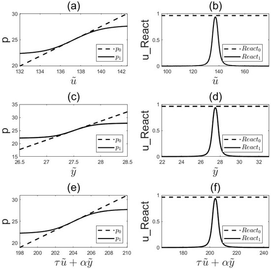
However, according to Item (1) in Appendix A.6, ${u\_React}_1$ is not constant and varies continuously with the private signal $\tilde{u}$ and noise trading volume $\tilde{y}$. Figure 1 illustrates the variability and continuity of ${u\_React}_1$, showing that ${u\_React}_1<{u\_React}_0$.

Figure 1. Take the value of $\gamma =3, {\sigma }_{\epsilon }^2=1, {\sigma }_u^2=6, {\sigma }_y^2=5, {\mu }_0=25, x_I=0.4, Z=25, \overline{v}=28, \underset{\_}{v}=22$. In (a,b), we take $\tilde{y}=10$, showing the impact of increasing $\tilde{u}$ on price and its sensitivity, respectively. In (c,d), we take $\tilde{u}=6$, showing the impact of increasing $\tilde{y}$ on price and its sensitivity, respectively. In (e,f), we show the impact of increasing the linear combination $\tau \tilde{u}+\alpha \tilde{y}$ on price and its sensitivity, respectively.

In summary, the comparison implies that disclosure of range information can cause the reaction of market price to private signal to no longer be constant, varying continuously with private signal and noise trading volume. In the models in the related literature, the reaction of price is usually constant—or piecewise constant—with private signal and noise trading, such as in the works of Kodres and Pritsker (2002) [30], Easley et al. (2014) [7], and Mondria et al. (2022) [23]. As such, our main model reveals a new pattern of market price reactions that has rarely been recorded in the existing literature.

Equation (17) shows that the sensitivity of price $p_1$ depends on $\left[ \underset{\_}{v} ,\overline{v}\right]$ and $\tau \tilde{u}+\alpha \tilde{y}$, where $\tau \tilde{u}+\alpha \tilde{y}$ is a linear combination of the private signal and noise trading volume.

Now we suppose the length of the disclosed range $L$ is fixed. For reflecting the relative position of $\left[ \underset{\_}{v} ,\overline{v}\right]$ and the linear combination $\tau \tilde{u}+\alpha \tilde{y}$, we define the distance $d$ between them as

$$d\triangleq \left\{\begin{array}{c}\underset{\_}{v}-\left(\tau \tilde{u}+\alpha \tilde{y}\right), if \tau \tilde{u}+\alpha \tilde{y}<\underset{\_}{v} \\ 0, if \tau \tilde{u}+\alpha \tilde{y}\in \left[ \underset{\_}{v} ,\overline{v}\right] \\ \left(\tau \tilde{u}+\alpha \tilde{y}\right)-\overline{v}, if \tau \tilde{u}+\alpha \tilde{y}>\overline{v} \end{array}\right.$$

It is apparent that the sensitivity of price to private signal varies with distance $d$. We give the following lemma, the proof of which can be seen in Appendix A.8.

Lemma 2. 

${\mathit{H}}_{\left[ \underset{\_}{v} ,\overline{v}\right]}\left(\tau \tilde{u}+\alpha \tilde{y}+\beta \right)>0$and $\underset{d\to +\infty }{\mathrm{l}\mathrm{i}\mathrm{m}}{\mathit{H}}_{\left[ \underset{\_}{v} ,\overline{v}\right]}\left(\tau \tilde{u}+\alpha \tilde{y}+\beta \right)=0.$

Based on Lemma 2, we have

$$\underset{d\to +\infty }{\mathrm{l}\mathrm{i}\mathrm{m}}{u\_React}_1=\underset{d\to +\infty }{\mathrm{l}\mathrm{i}\mathrm{m}}\tau ·{\mathit{H}}_{\left[ \underset{\_}{v} ,\overline{v}\right]}\left(\tau \tilde{u}+\alpha \tilde{y}+\beta \right)=0,$$

(18)

which implies the sensitivity of price to private signal will approach zero when the distance between $\left[ \underset{\_}{v} ,\overline{v}\right]$ and $\tau \tilde{u}+\alpha \tilde{y}$ is very long. In other words, when the linear combination $\tau \tilde{u}+\alpha \tilde{y}$ deviates heavily from the disclosed range $\left[ \underset{\_}{v} ,\overline{v}\right]$, market price will hardly react to a variation in private signal. The intuition behind this result is that the reliability of private signals in conveying asset value becomes very low for investors when the linear combination $\tau \tilde{u}+\alpha \tilde{y}$ deviates heavily from the possible range of asset value. In this scenario, investors almost no longer rely on the signal to evaluate asset value. As such, a variation in the signal may hardly affect investors’ trading decisions and then the market price.

Now we suppose the length of range information $L$ is variable. According to Item (3) in Appendix A.6, we derive

$$\underset{\begin{array}{c} \underset{\_}{v}\to -\infty \\ \overline{v}\to +\infty \end{array}}{\lim }{u\_React}_1=\underset{\begin{array}{c} \underset{\_}{v}\to -\infty \\ \overline{v}\to +\infty \end{array}}{\mathrm{l}\mathrm{i}\mathrm{m}}\tau ·{\mathit{H}}_{\left[ \underset{\_}{v} ,\overline{v}\right]}\left(\tau \tilde{u}+\alpha \tilde{y}+\beta \right)=\tau ={u\_React}_0.$$

This means the impact of range information disclosure on the price sensitivity will approach zero when the disclosed range is very rough. Since ${u\_React}_0>{u\_React}_1$, the price sensitivity has an overall upward trend when the disclosed range becomes increasingly rougher. Intuitively, as the range information becomes rougher—that is, its precision reduces—investors’ trading decisions will rely more on the private signal and, in turn, price will be more sensitive to it.

4.3. The Sensitivity of Price to Range Information

We analyze the market price reaction when the disclosed range varies, which is regarded as its sensitivity to range information. Firstly, we suppose the private signal $\tilde{u}$, noise trading $\tilde{y}$, and the lower bound $\underset{\_}{v}$ are fixed, and discuss the reaction of market price when the disclosed upper bound $\overline{v}$ varies.

Define the sensitivity of price to the upper bound as

$${\overline{v}\_React}_1\triangleq {\displaystyle \frac{\partial p_1}{\partial \overline{v}}},$$

which can measure the reaction of price when the disclosed upper bound increases by one unit. According to Item (7) in Appendix A.2,

$${\overline{v}\_React}_1={\displaystyle \frac{\partial {\mathit{J}}_{\left[ \underset{\_}{v}, \overline{v} \right]}\left(\tau \tilde{u}+\alpha \tilde{y}+\beta \right)}{\partial \overline{v}}}>0.$$

(19)

As such, the price always increases with the upper bound $\overline{v}$; that is, the price will rise if a higher $\overline{v}$ is released to investors. Our intuition is that a higher upper bound implies the asset value may reach a higher level in future and, in turn, investors’ expectation of its value will also rise. Denote the distance between the linear combination $\tau \tilde{u}+\alpha \tilde{y}$ and $\overline{v}$ by $d_{\overline{v}}$, that is, $d_{\overline{v}}=\left|\overline{v}-(\tau \tilde{u}+\alpha \tilde{y})\right|$. For the scale of the sensitivity ${\overline{v}\_react}_1$, we have the following proposition, the proof of which is given in Appendix A.9.

Proposition 3. 

If$\overline{v}$is high, such that$\overline{v}>\tau \tilde{u}+\alpha \tilde{y}$, then we have

$$\underset{d_{\overline{v}}\to +\infty }{\lim }{\overline{v}\_React}_1=\underset{d_{\overline{v}}\to +\infty }{\mathrm{l}\mathrm{i}\mathrm{m}}{\displaystyle \frac{\partial {\mathit{J}}_{\left[ \underset{\_}{v} ,\overline{v} \right]}\left(\tau \tilde{u}+\alpha \tilde{y}+\beta \right)}{\partial \overline{v}}}=0,$$

which implies a variation in the disclosed upper bound$\overline{v}$can hardly affect the asset price when$\overline{v}$far exceeds the linear combination$\tau \tilde{u}+\alpha \tilde{y}$.

Although we have shown that raising the released upper bound $\overline{v}$ can boost the asset price, Proposition 3 further suggests that increasingly raising $\overline{v}$ is almost unable to increase the price if $\overline{v}$ has far exceeded the linear combination $\tau \tilde{u}+\alpha \tilde{y}$.

Second, we suppose the private signal $\tilde{u}$, noise trading $\tilde{y}$, and the upper bound $\overline{v}$ are fixed, and discuss the reaction of market price when the disclosed lower bound $\underset{\_}{v}$ varies.

Define the sensitivity of price to the lower bound as

$${\underset{\_}{v}\_React}_1\triangleq {\displaystyle \frac{\partial p_1}{\partial \underset{\_}{v}}},$$

which can measure the price reaction when the disclosed lower bound increases by one unit. According to Item (7) in Appendix A.2,

$${\underset{\_}{v}\_React}_1={\displaystyle \frac{\partial {\mathit{J}}_{\left[ \underset{\_}{v} ,\overline{v} \right]}\left(\tau \tilde{u}+\alpha \tilde{y}+\beta \right)}{\partial \underset{\_}{v}}}>0.$$

(20)

As such, the price will rise if a higher $\underset{\_}{v}$ is released to investors. Our intuition is that a higher lower bound implies the maximum loss investors may suffer in future declines; in turn, investors’ expectation of its value will also rise. Denote the distance between the linear combination $\tau \tilde{u}+\alpha \tilde{y}$ and $\underset{\_}{v}$ by $d_{\underset{\_}{v}}$, that is, $d_{\underset{\_}{v}}=\left|\tau \tilde{u}+\alpha \tilde{y}-\underset{\_}{v}\right|$. Then, we have the following proposition, the proof of which is given in Appendix A.10.

Proposition 4. 

If$\underset{\_}{v}$is low, such that $\underset{\_}{v}<\tau \tilde{u}+\alpha \tilde{y}$, then we have

$$\underset{d_{\underset{\_}{v}}\to +\infty }{\lim }{\underset{\_}{v}\_React}_1=\underset{d_{\underset{\_}{v}}\to +\infty }{\mathrm{l}\mathrm{i}\mathrm{m}}{\displaystyle \frac{\partial {\mathit{J}}_{\left[ \underset{\_}{v} ,\overline{v} \right]}\left(\tau \tilde{u}+\alpha \tilde{y}+\beta \right)}{\partial \underset{\_}{v}}}=0,$$

which implies that a variation in the disclosed lower bound$\underset{\_}{v}$can hardly affect the asset price when$\underset{\_}{v}$is far below the linear combination$\tau \tilde{u}+\alpha \tilde{y}$.

Although we have shown that reducing the released lower bound $\underset{\_}{v}$ can decrease the asset price, Proposition 4 further suggests that increasingly reducing $\overline{v}$ is almost unable to decrease the price if $\overline{v}$ has been far below the linear combination $\tau \tilde{u}+\alpha \tilde{y}$.

Third, we suppose the private signal $\tilde{u}$, noise trading $\tilde{y}$, and the length of range information $L$ are fixed, and discuss the reaction of market price when the disclosed range moves. As a reminder, the midpoint of $\left[ \underset{\_}{v} ,\overline{v} \right]$ is denoted by $v_m$.

Since the length of $\left[ \underset{\_}{v} ,\overline{v} \right]$ is fixed, we can use the variation in its midpoints to measure a movement of the range. A one-unit increase (decrease) in the midpoint means a one-unit upward (downward) movement in the disclosed range and vice versa. Thus, we can measure the sensitivity of price to movement in the disclosed range by

$${Range\_React}_1\triangleq {\displaystyle \frac{\partial p_1}{\partial v_m}}.$$

We give the following lemma to specify the sensitivity ${Range\_react}_1$. Its proof is given in Appendix A.11.

Lemma 3. 

For any given$\tilde{u}$, $\tilde{y}$and $L$, we have

$${Range\_React}_1={\displaystyle \frac{\partial {\mathit{J}}_{\left[ \underset{\_}{v} ,\overline{v} \right]}\left(\tau \tilde{u}+\alpha \tilde{y}+\beta \right)}{\partial v_m}}=1-{\mathit{H}}_{\left[ \underset{\_}{v} ,\overline{v} \right]}\left(\tau \tilde{u}+\alpha \tilde{y}+\beta \right).$$

According to Items (2) and (3) in Appendix A.6, we have $0<{\mathit{H}}_{\left[ \underset{\_}{v} ,\overline{v} \right]}\left(\tau \tilde{u}+\alpha \tilde{y}+\beta \right)<1$ and then

$$1>{Range\_React}_1>0,$$

which means if the disclosed range move upwards, the asset price will rise and the increase in its price will be less than the movement of the disclosed range. In other words, disclosing a higher range will lead to a higher market price.

According to Lemmas 2 and 3, it follows that

$$\underset{d\to +\infty }{\mathrm{l}\mathrm{i}\mathrm{m}}{Range\_React}_1=1-\underset{d\to +\infty }{\mathrm{l}\mathrm{i}\mathrm{m}}{\mathit{H}}_{\left[ \underset{\_}{v} ,\overline{v}\right]}\left(\tau \tilde{u}+\alpha \tilde{y}+\beta \right)=1,$$

(21)

which means an upward movement in the disclosed range will cause the asset price to rise by nearly the same amount when $\tau \tilde{u}+\alpha \tilde{y}$ deviates heavily from the disclosed range. The intuition behind this result is that the reliability of private signal in reflecting asset value becomes very low for investors when $\tau \tilde{u}+\alpha \tilde{y}$ deviates heavily from the range. In this case, investors almost wholly rely on the disclosed range to assess the asset value. Thus, a movement of the disclosed range can efficiently impact investors’ assessment of asset value and, in turn, price.

Combining Equations (18) and (21), we put forward the following proposition.

Proposition 5. 

If the linear combination$\tau \tilde{u}+\alpha \tilde{y}$is distant from the disclosed range, a variation in private signal regarding asset value may hardly affect its price, whereas a movement in the disclosed range can impact price efficiently.

Furthermore, we can compare the reaction of asset price to variation in the private signal with that to movement in the disclosed range. For any given private signal $\tilde{u}$, noise trading volume $\tilde{y}$, and disclosed range $\left[ \underset{\_}{v} ,\overline{v} \right]$, if ${\mathit{H}}_{\left[ \underset{\_}{v} ,\overline{v}\right]}\left(\tau \tilde{u}+\alpha \tilde{y}+\beta \right)<{\displaystyle \frac{1}{1+\tau }}$, then ${u\_React}_1<{Range\_React}_1$, which means the asset price has a larger reaction to movement in the disclosed range. If ${\mathit{H}}_{\left[ \underset{\_}{v} ,\overline{v}\right]}\left(\tau \tilde{u}+\alpha \tilde{y}+\beta \right)>{\displaystyle \frac{1}{1+\tau }}$, then ${u\_React}_1>{Range\_React}_1$, which means the price has a larger reaction to variation in the private signal. If $\underset{t\in R}{\sup }{\mathit{H}}_{\left[ \underset{\_}{v} ,\overline{v}\right]}\left(t\right)<{\displaystyle \frac{1}{1+\tau }}$, then ${u\_React}_1<{Range\_React}_1$ holds for any $\tilde{u}$ and $\tilde{y}$, which implies the reaction of asset price to movement in the disclosed range is always larger than that to variation in the private signal. However, given Proposition 5, the reaction of asset price to variation in the private signal cannot always be larger than that to movement in the disclosed range.

4.4. Market Liquidity

According to the related literature, such as the work of Goldstein and Yang (2017) [25], market liquidity is defined as

$$Liquidity\triangleq {\left({\displaystyle \frac{\partial p}{\partial \tilde{y}}}\right)}^{-1}.$$

A greater market liquidity means noise trading $y$ has a smaller impact on the market price and the market is regarded to be deeper and more liquid.

In the equilibrium of the baseline model, the market liquidity is

$${Liquidity}_0={\left({\displaystyle \frac{\partial p_0}{\partial \tilde{y}}}\right)}^{-1}={\displaystyle \frac{1}{\alpha }}={\displaystyle \frac{x_I}{\gamma {\sigma }_{\epsilon }^2}}{\left(1-{\displaystyle \frac{x_U}{1+\frac{x_I^2{\sigma }_u^2}{{\gamma }^2{\sigma }_{\epsilon }^4{\sigma }_y^2}+\frac{x_I{\sigma }_u^2}{{\sigma }_{\epsilon }^2}}}\right)}^{-1}.$$

(22)

In the equilibrium of our main model, according to Item (2) in Appendix A.2, the market liquidity is

$${Liquidity}_1={\left({\displaystyle \frac{\partial p_1}{\partial \tilde{y}}}\right)}^{-1}={\displaystyle \frac{1}{\alpha }}\cdot {\displaystyle \frac{1}{ {\mathit{H}}_{\left[ \underset{\_}{v} ,\overline{v}\right]}\left(\tau \tilde{u}+\alpha \tilde{y}+\beta \right) }}.$$

(23)

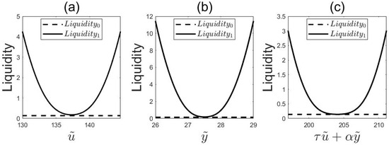
${Liquidity}_0$ is constant; that is, it is independent of the private signal $\tilde{u}$ and noise trading $\tilde{y}$. According to Item (1) in Appendix A.6, ${Liquidity}_1$ is not constant and varies continuously with $\tilde{u}$ and $\tilde{y}$. Figure 2 illustrates the variability and continuity of ${Liquidity}_1$.

Figure 2. Take the value of $\gamma =3,{\sigma }_{\epsilon }^2=1,{\sigma }_u^2=6,{\sigma }_y^2=5,{\mu }_0=25,x_I=0.4,Z=25,\overline{v}=27,\underset{\_}{v}=23$. In (a), we take $\tilde{y}=10$ and show the impact of increasing $\tilde{u}$ on liquidity. In (b), we take $\tilde{u}=6$ and show the impact of increasing $\tilde{y}$ on liquidity. In (c), we show the impact of increasing the linear combination $\tau \tilde{u}+\alpha \tilde{y}$ on liquidity.

According to Item (3) in Appendix A.6, we have

$${Liquidity}_1={\displaystyle \frac{1}{\alpha }}\cdot {\displaystyle \frac{1}{ {\mathit{H}}_{\left[ \underset{\_}{v} ,\overline{v}\right]}\left(\tau \tilde{u}+\alpha \tilde{y}+\beta \right) }}>{\displaystyle \frac{1}{\alpha }}={Liquidity}_0$$

holds for any $\tilde{u}$, $\tilde{y}$, $\underset{\_}{v}$, $\overline{v}$ with $\underset{\_}{v}<\overline{v}$. Thus, it is shown that disclosing range information would increase market liquidity, which is illustrated by Figure 2.

In the models presented in the related literature, market liquidity is usually constant—or piecewise constant—with private signal and noise trading. The comparison between ${Liquidity}_0$ and ${Liquidity}_1$ shows that disclosing range information would cause market liquidity to vary continuously with private signal and noise trading volume. This pattern of liquidity has also rarely been recorded in the existing related literature.

However, according to Item (3) in Appendix A.6,

$$\underset{\begin{array}{c}\overline{v}\to +\infty \\ \underset{\_}{v}\to -\infty \end{array}}{\lim }{Liquidity}_1={\displaystyle \frac{1}{\alpha }}={Liquidity}_0,$$

which means the effect of range information disclosure on market liquidity will approach zero if the disclosed range is very rough. Since ${Liquidity}_1>{Liquidity}_0$, market liquidity has an overall downward trend when the disclosed range information becomes increasingly rougher.

The completeness of investors’ information is an important factor determining market liquidity. Generally speaking, market liquidity increases with information completeness. Disclosing range information can improve the completeness of investors’ information and then raise market liquidity. If the disclosed range is very rough, then it will provide investors with little incremental information and can hardly improve their information completeness. As a result, disclosing a very rough range will generate a minor impact on market liquidity.

Using Equation (23) and Lemma 2, we can derive

$$\underset{d\to +\infty }{\lim }{Liquidity}_1=\underset{d\to +\infty }{\mathrm{l}\mathrm{i}\mathrm{m}}{\displaystyle \frac{1}{\alpha }}\cdot {\displaystyle \frac{1}{ {\mathit{H}}_{\left[ \underset{\_}{v} ,\overline{v}\right]}\left(\tau \tilde{u}+\alpha \tilde{y}+\beta \right) }}=+\infty ,$$

which implies the market will be extremely liquid when the linear combination of private signal and noise trading volume $\tau \tilde{u}+\alpha \tilde{y}$ is far away from the disclosed range.

4.5. Asset Premium

Asset premium is usually regarded as a cost of capital. According to Huang et al. (2020) [24], it is defined as the expected difference between the payoff of an asset and its market price. We denote asset premium by ${Premium}_0$ for the case where range information is not disclosed and by ${Premium}_1(\underset{\_}{v} ,\overline{v})$ for the case where the asset value range is disclosed as $\left[ \underset{\_}{v} ,\overline{v}\right]$. According to Equations (11) and (15), we have

$${Premium}_0=E\left[v-p_0\right]=\left(1-\tau \right){\mu }_0-\beta$$

and

$${Premium}_1\left(\underset{\_}{v}, \overline{v}\right)=E\left[v-p_1\right]={\mu }_0-E\left[{\mathit{J}}_{\left[\underset{\_}{v} ,\overline{v} \right]}\left(\tau u+\alpha y+\beta \right)\right].$$

In Section 4.2, for any given $\tilde{u}$ and $\tilde{y}$, the price $p_1$ will increase when $\underset{\_}{v}$ or $\overline{v}$ is raised. Thus, an increase in the lower and upper bounds of the disclosed range can both reduce the asset premium ${Premium}_1\left(\underset{\_}{v} ,\overline{v}\right)$. Similarly, it is also proved in Section 4.3 that an upward movement in the range $\left[ \underset{\_}{v} ,\overline{v}\right]$ can raise the price $p_1$ for any given $\tilde{u}$ and $\tilde{y}$. Thus, disclosing a higher range will also reduce the asset premium ${Premium}_1\left(\underset{\_}{v} ,\overline{v}\right)$.

For any given range $\left[ \underset{\_}{v} ,\overline{v}\right]$, we put forward the following proposition, with which we can judge whether disclosing the range will raise or decrease the asset premium.

Proposition 6. 

Suppose

$$B_0\triangleq \beta +{\mu }_0·\tau ={\mu }_0-Z\gamma {\sigma }_{\epsilon }^2-{\displaystyle \frac{Z{\gamma }^3{x}_U{\sigma }_u^2{\sigma }_{\epsilon }^4{\sigma }_y^2}{{\gamma }^2{\sigma }_{\epsilon }^4{\sigma }_y^2+x_I^2{\sigma }_u^2+{\gamma }^3{x}_I{\sigma }_u^2{\sigma }_{\epsilon }^2{\sigma }_y^2}}.$$

(24)

If the midpoint of the disclosed range$v_m=B_0$, then${Premium}_1\left(\underset{\_}{v}, \overline{v}\right)={Premium}_0$. If$v_m<B_0$, then${Premium}_1\left(\underset{\_}{v}, \overline{v}\right)>{Premium}_0$. If$v_m>B_0$, then${Premium}_1\left(\underset{\_}{v}, \overline{v}\right)<{Premium}_0$.

The proof can be seen in Appendix A.12. Proposition 6 suggests that whether disclosing range information can reduce capital costs depends on the midpoint of the disclosed range. Disclosing a range with a midpoint higher (lower) than $B_0$ will reduce (raise) capital cost. As such, $B_0$ can be regarded as a benchmark for assessing the effect of range information disclosure on capital cost. If we aim to prevent the disclosure of range information from raising capital cost, the midpoint of the disclosed range should be $B_0$ or higher than $B_0$.

According to Equation (24), we have

$${\displaystyle \frac{\partial B_0}{\partial {\sigma }_{\epsilon }^2}}<0, {\displaystyle \frac{\partial B_0}{\partial {\sigma }_y^2}}<0, {\displaystyle \frac{\partial B_0}{\partial {\sigma }_u^2}}<0,{\displaystyle \frac{\partial B_0}{\partial Z}}<0, {\displaystyle \frac{\partial B_0}{\partial x_I}}>0, {\displaystyle \frac{\partial B_0}{\partial {\mu }_0}}>0,$$

(25)

that is, the benchmark $B_0$ decreases with ${\sigma }_{\epsilon }^2$, ${\sigma }_y^2$, ${\sigma }_u^2$, $Z$ and increases with $x_I$, ${\mu }_0$, which gives rise to the following corollary.

Corollary 2. 

If we aim to prevent the disclosure of range information from raising capital cost, we need to disclose a higher range when

(1) 

The precision of the private signal is higher, that is, ${\sigma }_{\epsilon }^2$is smaller;

(2) 

The size of noise trading in the market ${\sigma }_y^2$is smaller;

(3) 

The informativeness of the private signal ${\sigma }_u^2$is smaller;

(4) 

The supply of risky asset $Z$is smaller;

(5) 

The proportion of informed traders $x_I$is larger;

(6) 

The unconditional mean of risky asset value ${\mu }_0$is higher.

In other words, for a certain asset value range $\left[\underset{\_}{v},\overline{v}\right]$, its disclosure to market is more likely to cause an increase in asset premium under the six conditions listed in Corollary 2.

Preventing the asset premium from rising implies preventing the expected asset price from decreasing. In reality, the expectation of asset price is $B_0$ when range information is not disclosed, that is,

$$E\left[p_0\right]=\beta +{\mu }_0·\tau =B_0.$$

As such, the expectation of asset price $E\left[p_0\right]$ will be higher under the six conditions listed in Corollary 2. The intuition behind this is that disclosing a higher range is necessary to maintain a high level of $E\left[p_0\right]$ under these conditions, that is, to prevent it from decreasing.

We analyze the reaction of the asset premium when the disclosed range varies, which is regarded as its sensitivity to range information.

The sensitivity of the asset premium to the upper and lower bounds is, respectively,

$${\displaystyle \frac{\partial {Premium}_1\left(\underset{\_}{v} ,\overline{v}\right)}{\partial \overline{v}}}=-{\displaystyle \frac{\partial }{\partial \overline{v}}}E\left[{\mathit{J}}_{\left[\underset{\_}{v} ,\overline{v} \right]}\left(\tau u+\alpha y+\beta \right)\right]$$

and

$${\displaystyle \frac{\partial {Premium}_1\left(\underset{\_}{v} ,\overline{v}\right)}{\partial \underset{\_}{v}}}=-{\displaystyle \frac{\partial }{\partial \underset{\_}{v}}}E\left[{\mathit{J}}_{\left[\underset{\_}{v} ,\overline{v} \right]}\left(\tau u+\alpha y+\beta \right)\right].$$

They measure the reaction of the asset premium when $\overline{v}$ and $\underset{\_}{v}$ vary, respectively.

The distance between ${\mu }_0$ and $\overline{v}$ and the distance between ${\mu }_0$ and $\underset{\_}{v}$ are denoted by $D_{\overline{v}}$ and $D_{\underset{\_}{v}}$, respectively. As for the two sensitivities above, we have the following proposition, the proof of which is given in Appendix A.13.

Proposition 7. 

If$\overline{v}$is high, such that$\overline{v}>{\mu }_0$, then we have

$$\underset{D_{\overline{v}}\to +\infty }{\lim }{\displaystyle \frac{\partial {Premium}_1\left(\underset{\_}{v} ,\overline{v}\right)}{\partial \overline{v}}}=0.$$

Additionally, if $\underset{\_}{v}$is low, such that $\underset{\_}{v}<{\mu }_0$, then we have

$$\underset{D_{\underset{\_}{v}}\to +\infty }{\lim }{\displaystyle \frac{\partial {Premium}_1\left(\underset{\_}{v} ,\overline{v}\right)}{\partial \underset{\_}{v}}}=0.$$

According to Proposition 7, we reveal that a movement in the disclosed upper bound $\overline{v}$ can hardly affect asset premium when $\overline{v}$ far exceeds the unconditional mean of asset value ${\mu }_0$, while a movement in the disclosed lower bound $\underset{\_}{v}$ can hardly affect asset premium when $\underset{\_}{v}$ is far below ${\mu }_0$.

Suppose the length of range information $L$ is fixed, and we focus on the reaction of asset premium when the disclosed range moves and ${\mu }_0$ varies. To reflect the relative position of $\left[ \underset{\_}{v} ,\overline{v}\right]$ and the unconditional mean of asset value ${\mu }_0$, we define the distance $D$ between them as

$$D\triangleq \left\{\begin{array}{c}\underset{\_}{v}-{\mu }_0, \hspace{1em}if {\mu }_0<\underset{\_}{v} \\ 0, if {\mu }_0\in \left[ \underset{\_}{v} ,\overline{v}\right] \\ {\mu }_0-\overline{v}, if {\mu }_0>\overline{v} \end{array}\right.$$

As a reminder, the midpoint of $\left[ \underset{\_}{v} ,\overline{v} \right]$ is denoted by $v_m$. Since the length of the range is fixed, its movement can be measured by the variation in its midpoint. Then, the sensitivity of the asset premium to movement in the disclosed range can be measured by

$${\displaystyle \frac{\partial {Premium}_1\left(\underset{\_}{v} ,\overline{v}\right)}{\partial v_m}}=-{\displaystyle \frac{\partial }{\partial v_m}}E\left[{\mathit{J}}_{\left[\underset{\_}{v}, \overline{v} \right]}\left(\tau u+\alpha y+\beta \right)\right].$$

Meanwhile, its sensitivity to variation in ${\mu }_0$ can be measured by

$${\displaystyle \frac{\partial {Premium}_1\left(\underset{\_}{v}, \overline{v}\right)}{\partial {\mu }_0}}=-{\displaystyle \frac{\partial }{\partial {\mu }_0}}E\left[{\mathit{J}}_{\left[\underset{\_}{v}, \overline{v} \right]}\left(\tau u+\alpha y+\beta \right)\right].$$

We have the following proposition, the proof of which is given in Appendix A.14.

Proposition 8. 

If the parameters$Z, \gamma , L, {\sigma }_u^2, {\sigma }_{\epsilon }^2, {\sigma }_y^2,$$x_I$are all fixed, then

$$\underset{D\to +\infty }{\mathrm{l}\mathrm{i}\mathrm{m}}{\displaystyle \frac{\partial {Premium}_1\left(\underset{\_}{v} ,\overline{v}\right)}{\partial {\mu }_0}}=0, \underset{D\to +\infty }{\mathrm{l}\mathrm{i}\mathrm{m}}{\displaystyle \frac{\partial {Premium}_1\left(\underset{\_}{v} ,\overline{v}\right)}{\partial v_m}}=-1.$$

Proposition 8 reveals that if the unconditional mean of asset value ${\mu }_0$ is distant from the disclosed range, a variation in ${\mu }_0$ can hardly affect the asset premium, whereas a movement in the disclosed range can impact the asset premium efficiently. More specifically, an upward movement in the range will cause the asset premium to decrease by nearly the same amount when ${\mu }_0$ is far away from the range.

Regarding asset premium, we have the following proposition about the disclosure of rough range information, proof of which is given in Appendix A.15.

Proposition 9. 

If the disclosed range is very rough, the effect of its disclosure on asset premium will almost vanish and the sensitivity of asset premium to movement in the disclosed range will almost vanish, that is,

$$\begin{gathered} \underset{\begin{array}{c}\overline{v}\to +\infty \\ \underset{\_}{v}\to -\infty \end{array}}{\mathrm{l}\mathrm{i}\mathrm{m}}{Premium}_1\left(\underset{\_}{v} ,\overline{v}\right)={Premium}_0, \\ \underset{\begin{array}{c}\overline{v}\to +\infty \\ \underset{\_}{v}\to -\infty \end{array}}{\mathrm{l}\mathrm{i}\mathrm{m}}{\displaystyle \frac{\partial {Premium}_1\left(\underset{\_}{v} ,\overline{v}\right)}{\partial v_m}}=0. \end{gathered}$$

In summary, if the range is very rough, its disclosure will have a negligible impact on market price and asset premium.

5. Conclusions

This study reveals that the disclosure of range information can increase or decrease market price, which depends on the midpoint of the disclosed range. If the midpoint is higher (lower) than a specified benchmark, the disclosure will raise (reduce) the price. The benchmark increases with noise trading demand and with the private signal received by informed traders.

We also find that disclosing range information will decrease the sensitivity of market price to private signal and increase market liquidity. Its disclosure can also change the pattern of market price reacting to private signal and noise trading, and the pattern of market liquidity varying with them. The reaction of price to private signal will almost vanish and market liquidity will approach infinity when the linear combination of private signal and noise trading volume deviates heavily from the disclosed range. The sensitivity of price to private signal displays an overall upward trend, and market liquidity follows an overall downward trend, when the range information becomes increasingly rough.

Additionally, the disclosure of range information can increase or decrease the asset premium, which depends on the midpoint of the disclosed range. If the midpoint is higher (lower) than a specified benchmark, the disclosure will reduce (raise) the asset premium. The benchmark decreases with noise trading size, private signal informativeness, and risky asset supply, and increases with the precision of private signal, the proportion of informed traders, and the unconditional mean of risky asset value.

This study further shows that an increase in the upper or lower bound of the disclosed range and an upward movement in the range can both raise asset price and then reduce asset premium. However, the impact of a variation in the upper bound on asset price will approach zero when it far exceeds the linear combination of private signal and noise trading volume; in addition, the impact of a variation in the lower bound on asset price will also approach zero when it is far below the linear combination of private signal and noise trading volume.

In the scenario where the linear combination of private signal and noise trading volume is distant from the disclosed range, a variation in private signal can hardly affect asset price, whereas a movement in the disclosed range can impact the price efficiently. Similarly, when the unconditional mean of the asset value is distant from the disclosed range, a variation in the unconditional mean can hardly affect the asset premium, whereas a movement in the disclosed range can impact the asset premium efficiently.

It is also revealed that range information disclosure will have a negligible impact on market price, liquidity and asset premium if the disclosed range is very rough.

In summary, range information disclosure can significantly affect the asset market; however, the effect depends on the precision and position of the disclosed range—especially its distance from the linear combination of private signal and noise trading volume—and its distance from the unconditional asset value mean.

Based on these conclusions, we have some suggestions about information disclosure for risk management and improvement of market quality. First, disclosing range information may reduce the sensitivity of market price and improve market liquidity in a specific parameter range. Second, in order to mitigate the risk of market price decline, we should reduce disclosing range information when the private signal regarding asset value is optimistic or the noise trading demand is larger. Third, to mitigate the risk of an increase in capital cost, we should reduce disclosing range information when (1) the precision of the private signal is high, (2) the proportion of informed traders is large, (3) the size of noise trading is small, (4) the informativeness of the private signal is small, and (5) the supply of the risky asset is small.

Appendix A.1. The Calculation of Equation (2)

Define a conditional distribution $w\triangleq v\left|(u=\tilde{u}) \right.$, then $w~N(\tilde{u},{\sigma }_{\epsilon }^2)$. The cumulative distribution and probability density function of $w$ are denoted by $F_w$ and $f_w$, respectively. The denominator of $U_I\left({\mathrm{\theta }}_I\right)$ is

$$\begin{array}{cc}& E\left[{{\displaystyle 1}}_{\left\{v\in \left[\underset{\_}{v} , \overline{v}\right]\right\}}\left|u=\tilde{u}\right.\right]\\ =& E\left[{{\displaystyle 1}}_{\left\{w\in \left[\underset{\_}{v} , \overline{v}\right]\right\}}\right]\\ =& {\int }_{\underset{\_}{v}}^{\overline{v}}{\displaystyle \frac{1}{\sqrt{2\pi }{\sigma }_{\epsilon }}}{e}^{-{\displaystyle \frac{{(x-\tilde{u})}^2}{2{\sigma }_{\epsilon }^2}}}dx \\ =& \mathsf{\Psi }\left({\displaystyle \frac{\overline{v}-\tilde{u}}{{\sigma }_{\epsilon }}}\right)-\mathsf{\Psi }\left({\displaystyle \frac{\underset{\_}{v}-\tilde{u}}{{\sigma }_{\epsilon }}}\right).\end{array}$$

The numerator of $U_I\left({\mathrm{\theta }}_I\right)$ is

$$\begin{array}{ll}& E\left[-e^{-\gamma \left(D_0+{\mathrm{\theta }}_I\left(v-p\right)\right)}{{\displaystyle 1}}_{\left\{v\in \left[\underset{\_}{v} , \overline{v}\right]\right\}}\left|u=\tilde{u}\right.\right]\\ =& E\left[-e^{-\gamma \left(D_0+{\mathrm{\theta }}_I\left(w-p\right)\right)}{{\displaystyle 1}}_{\left\{w\in \left[\underset{\_}{v} , \overline{v}\right]\right\}}\right]\\ =& -e^{-\gamma D_0+\gamma p{\mathrm{\theta }}_I}{\int }_{\underset{\_}{v}}^{\overline{v}}{e}^{-\gamma {\mathrm{\theta }}_{I}x}·{\displaystyle \frac{1}{\sqrt{2\pi }{\sigma }_{\epsilon }}}{e}^{-{\displaystyle \frac{{(x-\tilde{u})}^2}{2{\sigma }_{\epsilon }^2}}}dx\\ =& -e^{-\gamma D_0+\gamma \left(p-\tilde{u}\right){\mathrm{\theta }}_I+{\displaystyle \frac{{\gamma }^2{\sigma }_{\epsilon }^2{\theta }_I^2}{2}}}\left[F_w\left(\overline{v}+\gamma {\sigma }_{\epsilon }^2{\mathrm{\theta }}_I\right)-F_w\left(\underset{\_}{v}+\gamma {\sigma }_{\epsilon }^2{\mathrm{\theta }}_I\right)\right]\\ =& -e^{-\gamma D_0+\gamma \left(p-\tilde{u}\right){\mathrm{\theta }}_I+{\displaystyle \frac{{\gamma }^2{\sigma }_{\epsilon }^2{\theta }_I^2}{2}}}\left[\mathsf{\Psi }\left({\displaystyle \frac{\overline{v}+\gamma {\sigma }_{\epsilon }^2{\mathrm{\theta }}_I-\tilde{u}}{{\sigma }_{\epsilon }}}\right)-\mathsf{\Psi }\left({\displaystyle \frac{\underset{\_}{v}+\gamma {\sigma }_{\epsilon }^2{\mathrm{\theta }}_I-\tilde{u}}{{\sigma }_{\epsilon }}}\right)\right].\end{array}$$

Appendix A.2. Some Properties of the Function ${\mathit{J}}_{\left[\mathit{a},\mathit{b}\right]}\left(\mathit{t}\right)$

As a reminder, $\epsilon ~N(0,{\sigma }_{\epsilon }^2)$. Its cumulative distribution and probability density function are denoted by $F_{\epsilon }$ and $f_{\epsilon }$, respectively. For any fixed $a, b\in R$ with $b>a$, the following properties hold.

(1)

$a<{\mathit{J}}_{\left[a,\mathrm{b}\right]}\left(t\right)<b$.

(2)

${\mathit{J}}_{\left[a,\mathrm{b}\right]}\prime \left(t\right)={\mathit{H}}_{\left[a,\mathrm{b}\right]}\left(t\right)$, where

$${\mathit{H}}_{\left[a,\mathrm{b}\right]}\left(t\right)\triangleq {\displaystyle \frac{1}{{\sigma }_{\epsilon }^2}}\left[{\displaystyle \frac{{\int }_{ a-t}^{b-t}{x}^2{f}_{\epsilon }\left(x\right)dx}{{\int }_{ a-t}^{b-t}{f}_{\epsilon }\left(x\right)dx}}-{\left({\displaystyle \frac{{\int }_{ a-t}^{b-t}x{f}_{\epsilon }\left(x\right)dx}{{\int }_{ a-t}^{b-t}{f}_{\epsilon }\left(x\right)dx}}\right)}^2\right].$$

(A1)

(3)

$1>{\mathit{J}}_{\left[a,\mathrm{b}\right]}\prime \left(t\right)>0$.

(4)

$\underset{t\to +\mathrm{\infty }}{\lim }{\mathit{J}}_{\left[a,\mathrm{b}\right]}\left(t\right)=b$ and $\underset{t\to -\mathrm{\infty }}{\lim }{\mathit{J}}_{\left[a,\mathrm{b}\right]}\left(t\right)=a$.

(5)

${\mathit{J}}_{\left[a,\mathrm{b}\right]}\left(t\right)$ is continuous with respect to $t,a,b$.

(6)

For any $c\in R$, ${\mathit{J}}_{\left[a,\mathrm{b}\right]}\left(t\right)={\mathit{J}}_{\left[a-c,\mathrm{b}-\mathrm{c}\right]}\left(t-c\right)+c$.

(7)

${\displaystyle \frac{\partial {\mathit{J}}_{\left[a,\mathrm{b}\right]}\left(t\right)}{\partial b}}={\displaystyle \frac{f_{\epsilon }\left(b-t\right){\int }_{a-t}^{b-t}(b-t-x)f_{\epsilon }\left(x\right)dx}{{\left({\int }_{a-t}^{b-t}{f}_{\epsilon }\left(x\right)dx\right)}^2}}>0$, and

${\displaystyle \frac{\partial {\mathit{J}}_{\left[a,\mathrm{b}\right]}\left(t\right)}{\partial a}}={\displaystyle \frac{f_{\epsilon }\left(a-t\right){\int }_{a-t}^{b-t}\left[x-\left(a-t\right)\right]f_{\epsilon }\left(x\right)dx}{{\left({\int }_{a-t}^{b-t}{f}_{\epsilon }\left(x\right)dx\right)}^2}}>0$.

(8)

$\underset{\begin{array}{c}a\to -\infty \\ b\to +\infty \end{array}}{\lim }{\mathit{J}}_{\left[a,\mathrm{b}\right]}\left(t\right)=t$.

Proof. 

We give the proof of Items (1), (3), and (7).

It can be verified that

$${\mathit{J}}_{\left[a,\mathrm{b}\right]}\left(t\right)={\displaystyle \frac{{\int }_{ a-t}^{b-t}x{f}_{\epsilon }\left(x\right)dx}{{\int }_{ a-t}^{b-t}{f}_{\epsilon }\left(x\right)dx}}+t.$$

Then,

$$a=a-t+t<{\mathit{J}}_{\left[a,\mathrm{b}\right]}\left(t\right)<b-t+t=b.$$

As such, Item (1) holds. By some calculations about the derivative of ${\mathit{J}}_{\left[a,\mathrm{b}\right]}\left(·\right)$, we can derive Equation (A1).

$$\begin{array}{cc}{\mathit{J}}_{\left[a,\mathrm{b}\right]}\prime \left(t\right)& ={\displaystyle \frac{\partial }{\partial t}}\left[{\displaystyle \frac{{\int }_{ a-t}^{b-t}x{f}_{\epsilon }\left(x\right)dx}{{\int }_{ a-t}^{b-t}{f}_{\epsilon }\left(x\right)dx}}+t\right]\\ & ={\displaystyle \frac{1}{{\sigma }_{\epsilon }^2}}\left[{\displaystyle \frac{{\int }_{ a-t}^{b-t}{x}^2{f}_{\epsilon }\left(x\right)dx}{{\int }_{ a-t}^{b-t}{f}_{\epsilon }\left(x\right)dx}}-{\left({\displaystyle \frac{{\int }_{ a-t}^{b-t}x{f}_{\epsilon }\left(x\right)dx}{{\int }_{ a-t}^{b-t}{f}_{\epsilon }\left(x\right)dx}}\right)}^2\right].\end{array}$$

Based on Item (2), we have

$$\begin{array}{cc}{\mathit{J}}_{\left[a,\mathrm{b}\right]}\prime \left(t\right)& ={\displaystyle \frac{1}{{\sigma }_{\epsilon }^2}}\left[{\displaystyle \frac{{\int }_{ a-t}^{b-t}{x}^2{f}_{\epsilon }\left(x\right)dx}{{\int }_{ a-t}^{b-t}{f}_{\epsilon }\left(x\right)dx}}-{\left({\displaystyle \frac{{\int }_{ a-t}^{b-t}x{f}_{\epsilon }\left(x\right)dx}{{\int }_{ a-t}^{b-t}{f}_{\epsilon }\left(x\right)dx}}\right)}^2\right]\\ & ={\displaystyle \frac{{\int }_{ a-t}^{b-t}{f}_{\epsilon }\left(x\right)dx-\left(b-t\right)f_{\epsilon }\left(b-t\right)+\left(a-t\right)f_{\epsilon }\left(a-t\right)}{{\int }_{ a-t}^{b-t}{f}_{\epsilon }\left(x\right)dx}}-{\displaystyle \frac{\left(f_{\epsilon }\left(a-t\right)-f_{\epsilon }\left(b-t\right)\right){\int }_{ a-t}^{b-t}x{f}_{\epsilon }\left(x\right)dx}{{\left({\int }_{ a-t}^{b-t}{f}_{\epsilon }\left(x\right)dx\right)}^2}}\\ & =1+{\displaystyle \frac{f_{\epsilon }\left(a-t\right){\int }_{ a-t}^{b-t}\left[\left(a-t\right)-x\right]f_{\epsilon }\left(x\right)dx}{{\left({\int }_{ a-t}^{b-t}{f}_{\epsilon }\left(x\right)dx\right)}^2}}+{\displaystyle \frac{f_{\epsilon }\left(b-t\right){\int }_{ a-t}^{b-t}\left[x-(b-t)\right]f_{\epsilon }\left(x\right)dx}{{\left({\int }_{ a-t}^{b-t}{f}_{\epsilon }\left(x\right)dx\right)}^2}}\\ & <1,\end{array}$$

and

$$\begin{array}{cc}{\mathit{J}}_{\left[a,\mathrm{b}\right]}\prime \left(t\right)& ={\displaystyle \frac{1}{{\sigma }_{\epsilon }^2}}\left[{\displaystyle \frac{{\int }_{a-t}^{b-t}{x}^2{f}_{\epsilon }\left(x\right)dx}{{\int }_{a-t}^{b-t}{f}_{\epsilon }\left(x\right)dx}}-{\left({\displaystyle \frac{{\int }_{a-t}^{b-t}x{f}_{\epsilon }\left(x\right)dx}{{\int }_{a-t}^{b-t}{f}_{\epsilon }\left(x\right)dx}}\right)}^2\right]\\ & ={\displaystyle \frac{{\int }_{a-t}^{b-t}{\left(x-\frac{{\int }_{a-t}^{b-t}x{f}_{\epsilon }\left(x\right)dx}{{\int }_{a-t}^{b-t}{f}_{\epsilon }\left(x\right)dx}\right)}^2{f}_{\epsilon }\left(x\right)dx}{{\sigma }_{\epsilon }^2·{\int }_{a-t}^{b-t}{f}_{\epsilon }\left(x\right)dx}}\\ & >0.\hfill \end{array}$$

So, Item (3) holds.

$$\begin{array}{cc}{\displaystyle \frac{\partial {\mathit{J}}_{\left[a,\mathrm{b}\right]}\left(t\right)}{\partial b}}& ={\displaystyle \frac{\partial }{\partial b}}\left[{\displaystyle \frac{{\int }_{ a-t}^{b-t}x{f}_{\epsilon }\left(x\right)dx}{{\int }_{ a-t}^{b-t}{f}_{\epsilon }\left(x\right)dx}}+t\right]\\ & ={\displaystyle \frac{f_{\epsilon }\left(b-t\right){\int }_{ a-t}^{b-t}\left(b-t-x\right)f_{\epsilon }\left(x\right)dx}{{\left({\int }_{ a-t}^{b-t}{f}_{\epsilon }\left(x\right)dx\right)}^2}}\\ & >0.\\ {\displaystyle \frac{\partial {\mathit{J}}_{\left[a,\mathrm{b}\right]}\left(t\right)}{\partial a}}& ={\displaystyle \frac{\partial }{\partial a}}\left[{\displaystyle \frac{{\int }_{ a-t}^{b-t}x{f}_{\epsilon }\left(x\right)dx}{{\int }_{ a-t}^{b-t}{f}_{\epsilon }\left(x\right)dx}}+t\right]\\ & ={\displaystyle \frac{f_{\epsilon }\left(a-t\right){\int }_{ a-t}^{b-t}\left[x-\left(a-t\right)\right]f_{\epsilon }\left(x\right)dx}{{\left({\int }_{ a-t}^{b-t}{f}_{\epsilon }\left(x\right)dx\right)}^2}}\\ & >0.\end{array}$$

Thus, Item (7) is proven. □

Appendix A.3

Proof of Proposition 1. 

For any fixed $p\in (\underset{\_}{v}, \overline{v})$, it can be proven that there exists a unique $\widetilde{{\mathrm{\theta }}_I}$ such that $U_I\prime \left(\widetilde{{\mathrm{\theta }}_I}\right)=0$ and $U_I\left({\mathrm{\theta }}_I\right)$ reaches the maximum at ${\mathrm{\theta }}_I=\widetilde{{\mathrm{\theta }}_I}$. To define $L\left({\mathrm{\theta }}_I\right)\triangleq {\mathit{J}}_{\left[ \underset{\_}{v} ,\overline{v} \right]}\left(\tilde{u}-\gamma {\sigma }_{\epsilon }^2{\mathrm{\theta }}_I\right)-p$, it follows that $U_I\prime \left({\mathrm{\theta }}_I\right)=-\gamma ·U_I\left({\mathrm{\theta }}_I\right)·L\left({\mathrm{\theta }}_I\right)$. According to Item (3) in Appendix A.2, we have

$$L\prime \left({\mathrm{\theta }}_I\right)=-\gamma {\sigma }_{\epsilon }^2·{\mathit{J}}_{\left[ \underset{\_}{v}, \overline{v} \right]}\prime \left(\tilde{u}-\gamma {\sigma }_{\epsilon }^2{\mathrm{\theta }}_I\right)<0,$$

that is, $L\left({\mathrm{\theta }}_I\right)$ is a strictly decreasing function for ${\mathrm{\theta }}_I\in R$. Given $p\in (\underset{\_}{v}, \overline{v})$ and Item (4) in Appendix A.2, we have

$$\underset{{\mathrm{\theta }}_I\to -\infty }{\lim }L\left({\mathrm{\theta }}_I\right)=\overline{v}-p>0 \mathrm{and} \underset{{\mathrm{\theta }}_I\to +\infty }{\lim }L\left({\mathrm{\theta }}_I\right)=\underset{\_}{v}-p<0.$$

By the continuity of $L\left({\mathrm{\theta }}_I\right)$, $L\left({\mathrm{\theta }}_I\right)=0$ definitely has a unique solution $\widetilde{{\mathrm{\theta }}_I}$.

For ${\mathrm{\theta }}_I<\widetilde{{\mathrm{\theta }}_I}$, we have $L\left({\mathrm{\theta }}_I\right)>0$ and then $U_I\prime \left({\mathrm{\theta }}_I\right)=-\gamma ·U_I\left({\mathrm{\theta }}_I\right)·L\left({\mathrm{\theta }}_I\right)>0$ (notice that $U_I\left({\mathrm{\theta }}_I\right)$ is always negative). For ${\mathrm{\theta }}_I>\widetilde{{\mathrm{\theta }}_I}$, we have $L\left({\mathrm{\theta }}_I\right)<0$ and then $U_I\prime \left({\mathrm{\theta }}_I\right)<0$. So $\widetilde{{\mathrm{\theta }}_I}$ can maximize the utility $U_I\left({\mathrm{\theta }}_I\right)$. Since $L\left(\widetilde{{\mathrm{\theta }}_I}\right)=0,$ we have

$${\mathit{J}}_{\left[ \underset{\_}{v} , \overline{v} \right]}\left(\tilde{u}-\gamma {\sigma }_{\epsilon }^2\widetilde{{\mathrm{\theta }}_I}\right)-p=0,$$

(A2)

which implies $\widetilde{{\mathrm{\theta }}_I}$ depends on $\tilde{u}$. For a given price $p$, by the implicit function theorem, we have

$$\begin{array}{cc}{\displaystyle \frac{d\widetilde{{\mathrm{\theta }}_I}}{d\tilde{u}}}& =-{\displaystyle \frac{\frac{\partial {\mathit{J}}_{\left[ \underset{\_}{v}, \overline{v} \right]}\left(\tilde{u}-\gamma {\sigma }_{\epsilon }^2\widetilde{{\mathrm{\theta }}_I}\right)-p}{\partial \tilde{u}}}{ \frac{\partial {\mathit{J}}_{\left[ \underset{\_}{v}, \overline{v} \right]}\left(\tilde{u}-\gamma {\sigma }_{\epsilon }^2\widetilde{{\mathrm{\theta }}_I}\right)-p}{\partial \widetilde{{\mathrm{\theta }}_I}} }}\\ & =-{\displaystyle \frac{{\mathit{J}}_{\left[ \underset{\_}{v}, \overline{v} \right]}\prime \left(\tilde{u}-\gamma {\sigma }_{\epsilon }^2\widetilde{{\mathrm{\theta }}_I}\right)}{ {\mathit{J}}_{\left[ \underset{\_}{v}, \overline{v} \right]}\prime \left(\tilde{u}-\gamma {\sigma }_{\epsilon }^2\widetilde{{\mathrm{\theta }}_I}\right)·\left(-\gamma {\sigma }_{\epsilon }^2\right) }}\\ & ={\displaystyle \frac{1}{\gamma {\sigma }_{\epsilon }^2}} .\end{array}$$

As such, we derive a differential equation

$${\displaystyle \frac{d\widetilde{{\mathrm{\theta }}_I}}{d\tilde{u}}}={\displaystyle \frac{1}{\gamma {\sigma }_{\epsilon }^2}} ,$$

the solution of which is

$$\widetilde{{\mathrm{\theta }}_I}={\displaystyle \frac{1}{\gamma {\sigma }_{\epsilon }^2}}·\tilde{u}+k,$$

where the constant $k$ is independent of $\tilde{u}$. Substituting the above equation of $\widetilde{{\mathrm{\theta }}_I}$ into Equation (A2), we can derive Equation (4).

For any fixed $p\in (\underset{\_}{v}, \overline{v})$, it can be proven that there exists a unique $k$ satisfying Equation (4). According to Item (3) in Appendix A.2,

$$\begin{array}{cc}& {\displaystyle \frac{\partial {\mathit{J}}_{\left[ \underset{\_}{v}, \overline{v} \right]}\left(-\gamma {\sigma }_{\epsilon }^{2}k\right)}{\partial k}}\\ =& -\gamma {\sigma }_{\epsilon }^2·{\mathit{J}}_{\left[ \underset{\_}{v}, \overline{v} \right]}\prime \left(-\gamma {\sigma }_{\epsilon }^{2}k\right)\\ <& 0,\end{array}$$

which implies that ${\mathit{J}}_{\left[ \underset{\_}{v}, \overline{v} \right]}\left(-\gamma {\sigma }_{\epsilon }^{2}k\right)$ strictly decreases with $k$. According to Item (4) in Appendix A.2,

$$\underset{k\to +\infty }{\lim }{\mathit{J}}_{\left[ \underset{\_}{v}, \overline{v} \right]}\left(-\gamma {\sigma }_{\epsilon }^{2}k\right)=\underset{\_}{v}<p, \hspace{1em}\underset{k\to -\infty }{\lim }{\mathit{J}}_{\left[ \underset{\_}{v}, \overline{v} \right]}\left(-\gamma {\sigma }_{\epsilon }^{2}k\right)=\overline{v}>p .$$

Therefore, there exists a unique $k$ such that $p={\mathit{J}}_{\left[ \underset{\_}{v}, \overline{v} \right]}\left(-\gamma {\sigma }_{\epsilon }^{2}k\right)$.

By the implicit function theorem,

$${\displaystyle \frac{dk}{dp}}={\left[{\displaystyle \frac{\partial {\mathit{J}}_{\left[ \underset{\_}{v}, \overline{v} \right]}\left(-\gamma {\sigma }_{\epsilon }^{2}k\right)}{\partial k}}\right]}^{-1}<0,$$

which implies that $\widetilde{{\mathrm{\theta }}_I}={\displaystyle \frac{1}{\gamma {\sigma }_{\epsilon }^2}}·\tilde{u}+k$ strictly decreases with $p$.

If $p\le \underset{\_}{v}$, we have

$$U_I^{\prime }\left({\mathrm{\theta }}_I\right)=-\gamma ·U_I\left({\mathrm{\theta }}_I\right)·L\left({\mathrm{\theta }}_I\right)=-\gamma ·U_I\left({\mathrm{\theta }}_I\right)\left[{\mathit{J}}_{\left[ \underset{\_}{v} ,\overline{v} \right]}\left(\tilde{u}-\gamma {\sigma }_{\epsilon }^2{\mathrm{\theta }}_I\right)-p\right]>-\gamma ·U_I\left({\mathrm{\theta }}_I\right)\left[\underset{\_}{v}-p\right]\ge 0$$

for any ${\mathrm{\theta }}_I\in R$, where the “$>$” follows from Item (1) in Appendix A.2. Then, the informed trader’s utility always increases with ${\mathrm{\theta }}_I$, which suggests that their best demand is positive infinity. It can be proven that a trader’s best demand is negative infinity for a given price $p\ge \overline{v}$ in a similar way. □

Appendix A.4. The Calculation of Equation (7)

Define a conditional distribution $\eta \triangleq v\left|\left(u+{\displaystyle \frac{\alpha }{\tau }}y={\displaystyle \frac{{\mathit{J}}_{\left[ \underset{\_}{v} ,\overline{v} \right]}^{-1}\left(p\right)-\beta }{\tau }}\right) \right.$. It follows that $\eta ~N({\mu }_{\eta },{\sigma }_{\eta }^2)$.

$$\begin{array}{cc}& U_U\left({\mathrm{\theta }}_U;\underset{\_}{v},\overline{v}\right)\\ =& E\left[-e^{-\gamma \left(D_0+{\mathrm{\theta }}_U\left(v-p\right)\right)}\left|u+{\displaystyle \frac{\alpha }{\tau }}y={\displaystyle \frac{{\mathit{J}}_{\left[ \underset{\_}{v}, \overline{v} \right]}^{-1}(p)-\beta }{\tau }}, v\in \left[ \underset{\_}{v}, \overline{v} \right] \right.\right]\\ =& {\displaystyle \frac{E\left[-e^{-\gamma \left(D_0+{\mathrm{\theta }}_U\left(v-p\right)\right)}{{\displaystyle 1}}_{\left\{v\in \left[ \underset{\_}{v}, \overline{v} \right]\right\}}\left|u+\frac{\alpha }{\tau }y=\frac{{\mathit{J}}_{\left[ \underset{\_}{v}, \overline{v} \right]}^{-{\displaystyle 1}}(p)-\beta }{\tau }\right.\right]}{E\left[{{\displaystyle 1}}_{\left\{v\in \left[ \underset{\_}{v}, \overline{v} \right]\right\}}\left|u+\frac{\alpha }{\tau }y=\frac{{\mathit{J}}_{\left[ \underset{\_}{v}, \overline{v} \right]}^{-{\displaystyle 1}}(p)-\beta }{\tau }\right.\right]}}\\ =& {\displaystyle \frac{E\left[-e^{-\gamma \left(D_0+{\mathrm{\theta }}_U\left(\eta -p\right)\right)}{{\displaystyle 1}}_{\left\{\eta \in \left[ \underset{\_}{v}, \overline{v} \right]\right\}}\right]}{E\left[{{\displaystyle 1}}_{\left\{\eta \in \left[ \underset{\_}{v}, \overline{v} \right]\right\}}\right]}}\\ =& {\displaystyle \frac{-e^{-\gamma D_0+\gamma p{\mathrm{\theta }}_U}·{\int }_{\underset{\_}{v}}^{\overline{v}}{e}^{-\gamma {\mathrm{\theta }}_{U}x}·\frac{1}{\sqrt{2\pi }{\sigma }_{\eta }}{e}^{-\frac{{(x-{\mu }_{\eta })}^2}{2{\sigma }_{\eta }^2}}dx}{\mathsf{\Psi }\left(\frac{\overline{v}-{\mu }_{\eta }}{{\sigma }_{\eta }}\right)-\mathsf{\Psi }\left(\frac{\underset{\_}{v}-{\mu }_{\eta }}{{\sigma }_{\eta }}\right)}}\\ =& {\displaystyle \frac{-e^{-\gamma D_0+\gamma \left(p-{\mu }_{\eta }\right){\mathrm{\theta }}_U+\frac{{\gamma }^2{\sigma }_{\eta }^2{\theta }_U^2}{2}}·\left[\mathsf{\Psi }\left(\frac{\overline{v}+\gamma {\sigma }_{\eta }^2{\mathrm{\theta }}_U-{\mu }_{\eta }}{{\sigma }_{\eta }}\right)-\mathsf{\Psi }\left(\frac{\underset{\_}{v}+\gamma {\sigma }_{\eta }^2{\mathrm{\theta }}_U-{\mu }_{\eta }}{{\sigma }_{\eta }}\right)\right]}{\mathsf{\Psi }\left(\frac{\overline{v}-{\mu }_{\eta }}{{\sigma }_{\eta }}\right)-\mathsf{\Psi }\left(\frac{\underset{\_}{v}-{\mu }_{\eta }}{{\sigma }_{\eta }}\right)}} .\end{array}$$

Appendix A.5

Proof of Proposition 2. 

According to Equation (7),

$$\begin{array}{ll}& {\displaystyle \frac{d U_U\left({\mathrm{\theta }}_U;\underset{\_}{v},\overline{v}\right)}{d{\mathrm{\theta }}_U}}\\ =& -\gamma ·U_U\left({\mathrm{\theta }}_U;\underset{\_}{v},\overline{v}\right)·\left[{\mathit{J}}_{\left[ \underset{\_}{v}, \overline{v} \right]}\left({\mu }_{\eta }-\gamma {\sigma }_{\eta }^2{\mathrm{\theta }}_U\right)-p\right].\end{array}$$

Define $F\left({\mathrm{\theta }}_U\right)\triangleq {\mathit{J}}_{\left[ \underset{\_}{v}, \overline{v} \right]}\left({\mu }_{\eta }-\gamma {\sigma }_{\eta }^2{\mathrm{\theta }}_U\right)-p$. By the definition of ${\mathit{J}}_{\left[ \underset{\_}{v}, \overline{v} \right]}^{-1}(·)$ and ${\overline{\mathrm{\theta }}}_U$, it can be verified that $F\left({\overline{\mathrm{\theta }}}_U\right)=0$. According to Item (3) in Appendix A.2, we derive

$$F^{\prime }\left({\mathrm{\theta }}_U\right)=-\gamma {\sigma }_{\eta }^2·{\mathit{J}}_{\left[ \underset{\_}{v}, \overline{v} \right]}\prime \left({\mu }_{\eta }-\gamma {\sigma }_{\eta }^2{\mathrm{\theta }}_U\right)<0,$$

which means $F\left({\mathrm{\theta }}_U\right)$ is a strictly decreasing function of ${\mathrm{\theta }}_U$. As such, for any ${\mathrm{\theta }}_U<{\overline{\mathrm{\theta }}}_U$, we have

$$F\left({\mathrm{\theta }}_U\right)>0 and {\displaystyle \frac{d U_U\left({\mathrm{\theta }}_U;\underset{\_}{v},\overline{v}\right)}{d{\mathrm{\theta }}_U}}=-\gamma ·U_U\left({\mathrm{\theta }}_U;\underset{\_}{v},\overline{v}\right)·F\left({\mathrm{\theta }}_U\right)>0.$$

For any ${\mathrm{\theta }}_U>{\overline{\mathrm{\theta }}}_U$, we have

$$F\left({\mathrm{\theta }}_U\right)<0 and {\displaystyle \frac{d U_U\left({\mathrm{\theta }}_U;\underset{\_}{v},\overline{v}\right)}{d{\mathrm{\theta }}_U}}=-\gamma ·U_U\left({\mathrm{\theta }}_U;\underset{\_}{v},\overline{v}\right)·F\left({\mathrm{\theta }}_U\right)<0.$$

(Notice that $U_U\left(· ;\underset{\_}{v},\overline{v}\right)<0$).

It follows that $U_U\left({\mathrm{\theta }}_U;\underset{\_}{v},\overline{v}\right)$ reaches its maximum at ${\mathrm{\theta }}_U={\overline{\mathrm{\theta }}}_U$. □

Appendix A.6. Some Properties of the Function ${\mathit{H}}_{\left[a,b\right]}\left(\mathit{t}\right)$

For any fixed $a, b\in R$ with $b>a$, the following properties hold.

(1)

${\mathit{H}}_{\left[a, b\right]}\left(t\right)$ is continuous with respect to $t, a, b$

(2)

For any $t\in R$, ${\mathit{H}}_{\left[a, b\right]}\left(t\right)>0$.

(3)

For any $t\in R$, ${\mathit{H}}_{\left[a, b\right]}\left(t\right)<1$ and $\underset{\begin{array}{c}a\to -\infty \\ b\to +\infty \end{array}}{\lim }{\mathit{H}}_{\left[a, b\right]}\left(t\right)=1$.

(4)

$\underset{t\to +\infty }{\lim }{\mathit{H}}_{\left[a, b\right]}\left(t\right)=0$ and $\underset{t\to -\infty }{\lim }{\mathit{H}}_{\left[a, b\right]}\left(t\right)=0$.

(5)

For any $c\in R$, ${\mathit{H}}_{\left[a, b\right]}\left(t\right)={\mathit{H}}_{\left[a-c, b-c\right]}\left(t-c\right)$.

Proof. 

We give the proof of Item (4). In Appendix A.2, we have shown that ${\mathit{H}}_{\left[a,\mathrm{b}\right]}\left(t\right)={\mathit{J}}_{\left[a,\mathrm{b}\right]}\prime \left(t\right)<1$ and ${\mathit{H}}_{\left[a,\mathrm{b}\right]}\left(t\right)>0$.

When $t\to -\infty$, we have

$$1\leftarrow {\displaystyle \frac{a-t}{ b-t }}<{\displaystyle \frac{a-t}{ \frac{{\int }_{a-t}^{b-t}x{f}_{\epsilon }\left(x\right)dx}{{\int }_{a-t}^{b-t}{f}_{\epsilon }\left(x\right)dx} }}<{\displaystyle \frac{a-t}{ a-t }}=1,$$

which implies

$$\underset{t\to -\infty }{\lim }{\displaystyle \frac{\left(a-t\right)·{\int }_{a-t}^{b-t}{f}_{\epsilon }\left(x\right)dx}{ {\int }_{a-t}^{b-t}x{f}_{\epsilon }\left(x\right)dx }}=1.$$

By the definition of ${\mathit{H}}_{\left[a, b\right]}\left(t\right)$ (i.e., Equation (A1)), we have

$$\begin{array}{cc}\underset{t\to -\infty }{\lim }{\mathit{H}}_{\left[a, b\right]}\left(t\right)={\displaystyle \frac{1}{{\sigma }_{\epsilon }^2}}·\underset{t\to -\infty }{\lim }\left[{\displaystyle \frac{{\int }_{ a-t}^{b-t}{x}^2{f}_{\epsilon }\left(x\right)dx}{{\int }_{ a-t}^{b-t}{f}_{\epsilon }\left(x\right)dx}}-{\left(a-t\right)}^2\right]\hfill & \hfill \\ \hfill & \hfill -{\displaystyle \frac{1}{{\sigma }_{\epsilon }^2}}·\underset{t\to -\infty }{\lim }\left[{\left({\displaystyle \frac{{\int }_{ a-t}^{b-t}x{f}_{\epsilon }\left(x\right)dx}{{\int }_{ a-t}^{b-t}{f}_{\epsilon }\left(x\right)dx}}\right)}^2-{\left(a-t\right)}^2\right].\end{array}$$

(A3)

The first part is

$$\begin{array}{ll}& \underset{t\to -\infty }{\lim }\left[{\displaystyle \frac{{\int }_{ a-t}^{b-t}{x}^2{f}_{\epsilon }\left(x\right)dx}{{\int }_{ a-t}^{b-t}{f}_{\epsilon }\left(x\right)dx}}-{\left(a-t\right)}^2\right]\\ =& \underset{t\to -\infty }{\mathrm{l}\mathrm{i}\mathrm{m}}{\displaystyle \frac{{\int }_{ a-t}^{b-t}{x}^2{f}_{\epsilon }\left(x\right)dx-{\left(a-t\right)}^2·{\int }_{ a-t}^{b-t}{f}_{\epsilon }\left(x\right)dx}{{\int }_{ a-t}^{b-t}{f}_{\epsilon }\left(x\right)dx}}\\ =& \underset{t\to -\infty }{\mathrm{l}\mathrm{i}\mathrm{m}}\left\{{\displaystyle \frac{{(a-t)}^2{f}_{\epsilon }\left(a-t\right)-{\left(b-t\right)}^2{f}_{\epsilon }\left(b-t\right)}{f_{\epsilon }\left(a-t\right)-f_{\epsilon }\left(b-t\right)}}+{\displaystyle \frac{2(a-t){\int }_{ a-t}^{b-t}{f}_{\epsilon }\left(x\right)dx-{\left(a-t\right)}^2·\left[f_{\epsilon }\left(a-t\right)-f_{\epsilon }\left(b-t\right)\right]}{f_{\epsilon }\left(a-t\right)-f_{\epsilon }\left(b-t\right)}}\right\}\\ =& \underset{t\to -\infty }{\mathrm{l}\mathrm{i}\mathrm{m}}{\displaystyle \frac{(a-b)(a+b-2t)f_{\epsilon }\left(b-t\right)}{f_{\epsilon }\left(a-t\right)-f_{\epsilon }\left(b-t\right)}}+\underset{t\to -\infty }{\mathrm{l}\mathrm{i}\mathrm{m}}{\displaystyle \frac{2(a-t){\int }_{ a-t}^{b-t}{f}_{\epsilon }\left(x\right)dx}{f_{\epsilon }\left(a-t\right)-f_{\epsilon }\left(b-t\right)}}\\ =& \underset{t\to -\infty }{\mathrm{l}\mathrm{i}\mathrm{m}}{\displaystyle \frac{ \left(a-b\right)\left(a+b-2t\right) }{e^{-\frac{(b-a)(2t-a-b)}{2{\sigma }_{\epsilon }^2}}-1}}+\underset{t\to -\infty }{\mathrm{l}\mathrm{i}\mathrm{m}}{\displaystyle \frac{2{\sigma }_{\epsilon }^2(a-t){\int }_{ a-t}^{b-t}{f}_{\epsilon }\left(x\right)dx}{{\int }_{a-t}^{b-t}x{f}_{\epsilon }\left(x\right)dx }}\\ =& 2{\sigma }_{\epsilon }^2.\end{array}$$

The second part is

$$\begin{array}{ll}& \underset{t\to -\infty }{\lim }\left[{\left({\displaystyle \frac{{\int }_{ a-t}^{b-t}x{f}_{\epsilon }\left(x\right)dx}{{\int }_{ a-t}^{b-t}{f}_{\epsilon }\left(x\right)dx}}\right)}^2-{\left(a-t\right)}^2\right]\\ =& \underset{t\to -\infty }{\mathrm{l}\mathrm{i}\mathrm{m}}{\displaystyle \frac{{\left({\int }_{ a-t}^{b-t}x{f}_{\epsilon }\left(x\right)dx\right)}^2-{\left(a-t\right)}^2·{\left({\int }_{ a-t}^{b-t}{f}_{\epsilon }\left(x\right)dx\right)}^2}{{\left({\int }_{ a-t}^{b-t}{f}_{\epsilon }\left(x\right)dx\right)}^2}}\\ =& \underset{t\to -\infty }{\mathrm{l}\mathrm{i}\mathrm{m}}\left\{{\displaystyle \frac{2{\int }_{ a-t}^{b-t}x{f}_{\epsilon }\left(x\right)dx\left[\left(a-t\right)f_{\epsilon }\left(a-t\right)-\left(b-t\right)f_{\epsilon }\left(b-t\right)\right]}{2{\int }_{ a-t}^{b-t}{f}_{\epsilon }\left(x\right)dx·\left[f_{\epsilon }\left(a-t\right)-f_{\epsilon }\left(b-t\right)\right]}}\right.\\ & +\left.{\displaystyle \frac{2\left(a-t\right){\left({\int }_{ a-t}^{b-t}{f}_{\epsilon }\left(x\right)dx\right)}^2-2{\left(a-t\right)}^2\left[f_{\epsilon }\left(a-t\right)-f_{\epsilon }\left(b-t\right)\right]{\int }_{ a-t}^{b-t}{f}_{\epsilon }\left(x\right)dx}{2{\int }_{ a-t}^{b-t}{f}_{\epsilon }\left(x\right)dx·\left[f_{\epsilon }\left(a-t\right)-f_{\epsilon }\left(b-t\right)\right]}}\right\}\\ =& \underset{t\to -\infty }{\mathrm{l}\mathrm{i}\mathrm{m}}{\displaystyle \frac{f_{\epsilon }\left(b-t\right)·{\int }_{ a-t}^{b-t}\left[{\left(a-t\right)}^2-\left(b-t\right)x\right]f_{\epsilon }\left(x\right)dx}{{\int }_{ a-t}^{b-t}{f}_{\epsilon }\left(x\right)dx·\left[f_{\epsilon }\left(a-t\right)-f_{\epsilon }\left(b-t\right)\right]}}\\ & +\underset{t\to -\infty }{\mathrm{l}\mathrm{i}\mathrm{m}}{\displaystyle \frac{f_{\epsilon }\left(a-t\right)·{\int }_{ a-t}^{b-t}\left[{\left(a-t\right)x-\left(a-t\right)}^2\right]f_{\epsilon }\left(x\right)dx}{{\int }_{ a-t}^{b-t}{f}_{\epsilon }\left(x\right)dx·\left[f_{\epsilon }\left(a-t\right)-f_{\epsilon }\left(b-t\right)\right]}}\\ & +\underset{t\to -\infty }{\mathrm{l}\mathrm{i}\mathrm{m}}{\displaystyle \frac{\left(a-t\right){\int }_{ a-t}^{b-t}{f}_{\epsilon }\left(x\right)dx}{\left[f_{\epsilon }\left(a-t\right)-f_{\epsilon }\left(b-t\right)\right]}},\end{array}$$

(A4)

when $t\to -\infty$, we have

$$0<\left|{\displaystyle \frac{f_{\epsilon }\left(b-t\right)·{\int }_{ a-t}^{b-t}\left[{\left(a-t\right)}^2-\left(b-t\right)x\right]f_{\epsilon }\left(x\right)dx}{{\int }_{ a-t}^{b-t}{f}_{\epsilon }\left(x\right)dx·\left[f_{\epsilon }\left(a-t\right)-f_{\epsilon }\left(b-t\right)\right]}}\right|<{\displaystyle \frac{f_{\epsilon }\left(b-t\right)·\left[{\left(b-t\right)}^2-{\left(a-t\right)}^2\right]}{f_{\epsilon }\left(a-t\right)-f_{\epsilon }\left(b-t\right)}}={\displaystyle \frac{(b-a)(b+a-2t)}{e^{-\frac{(b-a)(2t-a-b)}{2{\sigma }_{\epsilon }^2}}-1}}\to 0,$$

which implies

$$\begin{array}{l}\underset{t\to -\infty }{\mathrm{l}\mathrm{i}\mathrm{m}}{\displaystyle \frac{f_{\epsilon }\left(b-t\right)·{\int }_{ a-t}^{b-t}\left[{\left(a-t\right)}^2-\left(b-t\right)x\right]f_{\epsilon }\left(x\right)dx}{{\int }_{ a-t}^{b-t}{f}_{\epsilon }\left(x\right)dx·\left[f_{\epsilon }\left(a-t\right)-f_{\epsilon }\left(b-t\right)\right]}}=0.\\ \underset{t\to -\infty }{\mathrm{l}\mathrm{i}\mathrm{m}}{\displaystyle \frac{f_{\epsilon }\left(a-t\right)·{\int }_{ a-t}^{b-t}\left[{\left(a-t\right)x-\left(a-t\right)}^2\right]f_{\epsilon }\left(x\right)dx}{{\int }_{ a-t}^{b-t}{f}_{\epsilon }\left(x\right)dx·\left[f_{\epsilon }\left(a-t\right)-f_{\epsilon }\left(b-t\right)\right]}}\\ =\underset{t\to -\infty }{\mathrm{l}\mathrm{i}\mathrm{m}}{\displaystyle \frac{{\int }_{ a-t}^{b-t}\left[{\left(a-t\right)x-\left(a-t\right)}^2\right]f_{\epsilon }\left(x\right)dx}{{\int }_{ a-t}^{b-t}{f}_{\epsilon }\left(x\right)dx}}·\underset{t\to -\infty }{\mathrm{l}\mathrm{i}\mathrm{m}}{\displaystyle \frac{f_{\epsilon }\left(a-t\right)}{f_{\epsilon }\left(a-t\right)-f_{\epsilon }\left(b-t\right)}}\\ =\underset{t\to -\infty }{\mathrm{l}\mathrm{i}\mathrm{m}}\{{\displaystyle \frac{\left(a-t\right)\left[\left(a-t\right)f_{\epsilon }\left(a-t\right)-\left(b-t\right)f_{\epsilon }\left(b-t\right)\right]-{\int }_{ a-t}^{b-t}x{f}_{\epsilon }\left(x\right)dx}{f_{\epsilon }\left(a-t\right)-f_{\epsilon }\left(b-t\right)}}\\ +{\displaystyle \frac{2\left(a-t\right){\int }_{ a-t}^{b-t}{f}_{\epsilon }\left(x\right)dx-{\left(a-t\right)}^2\left[f_{\epsilon }\left(a-t\right)-f_{\epsilon }\left(b-t\right)\right]}{f_{\epsilon }\left(a-t\right)-f_{\epsilon }\left(b-t\right)}}\}\\ ·\underset{t\to -\infty }{\mathrm{l}\mathrm{i}\mathrm{m}}{\displaystyle \frac{e^{-\frac{(b-a)(2t-a-b)}{2{\sigma }_{\epsilon }^2}}}{e^{-\frac{(b-a)(2t-a-b)}{2{\sigma }_{\epsilon }^2}}-1}}\\ =\underset{t\to -\infty }{\mathrm{l}\mathrm{i}\mathrm{m}}{\displaystyle \frac{{\int }_{ a-t}^{b-t}x{f}_{\epsilon }\left(x\right)dx}{f_{\epsilon }\left(b-t\right)-f_{\epsilon }\left(a-t\right)}}+\underset{t\to -\infty }{\mathrm{l}\mathrm{i}\mathrm{m}}{\displaystyle \frac{\left(b-a\right)\left(a-t\right)f_{\epsilon }\left(b-t\right)}{f_{\epsilon }\left(b-t\right)-f_{\epsilon }\left(a-t\right)}}+\underset{t\to -\infty }{\mathrm{l}\mathrm{i}\mathrm{m}}{\displaystyle \frac{2\left(a-t\right){\int }_{ a-t}^{b-t}{f}_{\epsilon }\left(x\right)dx}{f_{\epsilon }\left(a-t\right)-f_{\epsilon }\left(b-t\right)}}\\ =-{\sigma }_{\epsilon }^2+\underset{t\to -\infty }{\mathrm{l}\mathrm{i}\mathrm{m}}{\displaystyle \frac{\left(b-a\right)\left(a-t\right)}{1-e^{-\frac{\left(b-a\right)\left(2t-a-b\right)}{2{\sigma }_{\epsilon }^2}}}}+\underset{t\to -\infty }{\mathrm{l}\mathrm{i}\mathrm{m}}{\displaystyle \frac{2{\sigma }_{\epsilon }^2\left(a-t\right){\int }_{ a-t}^{b-t}{f}_{\epsilon }\left(x\right)dx}{{\int }_{ a-t}^{b-t}x{f}_{\epsilon }\left(x\right)dx}}\\ ={\sigma }_{\epsilon }^2.\\ \underset{t\to -\infty }{\mathrm{l}\mathrm{i}\mathrm{m}}{\displaystyle \frac{\left(a-t\right){\int }_{ a-t}^{b-t}{f}_{\epsilon }\left(x\right)dx}{\left[f_{\epsilon }\left(a-t\right)-f_{\epsilon }\left(b-t\right)\right]}}=\underset{t\to -\infty }{\mathrm{l}\mathrm{i}\mathrm{m}}{\displaystyle \frac{{\sigma }_{\epsilon }^2\left(a-t\right){\int }_{ a-t}^{b-t}{f}_{\epsilon }\left(x\right)dx}{{\int }_{ a-t}^{b-t}x{f}_{\epsilon }\left(x\right)dx}}={\sigma }_{\epsilon }^2.\end{array}$$

According to Equation (A4), we derive

$$\underset{t\to -\infty }{\lim }\left[{\left({\displaystyle \frac{{\int }_{ a-t}^{b-t}x{f}_{\epsilon }\left(x\right)dx}{{\int }_{ a-t}^{b-t}{f}_{\epsilon }\left(x\right)dx}}\right)}^2-{\left(a-t\right)}^2\right]=0+{\sigma }_{\epsilon }^2+{\sigma }_{\epsilon }^2=2{\sigma }_{\epsilon }^2.$$

According to Equation (A3), it follows that

$$\underset{t\to -\infty }{\lim }{\mathit{H}}_{\left[a, b\right]}\left(t\right)={\displaystyle \frac{1}{{\sigma }_{\epsilon }^2}}·\left(2{\sigma }_{\epsilon }^2\right)-{\displaystyle \frac{1}{{\sigma }_{\epsilon }^2}}·\left(2{\sigma }_{\epsilon }^2\right)=0.$$

According to the definition of ${\mathit{H}}_{\left[a, b\right]}\left(t\right)$ (i.e., Equation (A1)), it is easy to show that

$${\mathit{H}}_{\left[a, b\right]}\left(t\right)={\mathit{H}}_{\left[-b,-a\right]}\left(-t\right).$$

Then,

$$\underset{t\to +\infty }{\lim }{\mathit{H}}_{\left[a, b\right]}\left(t\right)=\underset{t\to +\infty }{\mathrm{l}\mathrm{i}\mathrm{m}}{\mathit{H}}_{\left[-b,-a\right]}\left(-t\right)=\underset{s\to -\infty }{\mathrm{l}\mathrm{i}\mathrm{m}}{\mathit{H}}_{\left[-b,-a\right]}\left(s\right)=0.$$

As such, we have shown that Item (4) holds. □

Appendix A.7

Proof of Lemma 1. 

As a reminder, $\psi$ is the probability density function of the normal standard distribution. According to Equation (16), we can analyze the sign of $p_1-p_0.$

$$\begin{array}{l}\mathrm{If} v_m<\tau \tilde{u}+\alpha \tilde{y}+\beta , \left|{\displaystyle \frac{\underset{\_}{v}-\left(\tau \tilde{u}+\alpha \tilde{y}+\beta \right)}{{\sigma }_{\epsilon }}}\right|>\left|{\displaystyle \frac{\overline{v}-\left(\tau \tilde{u}+\alpha \tilde{y}+\beta \right)}{{\sigma }_{\epsilon }}}\right| \mathrm{and} \mathrm{then} p_1<p_0.\\ \mathrm{If} v_m>\tau \tilde{u}+\alpha \tilde{y}+\beta , \left|{\displaystyle \frac{\underset{\_}{v}-\left(\tau \tilde{u}+\alpha \tilde{y}+\beta \right)}{{\sigma }_{\epsilon }}}\right|<\left|{\displaystyle \frac{\overline{v}-\left(\tau \tilde{u}+\alpha \tilde{y}+\beta \right)}{{\sigma }_{\epsilon }}}\right| \mathrm{and} \mathrm{then} p_1>p_0.\\ \mathrm{If} v_m=\tau \tilde{u}+\alpha \tilde{y}+\beta , \left|{\displaystyle \frac{\underset{\_}{v}-\left(\tau \tilde{u}+\alpha \tilde{y}+\beta \right)}{{\sigma }_{\epsilon }}}\right|=\left|{\displaystyle \frac{\overline{v}-\left(\tau \tilde{u}+\alpha \tilde{y}+\beta \right)}{{\sigma }_{\epsilon }}}\right| \mathrm{and} \mathrm{then} p_1=p_0.\end{array}$$

□

Appendix A.8

Proof of Lemma 2. 

Item (2) in Appendix A.6 directly suggests that

$${\mathit{H}}_{\left[ \underset{\_}{v} ,\overline{v}\right]}\left(\tau \tilde{u}+\alpha \tilde{y}+\beta \right)>0$$

According to Item (5) in Appendix A.6, we can derive

$$\begin{array}{cc}\hfill {\mathit{H}}_{\left[ \underset{\_}{v} ,\overline{v}\right]}\left(\tau \tilde{u}+\alpha \tilde{y}+\beta \right)& ={\mathit{H}}_{\left[ 0, \overline{v}-\underset{\_}{v}\right]}\left(\tau \tilde{u}+\alpha \tilde{y}-\underset{\_}{v}+\beta \right)\hfill \\ \hfill & ={\mathit{H}}_{\left[ 0,L\right]}\left(\beta -d\right)\hfill \end{array}$$

if $\tau \tilde{u}+\alpha \tilde{y}<\underset{\_}{v}$. If $\tau \tilde{u}+\alpha \tilde{y}>\overline{v}$, we can derive

$$\begin{array}{cc}\hfill {\mathit{H}}_{\left[ \underset{\_}{v} ,\overline{v}\right]}\left(\tau \tilde{u}+\alpha \tilde{y}+\beta \right)& ={\mathit{H}}_{\left[ \underset{\_}{v}-\overline{v},0\right]}\left(\tau \tilde{u}+\alpha \tilde{y}-\overline{v}+\beta \right)\hfill \\ \hfill & ={\mathit{H}}_{\left[-L,0\right]}\left(\beta +d\right).\hfill \end{array}$$

According to Item (4) in Appendix A.6, we have

$$\underset{d\to +\infty }{\mathrm{l}\mathrm{i}\mathrm{m}}{\mathit{H}}_{\left[ 0,L\right]}\left(\beta -d\right)=0 \mathrm{and} \underset{d\to +\infty }{\mathrm{l}\mathrm{i}\mathrm{m}}{\mathit{H}}_{\left[-L,0\right]}\left(\beta +d\right)=0.$$

It follows that

$$\underset{d\to +\infty }{\mathrm{l}\mathrm{i}\mathrm{m}}{\mathit{H}}_{\left[ \underset{\_}{v} ,\overline{v}\right]}\left(\tau \tilde{u}+\alpha \tilde{y}+\beta \right)=0.$$

□

Appendix A.9

Proof of Proposition 3. 

As a reminder, $d_{\overline{v}}=\overline{v}-\left(\tau \tilde{u}+\alpha \tilde{y}\right)$. Then, according to Item (7) in Appendix A.2, we have

$$\begin{array}{ll}{\overline{v}\_React}_1& ={\displaystyle \frac{\partial {\mathit{J}}_{\left[ \underset{\_}{v} ,\overline{v} \right]}\left(\tau \tilde{u}+\alpha \tilde{y}+\beta \right)}{\partial \overline{v}}}\\ & ={\displaystyle \frac{f_{\epsilon }\left(d_{\overline{v}}-\beta \right){\int }_{ \underset{\_}{v}-(\tau \tilde{u}+\alpha \tilde{y}+\beta )}^{d_{\overline{v}}-\beta }\left[d_{\overline{v}}-\beta -x\right]f_{\epsilon }\left(x\right)dx}{{\left({\int }_{ \underset{\_}{v}-(\tau \tilde{u}+\alpha \tilde{y}+\beta )}^{d_{\overline{v}}-\beta }{f}_{\epsilon }\left(x\right)dx\right)}^2}}\end{array}$$

The numerator of ${\overline{v}\_React}_1$ satisfies

$$\begin{array}{cc}0<f_{\epsilon }\left(d_{\overline{v}}-\beta \right){\int }_{ \underset{\_}{v}-\left(\tau \tilde{u}+\alpha \tilde{y}+\beta \right)}^{d_{\overline{v}}-\beta }\left[d_{\overline{v}}-\beta -x\right]f_{\epsilon }\left(x\right)dx\hfill & \hfill \\ \hfill & \le {\displaystyle \frac{{\left[d_{\overline{v}}-\left(\underset{\_}{v}-\left(\tau \tilde{u}+\alpha \tilde{y}\right)\right)\right]}^2}{2\pi {\sigma }_{\epsilon }^2}}·e^{-{\displaystyle \frac{{\left(d_{\overline{v}}-\beta \right)}^2}{2{\sigma }_{\epsilon }^2}}}\stackrel{ when d_{\overline{v}}\to +\infty }{\to }0.\hfill \end{array}$$

The denominator of ${\underset{\_}{v}\_React}_1$ satisfies

$$\underset{d_{\overline{v}}\to +\infty }{\mathrm{l}\mathrm{i}\mathrm{m}}{\left({\int }_{ \underset{\_}{v}-(\tau \tilde{u}+\alpha \tilde{y}+\beta )}^{d_{\overline{v}}-\beta }{f}_{\epsilon }\left(x\right)dx\right)}^2={\left({\int }_{ \underset{\_}{v}-\left(\tau \tilde{u}+\alpha \tilde{y}+\beta \right)}^{+\infty }{f}_{\epsilon }\left(x\right)dx\right)}^2>0.$$

Thus,

$$\underset{d_{\overline{v}}\to +\infty }{\lim }{\overline{v}\_React}_1=0.$$

□

Appendix A.10

Proof of Proposition 4. 

As a reminder, $d_{\underset{\_}{v}}=\left(\tau \tilde{u}+\alpha \tilde{y}\right)-\underset{\_}{v}$. Then, according to Item (7) in Appendix A.2, we have

$$\begin{array}{ll}{\underset{\_}{v}\_React}_1& ={\displaystyle \frac{\partial {\mathit{J}}_{\left[ \underset{\_}{v} ,\overline{v} \right]}\left(\tau \tilde{u}+\alpha \tilde{y}+\beta \right)}{\partial \underset{\_}{v}}}\\ & ={\displaystyle \frac{f_{\epsilon }\left(-d_{\underset{\_}{v}}-\beta \right){\int }_{-d_{\underset{\_}{v}}-\beta }^{\overline{v}-(\tau \tilde{u}+\alpha \tilde{y}+\beta )}\left[x+\beta +d_{\underset{\_}{v}}\right]f_{\epsilon }\left(x\right)dx}{{\left({\int }_{-d_{\underset{\_}{v}}-\beta }^{\overline{v}-(\tau \tilde{u}+\alpha \tilde{y}+\beta )}{f}_{\epsilon }\left(x\right)dx\right)}^2}}.\end{array}$$

The numerator of ${\underset{\_}{v}\_React}_1$ satisfies

$$\begin{array}{cc}0<f_{\epsilon }\left(-d_{\underset{\_}{v}}-\beta \right){\int }_{-d_{\underset{\_}{v}}-\beta }^{\overline{v}-\left(\tau \tilde{u}+\alpha \tilde{y}+\beta \right)}\left[x+\beta +d_{\underset{\_}{v}}\right]f_{\epsilon }\left(x\right)dx& \\ & \le {\displaystyle \frac{{\left[\overline{v}-\left(\tau \tilde{u}+\alpha \tilde{y}\right)+d_{\overline{v}}\right]}^2}{2\pi {\sigma }_{\epsilon }^2}}·e^{-{\displaystyle \frac{{\left(-d_{\underset{\_}{v}}-\beta \right)}^2}{2{\sigma }_{\epsilon }^2}}} \stackrel{ when d_{\underset{\_}{v}}\to +\infty }{\to } 0.\end{array}$$

The denominator of ${\underset{\_}{v}\_React}_1$ satisfies

$$\underset{d_{\underset{\_}{v}}\to +\infty }{\lim }{\left({\int }_{-d_{\underset{\_}{v}}-\beta }^{\overline{v}-(\tau \tilde{u}+\alpha \tilde{y}+\beta )}{f}_{\epsilon }\left(x\right)dx\right)}^2={\left({\int }_{-\infty }^{\overline{v}-(\tau \tilde{u}+\alpha \tilde{y}+\beta )}{f}_{\epsilon }\left(x\right)dx\right)}^2>0$$

Thus,

$$\underset{d_{\underset{\_}{v}}\to +\infty }{\lim }{\underset{\_}{v}\_React}_1=0.$$

□

Appendix A.11

Proof of Lemma 3. 

$\left[ \underset{\_}{v} ,\overline{v} \right]$ can be expressed as $\left[v_m-{\displaystyle \frac{L}{2}} ,v_m+{\displaystyle \frac{L}{2}} \right]$. According to Item (6) in Appendix A.2,

$$\begin{array}{ll}& {\mathit{J}}_{\left[v_m-{\displaystyle \frac{L}{2}} , v_m+{\displaystyle \frac{L}{2}} \right]}\left(\tau \tilde{u}+\alpha \tilde{y}+\beta \right)\\ =& {\mathit{J}}_{\left[-{\displaystyle \frac{L}{2}} ,{\displaystyle \frac{L}{2}}\right]}\left(\tau \tilde{u}+\alpha \tilde{y}+\beta -v_m\right)+v_m.\end{array}$$

Since the length of the range information $L$ is fixed, we have

$$\begin{array}{ll}{Range\_React}_1& ={\displaystyle \frac{\partial {\mathit{J}}_{\left[ \underset{\_}{v} ,\overline{v} \right]}\left(\tau \tilde{u}+\alpha \tilde{y}+\beta \right)}{\partial v_m}}\\ & ={\displaystyle \frac{\partial {\mathit{J}}_{\left[v_m-\frac{L}{2} , v_m+\frac{L}{2} \right]}\left(\tau \tilde{u}+\alpha \tilde{y}+\beta \right)}{\partial v_m}}\\ & ={\displaystyle \frac{\partial }{\partial v_m}}\left[{\mathit{J}}_{\left[-{\displaystyle \frac{L}{2}} ,{\displaystyle \frac{L}{2}}\right]}\left(\tau \tilde{u}+\alpha \tilde{y}+\beta -v_m\right)+v_m\right]\\ & =1-{\mathit{H}}_{\left[-{\displaystyle \frac{L}{2}} ,{\displaystyle \frac{L}{2}}\right]}\left(\tau \tilde{u}+\alpha \tilde{y}+\beta -v_m\right)\\ & =1-{\mathit{H}}_{\left[-{\displaystyle \frac{L}{2}}+v_m ,{\displaystyle \frac{L}{2}}+v_m\right]}\left(\tau \tilde{u}+\alpha \tilde{y}+\beta \right)\\ & =1-{\mathit{H}}_{\left[ \underset{\_}{v} ,\overline{v} \right]}\left(\tau \tilde{u}+\alpha \tilde{y}+\beta \right),\end{array}$$

where the fourth and fifth equality follow from Item (2) in Appendix A.2 and Item (5) in Appendix A.6, respectively. □

Appendix A.12

Proof of Proposition 6. 

Define $X\triangleq \tau u+\alpha y+\beta$, then $X\sim N(B_0,{\sigma }_X^2)$ with ${\sigma }_X^2={\tau }^2{\sigma }_u^2+{\alpha }^2{\sigma }_y^2$. Define

$$T\left(x;\underset{\_}{v},\overline{v}\right)\triangleq {\displaystyle \frac{\psi \left(\frac{\underset{\_}{v}-x}{{\sigma }_{\epsilon }}\right)-\psi \left(\frac{\overline{v}-x}{{\sigma }_{\epsilon }}\right)}{\mathsf{\Psi }\left(\frac{\overline{v}-x}{{\sigma }_{\epsilon }}\right)-\mathsf{\Psi }\left(\frac{\underset{\_}{v}-x}{{\sigma }_{\epsilon }}\right)}}.$$

First of all, we can prove that $T(-x+B_0;\underset{\_}{v},\overline{v})=-T\left(x+B_0;\underset{\_}{v},\overline{v}\right)$ if the midpoint of $\left[ \underset{\_}{v} ,\overline{v} \right]$ is $B_0$, that is, $\overline{v}-B_0=-(\underset{\_}{v}-B_0)$).

$$\begin{array}{cc}T(-x& +B_0;\underset{\_}{v},\overline{v})={\displaystyle \frac{\psi \left(\frac{\underset{\_}{v}-B_0}{{\sigma }_{\epsilon }}+\frac{x}{{\sigma }_{\epsilon }}\right)-\psi \left(\frac{\overline{v}-B_0}{{\sigma }_{\epsilon }}+\frac{x}{{\sigma }_{\epsilon }}\right)}{\mathsf{\Psi }\left(\frac{\overline{v}-B_0}{{\sigma }_{\epsilon }}+\frac{x}{{\sigma }_{\epsilon }}\right)-\mathsf{\Psi }\left(\frac{\underset{\_}{v}-B_0}{{\sigma }_{\epsilon }}+\frac{x}{{\sigma }_{\epsilon }}\right)}}\\ & ={\displaystyle \frac{\psi \left(-\frac{\underset{\_}{v}-B_0}{{\sigma }_{\epsilon }}-\frac{x}{{\sigma }_{\epsilon }}\right)-\psi \left(-\frac{\overline{v}-B_0}{{\sigma }_{\epsilon }}-\frac{x}{{\sigma }_{\epsilon }}\right)}{\left[1-\mathsf{\Psi }\left(-\frac{\overline{v}-B_0}{{\sigma }_{\epsilon }}-\frac{x}{{\sigma }_{\epsilon }}\right)\right]-\left[1-\mathsf{\Psi }\left(-\frac{\underset{\_}{v}-B_0}{{\sigma }_{\epsilon }}-\frac{x}{{\sigma }_{\epsilon }}\right)\right]}}\\ & ={\displaystyle \frac{\psi \left(\frac{\overline{v}-B_0}{{\sigma }_{\epsilon }}-\frac{x}{{\sigma }_{\epsilon }}\right)-\psi \left(\frac{\underset{\_}{v}-B_0}{{\sigma }_{\epsilon }}-\frac{x}{{\sigma }_{\epsilon }}\right)}{\mathsf{\Psi }\left(-\frac{\underset{\_}{v}-B_0}{{\sigma }_{\epsilon }}-\frac{x}{{\sigma }_{\epsilon }}\right)-\mathsf{\Psi }\left(-\frac{\overline{v}-B_0}{{\sigma }_{\epsilon }}-\frac{x}{{\sigma }_{\epsilon }}\right)}}\\ & ={\displaystyle \frac{\psi \left(\frac{\overline{v}-B_0}{{\sigma }_{\epsilon }}-\frac{x}{{\sigma }_{\epsilon }}\right)-\psi \left(\frac{\underset{\_}{v}-B_0}{{\sigma }_{\epsilon }}-\frac{x}{{\sigma }_{\epsilon }}\right)}{\mathsf{\Psi }\left(\frac{\overline{v}-B_0}{{\sigma }_{\epsilon }}-\frac{x}{{\sigma }_{\epsilon }}\right)-\mathsf{\Psi }\left(\frac{\underset{\_}{v}-B_0}{{\sigma }_{\epsilon }}-\frac{x}{{\sigma }_{\epsilon }}\right)}}\\ & =-T\left(x+B_0;\underset{\_}{v},\overline{v}\right),\end{array}$$

where the third and fourth equality follows from the condition $\overline{v}-B_0=-(\underset{\_}{v}-B_0)$.

$$\begin{array}{ll}& {Premium}_1\left(\underset{\_}{v} ,\overline{v}\right)-{Premium}_0\\ =& -E\left[{\sigma }_{\epsilon }·T\left(X;\underset{\_}{v},\overline{v}\right)\right]\\ =& -{\sigma }_{\epsilon }{\int }_{-\infty }^{+\infty }T\left(x;\underset{\_}{v},\overline{v}\right){\displaystyle \frac{1}{\sqrt{2\pi }{\sigma }_X}}{e}^{-{\displaystyle \frac{{(x-B_0)}^2}{2{\sigma }_X^2}}}dx\\ =& {-\sigma }_{\epsilon }{\int }_{-\infty }^{+\infty }T\left(x+B_0;\underset{\_}{v},\overline{v}\right){\displaystyle \frac{1}{\sqrt{2\pi }{\sigma }_X}}{e}^{-{\displaystyle \frac{x^2}{2{\sigma }_X^2}}}dx\\ =& -{\sigma }_{\epsilon }\left[{\int }_0^{+\infty }T\left(x+B_0;\underset{\_}{v},\overline{v}\right){\displaystyle \frac{1}{\sqrt{2\pi }{\sigma }_X}}{e}^{-{\displaystyle \frac{x^2}{2{\sigma }_X^2}}}dx+{\int }_{-\infty }^{0}T\left(x+B_0;\underset{\_}{v},\overline{v}\right){\displaystyle \frac{1}{\sqrt{2\pi }{\sigma }_X}}{e}^{-{\displaystyle \frac{x^2}{2{\sigma }_X^2}}}dx\right]\\ =& -{\sigma }_{\epsilon }\left[{\int }_0^{+\infty }T\left(x+B_0;\underset{\_}{v},\overline{v}\right){\displaystyle \frac{1}{\sqrt{2\pi }{\sigma }_X}}{e}^{-{\displaystyle \frac{x^2}{2{\sigma }_X^2}}}dx+{\int }_0^{+\infty }T\left(-x+B_0;\underset{\_}{v},\overline{v}\right){\displaystyle \frac{1}{\sqrt{2\pi }{\sigma }_X}}{e}^{-{\displaystyle \frac{x^2}{2{\sigma }_X^2}}}dx\right]\\ =& -{\sigma }_{\epsilon }{\int }_0^{+\infty }\left[T\left(x+B_0;\underset{\_}{v},\overline{v}\right)+T\left(-x+B_0;\underset{\_}{v},\overline{v}\right)\right]{\displaystyle \frac{1}{\sqrt{2\pi }{\sigma }_X}}{e}^{-{\displaystyle \frac{x^2}{2{\sigma }_X^2}}}dx\\ =& 0.\end{array}$$

As such, it is proven that ${Premium}_1\left(\underset{\_}{v} ,\overline{v}\right)={Premium}_0$ if $v_m=B_0$. If $v_m>B_0$, the interval $\left[ \underset{\_}{v}-v_m+B_0 ,\overline{v} -v_m+B_0\right]$ whose midpoint is $B_0$ is lower than $\left[ \underset{\_}{v} ,\overline{v} \right]$. Since the disclosure of a higher range causes a lower premium, we have

$${Premium}_1\left( \underset{\_}{v} ,\overline{v} \right)<{Premium}_1\left( \underset{\_}{v}-v_m+B_0 ,\overline{v}-v_m+B_0\right)={Premium}_0.$$

If $v_m<B_0$, the interval $\left[ \underset{\_}{v}-v_m+B_0 ,\overline{v} -v_m+B_0\right]$ whose midpoint is $B_0$ is higher than $\left[ \underset{\_}{v} ,\overline{v} \right]$. Then, we have

$${Premium}_1\left( \underset{\_}{v} ,\overline{v} \right)>{Premium}_1\left( \underset{\_}{v}-v_m+B_0 ,\overline{v}-v_m+B_0\right)={Premium}_0.$$

□

Appendix A.13

Proof of Proposition 7. 

According to Equation (24), $B_0={\mu }_0+\mathsf{\Theta }$, where

$$\mathsf{\Theta }\triangleq -Z\gamma {\sigma }_{\epsilon }^2-{\displaystyle \frac{Z{\gamma }^3{x}_U{\sigma }_u^2{\sigma }_{\epsilon }^4{\sigma }_y^2}{{\gamma }^2{\sigma }_{\epsilon }^4{\sigma }_y^2+x_I^2{\sigma }_u^2+{\gamma }^3{x}_I{\sigma }_u^2{\sigma }_{\epsilon }^2{\sigma }_y^2}}.$$

As a reminder, $X\triangleq \tau u+\alpha y+\beta \sim N({\mu }_0+\mathsf{\Theta },{\sigma }_X^2)$ with ${\sigma }_X^2={\tau }^2{\sigma }_u^2+{\alpha }^2{\sigma }_y^2$.

$$\begin{array}{ll}& \underset{D_{\overline{v}}\to +\infty }{\mathrm{l}\mathrm{i}\mathrm{m}}{\displaystyle \frac{\partial {Premium}_1\left(\underset{\_}{v}, \overline{v}\right)}{\partial \overline{v}}}\\ =& -\underset{D_{\overline{v}}\to +\infty }{\mathrm{l}\mathrm{i}\mathrm{m}}E\left[{\displaystyle \frac{\partial {\mathit{J}}_{\left[\underset{\_}{v}, \overline{v} \right]}\left(\tau u+\alpha y+\beta \right)}{\partial \overline{v}}}\right]\\ =& -\underset{D_{\overline{v}}\to +\infty }{\mathrm{l}\mathrm{i}\mathrm{m}}E\left[{\displaystyle \frac{f_{\epsilon }\left(\overline{v}-(\tau u+\alpha y+\beta )\right){\int }_{ \underset{\_}{v}-(\tau u+\alpha y+\beta )}^{\overline{v}-(\tau u+\alpha y+\beta )}\left[\overline{v}-(\tau u+\alpha y+\beta )-x\right]f_{\epsilon }\left(x\right)dx}{{\left({\int }_{ \underset{\_}{v}-(\tau u+\alpha y+\beta )}^{\overline{v}-(\tau u+\alpha y+\beta )}{f}_{\epsilon }\left(x\right)dx\right)}^2}}\right]\\ =& -\underset{D_{\overline{v}}\to +\infty }{\mathrm{l}\mathrm{i}\mathrm{m}}{\int }_{-\infty }^{+\infty }{\displaystyle \frac{f_{\epsilon }\left(\overline{v}-t\right){\int }_{ \underset{\_}{v}-t}^{\overline{v}-t}\left[\overline{v}-t-x\right]f_{\epsilon }\left(x\right)dx}{{\left({\int }_{ \underset{\_}{v}-t}^{\overline{v}-t}{f}_{\epsilon }\left(x\right)dx\right)}^2}}·{\displaystyle \frac{1}{\sqrt{2\pi }{\sigma }_X}}{e}^{-{\displaystyle \frac{{(t-{\mu }_0-\mathsf{\Theta })}^2}{2{\sigma }_X^2}}}dt\\ =& -\underset{D_{\overline{v}}\to +\infty }{\mathrm{l}\mathrm{i}\mathrm{m}}{\int }_{-\infty }^{+\infty }{\displaystyle \frac{f_{\epsilon }\left(\overline{v}-{\mu }_0-\mathsf{\Theta }-t\right){\int }_{ \underset{\_}{v}-{\mu }_0-\mathsf{\Theta }-t}^{\overline{v}-{\mu }_0-\mathsf{\Theta }-t}\left[\overline{v}-{\mu }_0-\mathsf{\Theta }-t-x\right]f_{\epsilon }\left(x\right)dx}{{\left({\int }_{ \underset{\_}{v}-{\mu }_0-\mathsf{\Theta }-t}^{\overline{v}-{\mu }_0-\mathsf{\Theta }-t}{f}_{\epsilon }\left(x\right)dx\right)}^2}}·{\displaystyle \frac{1}{\sqrt{2\pi }{\sigma }_X}}{e}^{-{\displaystyle \frac{t^2}{2{\sigma }_X^2}}}dt\\ =& -\underset{D_{\overline{v}}\to +\infty }{\mathrm{l}\mathrm{i}\mathrm{m}}{\int }_{-\infty }^{+\infty }{\displaystyle \frac{f_{\epsilon }\left(D_{\overline{v}}-\mathsf{\Theta }-t\right){\int }_{ \underset{\_}{v}-{\mu }_0-\mathsf{\Theta }-t}^{D_{\overline{v}}-\mathsf{\Theta }-t}\left[D_{\overline{v}}-\mathsf{\Theta }-t-x\right]f_{\epsilon }\left(x\right)dx}{{\left({\int }_{ \underset{\_}{v}-{\mu }_0-\mathsf{\Theta }-t}^{D_{\overline{v}}-\mathsf{\Theta }-t}{f}_{\epsilon }\left(x\right)dx\right)}^2}}·{\displaystyle \frac{1}{\sqrt{2\pi }{\sigma }_X}}{e}^{-{\displaystyle \frac{t^2}{2{\sigma }_X^2}}}dt\\ =& -{\int }_{-\infty }^{+\infty }\underset{D_{\overline{v}}\to +\infty }{\mathrm{l}\mathrm{i}\mathrm{m}}{\displaystyle \frac{f_{\epsilon }\left(D_{\overline{v}}-\mathsf{\Theta }-t\right){\int }_{ \underset{\_}{v}-{\mu }_0-\mathsf{\Theta }-t}^{D_{\overline{v}}-\mathsf{\Theta }-t}\left[D_{\overline{v}}-\mathsf{\Theta }-t-x\right]f_{\epsilon }\left(x\right)dx}{{\left({\int }_{ \underset{\_}{v}-{\mu }_0-\mathsf{\Theta }-t}^{D_{\overline{v}}-\mathsf{\Theta }-t}{f}_{\epsilon }\left(x\right)dx\right)}^2}}·{\displaystyle \frac{1}{\sqrt{2\pi }{\sigma }_X}}{e}^{-{\displaystyle \frac{t^2}{2{\sigma }_X^2}}}dt.\end{array}$$

For any $t\in R$,

$$\begin{array}{c}0\le {\displaystyle \frac{f_{\epsilon }\left(D_{\overline{v}}-\mathsf{\Theta }-t\right){\int }_{ \underset{\_}{v}-{\mu }_0-\mathsf{\Theta }-t}^{D_{\overline{v}}-\mathsf{\Theta }-t}\left[D_{\overline{v}}-\mathsf{\Theta }-t-x\right]f_{\epsilon }\left(x\right)dx}{{\left({\int }_{ \underset{\_}{v}-{\mu }_0-\mathsf{\Theta }-t}^{D_{\overline{v}}-\mathsf{\Theta }-t}{f}_{\epsilon }\left(x\right)dx\right)}^2}}·{\displaystyle \frac{1}{\sqrt{2\pi }{\sigma }_X}}{e}^{-{\displaystyle \frac{t^2}{2{\sigma }_X^2}}}\\ \le {\displaystyle \frac{f_{\epsilon }\left(D_{\overline{v}}-\mathsf{\Theta }-t\right){\left(D_{\overline{v}}-\underset{\_}{v}+{\mu }_0\right)}^2}{{\left({\int }_{ \underset{\_}{v}-{\mu }_0-\mathsf{\Theta }-t}^{D_{\overline{v}}-\mathsf{\Theta }-t}{f}_{\epsilon }\left(x\right)dx\right)}^2}}·{\displaystyle \frac{1}{2\pi {\sigma }_{\epsilon }{\sigma }_X}}{e}^{-{\displaystyle \frac{t^2}{2{\sigma }_X^2}}} \stackrel{ when D_{\overline{v}}\to +\infty }{\to } 0.\end{array}$$

As such, we have

$$\underset{D_{\overline{v}}\to +\infty }{\mathrm{l}\mathrm{i}\mathrm{m}}{\displaystyle \frac{f_{\epsilon }\left(D_{\overline{v}}-\mathsf{\Theta }-t\right){\int }_{ \underset{\_}{v}-{\mu }_0-\mathsf{\Theta }-t}^{D_{\overline{v}}-\mathsf{\Theta }-t}\left[D_{\overline{v}}-\mathsf{\Theta }-t-x\right]f_{\epsilon }\left(x\right)dx}{{\left({\int }_{ \underset{\_}{v}-{\mu }_0-\mathsf{\Theta }-t}^{D_{\overline{v}}-\mathsf{\Theta }-t}{f}_{\epsilon }\left(x\right)dx\right)}^2}}·{\displaystyle \frac{1}{\sqrt{2\pi }{\sigma }_X}}{e}^{-{\displaystyle \frac{t^2}{2{\sigma }_X^2}}}=0$$

and then

$$\underset{D_{\overline{v}}\to +\infty }{\mathrm{l}\mathrm{i}\mathrm{m}}{\displaystyle \frac{\partial {Premium}_1\left(\underset{\_}{v} ,\overline{v}\right)}{\partial \overline{v}}}=0.$$

In a similar way, it can be proven that $\underset{D_{\underset{\_}{v}}\to +\infty }{\lim }{\displaystyle \frac{\partial {Premium}_1\left(\underset{\_}{v} ,\overline{v}\right)}{\partial \underset{\_}{v}}}=0$. □

Appendix A.14

Proof of Proposition 8. 

$$\begin{array}{ll}& \underset{D\to +\infty }{\mathrm{l}\mathrm{i}\mathrm{m}}{\displaystyle \frac{\partial {Premium}_1\left(\underset{\_}{v}, \overline{v}\right)}{\partial {\mu }_0}}\\ =& -\underset{D\to +\infty }{\mathrm{l}\mathrm{i}\mathrm{m}}{\displaystyle \frac{\partial }{\partial {\mu }_0}}E\left[{\mathit{J}}_{\left[\underset{\_}{v}, \overline{v} \right]}\left(\tau u+\alpha y+\beta \right)\right]\\ =& -\underset{D\to +\infty }{\mathrm{l}\mathrm{i}\mathrm{m}}{\displaystyle \frac{\partial }{\partial {\mu }_0}}{\int }_{-\infty }^{+\infty }{\mathit{J}}_{\left[\underset{\_}{v}, \overline{v} \right]}\left(x\right)·{\displaystyle \frac{1}{\sqrt{2\pi }{\sigma }_X}}{e}^{-{\displaystyle \frac{{(x-{\mu }_0-\mathsf{\Theta })}^2}{2{\sigma }_X^2}}}dx\\ =& -\underset{D\to +\infty }{\mathrm{l}\mathrm{i}\mathrm{m}}{\displaystyle \frac{\partial }{\partial {\mu }_0}}{\int }_{-\infty }^{+\infty }{\mathit{J}}_{\left[\underset{\_}{v}, \overline{v} \right]}\left(x+{\mu }_0+\mathsf{\Theta }\right)·{\displaystyle \frac{1}{\sqrt{2\pi }{\sigma }_X}}{e}^{-{\displaystyle \frac{x^2}{2{\sigma }_X^2}}}dx\\ =& -\underset{D\to +\infty }{\mathrm{l}\mathrm{i}\mathrm{m}}{\int }_{-\infty }^{+\infty }{\displaystyle \frac{\partial }{\partial {\mu }_0}}\left[{\mathit{J}}_{\left[\underset{\_}{v}, \overline{v} \right]}\left(x+{\mu }_0+\mathsf{\Theta }\right)·{\displaystyle \frac{1}{\sqrt{2\pi }{\sigma }_X}}{e}^{-{\displaystyle \frac{x^2}{2{\sigma }_X^2}}}\right]dx\\ =& -\underset{D\to +\infty }{\mathrm{l}\mathrm{i}\mathrm{m}}{\int }_{-\infty }^{+\infty }{\mathit{H}}_{\left[\underset{\_}{v}, \overline{v} \right]}\left(x+{\mu }_0+\mathsf{\Theta }\right)·{\displaystyle \frac{1}{\sqrt{2\pi }{\sigma }_X}}{e}^{-{\displaystyle \frac{x^2}{2{\sigma }_X^2}}}dx\\ =& -{\int }_{-\infty }^{+\infty }\underset{D\to +\infty }{\mathrm{l}\mathrm{i}\mathrm{m}}{\mathit{H}}_{\left[\underset{\_}{v}, \overline{v} \right]}\left(x+{\mu }_0+\mathsf{\Theta }\right)·{\displaystyle \frac{1}{\sqrt{2\pi }{\sigma }_X}}{e}^{-{\displaystyle \frac{x^2}{2{\sigma }_X^2}}}dx \end{array}$$

For any $x\in R$, if ${\mu }_0>\overline{v}$, we have

$$\begin{array}{ll}& \underset{D\to +\infty }{\mathrm{l}\mathrm{i}\mathrm{m}}{\mathit{H}}_{\left[\underset{\_}{v}, \overline{v} \right]}\left(x+{\mu }_0+\mathsf{\Theta }\right)\\ =& \underset{D\to +\infty }{\mathrm{l}\mathrm{i}\mathrm{m}}{\mathit{H}}_{\left[-L, 0 \right]}\left(x+{\mu }_0-\overline{v}+\mathsf{\Theta }\right)\\ =& \underset{D\to +\infty }{\mathrm{l}\mathrm{i}\mathrm{m}}{\mathit{H}}_{\left[-L, 0 \right]}\left(x+D+\mathsf{\Theta }\right)\\ =& 0,\end{array}$$

where the first and third equality follow from Items (5) and (4) in Appendix A.6, respectively. Similarly, if ${\mu }_0<\underset{\_}{v}$, then

$$\begin{array}{ll}& \underset{D\to +\infty }{\mathrm{l}\mathrm{i}\mathrm{m}}{\mathit{H}}_{\left[\underset{\_}{v}, \overline{v} \right]}\left(x+{\mu }_0+\mathsf{\Theta }\right)\\ =& \underset{D\to +\infty }{\mathrm{l}\mathrm{i}\mathrm{m}}{\mathit{H}}_{\left[0, \mathrm{L} \right]}\left(x+{\mu }_0-\underset{\_}{v}+\mathsf{\Theta }\right)\\ =& \underset{D\to +\infty }{\mathrm{l}\mathrm{i}\mathrm{m}}{\mathit{H}}_{\left[0, \mathrm{L} \right]}\left(x-D+\mathsf{\Theta }\right)\\ =& 0.\end{array}$$

As a result, we derive $\underset{D\to +\infty }{\mathrm{l}\mathrm{i}\mathrm{m}}{\mathit{H}}_{\left[\underset{\_}{v}, \overline{v} \right]}\left(x+{\mu }_0+\mathsf{\Theta }\right)=0$ and it follows that

$$\underset{D\to +\infty }{\mathrm{l}\mathrm{i}\mathrm{m}}{\displaystyle \frac{\partial {Premium}_1\left(\underset{\_}{v}, \overline{v}\right)}{\partial {\mu }_0}}=0.$$

Regarding the sensitivity of the asset premium to movement in the range $\left[\underset{\_}{v}, \overline{v} \right]$, we have

$$\begin{array}{ll}& \underset{D\to +\infty }{\mathrm{l}\mathrm{i}\mathrm{m}}{\displaystyle \frac{\partial {Premium}_1\left(\underset{\_}{v}, \overline{v}\right)}{\partial v_m}}\\ =& -\underset{D\to +\infty }{\mathrm{l}\mathrm{i}\mathrm{m}}{\displaystyle \frac{\partial }{\partial v_m}}E\left[{\mathit{J}}_{\left[\underset{\_}{v}, \overline{v} \right]}\left(\tau u+\alpha y+\beta \right)\right]\\ =& -\underset{D\to +\infty }{\mathrm{l}\mathrm{i}\mathrm{m}}{\displaystyle \frac{\partial }{\partial v_m}}{\int }_{-\infty }^{+\infty }{\mathit{J}}_{\left[\underset{\_}{v}, \overline{v} \right]}\left(x\right)·{\displaystyle \frac{1}{\sqrt{2\pi }{\sigma }_X}}{e}^{-{\displaystyle \frac{{(x-{\mu }_0-\mathsf{\Theta })}^2}{2{\sigma }_X^2}}}dx\\ =& -\underset{D\to +\infty }{\mathrm{l}\mathrm{i}\mathrm{m}}{\displaystyle \frac{\partial }{\partial v_m}}{\int }_{-\infty }^{+\infty }{\mathit{J}}_{\left[\underset{\_}{v}, \overline{v} \right]}\left(x+{\mu }_0+\mathsf{\Theta }\right)·{\displaystyle \frac{1}{\sqrt{2\pi }{\sigma }_X}}{e}^{-{\displaystyle \frac{x^2}{2{\sigma }_X^2}}}dx\\ =& -\underset{D\to +\infty }{\mathrm{l}\mathrm{i}\mathrm{m}}{\int }_{-\infty }^{+\infty }{\displaystyle \frac{\partial }{\partial v_m}}\left[{\mathit{J}}_{\left[\underset{\_}{v}, \overline{v} \right]}\left(x+{\mu }_0+\mathsf{\Theta }\right)·{\displaystyle \frac{1}{\sqrt{2\pi }{\sigma }_X}}{e}^{-{\displaystyle \frac{x^2}{2{\sigma }_X^2}}}\right]dx\\ =& -\underset{D\to +\infty }{\mathrm{l}\mathrm{i}\mathrm{m}}{\int }_{-\infty }^{+\infty }\left(1-{\mathit{H}}_{\left[\underset{\_}{v}, \overline{v} \right]}\left(x+{\mu }_0+\mathsf{\Theta }\right)\right)·{\displaystyle \frac{1}{\sqrt{2\pi }{\sigma }_X}}{e}^{-{\displaystyle \frac{x^2}{2{\sigma }_X^2}}}dx\\ =& -{\int }_{-\infty }^{+\infty }\underset{D\to +\infty }{\mathrm{l}\mathrm{i}\mathrm{m}}\left(1-{\mathit{H}}_{\left[\underset{\_}{v}, \overline{v} \right]}\left(x+{\mu }_0+\mathsf{\Theta }\right)\right)·{\displaystyle \frac{1}{\sqrt{2\pi }{\sigma }_X}}{e}^{-{\displaystyle \frac{x^2}{2{\sigma }_X^2}}}dx\\ =& -{\int }_{-\infty }^{+\infty }{\displaystyle \frac{1}{\sqrt{2\pi }{\sigma }_X}}{e}^{-{\displaystyle \frac{x^2}{2{\sigma }_X^2}}}dx\\ =& -1,\end{array}$$

where the fifth equality follows from Lemma 3. □

Appendix A.15

Proof of Proposition 9. 

$$\begin{array}{cc}\underset{\begin{array}{c}\overline{v}\to +\infty \\ \underset{\_}{v}\to -\infty \end{array}}{\mathrm{l}\mathrm{i}\mathrm{m}}{Premium}_1\left(\underset{\_}{v}, \overline{v}\right)& ={\mu }_0-\underset{\begin{array}{c}\overline{v}\to +\infty \\ \underset{\_}{v}\to -\infty \end{array}}{\mathrm{l}\mathrm{i}\mathrm{m}}E\left[{\mathit{J}}_{\left[\underset{\_}{v}, \overline{v} \right]}\left(\tau u+\alpha y+\beta \right)\right]\\ & ={\mu }_0-E\left[\underset{\begin{array}{c}\overline{v}\to +\infty \\ \underset{\_}{v}\to -\infty \end{array}}{\mathrm{l}\mathrm{i}\mathrm{m}}{\mathit{J}}_{\left[\underset{\_}{v}, \overline{v} \right]}\left(\tau u+\alpha y+\beta \right)\right]\\ & ={\mu }_0-E\left[p_0\right]\\ & ={Premium}_0.\end{array}$$

Additionally,

$$\begin{array}{cc}\underset{\begin{array}{c}\overline{v}\to +\infty \\ \underset{\_}{v}\to -\infty \end{array}}{\mathrm{l}\mathrm{i}\mathrm{m}}{\displaystyle \frac{\partial {Premium}_1\left(\underset{\_}{v}, \overline{v}\right)}{\partial v_m}}& =-\underset{\begin{array}{c}\overline{v}\to +\infty \\ \underset{\_}{v}\to -\infty \end{array}}{\mathrm{l}\mathrm{i}\mathrm{m}}{\displaystyle \frac{\partial }{\partial v_m}}E\left[{\mathit{J}}_{\left[\underset{\_}{v}, \overline{v} \right]}\left(\tau u+\alpha y+\beta \right)\right]\\ & =-\underset{\begin{array}{c}\overline{v}\to +\infty \\ \underset{\_}{v}\to -\infty \end{array}}{\mathrm{l}\mathrm{i}\mathrm{m}}E\left[{\displaystyle \frac{\partial }{\partial v_m}}{\mathit{J}}_{\left[\underset{\_}{v}, \overline{v} \right]}\left(\tau u+\alpha y+\beta \right)\right]\\ & =-\underset{\begin{array}{c}\overline{v}\to +\infty \\ \underset{\_}{v}\to -\infty \end{array}}{\mathrm{l}\mathrm{i}\mathrm{m}}E\left[1-{\mathit{H}}_{\left[ \underset{\_}{v}, \overline{v} \right]}\left(\tau \tilde{u}+\alpha \tilde{y}+\beta \right)\right]\\ & =-1+E\left[\underset{\begin{array}{c}\overline{v}\to +\infty \\ \underset{\_}{v}\to -\infty \end{array}}{\mathrm{l}\mathrm{i}\mathrm{m}}{\mathit{H}}_{\left[ \underset{\_}{v}, \overline{v} \right]}\left(\tau \tilde{u}+\alpha \tilde{y}+\beta \right)\right]\\ & =0.\end{array}$$

The third and fifth equality follow from Lemma 3 and Item (3) in Appendix A.6, respectively. □

References

- Grossman, S.J.; Stiglitz, J.E. On the impossibility of informationally efficient markets. Am. Econ. Rev. 1980, 70, 393–408. [Google Scholar] [CrossRef]
- Epstein, L.G.; Schneider, M. Ambiguity, information quality, and asset pricing. J. Financ. 2008, 63, 197–228. [Google Scholar] [CrossRef] [Scilit]
- Mele, A.; Sangiorgi, F. Uncertainty, information acquisition, and price swings in asset markets. Rev. Econ. Stud. 2015, 82, 1533–1567. [Google Scholar] [CrossRef] [Scilit]
- Hahn, G.; Kwon, J.Y. How Do Ambiguity and Risk Aversion Affect Price Volatility under Asymmetric Information? Asia-Pac. J. Financ. Stud. 2015, 44, 616–634. [Google Scholar] [CrossRef] [Scilit]
- Condie, S.; Ganguli, J. The pricing effects of ambiguous private information. J. Econ. Theory 2017, 172, 512–557. [Google Scholar] [CrossRef] [Scilit]
- Huo, Z.; Pedroni, M.; Pei, G. Bias and sensitivity under ambiguity. Am. Econ. Rev. 2024, 114, 4091–4133. [Google Scholar] [CrossRef] [Scilit]
- Easley, D.; O’Hara, M.; Yang, L. Opaque trading, disclosure, and asset prices: Implications for hedge fund regulation. Rev. Financ. Stud. 2014, 27, 1190–1237. [Google Scholar] [CrossRef] [Scilit]
- Huang, H.H.; Zhang, S.; Zhu, W. Limited participation under ambiguity of correlation. J. Financ. Mark. 2017, 32, 97–143. [Google Scholar] [CrossRef] [Scilit]
- Illeditsch, P.K.; Ganguli, J.V.; Condie, S. Information inertia. J. Financ. 2021, 76, 443–479. [Google Scholar] [CrossRef] [Scilit]
- Anthropelos, M.; Schneider, P. Optimal investment and equilibrium pricing under ambiguity. Rev. Financ. 2024, 28, 1759–1805. [Google Scholar] [CrossRef] [Scilit]
- Ghazi, S.; Schneider, M.; Strauss, J. Market Ambiguity Attitude Restores the Risk-Return Trade-Off. Manag. Sci. 2025, 71, 8097–8993. [Google Scholar] [CrossRef] [Scilit]
- Kondor, P. The more we know about the fundamental, the less we agree on the price. Rev. Econ. Stud. 2012, 79, 1175–1207. [Google Scholar] [CrossRef] [Scilit]
- Goldstein, I.; Yang, L. Information diversity and complementarities in trading and information acquisition. J. Financ. 2015, 70, 1723–1765. [Google Scholar] [CrossRef] [Scilit]
- Liu, X.; Huang, W.; Liu, B.; Zhang, X. Strategic leakage of private information. N. Am. J. Econ. Financ. 2019, 47, 637–644. [Google Scholar] [CrossRef] [Scilit]
- Yang, L.; Zhu, H. Back-running: Seeking and hiding fundamental information in order flows. Rev. Financ. Stud. 2020, 33, 1484–1533. [Google Scholar] [CrossRef] [Scilit]
- Dumas, B.; Lewis, K.K.; Osambela, E. Differences of opinion and international equity markets. Rev. Financ. Stud. 2017, 30, 750–800. [Google Scholar] [CrossRef] [Scilit]
- Banerjee, S.; Davis, J.; Gondhi, N. When transparency improves, must prices reflect fundamentals better? Rev. Financ. Stud. 2018, 31, 2377–2414. [Google Scholar] [CrossRef] [Scilit]
- Liu, X.; Liu, S.; Lu, L.; Xiong, X. Voluntary information disclosure with heterogeneous beliefs. J. Econ. Dyn. Control 2021, 124, 104081. [Google Scholar] [CrossRef] [Scilit]
- Hu, D.; Wang, H. Heterogeneous beliefs with preference interdependence and asset pricing. Int. Rev. Econ. Financ. 2024, 93, 1–37. [Google Scholar] [CrossRef] [Scilit]
- Trading Rules of Shanghai Stock Exchange (2023 Revision). Available online: https://english.sse.com.cn/start/sserules/stocks/trading/c/10644064/files/7d100419dcca456b97cabaf2dfd3b904.pdf (accessed on 6 January 2026).
- Trading Rules of Shenzhen Stock Exchange (2023 Revision). Available online: https://www.szse.cn/English/rules/siteRule/P020240911598586572526.pdf (accessed on 6 January 2026).
- Rule 10b-18 and Purchases of Certain Equity Securities by the Issuer and Others. Available online: https://www.sec.gov/rules-regulations/2002/12/rule-10b-18-purchases-certain-equity-securities-issuer-others (accessed on 6 January 2026).
- Mondria, J.; Vives, X.; Yang, L. Costly interpretation of asset prices. Manag. Sci. 2022, 68, 52–74. [Google Scholar] [CrossRef] [Scilit]
- Huang, S.; Qiu, Z.; Yang, L. Institutionalization, delegation, and asset prices. J. Econ. Theory 2020, 186, 104977. [Google Scholar] [CrossRef] [Scilit]
- Goldstein, I.; Yang, L. Information disclosure in financial markets. Annu. Rev. Financ. Econ. 2017, 9, 101–125. [Google Scholar] [CrossRef] [Scilit]
- Easley, D.; O’Hara, M. Ambiguity and nonparticipation: The role of regulation. Rev. Financ. Stud. 2009, 22, 1817–1843. [Google Scholar] [CrossRef] [Scilit]
- Goldstein, I.; Yang, L. Commodity financialization and information transmission. J. Financ. 2022, 77, 2613–2667. [Google Scholar] [CrossRef] [Scilit]
- Goldstein, I.; Ozdenoren, E.; Yuan, K. Trading frenzies and their impact on real investment. J. Financ. Econ. 2013, 109, 566–582. [Google Scholar] [CrossRef] [Scilit]
- Xu, W.; Pan, S.; Ji, Y. Public disclosure with information sharing in financial market. Financ. Res. Lett. 2023, 53, 103652. [Google Scholar] [CrossRef] [Scilit]
- Kodres, L.E.; Pritsker, M.A. A rational expectations model of financial contagion. J. Financ. 2002, 57, 769–799. [Google Scholar] [CrossRef] [Scilit]
Disclaimer/Publisher’s Note: The statements, opinions and data contained in all publications are solely those of the individual author(s) and contributor(s) and not of MDPI and/or the editor(s). MDPI and/or the editor(s) disclaim responsibility for any injury to people or property resulting from any ideas, methods, instructions or products referred to in the content. |
© 2026 by the authors. Licensee MDPI, Basel, Switzerland. This article is an open access article distributed under the terms and conditions of the Creative Commons Attribution (CC BY) license.