


Abstract
Traffic-flow forecasting estimates future traffic volumes across a road network from historical sensor observations. A central challenge in historical retrieval is balancing node-specific trajectory matching with the coordination of historical sources across related nodes. We propose CoRAF, a retrieval-augmented forecasting framework that adapts the degree of source sharing to the current traffic state. Node-specific source distributions match individual trajectories, while partition-shared distributions additionally consider the compatibility of local temporal relationships. A state-conditioned gate uses traffic dynamics, relation quality, and matching quality to couple the two forms of historical input-window residual evidence and their observation coverage, which are then encoded and integrated with the current traffic representation. Experiments on PEMS03, PEMS04, PEMS07, and PEMS08 with a one-hour forecasting horizon show that CoRAF achieves the lowest reported mean absolute error (MAE) and mean absolute percentage error (MAPE) among the compared methods, reducing MAE by 0.45%–6.29% relative to the best published baseline results on the respective datasets. Ablation and traffic-state analyses support the complementary value of individual and shared historical evidence, with larger gains over static coupling under high volatility.
Keywords:
traffic-flow forecasting; retrieval-augmented forecasting; state-conditioned source coupling; spatio–temporal modeling MSC:
68T07; 62M20; 90B20
1. Introduction
Traffic-flow forecasting estimates future vehicle volumes across road networks and provides quantitative input for traffic monitoring and short-term demand planning. Road measurements show that driving behavior changes as traffic approaches saturation [1]. Forecasts must account for temporal variation at individual sensors and changing dependencies between connected road segments [2]. These local and shared dynamics also shape which historical observations are useful for a forecasting instance.
The choice of spatial scale matters in urban mobility analysis, from measuring bus accessibility at stops and across traffic zones to characterizing neighborhood variation in walking activity [3,4]. Graph-based models integrate spatial dependencies with temporal learning, while adaptive graphs and node-specific parameters accommodate differences between sensors [5,6]. Directed connections allow a model to distinguish how one node influences another in a spatio–temporal sequence [7,8]. Spatial and temporal normalization separates components of traffic variation, and delay-aware attention represents dynamic interactions across the network [2,9]. Alongside these advances in representation learning, forecasting also requires selecting information suited to the current traffic state.
Recent studies address this selection at different stages. ST-FGDIR [10] uses forecast-gain supervision to route between stable predictions and deviation-corrected candidates. Retrieval-based methods introduce historical experience: RAFT [11] retrieves similar input segments and their recorded continuations, whereas DeCyReM [12] retrieves historical prediction errors and regulates their contribution through a utility gate. On a road network, selecting useful historical evidence also entails deciding how its sources should be coordinated across sensors.
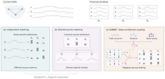
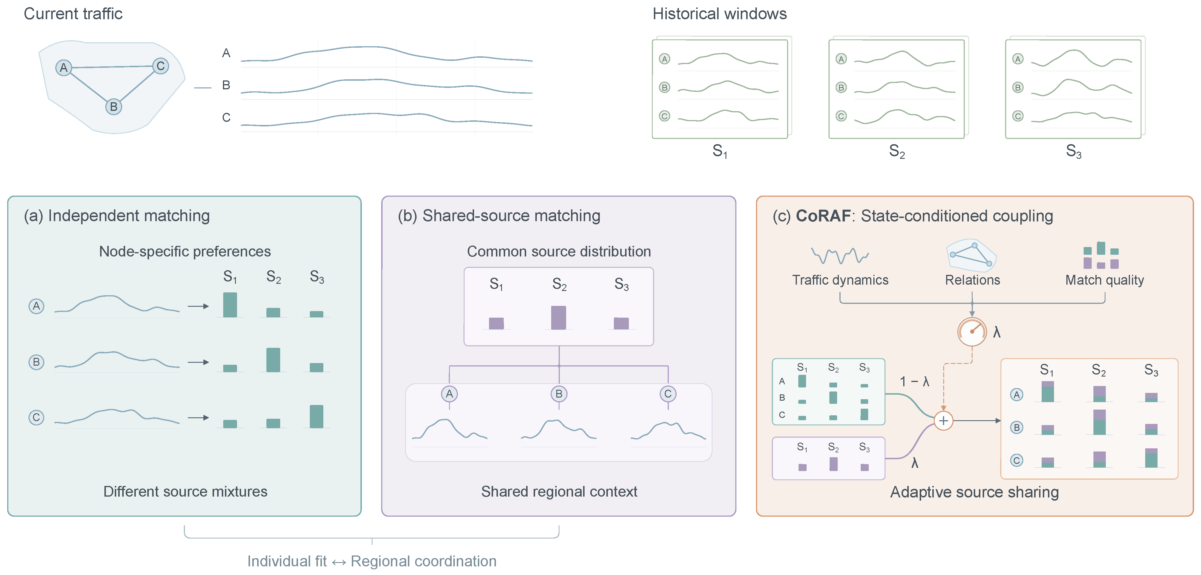
Figure 1 illustrates the tension between individual trajectory matching and shared historical context. Independent retrieval allows each node to select historical windows resembling its own trajectory, but related nodes may draw on different historical episodes, making the aggregated evidence less representative of their coordinated variation within a common historical context. Shared-source retrieval coordinates historical evidence through a common source distribution within each partition, but this distribution may provide a poorer match to local trajectories and smooth node-specific changes. Both effects matter for forecasting: the former can weaken cross-node coordination cues, whereas the latter can obscure local changes. As current fluctuations, inter-node relationships, and historical-match quality vary across input windows, the central question is how to balance local matching and cross-node source coordination for each forecast.
Figure 1.
Motivation for state-conditioned source coupling in traffic forecasting. The upper panels show current traffic at three connected nodes (A–C) and three historical source windows (–), each synchronized across nodes. (a) Independent matching assigns a node-specific distribution over historical sources. (b) Shared-source matching assigns a common distribution to nodes within a partition, coordinating their historical context. (c) CoRAF uses traffic dynamics, relation quality, and matching quality to determine the coupling coefficient . Teal and purple bar segments represent the independent and shared-source contributions, weighted by and , respectively. Curves and source weights are schematic.
We propose CoRAF, a retrieval-augmented forecasting framework that couples node-specific and partition-shared source distributions according to the current traffic state. The coupled historical input-window residual evidence and its observation coverage are encoded and integrated with the current traffic representation for multi-step prediction. We evaluate the framework on four real-world traffic datasets, using one hour of observations to forecast traffic flow over the following hour and provide predictive information for short-term traffic monitoring. The main technical contributions are as follows.
- Relation-guided historical retrieval. We construct node-specific and partition-shared source distributions over a common candidate pool. Trajectory similarity supports individual source preferences, while lagged inter-node relationships guide the selection of shared historical sources.
- State-conditioned source coupling. We learn a partition-level coefficient from traffic dynamics, relation quality, and matching quality. The same coefficient combines historical residual evidence and its observation coverage, adapting the contribution of shared sources to each input window.
2. Related Work
2.1. Spatio–Temporal Representation Learning for Traffic Forecasting
Spatio–temporal traffic forecasting models combine spatial interactions between sensors with the temporal evolution of their observations. STGCN [5] couples graph convolution with temporal convolution, whereas DCRNN [7] embeds bidirectional diffusion convolution within recurrent units. In multisensor forecasting, local measurements can also be summarized into a system-level indicator, as illustrated by the use of temperature readings to track bearing degradation [13]. STGCN and DCRNN use network connectivity to organize information exchange between nodes, with different mechanisms for accumulating temporal dependencies. In sensor networks, spatial dependencies can be learned from observations [14,15]. Graph WaveNet implements this idea through an adaptive adjacency matrix derived from node embeddings. These formulations establish spatial structure and temporal aggregation as two central design choices in traffic forecasting. STG-NCDE [16] uses two interacting controlled differential equations to model temporal evolution at individual sensors and spatial dependencies across the road network. When a forecaster draws evidence from multiple historical windows, a further question is how strongly related sensors should rely on the same historical episodes.
Attention-based sequence models can assign different weights to observations within the input window [17,18]. STAEformer introduces adaptive spatio–temporal embeddings into a Transformer architecture, allowing spatial and temporal attention to operate on representations that distinguish positions within the traffic sequence. HGCRN [19] uses spatio–temporal meta-embeddings to condition dynamic graph construction and graph-convolution parameters within recurrent modeling. These approaches address heterogeneity through different mechanisms: adaptive embeddings enrich the features processed by attention, while conditional parameter generation adjusts the transformations applied to traffic states. Both make spatial and temporal context explicit in representation learning.
Multiscale forecasting methods decompose a signal so that variations at different time scales can be modeled separately [20,21]. STWave uses wavelet decomposition to separate low- and high-frequency components and models their spatio–temporal dependencies through dedicated branches. HyperD [22] represents daily and weekly periodicity alongside a frequency-aware residual branch, with a dual-view alignment objective supporting component separation. DualCast [23] distinguishes intrinsic traffic patterns from representations associated with aperiodic events. RIFT-STGNN [24] combines mask-aware temporal–frequency encoding, multiple graph sources, and trend-aware temporal attention to represent short-window dynamics. These methods organize heterogeneous temporal information within the predictor. Memory- and retrieval-augmented forecasting extends this perspective by making stored traffic patterns explicitly accessible to the current forecasting query.
2.2. Memory- and Retrieval-Augmented Forecasting
Memory-augmented models provide reusable traffic representations through learned latent prototypes. MegaCRN [25] maintains a meta-node bank queried by node states and uses memory information to generate node embeddings for graph learning. DSTMAN [26] combines memory-guided adaptive graph construction with two-stage memory augmentation, incorporating stored latent patterns into forecasting representations. In these architectures, memory contents are trainable representations, and query-dependent reading determines which patterns contribute to the current state. Memory, therefore, serves both as a repository of learned traffic patterns and as a mechanism for adapting spatial or temporal representations.
Retrieval-based forecasting also accesses historical instances or encoded patterns associated with earlier observations. RAFT [11] retrieves historical input segments resembling the current query and uses their recorded continuation segments to support time-series prediction. This formulation links a current input pattern to concrete examples of subsequent evolution in the historical corpus. For traffic forecasting, RAST [27] maintains spatial and temporal vector stores, retrieves relevant latent patterns, and integrates the retrieved information with the current query through cross-attention. These approaches differ in the representation and temporal extent of their retrieval units, using historical trajectories or latent spatio–temporal patterns as forecasting context.
Historical prediction errors provide another form of retrievable evidence for forecast correction. DeCyReM [12] constructs queries from de-cycled representations and retrieves historical multi-horizon base-prediction errors selected for difficulty and diversity. A utility gate controls their contribution to the corrected forecast. MURECAST [28] ranks admissible historical error records by predicted correction utility and uses an empirically calibrated gate to determine correction activation. These methods organize retrieval around the usefulness of historical errors for adjusting an initial prediction. CoRAF focuses on the coordination of historical sources across nodes: it couples node-specific and partition-shared source distributions according to current traffic dynamics and matching quality. The coupled evidence consists of historical input-window residuals and is integrated into the forecasting representation.
3. Problem Definition
We represent a traffic sensor network as a graph , where contains N sensor nodes, describes their spatial connections, and is the adjacency matrix. Let denote the traffic flow at time t. Given an observation window of length L, the forecasting task is to estimate traffic flow over the following H time steps:
The input and target represent traffic flow in its original units. A measurement is valid when its value is finite and nonzero. Accordingly, the input observation mask and target observation mask are defined as
In the main experiments, we adopt a preprocessing convention that treats raw zero flow as missing. The input mask is computed from the raw observations and retained after imputation, while the target mask is computed independently from the raw targets for the training loss and validation and test evaluation. Validity is determined before standardization.
Historical input windows from the training period form a memory bank . The forecasting function uses the current observations, their validity information, the road graph, and historical evidence to produce a multistep prediction:
where denotes the trainable parameters. The learning objective is to minimize prediction error over valid target observations.
4. Methodology
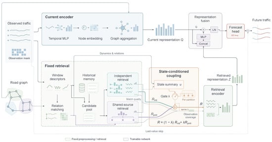
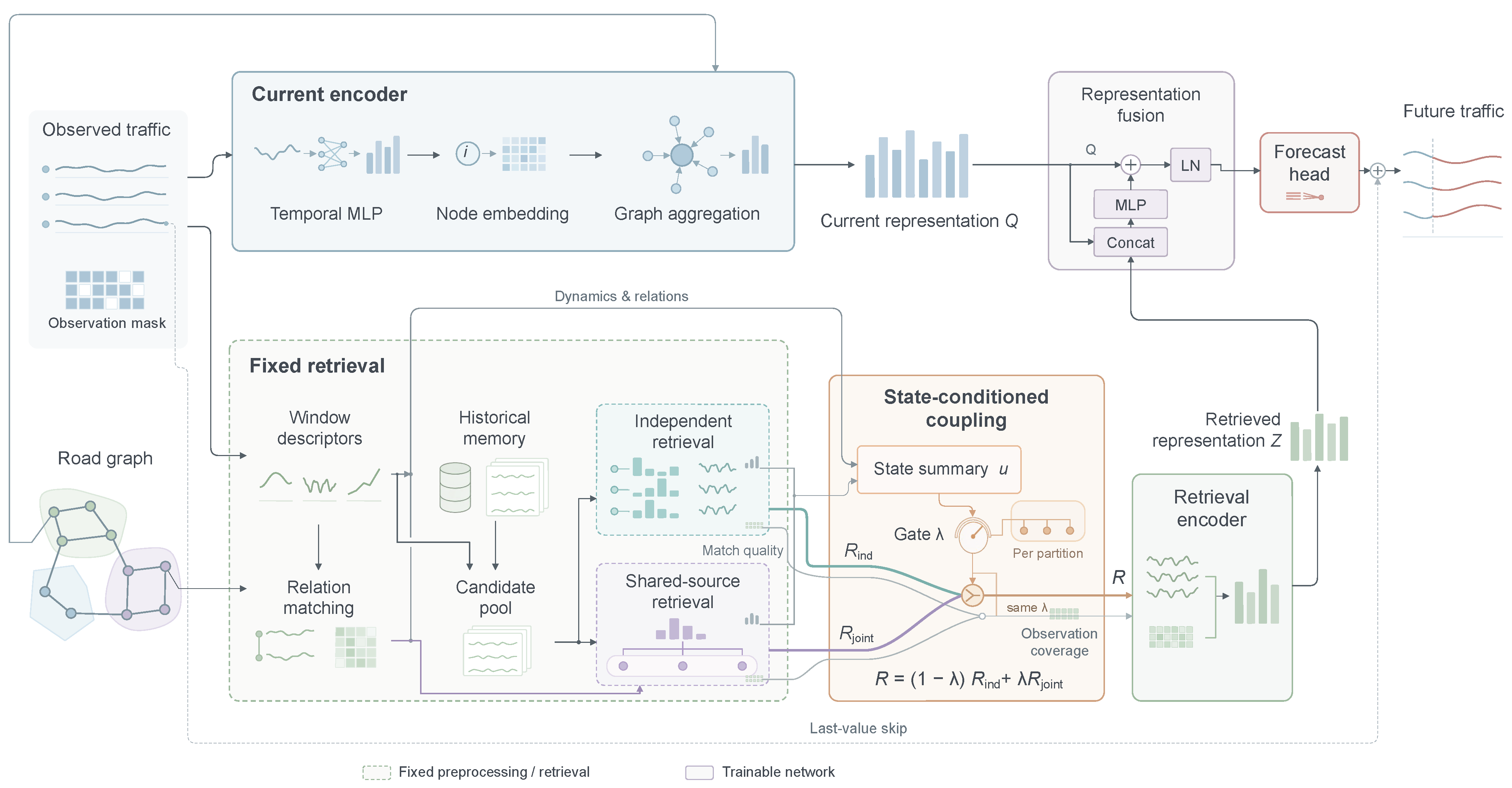
CoRAF formulates historical retrieval through two complementary aspects of a traffic window: the similarity of individual node trajectories and the compatibility of relations within a local region. Independent retrieval assigns a source distribution to each node, whereas shared-source retrieval assigns a common distribution to nodes within a partition. A state-conditioned gate controls their relative contributions using current traffic dynamics and retrieval quality. The resulting historical evidence is encoded together with its observation coverage and integrated with the current traffic representation for forecasting. Figure 2 illustrates the overall architecture.
Figure 2.
Overview of CoRAF. The current encoder produces representation Q. Fixed retrieval constructs independent and shared-source historical evidence, whose contributions are controlled by a state-conditioned gate. The coupled residuals and observation coverage are encoded into Z and fused with Q through a residual MLP. The forecasting head and last-value residual connection produce the standardized forecast.
We construct fixed, nonoverlapping graph partitions using deterministic breadth-first search. Each traversal starts from the lowest-index unassigned node and visits neighboring nodes in ascending index order, assigning up to S nodes to a partition. Each node is assigned once, and isolated nodes form singleton partitions. The resulting node sets satisfy
We denote the partition containing node i by , and its internal road edges by . These partitions define the scope of shared historical sourcing. For clarity, the query index t is omitted in the following derivations except where the forecasting origin or data split is required.
4.1. Current-Window Encoding
The current encoder captures the temporal evolution of traffic at each node and its spatial context. For each dataset, a global mean and population standard deviation are estimated from valid observations across all nodes in the training period. A positive lower bound is applied to the standard deviation for numerical stability. The same statistics are used to transform the training, validation, and test inputs.
The standardized input is completed by causal forward filling within each window. With , the filled sequence is defined recursively as
This initialization assigns the training mean to missing positions preceding the first valid observation. The original observation mask M is retained alongside . The current encoder and historical descriptor construction use these standardized, filled sequences and their observation masks.
At each temporal position ℓ, a linear projection embeds the flow value and its observation indicator. The projected sequence is flattened and processed by a temporal multilayer perceptron (MLP), after which a learnable node embedding is added:
Here, represents the identity of node i, and concatenates the temporal features into a vector. Because the input windows are sampled at a fixed interval, each position in the vector corresponds to a specific time lag. An MLP shared across sensors can, therefore, combine flow and observation-mask features at these lags directly, producing a representation of the current window for graph aggregation and fusion with historical evidence.
Spatial information is incorporated through graph aggregation:
where is the row-normalized adjacency matrix, with a self-connection assigned to isolated nodes. The aggregation follows the supplied road graph. Stacking the node representations gives the current representation , where d is the representation dimension.
4.2. Historical Memory and Window Descriptors
The historical memory stores synchronized input windows across the sensor network. Each source corresponds to a historical time interval and contains its residual trajectories, observation masks, and matching descriptors. Memory anchors are sampled at evenly spaced positions among training-window starts. The memory remains fixed during validation and testing. Let , , and denote the forecasting origins in the respective chronological splits. Each sample, including its input and target windows, lies within a single split. The eligible memory for a query at origin t is
Thus, training queries retrieve from historical windows that end before the query begins, while validation and test queries use the fixed training memory. Query and source windows undergo the same descriptor construction.
To characterize local fluctuations relative to the recent traffic level, we calculate an observation-weighted trailing background. Let , where w is the background window length. The background and residual are defined as
Two additional descriptors capture short-term changes and the average background level:
The first temporal difference is initialized to zero. A difference is valid for matching when both of its constituent observations are valid.
The node-level descriptor consists of the residual sequence, the first-difference sequence, and the average background. For node i and source s, let denote the distance for descriptor block a. Residual and difference distances are mean squared differences over jointly valid temporal positions; the background distance is the squared difference between the two background averages. Sequence blocks require sufficient observation overlap, and the background block requires sufficient observations in both windows. The combined distance is
where contains the available descriptor blocks, is a fixed block weight, and is a distance scale. An empty gives . Distance scales are estimated from positive valid distances between chronologically ordered training-memory pairs, using a median-based estimate with numerical stabilization.
4.3. Independent and Shared-Source Retrieval
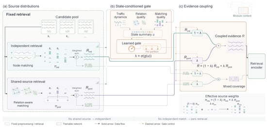
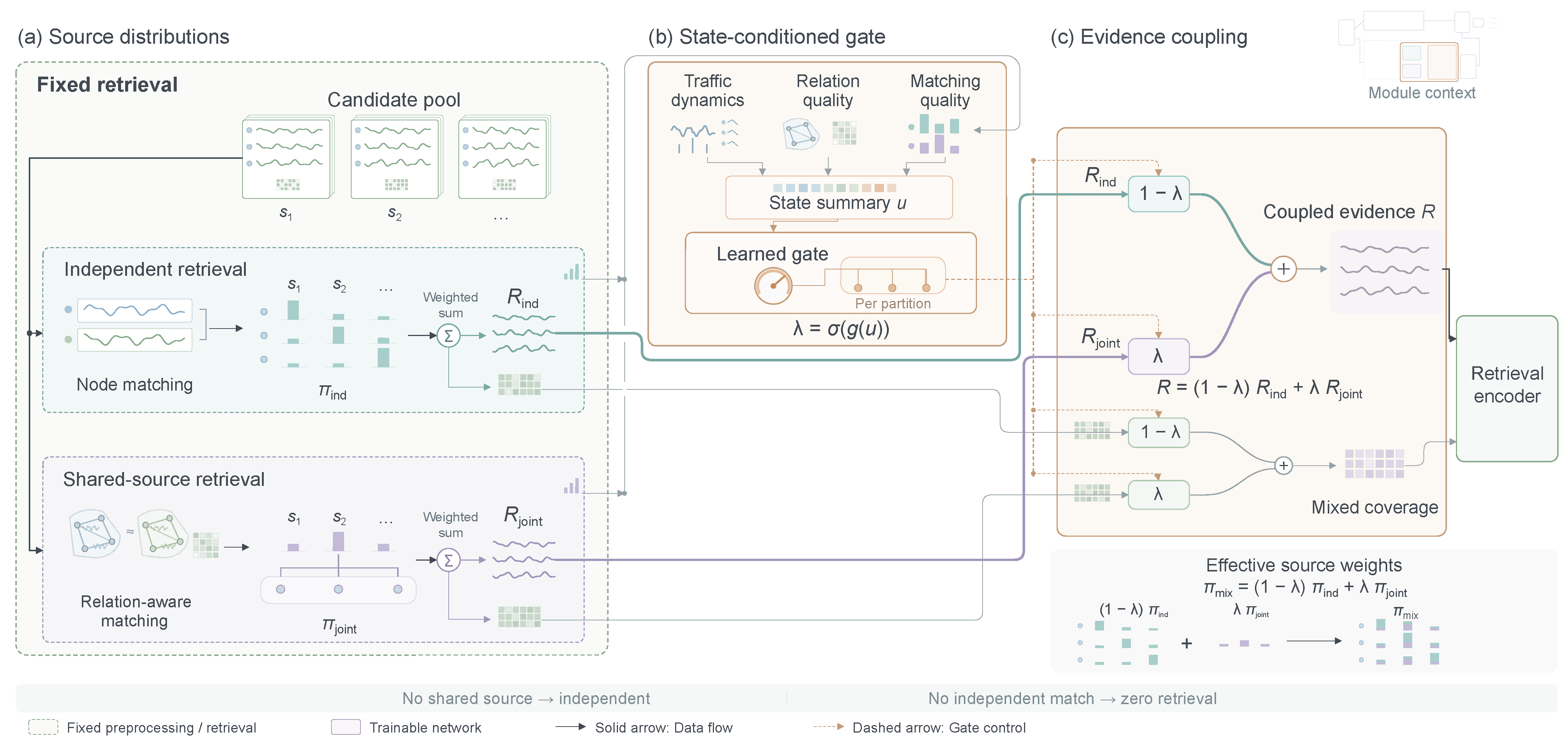
Figure 3 details the construction of source distributions and their subsequent state-conditioned coupling.
Figure 3.
Source distributions and state-conditioned coupling. (a) Independent and shared-source retrieval assign weights within a common candidate pool and aggregate historical residuals. Ellipses indicate additional candidate historical sources and their corresponding weight columns.(b) Traffic dynamics, relation quality, and matching quality form the state summary used by the gate. (c) The coupling coefficient mixes the residual evidence and its observation coverage before retrieval encoding.
- Candidate construction.
Candidate selection retains matches that are useful at either the node or partition level. For partition p and source , let be the set of comparable nodes. The partition-level distance is defined as
where specifies the required node coverage. Sources with finite partition-level distances form the eligible set used in candidate construction. The candidate pool is
Here, returns up to k sources with the smallest finite distances in . The union retains unique source identities.
- Relation matching.
Shared-source retrieval evaluates how well a historical window matches the local relation pattern. For an internal edge and lag k in a prescribed lag set , a relation descriptor is calculated from residual sequences:
where Corr is the Pearson correlation coefficient, contains aligned positions with valid observations at both nodes, , and controls shrinkage. A relation entry is valid when its observation overlap and residual variances meet the prescribed requirements.
Let contain the edge–lag coordinates that are valid in both the query and source s. Their relation distance is
where is estimated from training-memory pairs. A relation-eligible candidate satisfies the node-coverage requirement and . When the query has a valid relation profile and multiple candidates are relation-eligible, the relation indicator equals one, and the shared-source set consists of those candidates. Otherwise, and .
- Source distributions.
For node , let . Independent retrieval weights sources according to node-level distance. Shared-source retrieval uses the partition-level score :
Here, is the retrieval temperature and controls the contribution of relation matching. Weights outside the corresponding valid sets are zero, and an empty valid set yields a zero weight vector. The distribution varies across nodes, whereas is shared by nodes in the same partition.
Each distribution aggregates historical residuals and their observation masks using the same source weights:
The retrieved residuals and summarize historical fluctuations, while and quantify their weighted observation coverage. Source weights are applied consistently across the temporal positions of each historical window.
4.4. State-Conditioned Source Coupling
The contribution of shared historical sourcing is conditioned on the current traffic state and the quality of the available matches. For each partition, we construct a state summary
The first three components describe traffic dynamics. is the mean squared residual over valid observations, is the mean absolute first difference over valid consecutive observations, and is the standard deviation of node-wise mean absolute changes across nodes with valid differences. Relation quality is represented by the mean absolute valid relation coefficient and the fraction of valid edge–lag entries .
Matching quality is summarized by the expected distances under the two retrieval distributions. Let contain nodes with a nonempty independent source set. Then
Together with , these statistics describe the matching cost and the availability of relation-informed source selection. Empty summary sets receive zero-valued summaries.
The state summary is standardized using component-wise statistics estimated across training queries and partitions. A shared gating MLP maps the standardized state to a coupling coefficient:
where , is the sigmoid function, and is the gate network. The effective coefficient is shared by the nodes in partition p.
Let . The historical evidence and its coverage are coupled as
For an available node, this operation is equivalent to aggregating sources under the coupled weights
A smaller coefficient places greater weight on node-specific historical matches, while a larger coefficient increases the contribution of a common historical distribution. The same coefficient governs residual aggregation and observation coverage, preserving their correspondence in the coupled evidence.
4.5. Forecasting and Learning
The retrieval encoder converts the coupled historical evidence into a node representation. Let and . The encoder receives the residual sequence, its observation coverage, and source availability:
where denotes feature concatenation. The resulting representation Z supplies the forecasting network with both historical fluctuations and their observation support.
The current and retrieved representations are integrated through residual feature fusion:
The forecasting head predicts a horizon-specific residual relative to the final filled observation. Given the fused representation , the standardized forecast is
where is the final value of the standardized, filled input window and broadcasts this value across the forecasting horizon. The forecast is then transformed to the original traffic-flow units:
Collecting the node forecasts produces .
The model is trained using masked mean absolute error in the original traffic-flow units. Define the valid training-target indices as
The prediction objective is
This objective trains the current encoder, node embeddings, state-conditioned gate, retrieval encoder, fusion module, and forecasting head. Historical descriptors, candidate sets, base retrieval distributions, and state summaries are precomputed from the input windows. During optimization, the learned gate determines the contribution of historical evidence to each forecast.
5. Experiments
5.1. Experimental Setup
- Datasets and preprocessing. We evaluated CoRAF on four traffic-flow datasets from the California Performance Measurement System: PEMS03, PEMS04, PEMS07, and PEMS08. Their statistics are summarized in Table 1. All four datasets provide traffic observations at 5-min intervals. Each forecasting sample used the preceding 12 observations to predict the subsequent 12 observations, corresponding to a 60-min input window and a 60-min forecasting horizon. Each dataset was divided chronologically into training, validation, and test segments at a ratio of 6:2:2, with each complete input–target window contained within one segment. Traffic-flow values were standardized using a global mean and standard deviation estimated from valid observations in the training segment. Finite, nonzero raw observations were treated as valid. Missing inputs were filled causally within each window, using the training mean before the first valid observation. The historical memory was constructed from training input windows and held fixed during validation and testing.
Table 1.
Statistics of the four traffic datasets.
- Compared methods. We compared CoRAF with published results for 18 baseline configurations. Graph-based forecasting methods included STGCN [5], DCRNN [7], GWNet [14], ASTGCN [29], MTGNN [30], STGODE [31], DGCRN [32], and STPGNN [33]. ST-WA [34] and STICformer [35] represented attention-based approaches. Decomposition- and periodicity-based methods comprised D2STGNN [36], STWave [20], CycleNet-D and CycleNet-W [37], STDN [38], and HyperD [22]. DeCyReM [12] provided a retrieval-based comparison. Scores for 15 baseline configurations, including HyperD, were taken from Table 1 of the HyperD study [22]. STICformer and DeCyReM scores were taken from Tables 3 and 2 of their respective studies [12,35]. STG-NCDE scores were obtained from Table 3 of the original study [16]. These four source studies report a 6:2:2 training–validation–test split and a 12-step input window for predicting the following 12 steps. CoRAF results were obtained from our experiments. Published baseline scores retain the preprocessing, training, model-selection, and aggregation procedures of their source studies.
- Evaluation metrics. Forecasting accuracy was assessed using MAE, RMSE, and MAPE on the original traffic-flow scale. All three metrics used the same set of targets with finite, nonzero raw values. Errors were accumulated across all test samples, nodes, and 12 prediction steps and normalized by the total number of valid targets. MAE was the mean absolute error, and RMSE was the square root of the mean squared error. MAPE was computed over all valid targets as the mean ratio of absolute error to the absolute raw target value, multiplied by 100%. Lower values indicated better predictive performance for all three metrics.
- Implementation details. CoRAF was implemented in PyTorch 2.4.1 and trained on an NVIDIA GeForce RTX 4090 GPU. CoRAF and its five ablation variants were each trained independently using random seeds 42, 52, 62, 72, and 82 on all four datasets, yielding 120 runs. The data split, preprocessing pipeline, hyperparameters, and validation-based checkpoint-selection rule were held fixed across seeds. The hidden dimension was 64, the dropout rate was 0.1, and each graph partition contained at most eight nodes. Training used AdamW with an initial learning rate of , a weight decay of , and a batch size of 16 for a maximum of 100 epochs. The learning rate was halved after five consecutive epochs without improvement in validation MAE, with a minimum learning rate of . Early stopping used a patience of 20 epochs, and the gradient-clipping threshold was 5.0. The training objective was masked MAE computed on the original traffic-flow scale. The checkpoint achieving the lowest MAE over the complete validation set was selected for testing.
- Retrieval configuration. Both independent and shared-source retrieval used a temperature of . The relation-distance weight was , the correlation shrinkage parameter was , and the node- and relation-coverage thresholds were and , respectively. The causal background window contained five time steps. Candidate construction combined the valid top-ranked source from each node with the four highest-ranked valid sources at the partition level, retaining unique source identities with a candidate capacity of 12. When fewer valid sources were available, the available candidates were retained. The residual, first-difference, and average-background descriptor weights were 1, 1, and 0.1, respectively, with each distance block normalized using training-derived scales and evaluated under its validity mask.
- Gating configuration. The shared gating network comprised an eight-dimensional input, a fully connected layer with 32 units, a SiLU activation, and a scalar linear output followed by a sigmoid. The final linear layer’s weights and bias were initialized to zero, giving an initial sigmoid output of 0.5; the effective coupling coefficient followed the source-availability rules defined in Section 4.4. These retrieval and gating settings were fixed in advance in the implementation and used consistently across all four datasets and the complete-CoRAF runs in Section 5.2 and Section 5.3.
- Statistical analysis. Repeated-run performance was summarized as the mean and sample standard deviation across five runs, with each metric computed separately for each run before aggregation. The primary contrast was the mean test-MAE difference between Static Coupling and CoRAF, defined as Static Coupling minus CoRAF. We constructed dataset-specific 95% percentile confidence intervals using 10,000 paired moving-block bootstrap resamples of consecutive forecast origins. The primary block length was 24 h, with 12 h and 48 h used for sensitivity analysis. Each sampled block retained all nodes and all 12 prediction horizons, and identical temporal indices were used across models and seeds. Within each resample, MAE was recomputed over valid targets for each run, and the five paired differences were averaged. These intervals describe temporal uncertainty conditional on the five fitted model pairs and the observed network. Across-run standard deviations separately summarize training variability. Intervals were reported individually for each dataset. Section 5.2 reports CoRAF results from the run with random seed 42, whereas Section 5.3 summarizes five independent runs as the mean and sample standard deviation.
5.2. Overall Performance
Among the results listed in Table 2, CoRAF recorded the lowest values in 11 of the 12 dataset–metric comparisons, including MAE and MAPE on all four datasets. Its MAE values were 3.46%, 1.06%, and 6.29% below the published DeCyReM scores on PEMS03, PEMS04, and PEMS07, respectively. On PEMS08, CoRAF recorded an MAE of 13.23 compared with the published STICformer score of 13.29, a relative difference of 0.45%. The largest relative MAE difference occurred on PEMS07, where the respective values were 17.88 and 19.08.
Table 2.
Comparison with published benchmark results on four traffic-flow datasets. Baseline scores are taken from the HyperD, STICformer, DeCyReM, and STG-NCDE studies [12,16,22,35]. CoRAF scores are obtained from our experiments. Bold and underlined entries indicate the lowest and second-lowest reported values in each dataset–metric column, respectively. MAPE is reported as a percentage.
The reported RMSE rankings varied across datasets. CoRAF recorded the lowest listed RMSE on PEMS04, PEMS07, and PEMS08, with values of 29.20, 30.93, and 22.38, respectively. These values were 0.95%, 4.24%, and 2.14% below the lowest published baseline scores in the corresponding columns, reported by DeCyReM, STICformer, and DeCyReM, respectively. On PEMS03, CoRAF ranked third with an RMSE of 24.54, following DeCyReM at 23.31 and HyperD at 23.66. Thus, the published-score comparison showed a less uniform pattern for RMSE than for MAE and MAPE.
State-conditioned coupling adjusts the balance between node-specific and shared historical evidence using traffic dynamics, relation quality, and matching quality. Section 5.3 evaluates the contribution of this mechanism through comparisons with the corresponding CoRAF variants.
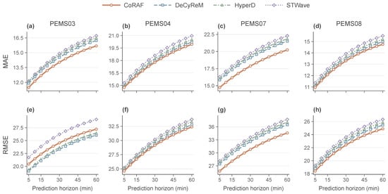
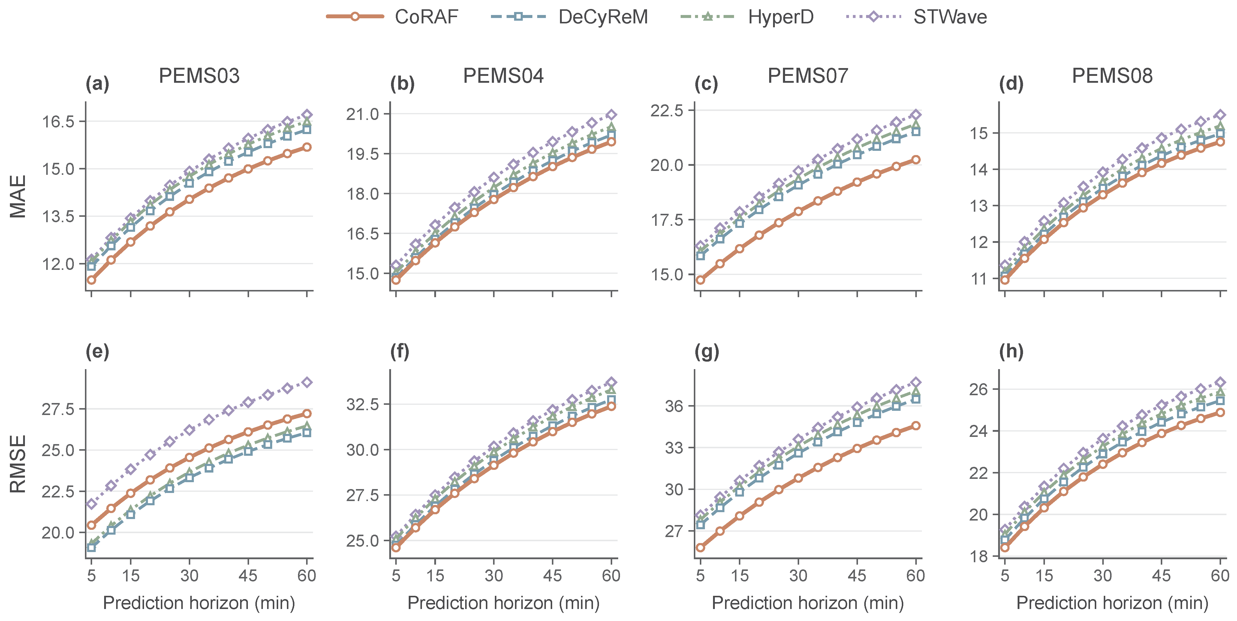
Figure 4 compares forecasting errors across the 12 prediction steps for CoRAF, DeCyReM, HyperD, and STWave. Errors increased with the prediction horizon for all four models. CoRAF maintained the lowest MAE at every prediction step on all four datasets, with a clear separation from the three baselines throughout the horizon on PEMS07. It also maintained the lowest RMSE across the prediction horizon on PEMS04, PEMS07, and PEMS08. On PEMS03, its RMSE remained above those of DeCyReM and HyperD and below that of STWave. The stepwise comparisons showed that the observed performance differences persisted across both short and long prediction horizons.
Figure 4.
Forecasting performance across prediction horizons. Panels (a–d) show MAE and panels (e–h) show RMSE on PEMS03, PEMS04, PEMS07, and PEMS08, respectively. Each curve reports errors at 12 prediction steps spanning 5–60 min. CoRAF results are from the run with random seed 42.
5.3. Ablation Study
Table 3 evaluates historical retrieval, source coupling, state conditioning, and relation-guided source selection across five random seeds. CoRAF achieved the lowest mean error in all 12 dataset–metric comparisons. Removing the encoded retrieval representation produced the largest mean-error increase among the five variants in every comparison. Mean MAE increased from 17.88 to 19.55 on PEMS07 and from 13.92 to 15.09 on PEMS03. These results support the contribution of historical residual evidence alongside the current input representation.
Table 3.
Ablation study across five random seeds on four datasets. (a,b) MAE, RMSE, and MAPE are reported as the mean ± sample standard deviation across five independent training runs. Bold entries indicate the lowest mean in each column. MAPE is expressed as a percentage. (c) Mean MAE differences, defined as Static Coupling minus CoRAF, and paired moving-block bootstrap 95% confidence intervals. The 24 h block is the primary analysis; 12 h and 48 h blocks assess sensitivity. Positive differences indicate lower MAE for CoRAF. Intervals are dataset-specific and conditional on the fitted models and observed network.
Independent Only and Shared-source Only fixed the coupling coefficient at zero and one, respectively, with the prescribed source-availability fallback. Independent Only achieved lower mean errors on PEMS03, PEMS04, and PEMS08, whereas Shared-source Only performed better on PEMS07 across all three metrics. On PEMS07, their mean MAE values were 18.61 and 18.36, respectively, compared with 17.88 for CoRAF. The relative performance of the two retrieval modes varied across datasets, while their state-conditioned combination achieved lower mean errors than either mode alone.
Static Coupling learned a separate scalar parameter for each partition and mapped it through a sigmoid to obtain the coupling coefficient. The coefficient was initialized to 0.5 and updated during training, while remaining constant across input windows for a given trained model. CoRAF achieved lower mean MAE, RMSE, and MAPE than this variant on all four datasets. Table 3c reports the paired MAE differences and their confidence intervals. The intervals remained above zero on PEMS03 and PEMS07 for all three block lengths, supporting lower MAE with state-conditioned coupling on these datasets. On PEMS04 and PEMS08, the mean differences favored CoRAF, but all three intervals included zero. The interval evidence, therefore, supported the MAE benefit on PEMS03 and PEMS07, while its direction remained uncertain on PEMS04 and PEMS08.
Removing relation-guided retrieval eliminated the relation-distance term and relation-based candidate eligibility screening while retaining the current relation features used by the gate. This variant had higher mean errors than CoRAF across all datasets and metrics. The largest mean MAE increase occurred on PEMS07, from 17.88 to 18.56. Relation-guided selection evaluates how historical windows reproduce the relationships between nodes, providing an additional criterion for selecting shared historical evidence.
Section 5.4 examines the contribution of each of the three gate input groups and evaluates how the choice of coupling coefficient and historical sources affects forecasting error.
5.4. Targeted Ablations of Gating and Retrieval
Table 4 reports the gating and retrieval ablations on PEMS04 and PEMS07. To assess the contribution of each gate input group, we separately set the standardized traffic-dynamics, relation-quality, or matching-quality components to zero during training and evaluation. When relation quality was removed from the gate, retrieval still used inter-node relations to select shared historical sources. Fixed Coupling set the raw coupling coefficient to 0.5. Random Gating drew a coefficient uniformly between zero and one for each query window and partition and reused it on subsequent visits. Random Retrieval sampled the same number of candidates as the original policy from historical windows satisfying the temporal and observation-validity criteria, assigned uniform weights within each eligible source set, and recomputed the gate state from the sampled sources. All variants used the same source-availability rules.
Table 4.
Ablations of gate inputs, coupling policies, and historical retrieval on PEMS04 and PEMS07. Results are reported as the mean ± sample standard deviation across random seeds 42, 52, and 62. MAPE is expressed as a percentage. Bold entries indicate the lowest mean in each column.
Removing any one of the three gate input groups increased mean MAE, RMSE, and MAPE on both datasets. Removing traffic dynamics produced the largest increase in mean MAE among the three input ablations, by 0.14 on PEMS04 and 0.44 on PEMS07. The other inputs differed in their relative contributions across datasets. On PEMS04, removing relation quality increased MAE more than removing matching quality (0.12 versus 0.07). On PEMS07, removing matching quality had the larger effect (0.29 versus 0.16).
The gating controls further distinguished the contributions of partition-specific and window-specific coefficients. Replacing the fixed coefficient of 0.5 with a learned constant for each partition reduced mean MAE from 18.05 to 18.00 on PEMS04 and from 18.55 to 18.37 on PEMS07. Conditioning the coefficient on the current window reduced mean MAE further, to 17.77 and 17.83, respectively. Random Gating yielded mean MAEs of 18.14 and 18.56. Random Retrieval produced the highest mean error for all three metrics on both datasets, with MAE exceeding that of CoRAF by 0.98 on PEMS04 and 1.57 on PEMS07. This result supports selecting and weighting historical sources according to match quality.
5.5. Coupling Behavior and Case Studies
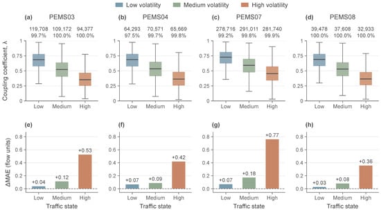
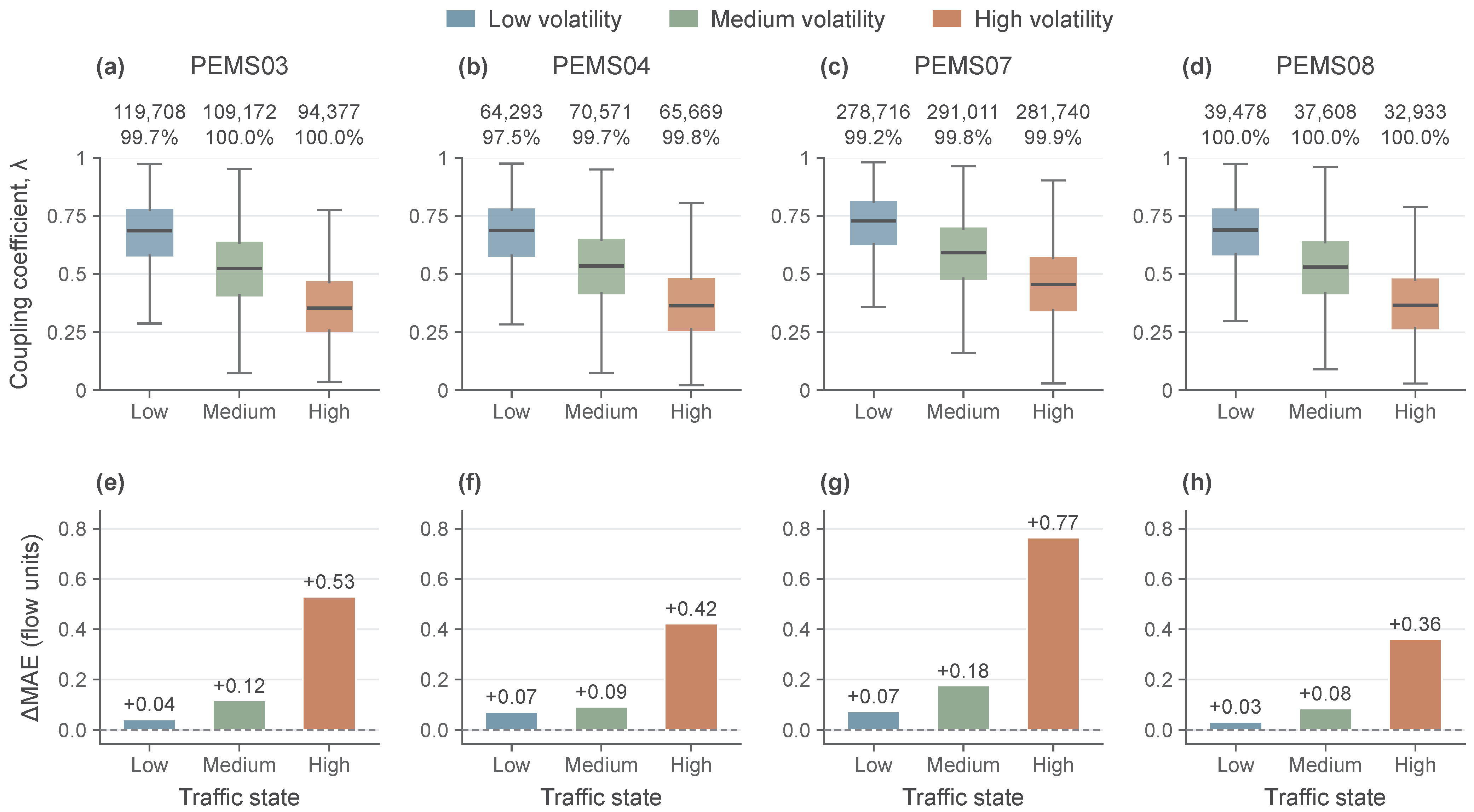
Figure 5 examines how source coupling varied with traffic volatility. We divided partition–window pairs into low-, medium-, and high-volatility groups using the 33rd and 67th percentiles of the traffic-change statistic estimated from each training set. Across all four datasets, the median coupling coefficient decreased as volatility increased. Among windows with available historical sources, the gate, therefore, assigned greater weight to shared-source evidence under low volatility and to node-specific evidence under high volatility. This pattern shows that the learned balance between the two retrieval distributions varied with the current traffic state.
Figure 5.
Coupling behavior and forecasting error across traffic states. Columns correspond to PEMS03, PEMS04, PEMS07, and PEMS08. Traffic states are defined using the training-set 33rd and 67th percentiles of . (a–d) Distributions of the coupling coefficient , which controls the contribution of shared-source evidence. Each box summarizes partition–window pairs with an available shared source and at least one valid independent match. Boxes span the 25th–75th percentiles, central lines indicate medians, and whiskers extend to the most extreme observations within 1.5 interquartile ranges of the box boundaries. The two annotation rows report the number of included partition–window pairs and the shared-source availability percentage within each state. (e–h) , aggregated over all valid prediction targets in each state. Positive values indicate lower errors for CoRAF. CoRAF and Static Coupling results are from runs with random seed 42.
In the run shown in Figure 5, the largest MAE difference between Static Coupling and CoRAF occurred in the high-volatility group. We measured this benefit as , using matched predictions and valid targets within each state. CoRAF achieved positive improvements in all three groups on every dataset. Under high volatility, MAE decreased by 0.53, 0.42, 0.77, and 0.36 on PEMS03, PEMS04, PEMS07, and PEMS08, respectively. The corresponding reductions under low volatility ranged from 0.03 to 0.07. These results locate the largest benefit of adaptive source weighting in windows with stronger traffic changes.
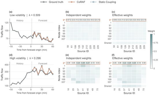
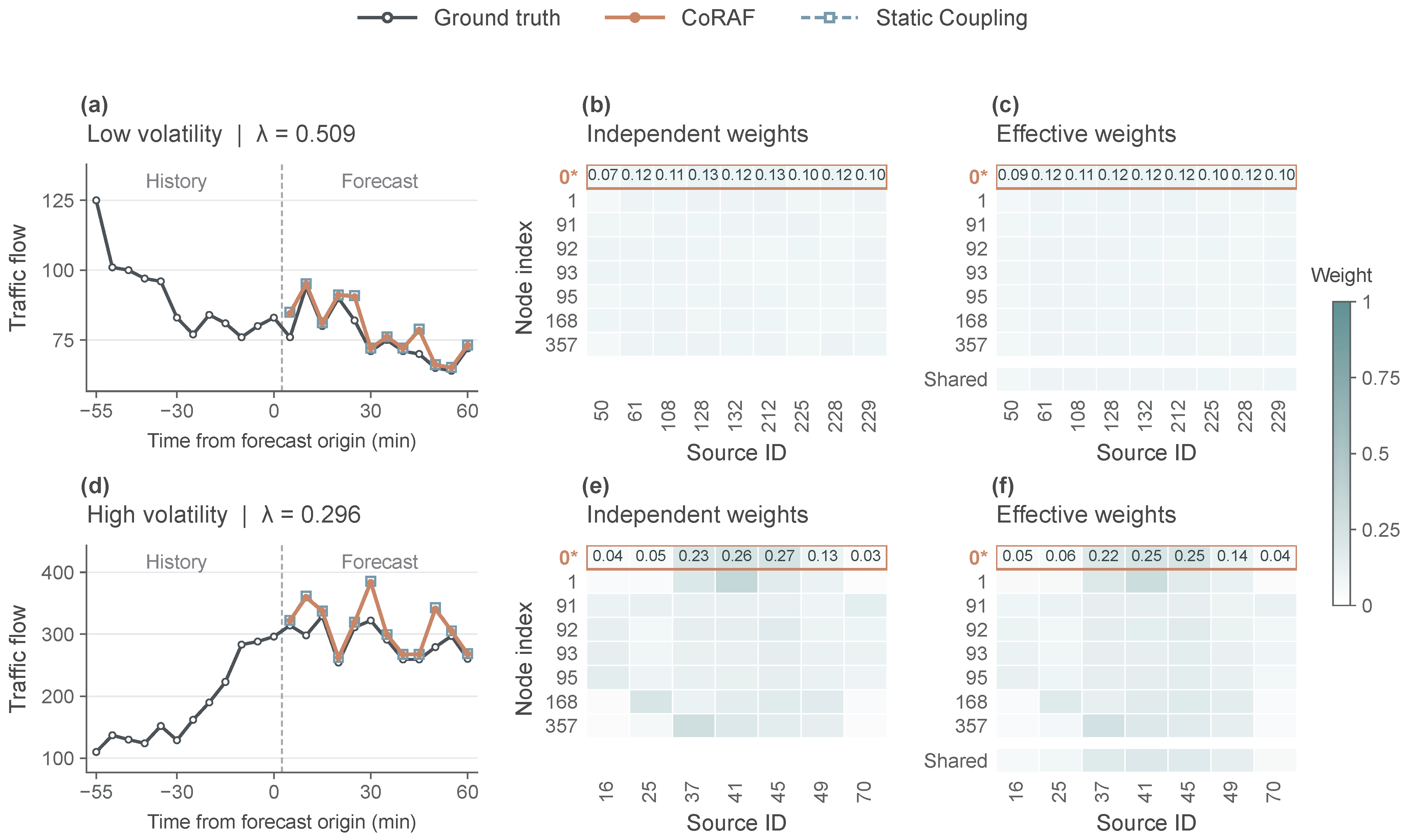
Figure 6 illustrates the source-weight adjustments for two windows from the same partition in PEMS07, with mapped node 0 used to display the forecasts. The coupling coefficient was 0.509 in the low-volatility case and 0.296 in the high-volatility case. For the displayed node, independent weights were relatively diffuse in the low-volatility window, whereas the high-volatility window assigned its largest weights to sources 37, 41, and 45. Coupling shifted these weights towards the shared distribution while preserving the dominant sources in the high-volatility case. CoRAF and Static Coupling produced similar forecast trajectories in these examples. The weight maps show how state-conditioned coupling adjusts historical-source contributions while preserving differences between nodes.
Figure 6.
Historical source weights and forecasting case studies. Two windows from the same partition in PEMS07 illustrate low-volatility (a–c) and high-volatility (d–f) conditions. (a,d) Twelve historical observations and twelve future observations, together with forecasts from CoRAF and Static Coupling for mapped node 0. Time is measured relative to the final input observation, and the vertical dashed line separates history from the forecasting interval. The corresponding coupling coefficient is shown above each panel. (b,e) Node-specific independent source weights. (c,f) Effective source weights after coupling, with the shared-source distribution shown beneath each heatmap. Source IDs follow the same column order within each case. In panels (b,c,e,f), the asterisk in the y-axis label 0* identifies mapped node 0, whose forecasts appear in panels (a,d). The orange outline highlights this node’s source weights; numerical annotations report its weights to two decimal places. All heatmaps share a common color scale. CoRAF and Static Coupling results are from runs with random seed 42.
5.6. Sensitivity Analysis
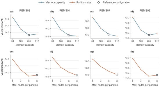
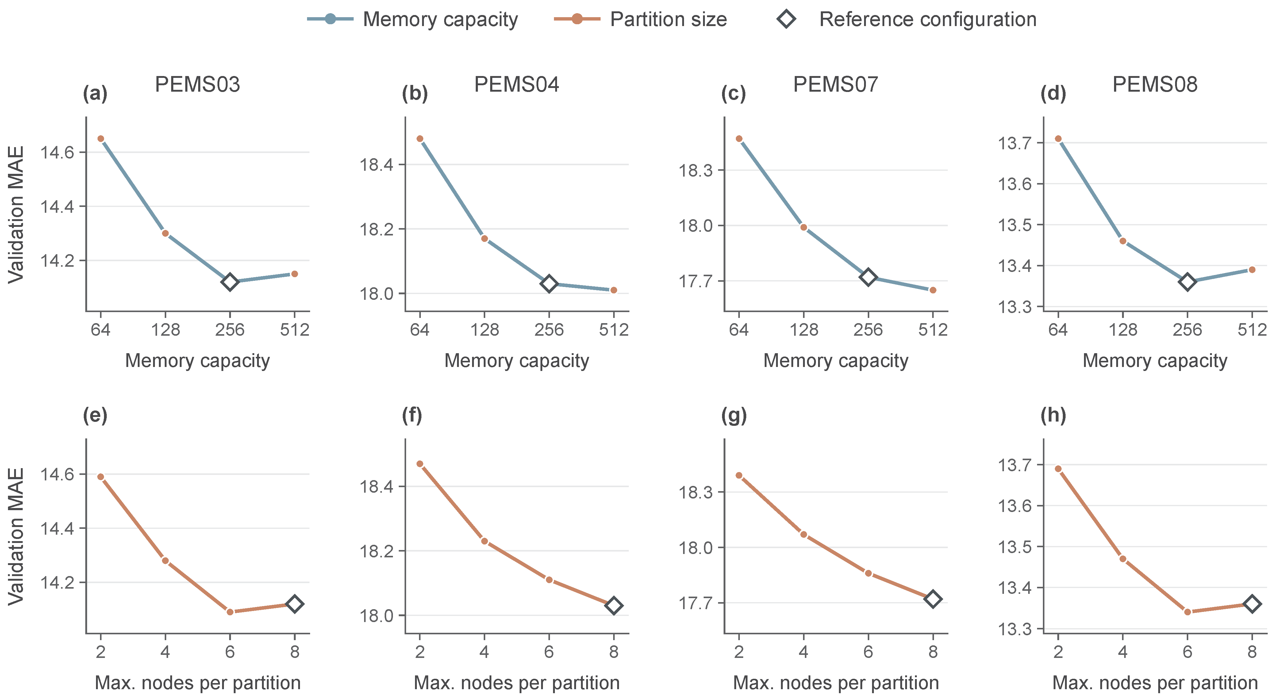
Figure 7 evaluates the sensitivity of CoRAF to memory capacity and partition size using validation MAE. We varied the number of historical windows in memory over , with the maximum partition size fixed at eight nodes. We then varied the maximum number of nodes per partition over , with memory capacity fixed at 256. The reference configuration used 256 historical windows and at most eight nodes per partition.
Figure 7.
Sensitivity to memory capacity and partition size. Columns correspond to PEMS03, PEMS04, PEMS07, and PEMS08. (a–d) Validation MAE for memory capacities of 64, 128, 256, and 512 historical windows, with a maximum of eight nodes per partition. (e–h) Validation MAE for maximum partition sizes of two, four, six, and eight nodes, with memory capacity fixed at 256. Other experimental settings are held constant within each sweep. Open diamonds indicate the reference configuration. Lower values indicate better performance. Each configuration was evaluated using random seed 42.
Increasing memory capacity from 64 to 256 reduced validation MAE on all four datasets, with the largest reduction occurring between 64 and 128. Expanding the memory to 512 produced smaller, dataset-dependent changes: PEMS04 and PEMS07 showed further reductions, whereas PEMS03 and PEMS08 showed slight increases. A larger memory expands the set of historical patterns available for matching. The curves indicate that most of the observed benefit was obtained within the range of 64–256 windows, with limited additional gains from further expansion.
Increasing the maximum partition size from two to six nodes also reduced validation MAE across all four datasets. PEMS04 and PEMS07 achieved their lowest errors at eight nodes, while PEMS03 and PEMS08 reached their minima at six nodes and showed a slight increase at eight. These minima indicate that the preferred spatial scope of shared-source retrieval varies across datasets.
5.7. Computational Cost
Computational costs were measured locally on an AMD Ryzen 9 7950X CPU with 64 GB RAM and an NVIDIA RTX 4090 GPU, using FP32 with AMP and TF32 disabled. PyTorch 2.4.1 intra-op and inter-op thread counts were eight and one, respectively; the DataLoader used four workers, and retrieval preprocessing used one BLAS thread. All models used the 6:2:2 split, 12-step input and prediction lengths, and a training batch size of 16. After one warm-up epoch, training time was averaged over five complete epochs, with CUDA synchronization at the timing boundaries. Each epoch included batch preparation, data transfer, forward and loss computation, backpropagation, gradient clipping, and optimizer updates. Measurements covered the training phase after preprocessing and retrieval-cache preparation.
Table 5a compares the parameter counts, per-epoch training times, and peak training GPU memory of CoRAF, HyperD, DeCyReM, and STWave on PEMS04 and PEMS07. CoRAF had the fewest parameters on both datasets, with 0.058 M parameters on PEMS04 and 0.095 M on PEMS07. Of these parameters, 10,368 belong to the temporal MLP shared across sensors and 321 to the source-coupling gate shared across partitions. Relative to HyperD, the smallest baseline in this comparison, these values corresponded to reductions of approximately 86.8% and 81.4%, respectively.
Table 5.
Computational cost on PEMS04 and PEMS07. (a) Parameter counts, mean training time per epoch, and peak training GPU memory from local measurements with batch size 16. CoRAF training uses precomputed retrieval inputs. Bold entries indicate the lowest value within each dataset. (b) CoRAF inference time in ms per complete-network query with batch size one, reported as mean ± sample standard deviation over 1500 timing records. End-to-end latency includes online retrieval, data transfers, network inference, and inverse normalization.
CoRAF also achieved the shortest per-epoch training times and the lowest peak training memory. Training required 6.4 s per epoch on PEMS04 and 21.2 s on PEMS07, corresponding to speedups of approximately and over HyperD. Peak training memory was 128 MiB and 384 MiB, respectively, compared with 972 MiB and 2472 MiB for HyperD. DeCyReM and STWave required more training time and memory on both datasets.
For CoRAF, fixed preparation took 1.84 s on PEMS04 and 4.92 s on PEMS07, covering raw-data and graph loading, preprocessing, partition and window-index generation, selection of 256 training-memory windows, fixed descriptor construction, distance-scale estimation, and state serialization. Subsequent query-cache construction took 58.60 s and 278.40 s for 16,923 and 28,155 queries, respectively, across the training, validation, and test splits. This stage reused the prepared memory and fitted the gating-state normalization statistics from training queries.
Table 5b reports CoRAF inference costs for a complete-network query with batch size one. After 100 warm-up executions, the first 500 valid test queries were evaluated chronologically in three rounds, yielding 1500 timing records per dataset. Each query performed retrieval against the loaded historical memory. Retrieval timing covered CPU input processing through construction of the retrieval tensors and standardized gating state; network timing covered the GPU forward pass. End-to-end latency was measured independently from a CPU-resident raw input window to the original-scale prediction returned to the CPU, including retrieval, transfers, and inverse normalization. GPU timing boundaries were synchronized. The maximum absolute prediction differences between online and cached retrieval were 0.000122 and 0.000244 in original flow units on PEMS04 and PEMS07, respectively. Retrieval accounted for most of the measured query-time cost.
5.8. Sensitivity to Zero-Value Handling
We assessed CoRAF’s sensitivity to raw zero-value handling by comparing two policies: the main policy treated zeros as missing, whereas the alternative retained all finite observations, including zeros, as valid. For each dataset, the alternative policy was trained independently using random seed 42 with the remaining hyperparameters and training procedure unchanged. Under the alternative validity rule, we recomputed training-derived normalization statistics and rebuilt the imputed inputs, historical-memory descriptors, retrieval caches, relation-validity masks, gate-state normalization statistics, and training-target masks. Both policies used the same finite, nonzero target sets for validation-based checkpoint selection and test evaluation.
Table 6 reports the results of both policies. Retaining zeros changed MAE by to across the four datasets, with a maximum absolute relative change of 1.51% across all 12 dataset–metric combinations. PEMS04 showed the largest error increases, whereas MAE and MAPE on PEMS07 and MAPE on PEMS08 decreased slightly. These paired runs showed modest changes in forecasting errors under the common nonzero-target evaluation, with the direction varying across datasets and metrics.
Table 6.
Sensitivity of CoRAF to zero-value handling on four traffic-flow datasets. Each policy used random seed 42. Both policies used the same finite, nonzero target sets for validation-based checkpoint selection and test evaluation. Each cell reports MAE, RMSE, and MAPE (%), respectively.
6. Discussion and Conclusions
This study examined how historical source sharing should adapt to heterogeneous traffic states. Across four PeMS datasets, CoRAF achieved the lowest reported MAE and MAPE among the compared methods, with RMSE gains varying across datasets. The ablations and state analyses support treating source sharing as a choice that varies with traffic state: individual and shared evidence contributed differently across datasets, and adaptive coupling yielded larger improvements over static coupling under high volatility.
RAFT [11] and DeCyReM [12] illustrate the value of retrieving historical continuations and prediction errors, respectively. CoRAF adds a complementary perspective by regulating coordination among the source distributions used by related sensors. These results support considering both match relevance and cross-node source coordination when organizing historical evidence.
The resulting one-hour flow forecasts can support anticipation of short-term demand changes and prioritization of traffic monitoring. With precomputed retrieval inputs, CoRAF required less time per training epoch and lower peak training GPU memory than the evaluated baselines on PEMS04 and PEMS07. The inference measurements additionally account for query-time retrieval and data transfer, with retrieval contributing most of the measured latency.
The fixed training memory and graph partitions constrain the coverage of historical patterns and the spatial scope of shared sourcing. Comparing chronological memory updates and selective retention would test the value of renewing historical evidence under changing traffic patterns. Dataset-dependent partition-size optima also motivate comparisons with adaptive or multiscale grouping. These studies would clarify how source coordination should evolve as traffic patterns and network conditions change. Interactions between sensing modalities can reveal complementary features of a road scene [39]. These features could provide additional context for selecting historical traffic windows. Future work could evaluate traffic-speed forecasting on METR-LA and PEMS-BAY to assess the applicability of state-conditioned source coupling across traffic variables. Speed forecasts could also inform downstream applications such as vehicle emission estimation, where the effect of speed varies with road gradient [40].
Author Contributions
Conceptualization, Z.W.; methodology, Z.W.; software, Z.W.; validation, Z.W., C.S. and J.Z.; formal analysis, Z.W.; investigation, Z.W.; data curation, Z.W. and C.S.; writing—original draft preparation, Z.W.; writing—review and editing, Z.W., C.S. and J.Z.; visualization, Z.W. and J.Z.; project administration, Z.W. All authors have read and agreed to the published version of the manuscript.
Funding
This research received no external funding.
Data Availability Statement
The raw PeMS traffic datasets used in this study are openly available in the Caltrans Performance Measurement System at https://pems.dot.ca.gov/, accessed on 1 July 2026. The processed data splits, configuration files, and experimental logs that support the findings of this study are available from the corresponding author upon reasonable request. The source code and implementation details are also available from the corresponding author upon reasonable request.
Conflicts of Interest
The authors declare no conflicts of interest.
References
- Yu, Q.; Yang, Y.; Xiong, X.; Sun, S.; Liu, Y.; Wang, Y. Assessing the impact of multi-dimensional driving behaviors on link-level emissions based on a Portable Emission Measurement System (PEMS). Atmos. Pollut. Res. 2021, 12, 414–424. [Google Scholar] [CrossRef] [Scilit]
- Jiang, J.; Han, C.; Zhao, W.X.; Wang, J. PDFormer: Propagation Delay-Aware Dynamic Long-Range Transformer for Traffic Flow Prediction. Proc. Aaai Conf. Artif. Intell. 2023, 37, 4365–4373. [Google Scholar] [CrossRef] [Scilit]
- Cheng, G.; Guo, L.; Zhang, T. Spatial Equity Assessment of Bus Travel Behavior for Pilgrimage: Evidence from Lhasa, Tibet, China. Sustainability 2022, 14, 10486. [Google Scholar] [CrossRef] [Scilit]
- Jia, Q.; Zhang, T.; Cheng, L.; Cheng, G.; Jin, M. The Impact of the Neighborhood Built Environment on the Walking Activity of Older Adults: A Multi-Scale Spatial Heterogeneity Analysis. Sustainability 2022, 14, 13927. [Google Scholar] [CrossRef] [Scilit]
- Yu, B.; Yin, H.; Zhu, Z. Spatio-Temporal Graph Convolutional Networks: A Deep Learning Framework for Traffic Forecasting. In Proceedings of the Twenty-Seventh International Joint Conference on Artificial Intelligence, Stockholm, Sweden, 13–19 July 2018; pp. 3634–3640. [Google Scholar] [CrossRef] [Scilit] [PubMed]
- Bai, L.; Yao, L.; Li, C.; Wang, X.; Wang, C. Adaptive Graph Convolutional Recurrent Network for Traffic Forecasting. In Proceedings of the 34th Annual Conference on Neural Information Processing Systems (NeurIPS 2020), Virtual Event, 6–12 December 2020; Volume 33, pp. 17804–17815. [Google Scholar]
- Li, Y.; Yu, R.; Shahabi, C.; Liu, Y. Diffusion Convolutional Recurrent Neural Network: Data-Driven Traffic Forecasting. In Proceedings of the 6th International Conference on Learning Representations (ICLR 2018), Vancouver, BC, Canada, 30 April–3 May 2018. [Google Scholar]
- Cui, Q.; Ding, Z.; Chen, F. Hybrid Directed Hypergraph Learning and Forecasting of Skeleton-Based Human Poses. Cyborg Bionic Syst. 2024, 5, 0093. [Google Scholar] [CrossRef] [Scilit] [PubMed]
- Deng, J.; Chen, X.; Jiang, R.; Song, X.; Tsang, I.W. ST-Norm: Spatial and Temporal Normalization for Multi-variate Time Series Forecasting. In Proceedings of the 27th ACM SIGKDD Conference on Knowledge Discovery & Data Mining, Virtual Event, Singapore, 14–18 August 2021; pp. 269–278. [Google Scholar] [CrossRef] [Scilit]
- Xie, Q.; Jiang, Y.; Xu, J.; Zhang, Y. ST-FGDIR: Spatiotemporal Traffic Forecasting with Forecast-Gain-Guided Deviation–Invariance Routing. Sensors 2026, 26, 6319. [Google Scholar] [CrossRef] [Scilit] [PubMed]
- Han, S.; Lee, S.; Cha, M.; Arik, S.O.; Yoon, J. Retrieval Augmented Time Series Forecasting. In Proceedings of the 42nd International Conference on Machine Learning, Vancouver, BC, Canada, 13–19 July 2025; Volume 267, pp. 21774–21797. [Google Scholar]
- Xie, Q.; Xu, J.; Lu, Y.; Zhang, Y. DeCyReM: De-Cycled Residual Memory with Utility-Gated Retrieval for Traffic Flow Forecasting. Mathematics 2026, 14, 3207. [Google Scholar] [CrossRef] [Scilit]
- Liu, M.; Dong, Z.; Shi, H. Multi-Sensor Information Fusion and Multi-Model Fusion-Based Remaining Useful Life Prediction of Fan Slewing Bearings with the Nonlinear Wiener Process. Sustainability 2023, 15, 12010. [Google Scholar] [CrossRef] [Scilit]
- Wu, Z.; Pan, S.; Long, G.; Jiang, J.; Zhang, C. Graph WaveNet for Deep Spatial-Temporal Graph Modeling. In Proceedings of the Twenty-Eighth International Joint Conference on Artificial Intelligence, Macao, China, 10–16 August 2019; pp. 1907–1913. [Google Scholar] [CrossRef] [Scilit] [PubMed]
- Ye, W.; Wang, J.; Chen, L.; Dai, L.; Sun, Z.; Liang, Z. Adaptive Spatial–Temporal Aware Graph Learning for EEG-Based Emotion Recognition. Cyborg Bionic Syst. 2024, 5, 0088. [Google Scholar] [CrossRef] [Scilit] [PubMed]
- Choi, J.; Choi, H.; Hwang, J.; Park, N. Graph Neural Controlled Differential Equations for Traffic Forecasting. Proc. Aaai Conf. Artif. Intell. 2022, 36, 6367–6374. [Google Scholar] [CrossRef] [Scilit]
- Liu, H.; Dong, Z.; Jiang, R.; Deng, J.; Deng, J.; Chen, Q.; Song, X. Spatio-Temporal Adaptive Embedding Makes Vanilla Transformer SOTA for Traffic Forecasting. In Proceedings of the 32nd ACM International Conference on Information and Knowledge Management, Birmingham, UK, 21–25 October 2023; pp. 4125–4129. [Google Scholar] [CrossRef] [Scilit]
- Han, Z.; Tian, H.; Han, X.; Wu, J.; Zhang, W.; Li, C.; Qiu, L.; Duan, X.; Tian, W. A Respiratory Motion Prediction Method Based on LSTM-AE with Attention Mechanism for Spine Surgery. Cyborg Bionic Syst. 2024, 5, 0063. [Google Scholar] [CrossRef] [Scilit] [PubMed]
- Xie, Q.; Xu, J.; Xie, X. Heterogeneity-aware graph convolutional recurrent network for traffic forecasting. AIP Adv. 2025, 15, 125033. [Google Scholar] [CrossRef] [Scilit]
- Fang, Y.; Qin, Y.; Luo, H.; Zhao, F.; Xu, B.; Zeng, L.; Wang, C. When Spatio-Temporal Meet Wavelets: Disentangled Traffic Forecasting via Efficient Spectral Graph Attention Networks. In Proceedings of the 2023 IEEE 39th International Conference on Data Engineering (ICDE), Anaheim, CA, USA, 3–7 April 2023; pp. 517–529. [Google Scholar] [CrossRef] [Scilit]
- Chen, H.; Li, Z.; Liu, J.; Hu, C.; Li, Z.; Cui, J. Multi-Scale ICEEMDAN–VMD Decomposition and Optimization-Enhanced CNN–BiGRU-MHA Model for ECT Accuracy Forecasting. Cybern. Syst. 2026, 57, 2026–2057. [Google Scholar] [CrossRef] [Scilit]
- Shao, M.; Zhang, Z.; Wang, Y.; Dai, Y.; Shen, X.; Wang, X. HyperD: Hybrid Periodicity Decoupling Framework for Traffic Forecasting. Proc. Aaai Conf. Artif. Intell. 2026, 40, 15689–15697. [Google Scholar] [CrossRef] [Scilit]
- Su, X.; Liu, F.; Chang, Y.; Tanin, E.; Sarvi, M.; Qi, J. DualCast: A Model to Disentangle Aperiodic Events from Traffic Series. In Proceedings of the Thirty-Fourth International Joint Conference on Artificial Intelligence, Montreal, Canada, 16–22 August 2025; pp. 3290–3298. [Google Scholar] [CrossRef] [Scilit] [PubMed]
- Xie, Q.; Xu, J.; Lu, Y.; Zhang, Y. RIFT-STGNN: Robust Interleaved Frequency–Trend Spatio-Temporal Graph Neural Network for Traffic Flow Forecasting. Mathematics 2026, 14, 2670. [Google Scholar] [CrossRef] [Scilit]
- Jiang, R.; Wang, Z.; Yong, J.; Jeph, P.; Chen, Q.; Kobayashi, Y.; Song, X.; Fukushima, S.; Suzumura, T. Spatio-Temporal Meta-Graph Learning for Traffic Forecasting. Proc. Aaai Conf. Artif. Intell. 2023, 37, 8078–8086. [Google Scholar] [CrossRef] [Scilit]
- Zhang, H.; Xie, Q.; Shou, Z.; Gao, Y. Dynamic Spatial-Temporal Memory Augmentation Network for Traffic Prediction. Sensors 2024, 24, 6659. [Google Scholar] [CrossRef] [Scilit] [PubMed]
- Ruan, W.; Dang, X.; Zhou, Z.; Lyu, S.; Liang, Y. A Retrieval Augmented Spatio-Temporal Framework for Traffic Prediction. Proc. Aaai Conf. Artif. Intell. 2026, 40, 39163–39172. [Google Scholar] [CrossRef] [Scilit]
- Jin, X.; Xu, J.; Xie, Q.; Zhang, Y. MURECAST: Memory-Based Utility-Aligned Residual Evidence with Calibrated Activation for Selective Correction of Traffic-Flow Forecasts. Symmetry 2026, 18, 1485. [Google Scholar] [CrossRef] [Scilit]
- Guo, S.; Lin, Y.; Feng, N.; Song, C.; Wan, H. Attention Based Spatial-Temporal Graph Convolutional Networks for Traffic Flow Forecasting. Proc. Aaai Conf. Artif. Intell. 2019, 33, 922–929. [Google Scholar] [CrossRef] [Scilit]
- Wu, Z.; Pan, S.; Long, G.; Jiang, J.; Chang, X.; Zhang, C. Connecting the Dots: Multivariate Time Series Forecasting with Graph Neural Networks. In Proceedings of the 26th ACM SIGKDD International Conference on Knowledge Discovery & Data Mining, Virtual Event, 23–27 August 2020; pp. 753–763. [Google Scholar] [CrossRef] [Scilit]
- Fang, Z.; Long, Q.; Song, G.; Xie, K. Spatial-Temporal Graph ODE Networks for Traffic Flow Forecasting. In Proceedings of the 27th ACM SIGKDD Conference on Knowledge Discovery & Data Mining, Virtual Event, Singapore, 14–18 August 2021; pp. 364–373. [Google Scholar] [CrossRef] [Scilit]
- Li, F.; Feng, J.; Yan, H.; Jin, G.; Yang, F.; Sun, F.; Jin, D.; Li, Y. Dynamic Graph Convolutional Recurrent Network for Traffic Prediction: Benchmark and Solution. ACM Trans. Knowl. Discov. Data 2023, 17, 9:1–9:21. [Google Scholar] [CrossRef] [Scilit]
- Kong, W.; Guo, Z.; Liu, Y. Spatio-Temporal Pivotal Graph Neural Networks for Traffic Flow Forecasting. Proc. Aaai Conf. Artif. Intell. 2024, 38, 8627–8635. [Google Scholar] [CrossRef] [Scilit]
- Cirstea, R.G.; Yang, B.; Guo, C.; Kieu, T.; Pan, S. Towards Spatio-Temporal Aware Traffic Time Series Forecasting. In Proceedings of the 2022 IEEE 38th International Conference on Data Engineering (ICDE), Virtual Event, 9–12 May 2022; pp. 2900–2913. [Google Scholar] [CrossRef] [Scilit]
- Chu, Y.; Fu, T.; Liu, P.; Lao, H. STICformer: Spatio-temporal intrinsic connections transformer for traffic flow prediction. Sci. Rep. 2026, 16, 1881. [Google Scholar] [CrossRef] [Scilit] [PubMed]
- Shao, Z.; Zhang, Z.; Wei, W.; Wang, F.; Xu, Y.; Cao, X.; Jensen, C.S. Decoupled dynamic spatial-temporal graph neural network for traffic forecasting. Proc. Vldb Endow. 2022, 15, 2733–2746. [Google Scholar] [CrossRef] [Scilit]
- Lin, S.; Lin, W.; Hu, X.; Wu, W.; Mo, R.; Zhong, H. CycleNet: Enhancing Time Series Forecasting through Modeling Periodic Patterns. In Proceedings of the 38th Annual Conference on Neural Information Processing Systems (NeurIPS 2024), Vancouver, BC, Canada, 10–15 December 2024; Volume 37, pp. 106315–106345. [Google Scholar] [CrossRef] [Scilit]
- Cao, L.; Wang, B.; Jiang, G.; Yu, Y.; Dong, J. Spatiotemporal-aware Trend-Seasonality Decomposition Network for Traffic Flow Forecasting. Proc. Aaai Conf. Artif. Intell. 2025, 39, 11463–11471. [Google Scholar] [CrossRef] [Scilit]
- Liu, X.; Li, Z.; Zhou, Y.; Peng, Y.; Luo, J. Camera–Radar Fusion with Modality Interaction and Radar Gaussian Expansion for 3D Object Detection. Cyborg Bionic Syst. 2024, 5, 0079. [Google Scholar] [CrossRef] [Scilit] [PubMed]
- Yang, Y.; Hou, J.; Yu, Q.; Zhang, T. Exploring the interactive effects of speed and slope on pollutant emissions from light-duty vehicles based on big data. Atmos. Pollut. Res. 2026, 17, 102962. [Google Scholar] [CrossRef] [Scilit]

Disclaimer/Publisher’s Note: The statements, opinions and data contained in all publications are solely those of the individual author(s) and contributor(s) and not of MDPI and/or the editor(s). MDPI and/or the editor(s) disclaim responsibility for any injury to people or property resulting from any ideas, methods, instructions or products referred to in the content. |
© 2026 by the authors. Licensee MDPI, Basel, Switzerland. This article is an open access article distributed under the terms and conditions of the Creative Commons Attribution (CC BY) license.