


Abstract
Annual maximum data are frequently recorded as integers, yet they are routinely modeled with the continuous generalized extreme value (GEV) distribution. We study the discrete GEV distribution of Dkengne et al. (2016), which is the distribution of the integer part of a continuous GEV random variable, and we provide a systematic treatment of its distributional, inferential and finite-sample properties. The model retains the location, scale and shape parameters of its continuous counterpart and contains the discrete Gumbel, discrete Fréchet and discrete (reversed) Weibull distributions as particular cases. We give the support (including the endpoint cases), the probability mass and cumulative distribution functions, their tail behavior, moments, the quantile function, and quantile-based measures of skewness and kurtosis. For maximum likelihood estimation, we identify the subsets of the parameter space on which the support is locally fixed, show that the model is differentiable in quadratic mean on a larger set that also contains integer endpoints when , and state the resulting asymptotic normality. We also show that flooring, ceiling and rounding of a GEV variable all lead to the same discrete family up to a shift in location. Simulation studies examine the finite-sample performance of the estimators and compare the discrete GEV with the continuous GEV fitted to the integer values under several observation mechanisms, including block maxima of integer counts. Applications to annual maximum wind speeds at Lisbon and annual maximum temperatures at Oxford are analyzed with discrete versions of the Kolmogorov–Smirnov, Cramér–von Mises and Anderson–Darling statistics calibrated by a parametric bootstrap.
Keywords:
annual maximum data; generalized extreme value distribution; maximum likelihood estimates; discrete extreme value distributions; goodness of fit for discrete data MSC:
62E99
1. Introduction
The Generalized Extreme Value (GEV) distribution is a family of continuous probability distributions that arises in the modeling of extreme values, such as the maximum or minimum of a large set of independent random variables. It is grounded in extreme value theory, a branch of statistics that focuses on understanding the behavior of the tails of distributions. The GEV distribution unifies three distinct types of extreme value distributions—the Gumbel, Fréchet and (reversed) Weibull—into a single parametric framework. Its flexibility makes it a popular choice in fields such as hydrology, finance, environmental science, and engineering, where the prediction of rare events, such as floods, market crashes, or structural failures, is critical.
The GEV distribution can be specified by the cumulative distribution function (Fisher and Tippett [1]; Gnedenko [2]; Jenkinson [3])
for if , if and if , where denotes a location parameter, denotes a scale parameter and denotes a shape parameter. Note that if X has distribution function (1) and , then X has a heavy tail bounded below by . If , then X has a short tail bounded above by .
The GEV distribution has been extensively used for modeling block maxima. Recent applications include analysis of a stationary climatic covariate in a Mediterranean city (Cherif [4]), assessing the risk of extreme precipitation in Japan (Jiao et al. [5]), estimating extreme design rainfall in Tasmania (Hossain et al. [6]), extreme value capture in day-ahead photovoltaic scenario generation (Zhang et al. [7]) and SAR image change detection (Zhang et al. [8]). Estimation typically proceeds by maximum likelihood, the method of moments or the method of probability-weighted moments (Hosking et al. [9]), and the model’s properties have been studied extensively—see, for example, Leadbetter et al. [10], Galambos [11], Resnick [12], Embrechts et al. [13], Kotz and Nadarajah [14], Coles [15], Beirlant et al. [16], Gumbel [17], Castillo et al. [18], Malevergne and Sornette [19], de Haan and Ferreira [20], Reiss and Thomas [21], Falk et al. [22], Novak [23], Ahsanullah [24] and references therein for comprehensive treatments.
Alongside these continuous developments, a growing body of work has sought discrete counterparts of classical extreme value laws, motivated in part by integer-valued data such as the block maxima considered here. Nakagawa and Osaki [25] obtained the discrete Weibull distribution by discretizing the survival function at the integers; Chakraborty et al. [26] used the same survival-function discretization to construct a discrete analogue of the Gumbel distribution and studied its reliability properties, and Hadi and Khudhair [27] used it to obtain a discrete Fréchet distribution. Das and Das [28] applied the same technique to obtain a discretized Fréchet–Weibull distribution and studied its properties and applications. Akkanphudit [29] extended this line of work to a five-parameter discrete Gompertz–Weibull–Fréchet family nesting several discrete sub-models, and Das et al. [30] further generalized the discretized Fréchet–Weibull construction to the bivariate setting by a maximization construction in which each component is the maximum of its own variable and a shared one. Also relevant, although from a peaks-over-threshold rather than a block-maxima perspective, is the work of Hitz et al. [31], who revisited extreme value analysis for discrete-valued data, proposing a discrete generalized Pareto distribution and a generalized Zipf distribution as threshold-exceedance models for integer data such as word frequencies and tornado outbreak counts. The discrete GEV distribution considered in this paper is not new: its probability mass function was given by Dkengne et al. [32] as the distribution of the integer part of a continuous GEV random variable within a framework of extreme value theory for integer-valued random variables. What has not been provided, to our knowledge, is a systematic treatment of this model. The contributions of the present paper are therefore not the model itself but the following results for it:
- (a)
- an explicit description of the support, including the cases where an endpoint of the continuous GEV is an integer, together with the tail behavior, moments and their existence, the quantile function and quantile-based skewness and kurtosis;
- (b)
- the observation that flooring, ceiling and rounding of a continuous GEV variable all lead to the same discrete family, up to a shift of the location parameter, so that the model does not depend on which of these deterministic recording conventions was used;
- (c)
- a description of the subsets of the parameter space on which the support is locally fixed, a proof that the model is differentiable in quadratic mean on a set that also contains integer endpoints when , and the resulting asymptotic normality of the maximum likelihood estimators;
- (d)
- simulation evidence on finite-sample performance and on the comparison with the continuous GEV fitted to integer values, under several observation mechanisms including block maxima of integer counts;
- (e)
- discrete versions of the Kolmogorov–Smirnov, Cramér–von Mises and Anderson–Darling goodness-of-fit statistics calibrated by a parametric bootstrap that respects the discretization.
The distribution (1) is continuous, yet annual maximum data are frequently integer-valued. Two representative examples are:
- annual maximum wind speeds, in kilometers per hour, from 1941 to 1970, at Lisbon, Portugal (Tiago de Oliveira [33]): 129, 117, 100, 100, 132, 94, 108, 113, 96, 113, 96, 72, 98, 85, 124, 108, 102, 102, 112, 107, 86, 91, 96, 89, 90, 89, 89, 84, 107, 111. The unique values in these data are 129, 117, 100, 132, 94, 108, 113, 96, 72, 98, 85, 124, 102, 112, 107, 86, 91, 89, 90, 84, 111. Although Tiago de Oliveira [33] does not say how the wind speed measurements were taken, wind speed is usually measured by instruments whose output is naturally truncated. A cup or propeller anemometer, for example, produces electrical pulses as it rotates, and the logging system counts the completed pulses (or revolutions) within a sampling interval. Any partial rotation at the end of the interval is simply not counted, so the recorded value is effectively the floor of the true speed. Similarly, many digital data loggers and analogue-to-digital converters truncate fractional parts rather than round them, because truncation is computationally simpler and was the default in early integer-based hardware and storage formats, where saving whole numbers in knots, m/s, or km/h reduced memory and transmission costs. Truncation also has a mild conservative appeal, since it never overstates the observed speed.
- annual maximum temperatures, in degrees Fahrenheit, from 1901 to 1980 at Oxford, England (Tabony [34]): 89, 84, 84, 85, 81, 92, 79, 84, 85, 79, 95, 87, 83, 87, 82, 83, 89, 84, 86, 79, 89, 86, 93, 86, 85, 85, 80, 87, 87, 89, 75, 95, 89, 86, 86, 83, 87, 84, 84, 85, 89, 88, 92, 87, 84, 84, 90, 90, 89, 86, 82, 89, 90, 83, 87, 82, 86, 80, 91, 82, 87, 77, 81, 87, 81, 80, 83, 89, 88, 88, 84, 77, 85, 77, 91, 94, 80, 80, 85, 83. The unique values in these data are 89, 84, 85, 81, 92, 79, 95, 87, 83, 82, 86, 93, 80, 75, 88, 90, 91, 77, 94. Although Tabony [34] does not say how the temperature measurements were taken, flooring is a natural and widely used recording convention. With traditional liquid-in-glass thermometers, an observer typically reads the highest graduation the column has actually reached rather than guessing where it sits between marks, which amounts to truncation. Many digital sensors and data loggers likewise truncate the fractional part in firmware or at the storage stage because it is computationally trivial and saves space, and archives built from such devices, as well as older paper registers kept in whole degrees, inherit that convention. Flooring also has a conservative, reproducible appeal—the recorded value never overstates what was observed, and two observers reading the same instrument will agree, whereas rounding to the nearest integer requires judging whether the reading is above or below the half-degree point.
Both datasets contain only integer values, yet they have previously been analyzed with continuous extreme value models. The Oxford temperatures were analyzed with continuous extreme value distributions by Tabony [34] and were fitted with the continuous GEV model (1) by Chandler and Bate [35] (Section 5.2, jointly with the annual maxima at Worthing); the Lisbon wind speeds were analyzed with continuous extreme value models by Tiago de Oliveira [33] and are distributed as an example dataset with the R package evd (Stephenson [36]) for use with its continuous extreme value fitting functions.
We stress that integer values do not, by themselves, imply that the data arise by flooring an underlying continuous GEV variable. Throughout, the discrete GEV is interpreted through the observation model
in which the continuous annual maximum X is recorded with its fractional part discarded. The arguments above make this mechanism plausible for the two datasets, but the sources do not document it, so it is an assumption. Two remarks limit its consequences. First, if the values were instead obtained by ceiling or by rounding to the nearest integer, then with or , and is again GEV with location . Hence, ceiling and rounding lead to exactly the same discrete family, with the location parameter shifted by one or one half unit (Section 2.1); only the interpretation of depends on which convention was used. Second, when the data are not a discretization of a continuous variable at all (for example, maxima of integer-valued counts), the discrete GEV can only be an approximation; this case is examined via simulation in Section 3.2.
The discrete GEV distribution and its mathematical properties are given in Section 2. Section 3 presents simulation studies assessing finite-sample performance and comparing fits to integer data. The two datasets are revisited in Section 4, where the discrete GEV is compared with the continuous GEV and with other discrete models. Conclusions are given in Section 5. All computations were performed using R software, version 4.5.2 (R Core Team [37]).
2. The Discrete Distribution
The following subsections develop the fundamental mathematical properties of the discrete GEV distribution, providing the foundation for model fitting, inference, and risk quantification in practical extreme-event analysis. Further mathematical properties are given in Appendix A.
The discrete GEV distribution studied here was introduced by Dkengne et al. [32], who gave its probability mass function (4) as the law of for a continuous GEV variable X. The remaining results in this section are, to our knowledge, not given there.
2.1. Probability Mass and Cumulative Distribution Functions
The survival function corresponding to (1) is
The discretization of a continuous distribution can be achieved using several techniques in the literature. One technique is to take the probability mass function as . Using (3), the probability mass function of a discrete generalized extreme value distribution can be taken to be
The cumulative distribution function corresponding to (4) is
In (3)–(5), F is understood as the GEV distribution function extended to the whole real line, that is, for when and for when . With this convention and for every integer x, so (4) is the law of in (2). The support follows from the endpoints of X. If , let be the lower endpoint of X. Then, if and only if , that is, , and the smallest admissible integer is (if a is an integer then and , while ). If , let be the upper endpoint of X. Then, if and only if , that is, , and the largest admissible integer is (which equals if b is an integer and otherwise). If in (4), then and the probability mass function corresponds to a general form of the discrete Fréchet distribution due to Hadi and Khudhair [27]. If in (4), then and the probability mass function corresponds to a general form of the reversed discrete Weibull distribution: if is an integer, then , , with , so that has the discrete Weibull distribution due to Nakagawa and Osaki [25]. If , then (4) reduces to
which is the probability mass function of the discrete Gumbel distribution due to Chakraborty et al. [26]. Hence, the domain of (4) can be summarized as follows:
The support therefore depends on the parameters through the endpoint when , and it changes exactly when this endpoint crosses an integer. The consequences for likelihood inference are discussed in Section 2.4.
Remark 1
(other rounding conventions). Let c be a constant and with . Since , has probability mass function (4) with μ replaced by . Ceiling ( almost surely, i.e., ) and rounding to the nearest integer () are special cases. Thus, the family (4) is the same under all three conventions; they differ only in how μ relates to the location of the underlying continuous variable. In particular, if the recording convention is unknown, the fitted discrete GEV is unaffected, and only the reconstruction of the continuous location is uncertain by at most one unit.
The discretization method employed to construct (4) is particularly well-suited to the GEV framework for several compelling reasons. First, this survival-function-based approach directly inherits the cumulative distribution function of the continuous GEV, yielding the elegant closed form
which preserves the parametric interpretability of the original location , scale and shape parameters without reparametrization. Second, and crucially, this formulation guarantees that the resulting discrete distribution unifies the discrete Fréchet (), discrete Weibull (), and discrete Gumbel () distributions as special cases, exactly mirroring the unification property of the continuous GEV—a theoretical coherence that alternative discretization schemes based on, for example, sampling the continuous density at the integers and renormalizing, or matching moments would generally destroy. Third, unlike density-based discretization (which requires a normalizing constant given by an infinite sum and does not yield a closed-form CDF) or hazard-rate-based schemes (which do not naturally preserve the GEV tail behavior), the survival-function method concentrates probability mass precisely at integer values by taking differences of the survival function at consecutive integers, so that, under the observation model (2), the likelihood of integer-valued annual maxima—such as wind speeds in km/h or temperatures in degrees Fahrenheit—is the exact grouped-data likelihood of the continuous GEV, rather than an approximation obtained by evaluating a density at the integers. Indeed, under (2), the interval (grouped-data) likelihood of the continuous GEV, , coincides with the likelihood of the discrete GEV; the two are the same model. The practical difference between the discrete GEV and the continuous GEV fitted by its density to integer values is examined in Section 3 and Section 4.
If , then and behave as
and
as . Furthermore, since with ,
If , then, since with ,
and
If , then and behave as
and
as .
2.2. Mean, Variance and Characteristic Function
The mean and variance corresponding to (4), that is, of in (2), are
and
where the sums run over the support (6). For , the support is bounded above, and the lower tail of (4) decays faster than any power of ; for , both tails decay at least exponentially; for , the support is bounded below and as for some . Hence, if and only if , so (8) is finite if and only if and (9) is finite if and only if . (For , a ratio test on consecutive terms of the sums cannot decide existence since the ratio of consecutive probabilities tends to one.)
The characteristic function corresponding to (4) is
where .
2.3. Quantiles and Associated Measures
If , then
In particular,
and
Bowley’s measure of skewness and Moors’ measure of kurtosis can be computed using
and
respectively.
Figure 1 and Figure 2 display the Bowley skewness (11) and Moors kurtosis (12) of the discrete GEV distribution as functions of the shape parameter over the range . The skewness plot shows a clear step-like relationship with : the skewness equals (maximal negative skewness) for , corresponding to the short-tailed discrete Weibull regime; it equals 0 for , an interval containing the Gumbel case ; and it equals for (on a grid of spacing ), corresponding to the heavy-tailed discrete Fréchet regime. This pattern confirms the expected ordering of skewness across the three sub-families unified by the discrete GEV, with the Weibull-type left tail producing pronounced negative asymmetry and the Fréchet-type right tail producing mild positive asymmetry. The kurtosis plot in Figure 2 is more irregular, taking only the values 1, , , , 2 and rather than varying smoothly with ; this behavior reflects the fact that the quantile function in (12) is defined via a ceiling operator, so that small changes in can leave the relevant quantiles unchanged over intervals before jumping discontinuously, producing the observed piecewise-constant, staircase appearance. Taken together, the two figures illustrate that the shape parameter governs both the direction and magnitude of asymmetry in the discrete GEV distribution while also revealing that measures based on discrete quantiles inherit a step-function character not present in their continuous GEV counterparts.
Figure 1.
Plot of (11) versus for and .
Figure 2.
Plot of (12) versus for and .
We have fixed and in Figure 1 and Figure 2. Since increases by one when increases by one, both measures are periodic in with period one; for and , as varied over , the skewness took at most three distinct values (, 0 and 1), and the kurtosis took at most four. The effect of is not monotone. As increases, the step character disappears and both measures approach those of the continuous GEV; for example, for , the skewness is 0, , , and for , against the continuous GEV value , and the kurtosis is , , , and , against .
2.4. Maximum Likelihood Estimation
The estimation of parameters in (4) can be performed using the method of maximum likelihood. Suppose is a random sample from (4). The log likelihood function is
The partial derivatives of (13) with respect to the parameters , and are
and
where
and
The maximum likelihood estimates of , say , can be obtained as simultaneous solutions of , and . An alternative approach is to maximize (13) directly to obtain the maximum likelihood estimates. We pursued the alternative approach in Section 3 and Section 4. R code for this maximization, using the function optim, and R code computing other properties of the discrete GEV distribution, are given in Appendix B.
When maximizing the likelihood surface directly using the optim function in R with the Nelder–Mead method, the optimization was initialized at the starting values , and , where and s are the sample mean and standard deviation. These are the moment estimates for the Gumbel special case (, ), so the starting point lies in the region of the data, and the shape parameter starts at the Gumbel value as a neutral default. Data-independent starting values such as cannot be used: for data of the size of the annual maxima in Section 4, every probability in (13) is then zero in floating point, so the log-likelihood cannot be evaluated. To guard against the possibility of convergence to a local rather than global maximum, the optimization was repeated from additional sets of perturbed starting values obtained by adding independent and random perturbations to the initial values of and , respectively; in all cases, the optimizer converged to the same parameter estimates (perturbations that made the log-likelihood infinite were discarded). Agreement across starting values, and a positive definite observed information matrix at the solution, show only that a local maximum has been found; they do not prove that it is the global maximum. For the two datasets in Section 4, we therefore also computed the profile log-likelihood of , maximizing over from several starting values on a grid of values in with spacing . In both cases, the profile was unimodal on this grid, with its maximum at the grid point nearest to , which supports, but does not prove, that the reported estimates are global maxima. The convergence criterion was the default tolerance of , where is the machine precision, on the relative change in the objective function value between successive iterations, with a maximum of iterations permitted via control = list(maxit = 10,000). Apart from the discarded starting values mentioned above, no computational or statistical issues were encountered during optimization: there were no warnings or errors related to non-finite values, flat likelihood regions, or parameter boundary constraints; the optimization was carried out over (Appendix B) so that the constraint is satisfied automatically. At the reported maximum likelihood estimates, the observed information matrix (whose elements are given in Appendix C) was computed numerically and verified to be positive definite for both datasets, with all eigenvalues strictly positive, confirming that the stationary point identified by optim is a local maximum of the log-likelihood.
Regularity problems with maximum likelihood estimation of the continuous GEV distribution have been well investigated in the literature; see, for example, Smith [38] and Davison and Smith [39]. In the parametrization (1), the usual asymptotic properties of efficiency and normality of maximum likelihood estimators hold if , but not for ; if , the continuous likelihood is unbounded because the density tends to infinity at the upper endpoint, and maximum likelihood estimators do not exist. These problems arise from the behavior of the continuous density near a parameter-dependent endpoint. They do not carry over to the discrete GEV automatically because is a probability bounded by one, but the support (6) still depends on the parameters, so standard likelihood theory cannot be applied without further argument. We now make this precise.
Let , write , for , for the support, and define
Proposition 1.
(i) If , there is an open neighborhood N of on which , and, for every , is infinitely differentiable and positive on N. (ii) For every and every integer x, is continuously differentiable in a neighborhood of . (iii) For a sample with (respectively ), the log-likelihood (13) is finite if and only if (respectively ), and it tends to as (respectively ).
Proof.
(i) If and , then for close to by continuity of e, so the support is fixed. For , both x and lie strictly inside the support of X, and for , we have with x strictly inside; in either case, is a smooth positive function of . The case is identical, with the lower endpoint. (ii) For , this follows from (i), and for , it follows because, for fixed x, is an analytic function of near . The remaining cases are those in which the endpoint is an integer. If and , the only probability that changes from zero to positive values near is that of , namely when and zero otherwise; this function and all its derivatives tend to zero as , so its square root is continuously differentiable. If and , the probability that changes is that of , namely as , and zero otherwise. Its square root behaves like , and when , so it is continuously differentiable with zero derivative at . The probability of is or on the two sides, and is continuously differentiable for the same reason. (iii) If , if and only if , and as , we have while the other terms of (13) are bounded above by zero. The case is analogous with . □
Part (iii) contrasts with the continuous GEV with , where the likelihood tends to as the endpoint approaches the largest observation: in the discrete model, the boundary of the region of finite likelihood repels the maximizer instead of attracting it. Boundedness of p prevents divergence of the likelihood, but it does not by itself guarantee that a maximizer exists or that it is asymptotically normal; these require the conditions below.
Let denote the Fisher information matrix of one observation. For , the lower tail of (4) decays faster than any power, and for , the upper tail decays like a power while the score grows only logarithmically, so is finite on . We computed numerically, summing over the support, at , and the five values of used in Section 3.1, namely and ; in every case, it was positive definite, with the smallest eigenvalue between and . All four non-zero values give an integer endpoint ( and 1, respectively). For , these are covered by Proposition 1(ii), but and lie in the case with an integer endpoint that is excluded from , so the simulations at these two values examine the estimators outside the scope of Theorem 1.
Theorem 1.
Let be an interior point of , and suppose that (A1) is continuous at and is nonsingular; (A2) there is a function with such that for all and all in a neighborhood of ; and (A3) the maximum likelihood estimator is consistent. Then,
in distribution as .
Proof.
Based on Proposition 1(ii) and (A1), the model is differentiable in quadratic mean at (van der Vaart [40], Lemma 7.6). The result then follows from Theorem 5.39 of van der Vaart [40]. □
Three comments on Theorem 1 are in order. First, on , the support is locally fixed (Proposition 1(i)), so there, the conditions reduce to the classical Cramér-type conditions (see, for example, Cox and Hinkley [41]) applied to a family with a fixed countable support. Second, Proposition 1(ii) shows that crossing of an integer by the endpoint is harmless when because the probability that enters or leaves the support is then of smaller order than the squared parameter change. For with an integer endpoint, this argument fails and the asymptotics may be non-standard; we do not study this case theoretically, but two of the simulation settings of Section 3.1 lie in it. Third, although Theorem 1 formally allows when the endpoint is not an integer, the neighborhood in Proposition 1(i) shrinks as the endpoint approaches an integer, so the normal approximation can be expected to be poor in finite samples in that region. We have not proved consistency (A3) in general; it holds, for example, under Wald’s conditions when is replaced by a compact subset of on which the model is identifiable, and identifiability is examined numerically in Section 3.1.
Under the conditions of Theorem 1, is approximately trivariate normal with mean and variance-covariance matrix , which can be estimated by , the inverse of the observed information matrix
evaluated at ; expressions for its elements are given in Appendix C. Wald-type tests and confidence intervals follow in the usual way.
3. Simulation Studies
In this section, we perform two simulation studies. The first is to check the finite sample performances of the maximum likelihood estimates in Section 2.4. The second is to compare the fits of (4) and (1) to integer data under several observation mechanisms.
3.1. Finite Sample Performance of Maximum Likelihood Estimates
In this section, we assess finite sample performances of the maximum likelihood estimates of the parameters and of the extreme quantile in terms of biases, mean squared errors, coverage lengths (average lengths of the confidence intervals) and coverage probabilities, and we check if the parameters in the model are identifiable. We used the scheme described in Appendix D.
All simulations used and and sample sizes . Plots of the biases, mean squared errors, coverage lengths and coverage probabilities are shown in Figure A1, Figure A2, Figure A3 and Figure A4 in Appendix E when and . Plots of the biases, mean squared errors, coverage lengths and coverage probabilities are shown in Figure A5, Figure A6, Figure A7 and Figure A8 in Appendix E when and . Plots of the biases, mean squared errors, coverage lengths and coverage probabilities are shown in Figure A9, Figure A10, Figure A11 and Figure A12 in Appendix E when and . Plots of the biases, mean squared errors, coverage lengths and coverage probabilities are shown in Figure A13, Figure A14, Figure A15 and Figure A16 in Appendix E when and . Plots of the biases, mean squared errors, coverage lengths and coverage probabilities are shown in Figure A17, Figure A18, Figure A19 and Figure A20 in Appendix E when and . The horizontal reference lines in the figures correspond to the biases being zero or the coverage probabilities being equal to 0.95.
Before describing the figures in detail, we highlight their most important limitation. The settings and have integer endpoints and lie outside the scope of Theorem 1 (see Section 2.4). For , the bootstrap was unreliable: the average lengths of the bootstrap intervals in Figure A19 could be computed only for a minority of sample sizes, so that the curves in Figure A19 are interrupted; this indicates that for most values of n, the bootstrap did not give a finite interval in at least one replication. In the same setting, the estimators of and have a clear negative bias (Figure A17): the bias of is about at and still about at , and the bias of is about at and approaches zero only for n above about 150, while the bias of does not decrease with n: it increases from about at to about at , with peaks above . The bootstrap also failed occasionally for : the curves of the average interval lengths for , and in Figure A15 have a few short gaps. Users should therefore treat bootstrap intervals and point estimates with caution when is close to or below , and they should report such fits with this caveat. The simulations also do not establish consistency of the estimators: they show the finite-sample behavior for the settings considered, which is consistent with, but does not prove, the asymptotic results of Section 2.4.
For and , the bias curves fluctuate around zero with an amplitude that contracts as n increases. For the Gumbel case (Figure A1), the bias of is small and positive at small n, the biases of and are negative (about at ), and all three are close to zero for ; the bias of is about 1 at and settles close to zero. For (Figure A5), the heavy-tailed case, the bias of is larger, about 5 near , and decreases slowly towards zero; for (Figure A9), it stays within about . In both cases, the bias in is negative for small to moderate n, indicating a downward finite-sample bias in the scale estimate that diminishes only slowly. For (Figure A13), the biases of and are negative throughout, about and at , and small in absolute terms; the case was described above.
The mean squared errors of , and decrease, apart from sampling noise, as n increases in all five parameter configurations, which is in line with, though it does not by itself establish, the -consistency implied by Theorem 1 where that theorem applies. The mean squared error of also decreases with n, but its size depends strongly on the tail: it falls from about 15 to about 2 for (Figure A2) and from about to about for (Figure A10), whereas for (Figure A6), it reaches about 400 near before falling to about 15 at . For the short-tailed settings and (Figure A14 and Figure A18), it is at most about throughout, because is then close to the upper endpoint of the support. Thus, estimation of the extreme quantile is most variable in the heavy-tailed case.
The average lengths of the 95% bootstrap confidence intervals for , and decrease smoothly with n for and (Figure A3, Figure A7, Figure A11 and Figure A15), apart from the few gaps for noted above. The average length for decreases from about 14 to about 5 for , from about 55 to about 15 for , from about to about for and from about to about for as n increases from 40 to 200. For , see the limitation described above.
Across all five values of , the empirical coverage probabilities for , , and fluctuate around the nominal 95% level, mostly between and , without a systematic departure from it, and the amplitude of the fluctuations decreases slightly as n increases. This holds also for and (Figure A16 and Figure A20). For , however, approximately correct coverage should not be read as evidence that inference is reliable in this region, given the bootstrap failures and the biases described above.
The values of (A1) in Appendix D, giving the proportion of observed information matrices that are positive definite, for the five parameter choices were 0.9999, 0.9993, 0.9991, 0.9998 and 0.9996. The proportions of cases when Kreutz [42]’s test for identifiability was not rejected were 0.9993, 0.9999, 0.9992, 0.9993 and 0.9991. Hence, there is no evidence that the parameters of the discrete GEV distribution are not identifiable.
3.2. Comparison of (4) and (1) for Integer Data
The comparison of (4) and (1) depends on how the integer data arise. If the data are generated as with X following (1), the discrete GEV is the exact model for Y, and a simulation under this mechanism alone necessarily favors it. We therefore considered several observation mechanisms, and we compared the two models under each using the following scheme:
- (i)
- generate integer data by one of the mechanisms
- floor: , ceiling: , or rounding: equal to rounded to the nearest integer, where is a random sample from (1) with , and ;
- integer block maxima: is the maximum of 365 independent Poisson variables with mean 10, or of 365 independent negative binomial variables with mean 5 and size parameter 2; these data are integer-valued by nature and are not a discretization of a GEV variable, so neither model is exact;
- (ii)
- (iii)
- for each distinct value y, compute the fitted probability of y under each model: for (4), and for (1), the fitted probability of the interval that the integer y represents under the mechanism used, namely for floor, for ceiling and for rounding; for the floor, ceiling and rounding mechanisms, this is the most favorable choice for the continuous model, since it uses the true mechanism, which the discrete GEV is not told; for integer block maxima, there is no natural discretization mechanism and the choice of interval for the continuous GEV is a convention: we used the midpoint-binning convention as the primary choice, since it is the standard convention implicitly assumed by the density-based fit, and as a sensitivity check, we also compute the SSD under the floor convention (results are reported in the paragraph following Table 1);
- (iv)
- compute, for each model, the sum of squared differences (SSD) between these fitted probabilities and the empirical probabilities, where the sum runs only over the observed distinct values of y (integers with zero empirical frequency are excluded); as a sensitivity check, also compute an alternative SSD summing over the full integer range—from to — (results are reported in the paragraph following Table 1);
- (v)
- repeat steps (i) to (iv) 1000 times.
With 1000 replications, and the Monte Carlo standard error of a reported proportion is at most . Table 1 gives, for each setting, the proportion of replications in which the discrete GEV had the smaller SSD, and the median over replications of the ratio of the SSD of the continuous GEV to that of the discrete GEV.
Three conclusions emerge. First, under flooring or ceiling, the discrete GEV gives the smaller SSD in essentially every replication. The advantage is very large when the scale is comparable to the recording unit (, median ratios 69–140) because the density-based fit implicitly treats each integer as the midpoint of its interval and so misplaces the location by half a unit; it is modest when the scale is large relative to the unit (, median ratios –). Second, under rounding, which is the convention implicitly assumed by the density-based fit, the discrete GEV is still better for (in 79– of replications, median ratios –), because the density at the midpoint is a poor approximation to the interval probability when the scale is small, but the two models are indistinguishable for (proportions near one half and median ratios of ). Since the family (4) is the same under all three conventions (Section 2.1), the discrete GEV does not need to know which one was used. Third, for integer block maxima, which are not discretized GEV variables, the discrete GEV was better in of replications for the Poisson maxima, whose values are concentrated on a few integers, and indistinguishable from the continuous GEV for the more dispersed negative binomial maxima. Thus, the conclusion that (4) fits integer data better than (1) holds under discretization mechanisms that are not rounding, or when the scale of the data is small relative to the recording unit; when the scale is large and the data are rounded, or more generally dispersed over many integers, the two models give practically the same fit. In no replication did the continuous GEV fit have .
The two sensitivity checks described in steps (iii) and (iv) did not materially change any of the conclusions. For the integer block maxima settings, replacing the midpoint-binning convention used for the continuous GEV with the floor convention altered the proportions by at most and the median SSD ratios by at most ; the qualitative conclusions—that the discrete GEV is better in of replications for Poisson maxima and indistinguishable from the continuous GEV for negative binomial maxima—were unchanged. Computing the SSD over the full integer range (from to ) rather than only over observed distinct values also left the relative comparisons essentially unchanged: at integers with zero empirical frequency, the fitted probabilities of both models are small, so their contributions to the SSD are negligible, and the proportions and median ratios agreed to within Monte Carlo error with those in Table 1.
4. Data Applications
We return to the two datasets mentioned in Section 1 and compare the fits of (4) and (1). We also fitted the discrete Gumbel distribution, the particular case of (4) for ; the discrete Fréchet distribution, the particular case of (4) for ; the discrete Weibull distribution, the particular case of (4) for ; the discrete inverse Weibull distribution given by the probability mass function , , for and ; the discrete Lomax distribution given by the probability mass function , , for and . The discrete Gumbel, discrete Fréchet and discrete Weibull distributions are not independent competitors of the discrete GEV: they are nested in it, corresponding to , and , respectively. Comparing them with the discrete GEV is therefore a comparison of tail regimes within one family. The discrete inverse Weibull distribution is also nested in the discrete GEV: its cumulative distribution function is (5) with , and , where , that is, it is the discrete Fréchet distribution with lower endpoint . Only the continuous GEV and the discrete Lomax distributions are genuinely different models, so the comparison below involves the discrete GEV, its four nested sub-models and two other models, rather than seven unrelated distributions.
- Fitting the continuous GEV to integer data. The continuous GEV (1) was fitted, as is customary in applications, by maximizing the likelihood built from its density f evaluated at the observed integer values. We did not use the interval (grouped-data) likelihood : under the observation model (2); this likelihood is identical to the discrete GEV likelihood (13), so its maximizer is the discrete GEV fit itself. The comparison between (1) and (4) in this section is therefore a comparison between treating the integers as exact continuous observations and treating them as the integer parts of continuous observations. To compare the two on the same probability scale, all fitted probabilities for the continuous GEV were computed under (2), that is, for the probability of the integer x and for its cumulative probability.
The parameter estimates and standard errors computed via parametric bootstrapping (1000 samples simulated from the fitted model, each refitted by the same method) are shown in Table 2 for the wind speed data. For the continuous GEV, bootstrap samples were simulated from the fitted continuous GEV and floored, in accordance with (2). For the discrete inverse Weibull, we report the equivalent parametrization , , because the maximum likelihood estimate of q is too close to zero to be represented in floating point. The data intervals and associated probabilities, computed as , where denotes the fitted distribution function of the continuous counterpart of each model, are given in Table 3. Also given in Table 3 are the sum of differences between the empirical and fitted probabilities and the sum of squares of the differences between the empirical and fitted probabilities. The probability plots comparing the fits are shown in Figure 3. The expected probabilities were computed as for , where denote an enumeration of the data values and n the number of observations, with tied values receiving their average rank. The fitted cumulative probabilities for the fits of (1) and (4) were both computed by
with the respective estimates, so that both are evaluated on the same scale implied by (2).
Table 2.
Parameter estimates and parametric bootstrap standard errors for the wind speed data.
Table 3.
Data intervals and associated probabilities for the wind speed data.
Figure 3.
Probability plots comparing the fits of the continuous GEV (red), discrete GEV (black), discrete Gumbel (brown), discrete Fréchet (blue), discrete Weibull (green), discrete inverse Weibull (violet) and discrete Lomax (yellow) distributions for the wind speed data. All fitted cumulative probabilities are evaluated as , which equals for the continuous GEV, the discrete GEV and its four nested sub-models.
Table 2 shows that the continuous GEV fitted by its density and the discrete GEV give almost the same estimates of and ( versus , and in both cases), while the location estimate of the continuous GEV is about half a unit lower ( versus ). This is what one expects: evaluating the density at an integer x approximates the probability of the interval , whereas under (2), the integer x represents the interval , so the density-based fit effectively assumes rounding rather than flooring (see the Remark in Section 2.1). When the scale is large relative to the unit of recording, as here ( km/h), the two fits are nearly equivalent; the continuous GEV fit is regular, with well inside the region . The discrete GEV is nonetheless the coherent model for these data under (2): its likelihood is the exact probability of the recorded values, and its location parameter is the location of the continuous variable before flooring.
The discrete GEV gives , placing the data in the Weibull-type (bounded above) domain, with implied upper endpoint
about 29 km/h above the sample maximum of 132 km/h. The endpoint is thus estimated from the shape of the whole sample rather than being pinned to the largest observation. However, with only observations, the shape parameter is poorly determined: its bootstrap standard error is , so , and the likelihood ratio statistic for the discrete Gumbel sub-model is ( on one degree of freedom). The Gumbel special case is therefore not rejected at the level for the wind speed data, and the evidence for a bounded upper tail is weak.
The discrete Weibull fit is identical to the discrete GEV fit. This is expected: because the unconstrained maximizer has , restricting to be negative leaves the maximum unchanged. Conversely, the discrete Fréchet fit returns , i.e., the estimate sits on the boundary of its constrained parameter space, so that the discrete Fréchet collapses onto the discrete Gumbel ( and in both cases). Since the Fréchet shape estimate is on the boundary, its standard error is not informative. Among the four extreme-value-type discrete models, there are therefore only two distinct fits: the bounded discrete GEV/Weibull fit and the unbounded discrete Gumbel/Fréchet fit. The practical advantage of the discrete GEV is that the data determine the tail regime rather than the analyst having to choose between the Fréchet, Gumbel and Weibull forms in advance.
The discrete inverse Weibull fit, , is a Fréchet-type distribution whose support starts at 0 (it is the law of the integer part of a Fréchet variable with lower endpoint 0); with a large shape parameter a, it can mimic a unimodal distribution concentrated around 90–100 km/h, and its negative log-likelihood () is only slightly larger than that of the discrete Gumbel (). Since it is the discrete Fréchet distribution with its lower endpoint fixed at 0, it cannot fit better than the discrete Fréchet; the likelihood ratio statistic against the discrete GEV is ( on one degree of freedom). For the discrete Lomax, the likelihood increases along a ridge on which a and b both tend to infinity with tending to a limit . Since as with fixed, the maximum likelihood fit is the limiting geometric distribution, with . Table 2 therefore reports and its bootstrap standard error rather than the arbitrarily large values of and at which an optimizer stops. The fitted geometric distribution has mean , which reproduces the sample mean () almost exactly. In other words, the discrete Lomax matches the first moment but, having its mode at zero and a standard deviation of about 102 (against a sample standard deviation of ), cannot describe the location or spread of the data. The failure has a structural cause: the model has no location parameter and, unlike the discrete inverse Weibull, no shape parameter that can concentrate its mass, so it cannot place its probability in a narrow band far from the origin, which is exactly where annual maxima lie.
Two features of the data must be borne in mind when reading Table 3. First, with , each observation contributes ; five values occur twice () and two values, 89 and 96, occur three times (). Second, the observations are spread over the 61 integers from 72 to 132, so any reasonable unimodal model must assign modest probability to each individual integer; the largest single-integer probability under the discrete GEV fit is only about (near 98–100 km/h). Consequently, every fitted probability in Table 3 is smaller than the corresponding empirical frequency, all differences are positive, and the reported “sum of differences” equals one minus the total fitted probability placed on the 21 observed values.
Read this way, the row of sums is informative. The discrete GEV (and discrete Weibull) places of its mass on the 21 observed values, as does the continuous GEV, while the discrete Gumbel (and discrete Fréchet) places , the discrete inverse Weibull and the discrete Lomax only . The sums of squared differences are for the discrete GEV, for the continuous GEV, for the discrete Gumbel, for the discrete inverse Weibull and for the discrete Lomax. For this short series, therefore, the discrete GEV, the continuous GEV, the discrete Gumbel and the discrete inverse Weibull describe the data about equally well, and only the discrete Lomax is clearly inadequate.
The difference between the discrete GEV and the discrete Gumbel is small in aggregate for this short series, but the cell-by-cell comparison shows a pattern. Relative to the discrete Gumbel, the discrete GEV
- assigns more probability to the upper-middle range 107–117 km/h (for example, versus at 108, versus at 113, and versus at 117), where the data contain several repeated values;
- assigns less probability to the two largest values ( versus at 129 and versus at 132);
- assigns less probability to the range 84–91 km/h but about twice as much to the isolated low value 72 km/h ( versus ).
This is precisely the pattern expected from a negative shape parameter: a shorter right tail and a longer left tail, i.e., negative skewness. Under the fitted models, the probability that all 30 annual maxima fall at or below the observed maximum of 132 km/h is about for the discrete GEV but only about for the discrete Gumbel, so the observed sample maximum is considerably more typical under the discrete GEV. Given the likelihood ratio test above, this difference should be regarded as suggestive rather than conclusive for .
In Figure 3, each point plots the fitted cumulative probability at an observation against its plotting position; a well-fitting model produces points close to the diagonal. Because the discrete GEV and discrete Weibull fits are identical, the black symbols are hidden beneath the green ones; likewise, the brown (discrete Gumbel) symbols are hidden beneath the blue (discrete Fréchet) ones. Once the continuous GEV is evaluated on the same scale , its points (red) lie on top of, or very close to, those of the discrete GEV. The discrete Gumbel/Fréchet and discrete inverse Weibull points also scatter closely about the diagonal; the maximum vertical deviations from the diagonal are for the discrete GEV, for the discrete Gumbel, for the discrete inverse Weibull and for the continuous GEV. Only the discrete Lomax points (yellow), which run from about to , depart clearly from the diagonal: the whole observed range 72–132 km/h covers only about a fifth of its probability mass. The small steps in the sequences arise from tied observations. For , the probability plot does not separate the discrete GEV from the continuous GEV, the discrete Gumbel or the discrete inverse Weibull.
Table 4 and Table 5 and Figure 4 repeat the same model comparison for the 80 years (1901–1980) of annual maximum Oxford temperature data. The pattern of Table 2 recurs in Table 4. The continuous GEV fitted by its density and the discrete GEV have almost identical scale and shape estimates ( versus and in both cases), with the continuous location again about half a unit lower ( versus ).
Table 4.
Parameter estimates and parametric bootstrap standard errors for the temperature data.
Table 5.
Data intervals and associated probabilities for the temperature data.
Figure 4.
Probability plots comparing the fits of the continuous GEV (red), discrete GEV (black), discrete Gumbel (brown), discrete Fréchet (blue), discrete Weibull (green), discrete inverse Weibull (violet) and discrete Lomax (yellow) distributions for the temperature data. All fitted cumulative probabilities are evaluated as , which equals for the continuous GEV, the discrete GEV and its four nested sub-models.
The discrete GEV fit gives , and with a bootstrap standard error of , so that , and the likelihood ratio statistic for the discrete Gumbel sub-model is (). Unlike the wind speed data, the temperature data therefore provide clear evidence for a bounded upper tail. The implied upper endpoint is approximately °F, four degrees above the largest value recorded in 1901–1980. This endpoint is a feature of a stationary model fitted to that period and should not be interpreted as a permanent physical ceiling, particularly in view of warming since 1980.
As before, the discrete Weibull fit coincides with the discrete GEV fit, and the discrete Fréchet fit collapses to the discrete Gumbel fit (; versus ; versus ). The discrete Gumbel location is about °F lower than that of the discrete GEV, so its fitted mode is shifted to the left. The discrete inverse Weibull is again a Fréchet-type fit, with and a very large shape , and its negative log-likelihood () is slightly larger than that of the discrete Gumbel (); the likelihood ratio statistic against the discrete GEV is (). The discrete Lomax is again degenerate: it again collapses to a geometric law () whose mean, , reproduces the sample mean (°F) while being unable to describe the concentration of the data between 75 and °F.
With , each observation contributes , the 19 distinct values span only the 21 integers from 75 to 95 (only 76 and 78 are unobserved), and the fitted probabilities of the adequate models are comparable in size to the empirical frequencies. Hence, unlike in Table 3, the differences in Table 5 take both signs, and the “sum of differences” is a signed sum equal to one minus the total fitted probability on the observed values. The sum of squared differences is the more informative summary.
The discrete GEV places of its mass on the 19 observed values, compared with for the continuous GEV, for the discrete Gumbel, for the discrete inverse Weibull and for the discrete Lomax. The sum of squared differences for the discrete GEV () is about one third lower than that of the discrete Gumbel () and of the discrete inverse Weibull (), and about one eighth of that of the discrete Lomax (). The continuous GEV has a sum of squared differences of , close to that of the discrete GEV. The improvement of the discrete GEV over the discrete Gumbel is therefore clearer here than for the wind speed data.
The cell-by-cell comparison explains where the improvement over the discrete Gumbel comes from:
- The empirical frequencies are largest at 84, 87 and °F (each ). The discrete GEV assigns its largest probabilities to 84–°F (, , , ), whereas the discrete Gumbel peaks at 82–°F (, , ) and substantially over-predicts 81 and °F ( and against empirical and ). The discrete GEV reduces these over-predictions ( and ).
- At the coolest values, the discrete GEV is closer to the data: versus at °F (empirical ) and versus at °F (empirical ), consistent with the longer left tail implied by .
- At °F, the discrete GEV is almost exact ( against ). At °F, observed twice, it predicts against the Gumbel’s and the empirical . This is the one cell where the bounded tail visibly costs the discrete GEV, and it is the natural price of a finite endpoint near °F.
- The largest single residuals of the discrete GEV occur at °F (under-prediction by ) and °F (over-prediction by ). These largely cancel: the combined empirical frequency for 88–°F is against a fitted . Such paired residuals of opposite sign in neighboring cells are typical of sampling variation and could also reflect a mild reading preference for particular values in the historical record.
Summarizing the upper tail in a single number: under the fitted models, the probability that none of the 80 annual maxima exceeds the observed maximum of °F is about for the discrete GEV but only about for the discrete Gumbel. The observed record is thus entirely typical under the discrete GEV but would be surprising under the discrete Gumbel, whose unbounded upper tail places too much probability above °F.
Figure 4 confirms these conclusions graphically and more sharply than Figure 3. With 80 observations but only 19 distinct values, the adequate fits appear as staircases: each tied value produces a horizontal run of points sharing a common fitted probability. As before, black is hidden beneath green and brown beneath blue.
The continuous GEV points (red), now evaluated on the same scale as the discrete models, lie close to the discrete GEV staircase, slightly above it because of the half-unit difference in location (maximum vertical deviation from the diagonal against for the discrete GEV). The discrete Lomax points (yellow) are confined to about – so that the observed range 75–°F corresponds to less than a tenth of its probability mass.
The discrete GEV/Weibull (green) and discrete Gumbel/Fréchet (blue) staircases both follow the diagonal, but they differ in the upper tail. For plotting positions above about , the blue points (and the violet discrete inverse Weibull points) fall systematically below the diagonal, reaching only about – at the largest observations, whereas the green points remain on the diagonal up to about . This is the graphical counterpart of the upper-tail calculation above: the discrete Gumbel assigns too much probability to temperatures beyond those observed, while the bounded discrete GEV does not. In the central part of the plot, the two staircases are interleaved about the diagonal, with neither dominating, in agreement with the mixed-sign residuals in Table 5.
Finally, formal tests of goodness of fit were performed. The Kolmogorov–Smirnov (Kolmogorov [43]; Smirnov [44]), Cramér–von Mises and Anderson–Darling statistics were designed for continuous distributions, and their classical null distributions are not valid for discrete data: with a discrete null distribution, the classical tests are conservative, and when parameters are estimated, the null distributions change further. We therefore modified both the statistics and their calibration.
- Discrete statistics. Let be the fitted cumulative distribution function on the integers and , let be the empirical distribution function, and let . Following Choulakian et al. [45], we usedwhere the sums and the maximum run over all integers j in the support of the fitted distribution, not only over the observed values, and terms with are omitted from . In practice, an unbounded support was truncated where the remaining tail probability was below (or at units beyond the data for the two models with very heavy upper tails, where the omitted contribution is negligible). These are the discrete analogues of the Kolmogorov–Smirnov, Cramér–von Mises and Anderson–Darling statistics; for a discrete distribution, of the continuous Kolmogorov–Smirnov statistic is attained at the integers, so coincides with it. We also used the Pearson chi-square statistic with cells , and , fixed from the observed data.
- Calibration. Because the parameters are estimated, p values were obtained by a parametric bootstrap that respects both the estimation and the discretization:
- 1.
- compute the statistic T for the data and the fitted model;
- 2.
- simulate samples of size n from the fitted model, denoted for ; for the continuous GEV, the samples are simulated from the fitted continuous GEV and then floored, as in (2), so that they are integer-valued like the data;
- 3.
- refit the same model by the same method to each sample, obtaining (for the continuous GEV, by maximizing its density-based likelihood at the floored values);
- 4.
- recompute the statistic, , for each sample and its own fitted model;
- 5.
- compute the p value as .
Since the bootstrap samples are drawn from the same discrete law as that assumed for the data, the resulting p values account for both the discreteness of the data and the estimation of the parameters; the classical tables for continuous distributions are not used at any stage. The smallest attainable p value is .
The p values are given in Table 6. For the wind speed data, no model except the discrete Lomax is rejected at the level by the three empirical distribution function tests; the discrete inverse Weibull is rejected only by the chi-square test (), and the discrete Lomax by all four tests. The discrete GEV and the continuous GEV have similar, large p values. For the temperature data, the discrete GEV, discrete Weibull and continuous GEV are not rejected by any test (), whereas the discrete Gumbel and discrete Fréchet are rejected at the level by the Cramér–von Mises, Anderson–Darling and chi-square tests (and by the Kolmogorov–Smirnov test for the discrete Fréchet), and the discrete inverse Weibull and discrete Lomax are rejected by all four tests. These results agree with the likelihood ratio tests above: the data do not discriminate between the discrete GEV and the continuous GEV fitted by its density, they favor the bounded discrete GEV over the discrete Gumbel clearly for the temperature data but not for the shorter wind speed series, and they reject the discrete Lomax for both datasets.
Table 6.
Parametric bootstrap p values () of the discrete goodness-of-fit tests.
5. Conclusions
We have studied the discrete analogue of the generalized extreme value distribution introduced by Dkengne et al. [32], and we provided a systematic treatment of its distributional properties, estimation and finite-sample performance. It is constructed by differencing the survival function of the continuous GEV at consecutive integers, and it is the law of the integer part of a continuous GEV variable. The construction has three useful consequences. First, the cumulative distribution function of the discrete model is simply the continuous GEV distribution function evaluated at . This keeps the interpretation of the location, scale and shape parameters and yields closed-form expressions for the probability mass function, the cumulative distribution function and the quantile function. Second, the discrete GEV unifies the discrete Gumbel (), discrete Fréchet () and discrete (reversed) Weibull () distributions within a single three-parameter family, so the data, rather than the analyst, determine the tail regime. Third, the family is the same whether the continuous variable is floored, ceiled or rounded; only the meaning of the location parameter changes.
We derived the support, including the cases of integer endpoints, the tail behavior, moments and the conditions for their existence, the quantile function, and Bowley skewness and Moors kurtosis. The quantile-based measures inherit a step-function character from the ceiling operator in the quantile function. For maximum likelihood estimation, we showed that the support is locally fixed away from integer endpoints, that the model is differentiable in quadratic mean except when and the endpoint is an integer, and that the maximum likelihood estimators are then asymptotically normal under the conditions of Theorem 1, which include consistency. Unlike the continuous GEV with , the discrete likelihood cannot diverge, and it tends to at the boundary of the region where it is finite; this does not by itself guarantee existence of a maximizer, which we checked for the two datasets based on profile likelihood.
The simulation studies showed that the mean squared errors of the maximum likelihood estimators decrease as the sample size increases, and that the biases decrease towards zero for and . Coverage probabilities of the bootstrap confidence intervals were close to the nominal level for moderate sample sizes, and the observed information matrix was positive definite in almost all replications. For , which lies outside the scope of Theorem 1, the bootstrap intervals could not be computed in some replications for most sample sizes, and the estimators of and were noticeably biased downwards even for moderate n; occasional bootstrap failures also occurred for ; inference should therefore be treated with caution when is near or below . Estimation of the extreme quantile was most variable in the heavy-tailed case . In a simulation with 1000 replications under several observation mechanisms, the discrete GEV gave smaller squared deviations from the empirical probabilities than the continuous GEV fitted by its density in essentially all replications when the data were floored or ceiled, with a large advantage when the scale was comparable to the recording unit and a modest one otherwise; under rounding, and for dispersed integer block maxima, the two models were indistinguishable when the scale was large relative to the recording unit.
For both the Lisbon wind speed and the Oxford temperature data, the continuous GEV fitted by its density is regular and almost identical to the discrete GEV, apart from a shift of about half a unit in location, because the scale of the data is large relative to the recording unit. Under the flooring model, the discrete GEV is nevertheless the coherent choice since its likelihood is the exact probability of the recorded values. Within the discrete family, the bounded discrete GEV was clearly preferred to the discrete Gumbel for the temperature data (likelihood ratio , rejection of the discrete Gumbel by three of four goodness-of-fit tests, and a more plausible sample maximum) but not for the shorter wind speed series, where the Gumbel sub-model was not rejected. The discrete Lomax, which has neither a location parameter nor a shape parameter able to concentrate its mass, was unable to describe annual maxima concentrated far from the origin. Goodness of fit was assessed with discrete versions of the Kolmogorov–Smirnov, Cramér–von Mises and Anderson–Darling statistics, calibrated by a parametric bootstrap that respects both the discreteness and the estimation of the parameters.
Several extensions deserve further study. These include non-stationary versions of the discrete GEV with covariate-dependent parameters, for example, to accommodate trends in temperature extremes since 1980. Other directions are Bayesian and penalized likelihood estimation for small samples or shape parameters near and discrete versions of the r-largest order statistics and point process models. Further work could also establish consistency of the maximum likelihood estimators in general, study the case with an integer endpoint, and develop multivariate discrete extreme value models for jointly recorded integer-valued maxima.
Author Contributions
Conceptualization, A.A.U. and S.N.; Methodology, A.A.U. and S.N.; Software, A.A.U. and S.N.; Investigation, A.A.U. and S.N.; Writing—Original Draft Preparation, A.A.U. and S.N.; Writing—Review and Editing, A.A.U. and S.N. All authors have read and agreed to the published version of the manuscript.
Funding
This research received no external funding.
Data Availability Statement
All relevant data are within the manuscript; both datasets are also distributed with the R package evd (Stephenson [36]).
Conflicts of Interest
The authors declare no conflicts of interest.
Appendix A. Further Mathematical Properties
Appendix A.1. Mode
Let be the real root of the following equation, which states that the GEV density takes equal values at x and (we assume, as is the case for the GEV density, that the difference of the two sides changes sign once, from positive to negative, and take ); this root exists for . For , the GEV density increases up to the upper endpoint , the difference of the two sides changes sign at , and we take
If , then the mode of (4) is . If , then the mode is ; if the two probabilities are equal, both values are modes.
Appendix A.2. Hazard Rate Functions
The hazard rate function is defined by , where for integer x. Therefore, it follows from (3) and (4) that
The reversed hazard rate function is defined by . Therefore, it follows from (4) and (5) that
Appendix A.3. Further Moment Properties
The moment generating function corresponding to (4) is
Furthermore, the factorial moment corresponding to (4) is
The sums run over the support (6). The moment generating function is finite for if , for if , for all real t if , for if , and for if . These ranges follow from the tails of (4): for , as ; for , as ; and for , behaves like as , for some constants . For the same reason, the factorial moment of order r is finite if and only if when , and is finite for every r when .
Appendix A.4. Sum of Two Independent Variables
Suppose and are independent random variables with the probability mass function (4) specified by the parameters and , respectively. Let . The probability mass function of S is
The corresponding cumulative distribution function of S is
The corresponding mean and variance of S are
and
respectively, where , are given by (8) and , are given by (9), provided that for the mean and for the variance. The family (4) is not closed under addition, so S does not in general have a discrete GEV distribution.
Appendix A.5. Shannon Entropy
Given a discrete random variable X with probability mass function , Shannon entropy is defined by (Shannon [46,47]). For the probability mass function given by (4),
where the sum is over the domain given by (6). If , then
provided that the infinite sum exists.
Appendix A.6. Kullback–Leibler Divergence
Given two discrete random variables and with probability mass functions and , respectively, Kullback–Leibler divergence (Kullback and Leibler [48]) is defined by . Suppose and are given by (4) with parameters and , respectively. Then,
provided that for all x in the support of , where the sum is over the domain given by (6) with replaced by . If and , then
provided that the infinite sum exists.
Appendix A.7. Minimum and Maximum
Suppose is a random sample from (4) (we write N for the sample size to avoid confusion with the probability mass function p). Let and . The cumulative distribution functions of m and M are
and
respectively. The corresponding probability mass functions are
and
respectively.
Appendix A.8. Order Statistics
Suppose is a random sample from (4). Let denote the rth smallest of . The cumulative distribution function and probability mass function of are
and
respectively.
Appendix B. R Code
The following R code (base R only) computes the probability mass function (4), the cumulative distribution function (5), the quantile function (10), random numbers, Bowley skewness (11) and Moors kurtosis (12), fits the model by maximizing (13) with optim, computes the observed information matrix , and computes the discrete goodness-of-fit statistics (including the chi-square statistic) and their parametric bootstrap p values for the discrete GEV, as in Section 4. For example, fit_dgev(x) for the Oxford temperatures returns , , , as in Table 4.
# Discrete GEV distribution: Y = floor(X), X ~ GEV(mu, sigma, beta)
# GEV distribution function, extended to the whole real line
pgev_ext <- function(x, mu, sigma, beta) {
z <- (x - mu) / sigma
if (abs(beta) < 1e-12) return(exp(-exp(-z)))
t <- beta * z
out <- rep(if (beta > 0) 0 else 1, length(x))
ok <- t > -1
out[ok] <- exp(-exp(-log1p(t[ok]) / beta))
out
}
# cumulative distribution function (5): P(x) = F(x + 1)
pdgev <- function(x, mu, sigma, beta) pgev_ext(floor(x) + 1, mu, sigma, beta)
# probability mass function (4): p(x) = F(x + 1) - F(x)
ddgev <- function(x, mu, sigma, beta)
pgev_ext(x + 1, mu, sigma, beta) - pgev_ext(x, mu, sigma, beta)
# quantile function (10)
qdgev <- function(q, mu, sigma, beta) {
v <- if (abs(beta) < 1e-12) mu - sigma * log(-log(q))
else mu + sigma / beta * ((-log(q))^(-beta) - 1)
ceiling(v - 1)
}
# random generation by inversion of the continuous GEV, then flooring
rdgev <- function(n, mu, sigma, beta) {
u <- runif(n)
x <- if (abs(beta) < 1e-12) mu - sigma * log(-log(u))
else mu + sigma / beta * ((-log(u))^(-beta) - 1)
floor(x)
}
# Bowley skewness (11) and Moors kurtosis (12)
bowley <- function(mu, sigma, beta) {
Q <- function(q) qdgev(q, mu, sigma, beta)
(Q(3/4) - 2 * Q(1/2) + Q(1/4)) / (Q(3/4) - Q(1/4))
}
moors <- function(mu, sigma, beta) {
Q <- function(q) qdgev(q, mu, sigma, beta)
(Q(3/8) - Q(1/8) + Q(7/8) - Q(5/8)) / (Q(3/4) - Q(1/4))
}
# negative log-likelihood (13); theta = (mu, log sigma, beta)
nll_dgev <- function(theta, x) {
p <- ddgev(x, theta[1], exp(theta[2]), theta[3])
if (any(!is.finite(p)) || any(p <= 0)) return(1e10)
-sum(log(p))
}
# maximum likelihood fit by optim (Nelder-Mead), started at the Gumbel
# moment estimates and restarted from perturbed values of sigma and beta
fit_dgev <- function(x, nstart = 10) {
s0 <- sd(x) * sqrt(6) / pi
start <- c(mean(x) - 0.5772 * s0, log(s0), 0)
best <- optim(start, nll_dgev, x = x, method = "Nelder-Mead",
control = list(maxit = 10,000))
for (k in seq_len(nstart)) {
st <- c(start[1], log(s0 + runif(1, 1, 20)), runif(1, -0.2, 0.2))
if (nll_dgev(st, x) >= 1e10) next
r <- optim(st, nll_dgev, x = x, method = "Nelder-Mead",
control = list(maxit = 10,000))
if (r$value < best$value) best <- r
}
est <- c(mu = best$par[1], sigma = exp(best$par[2]), beta = best$par[3])
# observed information matrix J in the parametrization (mu, sigma, beta)
f <- function(p) nll_dgev(c(p[1], log(p[2]), p[3]), x)
J <- optimHess(est, f)
list(estimate = est, nll = best$value, J = J,
se_asymptotic = tryCatch(sqrt(diag(solve(J))),
error = function(e) rep(NA, 3)))
}
# discrete Kolmogorov-Smirnov, Cramer-von Mises and Anderson-Darling
# statistics (Choulakian et al., 1994) for a fitted cdf Pfun on the integers,
# and the Pearson chi-square statistic with cells (-Inf, c1], {c1 + 1}, ...,
# {c2 - 1}, [c2, Inf), where (c1, c2) are fixed from the observed data
gof_stats <- function(x, Pfun, lo, hi, cells) {
j <- lo:hi
Pj <- Pfun(j)
pj <- Pj - Pfun(j - 1)
Fn <- ecdf(x)(j)
Z <- Fn - Pj
n <- length(x)
ok <- Pj > 0 & Pj < 1
c(KS = sqrt(n) * max(abs(Z)),
W2 = n * sum(Z^2 * pj),
A2 = n * sum(Z[ok]^2 * pj[ok] / (Pj[ok] * (1 - Pj[ok]))),
chi2 = {
k <- cells[1]:(cells[2] - 1)
E <- n * c(Pfun(cells[1]), diff(Pfun(k)), 1 - Pfun(cells[2] - 1))
O <- c(sum(x <= cells[1]), tabulate(match(x, k[-1]), length(k) - 1),
sum(x >= cells[2]))
sum(ifelse(E > 0, (O - E)^2 / E, 0))
})
}
# integer range carrying all but 1e-12 of the probability
support_range <- function(x, Pfun) {
lo <- min(x) - 1
while (Pfun(lo - 1) > 1e-12) lo <- lo - 10
hi <- max(x) + 1
while (1 - Pfun(hi) > 1e-12) hi <- hi + 10
c(lo, hi)
}
# parametric bootstrap p values for the discrete GEV
gof_dgev <- function(x, B = 1000) {
fit <- fit_dgev(x, nstart = 0)
e <- fit$estimate
P0 <- function(j) pdgev(j, e[1], e[2], e[3])
r0 <- support_range(x, P0)
cells <- range(x)
T0 <- gof_stats(x, P0, r0[1], r0[2], cells)
Tb <- matrix(NA, B, 4)
for (b in 1:B) {
xb <- rdgev(length(x), e[1], e[2], e[3])
fb <- fit_dgev(xb, nstart = 0)
eb <- fb$estimate
Pb <- function(j) pdgev(j, eb[1], eb[2], eb[3])
rb <- support_range(xb, Pb)
Tb[b, ] <- gof_stats(xb, Pb, rb[1], rb[2], cells)
}
(1 + colSums(sweep(Tb, 2, T0, ">="))) / (B + 1)
}
Appendix C. Elements of the J Matrix
The elements are
and
where
and
Appendix D. Simulation Scheme
We used the following scheme in Section 3.1:
- (i)
- simulate a random sample of size n from (4) for given values of , and (we took , and ), using the inversion method;
- (ii)
- compute the maximum likelihood estimates , , , by directly maximizing (13) and the associated 95 percent confidence intervals , , , by parametric bootstrapping;
- (iii)
- repeat steps (i) and (ii) ten thousand times, resulting in the estimates , , , and the associated 95 percent confidence intervals , , , for ;
- (iv)
- compute the observed information matrix of Section 2.4 (with elements given in Appendix C) for each of the ten thousand samples, resulting in for ;
- (v)
- compute the biases asand
- (vi)
- compute the mean squared errors asand
- (vii)
- compute the coverage lengths asandif the bootstrap did not give a finite interval in some replication, the average length is not defined for that n; this occurred for most values of n when , which is why the curves in Figure A19 are interrupted, and for a few values of n when , which explains the short gaps in Figure A15;
- (viii)
- compute the coverage probabilities asandwhere denotes the indicator function;
- (ix)
- repeat steps (i) to (viii) for ;
- (x)
- compute the proportion of observed information matrices that are positive definite asThe is.positive.definite function in the R package matrixcalc was used;
- (xi)
- compute the proportion of cases when Kreutz [42]’s test for identifiability was not rejected.
Appendix E. Figures for Simulation Studies
Figure A1.
Biases of , , and versus n when and .
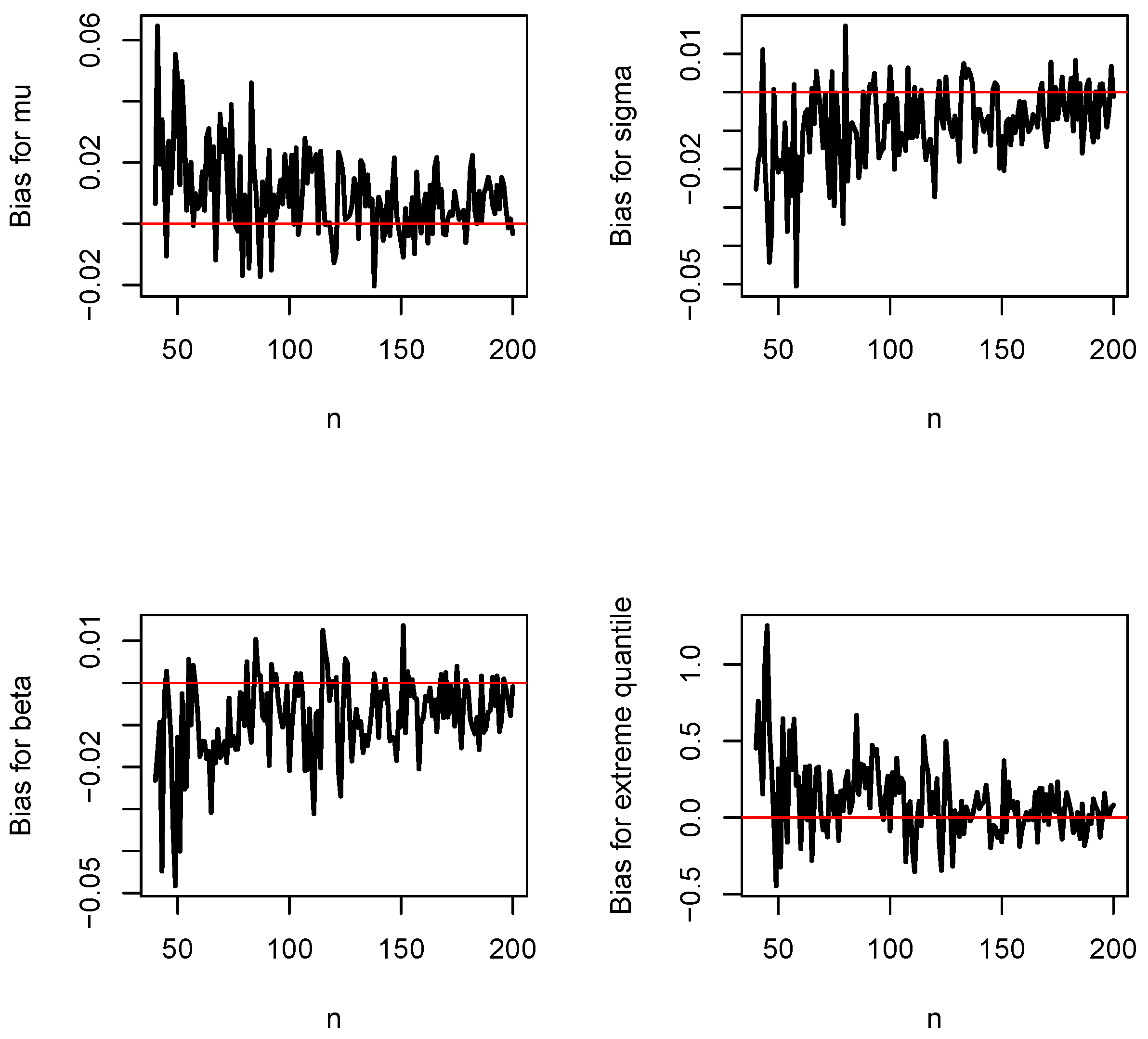
Figure A2.
Mean squared errors of , , and versus n when and .
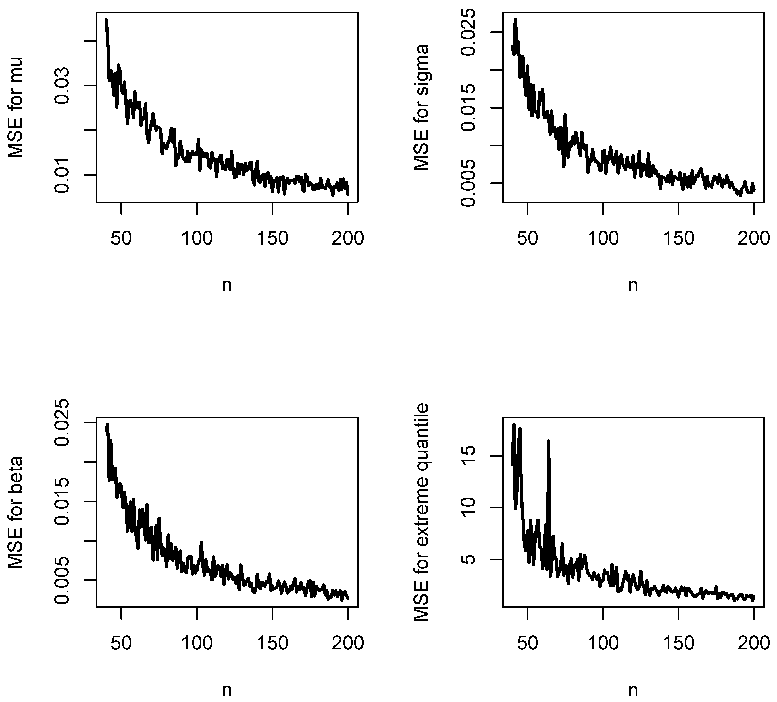
Figure A3.
Coverage lengths for , , and versus n when and .
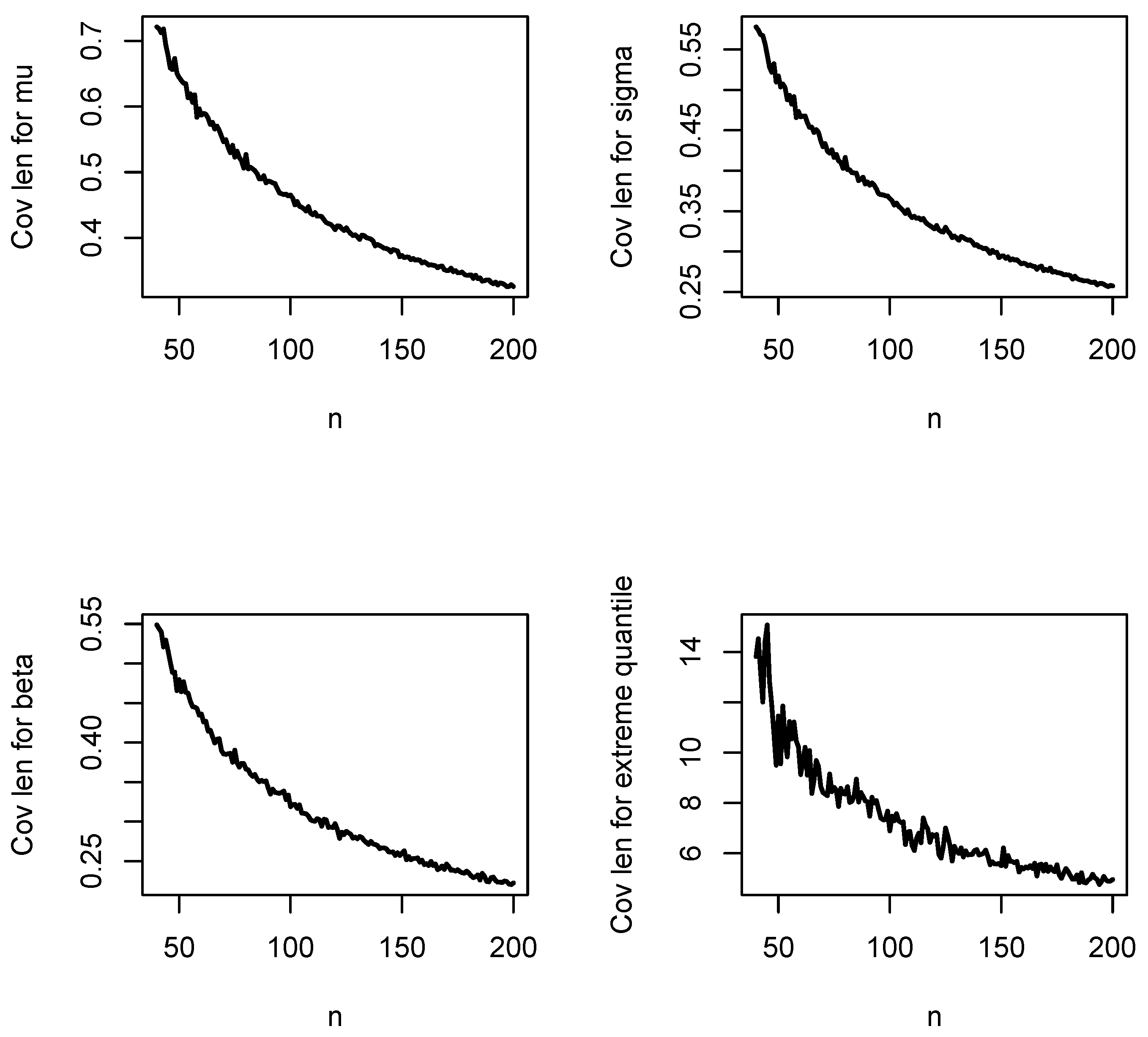
Figure A4.
Coverage probabilities for , , and versus n when and .
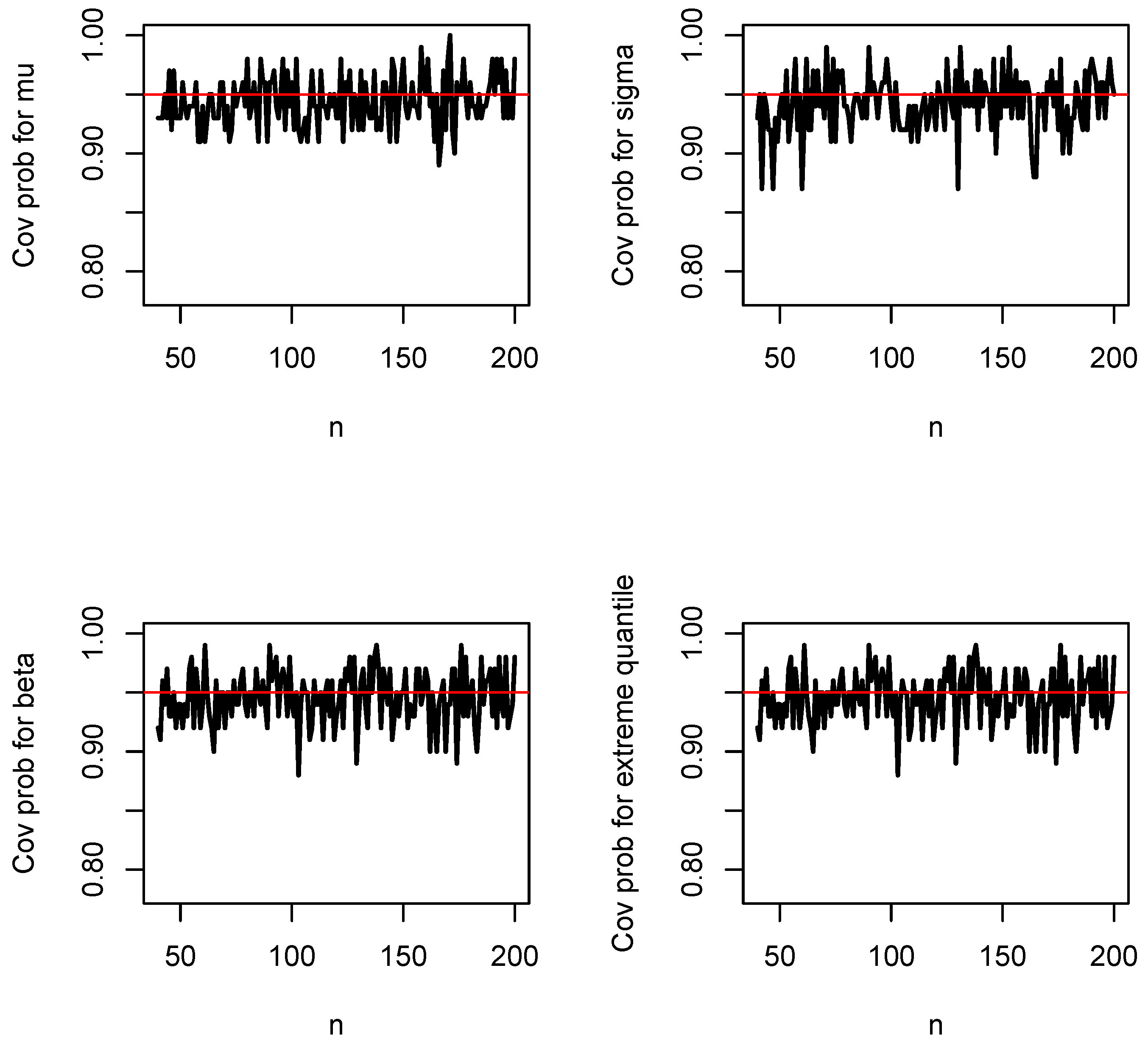
Figure A5.
Biases of , , and versus n when and .
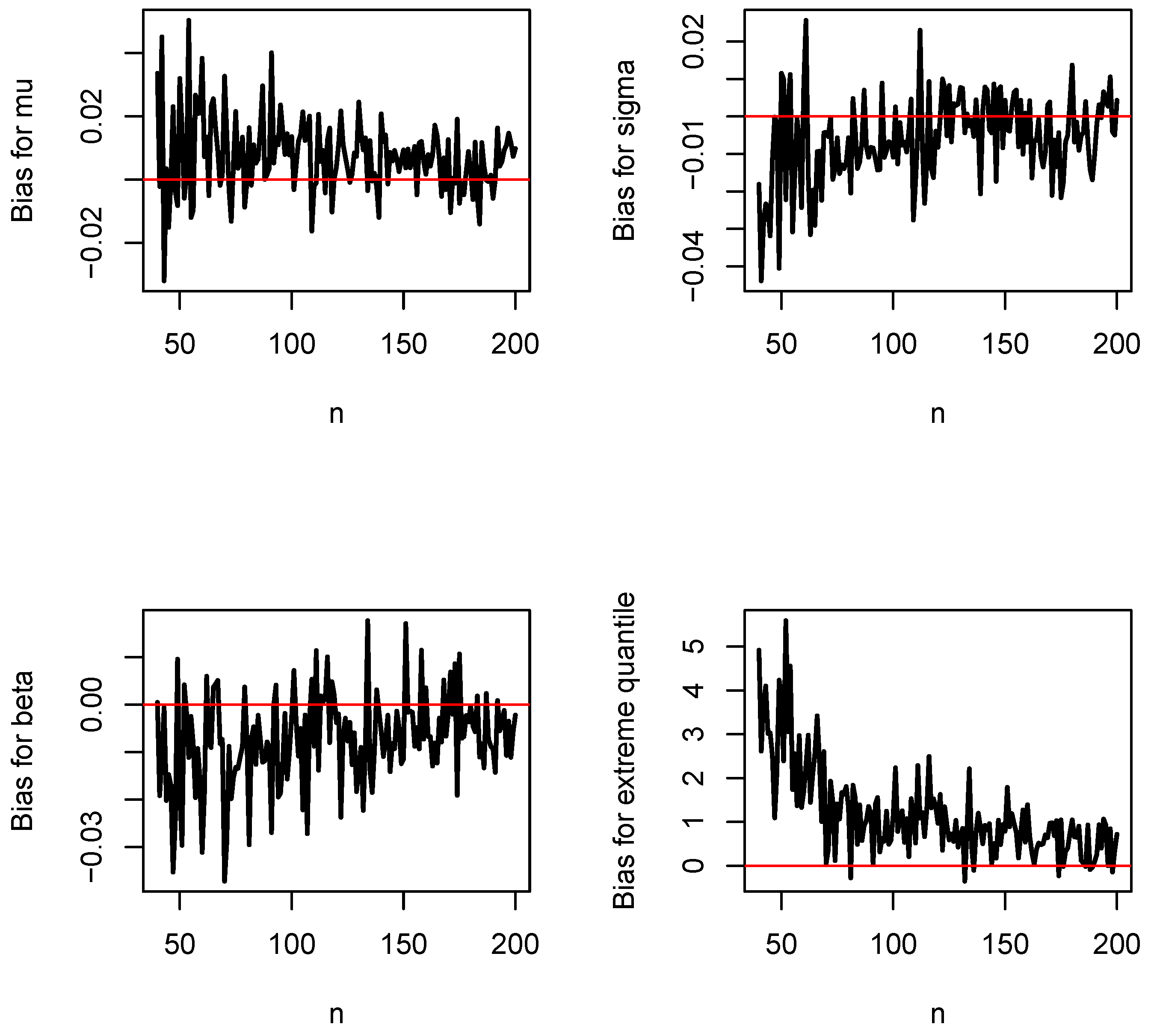
Figure A6.
Mean squared errors of , , and versus n when and .
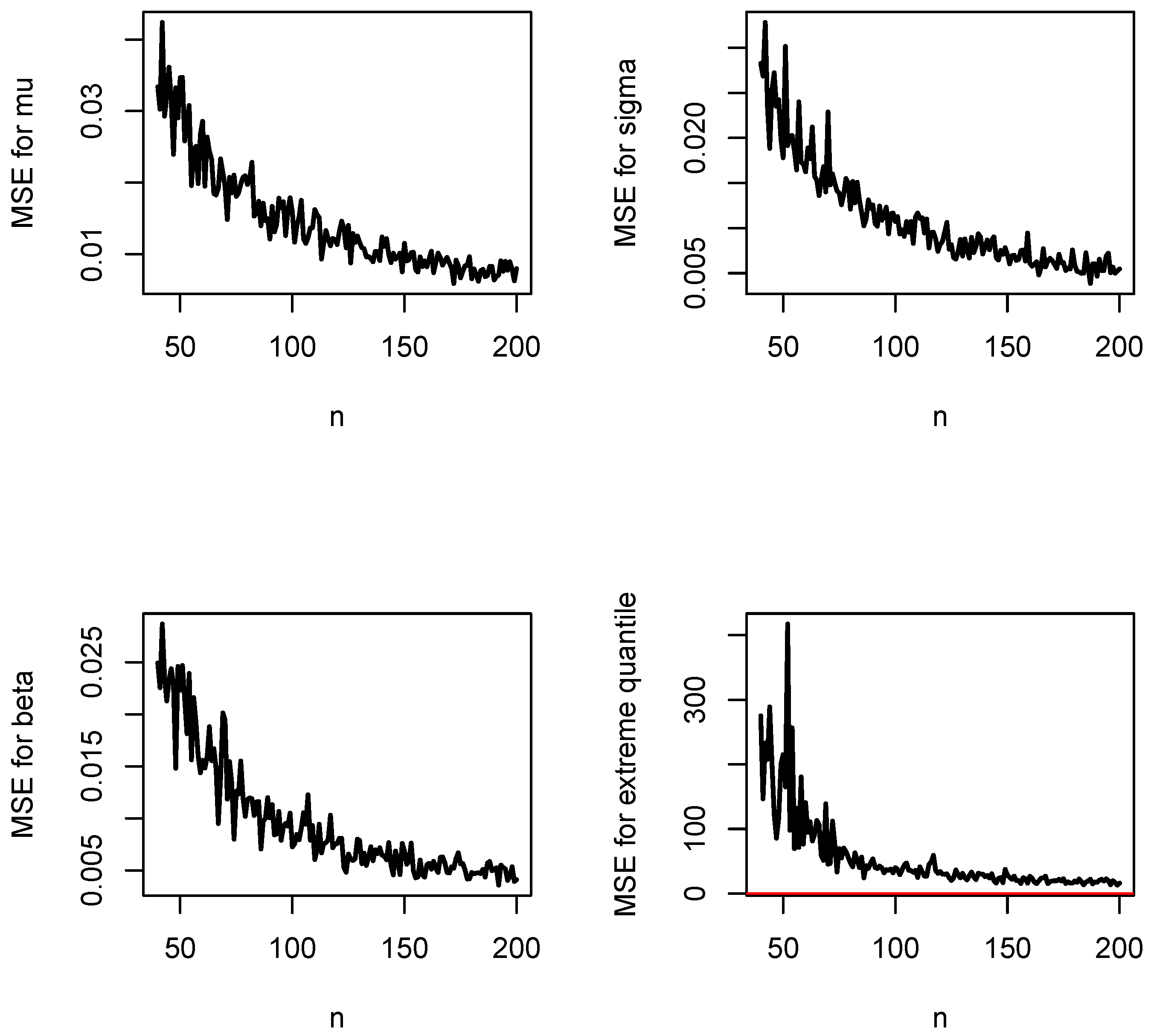
Figure A7.
Coverage lengths for , , and versus n when and .
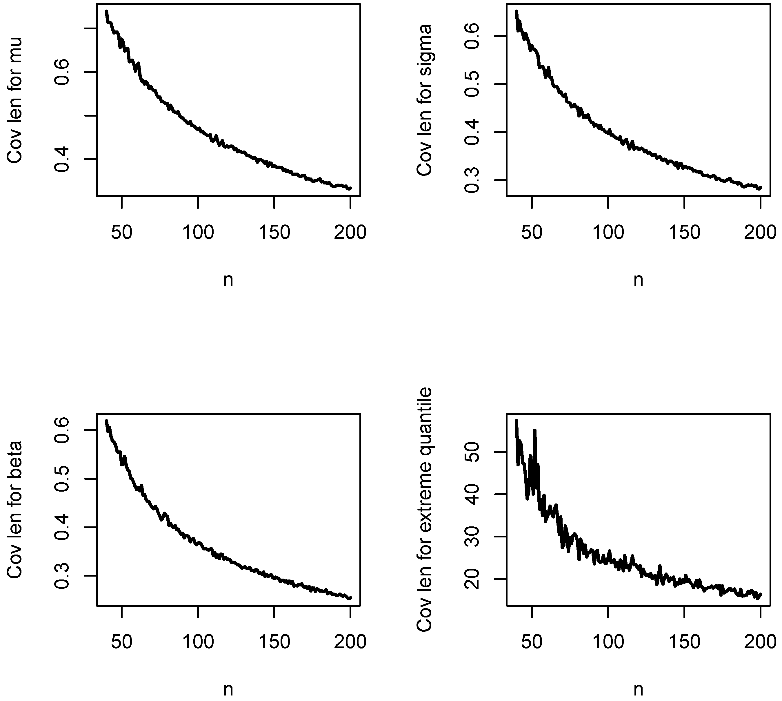
Figure A8.
Coverage probabilities for , , and versus n when and .
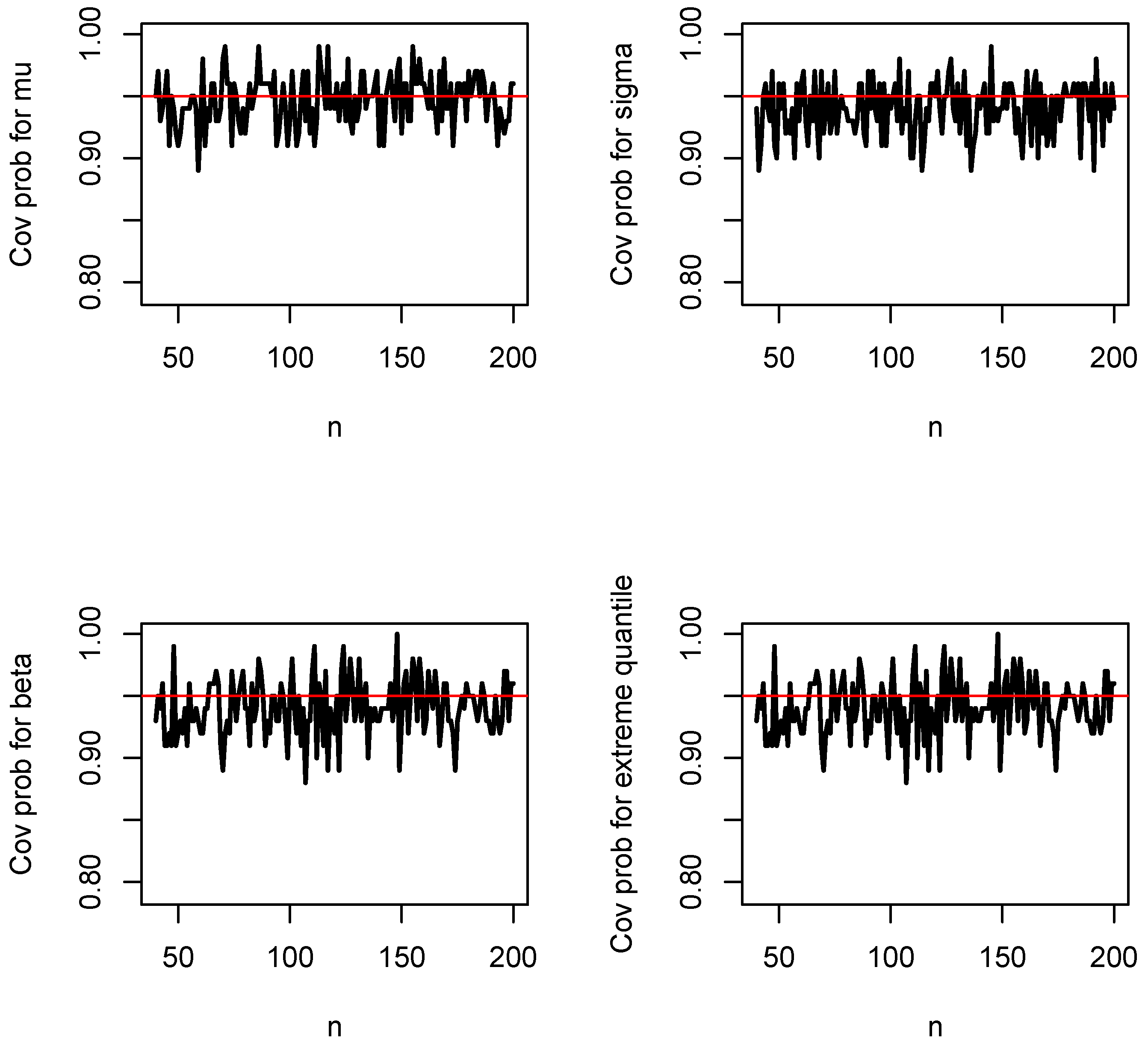
Figure A9.
Biases of , , and versus n when and .
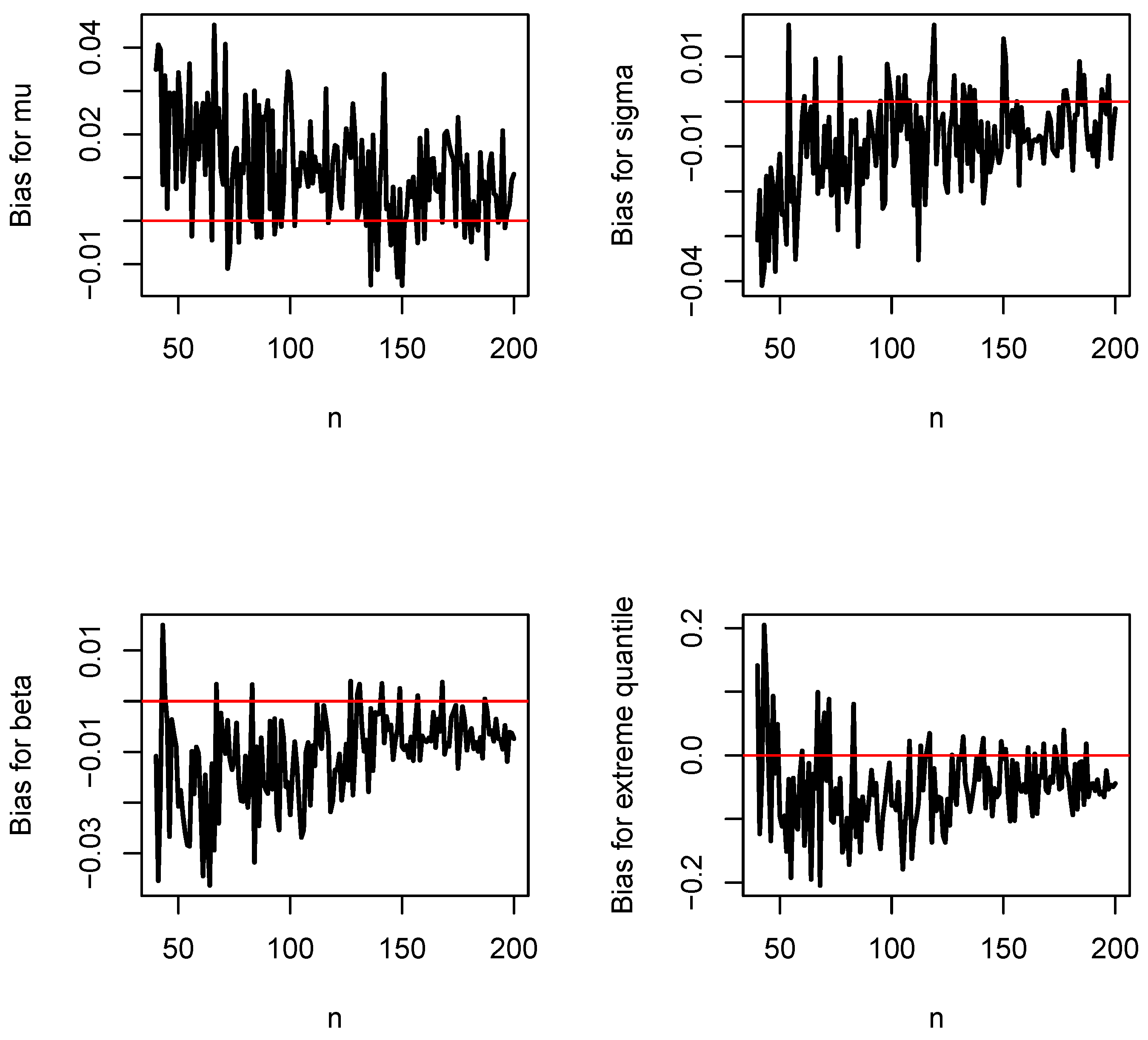
Figure A10.
Mean squared errors of , , and versus n when and .
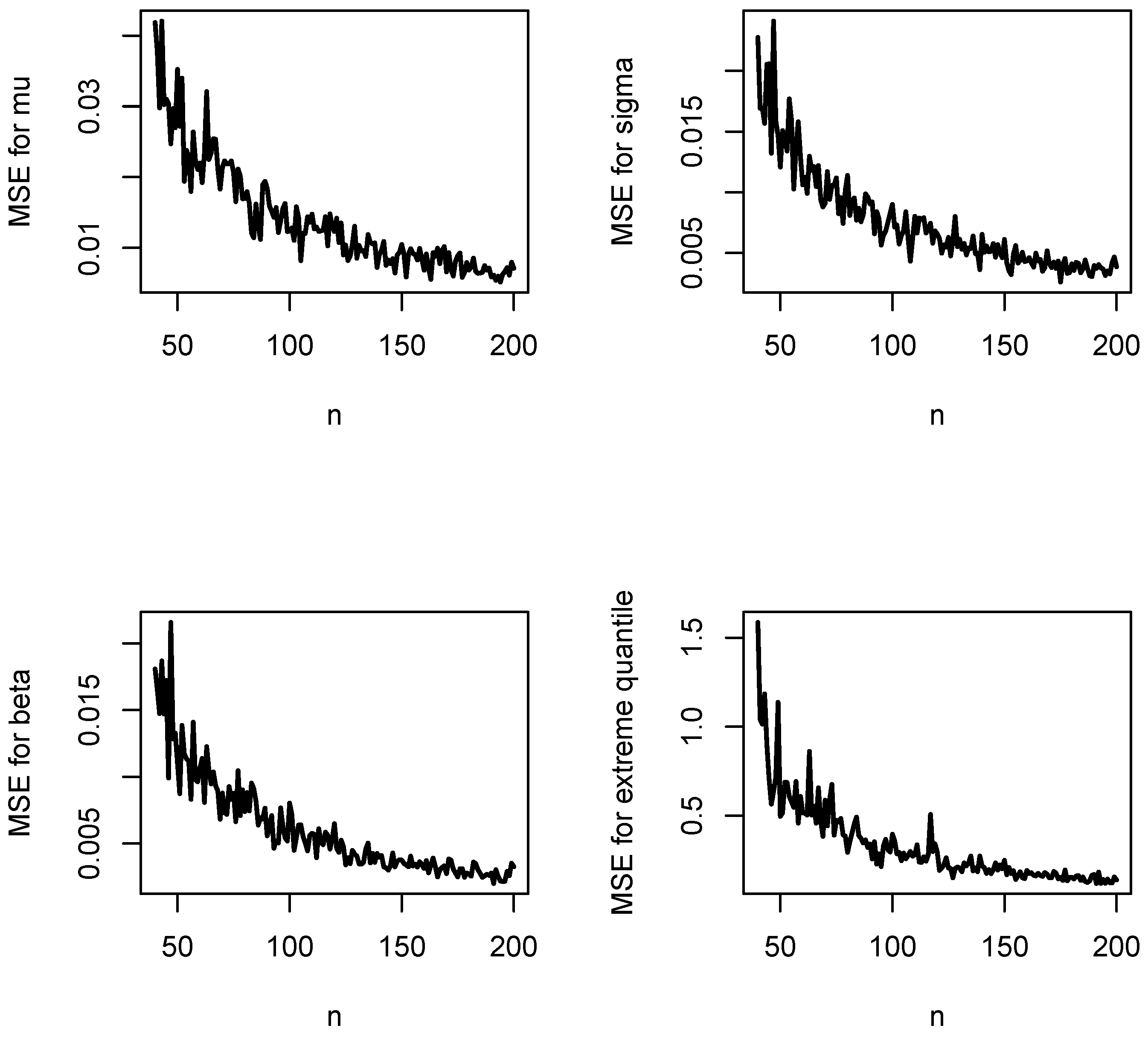
Figure A11.
Coverage lengths for , , and versus n when and .
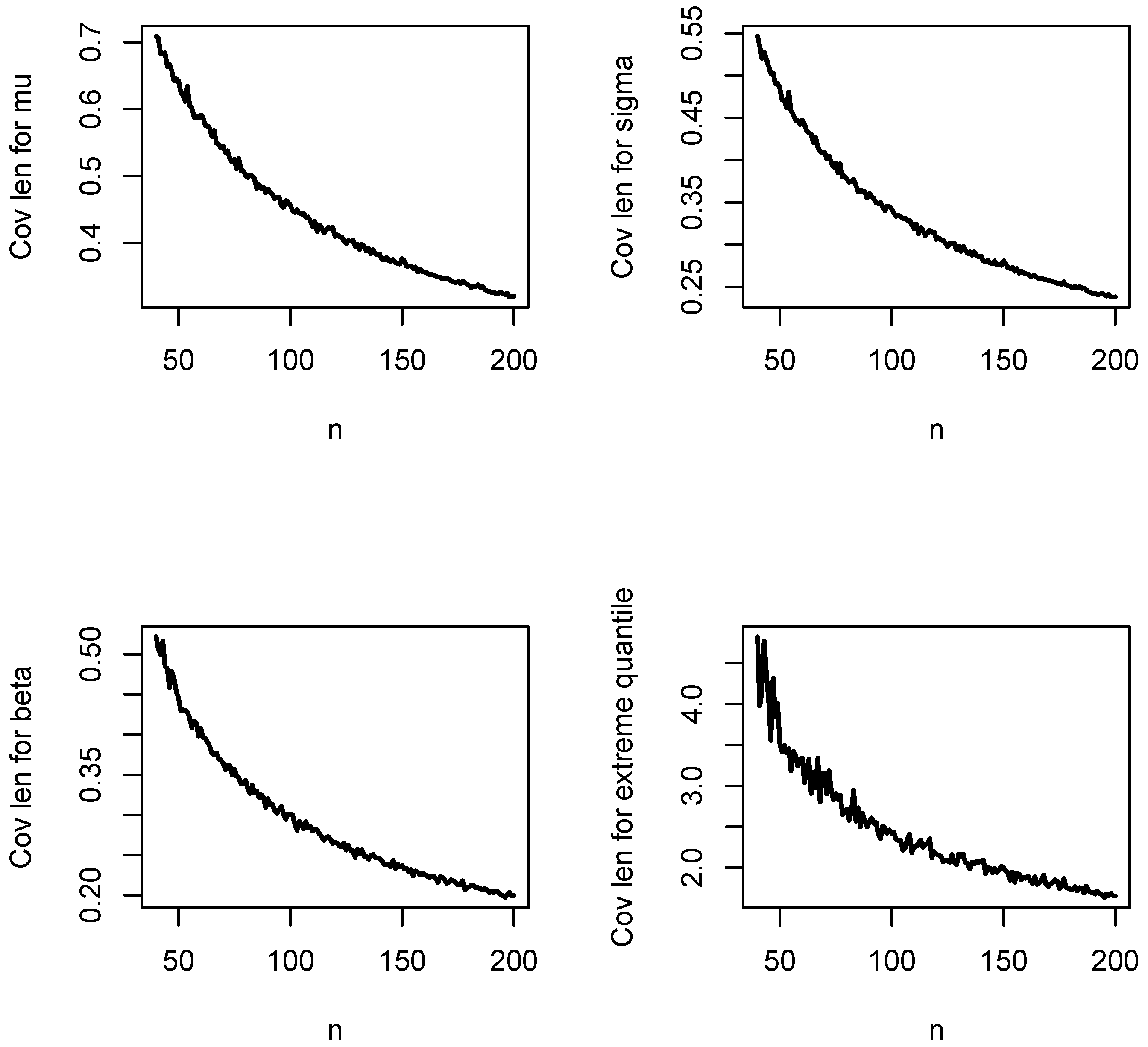
Figure A12.
Coverage probabilities for , , and versus n when and .
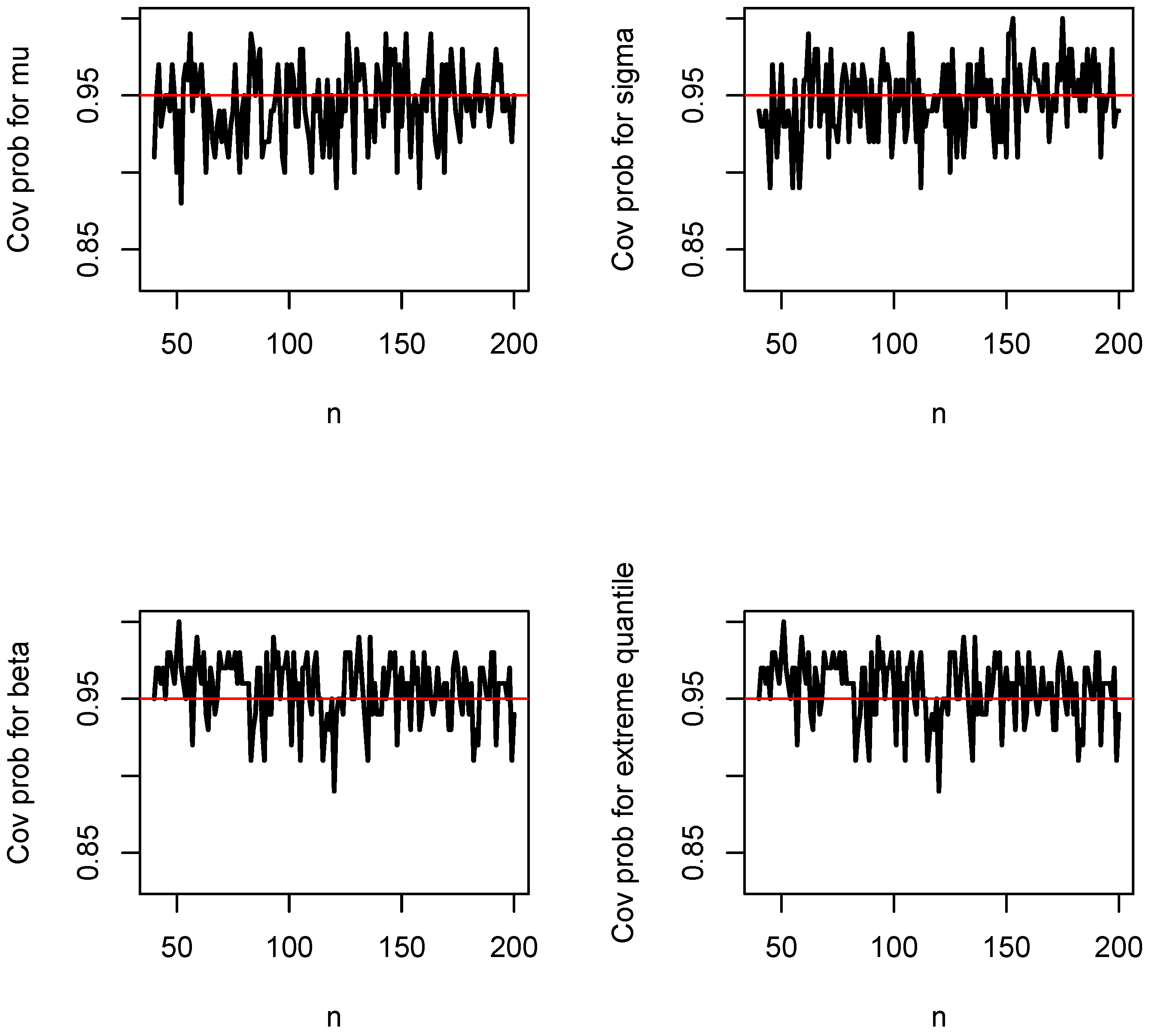
Figure A13.
Biases of , , and versus n when and .
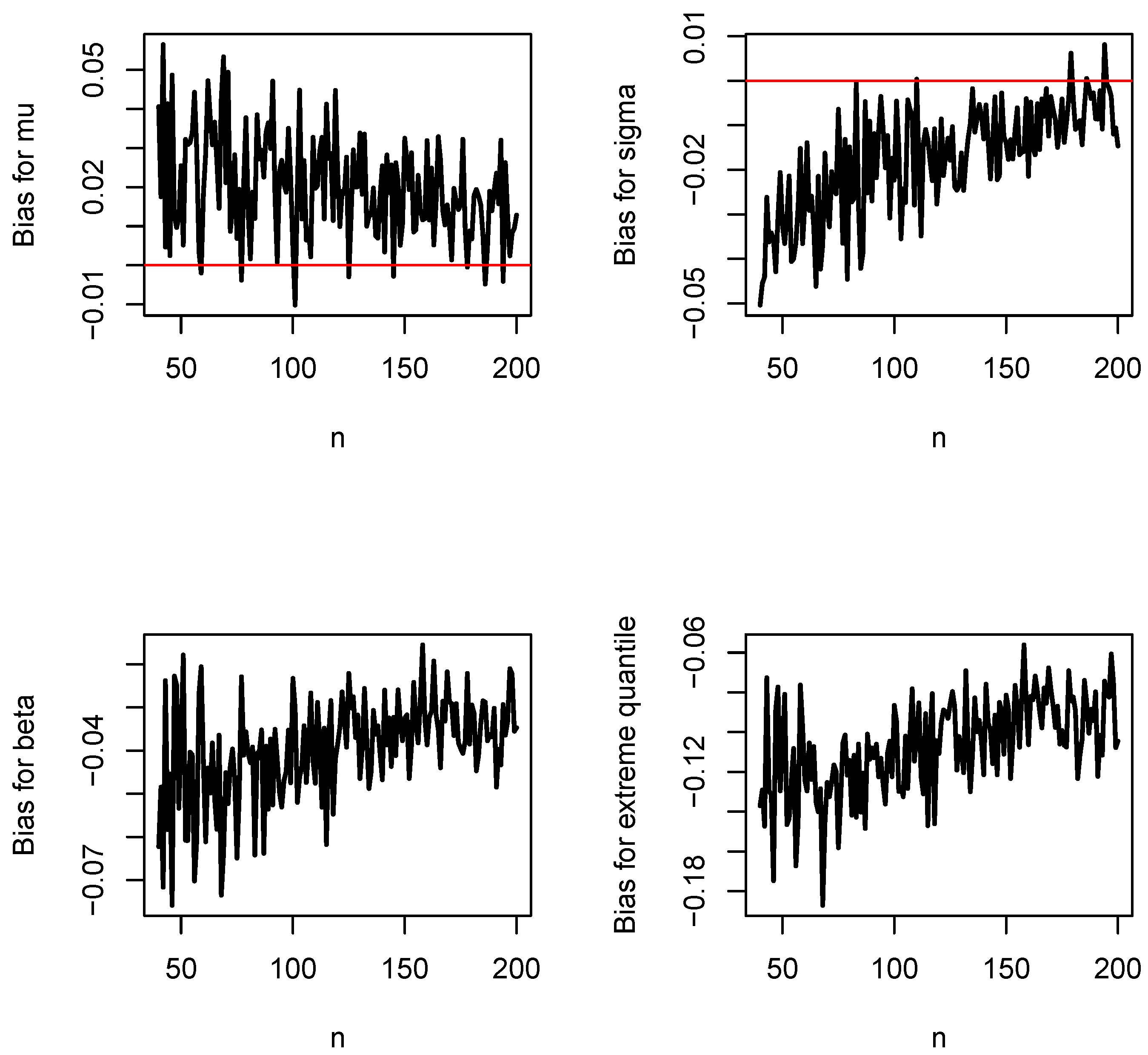
Figure A14.
Mean squared errors of , , and versus n when and .
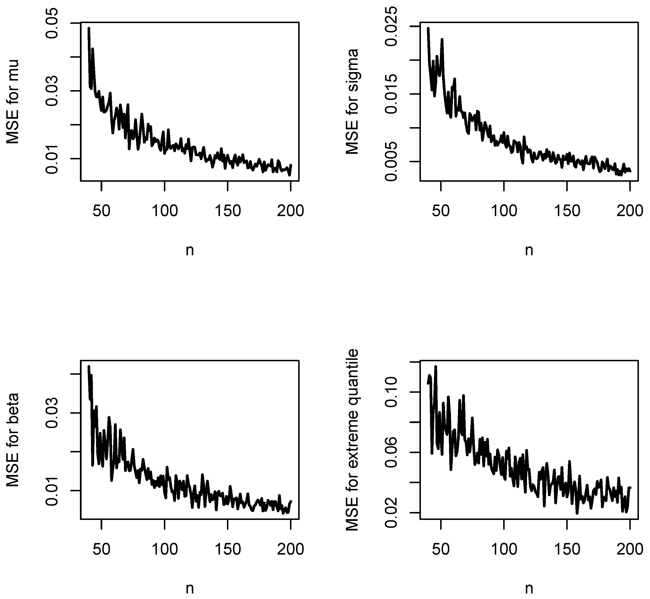
Figure A15.
Coverage lengths for , , and versus n when and .
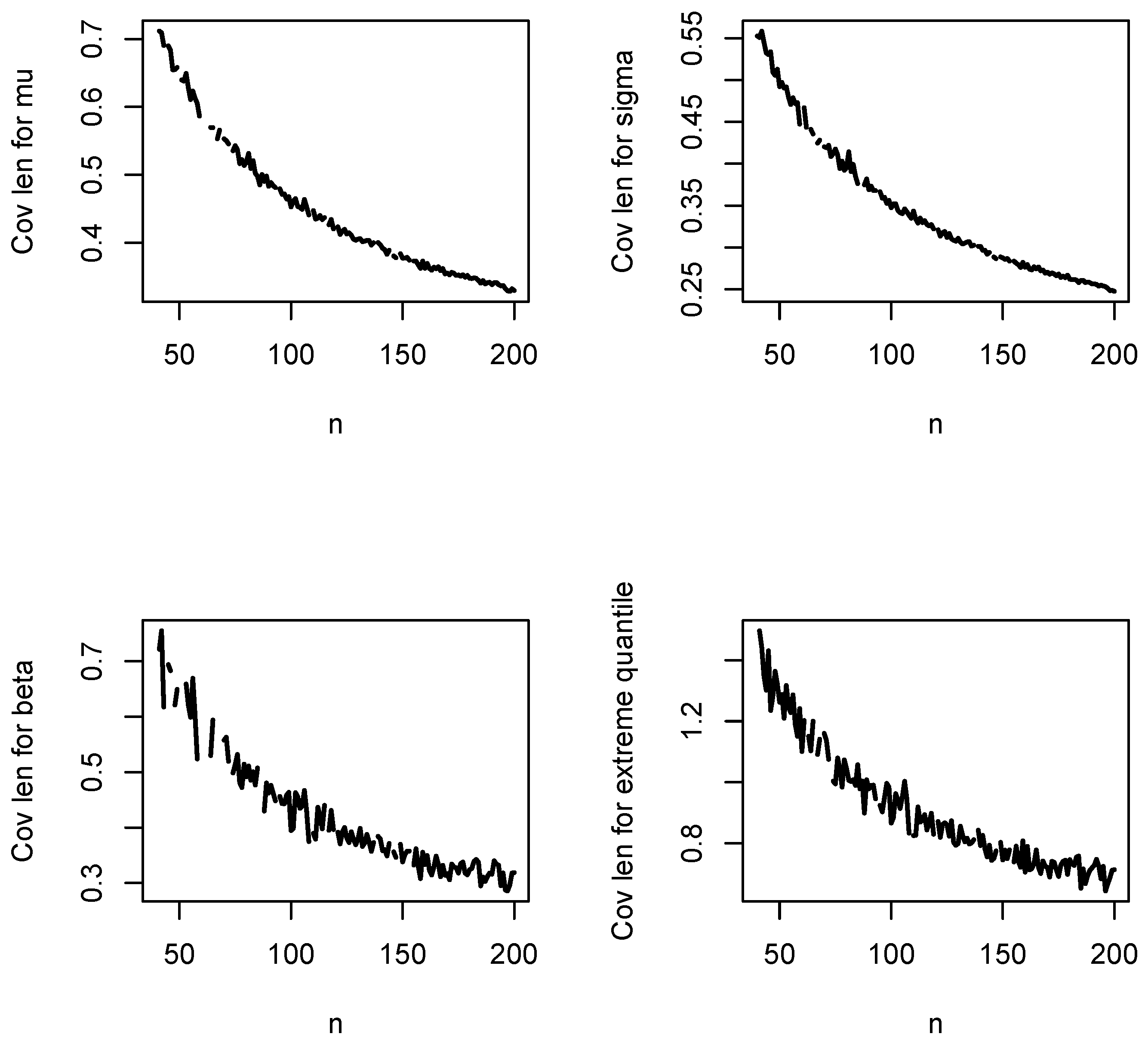
Figure A16.
Coverage probabilities for , , and versus n when and .
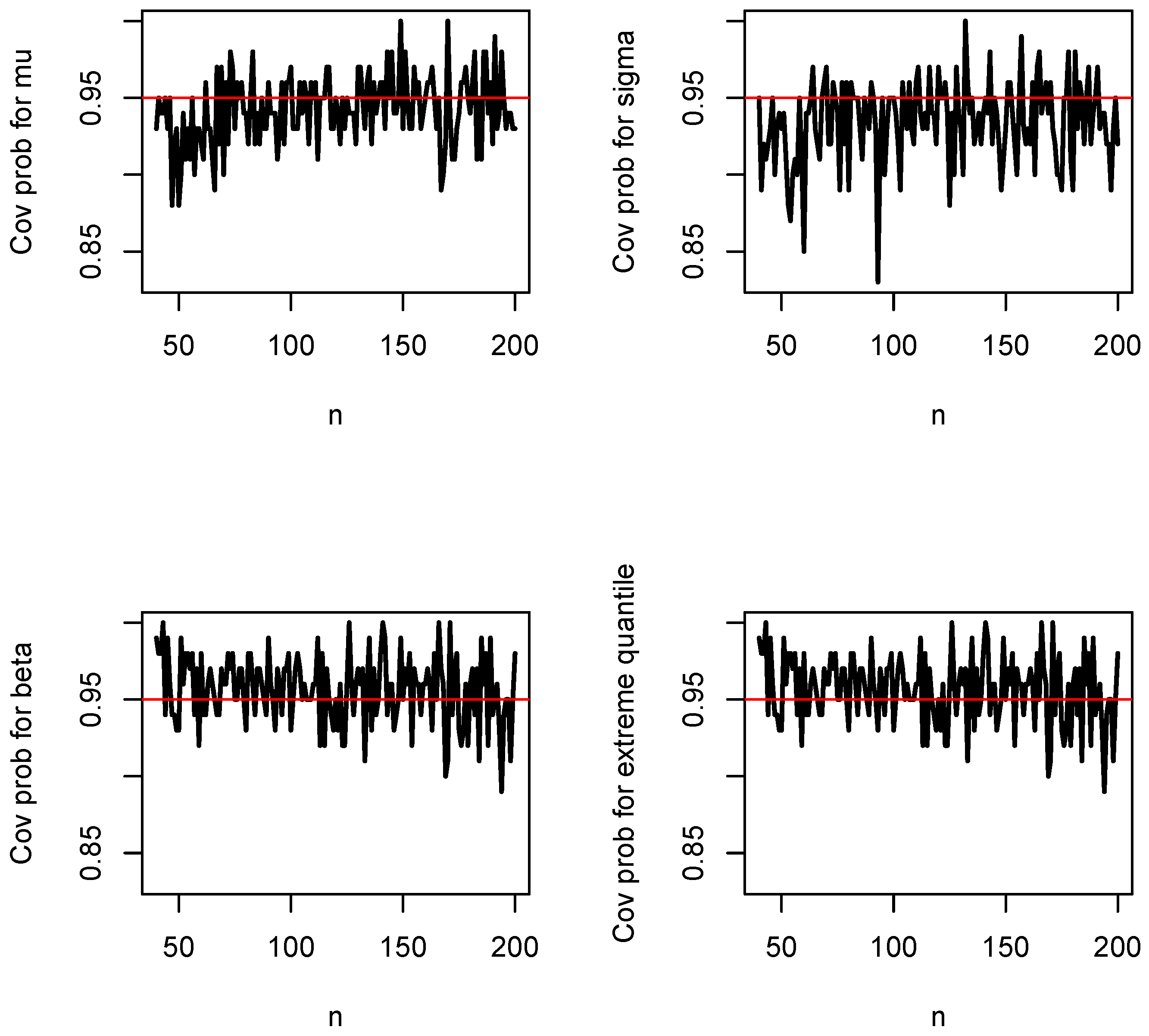
Figure A17.
Biases of , , and versus n when and .
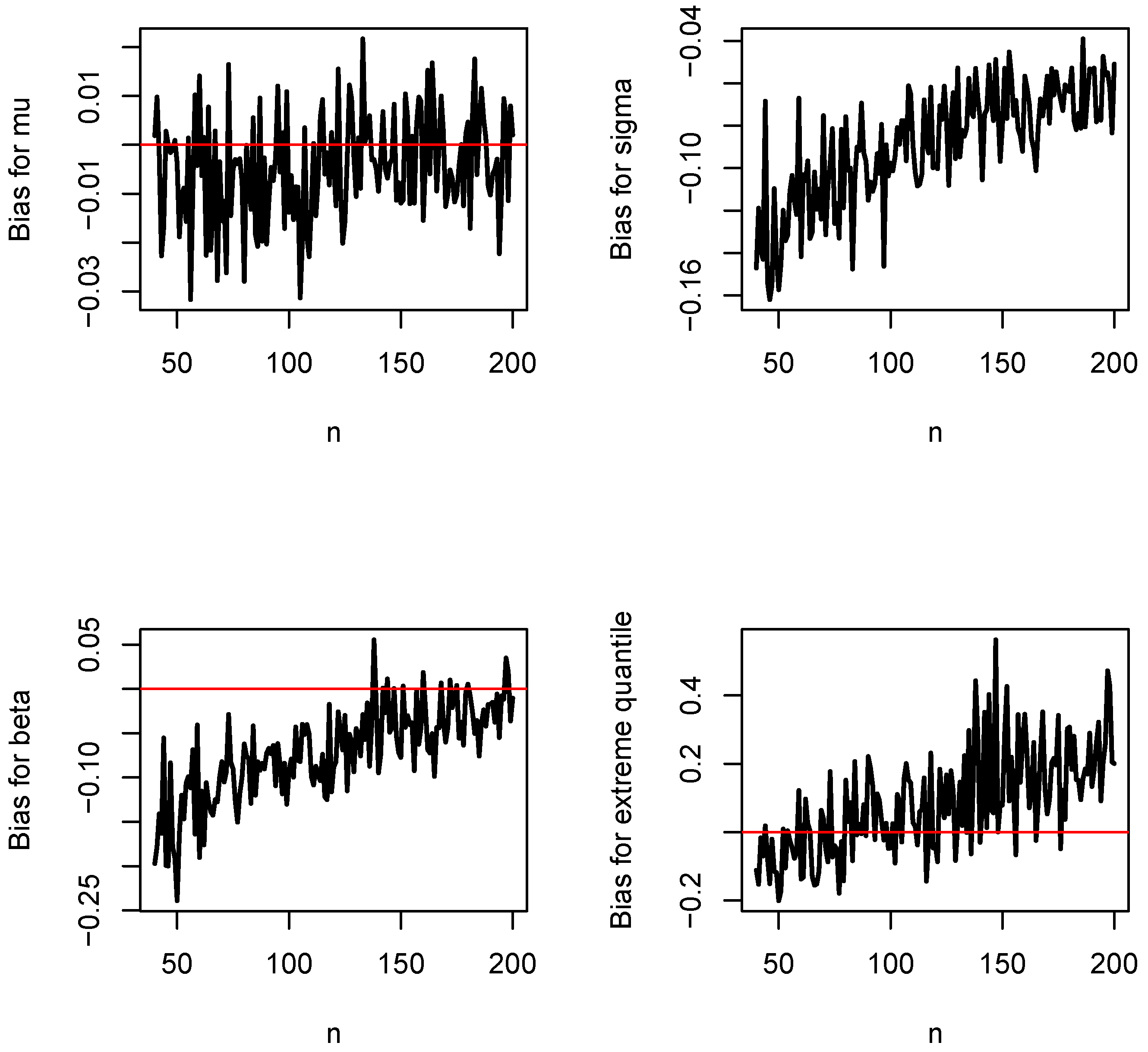
Figure A18.
Mean squared errors of , , and versus n when and .
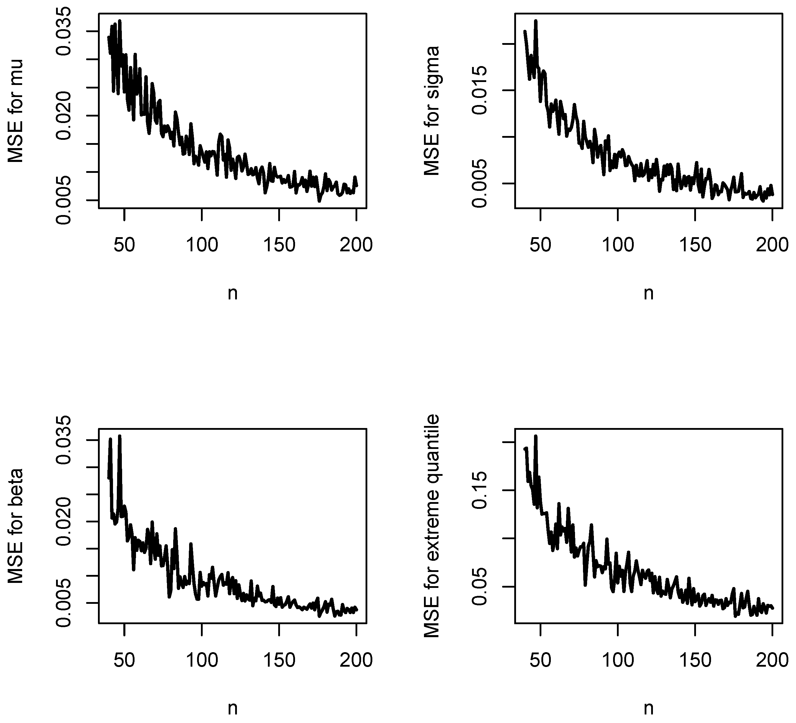
Figure A19.
Coverage lengths for , , and versus n when and .
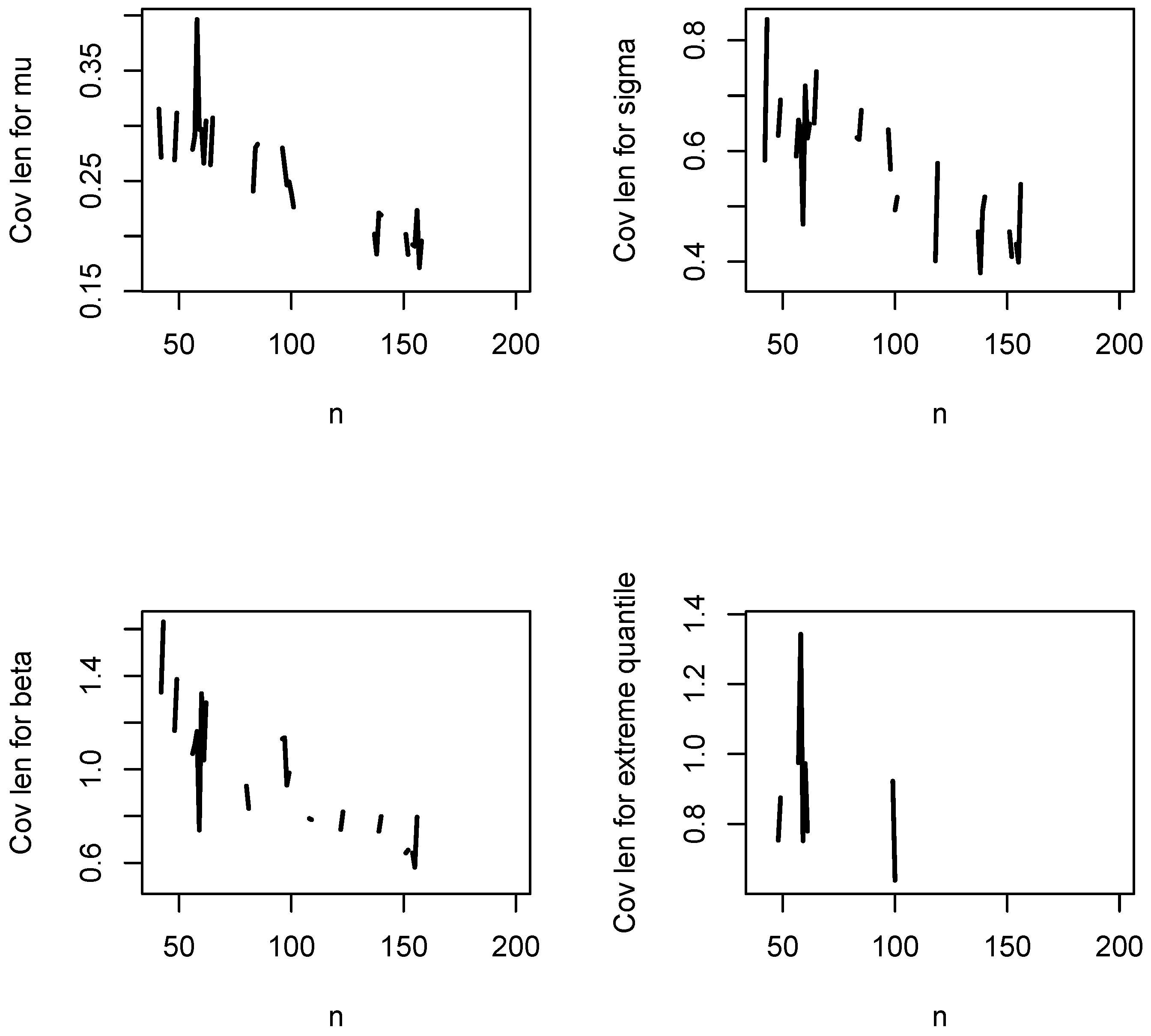
Figure A20.
Coverage probabilities for , , and versus n when and .
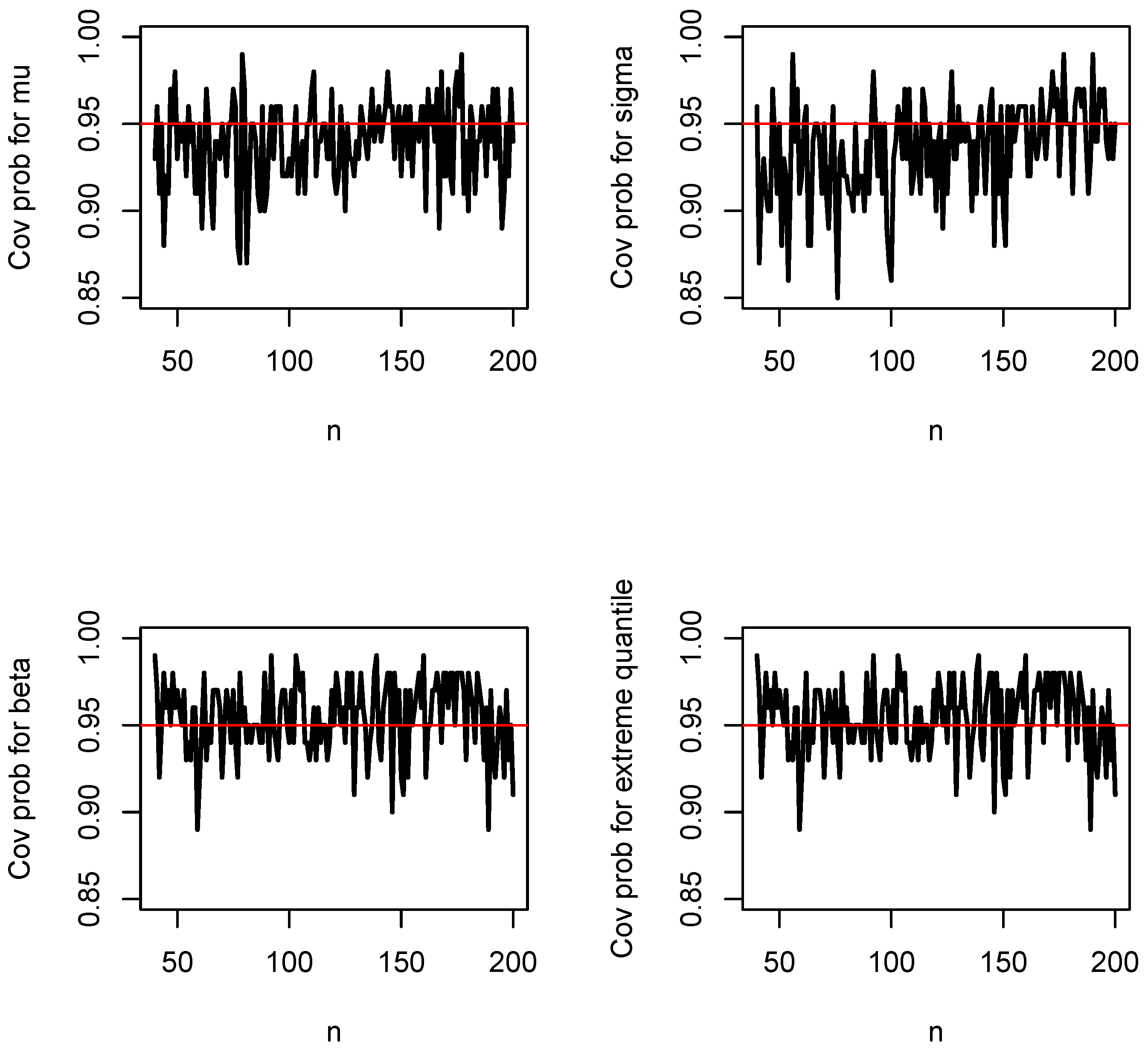
References
- Fisher, R.A.; Tippett, L.H.C. Limiting forms of the frequency distribution of the largest and smallest member of a sample. Proc. Camb. Philos. Soc. 1928, 24, 180–190. [Google Scholar] [CrossRef] [Scilit]
- Gnedenko, B.V. Sur la distribution limite du terme maximum d’une série aléatoire. Ann. Math. 1943, 44, 423–453. [Google Scholar] [CrossRef] [Scilit]
- Jenkinson, A.F. The frequency distribution of the annual maximum (or minimum) values of meteorological elements. Q. J. R. Meteorol. Soc. 1955, 81, 158–171. [Google Scholar] [CrossRef] [Scilit]
- Cherif, S. A generalized extreme value approach for the analysis of stationary climatic covariate in a Mediterranean city. Atmos. Sci. Lett. 2025, 26, e1291. [Google Scholar] [CrossRef] [Scilit]
- Jiao, Z.; Yuan, J.; Farnham, C.; Emura, K. Assessing the risk of extreme precipitation in Japan through GEV distribution and spatial modeling. J. Hydrol. Reg. Stud. 2026, 63, 103107. [Google Scholar] [CrossRef] [Scilit]
- Hossain, I.; Gato-Trinidad, S.; Imteaz, M.A. Seasonal and spatial variations in General Extreme Value (GEV) distribution shape parameter for estimating extreme design rainfall in Tasmania. Water 2026, 18, 319. [Google Scholar] [CrossRef] [Scilit]
- Zhang, C.; Fu, X.; Yang, D.; Zhang, P.; Zhang, Y. GEV distribution-enhanced Fourier diffusion model for extreme value capture in day-ahead photovoltaic scenario generation. Appl. Energy 2026, 409, 127472. [Google Scholar] [CrossRef] [Scilit]
- Zhang, F.; Zheng, S.; Ma, F.; Yin, Q.; Zhou, Y. SAR image change detection via generalized extreme value (GEV) modeling. Pattern Recognit. 2026, 170, 112040. [Google Scholar] [CrossRef] [Scilit]
- Hosking, J.R.M.; Wallis, J.R.; Wood, E.F. Estimation of the generalized extreme-value distribution by the method of probability-weighted moments. Technometrics 1985, 27, 251–261. [Google Scholar] [CrossRef]
- Leadbetter, M.R.; Lindgren, G.; Rootzén, H. Extremes and Related Properties of Random Sequences and Processes; Springer: New York, NY, USA, 1983. [Google Scholar]
- Galambos, J. The Asymptotic Theory of Extreme Order Statistics; Robert E. Krieger Publishing Company: Malabar, FL, USA, 1987. [Google Scholar]
- Resnick, S.I. Extreme Values, Regular Variation and Point Processes; Springer: New York, NY, USA, 1987. [Google Scholar]
- Embrechts, P.; Klüppelberg, C.; Mikosch, T. Modelling Extremal Events for Insurance and Finance; Springer: Berlin/Heidelberg, Germany, 1997. [Google Scholar]
- Kotz, S.; Nadarajah, S. Extreme Value Distributions: Theory and Applications; Imperial College Press: London, UK, 2000. [Google Scholar]
- Coles, S.G. An Introduction to Statistical Modeling of Extreme Values; Springer: London, UK, 2001. [Google Scholar]
- Beirlant, J.; Goegebeur, Y.; Segers, J.; Teugels, J. Statistics of Extremes: Theory and Applications; John Wiley and Sons: Chichester, UK, 2004. [Google Scholar]
- Gumbel, E.J. Statistics of Extremes; Dover Publications: Mineola, NY, USA, 2004. [Google Scholar]
- Castillo, E.; Hadi, A.S.; Balakrishnan, N.; Sarabia, J.M. Extreme Value and Related Models with Applications in Engineering and Science; John Wiley and Sons: Hoboken, NJ, USA, 2005. [Google Scholar]
- Malevergne, Y.; Sornette, D. Extreme Financial Risks: From Dependence to Risk Management; Springer: Berlin/Heidelberg, Germany, 2006. [Google Scholar]
- de Haan, L.; Ferreira, A. Extreme Value Theory: An Introduction; Springer: New York, NY, USA, 2006. [Google Scholar]
- Reiss, R.-D.; Thomas, M. Statistical Analysis of Extreme Values with Applications to Insurance, Finance, Hydrology and Other Fields; Birkhäuser Verlag: Basel, Switzerland, 2007. [Google Scholar]
- Falk, M.; Hüsler, J.; Reiss, R.-D. Laws of Small Numbers: Extremes and Rare Events; Birkhäuser/Springer Basel AG: Basel, Switzerland, 2011. [Google Scholar]
- Novak, S.Y. Extreme Value Methods with Applications to Finance; CRC Press: Boca Raton, FL, USA, 2012. [Google Scholar]
- Ahsanullah, M. Extreme Value Distributions; Atlantis Press: Paris, France, 2016. [Google Scholar]
- Nakagawa, T.; Osaki, S. The discrete Weibull distribution. IEEE Trans. Reliab. 1975, 24, 300–301. [Google Scholar] [CrossRef] [Scilit]
- Chakraborty, S.; Chakravarty, D.; Mazucheli, J.; Bertoli, W. A discrete analog of Gumbel distribution: Properties, parameter estimation and applications. J. Appl. Stat. 2021, 48, 712–737. [Google Scholar] [CrossRef] [Scilit] [PubMed]
- Hadi, N.S.; Khudhair, J.K. On discrete Fréchet distribution: Estimation and application. J. Adm. Econ. 2024, 49, 189–199. [Google Scholar] [CrossRef] [Scilit]
- Das, D.; Das, B. Discretized Fréchet–Weibull distribution: Properties and application. J. Indian Soc. Probab. Stat. 2023, 24, 243–282. [Google Scholar] [CrossRef] [Scilit]
- Akkanphudit, T. The discrete Gompertz–Weibull–Fréchet distribution: Properties and applications. Lobachevskii J. Math. 2023, 44, 3663–3672. [Google Scholar] [CrossRef] [Scilit]
- Das, D.; Alshammari, T.S.; Rashedi, K.A.; Das, B.; Hazarika, P.J.; Eliwa, M.S. Discrete joint random variables in Fréchet–Weibull distribution: A comprehensive mathematical framework with simulations, goodness-of-fit analysis, and informed decision-making. Mathematics 2024, 12, 3401. [Google Scholar] [CrossRef] [Scilit]
- Hitz, A.S.; Davis, R.A.; Samorodnitsky, G. Discrete extremes. J. Data Sci. 2024, 22, 524–536. [Google Scholar] [CrossRef] [Scilit]
- Dkengne Sielenou, P.A.; Eckert, N.; Naveau, P. Extreme value theory for integer-valued random variables. In Proceedings of the Conference on Extreme Value Modeling and Water Resources, Lyon, France, 13–24 June 2016. [Google Scholar] [CrossRef]
- Tiago de Oliveira, J. Statistical Analysis of Extremes; Pendor: Lisbon, Portugal, 1997. [Google Scholar]
- Tabony, R.C. Extreme value analysis in meteorology. Meteorol. Mag. 1983, 112, 77–98. [Google Scholar]
- Chandler, R.E.; Bate, S. Inference for clustered data using the independence loglikelihood. Biometrika 2007, 94, 167–183. [Google Scholar] [CrossRef] [Scilit]
- Stephenson, A.G. evd: Extreme value distributions. R News 2002, 2, 31–32. [Google Scholar]
- R Core Team. R: A Language and Environment for Statistical Computing; R Foundation for Statistical Computing: Vienna, Austria, 2025. [Google Scholar]
- Smith, R.L. Maximum likelihood estimation in a class of non-regular cases. Biometrika 1985, 72, 67–90. [Google Scholar] [CrossRef]
- Davison, A.C.; Smith, R.L. Models for exceedances over high thresholds. J. R. Stat. Soc. Ser. B 1990, 52, 393–442. [Google Scholar] [CrossRef] [Scilit]
- van der Vaart, A.W. Asymptotic Statistics; Cambridge University Press: Cambridge, UK, 1998. [Google Scholar]
- Cox, D.R.; Hinkley, D.V. Theoretical Statistics; Chapman and Hall: London, UK, 1974. [Google Scholar]
- Kreutz, C. An easy and efficient approach for testing identifiability. Bioinformatics 2018, 34, 1913–1921. [Google Scholar] [CrossRef] [Scilit] [PubMed]
- Kolmogorov, A. Sulla determinazione empirica di una legge di distribuzione. G. Dell’istituto Ital. Degli Attuari 1933, 4, 83–91. [Google Scholar]
- Smirnov, N. Table for estimating the goodness of fit of empirical distributions. Ann. Math. Stat. 1948, 19, 279–281. [Google Scholar] [CrossRef] [Scilit]
- Choulakian, V.; Lockhart, R.A.; Stephens, M.A. Cramér–von Mises statistics for discrete distributions. Can. J. Stat. 1994, 22, 125–137. [Google Scholar] [CrossRef] [Scilit]
- Shannon, C.E. A mathematical theory of communication. Bell Syst. Tech. J. 1948, 27, 379–423. [Google Scholar]
- Shannon, C.E. A mathematical theory of communication. Bell Syst. Tech. J. 1948, 27, 623–656. [Google Scholar] [CrossRef] [Scilit]
- Kullback, S.; Leibler, R.A. On information and sufficiency. Ann. Math. Stat. 1951, 22, 79–86. [Google Scholar] [CrossRef] [Scilit]
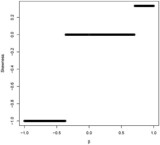
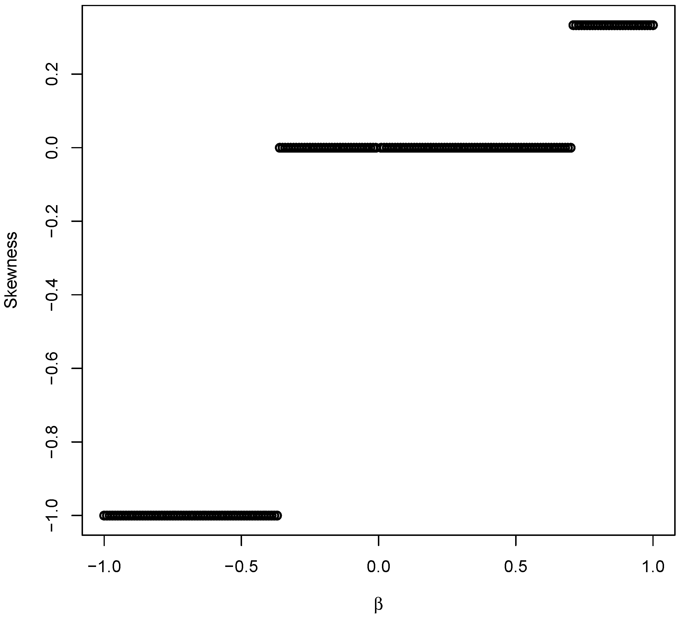
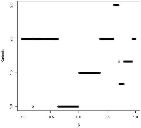
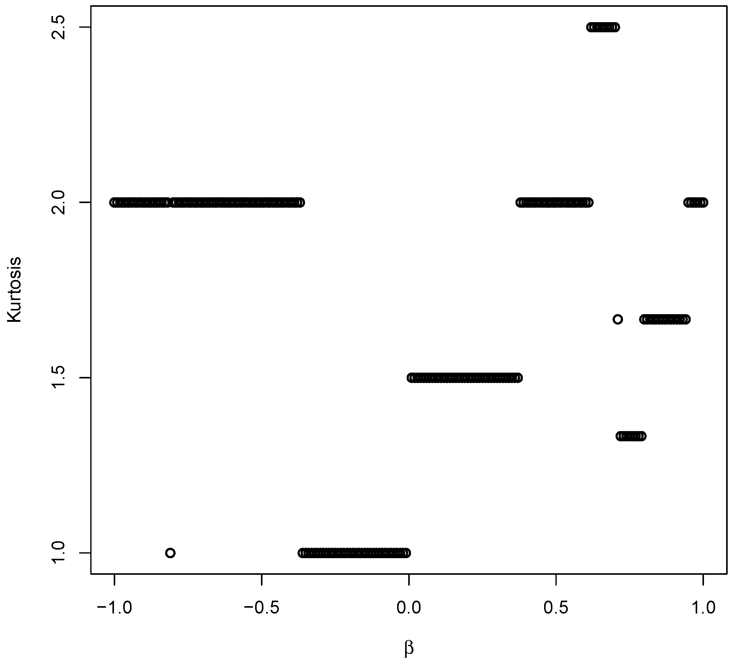
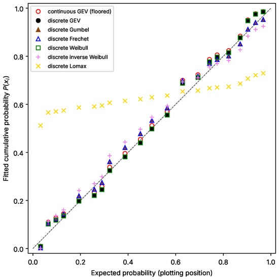
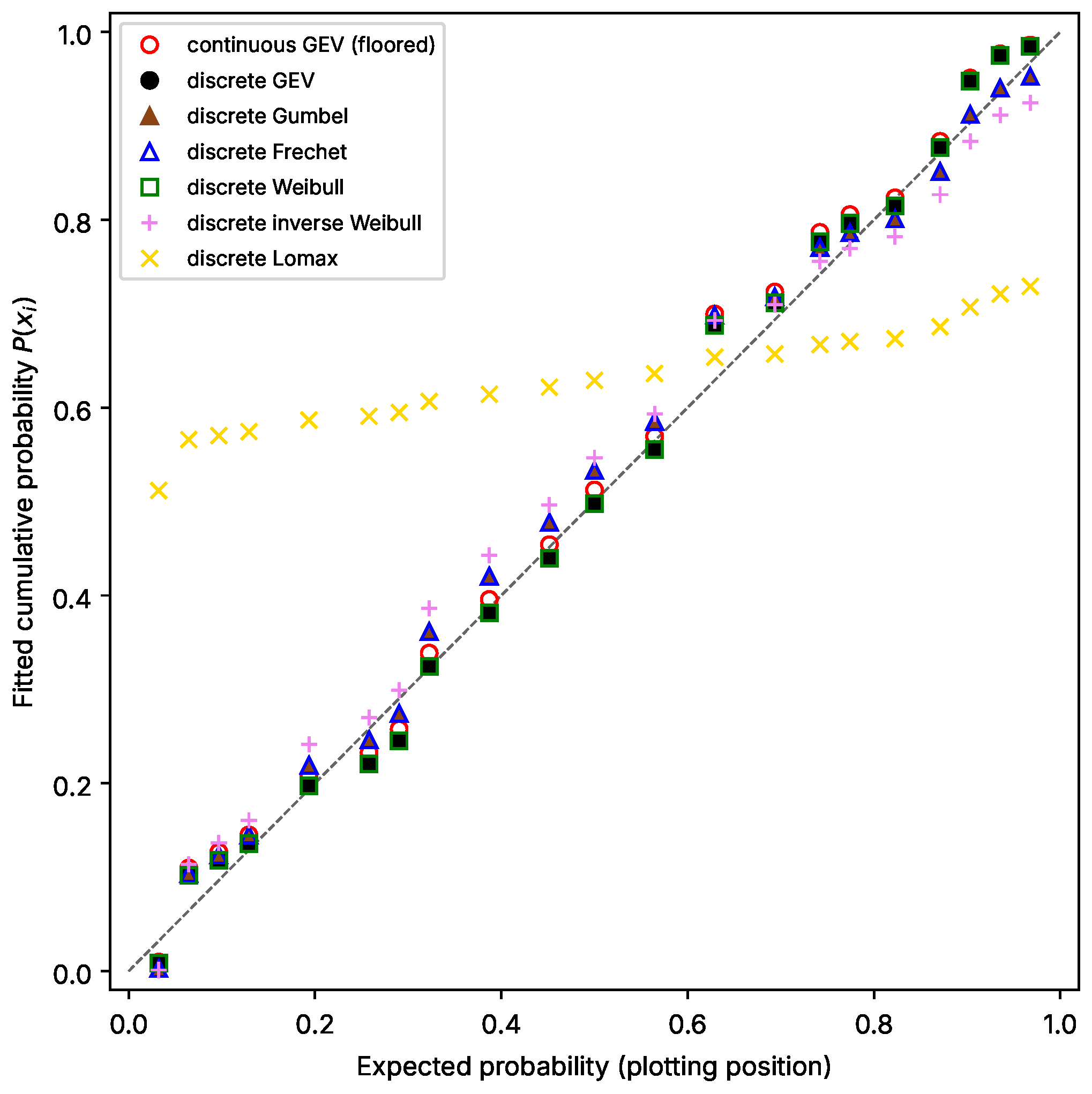
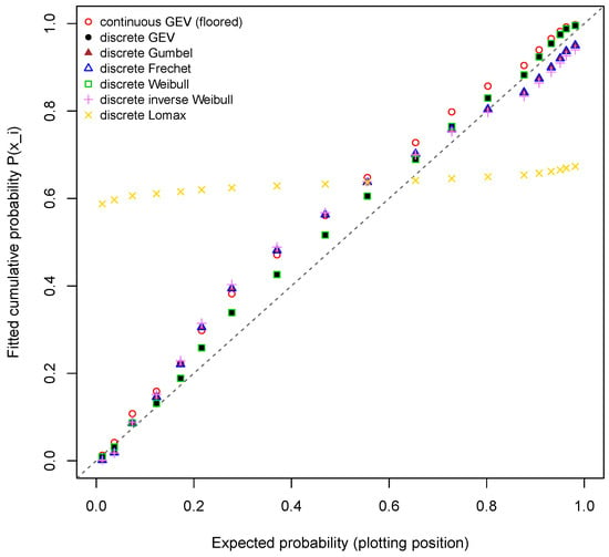
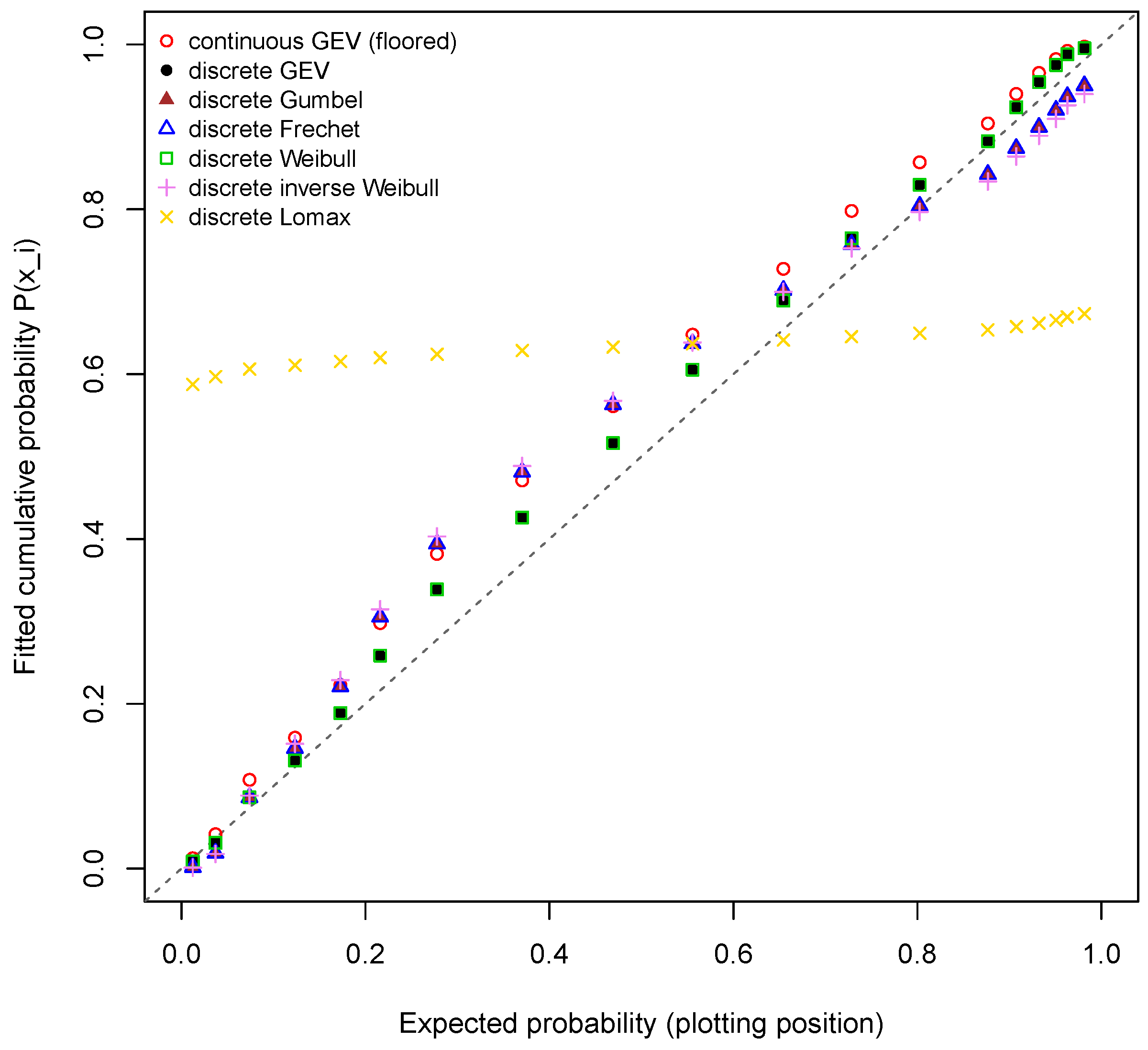

Disclaimer/Publisher’s Note: The statements, opinions and data contained in all publications are solely those of the individual author(s) and contributor(s) and not of MDPI and/or the editor(s). MDPI and/or the editor(s) disclaim responsibility for any injury to people or property resulting from any ideas, methods, instructions or products referred to in the content. |
© 2026 by the authors. Licensee MDPI, Basel, Switzerland. This article is an open access article distributed under the terms and conditions of the Creative Commons Attribution (CC BY) license.