An Efficient Automated Geometry Reasoning Method via Knowledge Merging and Semi-Conditional Rules

Abstract

This paper presents KM-SCR, a deductive-database system for automated geometry reasoning that aims to reduce redundant knowledge representation and inference overhead. First, a geometric-object merging mechanism consolidates collinear or coplanar objects and updates their associated relations, reducing redundant representations in the knowledge base. Second, a chain-of-equalities representation facilitates quantitative inference and supports algebraic reasoning through matrix-column compression and equation-system simplification. Third, semi-conditional rules divide rule-matching conditions into base conditions and remaining constraints, enabling staged candidate generation and constraint verification to reduce unnecessary matching operations. We establish the equivalence between semi-conditional rules and their original formulations at the rule-instance level and integrate the three mechanisms into an iterative reasoning workflow. Experiments on all 293 problems in FormalGeo7k-L6 show that KM-SCR solves 288 instances (98.29%), with a mean solving time of 4.06 s among successfully solved instances. On 40 sampled problems from each of levels L1–L5, the success rates range from 97.50% to 100.00%. Further analyses of theoretical inference space, actual rule instantiations, memory consumption, and solving time assess the effects of the proposed mechanisms on knowledge redundancy and inference efficiency.

1. Introduction

Geometry Automated Theorem Proving (GATP) has long been an important research topic in artificial intelligence and mathematical mechanization. Since the emergence of the field in the twentieth century, plane geometry theorem proving has served as a benchmark for evaluating machine reasoning capabilities [1]. Major approaches to GATP include algebraic, semi-algebraic, and synthetic methods. Algebraic methods, such as Wu’s method [2] and Gröbner basis methods [3], encode geometric constraints as polynomial equations and establish conclusions through algebraic computation. These methods are powerful, although their computational steps can be difficult to interpret in geometric terms. Semi-algebraic methods, such as the area method [4], the full-angle method [5], and invariant-algebra and point-geometry approaches [6,7,8], use geometric quantities to retain geometric meaning within algebraic derivations. Synthetic methods reason directly about geometric objects and their relations by applying geometric definitions, axioms, and theorems. Their explicit intermediate deductions make it easier to inspect the logical dependencies between geometric facts and understand how a conclusion is reached. This property is valuable in mathematics education, where step-by-step proofs can help students follow and understand geometric arguments. Interactive educational tools thus provide one potential application for efficient synthetic reasoning, as timely generation of understandable proofs could support explanations and feedback during geometric exploration. These considerations motivate the development of deductive systems that combine explicit geometric reasoning with efficient inference.

Among synthetic approaches, the geometry deductive database method (GDDM) [9] and subsequent systems [10] use forward reasoning to derive geometric facts by repeatedly applying inference rules until a target is established or a reasoning fixed point is reached. Their explicit deductions support readable proofs in mathematics-education systems such as Java Geometry Expert (JGEX) [11] and NetPad [12]. Automated theorem proving has also been integrated into interactive geometry environments such as GeoGebra [13], where geometric conjectures can be explored and formally verified, and GeoGebra Discovery [14], which further extends this capability for automated discovery and verification of geometric properties. Dynamic extensions of predicates and inference rules further improve the flexibility of deductive systems [15]. Alongside these developments in deductive reasoning, learning-based approaches have increasingly been explored to guide theorem selection and proof search.

In this direction, Inter-GPS [16] combines formalized geometric representations with theorem prediction to guide symbolic reasoning. E-GPS [17] further improves search efficiency through learned problem-solving and problem-generation strategies, while Pi-GPS [18] incorporates diagrammatic information to enhance geometric problem formalization. Together, these studies explore how learned models can support symbolic geometric reasoning through improved problem representations and search guidance.

A more systematic formal foundation is provided by FormalGeo [19], which establishes a unified formal language, a geometric theorem system, a formal solver, and the FormalGeo7k benchmark. The FGeo series builds on this formalized problem-solving setting to study learned guidance for symbolic proof search. For example, FGeo-TP [20] employs language models to predict theorem sequences and prune the search space, FGeo-HyperGNet [21] models structured reasoning states as a hypertree and uses a hypergraph neural network to guide theorem selection, and FGeo-ISRL [22] further integrates inverse search, deep reinforcement learning, and Monte Carlo tree search to improve proof search on complex geometry problems. More recently, FGeo-NSS [23] continues this neuro-symbolic direction by integrating learned guidance with formal geometric deduction.

With the rise of large language models (LLMs), their strong semantic understanding and generation capabilities have opened up new research directions for geometric reasoning. Early attempts to apply LLMs to mathematical proof generation revealed challenges in maintaining rigorous logical consistency and verifiability [24]. Consequently, recent research has gradually shifted toward a neuro-symbolic collaborative reasoning paradigm, in which LLMs are used for semantic understanding, candidate-strategy generation, or search guidance, while symbolic reasoning systems are responsible for formal verification. For example, AlphaGeometry [25] combines a language model that proposes auxiliary constructions with a symbolic reasoning engine, and AlphaGeometry2 [26] further improves geometric-language representation and search strategies, achieving performance comparable to that of top human solvers on Olympiad-level geometry problems. These advances show that learning-based guidance can significantly enhance geometric problem solving, but rigorous symbolic inference remains indispensable for producing verifiable proofs.

Nevertheless, even when neural methods are used to guide theorem prediction or search, the efficiency of the underlying symbolic inference engine remains a critical bottleneck. GDDM-style forward reasoning still faces the combinatorial-explosion problem. As the number of geometric entities grows, the number of intermediate facts generated during reasoning increases rapidly, and the space of possible rule instantiations expands continuously. This can significantly increase the computational cost of solving complex problems and may even prevent a valid proof from being found within a reasonable time [27]. In particular, forward-search symbolic systems may suffer from redundant geometric knowledge representations, excessive rule-matching combinations, and repeated knowledge generation across inference iterations. Such issues are not fully eliminated by learned search guidance, because neural prediction mainly affects which directions are explored, whereas the symbolic engine still determines how knowledge is stored, how rules are matched, and how new facts are efficiently generated.

Related work in geometry and automated reasoning explores heuristic auxiliary construction [28], property-invariant embedding [29], search control and pruning mechanisms [30,31], and rule-engine optimization based on the Rete algorithm [32]. Other studies address formal knowledge representation [33] and the integration of text and diagram information [34], while evaluation frameworks support systematic assessment of geometry-solving systems [35]. These approaches address complementary aspects of geometry reasoning, including search control, knowledge organization, and matching efficiency [15,36].

To address these challenges, we present KM-SCR, a forward-reasoning geometry solver that integrates geometric-object merging, semi-conditional rule matching, and chains of equalities for algebraic processing. In particular, semi-conditional rule matching retains a partially matched rule instance as a pending constraint–conclusion record once its base conditions have been matched. Each record is indexed by its unsatisfied conditions and revisited in subsequent inference rounds as new facts become available; the rule conclusions are derived when all remaining conditions are satisfied. Together, these mechanisms coordinate the organization of geometric knowledge, the construction and verification of rule instances, and the propagation and simplification of quantitative relations. The main contributions are as follows:

(1)

Geometric-object merging with relation propagation. We introduce type-specific merging operations that consolidate collinear or coplanar geometric objects and propagate the resulting changes to their associated relations. By reducing redundant object representations while preserving consistent object references, the merged knowledge base provides a more compact space for subsequent rule matching and inference.

(2)

Semi-conditional rules with persistent pending instances. We introduce semi-conditional rules that separate the binding of candidate objects and their correspondences from the verification of remaining constraints. Unverified instances are retained as pending records and indexed by their missing conditions, allowing them to be revisited when new facts are derived in subsequent inference rounds. A conclusion is generated only when all required constraints are satisfied, while the equivalence with the corresponding original rule is preserved at the rule-instance level.

(3)

Shared equality chains for quantitative inference and algebraic simplification. We introduce a unified equality-chain representation for propagating value and ratio relations. The same representation is used to compress redundant columns in linear and product matrices and to simplify local equation systems, thereby connecting quantitative knowledge discovery with algebraic processing in the iterative reasoning workflow.

Section 2, Section 3 and Section 4 describe the proposed knowledge representations and reasoning mechanisms, and Section 5 evaluates the integrated solver, representation compression, and the effects of the two chain-based algebraic operations.

2. Representation of Geometric Knowledge

In forward reasoning based on production rules, knowledge explosion is manifested as a combinatorial explosion in the rule-instantiation space. The potential matching space in forward-search methods can be characterized by the Maximum Rule Instantiations (MRI), which is expressed as Equation (1):

$$MRI={\displaystyle \sum _{i=1}^n}{\displaystyle \prod _{j=1}^{m_i}}{p}_j^i,$$

(1)

where n is the total number of production rules, $m_i$ is the total number of antecedents of the i-th production rule, and $p_j^i$ is the total number of predicate instantiations of the predicate type corresponding to the j-th condition of the i-th production rule. Equation (1) counts the Cartesian-product upper bound on potential antecedent matches before shared-variable and geometric compatibility checks. In practice, object merging, structural matching, deferred condition verification, duplicate suppression, inference order, and early termination can substantially reduce the realized number of candidates. Since reducing the number of rules is generally undesirable, this section focuses on reducing redundant predicate representations and organizing the associated reasoning operations.

2.1. Knowledge-Merging Representation of Geometric Objects

Definition 1 

(Geometric object). A geometric object has the form

$$G(A_1,A_2,\dots ,A_n),n\in {\mathbb{N}}^{+}.$$

(2)

The predicate G indicates the type of the object, such as a point, line segment, line, or triangle. The argument sequence $A_1,A_2,\dots ,A_n$ is finite, and each argument $A_i$ can be a point, edge, plane, etc., $i=1,2,\dots ,n$.

This definition establishes a unified way of describing geometric objects. For example, a point A can be written as $Point(A)$; a triangle is determined by three distinct points and written as $Triangle(A,B,C)$; and a dihedral angle is composed of two non-coincident planes and written as $Dihedral(plan{e}_1,plan{e}_2)$.

Definition 2 

(Geometric relation). A geometric relation R describes a spatial constraint or semantic relationship involving one or more geometric objects. It is denoted by

$$R(G_1,G_2,\dots ,G_n),n\in {\mathbb{N}}^{+}.$$

(3)

Here, R denotes the relation type, such as parallelism, incenter relations, or triangle similarity; the arguments $G_i$ are geometric objects, and $(G_1,G_2,\dots ,G_n)$ denotes the finite geometric-object sequence participating in this geometric relation.

Geometric relations are used to formally express the positional or constructive properties between geometric objects. For example, that point E is the midpoint of segment $AB$ is written as $Midpoint(E,Seg(AB))$; that line $AB$ is the angle bisector of $\angle CAD$ is written as $AngularBisector(Angle(C,A,D),Line(AB))$.

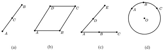
To alleviate combinatorial explosion in geometric reasoning, this paper proposes a merged representation for geometric objects such as lines, planes, and angles, which reduces the number of predicate instantiations required to represent the same geometric knowledge and extends the representation form of geometric objects. Table 1 and Figure 1 summarize the four categories of mergeable geometric objects. Taking collinear points as an example, the traditional representation requires separate predicates $Line(A,B)$, $Line(B,C)$, and $Line(A,C)$ for the same geometric line, whereas the merging representation unifies them into a single $Line(A,B,C)$, eliminating semantic-equivalence redundancy at the representation level. This representation can uniformly characterize structural information such as collinearity, coplanarity, concyclicity, and same-angle edge sets. The general goal of this operation is related to earlier efforts on structured geometric knowledge representation and redundancy control [9]; Table 1 summarizes the object types and merged representations, and Section 4.2 describes the merging procedure.

Table 1. Merging representation of geometric objects.

Mergeable Predicate	Example	Meaning
$Line(p_1,p_2,\dots ,p_n)$	$Line(A,B,C)$	There exists a line $ABC$/points A, B, C are collinear, as in Figure 1a.
$Plane(p_1,p_2,\dots ,p_n)$	$Plane(A,B,C,D)$	There exists a plane $ABCD$/points A, B, C, D are coplanar, as in Figure 1b.
$Angle(V,E_a,E_b)$	$\begin{array}{c}Angle(A,Edge(B,C),\\ Edge(D,E))\end{array}$	Vertex A, with $BC$ on one side and $DE$ on the other side, as in Figure 1c.
$Circle(o,p_1,\dots ,p_n)$	$Circle(O,A,B,C)$	Center O, with A, B, C on the circle, as in Figure 1d.

Figure 1. Geometric objects supporting merged representations: (a) collinear points merged into a line; (b) coplanar points merged into a plane; (c) angle with merged edge sets; (d) circle with multiple points on it. Uppercase letters denote geometric points.

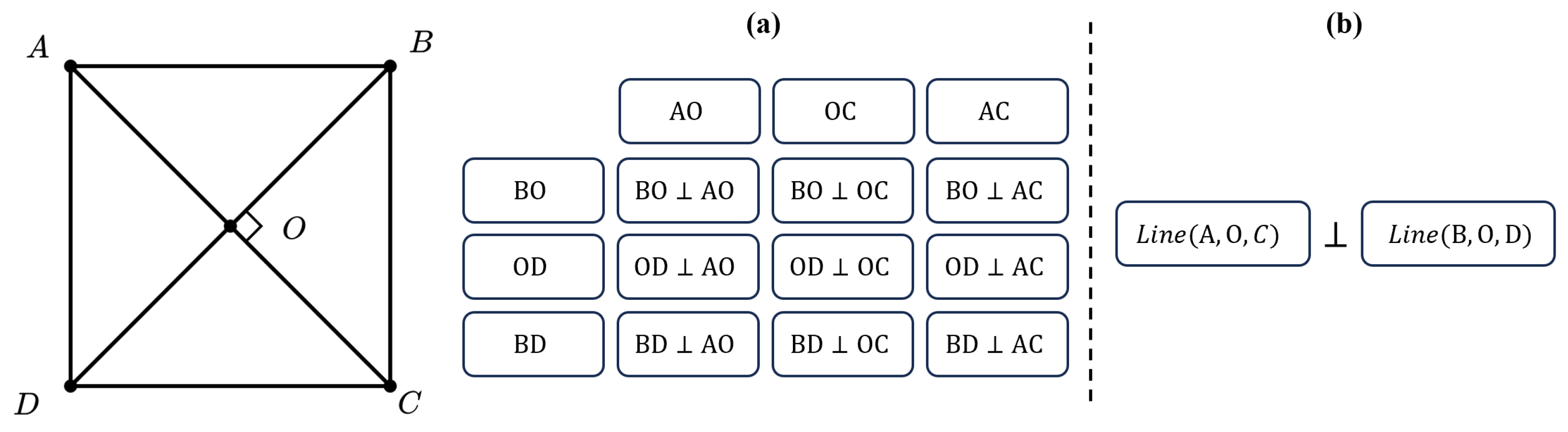
The merged representation of geometric objects not only effectively reduces the number of geometric objects during reasoning but also further reduces the number of geometric relations. Take the mutually perpendicular diagonals of a square as an example, as illustrated in Figure 2. Under the traditional knowledge representation, the diagonals are usually split into $AC$, $AO$, $CO$ and $BD$, $BO$, $DO$. To represent the perpendicular relations between these segments, $3\times 3=9$ pieces of knowledge must be constructed; after adopting the merged representation of lines, these redundant expressions can be unified into a single piece of knowledge, thereby reducing the overhead of knowledge storage and subsequent rule matching.

Figure 2. Illustration of how the line-merging representation compresses redundant perpendicularity relations: (a) traditional representation with nine perpendicularity relations; (b) merged representation with a single perpendicularity relation. Uppercase letters denote geometric points.

The knowledge-merging representation reduces redundant object and relation representations and the associated potential matching space. Rules that compare lines or planes as whole objects can operate directly on the merged representatives; rules requiring individual points or segments can access them through the merged objects.

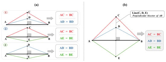
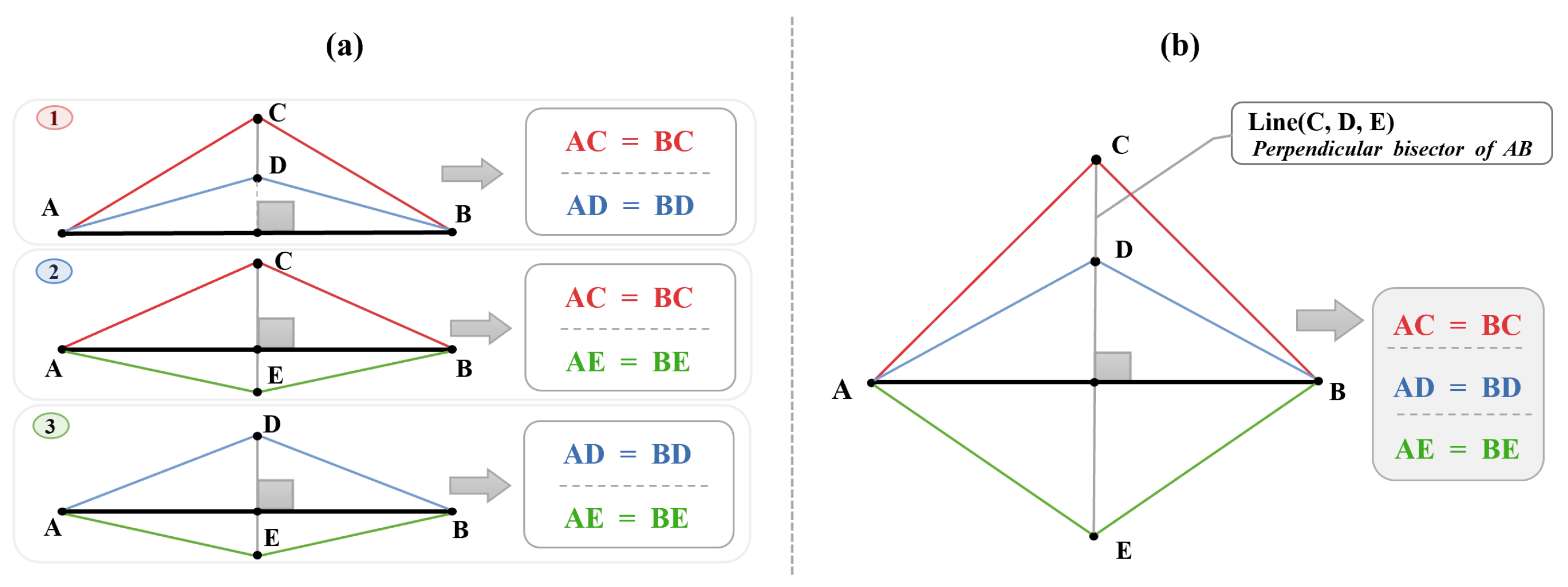
For example, consider the planar rule “two distinct lines perpendicular to the same line are parallel”. A naive matcher that pairs the nine perpendicularity representations in Figure 2 can enumerate up to $C_9^2=36$ raw unordered predicate pairs before shared-variable and geometric compatibility checks. This count is a bound for that pairing strategy. The merged representation removes the redundant predicate pairs at their source. In addition, the merged representation can also reduce the generation of duplicate knowledge among different rule instantiations. As shown in Figure 3, for “line $CDE$ is the perpendicular bisector of segment $AB$”, in the production reasoning regarding “points on the perpendicular bisector are equidistant from the two endpoints”, the traditional representation needs to perform rule instantiation three times for the multiple segment forms on the line and produces six pieces of knowledge, three of which are duplicates; with the merged representation, the rule can directly match the merged line object as a whole, thereby avoiding repeated instantiation for different representations of the same line.

Figure 3. Difference in reasoning for the perpendicular-bisector theorem between the traditional and merged representations: (a) separate matching of segments $CD$, $CE$, and $DE$ produces six equality conclusions, three of which are duplicates; (b) matching the merged line object $Line(C,D,E)$ and iterating over its points yields the three distinct equalities $AC=BC$, $AD=BD$, and $AE=BE$. Uppercase letters denote geometric points.

2.2. Representation of Geometric-Quantity Equality Relations

Geometric reasoning combines deductions about objects and their structural relations with equations for lengths, angles, areas, and ratios. Repeatedly storing equivalent quantitative relations increases both the knowledge-base size and the cost of algebraic solving. This section defines the quantities and equalities used by KM-SCR and introduces a chain representation for their frequent value and ratio relations.

Definition 3 

(Geometric quantity). A geometric quantity is a measurable numerical attribute associated with one or more geometric objects, describing either the intrinsic numerical feature of a single geometric object or the measurable numerical relation among multiple geometric objects. Its formal definition is

$$Q(G_1,\dots ,G_n,type),n\in {\mathbb{N}}^{+}.$$

(4)

Here, $G_1,\dots ,G_n$ are geometric objects, such as triangles, lines, and planes, and $type$ is the specific category of the geometric quantity, such as lengths, distances, angles, and their trigonometric functions.

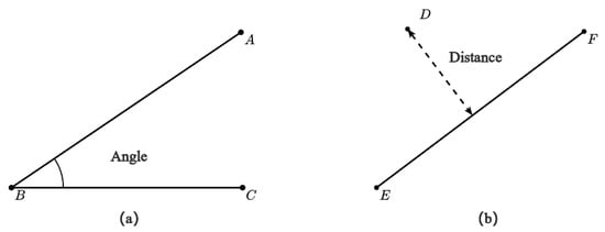
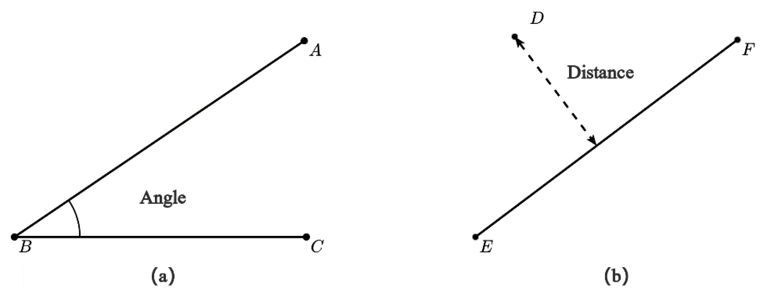
Geometric quantities are used during reasoning to represent the numerical constraints of geometric objects and to participate in subsequent algebraic computation. For example, the magnitude of $\angle ABC$ and the distance from point D to line $EF$ can be formally expressed as $(\angle ABC,\mathit{magnitude})$ and $(D,EF,\mathit{distance})$, respectively, as shown in Figure 4a,b.

Figure 4. Examples of the formal representation of geometric quantities: (a) magnitude of an angle; (b) distance from a point to a line. Uppercase letters denote geometric points.

Definition 4 

(Geometric-quantity equality). A geometric-quantity equality is a formal statement used to express an equality relation among one or more geometric quantities. Its general form is

$$E:Exp{r}_1(Q_1,Q_2,\dots ,Q_n)=Exp{r}_2(Q_1,Q_2,\dots ,Q_n),n\in {\mathbb{N}}^{+}.$$

(5)

Here, $Q_1,Q_2,\dots ,Q_n$ are geometric quantities, and $Exp{r}_1(·)$ and $Exp{r}_2(·)$ are algebraic expressions constructed from these geometric quantities as arguments.

Geometric-quantity equalities provide a basic representation for geometric reasoning and algebraic computation. They are used to describe geometric theorems, constraints, and deduced conclusions, and play a key role in transmitting and generating numerical information during automated reasoning. Geometric-quantity equalities can be classified into the following four special types for differentiated processing; the specific classification and mathematical expressions are shown in Table 2 (for brevity, in the following formulas, a line segment symbol denotes its length, and an angle symbol denotes its measure, unless otherwise specified):

Table 2. Classification of geometric equalities.

Form	Meaning	Example
$Q=C$	QuantityValue ($Qv$)	$AB=5$
$Q_1=C·Q_2$	QuantityRatio ($Qr$)	$AB=2·CD$
$C_1·Q_1+\dots +C_n·Q_n=C$	LinearEquation ($E_{lin}$)	$\angle ABD+\angle DBC-\angle ABC=0$
$Q_1^{e_1}·Q_2^{e_2}\dots ·Q_n^{e_n}=C$	ProductEquation ($E_{prod}$)	${\displaystyle \frac{A{B}^2{S}_{CDE}}{C{D}^2{S}_{ABC}}}=1$

In the process of automated geometry reasoning, the system continuously generates a large number of geometric-quantity equalities. Knowledge discovery on the L6 problems (the highest difficulty level) of the FormalGeo dataset shows that equalities of type $Qv$ and $Qr$ account for 71.62%, occupying the dominant proportion among all geometric-quantity equalities. If these equalities directly participate in reasoning and algebraic computation in discrete form, the representation scale of geometric-quantity relations will grow rapidly and the complexity of equation construction and solving will increase significantly, thereby affecting the overall reasoning efficiency.

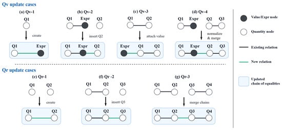
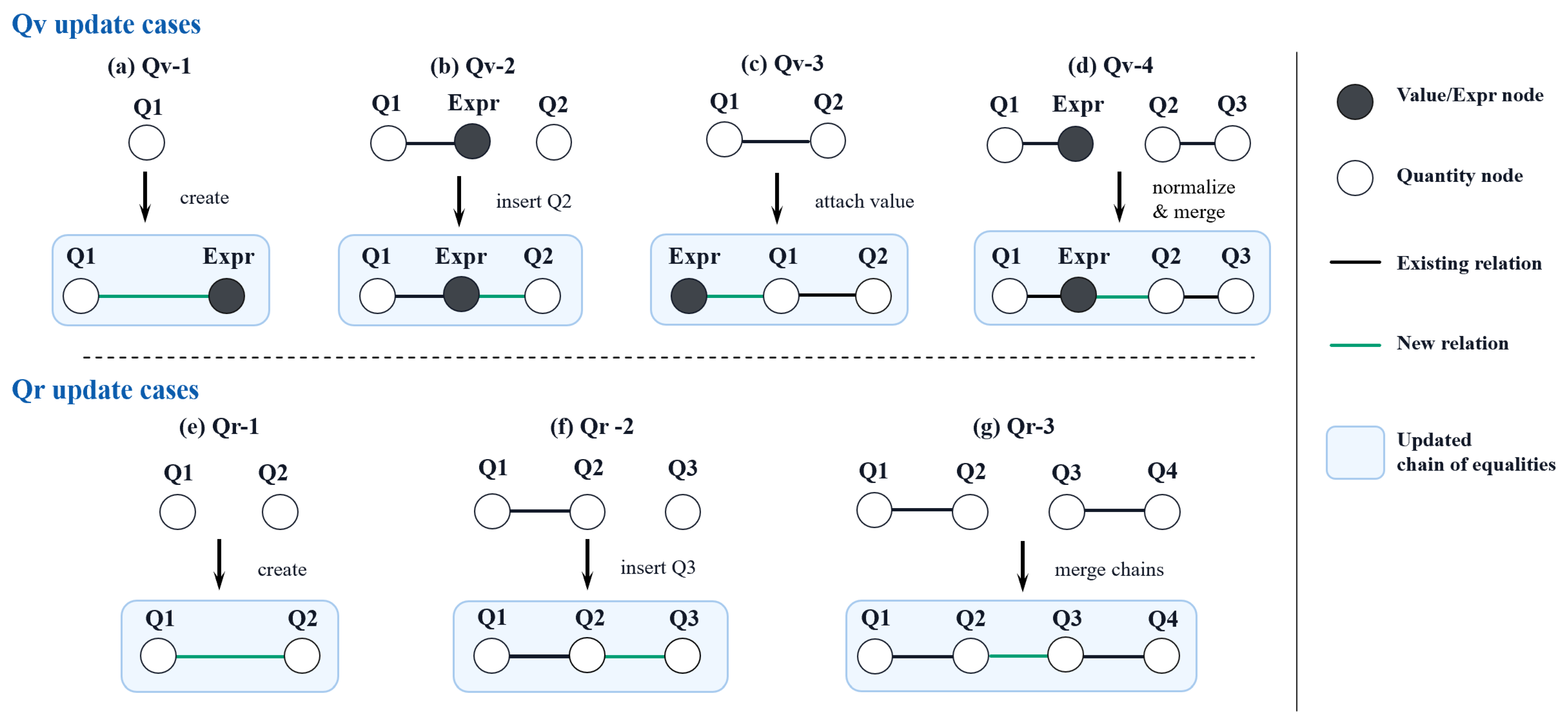
To reduce the redundancy of geometric-quantity equalities at the representation layer, this paper introduces the chain-of-equalities structure, which merges the proportional relations and numerical constraints among multiple geometric quantities into one compact unified representation, so as to reduce the number of equalities and improve the efficiency of subsequent reasoning and computation. The update operations of chains of equalities for different types of newly derived relations are illustrated in Figure 5.

Figure 5. Update operations for chains of equalities for $Qv$ and $Qr$ relations: (a–d) $Qv$ (quantity–value) updates: creating a new chain, extending a chain with an explicit value, assigning a value to an existing chain, and merging chains through an explicit value, respectively; (e–g) $Qr$ (quantity–ratio) updates: creating a new chain, extending an existing chain, and merging two chains, respectively. $Q1$–$Q4$ denote geometric quantities, $Expr$ denotes an explicit numerical expression, and $CE$ denotes a chain of equalities.

Definition 5 

(Geometric chain of equalities). A chain of equalities is used to simultaneously represent the proportional relations among multiple geometric quantities. Its formal definition is

$$CE=\left[(Q_1,C_1),\dots ,(Q_i,C_i)\right],expr,$$

(6)

where $(Q_i,C_i)$ denotes an ordered pair formed by a geometric quantity and its corresponding coefficient, and $expr$ is an optional explicit numerical expression (which may be empty), whose semantics, for nonzero coefficients, are:

$$expr=C_1·Q_1=\dots =C_i·Q_i.$$

(7)

The chain of equalities can directly support the inference of $Qv$- and $Qr$-type geometric-quantity relations. It is also used by the algebraic-reasoning procedures to compress matrix representations, simplify equation systems, and avoid constructing a matrix or equation system for every simple equality combination. Thus, CE is an inference structure as well as a compact representation: its derived equalities can be used as new knowledge in subsequent reasoning, while selected relations can be passed to matrix-based or joint equation-system solving.

In automated geometry reasoning, newly derived geometric-quantity relations are incorporated into the existing chain-of-equalities set to avoid redundant representation and maintain a consistent representation of value and ratio relations. According to the type of the newly generated relation, the update procedure for the chain of equalities also differs.

When a new $Qv$ (quantity–value) relation is derived, the following four cases may occur:

(1)

No existing chain of equalities contains both an explicit value and the geometric quantity in question; in this case, a new chain of equalities containing the explicit value is created, e.g., $CE:AB=5$.

(2)

A chain of equalities containing an explicit value already exists, but no chain of equalities contains the geometric quantity in question, and the newly derived geometric quantity also has an explicit value. In this case, it can be merged into the existing chain of equalities according to the numerical ratio. For example, the system already has $CE:CD=6$, and now derives $AB=2$; the chain of equalities is updated to $CE:3AB=CD=6$.

(3)

A chain of equalities containing the geometric quantity but not an explicit value already exists; the new value is merged into this chain of equalities. For example, the system already has $CE:AB=CD$, and now derives $AB=5$; the value 5 is incorporated into the original chain of equalities: $CE:AB=CD=5$.

(4)

A chain of equalities containing an explicit value exists, and another chain of equalities contains the geometric quantity, indicating that the two describe the same group of numerical relations; in this case, the chain-merging operation is performed. $C{E}_1:AB=CD=5$, $C{E}_2:EF=GH$, and now $EF=10$ is derived; the chains of equalities are merged into $CE:AB=CD=\frac{1}{2}EF=\frac{1}{2}GH=5$.

When a new $Qr$ is derived, the chain-of-equalities update process is relatively simple, and the following three cases may occur:

(1)

Neither geometric quantity appears in any existing chain of equalities; a new chain of equalities is created, e.g., $CE:AB=2CD$.

(2)

Only one geometric quantity already exists in a chain of equalities; the other geometric quantity is added to that chain of equalities. For example, the system already has $CE:CD=EF$, and now derives $2AB=CD$; the chain of equalities is updated to $CE:2AB=CD=EF$.

(3)

The two geometric quantities exist in different chains of equalities, indicating that a mergeable relation exists between the two chains; in this case, the chain-merging operation is performed. For example, the system already has $C{E}_1:AB=CD$ and $C{E}_2:EF=2GH$, and now derives $CD=EF$; they are merged into $CE:AB=CD=EF=2GH$.

Each chain maintains proportional quantities and at most one explicit value. Traversing it yields further $Qv$ and $Qr$ relations for subsequent reasoning. If a new relation involves quantities already in the same chain, it is checked against the existing coefficients; a consistent relation leaves the chain unchanged. Zero-valued quantities require direct value handling whenever a merge would involve division by zero.

3. Semi-Conditional Rule Representation

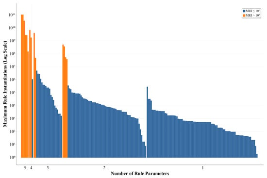
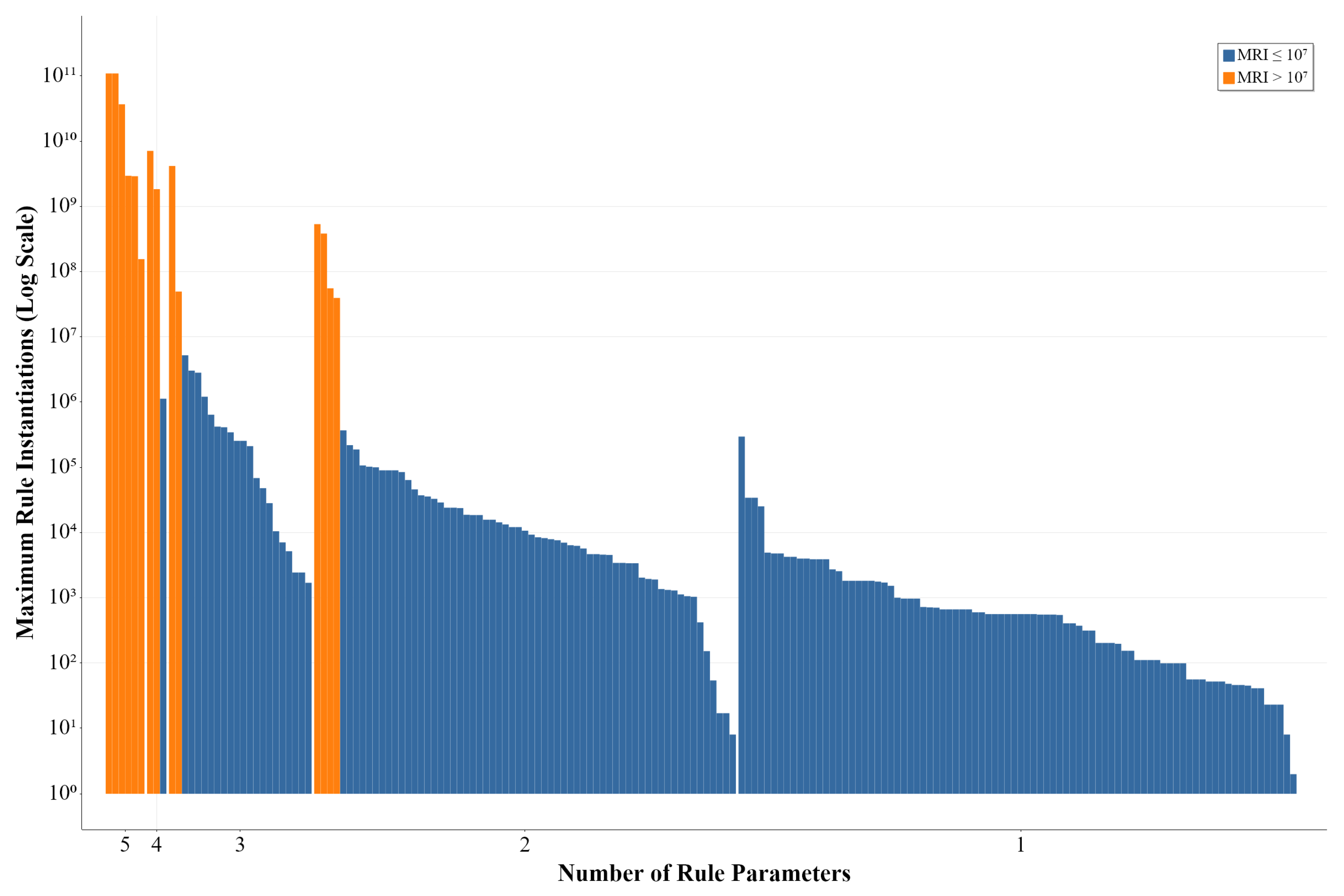
Rules with many antecedents can have large Cartesian-product matching spaces. Figure 6 summarizes the MRI values computed by Equation (1) from knowledge accumulated to the reasoning fixed point on FormalGeo7k-L6. The orders-of-magnitude differences motivate separating conditions that determine a candidate from conditions that verify it.

Figure 6. Maximum possible number of rule instantiations (MRI) computed by Equation (1) for each rule category on the FormalGeo7k-L6 dataset. The x-axis denotes the number of rule parameters, and the y-axis uses a logarithmic scale due to the large range of instantiation counts.

In a full-antecedent formulation, each antecedent contributes to the potential matching combinations. Many geometric rules admit a smaller set of base conditions that determines the candidate objects and their correspondences. The remaining predicates can then be checked for that candidate. Semi-conditional rules formalize this separation and retain pending candidates across inference rounds. A candidate whose remaining constraints are not yet established is maintained as a pending instance for verification when relevant facts become available.

Definition 6 

(Rule). A rule is a logical statement that specifies relationships among predicates or defines how predicate conditions imply new facts, such as a geometric theorem, axiom, definition, lemma, formula, law, or corollary. Formally, a rule is denoted by r (and a rule set by $\mathcal{R}$), written as

$$r:p_1\wedge \dots \wedge p_n\to c_1,\dots ,c_m,n,m\in \mathbb{N}.$$

(8)

Here, $p_1,\dots ,p_n$ are the antecedent conditions of the rule, and $c_1,\dots ,c_m$ are the conclusions of the rule. A rule is usually described in the form “if…, then…”, where the “if” part corresponds to the conditions and the “then” part corresponds to the conclusions, which are logically derived from the conditions. For example, the transitivity of line parallelism can be represented by the rule:

$$\begin{array}{c}\hfill Parallel(l_1,l_2)\wedge Parallel(l_2,l_3)\to Parallel(l_1,l_3).\end{array}$$

(9)

Definition 7 

(Semi-conditional rule). Consider a multi-condition rule containing two or more antecedent conditions:

$$r:p_1\wedge \dots \wedge p_N\to H,N\ge 2,$$

(10)

if its antecedent conditions can be partitioned into base conditions B and constraint conditions C, where

$$\begin{array}{cc}\hfill B& =p_1\wedge \dots \wedge p_k,\hfill \end{array}$$

(11)

$$\begin{array}{cc}\hfill C& =p_{k+1}\wedge p_{k+2}\wedge \dots \wedge p_N,1\le k<N,\hfill \end{array}$$

(12)

then the corresponding semi-conditional rule is written as:

$$r_s:B⇝⟨C,H⟩.$$

(13)

Here, B denotes the base conditions used to generate candidate rule instances, whereas C denotes the constraint conditions that are verified after a candidate has been generated. The base match must bind every variable in C and H, including any explicitly enumerated object correspondences. This requirement makes each pending constraint a fully instantiated predicate. The conclusion H is derived when all predicates in C are satisfied.

Proposition 1 

(Per-application equivalence). Let an admissible rule be written as $B\wedge C\to H$, and let its semi-conditional form be $B⇝⟨C,H⟩$. For any knowledge base $\mathcal{K}$ and variable substitution θ, the original rule is applicable under θ if and only if the candidate generated from $B\theta$ is accepted after all predicates in $C\theta$ have been verified against $\mathcal{K}$.

Proof. 

The original rule is applicable under $\theta$ exactly when $B\theta \subseteq \mathcal{K}$ and $C\theta \subseteq \mathcal{K}$. The semi-conditional procedure generates a candidate from $B\theta$ and accepts it only when every predicate in $C\theta$ is present in $\mathcal{K}$. Hence,

$$r\mathrm{is}\mathrm{applicable}\mathrm{under}\theta \iff B\theta \subseteq \mathcal{K}\wedge C\theta \subseteq \mathcal{K}\iff r_s\mathrm{accepts}\mathrm{the}\mathrm{candidate}\mathrm{under}\theta .$$

(14)

Once accepted, both representations derive the same conclusion $H\theta$. Thus, the semi-conditional representation preserves the applicability and conclusion of each individual rule instance.    □

Proposition 1 establishes equivalence at the rule-instance level. At the inference-process level, this equivalence is preserved provided that object merging maintains the geometric facts represented by the affected objects, and that pending rule instances are rechecked when their remaining conditions become available. Thus, although merging may replace previously represented objects with their merged representatives, it does not change the logical content of the corresponding facts. Consequently, each accepted semi-conditional instance satisfies the premises of the original rule.

For example, the side–side–side ($SSS$) triangle-congruence rule can be written as $B\wedge C\to H$, with the two triangle objects as base conditions and the three corresponding side equalities as constraints:

$$\begin{array}{cc}\hfill B& =Tri(A,B,C)\wedge Tri(D,E,F),\hfill \end{array}$$

(15)

$$\begin{array}{cc}\hfill C& =SegEq(AB,DE)\wedge SegEq(BC,EF)\wedge SegEq(AC,DF),\hfill \end{array}$$

(16)

$$\begin{array}{cc}\hfill H& =TCE(ABC,DEF).\hfill \end{array}$$

(17)

Accordingly, the rule instantiation under the semi-conditional rule representation is:

$$r_s^{CongSSS}:Tri(A,B,C)\wedge Tri(D,E,F)⇝⟨C,TCE(ABC,DEF)⟩.$$

(18)

When the system matches the base conditions $Tri(A,B,C)$ and $Tri(D,E,F)$, it does not immediately derive the triangle-congruence conclusion, but instead generates and records the corresponding “constraint-condition–candidate-conclusion” pair:

$$SegEq(AB,DE)\wedge SegEq(BC,EF)\wedge SegEq(AC,DF)\to TCE(ABC,DEF),$$

(19)

as well as the remaining symmetric cases generated by the point correspondences. During reasoning, when the corresponding constraint conditions are gradually satisfied, the system marks their status as satisfied; when all the constraint conditions in the group are satisfied, the corresponding conclusion is added to the knowledge base.

Semi-conditional rules can be applied to the rewriting of geometric theorems containing multiple categories of antecedent conditions. Typical examples include the judgments of special quadrilaterals (parallelogram, rectangle, rhombus), the congruence and similarity judgments of triangles, and the properties of angle bisectors (i.e., points on an angle bisector are equidistant from the two sides of the angle).

Example 1. 

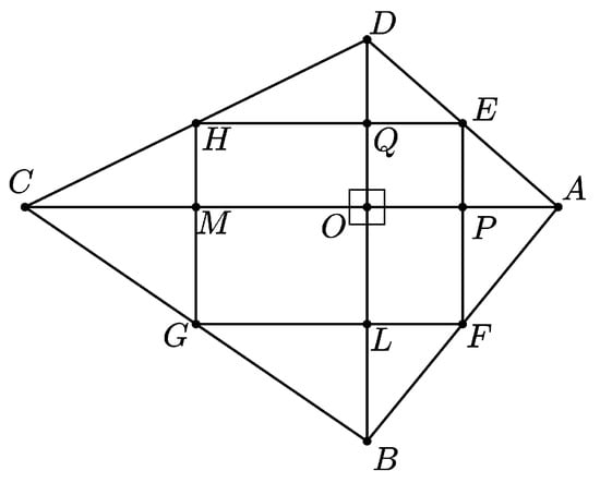
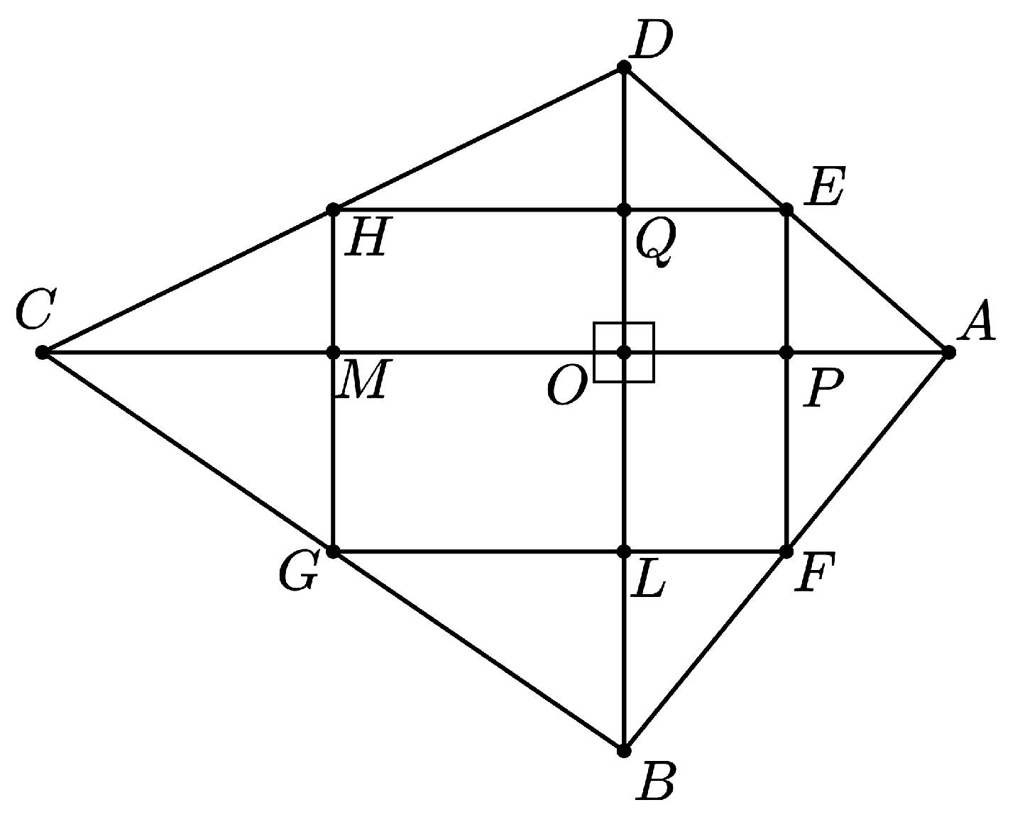
As shown in Figure 7, $AC=10$, $BD=6$, E is the midpoint of segment $AD$, F is the midpoint of segment $AB$, G is the midpoint of segment $BC$, H is the midpoint of segment $CD$, $AO\perp BO$, $BO\perp CO$, $CO\perp DO$, and $DO\perp AO$. Find the area of quadrilateral $EHGF$.

Figure 7. Reference diagram for problem 3616 from the FormalGeo7k dataset.

Under the traditional knowledge-representation framework, the system can discover, through deductive reasoning, 34 groups of segment-equality relations, 20 triangle objects, and 2072 angle-equality predicate instantiations. If the Angle-Angle-Side (AAS) congruence judgment rule is applied directly, the maximum instantiation search space can reach $20\times 20\times 2072\times 2072\times 34=5.84\times {10}^{10}$ before shared-variable and geometric compatibility checks.

With semi-conditional rules, the two triangle predicates contribute $20\times 20=400$ base-object pairs. Enumerating six vertex correspondences for each pair gives 2400 candidate constraint–conclusion records. The backward index retrieves these records as their required equalities become available. This example illustrates the reduction from a full-antecedent Cartesian-product bound to a base-pair candidate space; Section 5 separately reports measured inference costs.

4. KM-SCR: An Automated Geometry Reasoning System

The preceding sections introduced three complementary mechanisms: geometric-object merging, chains of equalities, and semi-conditional rules. Geometric-object merging reduces redundant object and relation representations, semi-conditional rules defer the verification of remaining conditions until necessary, and chains of equalities facilitate quantitative inference and provide algebraic relations for equation-system reasoning.

We integrate these mechanisms into an iterative deductive-database reasoning algorithm and develop KM-SCR (Knowledge Merging and Semi-Conditional Rules), an automated geometry reasoning system. The system aims to improve inference efficiency by reducing redundant representations and unnecessary rule-matching operations while preserving the geometric and algebraic information required for subsequent reasoning.

4.1. System Architecture of KM-SCR

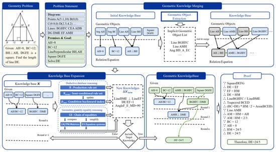
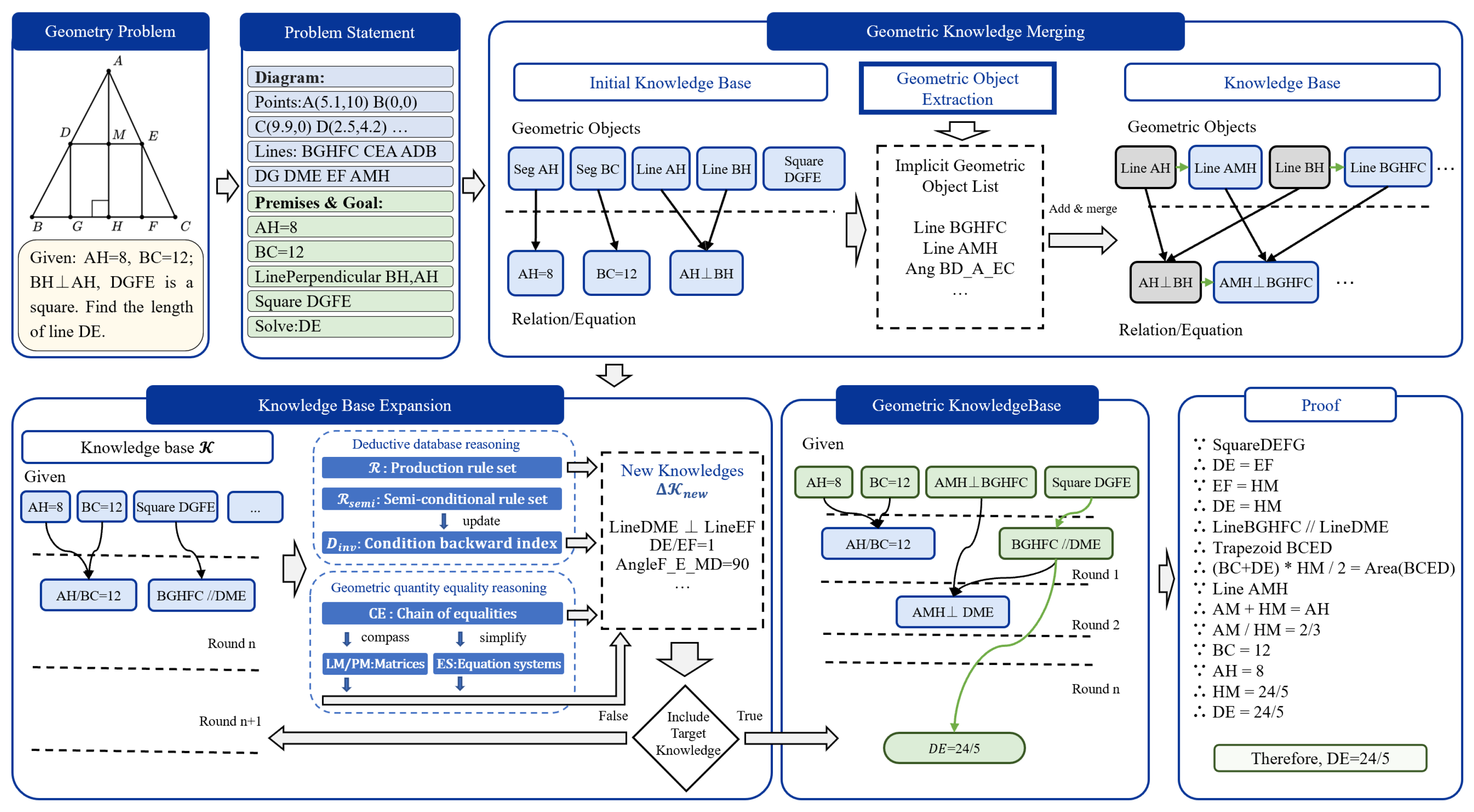
As illustrated in Figure 8, KM-SCR first constructs an initial knowledge base by parsing the given geometric conditions. It then identifies and merges equivalent geometric objects to obtain a more compact representation. The reasoning process proceeds iteratively, applying production rules, semi-conditional rules, chains of equalities, and equation-system reasoning to derive new geometric knowledge. Newly discovered knowledge is incorporated into the knowledge base, and the process continues until the target is established or no further knowledge can be derived. Once the target is established, the system traces the recorded dependencies backward and topologically orders the corresponding deductions to generate a readable solution. Complete reconstruction of matrix-derived reasoning paths remains a direction for future work.

Figure 8. Overall workflow of the KM-SCR automated geometry reasoning system, including knowledge-base construction, geometric-object merging, iterative logical and algebraic inference, and solution generation. Diagram coordinates support structural checks, such as point ordering; metric lengths are derived from the symbolic premises rather than measured from the diagram. Ellipses indicate additional geometric objects, relations, equations, or derived knowledge omitted for visual clarity.

4.2. Geometric-Object Mining and Merging Algorithm

To improve the efficiency and consistency of geometric knowledge representation, we propose a geometric-object mining and merging algorithm (Algorithm 1). The algorithm identifies mergeable objects as new geometric knowledge is derived and propagates each merge to the affected relations. When a new object is introduced, the algorithm searches the current knowledge base for objects that can be represented by the same normalized object, constructs the merged representation, and updates the associated relations accordingly. This process preserves the represented geometric information while reducing redundant objects and relations, thereby providing a more compact knowledge base for subsequent logical and algebraic reasoning.

Definition 8. 

A knowledge base ($\mathcal{K}$) is represented as a triple ($\mathcal{K}=⟨G,F,E⟩$), where $G=\{G_1,G_2,\dots ,G_{n_1}\}$ is the set of geometric objects (such as points, lines, faces, circles, etc.); $F=\{F_1,F_2,\dots ,F_{n_2}\}$ is the set of geometric relations (such as collinearity, coplanarity, parallelism, etc.); and $E=\{E_1,E_2,\dots ,E_{n_3}\}$ is the set of algebraic equalities of geometric quantities.

Algorithm 1 Geometric-Object Mining and Merging

Require:  Current knowledge base $\mathcal{K}$, mining rule set ${\mathcal{R}}^{dig}$. Ensure:  Updated knowledge base ${\mathcal{K}}^{\prime }$.   1: ${\mathcal{K}}^{\prime }\leftarrow \mathcal{K}$   2: for all $⟨r,{\mathcal{K}}_{match}⟩\in Match(\mathcal{K},{\mathcal{R}}^{dig})$ do   3:       $F_{der}\leftarrow r.Execute({\mathcal{K}}_{match})$   4:       for all $f\in F_{der}$ do   5:             $⟨g_{new},G_{base}⟩\leftarrow FindAndMergeObjects({\mathcal{K}}^{\prime },f)$   6:             $⟨F_{new},F_{base}⟩\leftarrow FindRelations({\mathcal{K}}^{\prime },g_{new},G_{base})$   7:             Mark $G_{base}$ and $F_{base}$ as inactive   8:             Add $g_{new}$ and $F_{new}$ to ${\mathcal{K}}^{\prime }$   9:       end for 10: end for 11: return ${\mathcal{K}}^{\prime }$

The algorithms use three generic engine operations: $Match$ returns rule substitutions satisfying the matched antecedents, $Execute$ constructs the instantiated conclusions or pending records, and $IsSatisfied$ tests all instantiated constraints against the current knowledge. For semi-conditional rules, $Match$ operates on the base conditions. The representation-specific operations are described alongside their use below.

First, the algorithm uses the matching function $Match$ to instantiate the mining rule set ${\mathcal{R}}^{dig}$ against the current knowledge base $\mathcal{K}$ and execute rule deduction (lines 2–3). The mining rules aim to capture implicit geometric objects from the existing geometric constraint structure; for example, from the fact that A is the midpoint of $BC$, the system can deduce that A, B, and C are collinear and generate a new $Line(A,B,C)$ geometric object.

For each candidate object, $FindAndMergeObjects$ returns the merged representation and its base objects (lines 4–5). Given the candidate object f, this function searches the current geometric-object set for all objects that can be merged with f according to the corresponding object-type and normalization rules, and collects them into $G_{base}$. It then constructs the normalized merged object $g_{new}$ from $\{f\}\cup G_{base}$. For example, when a newly derived line $Line(A,C,M)$ overlaps an existing line $Line(C,M,D)$, the two objects can be represented by the merged line $g_{new}$ representing $Line(A,C,M,D)$, while the original objects are retained as the base-object set $G_{base}$. For a line, two distinct common points establish identity and the point sets are united. Angle merging preserves the vertex and the two edges; circle merging preserves the defining circle. A merge can expose further equivalent objects, so the search continues until no further object joins the merged representation.

Finally, the state-update stage applies the merge to the knowledge base (lines 7–9). The base objects $G_{base}$ and their associated relations $F_{base}$ are marked as inactive, while the merged object $g_{new}$ is added as an active object and the updated relations $F_{new}$ are added to ${\mathcal{K}}^{\prime }$. Each updated relation is obtained by replacing references to objects in $G_{base}$ with the merged representative $g_{new}$. This update preserves the represented geometric facts while maintaining consistent references to the merged objects. The resulting knowledge base ${\mathcal{K}}^{\prime }$ provides a more compact representation for subsequent deductive-database reasoning. The relation replacement step is formalized in Algorithm 2.

Algorithm 2 Relation propagation during object merging

Require:  Knowledge base $\mathcal{K}$, merged object $g_{new}$, base-object set $G_{base}$. Ensure:  Updated relation set $F_{new}$ and replaced relation set $F_{base}$.   1: $F_{base}\leftarrow \{f\in \mathcal{K}.F\mid Objects(f)\cap G_{base}\ne \varnothing \}$   2: $F_{new}\leftarrow \varnothing$   3: for all $f\in F_{base}$ do   4:       $F_{new}\leftarrow F_{new}\cup \{Replace(f,G_{base},g_{new})\}$   5: end for   6: return $F_{new},F_{base}$

4.3. Deductive-Database Reasoning Algorithm

Algorithm 3 implements the deductive-reasoning block in the lower-left panel of Figure 8. Its five inputs describe the inference state: $\mathcal{K}$ holds the current facts; $\mathcal{R}$ and ${\mathcal{R}}_{semi}$ supply ordinary and semi-conditional rules; $D_{inv}$ stores pending candidates; and $\mathsf{\Delta }{\mathcal{K}}_{prev}$ carries the preceding round’s discoveries. In the figure, $\mathsf{\Delta }{\mathcal{K}}_{new}$ becomes the next round’s increment. Each index entry $D_{inv}[c]$ contains records $⟨C,H⟩$ awaiting the instantiated predicate c, with C retaining the complete deferred-condition set.

Algorithm 3 Deductive-Database Reasoning

Require:  Current knowledge base $\mathcal{K}$, rule set $\mathcal{R}$, semi-conditional rule set ${\mathcal{R}}_{semi}$, backward index $D_{inv}$, previous-round new knowledge $\mathsf{\Delta }{\mathcal{K}}_{prev}$. Ensure:  New knowledge set $\mathsf{\Delta }{\mathcal{K}}_{new}$, updated backward index $D_{inv}^{\prime }$.   1: ${\mathcal{K}}^{\prime }\leftarrow \mathcal{K}\cup \mathsf{\Delta }{\mathcal{K}}_{prev},D_{inv}^{\prime }\leftarrow D_{inv},\mathsf{\Delta }{\mathcal{K}}_{new}\leftarrow \varnothing$   2: for all $⟨r,{\mathcal{K}}_{match}⟩\in Match({\mathcal{K}}^{\prime },\mathcal{R})$ do   3:       $F_{new}\leftarrow r.Execute({\mathcal{K}}_{match})$   4:       $\mathsf{\Delta }{\mathcal{K}}_{new}\leftarrow \mathsf{\Delta }{\mathcal{K}}_{new}\cup F_{new}$   5: end for   6: for all $⟨r,{\mathcal{K}}_{match}⟩\in Match({\mathcal{K}}^{\prime },{\mathcal{R}}_{semi})$ do   7:       $⟨C,H⟩\leftarrow r.Execute({\mathcal{K}}_{match})$   8:       if $IsSatisfied(C,{\mathcal{K}}^{\prime })$ then   9:             $\mathsf{\Delta }{\mathcal{K}}_{new}\leftarrow \mathsf{\Delta }{\mathcal{K}}_{new}\cup \{H\}$ 10:       else 11:             for all $c\in C\setminus {\mathcal{K}}^{\prime }$ do 12:                   $D_{inv}^{\prime }[c]\leftarrow D_{inv}^{\prime }[c]\cup \{⟨C,H⟩\}$ 13:             end for 14:       end if 15: end for 16: for all $f_{prev}\in \mathsf{\Delta }{\mathcal{K}}_{prev}$ do 17:       for all $⟨C,H⟩\in D_{inv}^{\prime }[f_{prev}]$ do 18:             if $IsSatisfied(C,{\mathcal{K}}^{\prime })$ then 19:                   $\mathsf{\Delta }{\mathcal{K}}_{new}\leftarrow \mathsf{\Delta }{\mathcal{K}}_{new}\cup \{H\}$ 20:             end if 21:       end for 22: end for 23: return $\mathsf{\Delta }{\mathcal{K}}_{new}\setminus {\mathcal{K}}^{\prime },D_{inv}^{\prime }$

The algorithm first forms the current snapshot ${\mathcal{K}}^{\prime }=\mathcal{K}\cup \mathsf{\Delta }{\mathcal{K}}_{prev}$. Ordinary rules add their instantiated conclusions to the output set. Semi-conditional rules generate $⟨C,H⟩$ records: a fully satisfied record contributes H immediately, while a pending record is indexed under each missing predicate. The preceding round’s new facts also retrieve existing records for verification against the same snapshot. Set-valued outputs suppress duplicate conclusions, and facts already in ${\mathcal{K}}^{\prime }$ are excluded from the returned increment.

Consider Problem in Figure 8. From the properties of the inscribed square $DGFE$ and the perpendicular relations, the system derives $DE=EF$, identifies $MHFE$ as a rectangle, and obtains $EF=HM$, hence $DE=HM$. The parallel relation $DE\Vert BC$, together with the common angle $\angle DAE=\angle BAC$, provides the basis for establishing $▵ADE\sim ▵ABC$ once the required corresponding-angle condition is verified. The similarity relation then yields $AM/AH=DE/BC$, which, combined with $AH=8$, $BC=12$, and $DE=HM$, gives $AM={\displaystyle \frac{2}{3}}HM$. Using $AM+HM=AH$, the system obtains $DE=HM={\displaystyle \frac{24}{5}}$.

This example also illustrates the role of semi-conditional rules. During rule matching, the common-angle relation and the parallelism-derived angle relation can satisfy part of the similarity rule’s antecedent, while the remaining required condition may not yet be available. The corresponding rule instance is retained in the backward index and reconsidered when new knowledge is derived. The similarity conclusion is produced only after the complete antecedent is verified. Thus, semi-conditional matching preserves potentially useful partial matches without treating them as established geometric conclusions.

4.4. Product-Matrix Representation and Implicit-Knowledge Extraction Mechanism

For positive quantities and a positive right-hand side, a product equality ${\prod }_i{Q}_i^{e_i}=c$ becomes ${\sum }_i{e}_i\log Q_i=\log c$. This transformation permits linear elimination; related algebraic reasoning is used in AlphaGeometry2 [26]. KM-SCR uses an explicit product matrix ($Pm$) to expose the resulting value and ratio relations to subsequent deductive reasoning. Equations outside the positive domain are retained for equation-system solving.

The $CompassByCE$ operation substitutes the representative quantity of each equality chain and combines the corresponding matrix columns. If $C_i{Q}_i=C_r{Q}_r$, the substitution is $Q_i=(C_r/C_i)Q_r$. For a linear matrix, coefficients are rescaled and added; for a product matrix, exponents are added and the proportional factors are transferred to the right-hand side. Known values are substituted directly. Thus, compression reduces the matrix dimension while preserving the represented equations on their admissible domain.

$Matrix.Discover(M)$ takes the compressed augmented matrix and returns $Qv$ and $Qr$ facts after row reduction. For $Pm$, the reduced rows are interpreted as equations in logarithmic variables. The extraction uses two operations:

• Intra-row scanning: traverse the simplified matrix row vectors and directly extract basic geometric relations according to the distribution of non-zero elements. For a product-matrix row $a\log Q_i=d$, emit $Q_i=\exp (d/a)$. For a row $a\log Q_i-a\log Q_j=d$, emit $Q_i=\exp (d/a)Q_j$. For $Lm$, the corresponding patterns are $a{Q}_i=d$ and $a{Q}_i+b{Q}_j=0$, yielding $Q_i=d/a$ and $Q_i=-(b/a)Q_j$, respectively. All divisions require nonzero divisors.
• Inter-row computation: compare reduced rows and cancel proportional coefficient patterns on their shared variables. Apply the same value/ratio tests to the residual equation and emit the resulting relations. This extracts ratios exposed by cancellation, as illustrated below.

In Figure 9, merging the $AB$ and $BC$ columns removes a redundant value equation. Intra-row extraction gives $CD/EF=1/2$, $DE/EF=1$, and $BC=5$. Subtracting the two logarithmic ratio rows eliminates $\log EF$ and yields $CD/DE=1/2$. These extracted relations return to the deductive knowledge base.

Figure 9. Product-matrix compression using $AB=BC$. Columns contain exponents; RHS displays the original multiplicative constants (their logarithms enter linear elimination). The compressed matrix yields $CD/EF=1/2$, $DE/EF=1$, and $BC=5$.

4.5. Geometric-Quantity Equality Reasoning Algorithm

Building on the product-matrix representation and implicit-knowledge extraction mechanism described above, this section integrates the algebraic representations into a unified geometric-quantity equality reasoning algorithm. $Qv$ and $Qr$ relations are maintained in the chain-of-equalities set ($CE$) and can directly generate further quantitative knowledge. Linear equalities ($E_{lin}$) and product equalities ($E_{prod}$) are maintained in the linear matrix ($Lm$) and product matrix ($Pm$), respectively. The $CE$ relations are used to compress matrix columns and to simplify candidate equation systems. Equalities that cannot be directly incorporated into these matrix representations are maintained in the equation-system set ($ES$) for subsequent joint solving. Let $ES=\{{\epsilon }_1,{\epsilon }_2,\dots ,{\epsilon }_n\}$ be the maintained set of candidate equation systems, where each ${\epsilon }_i$ is formed by pairing one or two geometric-quantity equalities.

Algorithm 4 first inserts new equalities by type and constructs candidate local systems. It then extracts chain relations, compresses the matrices, and simplifies the local systems before solving.

Algorithm 4 Geometric-Quantity Equality Reasoning

Require:  Current knowledge base $\mathcal{K}$, previous-round new knowledge $\mathsf{\Delta }{\mathcal{K}}_{prev}$, linear matrix $Lm$, product matrix $Pm$, chain-of-equalities set $CE$, equation-system set $ES$. Ensure:  New knowledge set $\mathsf{\Delta }{\mathcal{K}}_{new}$, new linear matrix $L{m}^{\prime }$, new product matrix $P{m}^{\prime }$, new chain-of-equalities set $C{E}^{\prime }$, new equation-system set $E{S}^{\prime }$.   1: $\mathsf{\Delta }{\mathcal{K}}_{new}\leftarrow \varnothing$, $L{m}^{\prime }\leftarrow Lm$, $P{m}^{\prime }\leftarrow Pm$, $C{E}^{\prime }\leftarrow CE$, $E{S}^{\prime }\leftarrow ES$   2: for all $e\in \mathsf{\Delta }{\mathcal{K}}_{prev}\mid e\in Qv\cup Qr$ do   3:       $C{E}^{\prime }\leftarrow UpdateCE(C{E}^{\prime },e)$   4: end for   5: for all $e\in \mathsf{\Delta }{\mathcal{K}}_{prev}\mid e\in E_{lin}$ do   6:       $L{m}^{\prime }\leftarrow L{m}^{\prime }\cup \{e\}$   7:       $E{S}^{\prime }\leftarrow E{S}^{\prime }\cup \{\{e,p\}\mid p\in \mathcal{K}.E\setminus E_{lin}\}\cup \{\{e\}\}$   8: end for   9: for all $e\in \mathsf{\Delta }{\mathcal{K}}_{prev}\mid e\in E_{prod}$ do 10:       $P{m}^{\prime }\leftarrow P{m}^{\prime }\cup \{e\}$ 11:       $E{S}^{\prime }\leftarrow E{S}^{\prime }\cup \{\{e,p\}\mid p\in \mathcal{K}.E\setminus E_{prod}\}\cup \{\{e\}\}$ 12: end for 13: for all $e\in \mathsf{\Delta }{\mathcal{K}}_{prev}.E\setminus (Qv\cup Qr\cup E_{lin}\cup E_{prod})$ do 14:       $E{S}^{\prime }\leftarrow E{S}^{\prime }\cup \{\{e,p\}\mid p\in \mathcal{K}.E\}\cup \{\{e\}\}$ 15: end for 16: $\mathsf{\Delta }{\mathcal{K}}_{new}\leftarrow \mathsf{\Delta }{\mathcal{K}}_{new}\cup C{E}^{\prime }.Discover()$ 17: $L{m}^{\prime }\leftarrow L{m}^{\prime }.CompassByCE(C{E}^{\prime }),P{m}^{\prime }\leftarrow P{m}^{\prime }.CompassByCE(C{E}^{\prime })$ 18: $\mathsf{\Delta }{\mathcal{K}}_{new}\leftarrow \mathsf{\Delta }{\mathcal{K}}_{new}\cup Matrix.Discover(L{m}^{\prime })\cup Matrix.Discover(P{m}^{\prime })$ 19: for all $\epsilon \in E{S}^{\prime }$ do 20:       $\epsilon \leftarrow \epsilon .SimplifyByCE(C{E}^{\prime })$ 21:       $\mathsf{\Delta }{\mathcal{K}}_{new}\leftarrow \mathsf{\Delta }{\mathcal{K}}_{new}\cup \epsilon .Solve()$ 22: end for 23: return $\mathsf{\Delta }{\mathcal{K}}_{new}\setminus (\mathcal{K}\cup \mathsf{\Delta }{\mathcal{K}}_{prev}),L{m}^{\prime },P{m}^{\prime },C{E}^{\prime },E{S}^{\prime }$

Insertion and pairing. $UpdateCE$ applies the chain-update cases of Section 2.2 to each new $Qv$ or $Qr$ fact. Linear and product equations are inserted into their respective matrices. Local systems contain a single equation or a pair; new linear equations are paired with existing non-linear-type equations, and new product equations with existing non-product-type equations. The matrices handle combinations within their respective classes, reducing redundant local solving.

Chain discovery. $CE.Discover$ takes the updated chains and returns their implied value and ratio facts. For a chain $C_1{Q}_1=\cdots =C_k{Q}_k=v$, it emits $Q_i=v/C_i$ when v is known and $Q_i=(C_j/C_i)Q_j$ for pairs of quantities. Without an explicit value, only the ratio relations are emitted. Relations are normalized and deduplicated before insertion into the knowledge base.

Matrix discovery. $CompassByCE$ returns the compressed $Lm$ and $Pm$ matrices using the substitutions described in Section 4.4. $Matrix.Discover$ then performs the row reduction and value/ratio extraction specified there.

Equation-system simplification. $\epsilon .SimplifyByCE(CE)$ takes a candidate equation system and the current chains, and returns an equivalent system under those chain relations. It identifies quantities in the equations, selects a representative from each relevant chain, substitutes proportional quantities and known values, and simplifies the resulting expressions. Where the solver requires explicit equations, representative-to-member equalities encode the same substitutions. $Solve$ processes the reduced system and returns quantitative relations valid under the geometric domain constraints; ambiguous solution branches require further constraints. The representative mappings translate derived results back to the original quantities.

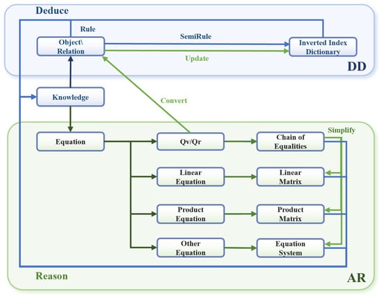
Figure 10 summarizes the exchange between the logical and algebraic modules. Rule conclusions update the chains, matrices, and local equation systems; extracted quantitative relations return as facts for subsequent rule matching. These modules share the same incremental knowledge-base update cycle.

Figure 10. Knowledge-flow relationships between the logical-reasoning level (predicate knowledge, semi-conditional rules, object merging) and the algebraic-computation level (chains of equalities, linear matrix, product matrix, equation systems) in the KM-SCR system.

5. Experimental Results and Analysis

To evaluate KM-SCR across different problem difficulties, we construct an evaluation set of 493 FormalGeo7k instances. We randomly sample 40 problems from each of levels L1–L5 using a fixed random seed (42) and include all 293 problems from L6, which comprises problems with reasoning-path lengths of at least 11. This design provides cross-level evaluation and a comprehensive stress test on the highest difficulty level. FormalGeo7k offers broad plane-geometry coverage, while its longer-path problems require deeper combinations of intermediate deductions and inference rules. All KM-SCR experiments use a timeout of 600 s per problem. The experiments were conducted on a computing platform equipped with an AMD Ryzen 9 9950X processor.

5.1. Comparison of Problem-Solving Performance

Table 3 reports the problem-solving success rate (PSSR) on L6 and the source of each result. KM-SCR solves 288 of 293 instances (98.29%), the locally reproduced FormalGeo FW-BFS baseline solves 17 (5.80%), and the locally reproduced FGeo-NSS achieves 60.41%. KM-SCR and the locally reproduced baselines were evaluated on the same computing platform, using the same 293 L6 problems, a 600 s timeout per problem, and the same success criterion. For the baselines, modifications were confined to the evaluation code; their inference procedures, rule sets, and reasoning-related preprocessing were retained. The local comparison evaluates the systems with their respective rule coverage and implementations; the observed performance differences therefore reflect system-level performance.

Table 3. L6 problem-solving success rates and background references. Local runs use the complete 293-instance subset and a 600 s timeout. Published reference values retain the evaluation protocols of the cited source.

Method	PSSR	Result Source
FW-BFS [19]	5.80%	Local reproduction
FGeo-DRL [37]	39.62%	Published reference [23]
FGeo-HyperGNet	58.82%	Published reference [23]
FGeo-NSS [23]	60.41%	Local reproduction
KM-SCR (Ours)	98.29%	Present work

The published FGeo-DRL and FGeo-HyperGNet results are included as contextual references and retain the evaluation protocols of their original sources.

5.2. Cross-Level Performance and Computational Cost

We report four realized-cost measures. Solving success counts the problems whose target is derived within the timeout. Solving time is measured from the start of inference on a loaded problem instance until the target knowledge is first derived; a run that reaches the 600 s timeout before the target is derived is recorded as a timeout. Peak memory records the maximum memory occupied during the inference process. Actual rule-instantiation calls are accumulated over all inference rounds. For problem p, let $a_{p,t}$ denote the number of rule-instantiation calls recorded in round t; the cumulative count is

$$A_p={\displaystyle \sum _{t=1}^{T_p}}{a}_{p,t},$$

(20)

where $T_p$ is the final inference round of the run, and repeated calls across rounds are included. The level-wise values reported below are the means of these per-problem quantities over the successfully solved instances; solving time, peak memory, and rule-instantiation calls are all averaged over the same instances.

Table 4 summarizes solving success, solving time, peak memory, and actual rule instantiations for the sampled L1–L5 subsets and the complete L6 subset. KM-SCR solves 39/40 problems at each of L1–L3, all 40 problems at L4 and L5, and 288/293 problems at L6. The corresponding success rates are 97.50%, 97.50%, 97.50%, 100.00%, 100.00%, and 98.29%. The mean solving time increases from 0.53 s at L1 to 4.06 s at L6, while the mean number of rule-instantiation calls grows from 2284.95 to 75,117.56, reflecting the deeper reasoning chains required at higher difficulty levels. The L1–L5 results describe the selected samples and provide preliminary evidence across difficulty levels; the L6 result covers the complete level.

Table 4. Cross-level solving success and resource statistics. Resource metrics are averaged over successfully solved instances; rule-instantiation calls are cumulative across inference rounds.

Level	Instances	Solved	PSSR	Solving Time (s)	Peak Memory (MB)	Mean Rule Calls
L1	40	39	97.50%	0.53	138.66	2284.95
L2	40	39	97.50%	0.74	149.89	6231.49
L3	40	39	97.50%	0.95	161.59	5400.05
L4	40	40	100.00%	1.28	168.34	8612.70
L5	40	40	100.00%	3.20	193.19	15,416.20
L6	293	288	98.29%	4.06	202.96	75,117.56

Table 5 details the cumulative solving-time distribution for the complete L6 subset. On L6, 70 problems (24.31%) are solved within 1 s, 263 (91.32%) within 10 s, and 284 (98.61%) within 30 s, with the ratios computed over the 288 successfully solved instances. All 288 successfully solved instances were solved within 60 s, while the remaining five instances could not be solved by the current reasoning system.

Table 5. Cumulative distribution of solving time for the successfully solved FormalGeo7k-L6 instances. Ratios are computed over the 288 successfully solved instances.

Metric	<1 s	<10 s	<30 s	<60 s
Count	70	263	284	288
Ratio	24.31%	91.32%	98.61%	100.00%

Together, these results characterize the realized computational cost of KM-SCR across difficulty levels. The following subsection analyzes the structural compression that reduces the underlying representation and potential matching space.

5.3. Solved-State Compression Analysis

This subsection examines structural compression, that is, how much the representation scale and the potential matching space are reduced at the solved state. These structural measures describe reduced representations and potential matching spaces; they do not directly quantify realized runtime savings, which have been reported separately in the previous subsection.

All statistics in this subsection are evaluated at the state in which the target is first derived. For a single problem, the compression rate of predicates or potential rule instantiations is defined as $Rate=1-(N_{comp}/N_{org})$, and the global compression rate is defined as $Rat{e}_{Global}=1-(N_{comp}+N_{unrelated})/(N_{org}+N_{unrelated})$, where $N_{org}$ and $N_{comp}$ denote the corresponding counts before and after the mechanism under comparison, and $N_{unrelated}$ denotes unaffected counts. Whereas the MRI in Equation (1) can be evaluated at any knowledge state, the solved-state MRI (SMRI) fixes this evaluation state to the first target-derived state: it is the Cartesian-product upper bound of potential rule instantiations estimated from the solved-state knowledge and the rule templates.

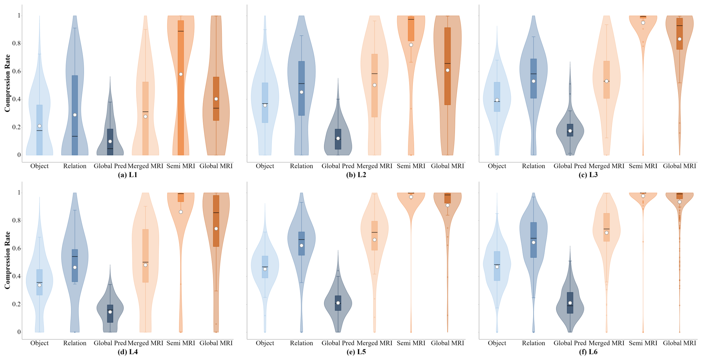
Figure 11 shows the distributions of compression rates across difficulty levels L1–L6, evaluated at the state in which the target is first derived. The six measures characterize compression at the geometric-object, relation, and global-predicate levels, together with reductions in the potential matching spaces associated with object merging, semi-conditional rules, and their combined effect.

Figure 11. Distributions of compression-related measures across FormalGeo7k difficulty levels in the solved-state setting. Each panel corresponds to one level from L1 to L6.

Across the evaluated difficulty levels, the compression-rate distributions exhibit an overall upward trend, particularly for Semi-MRI and Global MRI, whose central values approach one at L5–L6. Compression at the geometric-object and relation levels also generally increases, while global-predicate compression remains comparatively modest because it includes predicates unaffected by object merging. These observations are consistent with the expectation that more complex geometric configurations and longer reasoning chains can introduce additional equivalent object representations, redundant relations, and potential antecedent combinations, thereby providing greater opportunities for knowledge merging and semi-conditional matching. The results thus suggest that the proposed mechanisms offer greater structural compression benefits on more demanding instances.

A local reversal is observed between L3 and L4. In particular, the L4 sample exhibits lower compression than L3 on several measures, including geometric-object, relation, and global-MRI compression. This result suggests that compression depends not only on reasoning-path length but also on the geometric structures and redundancy patterns present in each subset. Since only 40 problems were sampled from each of L1–L5, the observed reversal may also reflect differences in sample composition. Evaluation on larger samples with repeated sampling within each level would help assess the stability of this pattern. Overall, the results show that compression varies across difficulty levels, with a local reversal between L3 and L4.

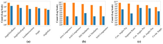
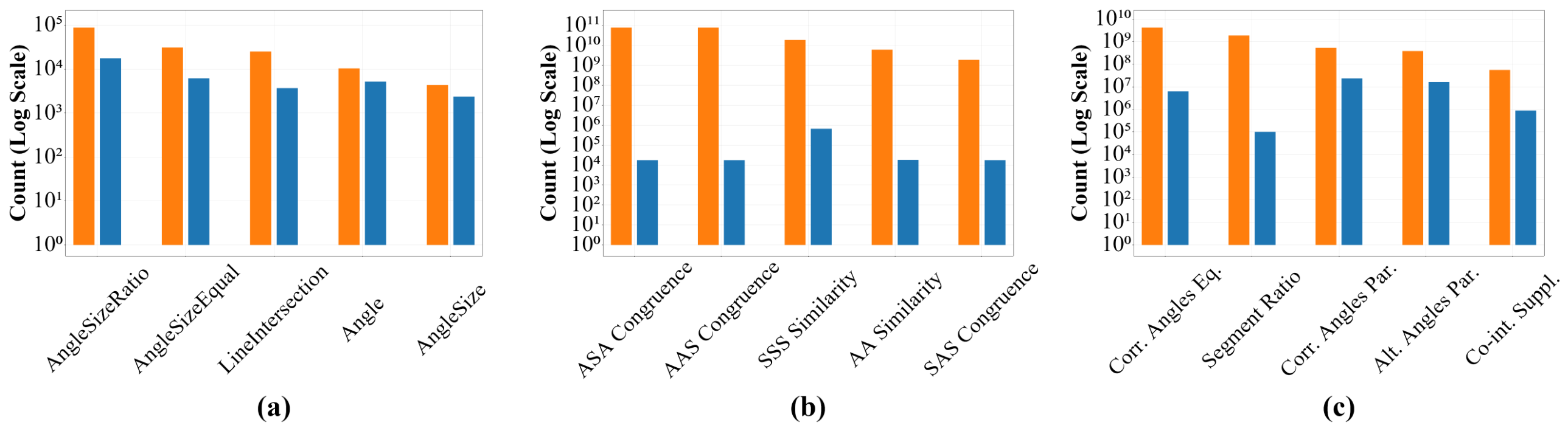
Figure 12 then compares, at the same solved state, the counts before and after compression for each mechanism, covering frequent predicates, semi-conditional rule pairs, and merged rule pairs.

Figure 12. Solved-state compression comparison on the L6 subset of FormalGeo7k. Orange and blue bars denote the counts before and after the corresponding compression operations, respectively. Panel (a) shows the counts of five predicate categories with high occurrence frequencies. Panel (b) compares the potential matching counts of semi-conditional rule pairs for different congruence and similarity criteria. Panel (c) shows the potential matching counts of rule pairs affected by geometric-object merging. All counts are measured in the knowledge state at which the target is first derived.

Figure 12a shows reductions in all five displayed predicate categories. The relative decreases are more pronounced for angle-ratio, angle-equality, and line-intersection predicates than for angle objects and angle-size predicates, indicating that compression benefits vary with the redundancy of the represented knowledge. In Figure 12b, the full-antecedent potential matching counts exceed the corresponding semi-conditional candidate counts by several orders of magnitude, with particularly large reductions for ASA and AAS congruence. This pattern is consistent with constructing candidates from base-object matches and checking the remaining instantiated constraints, thereby avoiding their participation in the full antecedent product. Figure 12c also shows substantial reductions in the potential matching counts of rules affected by object merging, with the segment-ratio category exhibiting the largest relative decrease among the displayed categories. Since antecedent counts enter the MRI multiplicatively, reductions in redundant representations can produce much larger reductions in potential rule combinations. Together, these results illustrate how compression at the knowledge-representation and rule-matching levels contributes to the overall structural reduction.

Geometric-object merging primarily reduces redundant object and relation representations and the resulting candidate space. Semi-conditional rules primarily reduce the cost of full-antecedent matching and deferred-condition verification.

5.4. Ablation Study of Chain-of-Equalities Processing

To verify the effectiveness of the chain-of-equalities matrix simplification and equation-system simplification strategies, this paper designs an ablation study that compares the full method with the variants obtained by removing the above two modules; the results are shown in Table 6. All ablation variants use the same revised implementation and rule set as the full system, with only the corresponding CE operation disabled.

Table 6. Ablation of CE processing on all 293 L6 instances. Mean and median times are calculated over each variant’s successful runs.

Variant	Solved	PSSR	Mean (s)	Median (s)
Full KM-SCR	288	98.29%	4.06	2.18
Without matrix compression	288	98.29%	9.41	3.68
Without equation simplification	273	93.17%	3.39	1.65

Removing matrix-column compression preserves the L6 success rate of 98.29%, while increasing mean solving time from 4.06 to 9.41 s and median time from 2.18 to 3.68 s. This result indicates that column compression reduces algebraic-solving overhead on this test set.

Removing equation-system simplification reduces the number of successfully solved problems from 288 to 273, indicating that this component contributes to solution coverage. Under the local strategy that processes one or two equations at a time, CE substitutions integrate variable relations distributed across multiple equalities, enabling the solution of geometric quantities that would otherwise remain unresolved. The ablated variant has a mean solving time of 3.39 s across its 273 successful runs, compared with 4.06 s across 288 successful runs for the full system. However, these means are conditioned on successful runs over different sets of problems and therefore do not establish a runtime advantage for the ablated variant. A paired comparison on the common subset of successfully solved problems is needed to isolate the runtime effect.

The two CE operations play complementary roles. Matrix-column compression reduces solving time on the tested instances without changing the number of solved problems, whereas equation-system simplification improves solving coverage under the adopted local-solving strategy.

6. Conclusions

KM-SCR integrates geometric-object merging, semi-conditional rules, and chain-of-equalities reasoning in a forward deductive system. Object merging consolidates equivalent geometric representations and their associated relations. The rule-instance equivalence proof shows that semi-conditional rules preserve the original applicability conditions and conclusion while separating candidate generation from constraint verification. Chains of equalities support direct quantitative inference and reduce the algebraic state passed to matrix and local equation solving.

The system solves 288 of the 293 FormalGeo7k-L6 problems (98.29%), with a mean solving time of 4.06 s over successful runs. The sampled L1–L5 subsets yield success rates of 97.50–100.00%. The compression analysis characterizes the reduction in represented knowledge and potential matching space, while the ablations identify complementary contributions of matrix compression to efficiency and equation simplification to solving coverage.

Future work will extend rule coverage, improve extraction of implicit problem conditions, and develop provenance tracking through matrix compression and elimination. The current workflow supports dependency-based reconstruction of recorded deductions; complete recovery of matrix-derived reasoning paths requires further work. Additional directions include three-dimensional geometry and integration with learned search guidance, where a compact symbolic state can support both inference and structured training data.

References

- Gelernter, H.; Hansen, J.R.; Loveland, D.W. Empirical explorations of the geometry theorem machine. In Proceedings of the 1960 Western Joint IRE-AIEE-ACM Computer Conference, San Francisco, CA, USA, 3–5 May 1960; pp. 143–149. [Google Scholar]
- Wu, W.T. On the decision problem and the mechanization of theorem-proving in elementary geometry. Sci. Sin. 1978, 21, 157–179. [Google Scholar]
- Buchberger, B. Bruno Buchberger’s PhD thesis 1965: An algorithm for finding the basis elements of the residue class ring of a zero-dimensional polynomial ideal. J. Symb. Comput. 2006, 41, 475–511. [Google Scholar] [CrossRef] [Scilit]
- Chou, S.C.; Gao, X.S.; Zhang, J.Z. Machine Proofs in Geometry: Automated Production of Readable Proofs for Geometry Theorems; World Scientific: Singapore, 1994. [Google Scholar]
- Chou, S.C.; Gao, X.S.; Zhang, J.Z. Automated generation of readable proofs with geometric invariants: II. Theorem proving with full-angles. J. Autom. Reason. 1996, 17, 349–370. [Google Scholar]
- Li, H. Invariant Algebras and Geometric Reasoning; World Scientific: Singapore, 2008. [Google Scholar]
- Zhang, J.Z. Outlines of point geometry. Stud. Coll. Math. 2018, 21, 1–8. (In Chinese) [Google Scholar] [CrossRef] [Scilit]
- Hu, X.L.; Jiang, J.G.; Zhang, Y. Research progress of automated particle geometry theorems proving. Adv. Appl. Math. 2018, 7, 1490–1499. (In Chinese) [Google Scholar]
- Chou, S.C.; Gao, X.S.; Zhang, J.Z. A deductive database approach to automated geometry theorem proving and discovering. J. Autom. Reason. 2000, 25, 219–246. [Google Scholar] [CrossRef] [Scilit]
- Baeta, N.; Quaresma, P. Towards a geometry deductive database prover. Ann. Math. Artif. Intell. 2023, 91, 851–863. [Google Scholar] [CrossRef] [Scilit]
- Ye, Z.; Chou, S.C.; Gao, X.S. An introduction to Java Geometry Expert. In Automated Deduction in Geometry; Sturm, T., Zengler, C., Eds.; Lecture Notes in Computer Science; Springer: Berlin/Heidelberg, Germany, 2011; Volume 6301, pp. 189–195. [Google Scholar]
- Wang, Y.; Rao, J.S.; Guan, H.; Zou, Y. NetPad: An online DGS for mathematics education. In Proceedings of the 2017 12th International Conference on Computer Science and Education (ICCSE), Houston, TX, USA, 22–25 August 2017; pp. 305–309. [Google Scholar]
- Botana, F.; Hohenwarter, M.; Janičić, P.; Kovács, Z.; Petrović, I.; Recio, T.; Weitzhofer, S. Automated theorem proving in GeoGebra: Current achievements. J. Autom. Reason. 2015, 55, 39–59. [Google Scholar] [CrossRef] [Scilit]
- Vélez, M.P. Automated reasoning for teaching and learning geometry: An open discussion. In Proceedings of the International Congress of Mathematicians 2026—Volume 7: Invited Lectures (Sections 15–20); Society for Industrial and Applied Mathematics: Philadelphia, PA, USA, 2026; pp. 566–578. [Google Scholar] [CrossRef] [Scilit]
- Rao, Y.; Xie, L.; Guan, H.; Li, J.; Zhou, Q. A method for expanding predicates and rules in automated geometry reasoning system. Mathematics 2022, 10, 1177. [Google Scholar] [CrossRef] [Scilit]
- Lu, P.; Gong, R.; Jiang, S.B.; Qiu, L.; Liang, X.D.; Zhu, S.C. Inter-GPS: Interpretable geometry problem solving with formal language and symbolic reasoning. In Proceedings of the 59th Annual Meeting of the Association for Computational Linguistics (ACL), Bangkok, Thailand, 1–6 August 2021; pp. 6774–6786. [Google Scholar]
- Wu, W.; Zhang, L.; Liu, J.; Tang, X.; Wang, Y.; Wang, S.; Wang, Q. E-GPS: Explainable geometry problem solving via top-down solver and bottom-up generator. In Proceedings of the 2024 IEEE/CVF Conference on Computer Vision and Pattern Recognition (CVPR), Seattle, WA, USA, 17–21 June 2024; pp. 13828–13837. [Google Scholar]
- Zhao, J.; Zhang, T.; Sun, J.; Tian, M.; Huang, H. Pi-GPS: Enhancing geometry problem solving by unleashing the power of diagrammatic information. In Proceedings of the 2025 IEEE/CVF International Conference on Computer Vision (ICCV), Honolulu, HI, USA, 19–23 October 2025; pp. 1526–1536. [Google Scholar]
- Zhang, X.; Zhu, N.; He, Y.; Zou, J.; Huang, Q.; Jin, X.; Guo, Y.; Mao, C.; Li, Y.; Zhu, Z.; et al. FormalGeo: An extensible formalized framework for olympiad geometric problem solving. arXiv 2023, arXiv:2310.18021. [Google Scholar]
- He, Y.; Zou, J.; Zhang, X.; Zhu, N.; Leng, T. FGeo-TP: A language model-enhanced solver for Euclidean geometry problems. Symmetry 2024, 16, 421. [Google Scholar] [CrossRef] [Scilit]
- Zhang, X.; Li, Y.; Zhu, N.; Qin, C.; Zeng, Z.; Leng, T. FGeo-HyperGNet: Geometric problem solving integrating FormalGeo symbolic system and hypergraph neural network. In Proceedings of the Thirty-Fourth International Joint Conference on Artificial Intelligence (IJCAI), Montreal, QC, Canada, 16–22 August 2025; pp. 4733–4741. [Google Scholar]
- Li, Y.; Zhang, X.; Qin, C.; Hu, Z.; Leng, T. FGeo-ISRL: A MCTS-enhanced deep reinforcement learning system for plane geometry problem-solving via inverse search. Symmetry 2026, 18, 628. [Google Scholar] [CrossRef] [Scilit]
- Hu, Z.; Zhang, X.; Qin, C.; Li, Y.; Leng, T. A hybrid framework for automated geometric problem-solving by integrating formal symbolic systems and deep learning. Symmetry 2026, 18, 592. [Google Scholar] [CrossRef] [Scilit]
- Zhang, C.; Song, J.; Li, S.; Liang, Y.; Ma, Y.; Wang, W.; Zhu, Y.; Zhu, S.-C. Proposing and solving olympiad geometry with guided tree search. Nat. Mach. Intell. 2026, 8, 84–95. [Google Scholar] [CrossRef] [Scilit]
- Trinh, T.H.; Wu, Y.; Le, Q.V.; He, H.; Luong, T. Solving olympiad geometry without human demonstrations. Nature 2024, 625, 476–482, Correction in Nature 2024, 627, E8. https://doi.org/10.1038/s41586-024-07115-7. [Google Scholar] [CrossRef] [Scilit]
- Chervonyi, Y.; Trinh, T.H.; Olšák, M.; Yang, X.; Nguyen, H.H.; Menegali, M.; Jung, J.; Kim, J.; Verma, V.; Le, Q.V.; et al. Gold-medalist performance in solving olympiad geometry with AlphaGeometry2. J. Mach. Learn. Res. 2025, 26, 1–39. [Google Scholar]
- Nevins, A.J. A relaxation approach to splitting in an automatic theorem prover. Artif. Intell. 1975, 6, 25–39. [Google Scholar] [CrossRef] [Scilit]
- Duan, B.; Liang, X.; Lu, S.; Wang, Y.; Shen, Y.; Chang, K.-W.; Wu, Y.N.; Yang, M.; Chen, W.; Gong, Y. Gold-medal-level olympiad geometry solving with efficient heuristic auxiliary constructions. In Proceedings of the 64th Annual Meeting of the Association for Computational Linguistics (Volume 1: Long Papers); Association for Computational Linguistics: San Diego, CA, USA, 2026; pp. 21725–21747. [Google Scholar]
- Olšák, M.; Kaliszyk, C.; Urban, J. Property invariant embedding for automated reasoning. In Proceedings of the ECAI 2020: 24th European Conference on Artificial Intelligence, Santiago de Compostela, Spain, 29 August–8 September 2020; pp. 1395–1402. [Google Scholar]
- Wang, D. GEOTHER 1.1: Handling and proving geometric theorems automatically. In Automated Deduction in Geometry (ADG 2002); Winkler, F., Ed.; Lecture Notes in Computer Science; Springer: Berlin/Heidelberg, Germany, 2004; Volume 2930, pp. 194–215. [Google Scholar]
- Wang, K.; Su, Z.D. Automated geometry theorem proving for human-readable proofs. In Proceedings of the Twenty-Fourth International Joint Conference on Artificial Intelligence (IJCAI), Buenos Aires, Argentina, 20–31 July 2015; pp. 3133–3139. [Google Scholar]
- Liu, D.; Gu, T.; Xue, J.P. Rule engine based on improvement rete algorithm. In Proceedings of the 2010 International Conference on Apperceiving Computing and Intelligence Analysis (ICACIA), Chengdu, China, 17–19 December 2010; pp. 346–349. [Google Scholar]
- Zhang, X.; Zhu, N.; Qin, C.; Li, Y.; Zeng, Z.; Leng, T. Formal representation and solution of plane geometric problems. In Proceedings of the NeurIPS 2024 Workshop on Mathematical Reasoning and AI (MATH-AI), Vancouver, BC, Canada, 14 December 2024. [Google Scholar]
- Gan, W.; Yu, X.; Zhang, T.; Wang, M. Automatically proving plane geometry theorems stated by text and diagram. Int. J. Pattern Recognit. Artif. Intell. 2019, 33, 1940003. [Google Scholar] [CrossRef] [Scilit]
- Huang, Q.; Zhang, X.; Zhu, N.; Zhu, F.; Leng, T. FGeo-eval: Evaluation system for plane geometry problem solving. Symmetry 2025, 17, 902. [Google Scholar] [CrossRef] [Scilit]
- Zhang, X.; Zhu, N.; He, Y.; Zou, J.; Qin, C.; Li, Y.; Leng, T. FGeo-SSS: A search-based symbolic solver for human-like automated geometric reasoning. Symmetry 2024, 16, 404. [Google Scholar] [CrossRef] [Scilit]
- Zou, J.; Zhang, X.; He, Y.; Zhu, N.; Leng, T. FGeo-DRL: Deductive reasoning for geometric problems through deep reinforcement learning. Symmetry 2024, 16, 437. [Google Scholar] [CrossRef] [Scilit]
Disclaimer/Publisher’s Note: The statements, opinions and data contained in all publications are solely those of the individual author(s) and contributor(s) and not of MDPI and/or the editor(s). MDPI and/or the editor(s) disclaim responsibility for any injury to people or property resulting from any ideas, methods, instructions or products referred to in the content. |
© 2026 by the authors. Licensee MDPI, Basel, Switzerland. This article is an open access article distributed under the terms and conditions of the Creative Commons Attribution (CC BY) license.