


Abstract
Quantitative trajectory analysis commonly summarizes biological motion using global geometric or dynamical descriptors, but these do not directly quantify how movement statistics vary across space or time. Here, we present BioTraj, an open-source Python framework integrating video-based trajectory extraction, conventional movement descriptors, and information-geometric analysis. Local and time-resolved turning angle distributions are represented on the probability simplex and compared using the Fisher–Rao geodesic distance. Spatial and temporal Fisher–Rao measures thereby quantify distributional heterogeneity without predefined behavioral states. The method is validated using simulated trajectories with a deliberately imposed stationary, spatial, temporal, and spatiotemporal structure, while sampling controls characterize finite-sample sensitivity. The workflow is then applied to ant recordings using independently defined scene annotations. In the Yellow ant recording, Fisher–Rao heterogeneity differed broadly inside and outside the historical footprint of a removed rock after controlling for tracking domain edges, whereas small candidate nest openings were unresolved at the selected grid scale. In the Wall recording, annotated surfaces exhibited different local heterogeneity, while distance from surface transitions showed no universal monotonic response. BioTraj therefore provides a descriptive, reproducible framework for identifying where movement statistics change and relating these changes to an independently annotated environmental context, rather than automatically assigning behavioral states.
Keywords:
information geometry; Fisher–Rao distance; biological trajectories; movement analysis; turning angles; computer vision; Python; OpenCV MSC:
62B11; 92B05
1. Introduction
Quantitative analysis of movement trajectories is central to movement ecology, behavioral biology, microbiology, biophysics, and active matter research. A trajectory contains information about spatial exploration, directional persistence, transport, confinement, and interactions with the surrounding environment [1,2,3,4]. Improvements in digital imaging and computer vision now make it possible to obtain large trajectory datasets using inexpensive cameras and open-source software [5,6,7].
Once trajectories have been reconstructed, however, their quantitative interpretation remains non-trivial. Global descriptors such as the explored area, anisotropy, mean-squared displacement, straightness, and fractal dimension summarize important aspects of motion but compress heterogeneous trajectories into a small number of quantities. Occupancy maps retain spatial information but primarily describe where observations occur rather than whether the statistical character of movement changes between different parts of the explored domain. Movement ecology methods based on random walks, state-space models, and hidden Markov models provide powerful alternatives, frequently modeling step lengths and turning angles as state-dependent distributions [8,9]. Such approaches are especially useful when the objective is inference about a finite set of latent behavioral states. In other situations, it may instead be useful to quantify spatial or temporal changes in empirical movement distributions directly, without first assigning observations to discrete behavioral states.
For example, an organism may move similarly over most of a recording but alter its turning behavior after crossing from one surface to another, or only during a restricted time interval. A single value calculated over the complete trajectory can average over such localized changes. The aim here is therefore not only to summarize a trajectory globally, but also to identify where and when its empirical movement statistics differ.
Information geometry provides a natural mathematical framework for this problem. Probability distributions can be regarded as points on a statistical manifold equipped with the Fisher information metric, with geodesic distance providing an intrinsic measure of separation between statistical states [10,11]. For discrete probability distributions, the square root embedding maps the probability simplex, equipped with the Fisher–Rao metric, isometrically to the positive orthant of a hypersphere, yielding a simple closed-form expression for the Fisher–Rao geodesic distance [12]. This construction is particularly convenient for normalized empirical histograms derived from trajectory data.
Here, we introduce this approach into BioTraj, an open-source Python framework for video tracking and quantitative trajectory analysis. In addition to conventional descriptors, BioTraj constructs local and time-resolved turning angle distributions and compares them using Fisher–Rao geodesic distances. The resulting spatial information gradient maps and temporal distance matrices characterize how movement statistics vary across the explored domain and through time. The analysis identifies regions or periods with statistically different movement distributions without automatically assigning biological labels such as “foraging” or “searching”. Trajectory identifiers are therefore treated as continuous track segments rather than assumed individual identities.
The information-geometric analysis is validated using simulated trajectories with a known imposed statistical structure, including stationary, spatial, temporal, and combined spatiotemporal cases. These benchmarks test whether imposed spatial and temporal changes are recovered and quantify the influence of finite local sample size on empirical Fisher–Rao distances. Selected ant population recordings are then analyzed as independent real-data demonstrations of the workflow. Because these recordings are non-systematic field observations rather than controlled experiments, they are used to demonstrate annotation-aware interpretation of information-geometric maps rather than to infer causal environmental effects or rank behavioral differences among recordings.
BioTraj therefore connects conventional trajectory analysis with an information-geometric description of local and time-resolved movement distributions. It provides a reproducible workflow from video-derived trajectories to spatial and temporal maps of distributional heterogeneity while retaining conventional trajectory descriptors as complementary measures.
The principal scientific and practical contributions of the present work are therefore threefold: (i) an open-source workflow combining video-derived trajectories with conventional movement descriptors; (ii) a state-free information-geometric analysis for mapping spatial and temporal changes in empirical movement distributions without requiring a predefined number of behavioral states; and (iii) a validation framework that examines synthetic ground-truth recovery, finite-sampling effects, parameter sensitivity, alternative distributional measures, and robustness to plausible trajectory imperfections before interpretation of experimental recordings.
2. Materials and Methods
2.1. The BioTraj Framework
BioTraj (version 1.2) is an open-source Python (version 3.13.12) framework in which trajectory extraction and quantitative analysis are implemented as separate modules. The tracking module uses OpenCV [6,7] for image processing, object detection, and centroid-based trajectory reconstruction, and exports the resulting coordinates for subsequent analysis. The analysis module computes conventional trajectory descriptors together with the spatial and temporal information-geometric measures investigated in this study. This separation allows the analysis to be applied to compatible trajectory coordinates produced by BioTraj or by other tracking workflows.
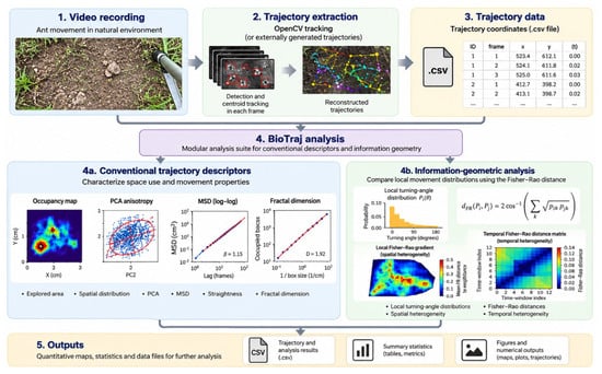
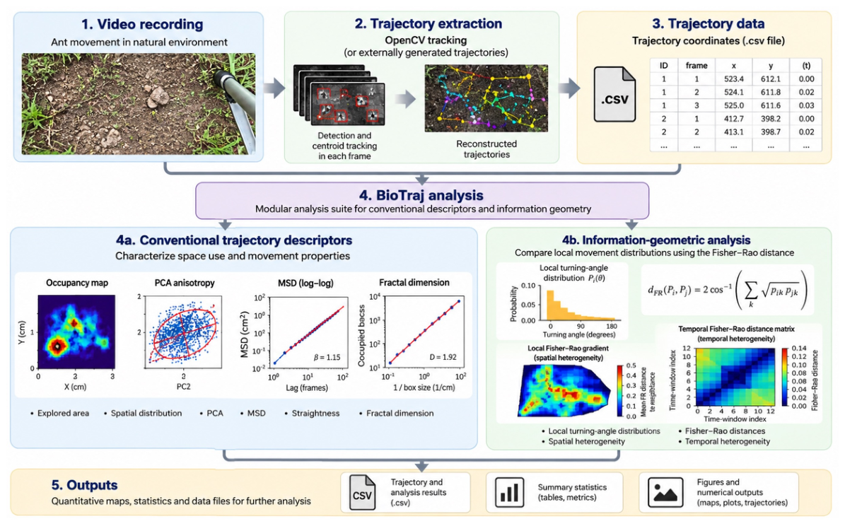
Figure 1 summarizes the analysis workflow used in this study. Video-derived trajectories may be obtained using the OpenCV-based tracking module or imported from other compatible tracking workflows. The resulting trajectory coordinates are analyzed using conventional movement descriptors and the spatial and temporal information-geometric analyses developed here.
Figure 1.
Overview of the BioTraj analysis workflow. Video recordings are processed to extract trajectories using OpenCV-based tracking or compatible trajectory coordinates may be supplied by external tracking workflows. The resulting trajectory data are analyzed using conventional descriptors of spatial exploration and movement together with information-geometric analysis based on local turning angle distributions and Fisher–Rao distances. The latter provides spatial and temporal measures of distributional heterogeneity. The workflow produces quantitative maps, summary statistics, and numerical data outputs. Example plots within the workflow are schematic representations of the corresponding analysis outputs rather than additional experimental results.
The biological recordings used for the experimental demonstrations were acquired using iPhone 8 and iPhone X smartphones (Apple Inc., Cupertino, CA, USA) at a resolution of 1920 × 1080 pixels. Trajectories generated by other tracking software can also be imported directly into the analysis module.
2.1.1. Relationship to Existing Trajectory Analysis Tools
A range of established open-source tools is available for extracting biological trajectories from image sequences, including TrackMate [13], ToxTrac [14], DeepLabCut [15], and idtracker.ai [16]. These packages address different tracking problems, including particle and cell tracking, automated animal tracking, markerless pose estimation, and identity-preserving multi-animal tracking. BioTraj does not seek to reproduce or benchmark these capabilities.
The purpose of the present framework is instead to provide a reproducible implementation of the trajectory analysis workflow investigated in this study, with particular emphasis on spatially and temporally resolved comparison of empirical movement distributions using Fisher–Rao geometry. The analysis module operates on exported trajectory coordinates and can therefore also be applied to trajectories obtained using other tracking methods. Conventional descriptors are included as complementary measures that provide context for the information-geometric analysis.
The present analysis is also complementary to statistical trajectory segmentation and change detection approaches. State-space and hidden Markov models are designed to infer latent states under an explicit probabilistic model, whereas nonparametric distributional comparisons can ask whether two empirical samples differ without assigning them to predefined states. BioTraj adopts the latter perspective locally in space and through time using the Fisher–Rao geometry of empirical movement distributions. Its advantage is therefore a state-free and spatially explicit representation of distributional heterogeneity. Its corresponding limitations include finite-sample dependence and sensitivity to the chosen histogram, spatial, and temporal resolutions. These approaches address related but not identical questions and should be regarded as complementary rather than interchangeable.
Table 1 places this role alongside representative open-source trajectory tools. The comparison is intentionally based on the principal purpose of each package rather than on an exhaustive feature-by-feature benchmark. In particular, the packages listed below provide sophisticated solutions to tracking, identity preservation, or pose estimation, whereas the present contribution focuses on downstream, state-free comparison of empirical movement distributions in space and time. The approaches are therefore largely complementary: BioTraj can analyze compatible coordinates produced by external tracking workflows rather than requiring its own tracker.
Table 1.
Representative comparison between BioTraj and established open-source tools used in biological trajectory workflows. The comparison emphasizes their principal objectives and the aspects most relevant to the present study; it is not intended as an exhaustive software benchmark. The comparison summarizes the cited literature rather than version-specific performance tests.
The methodological distinction summarized in Table 1 is that BioTraj treats turning angle samples from spatial cells or temporal windows as empirical probability distributions, rather than reducing each sample to a single movement descriptor. Fisher–Rao geodesic distances then quantify differences between these distributions on the probability simplex. Spatial neighbor comparisons and consecutive temporal window comparisons provide complementary maps of distributional heterogeneity. This is a state-free, descriptive approach; it does not infer behavioral states or establish the biological causes of a detected change. The contribution is therefore the integrated spatially and temporally resolved application of established information geometry to trajectory analysis, not a new Fisher–Rao metric.
2.1.2. Software Availability
BioTraj is implemented in Python and distributed as open-source software through a public GitHub repository under the MIT License. The repository contains the complete source code, installation instructions, example videos and trajectory datasets, configuration files, and documentation required to reproduce and test the analysis workflow. The analyses reported here were performed using BioTraj version 1.2.
BioTraj requires Python 3.10 or later. The analyses reported here used Python 3.13.12, OpenCV 4.11.0, NumPy 2.3.2, SciPy 1.16.1, Matplotlib 3.10.6, and pandas 2.2.3. It accepts video recordings for trajectory extraction and compatible CSV trajectory files for independent analysis, and produces numerical summaries, processed data files, and graphical summaries. The tracking and analysis components are separated through exported trajectory files, allowing the analysis modules to be applied independently and facilitating the addition of new analysis methods without modification of the tracking component.
2.2. Trajectory Analysis Methods
The quantitative analysis of trajectories is an important topic in statistical physics, where particle motion is often characterized through geometric and dynamical descriptors. Similar approaches can be applied to biological trajectories, allowing concepts originally developed for diffusion, random walks, and transport processes to be explored using real experimental data. A biological trajectory may be represented as a sequence of positions , sampled at discrete times . From these positions, a variety of statistical descriptors can be computed to characterize spatial exploration, directional organization, and transport properties.
2.2.1. Explored Area
The spatial extent explored by the trajectories is characterized using the convex hull of the recorded positions, defined as the smallest convex polygon containing the trajectory dataset. Its area provides a simple global descriptor of the region sampled during a recording. A Monte Carlo estimate of the enclosed area is additionally calculated as a numerical consistency check by sampling random points within the corresponding bounding rectangle. Explored area measurements are used here as conventional descriptive quantities and are not part of the information-geometric analysis.
2.2.2. Occupancy Maps
While the explored area indicates the spatial extent of motion, it does not reveal how frequently different regions are visited. Occupancy maps are therefore constructed by dividing the explored region into spatial bins and counting the number of trajectory positions falling within each bin. Occupancy maps provide a visual representation of space utilization and can reveal preferred pathways, highly visited regions, and areas that are rarely explored.
2.2.3. Principal Component Analysis and Anisotropy
Spatial anisotropy is characterized by principal component analysis (PCA) of the trajectory coordinates [17]. If are the eigenvalues of the coordinate covariance matrix, the anisotropy ratio is defined as follows:
Values near unity indicate approximately isotropic exploration, whereas larger values indicate increasingly elongated spatial distributions.
2.2.4. Mean-Squared Displacement
Transport behavior is characterized using the mean-squared displacement (MSD) [3]:
where is the time lag. Approximate power-law behavior is summarized as . Values near correspond to normal diffusion, whereas indicates superdiffusive motion [4,18].
2.2.5. Straightness Index
Trajectory geometry can be quantified using the straightness index:
The straightness index compares the net displacement with the total path length. Values close to unity indicate nearly straight trajectories, whereas smaller values correspond to increasingly tortuous paths.
2.2.6. Fractal Dimension
Trajectory complexity is additionally characterized using the box-counting fractal dimension:
where is the number of boxes of size intersecting the trajectory [19,20]. In the present study, fractal dimension is retained as a conventional complementary descriptor. Values for the experimental recordings are reported in the Supporting Information.
2.2.7. Information-Geometric Analysis of Local Movement Distributions
The conventional descriptors above summarize complementary geometric and dynamical properties, but they do not directly measure changes in the full local distribution of a movement variable. BioTraj therefore includes an information-geometric module based on turning angles. Turning angle was selected for the present implementation because it is invariant to rotation of the camera coordinate system and can be calculated within track segments without requiring absolute orientation.
Turning Angle Distributions
Observations are grouped by track identifier and ordered by frame number. Track identifiers are treated as trajectory segments for analysis and are not assumed to correspond uniquely to biological individuals. For three successive stored positions belonging to the same track segment, displacement vectors are defined by
The unsigned turning angle is
with . A turning angle observation is discarded when either displacement has zero length or when the middle coordinate is non-finite. The angle is associated with the middle position of the corresponding three-point sequence. The production implementation does not additionally require the three observations to occur in consecutive video frames; consequently, if a tracker retains the same identifier across a short detection gap, an angle may span that gap.
The present implementation uses unsigned turning angles and therefore characterizes the magnitude of directional reorientation rather than left–right turning handedness. Consequently, trajectories that differ only in preferential clockwise versus anticlockwise turning are not distinguished by this representation. This is a deliberate simplification of the present implementation and is considered further among the methodological limitations.
For a spatial cell or temporal window a, the observed turning angles are converted to a normalized histogram
All analyses reported here used equal-width bins over the interval 0–, corresponding to a bin width of . No pseudocount was used (i.e., no artificial counts were added to histogram bins). Spatial cells containing fewer than 30 valid turning angle observations and temporal windows containing fewer than 100 observations were excluded from the corresponding information-geometric comparisons.
The Square Root Embedding
The square root embedding
maps the probability simplex isometrically under the Fisher metric convention used here to the positive orthant of a sphere of radius 2 because . Equivalently, the unscaled square root vector lies on the unit sphere. For two empirical distributions P and Q, BioTraj uses the Fisher–Rao geodesic distance
where the factor of two specifies the metric convention used throughout this work. Equation (9) gives the Fisher–Rao geodesic distance between categorical distributions under the metric convention adopted here [10,11,12].
Spatial Information Geometry
The analyzed image domain is partitioned into spatial cells . Each turning angle is assigned to the regular grid cell containing its middle position . For each sufficiently sampled cell, BioTraj estimates a normalized turning angle distribution and evaluates Fisher–Rao distances . The complete matrix D describes statistical similarity independently of physical separation.
Local information-geometric heterogeneity is summarized by the local Fisher–Rao gradient
where contains the valid orthogonally adjacent cells (north, south, east, and west) only. Diagonal neighbors are not used. At image or ROI boundaries, or next to undersampled cells, only available valid neighbors contribute to the mean. If a valid cell has no valid orthogonal neighbor, is left undefined rather than assigned a numerical zero. The term “gradient” therefore denotes a discrete local contrast in probability distribution space rather than a differential spatial derivative.
Large values of identify regions across which local turning angle distributions differ strongly, whereas small values indicate locally similar movement statistics. This map is complementary to an occupancy map: occupancy measures spatial use, whereas the Fisher–Rao field measures variation in the statistical character of movement.
Temporal Information Geometry
For temporal analysis, the recording is divided into windows . A turning angle distribution is estimated for each sufficiently sampled window, producing a temporal Fisher–Rao matrix . Consecutive window distances
provide a direct measure of distributional change through time. In the present analyses, 15 s non-overlapping windows were used for recordings acquired at 60 frames . Thus, each temporal window and step comprised 900 frames. The temporal resolution therefore limits localization of an abrupt transition: a transition occurring inside a window produces a mixed distribution in that window and may generate the largest consecutive distance at the following fully post-transition window.
Sampling and Uncertainty
Empirical histogram distances depend on the number of observations available to estimate each distribution. Cells or windows below the minimum numbers specified above are therefore excluded. Bootstrap uncertainty for a Fisher–Rao comparison is obtained by independently resampling the two underlying turning angle samples with replacement, retaining the original sample size of each sample. A histogram and Fisher–Rao distance are recomputed for each bootstrap replicate. The implementation reports the bootstrap standard deviation and the 2.5th and 97.5th percentiles; the latter define the displayed 95% percentile interval. For a local gradient, neighbor-specific percentile limits are averaged over the same valid orthogonal neighbors used to compute . The reference spatial and temporal analyses used 200 bootstrap replicates.
Additional threshold convergence and equal-sample analyses were used to diagnose finite-sampling effects. The equal-count finite-sampling control drew 100 turning angles from each eligible spatial cell and repeated the calculation 200 times. The Supplementary Materials additionally report threshold convergence curves and the number of spatial cells retained as the minimum-count criterion is increased. These controls are important when spatial sampling is strongly heterogeneous. The current bootstrap treatment quantifies empirical sampling variability but does not make independent individual assumptions; temporally correlated observations and fragmented tracklets remain considerations for inferential applications.
2.2.8. Independent Scene Annotation and Annotation-Aware Analysis
To relate information-geometric structure to visible features of the recording environment without defining regions from the Fisher–Rao result itself, BioTraj supports independent scene annotations in the original image coordinate system. Annotations are stored separately from the trajectory data and may represent polygonal surfaces or biological regions, polylines marking physical or surface transitions, circular features, observation boundaries, or artifact regions. This distinction separates the tracking domain from biologically or physically meaningful regions and from optional quality control masks.
For an annotated polygonal surface S, each valid information-geometric cell is assigned according to the position of its cell center. For an annotated transition represented by a polyline , the distance of cell i with center is
For the Yellow ant analysis, the former rock footprint is represented by an independently annotated polygon . A signed distance to its boundary is calculated from each cell center as
where is the minimum Euclidean distance from the cell center to the polygon boundary. Thus, negative values denote cells inside the former rock footprint and positive values denote cells outside it. This signed distance calculation was used for the Yellow ant boundary analysis described below.This permits descriptive comparison of the local Fisher–Rao gradient among independently defined regions and as a function of distance from physical transitions. Annotations designated as artifacts can additionally be used to generate quality-controlled summaries while preserving the unmasked result. Scene annotations used for interpretation were defined from the video frame independently of the Fisher–Rao map.
The annotation-aware analysis is intentionally descriptive. Spatial cells are not treated as independent biological replicates, and no inferential p-values are calculated from cell-level differences. Region summaries therefore report cell counts and distributional statistics, while mechanistic interpretation requires independent biological or physical evidence.
3. Results
3.1. Method Validation and Experimental Demonstration
Simulated trajectories were used to test whether the information-geometric analysis recovered deliberately imposed spatial and temporal changes in movement statistics. Each simulation contained 20 agents propagated for more than 12,000 frames, yielding more than 240,000 recorded positions. This simulation length was chosen to generate trajectory datasets comparable in scale to the experimental recordings analyzed subsequently while providing sufficient observations for repeated spatial and temporal estimation.
Four simulation scenarios were generated using the same random seed and analysis settings: a stationary control, a spatial transition at pixels (between pixel columns 952 and 953), a temporal transition at frame 6058 ( s at 60 frames ), and a combined spatiotemporal case. The simulated movement model updates direction using a von Mises turning distribution and draws positive step lengths from a truncated normal distribution. It is intended as a controlled validation model rather than a mechanistic model of ant behavior. The four reference scenarios used 20 agents, 12,116 frames (242,320 recorded positions), a pixel arena, 60 frames . A common seed was deliberately used in the originally submitted benchmark so that differences among the four scenarios reflected the imposed statistical structure rather than unrelated stochastic realizations. Spatial analyses used a grid with at least 30 turning angle observations per cell, whereas temporal analyses used non-overlapping 15 s windows with at least 100 observations per window. The spatial histograms used 18 angular bins, no pseudocount, and 200 bootstrap replicates. Temporal analyses likewise used 200 bootstrap replicates.
For independent replication, Table S2 in the Supplementary Materials reports the reference analysis settings, while Table S3 documents the stochastic generator, the distribution parameters defining each scenario before and after the imposed changes, and the random seed protocol for the 20-replicate validation.
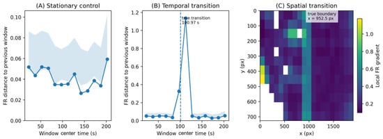
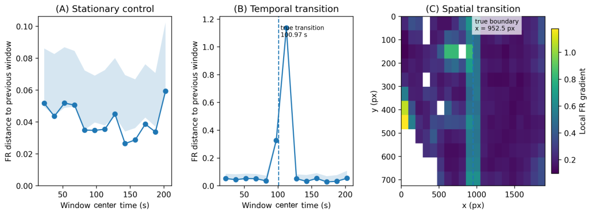
Figure 2 summarizes the simulation-based validation. The stationary simulation produced only small consecutive temporal Fisher–Rao distances (maximum ). In the simulation containing a temporal transition, the 90–105 s window containing the imposed change showed an increased response (), while the largest consecutive distance occurred in the following comparison involving the fully post-transition distribution (, bootstrap interval approximately 1.114–1.162). The combined spatiotemporal simulation also produced a pronounced temporal response (maximum , approximately 0.805–0.846).
Figure 2.
Validation of the BioTraj information-geometric analysis using simulated trajectories. (A) Stationary control showing the Fisher–Rao distance between successive temporal windows when the underlying movement distribution is unchanged. (B) Temporal two-state benchmark. The imposed transition at s (dashed line) produces a marked information-geometric response within the temporal resolution of the 15 s analysis windows. (C) Spatial two-domain benchmark. The imposed boundary at px (dashed line) coincides with the region of increased local Fisher–Rao gradient. Together, these simulations demonstrate recovery of deliberately imposed temporal and spatial changes within the resolution of the analysis.
For the spatial transition simulation, the imposed boundary lay between grid columns 9 and 10 and was recovered as increased local Fisher–Rao heterogeneity around these columns. The simulations therefore demonstrate that the analysis distinguishes stationary from changing movement distributions and localizes imposed changes within the spatial and temporal resolution defined by the analysis grid and window length.
The stochastic validation was then repeated over 20 independent random seeds for each of the four scenarios. Across 260 consecutive window comparisons from the stationary null simulations, the mean Fisher–Rao distance was 0.044 (SD 0.008), with a 95th percentile of 0.057 and a maximum of 0.078. In contrast, the temporal transition and combined spatiotemporal scenarios produced mean peak distances of and , respectively, and the transition-spanning comparison was recovered in 20/20 realizations in both cases.
Sensitivity analyses additionally varied spatial grid resolution, turning angle histogram resolution, minimum spatial sampling threshold, and temporal window length. Absolute Fisher–Rao values changed with analysis resolution, as expected for empirical histogram estimates, but the imposed temporal transition was recovered in all 360 transition-containing analyses across the tested parameter configurations and seeds. A separate change magnitude analysis showed a monotonic increase in the Fisher–Rao response as the imposed difference between the two turning angle distributions increased.
Finally, the temporal benchmarks were repeated using Hellinger, Jensen–Shannon, and linear and circular Wasserstein distances, together with the absolute change in mean turning angle as a conventional scalar reference. All measures recovered the strong imposed transition in this controlled benchmark. These comparisons are not interpreted as demonstrating universal superiority of the Fisher–Rao distance; rather, the Fisher–Rao distance is retained because it provides the intrinsic geodesic associated with the statistical geometry adopted here. Complete numerical results and parameter settings are reported in the Supplementary Materials.
3.1.1. Finite-Sampling Robustness
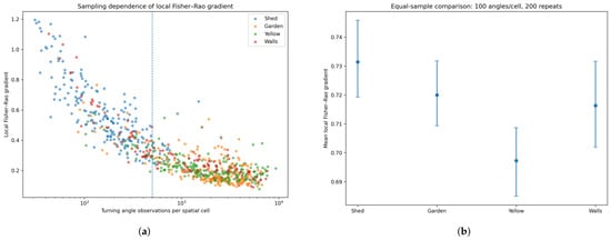
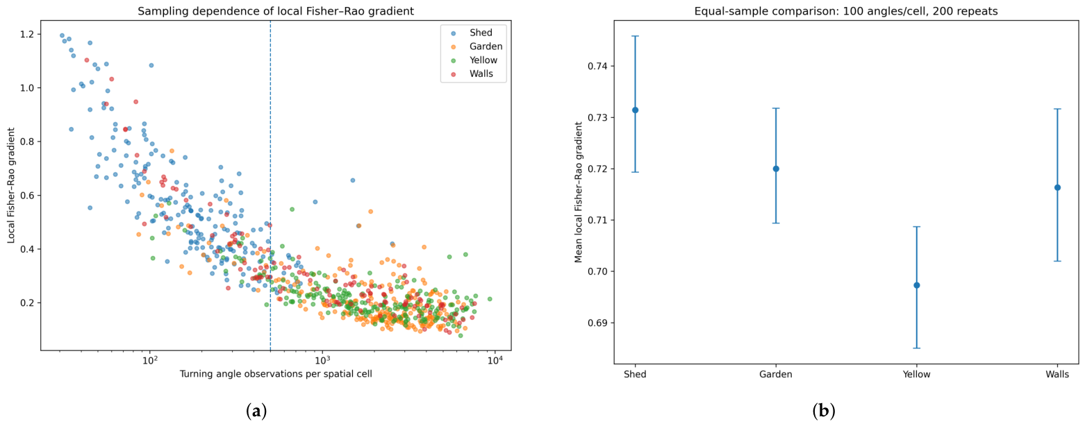
Figure 3 summarizes the finite-sampling diagnostics. Empirical Fisher–Rao distances depend on the number of observations used to estimate each histogram. Across the experimental recordings, sparsely sampled cells tended to have larger raw local gradients. Increasing the minimum cell count and performing equal-count resampling confirmed that a substantial component of raw between-cell and between-recording variation can arise from finite-sample estimation noise. When 100 turning angles were drawn from each eligible cell and the calculation repeated 200 times, the four recordings converged to similar mean local gradients (approximately 0.70–0.73). These equal-sample values are therefore treated as a diagnostic of sampling sensitivity rather than as biological effect sizes.
Figure 3.
Finite-sampling behavior of the empirical local Fisher–Rao gradient. (a) Local Fisher–Rao gradient as a function of the number of turning angle observations available in each spatial cell for the four experimental recordings. Larger and more variable gradients occur in sparsely sampled cells, demonstrating a finite-sampling contribution to the empirical Fisher–Rao distance. (b) Equal-sample control obtained by restricting each cell to 100 turning angle observations and repeating the sampling 200 times. The plotted central values are the means across the 200 equal-sample resampling repetitions, and the error bars indicate the 2.5th–97.5th percentile interval across those repetitions. Standardizing the sampling level substantially reduces the apparent between-dataset differences, illustrating the importance of controlling sample size when comparing empirical Fisher–Rao gradients across recordings.
The practical consequence is that local Fisher–Rao maps are interpreted together with minimum-count filtering and sampling diagnostics, and raw mean gradients are not used to rank independent recordings. The Supplementary Materials explicitly examine sensitivity to the minimum spatial sampling threshold by plotting both local Fisher–Rao heterogeneity and the number of retained cells as the threshold is increased. They also report dataset-specific relationships between local sample count and gradient and the complete equal sampling distributions. These diagnostics are retained as Supplementary Materials because they validate finite-sampling robustness but are not used as biological effect sizes.
3.1.2. Experimental Demonstration with Independent Scene Annotations
Following simulation-based validation, BioTraj was applied to ant recordings as demonstrations on realistic biological data. The recordings were not designed as controlled environmental treatments and are not treated as biological replicates. The ants in the Meadow, Shed, and Wall recordings had a broadly similar dark appearance, consistent with common black garden ants of the Lasius niger group, whereas the distinctly pale-yellow ants recorded beneath a concrete rock were consistent in appearance and habitat with the yellow meadow ant, Lasius flavus. These associations are based on gross appearance and habitat rather than formal taxonomic identification, as specimens were not collected for species-level determination. Accurate species-level identification was not required for the purpose of the present study, which used the recordings to demonstrate the analysis of spatial and temporal heterogeneity in movement distributions rather than to compare species-specific behavior. The descriptive recording labels are therefore retained throughout the analysis. Two recordings are emphasized because they test complementary uses of independent scene annotation: a biologically contextual region in the Yellow ant recording and macroscopic physical surfaces in the Wall recording.
Yellow Ants: Historical Rock Footprint and Candidate Nest Openings
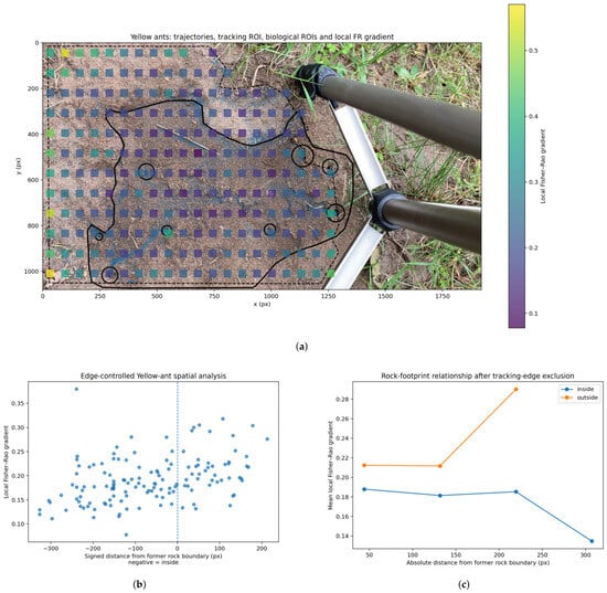
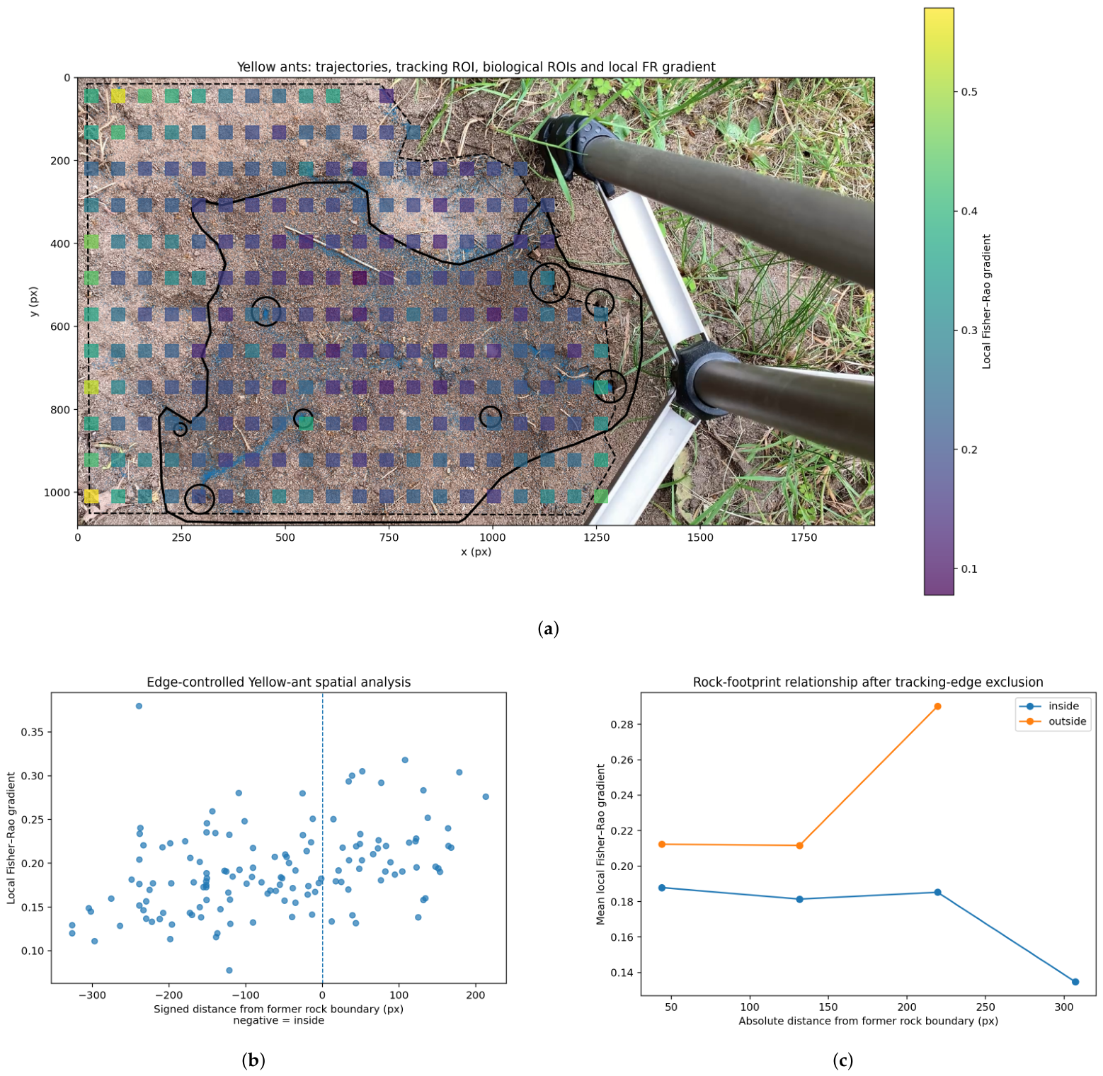
The Yellow ant recording was obtained after a large rock covering the observed area had been lifted. The former rock footprint and eight candidate nest openings were annotated from the scene independently of the Fisher–Rao map. Because cells close to the tracking domain boundary showed elevated local gradients, an edge-controlled analysis excluded cells within one grid cell width (approximately 88 pixels) of that boundary before regional interpretation.
After edge control, 139 cells were retained. Cells inside the former rock footprint had a mean local Fisher–Rao gradient of 0.181 (median 0.177; ), compared with 0.215 (median 0.214; ) outside, corresponding to an outside–inside ratio of approximately 1.19. In contrast, cells near the candidate nest openings showed only a small difference from cells farther from the openings (mean 0.204 versus 0.196 in the edge-controlled analysis). The openings were smaller than the spatial cells used for information geometry, so the analysis does not support localization of individual entrances at this resolution. The result is therefore interpreted as a broad regional association with the historical rock-covered area rather than as detection of individual nest openings or a causal habitat effect.
Additional within-recording robustness tests were performed on the Yellow ant trajectories. Requiring strict frame-to-frame continuity removed 20.51% of turning angles accepted by the production calculation but strongly preserved the spatial organization of the gradient map ( across paired cells) and retained the direction of the annotated outside–inside contrast. Controlled Gaussian coordinate perturbations with , 1.0, and 2.0 pixels likewise retained a positive regional contrast in all 60 realizations, while map agreement decreased progressively with increasing perturbation as expected. Spatial block bootstrap analyses using contiguous and cell blocks also retained positive within-recording contrast intervals. These calculations assess computational robustness within this recording and are not confidence intervals across independent colonies or biological replicates. Full results are provided in the Supporting Information.
Figure 4 presents the annotation-aware Yellow ant analysis.
Figure 4.
Annotation-aware analysis of the Yellow ant recording.(a) Local Fisher–Rao gradient superimposed on the recording scene together with the independently annotated former rock footprint and candidate nest openings. (b) Local Fisher–Rao gradient as a function of signed distance from the former rock boundary after exclusion of cells close to the tracking domain edge. Negative distances denote locations inside the former footprint. (c) Distance-binned comparison of cells inside and outside the former rock footprint after the same edge exclusion. The analysis indicates a broad regional difference rather than a sharply localized response at the former rock boundary.
Wall Recording: Physical Surfaces and Transitions
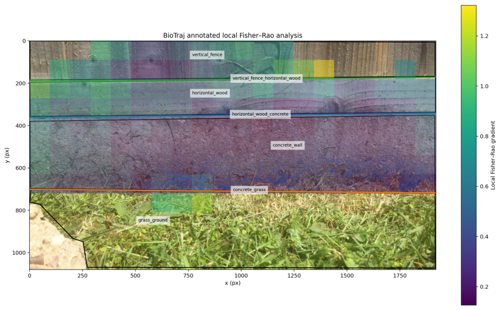
The Wall recording was re-analyzed over the full image domain so that the visible environmental structure was retained. Four surfaces—concrete wall, horizontal wood, vertical fence, and grass/ground—and three corresponding surface transitions were annotated from the first video frame before interpretation of the Fisher–Rao map. The full information-geometric grid was ; 149 cells passed the sampling criterion, and 148 had a defined local gradient.
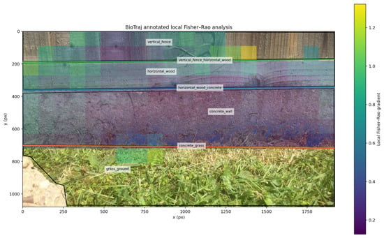
Figure 5 shows the annotated surfaces and transitions overlaid on the local Fisher–Rao field.
Figure 5.
Annotation-aware Fisher–Rao analysis of the Wall recording. Independently defined surface regions and physical transitions are overlaid on the local Fisher–Rao gradient field. The concrete region is dominated by comparatively low local gradients, whereas the horizontal wood and vertical fence contain higher and more heterogeneous values. The grass/ground region contains too few valid cells for quantitative regional comparison.
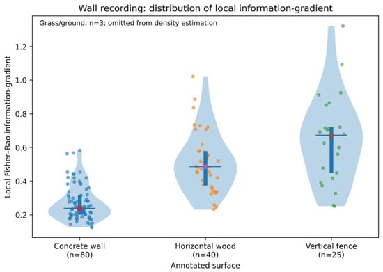
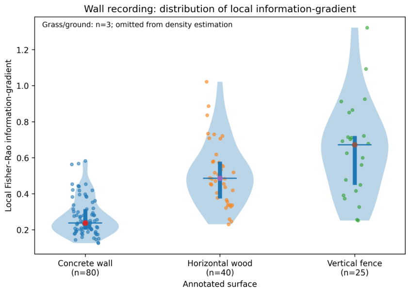
Figure 6 compares the local Fisher–Rao gradients across the adequately sampled surfaces.
Figure 6.
Distribution of local Fisher–Rao gradients by independently annotated surface in the Wall recording. Violin densities are shown for the three adequately sampled surfaces, with individual cell values and summary indicators retained. Cell-level values are descriptive: neighboring cells are spatially dependent and are not treated as independent biological replicates. Grass/ground contained only three valid cells and was therefore not assigned a violin density or used for quantitative regional interpretation.
Among adequately sampled surfaces, local Fisher–Rao heterogeneity differed markedly. The concrete wall had a mean gradient of 0.270 (median 0.238; ), horizontal wood 0.512 (median 0.486; ), and vertical fence 0.648 (median 0.672; ). Only three valid cells were assigned to grass/ground, so that region was not used for quantitative surface comparison. No annotation-defined artifact regions were excluded, and raw and quality-controlled summaries were consequently identical.
The surface transition analysis did not show a universal monotonic decrease in the Fisher–Rao gradient with distance from a boundary. Within one cell width of the annotated transitions, mean gradients were approximately 0.359 for horizontal wood/concrete, 0.336 for concrete/grass, and 0.621 for vertical fence/horizontal wood. The complete distance curves differed among transitions and included sparsely populated distant bins. The Wall recording therefore supports association of the information-geometric field with independently defined macroscopic scene structure but not interpretation of the field as a generic physical edge detector.
The distance-to-transition plot is useful as a diagnostic because it demonstrates that the Fisher–Rao field is not simply an edge detector. However, because distant bins can contain few cells, the full curve is better retained in the Supplementary Materials, together with the bin counts, rather than used as a primary main-text result.
4. Discussion
BioTraj combines video-based trajectory extraction and conventional trajectory descriptors with an information-geometric representation of local and time-resolved movement statistics. These components provide complementary descriptions of trajectory data. Global descriptors characterize properties such as spatial exploration, anisotropy, persistence, and transport, while occupancy maps describe where observations occur. Fisher–Rao analysis instead compares empirical movement distributions and therefore identifies regions or periods in which their statistical character changes.
The simulation-based validation shows that the information-geometric analysis responds reproducibly to deliberately imposed spatial and temporal changes at the resolution defined by the spatial grid and temporal windows. The multi-seed null analysis, parameter sensitivity tests, change magnitude series, and comparison with alternative distributional measures further show that the principal imposed temporal structure is not an artifact of a single random realization or one narrowly selected analysis setting. The comparison does not establish universal superiority of the Fisher–Rao distance over Hellinger, Jensen–Shannon, Wasserstein, or scalar descriptors; these measures have different geometries, scales, and interpretations. The finite-sampling analysis also demonstrates an important limitation: empirical Fisher–Rao distances contain sampling variability, particularly when local trajectory observations are sparse. This dependence should be considered when comparing regions with different occupancies or datasets with substantially different sampling densities.
The Fisher–Rao construction used here is based on established geometric representations of probability distributions, in which square root representations provide a tractable spherical geometry for distributional comparison [21,22]. BioTraj applies this construction to empirical turning angle distributions estimated from different spatial regions or temporal windows and maps the resulting distributional differences back onto the organization of the trajectories.
The experimental recordings illustrate the importance of interpreting these maps together with independently defined scene information. In the Yellow ant recording, the historical footprint of a removed rock was associated with a broad regional difference after controlling for proximity to the tracking boundary, whereas the smaller candidate nest openings were not resolved at the selected spatial scale. In the Wall recording, independently annotated surfaces exhibited different local Fisher–Rao heterogeneity, while distance-from-visible-surface transitions did not show a universal monotonic response.
A local Fisher–Rao difference establishes that estimated movement distributions differ, but does not identify the mechanism responsible for that difference. In field recordings, variation may arise from biological responses, physical constraints, surface geometry and projection, tracking quality, or combinations of these factors. Scene annotation therefore provides context for evaluating detected statistical structure rather than converting it automatically into behavioral classifications. Controlled and replicated experiments would be required to test specific causal relationships.
The approach complements established hidden Markov and state-space methods [8,9]. Such methods are particularly useful when the objective is inference about a finite set of latent states, whereas the present approach compares empirical movement distributions without requiring a predefined number of behavioral states. Spatial cells within a single recording are also not independent biological replicates; the present annotation-aware comparisons are therefore descriptive rather than population-level inferential tests.
Turning angle was selected here as an interpretable local descriptor of trajectory geometry rather than as a complete representation of organism behavior. Other biologically relevant quantities, including turning frequency, run length between successive turns, inter-individual distance, and measures of local alignment, can be derived from trajectories and analyzed separately or incorporated into future extensions of the information-geometric framework. Step length, speed, orientation, and joint distributions are additional possibilities when sampling permits.
Although the examples presented here were recorded using a smartphone camera, the analysis framework is not intrinsically tied to that acquisition device. Video or image sequences obtained using conventional digital cameras, camera traps, drone-mounted cameras, or microscopy can in principle be used provided that suitable two-dimensional trajectories can be extracted. The current BioTraj implementation analyzes two-dimensional image plane trajectories and does not reconstruct three-dimensional motion. A future extension could instead accept externally reconstructed trajectories obtained, for example, from stereovision, depth-resolved microscopy, or other 3D reconstruction methods.
BioTraj also does not require the biological environment itself to have a regular geometry. In complex scenes, independent masks and annotations can define irregular surfaces, obstacles, boundaries, or other regions of interest, while the Fisher–Rao map can be inspected without annotations to identify statistical heterogeneity requiring subsequent contextual interpretation. Approximately planar scenes may be rectified or spatially calibrated when appropriate information is available. In genuinely non-planar environments, however, the present 2D analysis represents a projection of the underlying motion, so physical distances, speeds, and apparent spatial heterogeneity should be interpreted cautiously.
Future developments could also include adaptive spatial partitions, explicit finite-sample calibration, hierarchical or block resampling approaches, and geometric correction where scene calibration permits projection effects to be quantified.
Video-based trajectory studies can also involve sensitive scene, location, or behavioral information. Appropriate storage, access control, anonymization where relevant, and compliance with applicable ethical and data governance requirements should therefore be considered when such recordings are collected or shared. These issues are application-dependent and lie outside the trajectory analysis methodology developed here.
Limitations
Several limitations define the appropriate interpretation of the present analysis: First, empirical Fisher–Rao distances depend on the number of observations used to estimate each histogram, and minimum-count filtering, bootstrap diagnostics, threshold convergence analysis, and equal-count resampling characterize but do not eliminate this dependence. Second, spatial and temporal results depend on histogram resolution, spatial partition, temporal window length, and sampling thresholds, although the synthetic sensitivity analysis shows stable recovery of the imposed transition over the tested ranges. Third, the current unsigned turning angle representation does not retain left–right turning handedness. Fourth, trajectory reconstruction can be affected by poor contrast, object overlap, illumination changes, coordinate error, fragmented tracks, detection gaps, and out-of-plane motion. The additional perturbation, strict continuity, and spatial block bootstrap analyses quantify robustness to selected examples of these effects but do not cover every possible tracking error. Fifth, the current framework analyzes two-dimensional image plane trajectories; motion on oblique or non-planar surfaces can therefore be distorted by camera projection unless independent geometric calibration is available. Finally, spatial cells and temporally adjacent observations within a recording are generally correlated and are not independent biological replicates. Fisher–Rao heterogeneity identifies changes in estimated movement distributions but does not by itself establish discrete behavioral states, biological mechanisms, or causal environmental effects.
5. Conclusions
This study develops and validates an information-geometric approach for detecting spatial and temporal heterogeneity in biological trajectories. Conventional geometric and dynamical descriptors provide complementary characterization of spatial exploration, while local and time-resolved turning angle distributions provide the statistical states compared using Fisher–Rao geometry.
The present work introduces an information-geometric component for detecting spatial and temporal changes in empirical movement distributions. Simulation-based validation demonstrates recovery of deliberately imposed spatial and temporal changes and identifies limitations associated with analysis resolution and finite sampling. Application to experimental ant recordings further shows how Fisher–Rao maps can be considered together with independently defined scene annotations. These examples emphasize the intended interpretation of the method: Fisher–Rao mapping identifies where and when movement statistics change, while the biological or physical origin of those changes requires additional contextual or experimental evidence.
The integration of conventional trajectory descriptors with spatial and temporal Fisher–Rao analysis provides a reproducible approach for identifying distributional heterogeneity in biological motion. More generally, the results demonstrate how information geometry can complement conventional trajectory analysis by quantifying where and when empirical movement distributions change without requiring predefined behavioral states.
Supplementary Materials
The following supporting information can be downloaded at https://www.mdpi.com/article/10.3390/math14214025/s1: Figure S1: Spatial distributions of tracked positions in the four experimental recordings; Figure S2: Spatial occupancy distributions of the four experimental recordings; Figure S3: Comparison of conventional trajectory descriptors across the four experimental recordings; Figure S4: Mean-squared-displacement scaling of the experimental trajectories; Figure S5: Combined spatiotemporal simulation benchmark; Figure S6: Multi-seed stationary-null and transition validation; Figure S7: Comparison with alternative distributional measures; Figure S8: Response to imposed change magnitude; Figure S9: Sensitivity to the minimum spatial sampling threshold; Figure S10: Relationship between spatial sampling and local Fisher–Rao heterogeneity; Figure S11: Equal-sampling control of local Fisher–Rao heterogeneity; Figure S12: Yellow-ant edge-control diagnostic; Figure S13: Robustness to strict frame-to-frame trajectory continuity; Figure S14: Controlled coordinate-perturbation robustness; Figure S15: Spatial-dependence-aware block bootstrap of the Yellow-ant regional contrast; Figure S16: Local Fisher–Rao heterogeneity as a function of distance from independently annotated surface transitions in the Wall recording; Table S1: Conventional trajectory descriptors for the experimental recordings; Table S2: Principal settings used for simulation-based validation and information-geometric analysis; Table S3: Generator specifications required for independent reproduction; Table S4: One-factor-at-a-time sensitivity of the synthetic benchmark to analysis settings; Table S5: Sensitivity of the temporal Fisher–Rao response to imposed change magnitude; Table S6: Edge-controlled Yellow-ant regional summaries; Table S7: Local Fisher–Rao heterogeneity by annotated surface in the Wall recording; Table S8: Local Fisher–Rao heterogeneity within one spatial-cell width of annotated surface transitions; Table S9: Reference information-geometric settings used in the main analyses.
Funding
This research received no external funding.
Institutional Review Board Statement
The study involved video observations of ants on the author’s private property in the UK. Ants are insects and are not protected animals under Section 1 of the UK Animals (Scientific Procedures) Act 1986; therefore, licensing under that Act was not required.
Data Availability Statement
The software developed for trajectory extraction and analysis is freely available through the GitHub repository: https://github.com/DaniloR56/BioTrajectoryAnalysis (accessed on 1 November 2026). The repository contains the complete source code, installation instructions, example videos and trajectory datasets, configuration files, and documentation required to reproduce and test the analysis workflow. The complete trajectory datasets and original video recordings used in this study are not included in full in the public repository and are available from the corresponding author upon reasonable request.
Acknowledgments
During the preparation and revision of this manuscript and the associated software, the author used OpenAI’s ChatGPT (GPT-5 series) for the purposes of software development and code refinement, documentation, language editing, and manuscript preparation. The author reviewed and edited the output and takes full responsibility for the content of this publication. The author also thanks the anonymous reviewers for their careful and constructive comments, which helped improve the clarity, validation, and presentation of the manuscript.
Conflicts of Interest
The author declares no conflicts of interest.
Abbreviations
The following abbreviations are used in this manuscript:
| CSV | Comma-separated values |
| FR | Fisher–Rao |
| MSD | Mean-squared displacement |
| PCA | Principal component analysis |
References
- Turchin, P. Quantitative Analysis of Movement: Measuring and Modeling Population Redistribution in Animals and Plants; Sinauer Associates: Sunderland, MA, USA, 1998. [Google Scholar]
- Codling, E.A.; Plank, M.J.; Benhamou, S. Random walk models in biology. J. R. Soc. Interface 2008, 5, 813–834. [Google Scholar] [CrossRef] [Scilit] [PubMed]
- Berg, H.C. Random Walks in Biology; Princeton University Press: Princeton, NJ, USA, 1993. [Google Scholar]
- Romanczuk, P.; Bär, M.; Ebeling, W.; Lindner, B.; Schimansky-Geier, L. Active Brownian particles: From individual to collective stochastic dynamics. Eur. Phys. J. Spec. Top. 2012, 202, 1–162. [Google Scholar]
- Szeliski, R. Computer Vision: Algorithms and Applications; Springer: Cham, Switzerland, 2022. [Google Scholar]
- Bradski, G. The OpenCV Library. Dr. Dobb’s J. Softw. Tools 2000, 25, 120–123. [Google Scholar] [CrossRef] [Scilit]
- Bradski, G.; Kaehler, A. Learning OpenCV: Computer Vision with the OpenCV Library; O’Reilly Media, Inc.: Sebastopol, CA, USA, 2008. [Google Scholar]
- Langrock, R.; King, R.; Matthiopoulos, J.; Thomas, L.; Fortin, D.; Morales, J.M. Flexible and practical modeling of animal telemetry data: Hidden Markov models and extensions. Ecology 2012, 93, 2336–2342. [Google Scholar] [CrossRef] [Scilit] [PubMed]
- McClintock, B.T.; Langrock, R.; Gimenez, O.; Cam, E.; Borchers, D.L.; Glennie, R.; Patterson, T.A. Uncovering ecological state dynamics with hidden Markov models. Ecol. Lett. 2020, 23, 1878–1903. [Google Scholar] [CrossRef] [Scilit] [PubMed]
- Amari, S.I. Information Geometry and Its Applications; Applied Mathematical Sciences; Springer: Tokyo, Japan, 2016; Volume 194. [Google Scholar] [CrossRef] [Scilit]
- Nielsen, F. An Elementary Introduction to Information Geometry. Entropy 2020, 22, 1100. [Google Scholar] [CrossRef] [Scilit] [PubMed]
- Byrne, S.; Girolami, M. Geodesic Monte Carlo on Embedded Manifolds. Scand. J. Stat. 2013, 40, 825–845. [Google Scholar] [CrossRef] [Scilit] [PubMed]
- Tinevez, J.Y.; Perry, N.; Schindelin, J.; Hoopes, G.M.; Reynolds, G.D.; Laplantine, E.; Bednarek, S.Y.; Shorte, S.L.; Eliceiri, K.W. TrackMate: An open and extensible platform for single-particle tracking. Methods 2017, 115, 80–90. [Google Scholar] [CrossRef] [Scilit] [PubMed]
- Rodriguez, A.; Zhang, H.; Klaminder, J.; Brodin, T.; Andersson, P.; Andersson, M. ToxTrac: A fast and robust software for tracking organisms. Methods Ecol. Evol. 2018, 9, 460–464. [Google Scholar] [CrossRef] [Scilit]
- Mathis, A.; Mamidanna, P.; Cury, K.M.; Abe, T.; Murthy, V.N.; Mathis, M.W.; Bethge, M. DeepLabCut: Markerless pose estimation of user-defined body parts with deep learning. Nat. Neurosci. 2018, 21, 1281–1289. [Google Scholar] [CrossRef] [Scilit]
- Romero-Ferrero, F.; Bergomi, M.G.; Hinz, R.C.; Heras, F.J.; de Polavieja, G.G. idtracker.ai: Tracking all individuals in small or large collectives of unmarked animals. Nat. Methods 2019, 16, 179–182. [Google Scholar] [CrossRef] [Scilit] [PubMed]
- Jolliffe, I.T.; Cadima, J. Principal component analysis: A review and recent developments. Philos. Trans. R. Soc. A Math. Phys. Eng. Sci. 2016, 374, 20150202. [Google Scholar] [CrossRef] [Scilit] [PubMed]
- Bechinger, C.; Di Leonardo, R.; Löwen, H.; Reichhardt, C.; Volpe, G.; Volpe, G. Active particles in complex and crowded environments. Rev. Mod. Phys. 2016, 88, 045006. [Google Scholar] [CrossRef] [Scilit]
- Fourcassié, V.; Coughlin, D.; Traniello, J.F. Fractal analysis of search behavior in ants. Naturwissenschaften 1992, 79, 87–89. [Google Scholar] [CrossRef] [Scilit]
- Turchin, P. Fractal analyses of animal movement: A critique. Ecology 1996, 77, 2086–2090. [Google Scholar] [CrossRef] [Scilit]
- Kurtek, S.; Bharath, K. Bayesian sensitivity analysis with the Fisher–Rao metric. Biometrika 2015, 102, 601–616. [Google Scholar] [CrossRef] [Scilit]
- Goh, A.; Lenglet, C.; Thompson, P.M.; Vidal, R. A nonparametric Riemannian framework for processing high angular resolution diffusion images and its applications to ODF-based morphometry. NeuroImage 2011, 56, 1181–1201. [Google Scholar] [CrossRef] [Scilit] [PubMed]

Disclaimer/Publisher’s Note: The statements, opinions and data contained in all publications are solely those of the individual author(s) and contributor(s) and not of MDPI and/or the editor(s). MDPI and/or the editor(s) disclaim responsibility for any injury to people or property resulting from any ideas, methods, instructions or products referred to in the content. |
© 2026 by the author. Licensee MDPI, Basel, Switzerland. This article is an open access article distributed under the terms and conditions of the Creative Commons Attribution (CC BY) license.