Forecasting Non-Fungible Token (NFT) Market Volatility Through Hybrid GARCH–LSTM Models

Abstract

This study forecasts price volatility in the non-fungible token (NFT) digital asset market. We develop a hybrid forecasting framework that integrates long short-term memory (LSTM) networks with a set of generalized autoregressive conditional heteroskedasticity (GARCH)-type models. Using daily data, we conduct a comparative evaluation of nine competing forecasting models across five representative NFT submarkets (i.e., OpenSea, Atomic, CryptoKitties, Gods Unchained, and Decentraland). Employing standard error metrics (RMSE, MSE, MAE, and RAE), a robust loss QLIKE function, and the Diebold–Mariano (DM) statistical test, our empirical results show that the hybrid GARCH-TGARCH-LSTM model achieves the lowest error metrics. Compared with the baseline LSTM model, it achieves RMSE reductions of approximately 14% for Atomic, 49% for CryptoKitties, 13% for Decentraland, 8% for Gods Unchained, and 29% for OpenSea. Furthermore, the EGARCH conditional variance specification underperforms the TGARCH counterpart in the most NFT submarkets. This finding suggests that combining the volatility clustering characteristics captured by standard GARCH models with the asymmetric volatility features captured by TGARCH models improves forecasting performance. This study contributes to research on hybrid deep learning approaches to volatility forecasting in emerging digital asset markets.

1. Introduction

The global economy is undergoing rapid digital transformation alongside the expansion of the Web 3.0 ecosystem. Against this backdrop, non-fungible tokens (NFTs) have experienced rapid growth, evolving from simple tools that represented ownership of digital art into digital assets with broader financial applications. As blockchain-based assets integrate into the digital financial system, the stability and long-term development of these emerging markets have become increasingly important. The underlying blockchain technology is maturing and increasingly integrating with decentralized finance (e.g., the rise of NFTFi). This was accompanied by substantial increases in the market capitalization of top NFT collections over several months, with secondary-market trading volumes repeatedly surpassing $1 billion [1]. However, the high returns in the NFT market are often accompanied by extreme volatility and complex price dynamics—characteristics that are more pronounced than those observed in traditional financial assets [2]. Due to the lack of a centralized regulatory framework and a continuous order book mechanism, this market exhibits pronounced price discontinuities and irregular trading intervals. Consequently, the market is highly susceptible to sudden and sharp fluctuations triggered by factors such as changes in the macroeconomic environment or a breakdown in community consensus. The NFT market typically displays sharp price jumps and volatility clustering, which pose challenges for accurate time-series modeling and statistical forecasting [3].

NFTs represent unique blockchain-based digital certificates, exhibiting non-fungibility and relatively weak market liquidity. Crucially, the absence of market makers implies that NFT trading typically relies on multi-round bargaining, with prices revealed only on transaction days. Consequently, many NFT markets lack a continuous order book, resulting in highly discontinuous price time series. This market structure amplifies the inherent stylized facts of financial assets. For instance, Fama [4] proposed “leptokurtosis,” while Mandelbrot [5] and Morgan [6] discovered “volatility clustering” and time-varying heteroskedasticity. These phenomena are particularly pronounced in the NFT market. Furthermore, Black [7] revealed a “leverage effect” in traditional stock markets. A similar dynamic has been observed in the NFT market [8]. The NFT market features a complex microstructure, which is intertwined with discontinuous trading and extreme heteroskedasticity. Existing evidence shows that the NFT market is characterized by highly concentrated trading activity, heterogeneous transaction patterns, and complex interactions among market participants, all of which contribute to market instability and uncertainty [9]. Therefore, effectively modeling and accurately forecasting the asymmetric volatility of NFTs has become an important challenge.

Numerous studies have investigated approaches to forecasting the volatility of financial time series, including Generalized Autoregressive Conditional Heteroskedasticity (GARCH)-type models, deep learning methods, and hybrid architectures combining both. These methods have demonstrated great predictive performance in traditional asset markets with continuous prices. However, existing research on emerging digital assets such as NFTs has primarily focused on identifying cross-sectional pricing factors and uncovering microstructural behaviors such as herding. Currently, systematic research on the dynamic forecasting of NFT price time series remains limited, and the applicability of hybrid deep learning architectures in such highly volatile and price-discontinuous markets remains to be rigorously examined. Therefore, this study aims to apply hybrid models to the NFT market. A GARCH-LSTM hybrid framework is constructed to forecast the price volatility of five representative NFT submarkets (OpenSea, Atomic, CryptoKitties, Gods Unchained, and Decentraland). The contributions to digital asset volatility prediction are threefold:

(1)

This paper extends the application of existing hybrid deep neural networks. Specifically, it addresses a research gap by systematically comparing the forecasting performance of different GARCH-LSTM hybrid models for NFT price volatility.

(2)

This research evaluates the robustness of the proposed forecasting model across five distinct NFT submarkets. By examining NFT submarkets with heterogeneous underlying blockchain architectures and diverse application scenarios, this study provides empirical evidence on the applicability and robustness of the hybrid forecasting framework across different digital asset markets.

(3)

This paper further examines the heterogeneous performance of different model input mechanisms in capturing asymmetric volatility characteristics within NFT submarkets. The empirical results demonstrate that conditional variance features extracted from the TGARCH model outperform those derived from the EGARCH model when serving as LSTM inputs. The TGARCH-based hybrid framework shows better performance in capturing asymmetric market shocks under the discontinuous pricing environment of NFT assets.

2. Literature Review

2.1. Volatility Modeling: From GARCH-Type Models to Deep Learning Methods

GARCH-type models have long served as fundamental approaches for modeling financial volatility. Introduced by Engle [10] and extended by Bollerslev [11], these models incorporate autoregressive dynamics into conditional variance, thereby effectively capturing the clustering effects of volatility. Their applicability has been extensively validated in both traditional and emerging financial markets [12,13,14]. Subsequent extensions, such as EGARCH and TGARCH, have further refined the ability to model asymmetric volatility characteristics triggered by different shocks. Comparative studies by Hansen and Lunde [15] and Alberg et al. [16] have demonstrated the usefulness of these models when dealing with assets exhibiting significant leverage effects. However, traditional GARCH-type models depend on prespecified model structures and distributional assumptions, which may limit their capability to characterize nonlinear volatility patterns, price jumps, and complex market noise.

Therefore, deep learning methods have been increasingly incorporated to enhance nonlinear forecasting capabilities. Among these, long short-term memory (LSTM) networks leverage memory cells and gating structures to selectively preserve historical information, enabling them to effectively characterize complex financial time series [17]. Compared to traditional econometric models, LSTM offers greater flexibility and requires fewer assumptions about the underlying data generation process. Nevertheless, purely data-driven models are limited in terms of economic interpretability and may fail to explicitly incorporate established volatility characteristics—which are particularly pronounced in the NFT market. Therefore, the respective strengths and limitations of GARCH-type models and deep learning models provide a theoretical basis for developing a hybrid volatility forecasting framework.

2.2. Hybrid Architectures: Econometrics and Deep Learning

Hybrid architectures combine the rigor of econometrics in feature extraction with the nonlinear pattern recognition capabilities of deep learning. In recent years, this integration has become an active research area in financial forecasting and has continued to evolve. Early work by Donaldson and Kamstra [18] combined artificial neural networks with GARCH models. Subsequently, Kim and Won [19] combined LSTM networks with various GARCH-type models. More recently, Pan et al. [20] applied a multi-GARCH-LSTM approach to forecast stock index futures prices.

Hybrid architectures typically use the time-varying conditional variances generated by GARCH-type models as additional input features for the network. Several studies indicate that this architecture can improve generalizability and forecasting accuracy. The method has shown broad applicability across diverse interdisciplinary domains, including traditional stock indices [21], commodities like highly volatile copper prices [22], and environmental science [23,24]. More importantly, researchers have explored the cryptocurrency market, an emerging digital asset class similar to NFTs. In-depth studies by Gao et al. [25] and Amirshahi and Lahmiri [26] provided strong evidence. Their findings suggest that the GARCH-LSTM framework helps capture volatility patterns in the presence of short-term market noise in crypto assets. Consequently, this approach effectively improves the out-of-sample volatility forecasting performance for mature cryptocurrencies like Bitcoin.

2.3. NFT Market Microstructure and Existing Research Gaps

NFTs are unique digital assets, characterized by non-fungibility, a lack of standardized underlying assets, and discontinuous trading. Consequently, a substantial body of early research has focused on their cross-sectional pricing characteristics and investment properties. Studies by Maouchi et al. [27] and Schaar and Kampakis [28] positioned NFTs as an alternative investment, highlighting their unique market dynamics and susceptibility to speculative bubbles. Other studies have examined specific pricing factors within the digital art ecosystem. Horky et al. [29] systematically identified price determinants related to digital scarcity. Additionally, Nguyen [30] examined more granular features to reveal price variations associated with specific visual attributes, such as skin tone in CryptoPunks. More recently, Kang and Oh [31] decoded NFT valuation premiums by examining the cognitive impact of name fluency on digital artworks. Beyond static pricing models, another strand of research involves qualitative exploration and empirical analysis of trading behaviors. Bao et al. [32] provided empirical evidence of widespread herding effects across the NFT landscape. This line of inquiry was further advanced by Fridgen et al. [33], who conducted an in-depth study confirming that pricing dynamics are influenced by sentiment-driven herding behavior.

A growing literature has also investigated the dynamic return and volatility characteristics of NFT markets and their linkages with other financial and cryptocurrency markets. Dowling [34] examined the relationship between NFT and cryptocurrency prices and found limited volatility transmission but evidence of co-movement between the two markets. Aharon and Demir [35] investigated return connectedness between NFTs and traditional financial assets as well as Ethereum, showing that NFT returns are largely driven by specific shocks and exhibit time-varying spillover relationships with other asset classes. At the NFT-segment level, Umar et al. [36] documented heterogeneous return and volatility spillovers across different NFT categories, identifying distinct transmitter and receiver roles among NFT segments. Similarly, Yousaf and Yarovaya [37] analyzed the dynamic connectedness between NFTs, DeFi assets, and other financial markets and showed that return and volatility spillovers vary substantially over time and across market conditions.

Although these studies have advanced the understanding of NFT volatility, connectedness, and cross-market spillovers, their primary focus is not on systematically evaluating out-of-sample volatility forecasting models. This study differs from the literature by focusing specifically on volatility forecasting at the NFT submarket level. In particular, this paper systematically compares nine forecasting models across five heterogeneous NFT submarkets and evaluates whether combining GARCH-family volatility features with LSTM networks improves predictive performance. This research provides empirical evidence on the forecasting value of integrating econometric volatility structures with nonlinear deep learning architectures for highly discontinuous NFT markets.

3. Methodology

3.1. Generalized Autoregressive Conditional Heteroskedasticity (GARCH) Model

The volatility of financial time series typically exhibits specific characteristics, including time-varying dynamics, clustering, and long-memory properties. Traditional time series analysis assumes constant residual variance, while heteroskedasticity in financial data violates this assumption. To address this issue, Bollerslev [11] introduced the Generalized Autoregressive Conditional Heteroskedasticity (GARCH) model. This model captures volatility persistence and time-varying conditional variance, thereby capturing the widely observed volatility clustering phenomenon. The GARCH (p, q) model is used to extract the underlying volatility dynamics. This model consists of a mean equation and a conditional variance equation, expressed as follows:

$$y_t=\mu +{\epsilon }_t$$

(1)

$${\sigma }_t^2=w+{\displaystyle {\displaystyle \sum _{i=1}^q}{\alpha }_i{\epsilon }_{t-i}^2}+{\displaystyle {\displaystyle \sum _{j=1}^p}{\beta }_j{\sigma }_{t-j}^2}$$

(2)

where ${\sigma }_t^2$ is the time-varying conditional variance at time $t$, which will later serve as a key input feature into the LSTM network, and $w$ is a constant term (>0). ${\alpha }_i$ and ${\beta }_j$ denote the coefficients of the ARCH and GARCH components, respectively, and are required to be non-negative to guarantee a non-negative conditional variance. Throughout this study, p denotes the lag order of the conditional-variance terms, whereas q denotes that of the squared residuals.

A standard GARCH framework assumes a symmetric response of volatility to shocks of equal magnitude, irrespective of whether they are positive or negative. However, in emerging digital asset markets, the impact of shocks is often asymmetric. Such an asymmetric response is commonly associated with the leverage effect. To capture this asymmetric shock response in the NFT market, this study further introduces the TGARCH and EGARCH models.

3.2. Threshold GARCH (TGARCH) Model

To account for the asymmetric response of conditional volatility to shocks of different signs, Glosten et al. [38] developed the Threshold GARCH (TGARCH) model. By incorporating an indicator function, this model can capture the different effects of positive and negative shocks on conditional variance. The conditional variance equation under the TGARCH (p, q) specification is expressed as follows:

$${\sigma }_t^2=w+{\displaystyle {\displaystyle \sum _{i=1}^q}({\alpha }_i+{\gamma }_i{N}_{t-i})}{\epsilon }_{t-i}^2+{\displaystyle {\displaystyle \sum _{j=1}^p}{\beta }_j}{\sigma }_{t-j}^2$$

(3)

$$N_{t-i}=\left\{\begin{array}{l}1, {\epsilon }_{t-i}<0,\\ 0, {\epsilon }_{t-i}\ge 0.\end{array}\right.$$

(4)

where w denotes the constant component of conditional variance, ${\alpha }_i$ corresponds to the coefficient on the lagged squared error term, and ${\beta }_j$ is the coefficient on the lagged conditional variance term. Asymmetry is captured by ${\gamma }_i{N}_{t-i}$, where the indicator variable $N_{t-i}$ distinguishes negative shocks from positive ones. Consequently, the effect of a positive shock is determined by ${\alpha }_i$, whereas an equally sized negative shock has an overall coefficient of ${\alpha }_i+{\gamma }_i$. A positive value of ${\gamma }_i$ therefore implies a stronger volatility reaction to negative shocks and provides a direct representation of the leverage effect. The lag orders p and q follow the convention established in Section 3.1. The resulting specification models the temporal evolution of conditional variance for an individual series.

3.3. Exponential GARCH (EGARCH) Model

Nelson [39] introduced the Exponential GARCH (EGARCH) model. This model directly specifies the natural logarithm of the conditional variance. Consequently, it eliminates the need to impose non-negativity constraints on the model parameters. Furthermore, it allows positive and negative shocks to have asymmetric effects on volatility. The specific mathematical form of EGARCH (p, q) is defined as

$$r_t=X_t\beta +{\epsilon }_t$$

(5)

$$\ln {\sigma }_t^2=w+{\displaystyle {\displaystyle \sum _{i=1}^q}\left[{\alpha }_i(\left|z_{t-i}\right|-\sqrt{\frac{2}{\pi }})+{\gamma }_i{z}_{t-i}\right]}+{\displaystyle {\displaystyle \sum _{j=1}^p}{\beta }_j}\ln {\sigma }_{t-j}^2$$

(6)

where ${\sigma }_t^2$ denotes the conditional variance, and $z_{t-i}={\displaystyle \frac{{\epsilon }_{t-i}}{{\sigma }_{t-i}}}$ represents the standardized innovation. The constant w signifies the constant term in the log-variance equation, ${\alpha }_i$ represents the coefficient on lagged innovations, and ${\beta }_j$ governs the lagged conditional-variance coefficient. The parameter ${\gamma }_i$ captures the asymmetric effects of positive and negative innovations. The term $\sqrt{{\displaystyle \frac{2}{\pi }}}$ represents the expected absolute value of a standard normal innovation. The lag-order convention remains consistent with that adopted in Section 3.1. By formulating conditional variance in logarithmic form, EGARCH guarantees a positive variance without imposing the non-negativity constraints commonly applied to the variance coefficients of standard GARCH models. This univariate model is thus suitable for modeling the conditional volatility of a single time series.

3.4. Long Short-Term Memory (LSTM) Neural Network

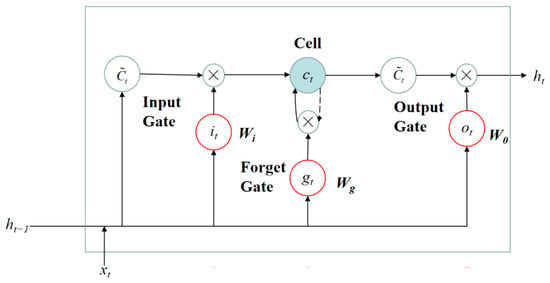
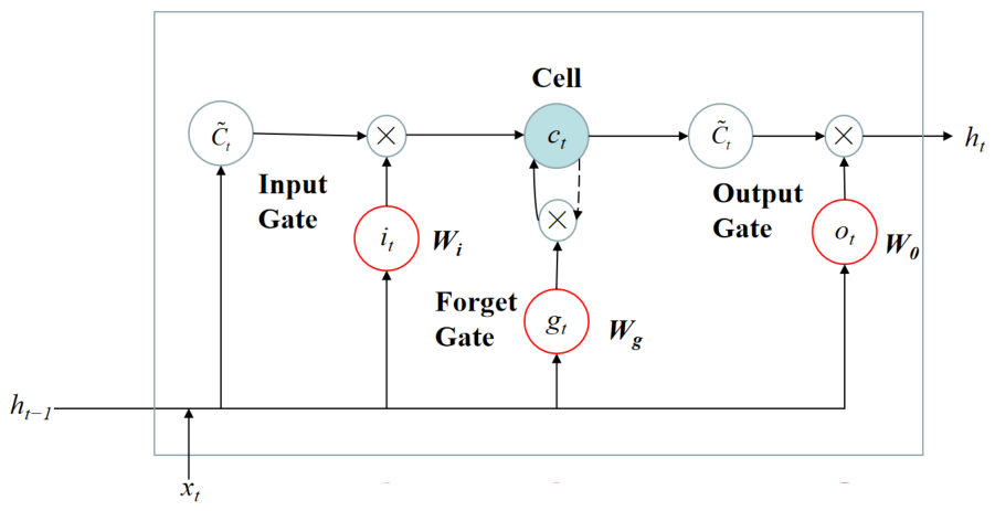
Standard Recurrent Neural Networks (RNNs) suffer from a well-recognized limitation: during backpropagation over long time spans, gradients may vanish or explode, thus preventing the model from capturing long-term sequential dependencies [40]. To address this limitation, the long short-term memory (LSTM) network introduces a dedicated memory cell and three gating mechanisms: the forget gate, the input gate, and the output gate. The structure of the LSTM unit is illustrated in Figure 1. The information flow and state updates within the LSTM unit are governed by the following equations [41]:

Figure 1. Schematic diagram of the LSTM unit.

(1)

Forget Gate: Based on the previous hidden state $h_{t-1}$ and current input $x_t$, it decides which useless information to discard from the long-term memory.

$$g_t=\sigma (W_g\left[h_{t-1},x_t\right]+b_g)$$

(7)

(2)

Input Gate and Candidate Cell: These decide which new information will be selectively stored in the cell state.

$$i_t=\sigma (W_i\left[h_{t-1},x_t\right]+b_i)$$

(8)

$${\tilde{c}}_t=\tanh (W_c\left[h_{t-1},x_t\right]+b_c)$$

(9)

(3)

Cell State Update: This step combines the old cell state with newly extracted information to update the current state $c_t$.

$$c_t=g_t\odot c_{t-1}+i_t\odot {\tilde{c}}_t$$

(10)

(4)

Output Gate: This determines the final hidden layer output feature based on the updated cell state.

$$o_t=\sigma (W_o[h_{t-1},x_t]+b_o)$$

(11)

$$h_t=o_t\odot \tanh (c_t)$$

(12)

In these equations, $\sigma$ represents the Sigmoid activation function, and $\tanh$ represents the hyperbolic tangent activation function. $W$ and $b$ denote the weight matrices and bias terms for each gate, respectively. By synergistically retaining long-term information and filtering short-term noise, LSTM effectively models the complex dependencies of long-range time series. It should be noted that ${\tilde{c}}_t$ denotes the candidate cell state, whereas $c_t$ represents the updated cell state. These two quantities are distinguished by the tilde notation.

3.5. Hybrid Model Architecture (GARCH-LSTM Framework)

Deep learning and GARCH-type models possess complementary advantages in volatility forecasting. GARCH-type models are effective at extracting volatility-related features. They can capture volatility persistence and leverage effects under market shocks, serving as useful feature extractors. Conversely, LSTM deep learning models possess flexible nonlinear modeling capabilities without requiring the same distributional assumptions as traditional econometric models.

Consequently, this study constructs hybrid forecasting architectures (GARCH-LSTM). The dynamic outputs from the GARCH-type models are added to the input layer of the LSTM model as additional features. Specifically, the parameters of the GARCH-type models are first estimated using the training dataset. The GARCH-derived features fed into the LSTM refer exclusively to the extracted time-varying conditional variance series (${\sigma }_t^2$), rather than static model coefficients. The input vector dimension ranges from 3 to 6. The basic input feature vector ($X_{Base,t}$) comprises three features at each time step, including the historical log return, squared return, and absolute return:

$$X_{Base,t}=\left[R_{t-1},R_{t-1}^2,\left|R_{t-1}\right|\right]$$

(13)

Building upon this, the hybrid models concatenate the time-varying conditional variances (denoted as ${\sigma }_{G,t}$, ${\sigma }_{TG,t}$, and ${\sigma }_{EG,t}$ for GARCH, TGARCH, and EGARCH, respectively) as additional features. For instance, the input vector for the GARCH-LSTM model is explicitly formulated as follows:

$$X_{GARCH\text{-}LSTM,t}=\left[R_{t-1},R_{t-1}^2,\left|R_{t-1}\right|,{\sigma }_{G,t}\right]$$

(14)

This configuration is consistent with the settings proposed by Shu et al. [42]. This study adopts the rolling-window sample standard deviation of daily logarithmic returns as the proxy variable for volatility, denoted by ${\sigma }_{\mathrm{t}}^{\mathrm{roll}}$. Given the heterogeneity in asset lifespans and trading frequencies across the NFT market, the model embeds a data-adaptive mechanism. Based on the effective sample size (N), the model dynamically adjusts the rolling-window length and the LSTM lookback size, ranging adaptively from 4 to 30 observations. This method is designed to avoid look-ahead bias by using only past observations during forecasting. It also aims to balance feature sensitivity for small-sample assets with long-term memory for large-sample assets.

To ensure rigorous model evaluation, all data preprocessing, GARCH-type coefficient estimation, hyperparameter optimization, and early stopping procedures are strictly confined to the training set. The conditional variance series are generated recursively using parameters estimated from the training set and subsequently held fixed. Feature scaling is fitted exclusively on the training data. Finally, by learning these composite sequential variables, the LSTM network can capture temporal dependencies and mitigate the influence of noise. This improves the model’s overall performance in forecasting volatility within a highly discontinuous asset market like NFTs. The test set is accessed strictly only once during the final evaluation stage.

3.6. Forecasting Target, Evaluation Metrics, and Statistical Test

3.6.1. Rolling-Window Volatility Proxy

Given the pronounced price discontinuity in the NFT market and the constraint of daily-level data, conventional realized variance cannot be constructed. Therefore, this study adopts the rolling-window sample standard deviation of daily logarithmic returns as a proxy for volatility. This measure captures the dispersion of daily returns within a historical window and is therefore referred to as the rolling-window volatility proxy. Brownlees and Gallo [43] compared alternative volatility measures from a risk management perspective, highlighting the importance of volatility measurement choices for forecasting applications. Unlike conventional realized volatility measures constructed from high-frequency returns, the rolling-window estimator may not fully capture rapid changes in the underlying volatility process. In particular, the rolling-window aggregation may smooth abrupt volatility fluctuations and introduce delayed responses to sudden market shocks. Consequently, the resulting measure is regarded as an approximation of the underlying volatility dynamics rather than a direct observation of the latent conditional volatility.

The rolling-window volatility proxy at time t, denoted by ${\sigma }_{\mathrm{t}}^{\mathrm{roll}}$, is calculated using the sample standard deviation of returns within the corresponding window. To prevent look-ahead bias, the rolling-window volatility proxy at time $t$ is calculated solely using historical data up to time $t$. The calculation is based on the rolling-window mean return, defined in Equation (16), and the resulting volatility proxy is given by Equation (15).

$${\sigma }_t^{roll}=\sqrt{{\displaystyle \frac{1}{w-1}}{\displaystyle \sum _{i=0}^{w-1}{(R_{t-i}-{\overline{R}}_t)}^2}}$$

(15)

where $w$ represents the dynamic rolling window size (adaptively configured between 4 and 30 observations based on the asset’s effective sample size), $R_{t-i}$ is the logarithmic return, and ${\overline{R}}_t$ is the mean return over the rolling window:

$${\overline{R}}_t={\displaystyle \frac{1}{w}}{\displaystyle \sum _{i=0}^{w-1}{R}_{t-i}}$$

(16)

3.6.2. Error Evaluation Metrics

To evaluate the out-of-sample forecasting performance of the models, the following five evaluation metrics are employed: Root Mean Square Error (RMSE), Mean Squared Error (MSE), Mean Absolute Error (MAE), Relative Absolute Error (RAE), and the QLIKE loss function.

Let $N$ be the total number of observations in the out-of-sample test set. Let $y_t={\sigma }_{\mathrm{t}}^{\mathrm{roll}}$ represent the observed rolling-window volatility proxy, and ${\widehat{y}}_t={\widehat{\sigma }}_{\mathrm{t}}^{\mathrm{roll}}$ denote the corresponding volatility forecast. RMSE, MSE, MAE, and RAE are calculated directly using the observed and predicted volatility values. In contrast, QLIKE evaluates forecasts on the variance scale. Accordingly, the observed variance proxy is $y_t^2$, while the predicted variance is ${\widehat{y}}_t^2$. The following metrics are used to evaluate the out-of-sample forecasting performance of the models.

(1)

Root Mean Square Error (RMSE)

$$RMSE=\sqrt{{\displaystyle \frac{1}{N}}{\displaystyle \sum _{t=1}^N{(y_t-{\widehat{y}}_t)}^2}}$$

(17)

(2)

Mean Squared Error (MSE)

$$MSE={\displaystyle \frac{1}{N}}{\displaystyle \sum _{t=1}^N{(y_t-{\widehat{y}}_t)}^2}$$

(18)

(3)

Mean Absolute Error (MAE)

$$MAE={\displaystyle \frac{1}{N}}{\displaystyle \sum _{t=1}^N\left|y_t-{\widehat{y}}_t\right|}$$

(19)

(4)

Relative Absolute Error (RAE)

RAE measures the model’s predictive error relative to a naive baseline forecast (which uses the mean target value from the training set, ${\overline{y}}_{train}$):

$$RAE={\displaystyle \frac{{\displaystyle {\sum }_{t=1}^N\left|y_t-{\widehat{y}}_t\right|}}{{\displaystyle {\sum }_{t=1}^N\left|y_t-{\overline{y}}_{train}\right|}}}$$

(20)

(5)

QLIKE Loss Function

Following Patton [44], the QLIKE loss function is employed to evaluate conditional variance forecasts when the underlying volatility is unobservable and is approximated using an imperfect proxy. In this study, QLIKE is calculated using the squared rolling-window volatility proxy and the squared predicted volatility. It is highly robust to noisy volatility proxies and heavily penalizes under-predictions. However, this robustness property depends on assumptions concerning the proxy, particularly its conditional unbiasedness for the latent variance. Since rolling-window standard deviations derived from NFT returns may contain smoothing errors, estimation noise, or systematic biases associated with irregular trading, these conditions cannot be assumed to hold exactly. Therefore, this paper uses QLIKE as a complementary evaluation criterion rather than as a measurement-error-free assessment of forecasting accuracy. The QLIKE loss function is expressed as follows:

$$QLIKE={\displaystyle \frac{1}{N}}{\displaystyle \sum _{t=1}^N(\ln ({\widehat{y}}_t^2)+\frac{y_t^2}{{\widehat{y}}_t^2})}$$

(21)

(6)

Confidence Intervals for RMSE

To quantify the uncertainty associated with out-of-sample forecasting performance, 95% confidence intervals for RMSE are estimated using a circular block bootstrap procedure with 2000 replications. The same bootstrap time indices are applied to all competing models within each submarket to ensure a consistent basis for comparison. These confidence intervals reflect the uncertainty in the estimated out-of-sample RMSE conditional on the fitted models and observed forecasts.

3.6.3. DM Statistical Test

The Diebold–Mariano (DM) test is employed to examine whether the predictive accuracy of competing forecasting models differs significantly [45]. This study conducts model comparisons using squared prediction errors as the loss function. The DM statistic is defined as follows:

$$D{M}_{ij}={\displaystyle \frac{{\overline{d}}_{ij}}{\sqrt{{\widehat{\mathsf{\Omega }}}_{ij}/T}}}$$

(22)

where ${\overline{d}}_{ij}$ denotes the mean loss differential between models (i) and (j), defined as $d_{ij,t}={(y_t-{\widehat{y}}_{i,t})}^2-{(y_t-{\widehat{y}}_{j,t})}^2$. T is the number of out-of-sample observations, and ${\widehat{\mathsf{\Omega }}}_{ij}$ represents the estimated long-run variance of the loss differential series.

To account for potential heteroskedasticity and serial correlation, the long-run variance is estimated using the Newey–West heteroskedasticity and autocorrelation consistent (HAC) estimator with Bartlett kernel weights:

$${\hat{\mathsf{\Omega }}}_{ij}={\widehat{y}}_0+2{\displaystyle \sum _{k=1}^L(1-\frac{k}{L+1})}{\widehat{y}}_k$$

(23)

where ${\widehat{y}}_k$ denotes the sample autocovariance at lag k, and L is the truncation lag selected according to $L=\min \left\{T-2,\max [1,w-1,⌊4{({\displaystyle \frac{T}{100}})}^{2/9}⌋]\right\}$, with w denoting the rolling-window length used to construct the volatility proxy.

4. Empirical Analysis and Results

4.1. Data Sources and Preprocessing

The dataset used in this study was compiled by Nadini et al. [9], which is publicly available at https://osf.io/wsnzr/?view_only=319a53cf1bf542bbbe538aba37916537 accessed on 25 July 2022) The raw dataset comprises over six million transaction records, covering the period from 23 November 2017 to 27 April 2021, across five NFT submarkets: OpenSea, Atomic, CryptoKitties, Gods Unchained, and Decentraland. The selected period encompasses the early development of the NFT ecosystem and the initial acceleration of market activity, during which NFT trading was characterized by relatively limited liquidity, discontinuous transactions, and pronounced price fluctuations. These markets exhibit differences in their underlying blockchain architectures, asset types, and user demographics, reflecting the diversity of the NFT ecosystem. The primary objective of this paper is to investigate the relative forecasting performance of different hybrid models during this early stage of NFT market development, providing a historical benchmark for volatility forecasting in emerging digital asset markets.

The NFT market often exhibits pronounced price discontinuity. Without centralized market makers, transactions occur intermittently between buyers and sellers, meaning prices are revealed only on the exact days when transactions occur. Consequently, aggregating individual transactions into a continuous time series requires careful preprocessing. Following the methodology proposed by Bao et al. [32], the data cleaning and daily return construction processes are detailed as follows:

(1)

Currency Standardization: Although tokens are primarily priced in Ethereum, an equivalent US dollar value is provided for each transaction. To ensure consistency across different submarkets and time periods, the US dollar value of each transaction is uniformly adopted for return calculations.

(2)

Handling Several Within-Day Transactions: For NFTs that experience multiple transactions within a single day $t$, the transactions are sorted chronologically. The price of the first transaction is selected as the daily opening price ($P_t^o$), and the price of the last transaction is designated as the daily closing price ($P_t^e$). The within-day logarithmic return is then calculated as follows:

$$R_{i,t}=\ln (P_t^e)-\ln (P_t^o)$$

(24)

(3)

Handling No-Trading Days (Cross-Day Returns): For days with no trading activity, the pricing table becomes unbalanced. To resolve the missing values without introducing artificial noise, the cross-day return is calculated. If an NFT trades on day $t$ and then remains untraded until day $t^{\prime }$, the return across this illiquid gap is formulated as follows:

$$R_{i,t^{\prime }-1}={\displaystyle \frac{\ln (P_{t^{\prime }}^o)-\ln (P_t^e)}{t^{\prime }-t}}$$

(25)

In this equation, $P_{t^{\prime }}^o$ is the open price of the next available trading day, and $P_t^e$ is the end price of the last trading day. This method systematically calculates the total logarithmic price difference across the gap and divides it by the number of elapsed days ($t^{\prime }-t$). By evenly distributing the return across the no-trading period and assigning it to the day of the next trade, this approach maximizes the utilization of available information while accurately reflecting the long-term illiquidity characteristics of the NFT market.

It should be noted that the empirical analysis considers only returns derived from observed NFT transactions. Days without transactions are excluded from the return series used for model estimation and forecasting. At each forecasting origin, the explanatory variables are constructed from historical information available up to that point, ensuring that future transaction prices are not introduced into the forecasting information set.

(4)

Aggregation from Individual NFTs to Submarket-Level Returns: After constructing the daily log returns for individual NFTs, this paper aggregates these returns directly at the submarket level. Specifically, the daily submarket return is calculated as the equally weighted arithmetic average of the individual NFT returns.

4.2. Data Characteristics and Empirical Examination

4.2.1. Descriptive Statistics and Data Splitting

To ensure the effective training and generalization of the deep learning networks, the time series data of each submarket are strictly partitioned in chronological order. The datasets are divided into three non-overlapping subsets. The first 72% of the data constitutes the training set, which is used for estimating GARCH-family parameters and training the network weights. The subsequent 8% serves as the validation set to execute the early stopping strategy and fine-tune hyperparameters. The remaining 20% is reserved as an independent out-of-sample test set to evaluate the performance of the frozen models. This partition is derived from a two-stage splitting strategy. First, the final 20% of observations is reserved as an independent test set, while the preceding 80% is used for model development. The development subset is then divided into training and validation sets at a ratio of 90:10, resulting in the overall 72–8–20% allocation. Compared with conventional partitions such as 70–15–15%, this strategy preserves a relatively large training sample for estimating GARCH-family parameters and training LSTM networks, while maintaining a substantial independent test set. The selected partition provides a practical balance among model estimation, hyperparameter selection, and independent forecasting evaluation.

The results presented in Table 1 reveal differences in statistical characteristics across the five NFT submarkets. First, the average returns of Decentraland and Gods Unchained are close to zero or negative (0.0009 and −0.0018, respectively). In contrast, the Atomic market exhibits a high average return of 0.2060. This discrepancy illustrates the heterogeneity in average returns across NFT submarkets. Second, the kurtosis values for all markets exceed the benchmark value of 3.0 for a standard normal distribution. Notably, the Decentraland market has a kurtosis as high as 189.0423, while the Gods Unchained market reaches 93.5945. These high kurtosis values, combined with non-zero skewness (for example, 7.3057 for Atomic and −9.2712 for Decentraland), indicate that NFT return distributions are leptokurtic and asymmetric. This suggests that extreme returns, such as sharp price increases or declines, occur more frequently.

Table 1. Descriptive statistics for NFT log returns.

	Mean	Std	Variance	Skewness	Kurtosis	1% Winsor Skewness	1% Winsor Kurtosis
Atomic	0.2060	0.2208	0.0487	7.3057	83.2383	1.7495	6.6651
CryptoKitties	0.0596	0.1381	0.0191	3.9413	33.7299	2.0063	9.9230
Decentraland	0.0009	0.1586	0.0252	−9.2712	189.0423	−0.9356	7.5656
Gods Unchained	−0.0018	0.1917	0.0368	−3.5754	93.5945	1.0229	14.4885
OpenSea	0.0161	0.1767	0.0312	−1.0827	45.8228	−0.9753	11.6793

To further investigate the exceptionally high skewness and kurtosis, this paper conducts an additional descriptive sensitivity analysis. Skewness and kurtosis are recalculated after winsorizing each return series at its 1st and 99th percentiles. As reported in Table 1, the kurtosis of Decentraland decreases from 189.0423 to 7.5656. Similar reductions are observed for the remaining submarkets. These findings indicate that a relatively small number of extreme observations exert a substantial influence on the higher-order moments of the original return distributions. Nevertheless, the kurtosis remains above the normal-distribution benchmark of three in all five markets after winsorization, indicating that the heavy-tailed characteristics are not only attributable to the extreme observations. The pronounced asymmetry and heavy tails may be associated with distinctive features of NFT markets, including limited liquidity, heterogeneous asset valuations, and sparse trading. When transactions occur infrequently, observed prices adjust discontinuously, potentially generating large recorded returns.

4.2.2. Normality and Stationarity Tests

The distribution characteristics and stationarity of the data are examined in Table 2. The results of the Jarque–Bera test show that the statistics for all submarkets (e.g., 1,615,238 for Decentraland and 202,333 for Gods Unchained) strongly reject the null hypothesis of normality at the 1% significance level. These large test statistics indicate significant deviations from normality, consistent with the leptokurtic characteristics reported in Table 1. Traditional linear models struggle to capture such tail risks. Meanwhile, the Augmented Dickey–Fuller (ADF) unit root test results indicate that the statistics for all logarithmic return series (e.g., −31.6424 for OpenSea) significantly reject the null hypothesis of a unit root at the 1% level. These results indicate that the return series are stationary, supporting subsequent use in GARCH-type models and long short-term memory (LSTM) networks.

Table 2. Normality, stationarity, autocorrelation, and ARCH tests for NFT log returns.

	Jarque–Bera	ADF	Ljung–Box	ARCH-LM
Atomic	82,315 ***	−11.9341 ***	101.0221 ***	73.7170 ***
CryptoKitties	52,504 ***	−24.5950 ***	109.5584 ***	113.9676 ***
Decentraland	1,615,238 ***	−28.1947 ***	18.9582 ***	8.9907 **
Gods Unchained	202,333 ***	−33.1982 ***	43.1874 ***	59.5581 ***
OpenSea	84,417 ***	−31.6424 ***	178.2903 ***	36.2433 ***

Note: *** and ** denote a rejection of the null hypothesis at the 1% and 5% significance levels, respectively.

4.2.3. Autocorrelation Test

After confirming stationarity, the serial dependence of the data is examined to investigate potential autocorrelation. The results of the Ljung–Box Q-test show that the return series for all submarkets (e.g., 101.0221 for the Atomic market and 178.2903 for the OpenSea market) reject the null hypothesis of no autocorrelation at the 1% significance level. This outcome indicates serial correlation within the series. From the perspective of NFT market microstructure, this is associated with the market’s lack of a centralized and continuous order book, as well as its reliance on multi-round bargaining mechanisms. These factors contribute to delayed price adjustment. Therefore, potential autocorrelation should be considered when specifying the conditional mean before modeling volatility.

4.2.4. ARCH Effect Test

As a preliminary step before introducing conditional heteroskedasticity models, the return series are subjected to the ARCH-LM (Autoregressive Conditional Heteroskedasticity Lagrange Multiplier) test. The test results are statistically significant across all five submarkets. The ARCH-LM statistics for four submarkets (e.g., 113.9676 for CryptoKitties and 73.7170 for Atomic) decisively reject the null hypothesis of no ARCH effect at the 1% significance level (while the Decentraland submarket rejects this hypothesis at the 5% significance level). This provides evidence of conditional heteroskedasticity, consistent with the presence of volatility clustering across these heterogeneous NFT submarkets. In actual trading, this effect manifests as large price changes being frequently followed by large changes and small changes by small changes. Because the NFT market is sensitive to external sentiment shocks and exhibits limited market liquidity, panic selling or speculative demand may contribute to prolonged market fluctuations.

4.3. Empirical Results and Volatility Forecasting Analysis

4.3.1. Adaptive Learning and Bayesian Optimization Settings

LSTM networks with one or two layers are employed for all hybrid models. Furthermore, a Bayesian Optimization algorithm is integrated to search for suitable hyperparameter combinations within the specified hyperparameter space. Pure data-driven models may be prone to the overfitting trap in volatile and discontinuously traded financial markets. To mitigate this issue, an adaptive hyperparameter search space is constructed. This search space encompasses the network topology (hidden layer nodes: 16–128; network layers: 1–2; dropout rate: 0.1–0.3). It also incorporates core training hyperparameters, including batch size, initial learning rate, and L2 weight decay.

Under this adaptive framework, grid search is avoided to reduce the computational cost of hyperparameter optimization. Instead, a Bayesian optimization strategy (GP-EI) based on Gaussian Process Regression (GPR) is adopted for systematic and multidimensional optimization [46]. Specifically, a Matérn kernel function (parameter $\nu$ = 2.5) is selected to construct the surrogate model. For the acquisition function, the Expected Improvement (EI) algorithm is utilized, which dynamically balances “exploration” (searching promising regions) and “exploitation” (locking into known high-yield regions). Consequently, the search is directed toward promising hyperparameter combinations.

During the optimization process, the algorithm first performs 3–5 random initial evaluations. Subsequently, 8–19 iterations of GP-EI optimization are performed, with the number adjusted according to the data volume of each submarket. During each evaluation, the Adam optimizer is applied for internal model training [47]. A cosine annealing learning rate schedule is introduced to adjust the learning rate during training. To maintain scientific rigor, the test set is accessed only once in the final evaluation. The optimization uses the Root Mean Square Error (RMSE) from the validation set as the loss metric. This is supplemented by a dynamic early stopping mechanism (configured with a patience of 10–18 epochs) to truncate invalid learning efficiently. Based on validation RMSE, the procedure selects the best-performing network topology and training strategy among the evaluated configurations for each hybrid architecture. Further details of hyperparameter optimization are presented in the Supplementary Material (including the sample-size-dependent candidate search spaces, sequence lengths, optimization algorithm, validation criterion, optimizer, learning-rate schedule, maximum training epochs, early-stopping patience, and random seed).

4.3.2. Out-of-Sample Forecasting Performance Evaluation

To evaluate the predictive performance of the proposed framework, this study employs RMSE, MSE, MAE, RAE, and the 95% confidence intervals for RMSE. In addition, QLIKE is employed as a complementary evaluation criterion to provide a variance-oriented assessment of predictive performance. Specifically, RMSE, MSE, MAE, and RAE are calculated from volatility forecast errors, whereas QLIKE is evaluated on the variance scale using the squared rolling-window volatility proxy and squared volatility forecasts. The Diebold–Mariano (DM) test is conducted on the squared-error loss differentials to assess whether the proposed hybrid model outperforms competing benchmark models.

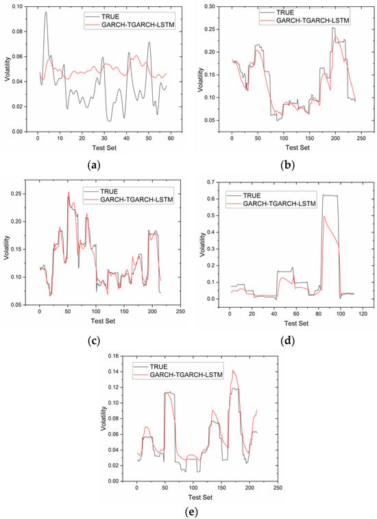
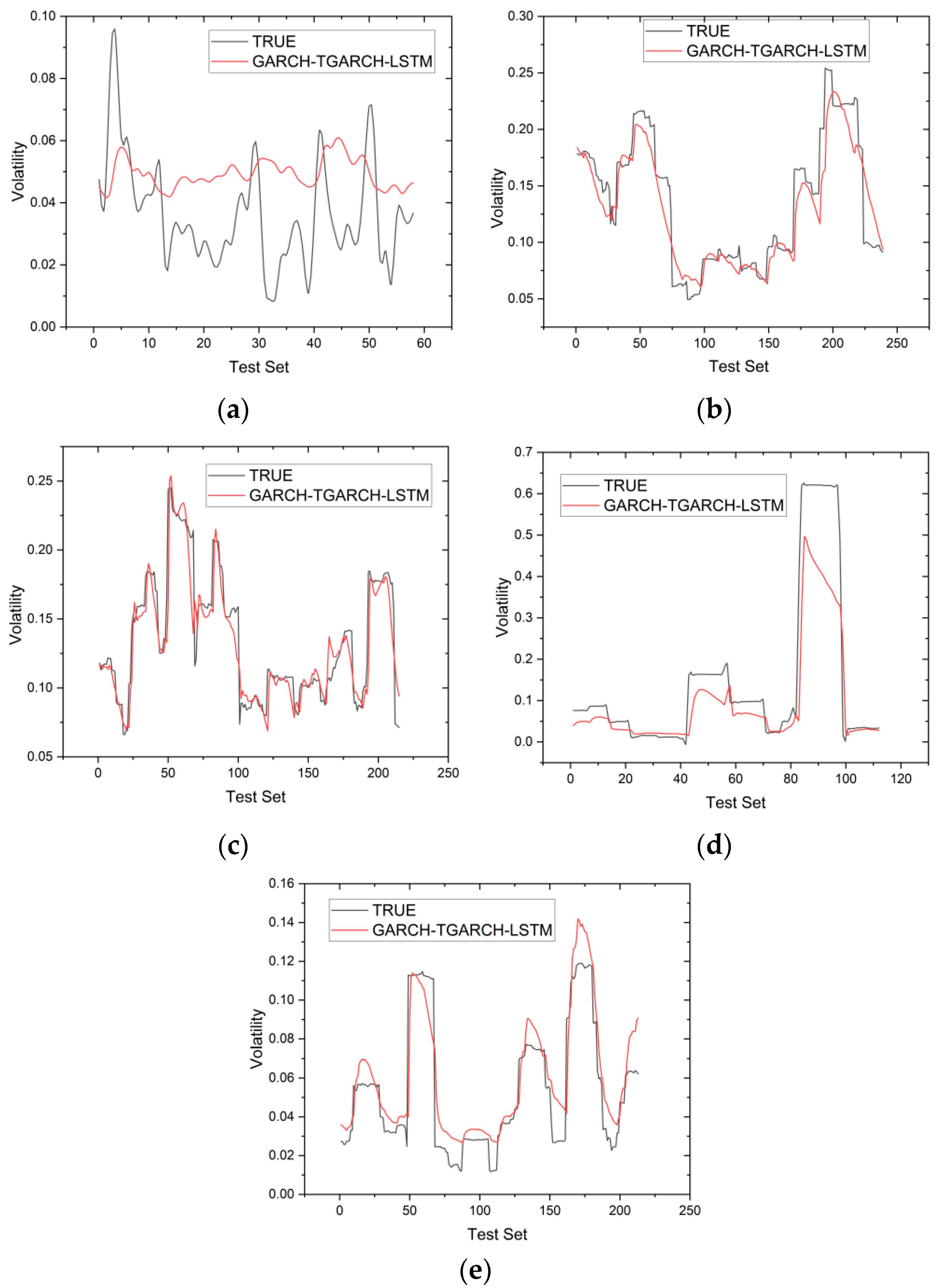
Table 3, Table 4, Table 5, Table 6 and Table 7 report the out-of-sample forecasting performance and the 95% confidence intervals for RMSE of the nine models across the five NFT submarkets. Notably, the GARCH-TGARCH-LSTM model achieves the lowest RMSE among the nine models in all five submarkets. Taking the Atomic market as an example, the GARCH-TGARCH-LSTM model yields an RMSE of 0.02146, representing a reduction of approximately 14% relative to the baseline LSTM model. A similar pattern is observed in the remaining four markets, with RMSE values of 0.02137 (CryptoKitties), 0.01683 (Decentraland), 0.09224 (Gods Unchained), and 0.01415 (OpenSea), corresponding to RMSE reductions of approximately 49%, 13%, 8%, and 29%, respectively, over the baseline LSTM model. The bootstrap confidence intervals provide further insights into the favorable performance ranking of GARCH-TGARCH-LSTM across different NFT submarkets. Figure 2 demonstrates the out-of-sample volatility forecasts of the optimal model among the evaluated specifications (GARCH-TGARCH-LSTM). These results suggest that the combination of GARCH and TGARCH parameters is the best-performing feature set among those tested for the LSTM model in forecasting NFT volatility.

Table 3. Out-of-sample forecasting errors for Atomic.

	RMSE	MSE	MAE	RAE	QLIKE	95% CI (RMSE)
LSTM	0.02495	0.00062	0.02087	0.33089	−4.32618	[0.01981, 0.02999]
GARCH	0.07533	0.00567	0.07138	1.13171	−5.30571	[0.06490, 0.08576]
GARCH-LSTM	0.02320	0.00054	0.01961	0.31090	−5.33687	[0.01870, 0.02781]
TGARCH-LSTM	0.02329	0.00054	0.01976	0.31321	−5.33234	[0.01892, 0.02789]
EGARCH-LSTM	0.02278	0.00052	0.01917	0.30389	−5.33849	[0.01840, 0.02732]
GARCH-TGARCH-LSTM	0.02146	0.00046	0.01830	0.29006	−5.36295	[0.01770, 0.02532]
GARCH-EGARCH-LSTM	0.02310	0.00053	0.01978	0.31366	−5.33020	[0.01908, 0.02736]
TGARCH-EGARCH-LSTM	0.02722	0.00074	0.02415	0.38294	−5.22791	[0.02295, 0.03158]
GARCH-TGARCH-EGARCH-LSTM	0.02340	0.00055	0.02035	0.32259	−5.31638	[0.01962, 0.02738]

Note: Bold values indicate the best forecasting performance among all models.

Table 4. Out-of-sample forecasting errors for CryptoKitties.

	RMSE	MSE	MAE	RAE	QLIKE	95% CI (RMSE)
LSTM	0.04203	0.00177	0.03298	0.61164	−2.99479	[0.02908, 0.05314]
GARCH	0.03837	0.00147	0.03035	0.56283	−2.81821	[0.02671, 0.04839]
GARCH-LSTM	0.02250	0.00051	0.01605	0.29772	−3.12125	[0.01566, 0.02828]
TGARCH-LSTM	0.02217	0.00049	0.01590	0.29477	−3.12430	[0.01487, 0.02822]
EGARCH-LSTM	0.03594	0.00129	0.02620	0.48587	−3.02802	[0.01990, 0.04876]
GARCH-TGARCH-LSTM	0.02137	0.00046	0.01525	0.28273	−3.12610	[0.01492, 0.02679]
GARCH-EGARCH-LSTM	0.02280	0.00052	0.01667	0.30905	−3.12250	[0.01599, 0.02840]
TGARCH-EGARCH-LSTM	0.02371	0.00056	0.01705	0.31618	−3.11397	[0.01561, 0.03008]
GARCH-TGARCH-EGARCH-LSTM	0.02231	0.00050	0.01652	0.30637	−3.12139	[0.01608, 0.02754]

Note: Bold values indicate the best forecasting performance among all models.

Table 5. Out-of-sample forecasting errors for Decentraland.

	RMSE	MSE	MAE	RAE	QLIKE	95% CI (RMSE)
LSTM	0.01930	0.00037	0.01393	0.24211	−2.66879	[0.01520, 0.02285]
GARCH	0.09793	0.00959	0.08310	1.44388	−3.06148	[0.08769, 0.10646]
GARCH-LSTM	0.01749	0.00031	0.01172	0.20366	−3.06990	[0.01375, 0.02106]
TGARCH-LSTM	0.01759	0.00031	0.01087	0.18879	−3.07039	[0.01313, 0.02193]
EGARCH-LSTM	0.01903	0.00036	0.01318	0.22908	−3.06310	[0.01489, 0.02297]
GARCH-TGARCH-LSTM	0.01683	0.00028	0.01033	0.17947	−3.07260	[0.01294, 0.02049]
GARCH-EGARCH-LSTM	0.01754	0.00031	0.01106	0.19225	−3.07014	[0.01349, 0.02150]
TGARCH-EGARCH-LSTM	0.02134	0.00046	0.01603	0.27861	−3.05544	[0.01719, 0.02549]
GARCH-TGARCH-EGARCH-LSTM	0.02215	0.00049	0.01667	0.28956	−3.05292	[0.01733, 0.02680]

Note: Bold values indicate the best forecasting performance among all models.

Table 6. Out-of-sample forecasting errors for Gods Unchained.

	RMSE	MSE	MAE	RAE	QLIKE	95% CI (RMSE)
LSTM	0.10010	0.01002	0.06045	0.53491	0.87137	[0.04272, 0.14961]
GARCH	0.20132	0.04053	0.12017	1.06328	−2.03411	[0.06144, 0.31833]
GARCH-LSTM	0.10763	0.01158	0.06135	0.54288	−2.85778	[0.03446, 0.16768]
TGARCH-LSTM	0.09787	0.00958	0.05600	0.49555	−2.67183	[0.03243, 0.15167]
EGARCH-LSTM	0.10508	0.01104	0.06215	0.54995	−2.18029	[0.04045, 0.15979]
GARCH-TGARCH-LSTM	0.09224	0.00851	0.05322	0.47095	−2.99151	[0.03162, 0.14120]
GARCH-EGARCH-LSTM	0.09467	0.00896	0.05487	0.48547	−2.86794	[0.03410, 0.14463]
TGARCH-EGARCH-LSTM	0.10902	0.01188	0.06277	0.55542	−2.68863	[0.03653, 0.16945]
GARCH-TGARCH-EGARCH-LSTM	0.10456	0.01093	0.05839	0.51666	−2.96495	[0.03188, 0.16299]

Note: Bold values indicate the best forecasting performance among all models.

Table 7. Out-of-sample forecasting errors for OpenSea.

	RMSE	MSE	MAE	RAE	QLIKE	95% CI (RMSE)
LSTM	0.01992	0.00040	0.01646	0.17880	−3.71550	[0.01559, 0.02337]
GARCH	0.09697	0.00940	0.09116	0.99023	−4.98686	[0.08799, 0.10430]
GARCH-LSTM	0.01732	0.00030	0.01455	0.15806	−4.98972	[0.01407, 0.02002]
TGARCH-LSTM	0.01486	0.00022	0.01186	0.12878	−5.02240	[0.01193, 0.01740]
EGARCH-LSTM	0.02501	0.00063	0.02061	0.22389	−4.92935	[0.01973, 0.02920]
GARCH-TGARCH-LSTM	0.01415	0.00020	0.01084	0.11778	−5.03909	[0.01126, 0.01671]
GARCH-EGARCH-LSTM	0.01672	0.00028	0.01431	0.15544	−4.99006	[0.01447, 0.01881]
TGARCH-EGARCH-LSTM	0.01563	0.00024	0.01241	0.13483	−4.99408	[0.01193, 0.01906]
GARCH-TGARCH-EGARCH-LSTM	0.01596	0.00025	0.01296	0.14078	−4.97691	[0.01262, 0.01903]

Note: Bold values indicate the best forecasting performance among all models.

Figure 2. Out-of-sample volatility forecasts of the optimal model among the evaluated specifications (GARCH-TGARCH-LSTM) compared with the observed rolling-window volatility proxy across five NFT submarkets: (a) Atomic; (b) CryptoKitties; (c) Decentraland; (d) Gods Unchained; (e) OpenSea.

4.3.3. DM Test for Comparing Forecast Accuracy

The GARCH-TGARCH-LSTM model serves as the baseline model and is compared with eight other forecasting models across five NFT submarkets. The DM test is based on squared-error loss differentials. For each competing model, the loss difference is defined as the squared prediction error of the competing model minus that of the baseline model. Accordingly, a positive average loss difference indicates that the average squared prediction error of the baseline model is lower. A right-tailed, one-sided alternative hypothesis is adopted to evaluate whether the expected squared prediction loss of the baseline model is lower than that of its competitors. To account for possible heteroscedasticity and autocorrelation in the loss differences, this paper employs the Newey–West heteroscedasticity and autocorrelation consistent (HAC) estimator with Bartlett kernel weights. The truncation lag is determined by a rule that combines the rolling-window length used to construct the volatility proxy with the conventional sample-size-dependent lag rule.

Table 8, Table 9, Table 10, Table 11 and Table 12 report the DM test results comparing each competing model with the GARCH-TGARCH-LSTM model, containing the competing model, DM statistics, p-value, and confidence interval. At the 10% significance level, 35 of the 40 comparisons are statistically significant. Under the specified loss-differential definition, a positive DM statistic indicates that the benchmark model has a lower average squared forecasting loss. Overall, the DM results provide statistical evidence supporting the relative forecasting performance of the GARCH-TGARCH-LSTM model across the five NFT submarkets, although significant differences are not observed in every comparison.

Table 8. DM test results for Atomic.

Competing Model	DM Statistics	p-Value (Right-Tailed)	90% CI (One-Sided)
LSTM	1.97886	0.02392 **	0.00006
GARCH	6.80550	0.00000 ***	0.00423
GARCH-LSTM	1.62800	0.05176 *	0.00002
TGARCH-LSTM	1.95919	0.02505 **	0.00003
EGARCH-LSTM	2.00769	0.02234 **	0.00002
GARCH-EGARCH-LSTM	2.68842	0.00359 ***	0.00004
TGARCH-EGARCH-LSTM	4.24189	0.00001 ***	0.00020
GARCH-TGARCH-EGARCH-LSTM	3.18064	0.00073 ***	0.00005

Note: HAC lag is 3. Asterisks (*, **, ***) in the p-value column denote the statistical significance of the Diebold–Mariano (DM) test, comparing each model’s predictive accuracy against the GARCH-TGARCH-LSTM model. *, **, and *** indicate significance at the 10%, 5%, and 1% levels, respectively.

Table 9. DM test results for CryptoKitties.

Competing Model	DM Statistics	p-Value (Right-Tailed)	90% CI (One-Sided)
LSTM	3.00768	0.00132 ***	0.00075
GARCH	2.90178	0.00186 ***	0.00057
GARCH-LSTM	2.28415	0.01118 **	0.00002
TGARCH-LSTM	1.04880	0.14714	−0.00001
EGARCH-LSTM	2.05548	0.01992 **	0.00031
GARCH-EGARCH-LSTM	1.41843	0.07803 *	0.00001
TGARCH-EGARCH-LSTM	2.11556	0.01719 **	0.00004
GARCH-TGARCH-EGARCH-LSTM	0.92514	0.17745	−0.00002

Note: HAC lag is 29. Asterisks (*, **, ***) in the p-value column denote the statistical significance of the Diebold–Mariano (DM) test, comparing each model’s predictive accuracy against the GARCH-TGARCH-LSTM model. *, **, and *** indicate significance at the 10%, 5%, and 1% levels, respectively.

Table 10. DM test results for Decentraland.

Competing Model	DM Statistics	p-Value (Right-Tailed)	90% CI (One-Sided)
LSTM	2.32242	0.01011 **	0.00004
GARCH	10.56968	0.00000 ***	0.00818
GARCH-LSTM	1.44081	0.07482 *	0.00000
TGARCH-LSTM	0.96154	0.16814	−0.00001
EGARCH-LSTM	2.15046	0.01576 **	0.00003
GARCH-EGARCH-LSTM	1.44927	0.07363 *	0.00000
TGARCH-EGARCH-LSTM	4.16652	0.00002 ***	0.00012
GARCH-TGARCH-EGARCH-LSTM	3.63910	0.00014 ***	0.00013

Note: HAC lag is 18. Asterisks (*, **, ***) in the p-value column denote the statistical significance of the Diebold–Mariano (DM) test, comparing each model’s predictive accuracy against the GARCH-TGARCH-LSTM model. *, **, and *** indicate significance at the 10%, 5%, and 1% levels, respectively.

Table 11. DM test results for Gods Unchained.

Competing Model	DM Statistics	p-Value (Right-Tailed)	90% CI (One-Sided)
LSTM	2.44946	0.00715 ***	0.00072
GARCH	1.50754	0.06584 *	0.00480
GARCH-LSTM	1.39993	0.08077 *	0.00026
TGARCH-LSTM	1.27299	0.10151	−0.00001
EGARCH-LSTM	1.93893	0.02625 **	0.00086
GARCH-EGARCH-LSTM	1.18669	0.11768	−0.00004
TGARCH-EGARCH-LSTM	1.48585	0.06866 *	0.00046
GARCH-TGARCH-EGARCH-LSTM	1.33514	0.09092 *	0.00010

Note: HAC lag is 14. Asterisks (*, **, ***) in the p-value column denote the statistical significance of the Diebold–Mariano (DM) test, comparing each model’s predictive accuracy against the GARCH-TGARCH-LSTM model. *, **, and *** indicate significance at the 10%, 5%, and 1% levels, respectively.

Table 12. DM test results for OpenSea.

Competing Model	DM Statistics	p-Value (Right-Tailed)	90% CI (One-Sided)
LSTM	3.60409	0.00016 ***	0.00013
GARCH	11.64626	0.00000 ***	0.00819
GARCH-LSTM	5.64526	0.00000 ***	0.00008
TGARCH-LSTM	1.91512	0.02774 **	0.00001
EGARCH-LSTM	4.00690	0.00003 ***	0.00029
GARCH-EGARCH-LSTM	5.84025	0.00000 ***	0.00006
TGARCH-EGARCH-LSTM	1.54316	0.06140 *	0.00001
GARCH-TGARCH-EGARCH-LSTM	2.17740	0.01473 **	0.00002

Note: HAC lag is 18. Asterisks (*, **, ***) in the p-value column denote the statistical significance of the Diebold–Mariano (DM) test, comparing each model’s predictive accuracy against the GARCH-TGARCH-LSTM model. *, **, and *** indicate significance at the 10%, 5%, and 1% levels, respectively.

4.3.4. Economic Mechanism Analysis and Discussion

Our study illustrates that the predictive contributions of GARCH-family models depend on the interaction between model structure and the characteristics of the underlying NFT market. Not all combinations of GARCH-type models improve volatility prediction accuracy across the NFT submarkets. We observe that the EGARCH-LSTM model underperforms the TGARCH-LSTM model in the majority of NFT markets, a phenomenon particularly evident in the CryptoKitties and OpenSea markets. This pattern suggests that the threshold-based representation of asymmetric volatility is useful for forecasting in most of the markets considered. One explanation concerns the heterogeneity of NFTs and the discontinuous observation of transaction prices. The heterogeneity of NFTs creates different valuations across market participants and limits the representation of one transaction price of the contemporaneous value of an entire collection. Furthermore, NFT liquidity varies across assets and over time, and changes in market information can affect trading liquidity [48]. Because the observed price series is constructed from completed transactions, changes in buyers’ valuations and sellers’ reservation prices are not reflected immediately in transaction prices. Bargaining and heterogeneous reservation prices further contribute to asymmetric price adjustment. Evidence from NFT pricing research indicates that buyers’ willingness to pay differs from sellers’ willingness to accept and that their price adjustments are asymmetric [49]. These findings suggest that trading outcomes depend not only on changes in underlying valuations but also on negotiation frictions, reservation-price adjustments, and the timing of completed transactions. Differences in the timing and magnitude of price adjustment contribute to asymmetric volatility. From a modeling perspective, the TGARCH model constructs a threshold function, allowing negative shocks (“bad news”) to have an additional effect on conditional variance. Therefore, the TGARCH model possesses higher sensitivity and adaptability when capturing such sudden market fractures and violent price jumps.

Recent literature suggests that the relationship between model complexity and prediction accuracy is not monotonically increasing in financial time series forecasting. For instance, Kim and Won [19] demonstrated that the performance of hybrid models highly depends on the congruence between the underlying GARCH models and data characteristics, rather than merely superimposing additional components. In the context of this NFT study, the standard GARCH parameters effectively extract volatility persistence and clustering over time. Meanwhile, the TGARCH parameters provide additional information on asymmetric volatility responses. This structure is useful when markets experience abrupt repricing with adverse price movements or discontinuous transaction-level adjustments. By contrast, EGARCH models the logarithm of conditional variance and represents asymmetry through a sign-dependent component of standardized shocks. Although this specification can capture asymmetric volatility, its relative forecasting performance depends on how well its functional form matches the observed data. In the present sample, an explicit threshold term better accommodates certain abrupt, asymmetric adjustments in these markets. However, the result does not prove that EGARCH is unsuitable for discontinuous financial data. Differences in effective sample size, volatility proxy construction, and the information contributed by each model component also influence forecasting performance.

Adding more model inputs does not necessarily improve predictive performance, particularly when effective sample sizes are relatively small. Our study reveals that the GARCH-TGARCH-EGARCH-LSTM model underperforms the GARCH-TGARCH-LSTM model across all five NFT submarkets. This suboptimal performance indicates that, when facing an NFT dataset with relatively limited effective sample sizes, the additional feature may introduce noisy signals. The volatility clustering characteristic captured by the GARCH model is complementary to the asymmetric shocks delineated by TGARCH. The former captures volatility persistence, whereas the latter focuses on differences in the effects of positive and negative shocks. The organic combination of these two achieves a useful balance between information content and network model complexity. Under these circumstances, introducing EGARCH logarithmic series provides no substantial marginal effective information. Instead, it increases input redundancy and model complexity, ultimately reducing out-of-sample generalization. These findings highlight the importance of selecting parsimonious input features that reflect the characteristics of the assets being modeled.

Recent studies have also explored alternative neural network structures for financial volatility prediction, including Gated Recurrent Unit (GRU), Bidirectional LSTM (Bi-LSTM), and Convolutional Neural Network–LSTM (CNN-LSTM) models. For instance, Zahid et al. [50] investigated LSTM, GRU, and Bi-LSTM models for Bitcoin volatility forecasting, demonstrating the predictive potential of combining econometric volatility models with recurrent neural network architectures. Similarly, Huang et al. [51] examined the forecasting performance of LSTM and CNN-LSTM models in the Bitcoin market and showed that incorporating convolutional feature extraction could improve short-term volatility forecasts. Compared with these predictive studies, the main contribution of this research lies in identifying the predictive value of combining features extracted from GARCH and TGARCH within an LSTM-based forecasting framework.

5. Concluding Remarks

This study addresses the challenges of volatility prediction in emerging digital asset markets, which arise from pronounced price discontinuities and the absence of traditional market-making mechanisms. By integrating econometric techniques with deep learning approaches, this paper develops and systematically validates a set of hybrid forecasting frameworks. The paper handles millions of transaction records spanning five NFT submarkets and employs data processing techniques to prevent look-ahead bias. Based on multidimensional evaluation metrics (including RMSE, MSE, MAE, RAE, and the QLIKE loss function) and statistical inference (the Diebold–Mariano test), this study reaches the following key conclusions. These findings provide evidence on predictive performance and the potential value of hybrid models for volatility-based risk assessment.

(1)

The hybrid GARCH-TGARCH-LSTM model achieves the lowest out-of-sample RMSE among the nine models evaluated across all five NFT submarkets. Empirical results confirm that this hybrid architecture achieves the best out-of-sample forecasting accuracy across all examined submarkets. Compared to the pure nonlinear benchmark LSTM model, this model achieves improvements ranging from 8% to 49% in RMSE. The DM test provides statistical support for this forecasting advantage. This finding suggests that the integration of various GARCH-type models with LSTM networks can improve volatility forecasting performance in the examined NFT submarkets.

(2)

The incorporation of asymmetric volatility characteristics has heterogeneous effects on the predictive performance of deep learning models. Empirical results reveal that the TGARCH-LSTM model outperforms the EGARCH-LSTM model in four of the five submarkets in terms of forecasting accuracy. This finding suggests that the threshold-based specification of TGARCH is more effective than the logarithmic transformation of EGARCH in capturing asymmetric volatility patterns in the examined NFT submarkets.

(3)

The relationship between model complexity and predictive efficacy is not necessarily monotonic and depends on the alignment between model structure and data characteristics. Empirical evidence demonstrates that the generalization capability of the highest-order hybrid model (GARCH-TGARCH-EGARCH-LSTM) exhibits higher out-of-sample forecasting errors than the simpler GARCH-TGARCH-LSTM model. This finding suggests that adding more volatility input features does not improve forecasting performance when modeling discontinuous NFT price dynamics. Instead, integrating the persistent volatility clustering captured by standard GARCH models with the asymmetric volatility responses identified by TGARCH provides a useful balance between sufficient information extraction and reliable generalization performance.

This study addresses the microstructural characteristics of the NFT market and contributes to the literature on time-series volatility forecasting for NFT assets. Existing NFT-related studies have predominantly focused on identifying cross-sectional pricing factors or analyzing herding behavior within communities. In contrast, this paper examines the forecasting value of incorporating asymmetric GARCH structures to improve time-series volatility forecasting for digital assets. Furthermore, it elucidates how heterogeneous market microstructures affect the applicability of conventional econometric models. This study analyzes the distinctive trading characteristics of the NFT market, including the absence of continuous order books and bargaining-based transactions. It also explains why the threshold segmentation structure of the TGARCH model performs better in the examined samples than the logarithmic smoothing specification of the EGARCH model. These findings provide empirical insights into the selection of econometric models for digital asset volatility. Additionally, this paper shows that incorporating GARCH- and TGARCH-derived conditional variance features as LSTM inputs can improve out-of-sample forecasting performance in the examined NFT submarkets.

The findings of this study also provide practical implications for investors, portfolio managers, and NFT market platforms. For individual investors, volatility forecasts help identify periods of heightened market uncertainty, thereby supporting more informed investment timing and risk management decisions. For portfolio managers, the proposed framework can provide supplementary information for assessing market-specific volatility risks and adjusting portfolio risk exposures. Given the heterogeneous characteristics of NFT submarkets, the forecasting results also highlight the importance of adopting differentiated risk management approaches rather than relying on uniform assumptions across digital assets. For NFT market platforms, volatility forecasting models support the development of market risk monitoring systems, the identification of unusual fluctuations, and the provision of risk-related information to market participants. Nevertheless, forecasting improvements do not necessarily translate into superior investment returns or trading performance, particularly in markets characterized by limited liquidity such as NFT markets.

Despite the development of a hybrid forecasting framework, this study still has certain limitations stemming from inherent data characteristics and modeling choices. These limitations suggest directions for future academic research and methodological improvement: First, the sample period terminates in April 2021, thereby excluding later NFT market regimes, including the NFT boom of late 2021, the collapse in 2022, the crypto winter, and subsequent market restructuring. As researched by Cho et al. [52], NFT trading activities exhibited distinct characteristics during the boom and downturn periods of 2022. Future studies may extend the sample period to cover major market downturns and structural regime shifts and employ formal structural-break analysis to investigate potential changes in volatility dynamics. Second, the proposed forecasting framework primarily draws on GARCH-family models and LSTM networks, omitting more recent forecasting competitors (GRU, CNN-LSTM, Bi-LSTM, etc.). Accordingly, subsequent research could extend the analysis of NFT markets by incorporating alternative recurrent and convolutional neural networks. Third, due to the lack of continuous high-frequency transaction data, this study employs rolling-window standard deviations of log returns as a proxy for volatility. Future research could investigate alternative volatility proxies and assess the sensitivity of model rankings to different volatility measurement approaches.

References

- Borri, N.; Liu, Y.; Tsyvinski, A. The economics of non-fungible tokens. SSRN 2022. [Google Scholar] [CrossRef] [Scilit]
- Vidal Tomás, D. The new crypto niche: NFTs, play-to-earn, and metaverse tokens. Finance Res. Lett. 2022, 47, 102742. [Google Scholar] [CrossRef] [Scilit]
- Kawai, D.; Soska, K.; Routledge, B.; Zetlin-Jones, A.; Christin, N. Anatomy of a digital bubble: Lessons learned from the NFT and metaverse frenzy. arXiv 2025, arXiv:2501.09601. [Google Scholar] [CrossRef] [Scilit]
- Fama, E.F. The behavior of stock-market prices. J. Bus. 1965, 38, 34–105. [Google Scholar] [CrossRef] [Scilit]
- Mandelbrot, B. The variation of some other speculative prices. J. Bus. 1967, 40, 393–413. [Google Scholar] [CrossRef] [Scilit]
- Morgan, I.G. Stock prices and heteroscedasticity. J. Bus. 1976, 49, 496–508. [Google Scholar] [CrossRef] [Scilit]
- Black, F. Studies of stock price volatility changes. In Proceedings of the 1976 Meetings of the Business & Economics Statistics Section; American Statistical Association: Washington, DC, USA, 1976. [Google Scholar]
- Hussain, S.; Chen, J.-H. The return and volatility spillovers among decentralized finance (DeFi) assets. Res. Int. Bus. Finance 2025, 79, 103071. [Google Scholar] [CrossRef] [Scilit]
- Nadini, M.; Alessandretti, L.; Di Giacinto, F.; Martino, M.; Aiello, L.M.; Baronchelli, A. Mapping the NFT revolution: Market trends, trade networks, and visual features. Sci. Rep. 2021, 11, 20902. [Google Scholar] [CrossRef] [Scilit] [PubMed]
- Engle, R.F. Autoregressive conditional heteroscedasticity with estimates of the variance of united kingdom inflation. Econometrica 1982, 50, 987–1007. [Google Scholar] [CrossRef] [Scilit]
- Bollerslev, T. Generalized autoregressive conditional heteroskedasticity. J. Econom. 1986, 31, 307–327. [Google Scholar] [CrossRef] [Scilit]
- Katsiampa, P. Volatility estimation for Bitcoin: A comparison of GARCH models. Econ. Lett. 2017, 158, 3–6. [Google Scholar] [CrossRef] [Scilit]
- Chu, J.; Chan, S.; Nadarajah, S.; Osterrieder, J. GARCH modelling of cryptocurrencies. J. Risk Financ. Manag. 2017, 10, 17. [Google Scholar] [CrossRef] [Scilit]
- Bouri, E.; Azzi, G.; Dyhrberg, A.H. On the return-volatility relationship in the Bitcoin market around the price crash of 2013. Economics 2017, 11, 1–16. [Google Scholar] [CrossRef] [Scilit]
- Hansen, P.R.; Lunde, A. A forecast comparison of volatility models: Does anything beat a GARCH (1, 1). J. Appl. Econom. 2005, 20, 873–889. [Google Scholar] [CrossRef] [Scilit]
- Alberg, D.; Shalit, H.; Yosef, R. Estimating stock market volatility using asymmetric GARCH models. Appl. Financ. Econ. 2008, 18, 1201–1208. [Google Scholar] [CrossRef] [Scilit]
- Di Persio, L.; Honchar, O. Recurrent neural networks approach to the financial forecast of google assets. Int. J. Math. Comput. Simul. 2017, 11, 7–13. [Google Scholar]
- Donaldson, R.G.; Kamstra, M. An artificial neural network-GARCH model for international stock return volatility. J. Empir. Finance 1997, 4, 17–46. [Google Scholar] [CrossRef] [Scilit]
- Kim, H.Y.; Won, C.H. Forecasting the volatility of stock price index: A hybrid model integrating LSTM with multiple GARCH-type models. Expert Syst. Appl. 2018, 103, 25–37. [Google Scholar] [CrossRef] [Scilit]
- Pan, H.; Tang, Y.; Wang, G. A stock index futures price prediction approach based on the MULTI-GARCH-LSTM mixed model. Mathematics 2024, 12, 1677. [Google Scholar] [CrossRef] [Scilit]
- Roh, T.H. Forecasting the volatility of stock price index. Expert Syst. Appl. 2007, 33, 916–922. [Google Scholar] [CrossRef] [Scilit]
- Hu, Y.; Ni, J.; Wen, L. A hybrid deep learning approach by integrating LSTM-ANN networks with GARCH model for copper price volatility prediction. Phys. A 2020, 557, 124907. [Google Scholar] [CrossRef] [Scilit]
- Dai, H.; Huang, G.; Zeng, H.; Zhou, F. Pm2.5 volatility prediction by XGBoost-MLP based on GARCH models. J. Clean. Prod. 2022, 356, 131898. [Google Scholar] [CrossRef] [Scilit]
- Liu, S.; Zhang, Y.; Wang, J.; Feng, D. Fluctuations and Forecasting of Carbon Price Based on A Hybrid Ensemble Learning GARCH-LSTM-Based Approach: A Case of Five Carbon Trading Markets in China. Sustainability 2024, 16, 1588. [Google Scholar] [CrossRef] [Scilit]
- Gao, Z.; He, Y.; Kuruoglu, E.E. A hybrid model integrating LSTM and GARCH for bitcoin price prediction. In Proceedings of the 2021 IEEE 31st International Workshop on Machine Learning for Signal Processing (MLSP), Gold Coast, Australia, 25–28 October 2021. [Google Scholar] [CrossRef] [Scilit]
- Amirshahi, B.; Lahmiri, S. Hybrid deep learning and GARCH-family models for forecasting volatility of cryptocurrencies. Mach. Learn. Appl. 2023, 12, 100465. [Google Scholar] [CrossRef] [Scilit]
- Maouchi, Y.; Charfeddine, L.; El Montasser, G. Understanding digital bubbles amidst the COVID-19 pandemic: Evidence from DeFi and NFTs. Finance Res. Lett. 2022, 47, 102584. [Google Scholar] [CrossRef] [Scilit] [PubMed]
- Schaar, L.; Kampakis, S. Non-fungible tokens as an alternative investment: Evidence from CryptoPunks. J. Br. Blockchain Assoc. 2022, 5, 1–12. [Google Scholar] [CrossRef] [Scilit] [PubMed]
- Horky, F.; Rachel, C.; Fidrmuc, J. Price determinants of non-fungible tokens in the digital art market. Finance Res. Lett. 2022, 48, 103007. [Google Scholar] [CrossRef] [Scilit]
- Nguyen, J.K. Racial discrimination in non-fungible token (NFT) prices? CryptoPunk sales and skin tone. Econ. Lett. 2022, 218, 110727. [Google Scholar] [CrossRef] [Scilit]
- Kang, S.; Oh, H. Decoding the premium: The effect of name fluency on NFT artwork valuation. Econ. Lett. 2025, 255, 112540. [Google Scholar] [CrossRef] [Scilit]
- Bao, T.; Ma, M.; Wen, Y. Herding in the non-fungible token (NFT) market. J. Behav. Exp. Finance 2023, 39, 100837. [Google Scholar] [CrossRef] [Scilit]
- Fridgen, G.; Kräussl, R.; Papageorgiou, O.; Tugnetti, A. Pricing dynamics and herding behaviour of NFTs. Eur. Finance Manag. 2025, 31, 670–710. [Google Scholar] [CrossRef] [Scilit]
- Dowling, M. Is non-fungible token pricing driven by cryptocurrencies? Finance Res. Lett. 2022, 44, 102097. [Google Scholar] [CrossRef] [Scilit]
- Aharon, D.Y.; Demir, E. NFTs and asset class spillovers: Lessons from the period around the COVID-19 pandemic. Finance Res. Lett. 2022, 47, 102515. [Google Scholar] [CrossRef] [Scilit] [PubMed]
- Umar, Z.; Alwahedi, W.; Zaremba, A.; Vo, X.V. Return and volatility connectedness of the non-fungible tokens segments. J. Behav. Exp. Finance 2022, 35, 100692. [Google Scholar] [CrossRef] [Scilit]
- Yousaf, I.; Yarovaya, L. Static and dynamic connectedness between NFTs, Defi and other assets: Portfolio implication. Glob. Finance J. 2022, 53, 100719. [Google Scholar] [CrossRef] [Scilit]
- Glosten, L.R.; Jagannathan, R.; Runkle, D.E. On the relation between the expected value and the volatility of the nominal excess return on stocks. J. Finance 1993, 48, 1779–1801. [Google Scholar] [CrossRef]
- Nelson, D.B. Conditional heteroskedasticity in asset returns: A new approach. Econometrica 1991, 59, 347–370. [Google Scholar] [CrossRef] [Scilit]
- LeCun, Y.; Bengio, Y.; Hinton, G. Deep learning. Nature 2015, 521, 436–444. [Google Scholar] [CrossRef] [Scilit] [PubMed]
- Hochreiter, S.; Schmidhuber, J. Long short-term memory. Neural Comput. 1997, 9, 1735–1780. [Google Scholar] [CrossRef] [Scilit] [PubMed]
- Shu, Q.; Xiong, H.; Jiang, W.; Mamon, R. A novel perspective on forecasting non-ferrous metals’ volatility: Integrating deep learning techniques with econometric models. Finance Res. Lett. 2023, 58, 104482. [Google Scholar] [CrossRef] [Scilit]
- Brownlees, C.T.; Gallo, G.M. Comparison of Volatility Measures: A Risk Management Perspective. J. Financ. Econom. 2010, 8, 29–56. [Google Scholar] [CrossRef] [Scilit]
- Patton, A.J. Volatility forecast comparison using imperfect volatility proxies. J. Econom. 2011, 160, 246–256. [Google Scholar] [CrossRef] [Scilit]
- Diebold, F.X.; Mariano, R.S. Comparing Predictive Accuracy. J. Bus. Econ. Stat. 1995, 13, 253–263. [Google Scholar] [CrossRef] [Scilit]
- Snoek, J.; Larochelle, H.; Adams, R.P. Practical Bayesian Optimization of Machine Learning Algorithms. In Advances in Neural Information Processing Systems 25; Curran Associates: Red Hook, NY, USA, 2012; pp. 2951–2959. [Google Scholar]
- Kingma, D.P.; Ba, J. Adam: A Method for Stochastic Optimization. arXiv 2014, arXiv:1412.6980. [Google Scholar] [CrossRef] [Scilit]
- Wilkoff, S.; Yildiz, S. The behavior and determinants of illiquidity in the non-fungible tokens (NFTs) market. Glob. Finance J. 2023, 55, 100782. [Google Scholar] [CrossRef] [Scilit]
- Liu, Y.; Huangfu, B.; Qiao, Z.; Zhao, X. Rarity, the WTA-WTP disparity, and price adjustments in the NFT market. Int. J. Res. Mark. 2025, 42, 594–609. [Google Scholar] [CrossRef] [Scilit]
- Zahid, M.; Iqbal, F.; Koutmos, D. Forecasting Bitcoin Volatility Using Hybrid GARCH Models with Machine Learning. Risks 2022, 10, 237. [Google Scholar] [CrossRef] [Scilit]
- Huang, Z.-C.; Sangiorgi, I.; Urquhart, A. Forecasting Bitcoin volatility using machine learning techniques. J. Int. Financ. Mark. Inst. Money 2024, 97, 102064. [Google Scholar] [CrossRef] [Scilit]
- Cho, E.; Jensen, G.; Yoo, Y.; Mahanti, A.; Kim, J.-K. Characterizing the Initial and Subsequent NFT Sales Market Dynamics: Perspectives from Boom and Slump Periods. IEEE Access 2024, 12, 3638–3658. [Google Scholar] [CrossRef] [Scilit]
Disclaimer/Publisher’s Note: The statements, opinions and data contained in all publications are solely those of the individual author(s) and contributor(s) and not of MDPI and/or the editor(s). MDPI and/or the editor(s) disclaim responsibility for any injury to people or property resulting from any ideas, methods, instructions or products referred to in the content. |
© 2026 by the authors. Licensee MDPI, Basel, Switzerland. This article is an open access article distributed under the terms and conditions of the Creative Commons Attribution (CC BY) license.