


Abstract
The Marshall–Olkin bivariate Weibull model with modified singularity assigns positive probability to an unknown ray . We study inference for its location under exact and finite-resolution observation. With exact observations, repeated common-shock ratios permit support recovery, and conditional profiling reduces the rate-parameter optimization. With grouped observations, a rectangle likelihood retains continuous and singular mass, and a breakpoint-aware search accommodates the piecewise-smooth likelihood. In simulations with 1000 replications per scenario, the ratio of mean RMSE across four recording resolutions, comparing midpoint substitution with interval-aware estimation of , was approximately 29 and 39 for common-shock probabilities 0.30 and 0.50. At probability 0.10 and the coarsest resolution, 24.4% of replications met an operational weak-information criterion. A direct comparison also shows lower rate-parameter RMSE for interval-aware estimation at moderate and large singular masses, whereas shape-parameter accuracy is similar and not uniformly better. Hessian-based intervals were unavailable in many replications and their conditional coverage could be below nominal. An exploratory computational illustration with two river-response episodes demonstrates the calculations and sensitivity without supporting substantive hydrological conclusions. The study clarifies how finite recording resolution changes inference on a moving singular support and limits local uncertainty summaries.
Keywords:
Marshall–Olkin bivariate Weibull; singular distribution; rounded data; grouped observations; maximum likelihood; profile likelihood; weak identification; common-shock model MSC:
62H12; 62F10; 62F12; 62E15
1. Introduction
Multivariate lifetime models based on latent shocks occupy a distinctive place in reliability and survival analysis because they connect a probabilistic dependence mechanism with an explicit stochastic construction. The seminal Marshall–Olkin model represents each component lifetime as the minimum of an idiosyncratic shock and one or more shared shocks, thereby generating dependence through physically interpretable failure mechanisms rather than through an arbitrary association parameter [1,2,3,4]. In the bivariate case, this construction produces an unusual probability law: part of the distribution is absolutely continuous on two open regions of , while a positive amount of probability is concentrated on a one-dimensional set. This singular–continuous mixture distinguishes Marshall–Olkin models from ordinary smooth bivariate families and is central to their interpretation in common-cause failure, dependent competing risks, systemic risk, and multivariate reliability [5,6,7,8,9]. The same singular structure is also responsible for several nonstandard inferential features, because the common-shock mechanism is represented geometrically by a support set of lower dimension.
Estimation and hypothesis testing for the bivariate exponential distribution have been studied previously [10]. Replacing exponential margins by Weibull margins substantially enlarges the range of lifetime shapes while preserving the shock interpretation. The resulting Marshall–Olkin bivariate Weibull (MOBW) distribution allows monotone nonconstant hazards and has therefore attracted a broad inferential literature. Maximum-likelihood estimation is analytically difficult because the model combines singular and absolutely continuous components; EM-type methods were developed for multivariate shock models and subsequently specialized to the MOBW family [11,12]. Bayesian estimation, importance sampling, and alternative likelihood procedures have also been studied [13,14]. A parallel line of work has incorporated censoring, progressive censoring, interval observation, accelerated life testing, and dependent competing risks [15,16,17,18,19,20]. These contributions demonstrate that the MOBW model is inferentially useful but numerically delicate, especially when information about the shock component is incomplete. Related bivariate Weibull regression and shock-model developments further emphasize the importance of retaining the mechanistic interpretation of dependence [21,22].
The Marshall–Olkin bivariate Weibull model with modified singularity (MOBW-) was introduced to relax a structural restriction of the classical model: the common-shock mass need not lie on the diagonal [23]. In MOBW-, the singular component is supported on
so that controls the geometric position of the common-shock line. The classical MOBW model is recovered at . Previous work established the distributional properties, marginal laws, hazard quantities, survival copula, and dependence characteristics of this construction [23]. What remains substantially less developed is statistical inference for itself. This is not merely an additional smooth scale or shape parameter: varying moves a singular support and simultaneously changes the second marginal through . Consequently, information about arises from two different sources—the geometry of the singular component and the smooth marginal/joint probabilities—whose relative importance changes dramatically with the amount of common-shock mass.
This feature places the inferential problem close to the broader class of nonregular likelihood problems in which standard differentiability and fixed-support arguments cannot be applied mechanically. Classical likelihood theory typically relies on a parameter-independent support and a locally quadratic log-likelihood. When a parameter changes the support, or when the information matrix becomes nearly singular, maximum-likelihood estimators may exhibit nonstandard rates, non-Gaussian limits, unstable curvature, or poor Wald approximations [24,25,26,27]. The present model has its own specific geometry, so general nonregular results do not transfer verbatim; nevertheless, they provide the appropriate inferential perspective. In particular, a Hessian-based standard error can be reliable only when the selected optimum lies in a locally smooth region with sufficient curvature. Profile likelihood is therefore especially attractive because it evaluates evidence for after re-optimizing the nuisance parameters rather than relying entirely on a quadratic approximation at a single point [28,29,30,31].
A second layer of nonregularity is introduced by finite recording resolution. In practice, continuous lifetimes, concentrations, distances, or machine-recorded durations are frequently rounded, grouped, heaped, or digitized. The resulting observation is not an exact point but a set known to contain the latent value. The coarse-data framework of Heitjan and Rubin [32] provides a general formulation encompassing rounding, grouping, censoring, and partial categorization; when the grouping mechanism is fixed or ignorable, likelihood inference should be based on the probability assigned to the observed set [33,34]. The inferential consequences of ignoring rounding have long been recognized [35], and modern work has shown that direct likelihood treatment of rounded observations can materially differ from analyses that simply replace intervals by representative points [36,37].
The interaction between rounding and singularity is particularly consequential. An exact common-shock observation satisfies and therefore reveals the ratio without measurement error. After rounding, however, the observed datum is a rectangle:
which may intersect for a range of values of . The discrete record no longer identifies the singular ratio exactly. Moreover, midpoint substitution may create repeated pseudo-ratios that were not present in the latent sample or may move a genuinely singular observation away from the correct support. Thus, a method that treats rectangle midpoints as exact data changes the geometry of the statistical model, whereas a rectangle likelihood preserves the probability assigned by both the absolutely continuous and singular components. This distinction is central to the present paper.
The inferential questions addressed here can therefore be stated explicitly. First, under exact observation, how can the singular location be recovered and how does its recovery probability depend on the common-shock mass and sample size? Second, conditional on , can the regular rate parameters be profiled analytically to be sufficient in reducing the numerical dimension of the exact-data likelihood? Third, under a finite resolution, how should the likelihood be constructed so that the singular mass inside each observation rectangle is retained automatically? Fourth, because the rounded likelihood is only piecewise smooth in , how can one search globally without enumerating an excessive number of smooth regions? Finally, when the singular mass is small, how can weak information on be distinguished from mere optimizer failure?
The MOBW- distribution itself was introduced by Brango et al. [23]; it is not a new distribution in the present paper. Our contribution is an inferential framework for its unknown singular-line location: conditional rate profiling, exact support recovery, a characterization of recording-induced breakpoints, and finite-sample profile diagnostics. The rectangle identity is standard inclusion–exclusion, not a new probability identity. Bai et al. [17] study the classical three-shock MOBW model under progressive interval censoring; their observation scheme includes inspection and withdrawal information. Here, each observation is a known bivariate recording rectangle and the singular ray has an unknown location . Li, Sun, and Song [38] develop graphical and marginal procedures for bivariate right-censored failure times, rather than the fixed-grid recording scheme used here. These studies motivate the likelihood treatment of incomplete observations, but they do not supply the present moving-ray breakpoint search. Unlike the distributional study [23], we investigate how the observation mechanism changes estimation and uncertainty for .
The paper is organized as follows. Section 2 develops the stochastic representation, mixture geometry, exact likelihood, conditional profiling equations, exact support recovery, rectangle likelihood, posterior common-shock probabilities, uncertainty quantification, and the hybrid profile algorithm. Section 3 reports the exact and rounded-data Monte Carlo results. Section 4 presents an exploratory joint analysis of asynchronous river-response times, including singular-probability maps, profile likelihood and sensitivity diagnostics. Section 5 relates the findings to the existing Marshall–Olkin and coarse-data literature and discusses the weak-information regime. Section 6 concludes the study.
2. Materials and Methods
2.1. MOBW- Shock Representation
Let be independent exponential random variables with rates , let , and let . Define
and , . Then,
where . The marginal survival functions are
The model has positive mass on and
For simulation design,
The absolutely continuous density has two pieces. For ,
and for ,
Along , using x as the one-dimensional coordinate,
2.2. Mixture Geometry and Inferential Parameterization
Let and . The three mechanism probabilities are
Thus, the law can be viewed as a singular–continuous mixture, with the components supported on , , and , respectively. This representation is used to clarify the inferential geometry rather than as a computational mixture likelihood. The parameter has a dual role: it moves the singular ray and enters the second marginal through . The log-scale parameter is useful numerically because and the classical MOBW model corresponds to .
Remark 1 (Moving-support nonregularity).
For exact observations, changing μ changes both the partition into the two continuous regions and the support of the singular component. Hence, ordinary fixed-support regularity conditions do not hold automatically. Model-specific analysis and profile diagnostics are therefore preferable to the mechanical application of regular likelihood approximations [24,25].
2.3. Exact-Observation Likelihood and Conditional Profiling
For fixed , classify observations into , , and , with counts . Define
For fixed , use the dominating measure obtained by adding planar Lebesgue measure on the two open regions and the pushforward of by on the ray. The singular density is therefore expressed in the x coordinate, not in arc length. Relative to this fixed- measure, the exact log-likelihood is
The score equations for the rate parameters are
For fixed and , the rate log-likelihood is strictly concave: its Hessian contains and additional negative semidefinite terms. It tends to at a rate boundary and as the rate vector diverges, since all exposure sums are positive. Thus, an interior maximizer exists and is unique. When a component count vanishes, this interior argument cannot be used; constrained boundary fitting is required.
Proposition 1 (Conditional profiling of the rate parameters).
Fix and , and let and . For an interior solution with , conditional on , the score equations for and are equivalent to
Each equation has a unique positive root. Substitution of these roots into reduces the three-dimensional rate problem to the scalar equation
Proof.
Multiplying Equations (16) and (17) by their positive denominators yields the quadratics. In both cases, the leading coefficient is positive and the constant term is negative, so the two roots have opposite signs and exactly one is positive. Substitution into Equation (18) gives Equation (21). The Hessian of the rate log-likelihood is negative definite under the stated positive-count assumptions; its Schur complement shows that the profiled score is strictly decreasing. The unique interior maximum therefore gives the unique zero of that score. □
For numerical stability, the positive quadratic root is evaluated in cancellation-resistant form. For each candidate , Equation (21) is bracketed and solved numerically, yielding . The resulting profile is maximized over . Boundary cases, including samples with zero component counts, are handled by constrained optimization rather than forcing the interior equations.
The conditional exact likelihood does not define an ordinary density comparison across arbitrary values with different singular supports. Exact estimation first uses repeated ratios to recover the support and then fits the remaining parameters conditionally. If fewer than two common-shock observations are present, the repeated-ratio rule has no guaranteed recovery; Proposition 2 is a sufficient recovery result, not a claim of uniqueness for every finite sample.
2.4. Computational Verification
The profiling equations are algebraic quadratic equations, not recurrence relations. Their reduction in dimension alone does not imply a measured speedup. We therefore compare the conditional scalar-root calculation with direct joint optimization of three rates at fixed , and independently verify rectangle probabilities by numerical integration:
where the last integral is zero when . Planar quadrature alone misses singular mass. The numerical benchmark and its limited scope are reported in Section 3.7; the R script (version 4.2.2 Patched), case-level errors, timings and session information accompany this revision.
2.5. Exact Recovery of the Singularity Parameter
Proposition 2 (Exact support recovery).
Assume an independent identically distributed sample with and mathematically exact observations. If at least two observations arise from the common-shock component, then μ is recovered almost surely as the unique repeated value of the ratios . If denotes the number of common-shock observations in a sample of size n, then
Proof.
A common-shock observation satisfies . Conditional on either absolutely continuous region, has a continuous distribution, so repeated continuous-component ratios, as well as the equality of a continuous-component ratio with , have a probability of zero. Since , Equation (23) follows. □
2.6. Finite-Resolution Observations and Rectangle Likelihood
For a fixed, known recording grid (or an ignorable grouping mechanism), suppose the latent pair is recorded only through . Its probability is
and
For each rectangle, analytic branches can change only at finite corner ratios. Let be the set of positive finite values among , , , and across observations.
Proposition 3 (Piecewise smoothness of the rounded likelihood).
Assume for all observed rectangles. Conditional on , the function is continuous on and infinitely differentiable on each connected component of .
Proof.
At a fixed corner with , is continuous in and has a fixed branch on any interval not containing . Therefore, every survival term is smooth between consecutive breakpoints and continuous at a breakpoint. For , the corner term is constant in ; for , its branch is fixed for . The corner contributes the constant one. Finite linear combinations preserve continuity, and when , the logarithm preserves smoothness inside each open region. □
This finite-breakpoint structure explains why a global search over is needed while smooth optimization remains appropriate inside each region. Equation (24) automatically includes both continuous and singular probability; no ad hoc classification of a rounded observation as singular or non-singular is required. In simulation, a common grid width is used, where are the generating marginal medians and r is the relative recording resolution.
2.7. Posterior Common-Shock Membership
Let , , and . If , integration of the singular density gives
with otherwise. Hence,
is the model-based conditional probability of common-shock membership given the recorded rectangle. A positive-length intersection contributes its integrated mass; a contact at a single corner contributes zero because the coordinate along the ray is continuously distributed. When all endpoints are positive, such an intersection occurs exactly for . At zero endpoints, the max/min definition remains valid without dividing by zero. In simulation, classification accuracy is summarized by the Brier score , where is the simulated component indicator.
2.8. Hybrid Profile Optimization for Rounded Data
Define
and . The implemented estimator uses a hybrid profile-search strategy over finite computational bounds. It returns the best candidate found and is not a certificate of a global maximum. A coarse grid on is evaluated with data-adaptive landmarks and nearby observed breakpoints. Several well-separated high-likelihood points are retained, the full five-parameter vector is jointly refined in neighboring smooth regions, non-smooth breakpoints are evaluated explicitly, and the best candidate receives a final conditional refit. For a candidate ,
is used diagnostically. Routine calibration is not asserted near a non-smooth breakpoint or in weak-information samples [28,29,31].
Table 1 summarizes the numerical settings used for simulation fitting.
Table 1.
Simulation settings audited from the frozen v2.4.2 R engine. These are distinct from the river-illustration bounds.
The implementation compresses duplicate rectangles and evaluates the four survival terms vectorially. It rejects nonfinite probabilities and values below ; other nonpositive results are floored at the smallest positive normalized double. This flooring prevents undefined logarithms but does not cure cancellation or certify relative accuracy. Tiny or tail probabilities should be checked with independent integration or higher-precision arithmetic. The benchmark includes such cases.
For local uncertainty, the frozen engine does not test whether the entire numerical differentiation stencil stays inside one smooth region, nor does it test stability under alternative step sizes. A positive-definite numerical Hessian is consequently only a working diagnostic. We retain the original uncertainty results with this limitation rather than claiming a stricter criterion was used. Smoothness for fixed nuisance parameters also does not guarantee smoothness of a profiled envelope when its maximizing branch changes.
2.9. Local Likelihood Geometry in Smooth Rounded-Data Regions
Let and . Away from breakpoints,
and the observed information is
Proposition 4 (Local quadratic representation).
Suppose is an interior stationary point, all observed rectangles have positive probability in a neighborhood of , is separated from the breakpoint set, and is positive definite. Then, for within that smooth region,
Proof.
Piecewise smoothness provides a twice continuously differentiable neighborhood. A second-order Taylor expansion around the stationary point eliminates the first-order term and Equation (31) supplies the quadratic term. □
Numerical curvature is computed on . If is positive definite, the working covariance on the original scale is , with . In the implemented calculation, no Wald standard error is returned when is at a breakpoint or curvature is unreliable.
This proposition is a deterministic local Taylor expansion, not a proof of asymptotic normality or nominal Wald coverage for a moving-support model. In particular, breakpoint proximity, boundary solutions and weak information can invalidate a routine quadratic interpretation.
2.10. Operational Weak-Identification Diagnostic and Midpoint Comparator
Let and
A replication is flagged as weakly identified if either or there is a well-separated secondary local maximum within 2 log-likelihood units of the global maximum, with . This is an operational finite-sample diagnostic, not a new asymptotic definition of weak identification [26,27,30,31,39].
The midpoint comparator replaces each rectangle by its center and applies the exact-data procedure to these pseudo-observations. Ratios are sorted and clustered by , comparing each new ratio with the first member of its cluster. Among clusters of size at least two, only those with largest multiplicity are retained. Their mean ratios are candidate slopes. Each candidate is conditionally fitted and the largest conditional objective is selected; an exact objective tie selects the first candidate in ascending ratio order. With no repeated ratio or no finite candidate fit, the comparator returns a failure. This is the specific heuristic studied, not every possible midpoint procedure. Comparisons of conditional objectives at different rays are part of this heuristic, not an ordinary common-measure exact likelihood for unknown . Artificial repeated midpoint ratios explain why its behavior differs from Proposition 2.
In practical terms, weak information means that materially different slopes remain compatible after nuisance reoptimization. At , the model reduces to and is independent of . A small positive alone does not prove weak information; sample size, resolution and observed geometry matter. Applied diagnostics should report the full profile, competing modes, contact with search bounds, fitted singular mass, and sensitivity to starts and defensible observation definitions. The chi-square likelihood drop defines an operational support set, not a confidence set with established coverage here. The stored width and competing-mode flags approximate this set on evaluated profile points and are sensitive to search resolution.
2.11. Monte Carlo Design
The final reporting set uses replications per scenario and seed 28082026. A common reference configuration is
with determined by Equation (5). The exact benchmark contains 17 distinct scenarios varying , , , , and , with duplicate reference configurations removed. The rounded study uses and varies and shock balance.
For each replication, the code draws independent , equivalently for independent uniform variables, and sets
The common-shock label is . The known generating medians are and . For , the recording rule is , and
The grid origin is zero. Here, “rounding” means fixed-width interval recording, not rounding to the nearest multiple. Both methods are fitted to the same recorded sample. No failed run is replaced. For a parameter and B finite estimates indexed by V, the summaries are
Mean squared error is . Empirical SD uses divisor . Mean model-based SE averages available positive finite SEs and is not the empirical SD. Conditional coverage averages only over estimates with available SE; the effective denominator is reported. In particular, the original midpoint regular-parameter intervals are conditional on its selected slope and do not propagate slope-selection uncertainty. Main-design point estimates are available for all 1000 replications for both methods. Supplementary comparisons report bias, RMSE, SE availability and coverage denominators for each parameter and method.
For each estimator and parameter, performance is summarized using bias, RMSE, empirical standard deviation, mean model-based standard error when available, empirical 95% Wald coverage, Brier score, fit success, and weak-identification frequency. For , Wald coverage is reported only among replications for which the observed information matrix on the log-parameter scale was positive definite and yielded a finite Hessian-based standard error. The denominator shown explicitly is therefore the number of such replications, rather than the full runs. These conditional coverages describe local quadratic inference when available and should not be interpreted as unconditional frequentist coverage of the estimator. Scenarios initially computed with 2000 replications were standardized to their first 1000 replications in the final reporting set; the source simulation objects were preserved unchanged.
3. Results
3.1. Exact-Observation Benchmark
Table 2 reports the full exact benchmark. The conditional likelihood routine returned a finite fit in every replication of all 17 scenarios. Support recovery also succeeded in every reported replication, consistent with the theoretical recovery probability in Equation (23), which is essentially one for the selected combinations of n and .
Table 2.
Exact-observation benchmark over the 17 Monte Carlo scenarios. Entries for , , , and are RMSE (empirical coverage of the nominal 95% Wald interval). The last columns give RMSE() and empirical recovery probability of . All values use replications.
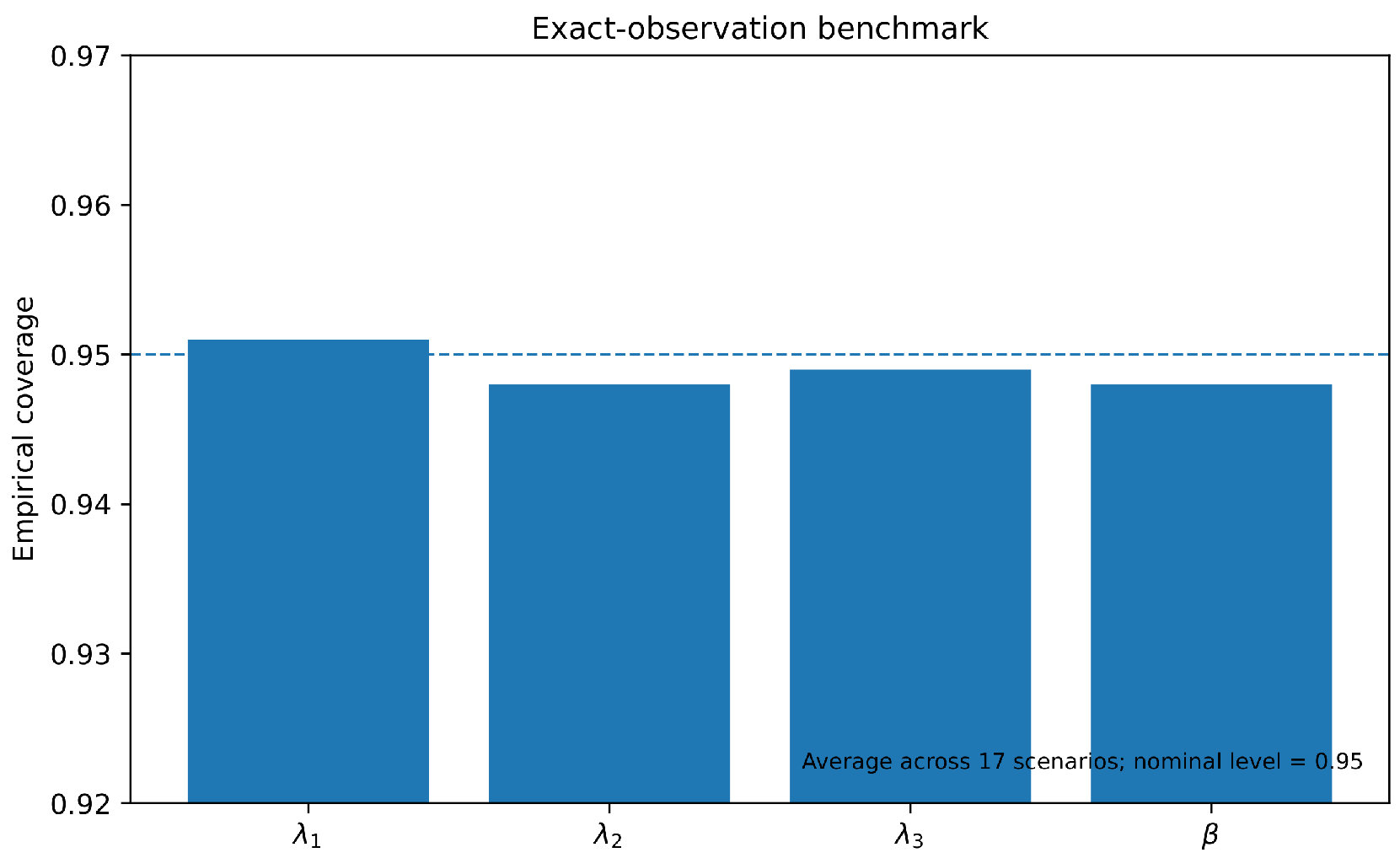
The regular parameters displayed stable frequentist behavior. Averaged across the 17 scenarios, empirical 95% coverage was 0.951 for , 0.948 for , 0.949 for , and 0.948 for . Scenario-specific ranges were , , , and , respectively. RMSE decreased with sample size, while varying , , , or the balance between and did not destabilize fitting.
Figure 1 summarizes average coverage across the exact-observation scenarios.
Figure 1.
Average empirical coverage of nominal 95% Wald intervals for regular parameters in the exact-observation benchmark. The horizontal line denotes the nominal value 0.95.
3.2. Estimation of Under Finite Recording Resolution
The principal rounded-data comparison uses , , , and , so the generating singularity parameter is . When singular mass is moderate or large, the interval-aware estimator is markedly more accurate than midpoint substitution. For , its mean RMSE across the four resolutions is 0.00506, compared with 0.14714 for the naive estimator, a ratio of approximately 29.1. For , the corresponding values are 0.00295 and 0.11494, with a ratio of approximately 39.0. At , RMSE increases from 0.00083 at to 0.01188 at , whereas the naive RMSE rises from 0.07917 to 0.18127.
Figure 2.
RMSE of versus recording resolution, comparing interval-aware maximum likelihood and midpoint substitution.
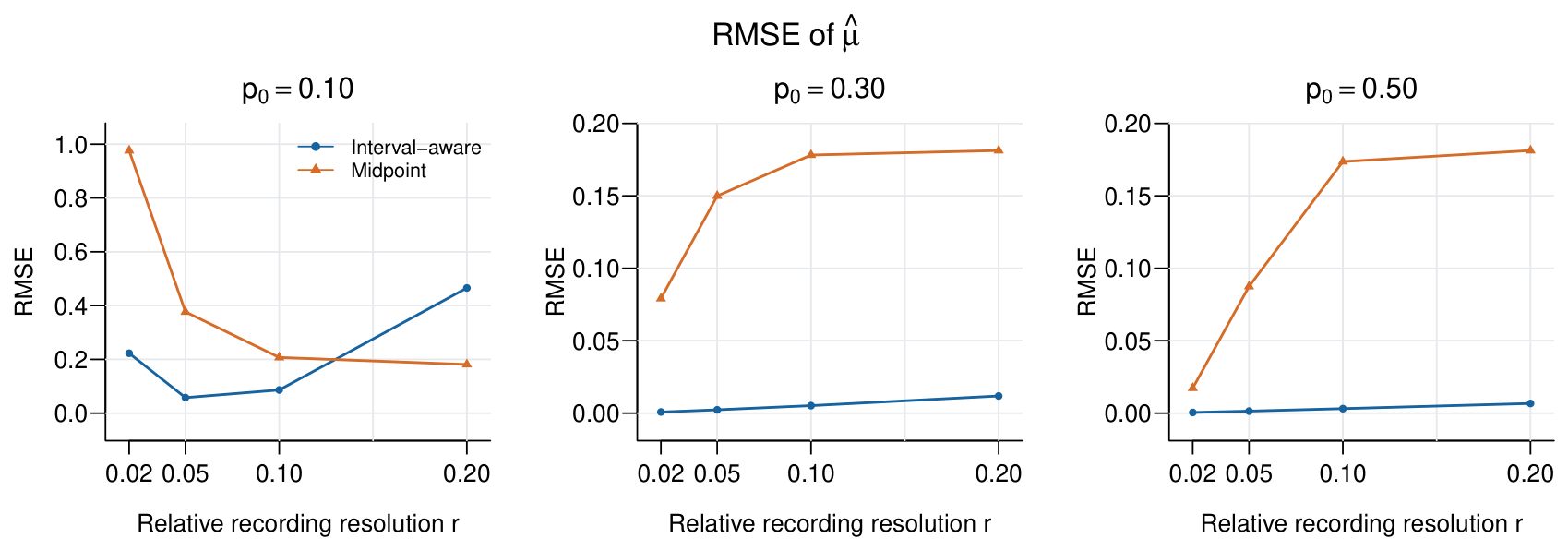
Figure 3.
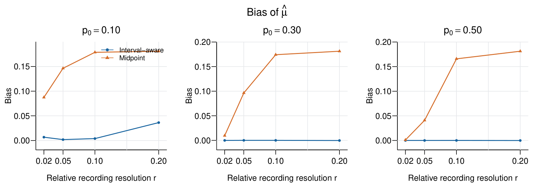
Bias of versus recording resolution.
3.3. Weak Identification When Singular Mass Is Small
The main departure from stable behavior occurs at . The weak-identification rate increases from 0.2% at to 0.3% at , 5.0% at , and 24.4% at . In the most challenging configuration, , overall RMSE of is 0.466. This error is concentrated in weakly identified samples: RMSE is approximately 0.0497 among non-weak replications and 0.938 among weak replications. At only 0.2% of replications are weakly identified; overall RMSE is 0.223 but RMSE among non-weak replications is only 0.0042. These results distinguish inferential information from numerical convergence: a numerical fit can be returned while the data contain little information about the moving singular support.
Figure 4 displays the weak-identification frequencies.
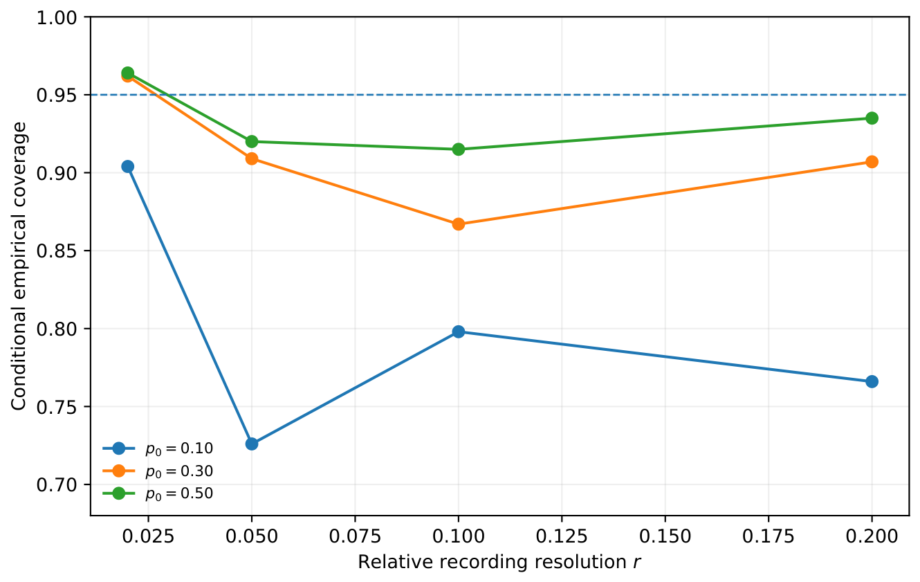
Wald inference for shows the same limitation. Average conditional coverage across the four resolutions is approximately 0.798, 0.911, and 0.934 for , , and , respectively. These coverages are computed only among replications with a finite Hessian-based standard error; the corresponding denominators, reported in Table 3, range from 288 to 837 out of the replications. They therefore summarize local Wald inference when available and should not be interpreted as unconditional frequentist coverage of the estimator.
Figure 4.
Empirical weak-identification rate for as a function of recording resolution and singular mass. The orange () and green () series coincide at zero; the green series overlays the orange series.
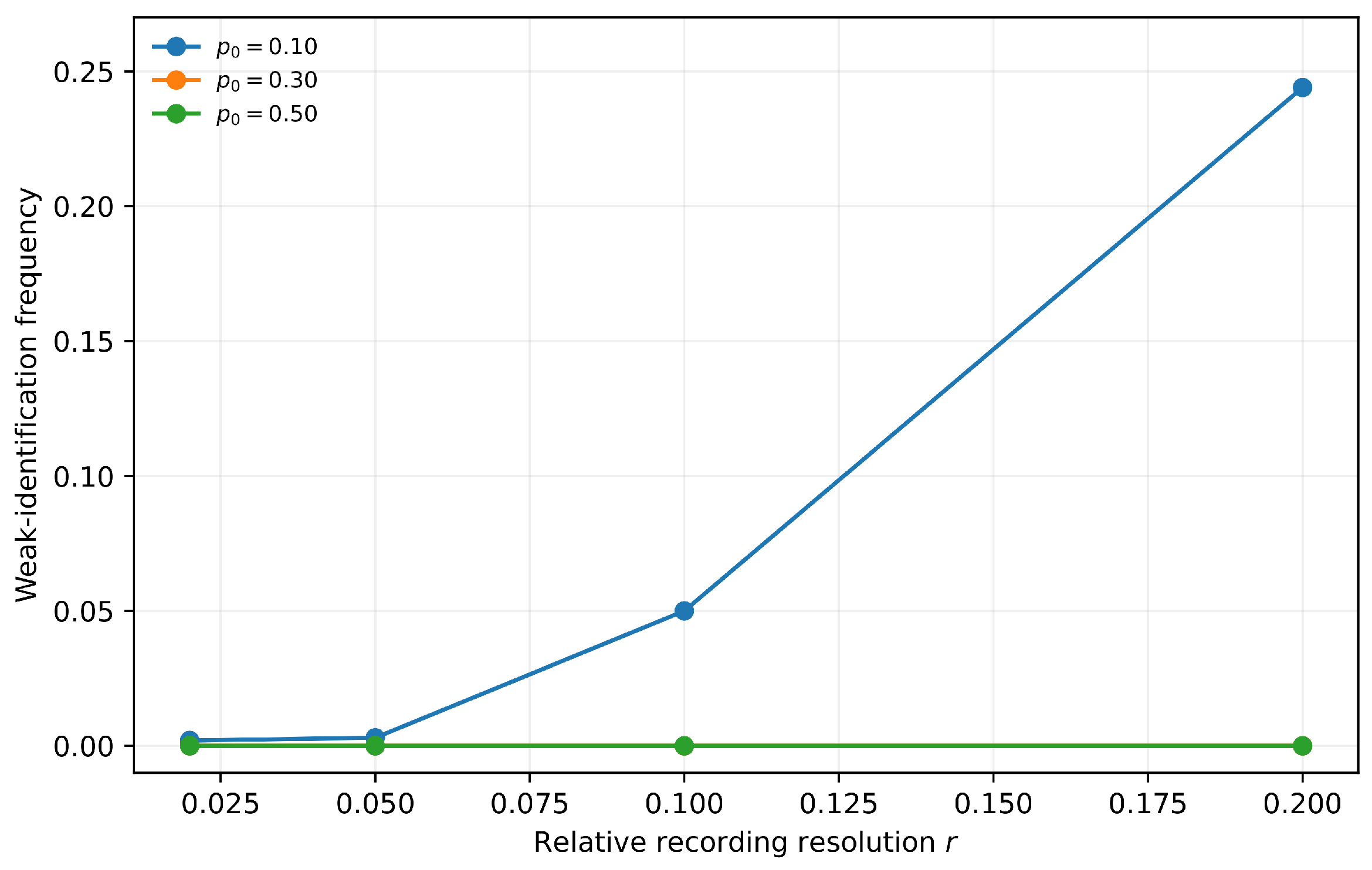
Table 3.
Detailed performance for in the main rounded-data design. Coverage is conditional on a finite Hessian-based standard error obtained with the frozen numerical-curvature rule; the denominator in parentheses is the number of eligible replications and is therefore not necessarily . Weak ID is the empirical weak-identification rate and Brier is the mean Brier score.
Figure 5 shows conditional coverage across recording resolutions.
Figure 5.
Conditional empirical coverage of nominal 95% Wald intervals for under the interval-aware estimator, computed only among replications with a finite Hessian-based standard error. The horizontal dashed line marks nominal coverage 0.95.
3.4. Common-Shock Classification
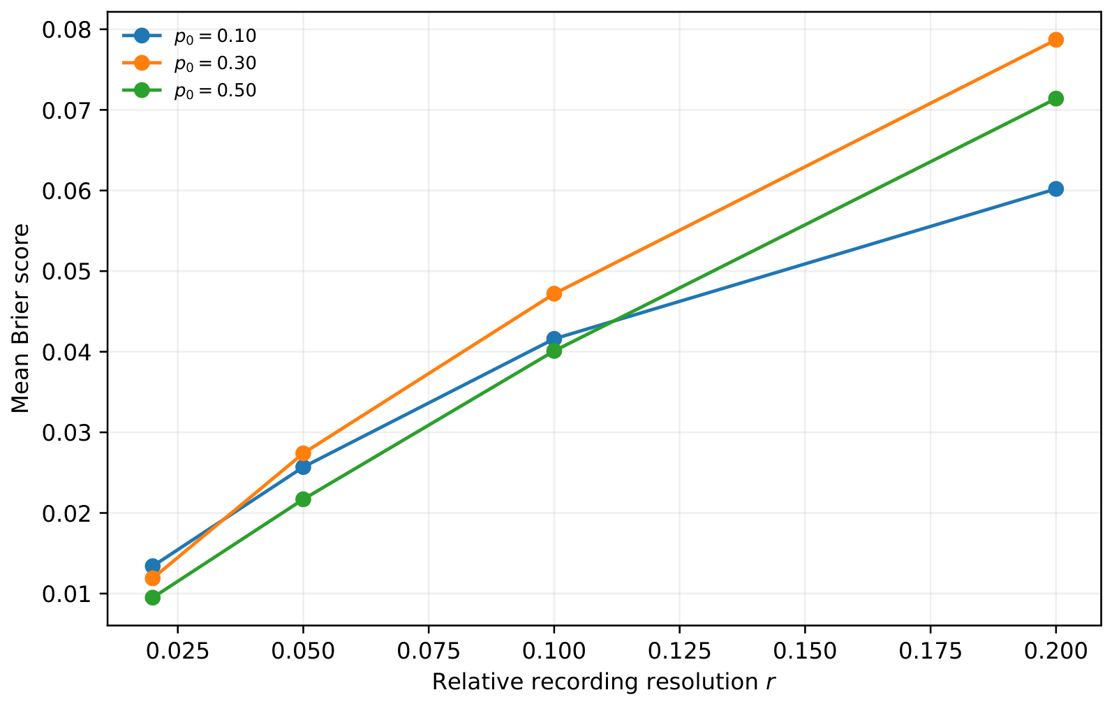
Posterior common-shock probabilities remain informative under fine recording but become less discriminating as the grid becomes coarser. At , the mean Brier score increases from 0.0119 at to 0.0787 at ; the corresponding changes are 0.0134 to 0.0602 for and 0.0095 to 0.0714 for . Figure 6 summarizes the corresponding Brier scores.
Figure 6.
Mean Brier score for posterior common-shock membership. Smaller values indicate better probabilistic classification.
3.5. Regular Parameters and Robustness to Asymmetric Idiosyncratic Shocks
The interval-aware rate and shape estimates display substantially more stable behavior than in the main rounded design. Table 4 shows conditional coverage generally near nominal across the main rounded design.
Table 4.
Performance of the interval-aware estimator for regular model parameters. Entries are RMSE (conditional 95% Wald coverage); the last column gives RMSE(). The Hessian-availability denominators are the same as those for in Table 3; these intervals use the frozen numerical-curvature rule described in Table 1.
Table 5 reports the comparison across idiosyncratic shock-rate configurations.
Table 5.
Robustness of to asymmetric idiosyncratic shock rates at . Coverage is conditional on a finite Hessian-based standard error.
At , the balanced and asymmetric shock designs yield very similar RMSE curves. At , RMSE () is 0.01188, 0.01242, and 0.01199 for , respectively, with no weak-identification events in these scenarios.
3.6. Direct Comparison for Regular Parameters
Table 6 compares regular-parameter RMSE for the two estimators.
Table 6.
Direct comparison on the same 1000 replications per scenario. Entries are RMSE (interval-aware/midpoint). Complete biases, conditional coverages and denominators appear in Supplementary Table S1.
The archived simulation objects contain both estimators on the same samples. Their first 1000 replications were checked against the retained summaries. For or , the midpoint-to-interval RMSE ratio ranges from 4.81 to 14.11 for , 1.99 to 12.95 for , and 4.00 to 9.88 for . Shape-parameter ratios are smaller (1.03–1.58). At , however, midpoint RMSE is lower for all three rates and for . At , it is also slightly lower for . There is no uniform dominance across parameters or scenarios.
For example, at , interval-aware versus midpoint bias is 0.0020 versus 0.7776 for , 0.00002 versus 0.4378 for , and 0.0008 versus for . Conditional coverage is approximately 0.950, 0.948 and 0.954 for the interval-aware rates (676 eligible replications), versus 0, 0.017 and 0 for midpoint (1000 eligible replications). These are method-specific conditional summaries, not coverages on a common selected subset; midpoint intervals are additionally conditional on the chosen pseudo-support. Point-estimate RMSE uses all 1000 replications per method.
3.7. Numerical Benchmark Results
A targeted serial benchmark used R 4.2.2 Patched under Ubuntu 24.04.3 LTS on an Intel Xeon Platinum 8573C host, seed 19102026 and base R only. For each , 20 independent samples of size 250 were generated with , and . Both rate methods used the same sample and fixed true . Direct L-BFGS-B started at rates , with log-rate bounds , maximum 1500 iterations, factr and pgtol. Profiling used the frozen root tolerance. All 60 profiling solutions were finite and all direct fits returned convergence code zero. The maximum absolute log-likelihood difference was and maximum absolute rate difference was . Median elapsed time per call was 0.700 ms for profiling and 12.800 ms for joint optimization (ten calls per sample). These timings concern fixed shape and slope, not full five-parameter estimation or universal computational superiority. Probability verification used 72 cases: three singular masses, four resolutions and six geometries (ray-crossing, above-ray, below-ray, origin, tail and a cell with side length ). The reference uses nested adaptive integrate calls on both continuous regions, split at corner/ray intersections, plus a separate numerical singular integral. Relative tolerance is , absolute tolerance and the subdivision limit 500. The singular integral is independently evaluated, not reused from the explicit formula. Maximum absolute probability discrepancy was . For the five ordinary geometries, the maximum relative discrepancy was ; tiny-cell relative discrepancy reached , although absolute error stayed below . This exposes cancellation rather than certifying relative accuracy for arbitrarily small cells. Median scalar-cell times were 0.087 ms for explicit evaluation and 1.333 ms for quadrature (1000 and three calls per case). All quadrature calls returned without errors. R overhead, host load and timer resolution affect these timings; case-level errors, timings and session information accompany this revision.
4. Exploratory Computational Illustration: Asynchronous River Responses
4.1. Temporal Estimand and Observational Definition
We considered the processed IDEAM river-level snapshot (maximum-level and instantaneous-level products, snapshot date 19 September 2026) from Montería-AUT (13067020) and Cotocá Abajo-AUT (13077060) [40,41]. The purpose was joint estimation of for temporal responses, allowing a common-shock component to generate non-simultaneous station responses. Here, X denotes the time to the first recorded attainment of an episode maximum at Cotocá and Y the corresponding time at Montería, both measured from a common operational episode origin. A singular slope fitted to level excesses would describe a magnitude ratio rather than a temporal-delay parameter; the present application therefore explicitly uses temporal responses.
Under the model’s singular component, . Thus, is a dimensionless temporal factor, and the associated signed delay is
In this orientation, denotes a later Cotocá response, whereas denotes an earlier response. The model does not impose a constant additive delay, and not every observation has to belong to the singular component.
The physical shock time was not observed. We used the beginning of the first union-exceedance day of an episode as an operational origin. An attainment occurring k calendar days later was represented by the daily cell . These are grouped operational response times, not observed exact shock-to-peak durations. The cell was retained when the response occurred on the first day; no artificial one-day shift was imposed.
4.2. Asynchronous Event Construction and Peak-Date Audit
All available station dates between 18 March 2019 and 10 September 2026 were retained for episode detection and extraction. Peaks were not required to occur on the same day, and days observed at only one station were not discarded at this stage. To preserve the original threshold calibration, marginal quantiles were estimated from the 624 dates with observations in both stations. Calibration on shared dates does not impose simultaneous response dates. A separate sensitivity analysis used all available dates for each station.
At , the thresholds were 3.26 m at Montería and 5.687 m at Cotocá. Days exceeding either threshold were grouped when separated by at most five calendar days. Episodes were retained if both station maxima exceeded their thresholds somewhere within the resulting window. This rule permits asynchronous responses but does not prove a shared physical cause or temporal independence.
Table 7 lists the two grouped temporal observations under the primary definition.
Table 7.
Primary temporal observations. X refers to Cotocá and Y to Montería. Date differences use first recorded attainment of each maximum.
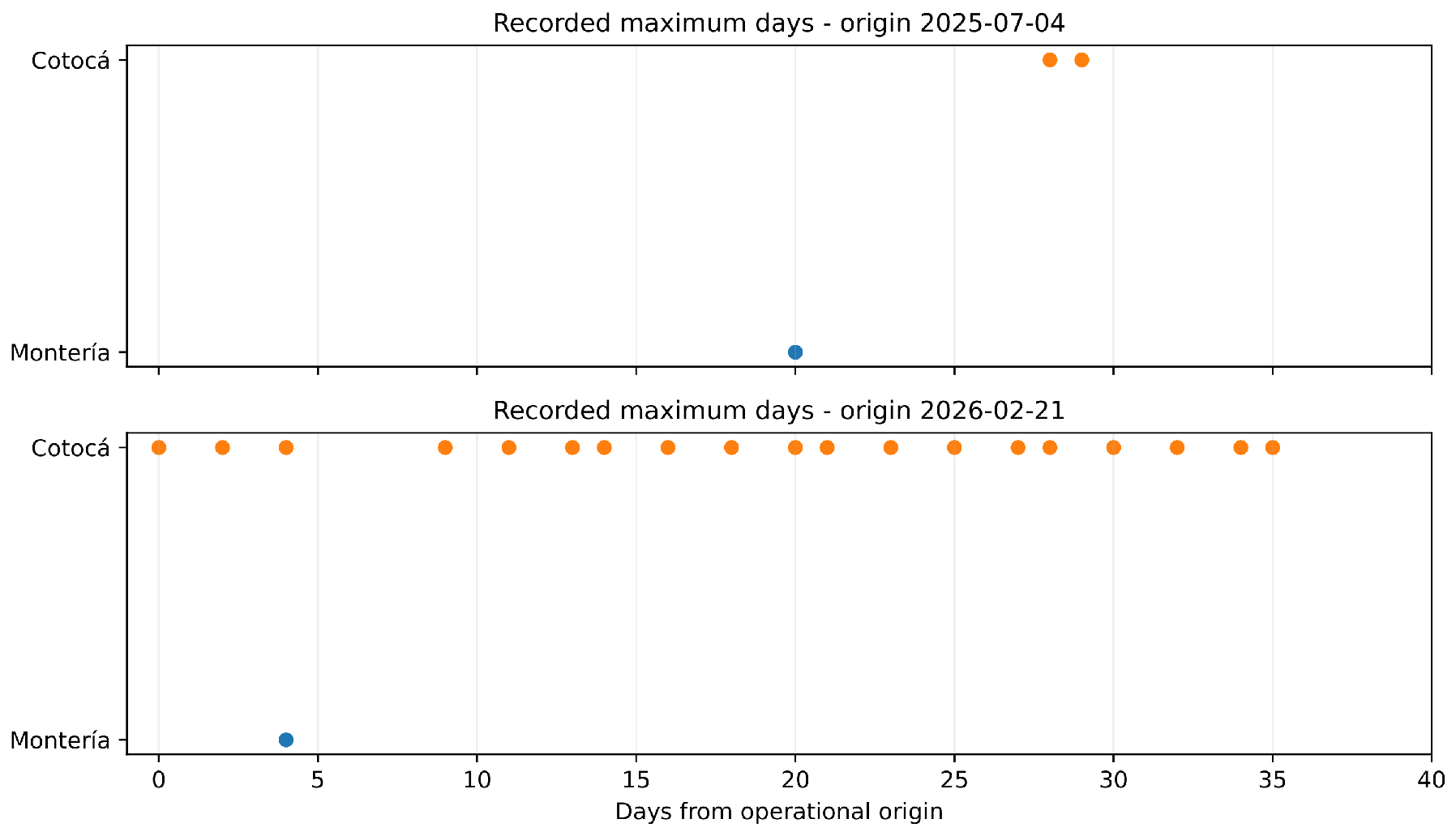
The 2026 Cotocá maximum, 7.64 m, occurred on 19 recorded days between 21 February and 28 March. Consequently, the date difference of minus four days does not identify a unique peak or a flood travel time. Using the last recorded attainment instead gives differences of 9 and 31 days for the two episodes. Such repeated recorded maxima may reflect discretization, stable levels, or instrumental issues; the supplied data do not distinguish these explanations. First and last attainment define different response variables, and this distinction was explicitly examined.
Figure 7 displays all recorded maximum-attainment days.
Figure 7.
All recorded days attaining each episode’s station maximum, measured from the operational common origin. Cotocá’s 2026 maximum is tied on 19 days; first and last attainment are therefore different temporal responses rather than alternative measurements of a unique observed peak. Orange dots represent Cotocá and blue dots represent Montería; each dot marks a recorded maximum-attainment day.
4.3. Joint Interval Likelihood and Computational Procedure
For the survival function in Equation (2), the contribution of each observed temporal rectangle is Equation (24). We optimized jointly over all five parameters; marginal fits were not performed first to obtain a subsequent ratio estimate. The rectangle likelihood includes singular-line probability and does not replace grouped times by exact midpoints.
For numerical scaling, both times were divided by ten days. Rates reported in day units were transformed back using . Corner-ratio breakpoints in defined search regions. Within each region, multiple global starts were followed by bounded local refinement. Scaled rates were bounded by and by . Results are the best numerical bounded solutions found, not certified global or interior maxima.
Table 8 reports the primary bounded joint fit.
Table 8.
Joint temporal fit under the primary operational definition. Rates are in day units, with dimension .
The scaled second rate reached its lower bound, . The small day-scale value must therefore not be interpreted as a precise estimate of a negligible mechanism. The fitted singular probabilities conditional on the two rectangles were 0.98425 and zero, respectively. These are model-internal classifications, not validated causal probabilities for physical hydrological shocks.
Conditionally on the singular component, implies a Cotocá time 40% larger than the Montería time. For days, this gives days and an eight-day difference, matching the first-attainment dates of the 2025 episode. The 2026 pair is instead attributed to the continuous component under this solution. This interpretation applies to the selected origin and response definition, not to a general fixed station-to-station travel time.
Figure 8 displays the fitted joint survival surface and its level sets, including the non-diagonal singular line. Figure 9 shows total one-day cell probabilities and fitted conditional singular-component probabilities. The displayed cell domain contains approximately 0.849 of the model probability and is not renormalized. Figure 10 compares fitted marginal CDFs with empirical bounds induced by daily grouping. With two responses per margin, these are descriptive diagnostics rather than goodness-of-fit evidence.
4.4. Profile Likelihood and Sensitivity to Observational Definition
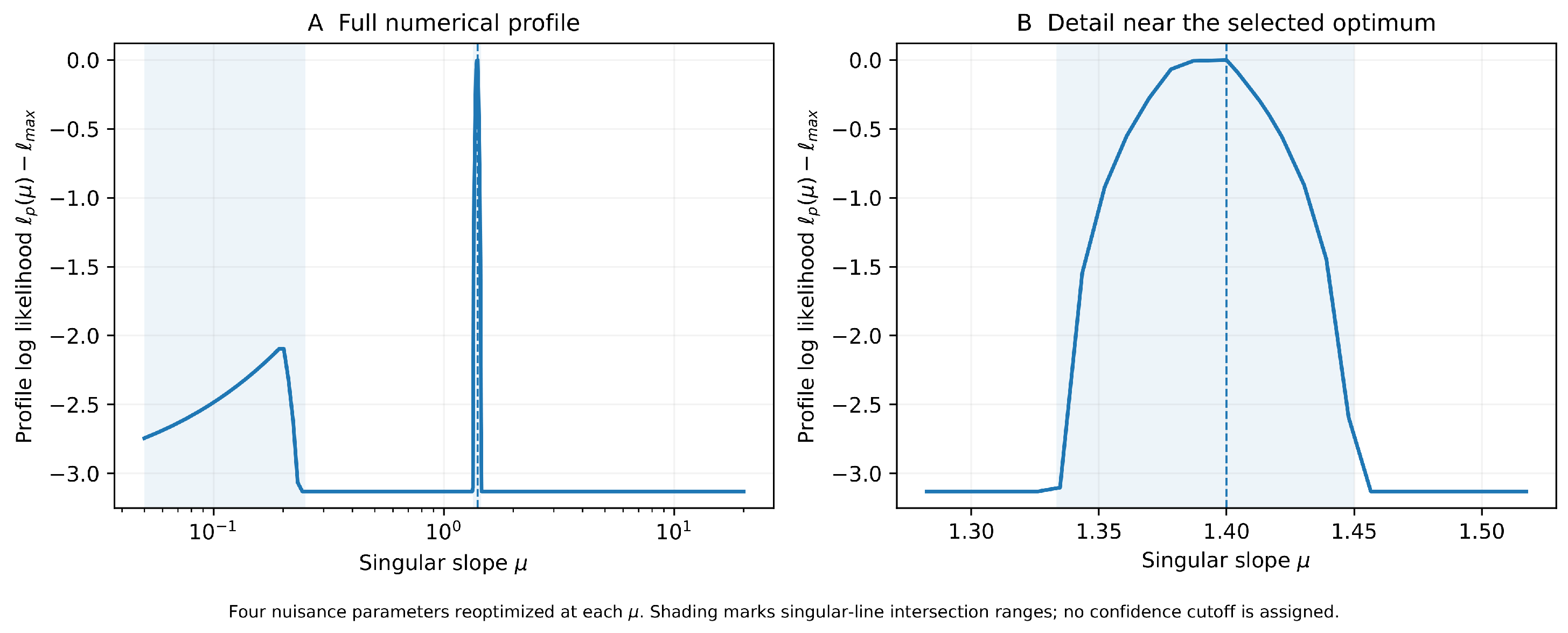
We recomputed a nuisance-profiled likelihood at 180 values of over the search range, using multiple starts for the four remaining parameters at each point. The maximum remains near 1.40; the four nuisance parameters are reoptimized along the curve rather than held fixed. The shaded geometric ranges are not confidence intervals, and no uncalibrated likelihood-ratio cutoff is imposed.
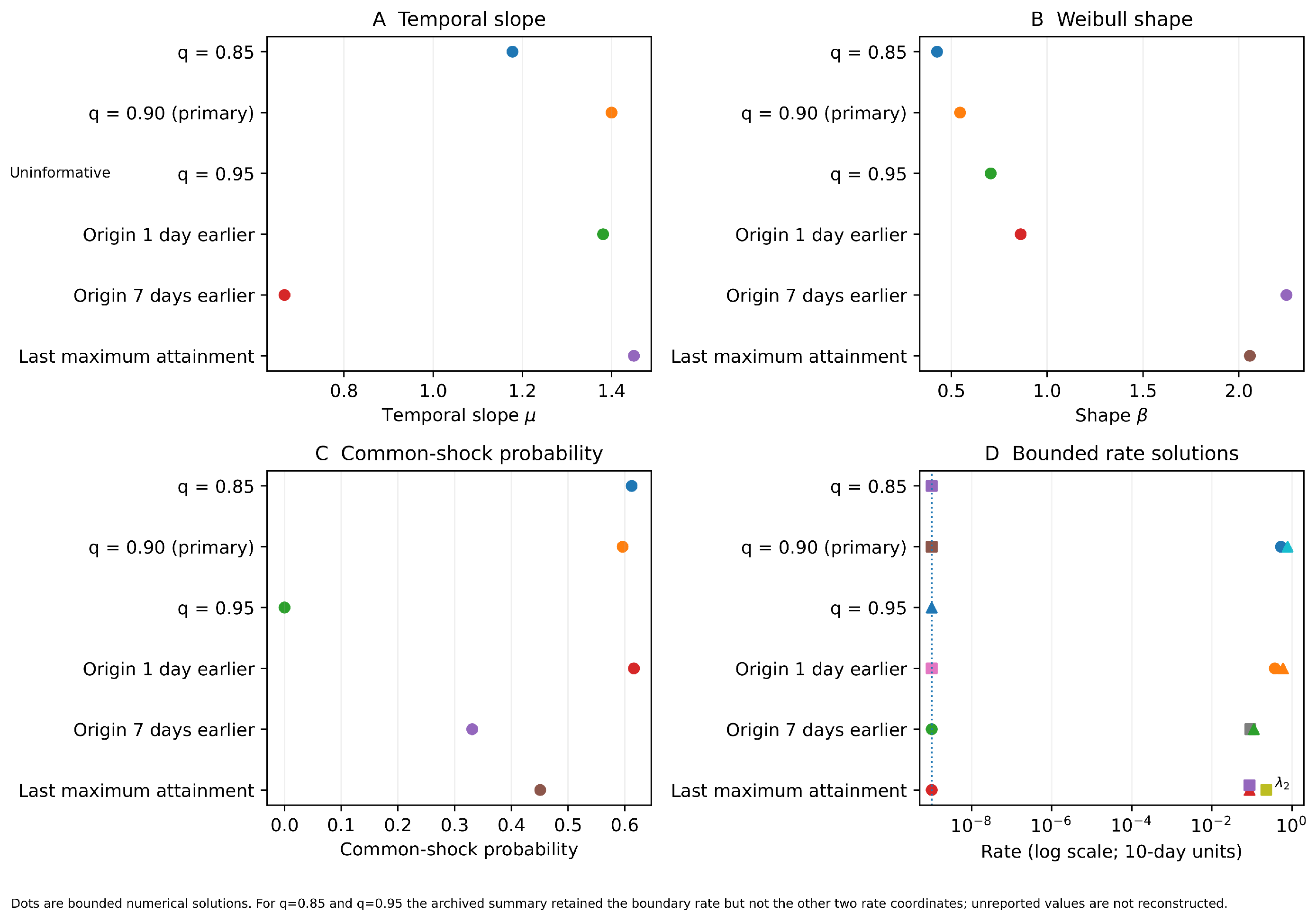
At , the optimizer returned a slope near its lower bound, but and the common-shock rate approached zero. In this near-independence configuration, the slope is practically uninformative, so its numerical value is not reported as a meaningful delay factor. Calibrating thresholds from all available dates per station left only one joint episode at and ; these samples were documented but not used to claim five-parameter inference.
Figure 8.
Joint survival surface and contours for the primary temporal MOBW- fit. The marked line is ; rectangles identify the two grouped observations. The survival law incorporates both continuous and singular probability.
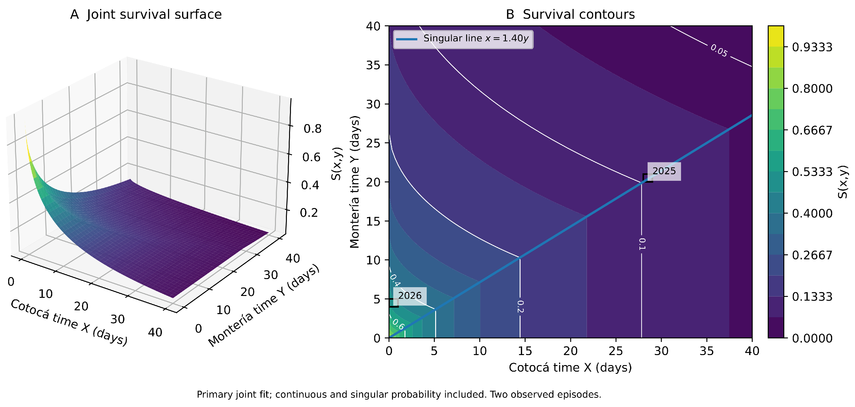
Figure 9.
Total probabilities of one-day response cells (left, logarithmic scale) and fitted conditional singular-component probabilities (right). The displayed domain contains approximately 0.849 of model probability, without renormalization. Conditional singular probabilities are internal model classifications.
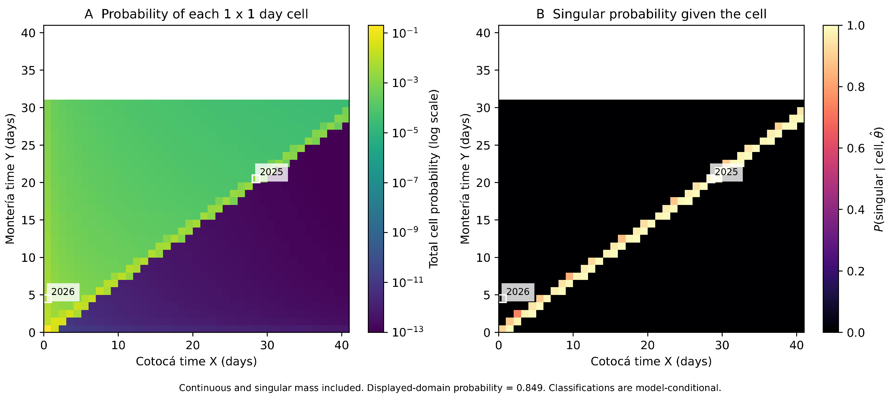
Figure 10.
Fitted marginal cumulative distributions and empirical CDF bounds induced by daily grouping. Shading represents grouping uncertainty, not sampling confidence bands. With two observations per margin, the comparison is descriptive. The blue curve is the fitted marginal CDF. The orange and green step curves delimit the empirical CDF bounds induced by the daily observation cells.
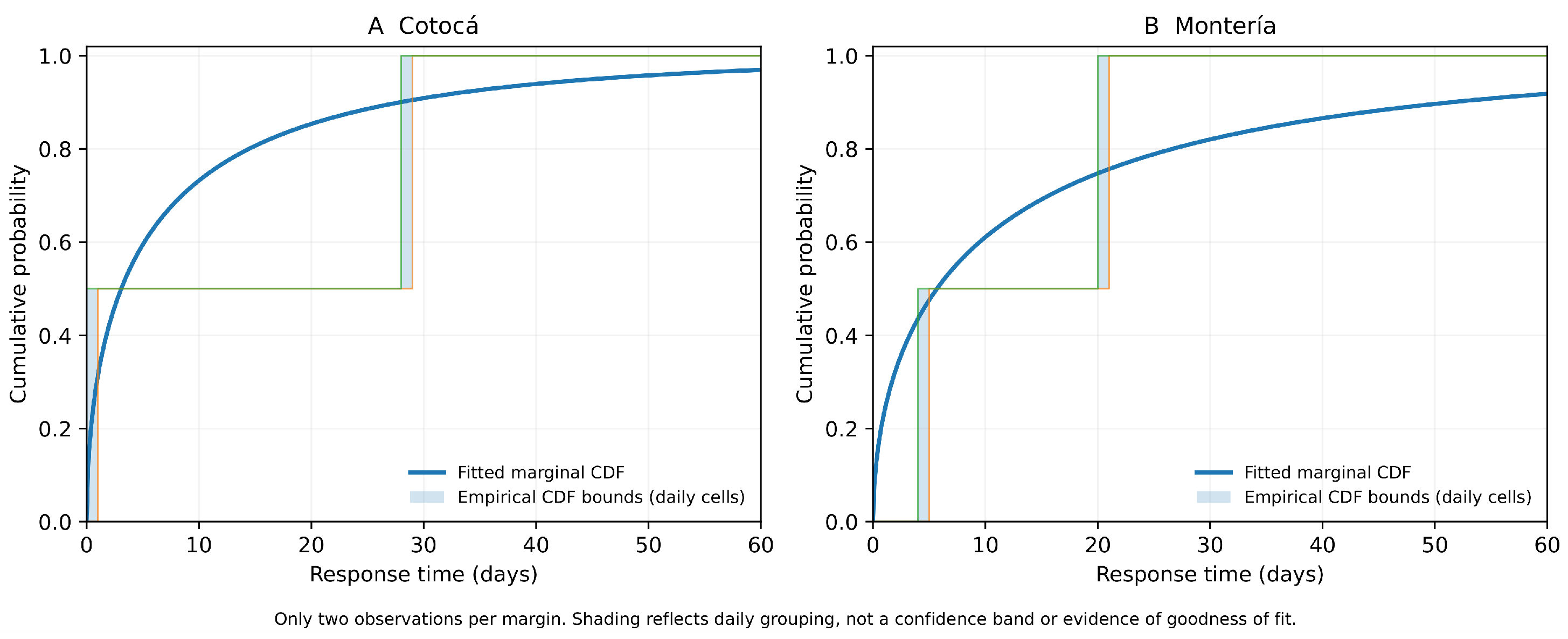
Figure 11 displays the resulting profile and a detail near the selected optimum.
Figure 11.
Bounded numerical profile likelihood for over the full search range and near the selected optimum. Four nuisance parameters were reoptimized at each of 180 slope values. No conventional likelihood-ratio confidence cutoff is assigned. The vertical dashed line marks the selected slope .
Moving an origin c days earlier gives and . A singular relation transforms as
Except when , the translated singular line does not pass through the new origin. MOBW- is therefore not invariant to arbitrary origin changes. In the present sample, a seven-day shift changed the preferred singular assignment from the 2025 episode to the 2026 episode despite leaving station-date differences unchanged. Origin selection is therefore part of the scientific model definition.
4.5. Scientific Interpretation and Scope
This temporal application establishes that the proposed likelihood can be used for joint numerical estimation with non-simultaneous operational responses. It also illustrates the distinction between a multiplicative temporal factor and an additive delay. However, the available sample consists of only two episodes, the best solutions reach rate boundaries, and the inferred singular geometry depends strongly on operational origin and response definition. Standard Wald intervals, Hessian errors, conventional likelihood-ratio calibration, and confirmatory model rankings are consequently not reported.
The physical shock origin was not observed, and the responses were selected retrospectively from threshold-defined episodes. Hence, the working likelihood does not establish that the derived times follow the generative shock mechanism. The supplied cleaning rules, unit conversions, and repeated maximum values also require station-level validation. No imputation or new historical download was performed. The application should be described as exploratory rather than as a robust estimate of a systematic hydrological delay or a principal empirical validation of MOBW-.
With two episodes, this illustration does not validate a five-parameter hydrological model. It demonstrates likelihood evaluation, bounded fitting and sensitivity diagnostics. Model-based membership probabilities are not independently validated physical shock labels; a larger collection of independently validated events is needed for substantive hydrological inference.
5. Discussion
This study addresses a specific inferential gap left by the original development of the MOBW- distribution [23]. In the exact model, the displaced singularity can be statistically advantageous because repeated support ratios identify almost surely once at least two common shocks are observed. That behavior differs fundamentally from ordinary smooth-parameter estimation. The same feature, however, makes the model sensitive to finite recording resolution: once an observation is represented by a rectangle rather than an exact point, the singular line is no longer directly observed.
The Monte Carlo results show that midpoint substitution is not a harmless approximation in this setting. For moderate and large singular masses, the interval-aware likelihood produces substantially smaller RMSE for and substantially reduces the positive bias induced by midpoint substitution. This occurs because the rectangle likelihood in Equation (24) respects the probability mass contributed by the singular component wherever the line intersects with the observed cell. More generally, the result reinforces earlier warnings that rounded or coarse observations should be analyzed through their observation sets rather than be automatically treated as exact measurements [32,36,37].
The low-singular-mass regime provides an equally important result. When , the method does not simply fail numerically. Instead, some samples develop broad or competing profile-likelihood modes for . The operational weak-identification diagnostic separates these samples from the remainder, and in the difficult setting, the RMSE difference between weak and non-weak samples is substantial. This distinction is consistent with the broader literature, showing that weak information can invalidate local quadratic approximations even when an optimizer returns a nominally successful estimate [26,27,39]. It also explains why Hessian-based standard errors for are not available in every replication and why the reported Wald coverage is conditional on the finite curvature.
The temporal application clarifies a separate issue that does not arise when simulation origins are fixed by design. A common-shock relation permits asynchronous responses, but it defines a proportional temporal factor rather than a constant additive lag. Translating an operational origin adds an intercept to the singular line unless . The origin sensitivity in Table 9 and Figure 12 consequently reflects a change in observational definition and model geometry, not merely numerical instability. The fitted slope of 1.40 must not be read as a robust 40% hydrological delay from these two episodes. The likelihood profile is useful precisely because it makes the conditional geometry visible without resolving these design limitations.
Table 9.
Sensitivity of the joint numerical fit. Every row reaches a rate boundary.
The direct regular-parameter comparison supports lower rate-parameter RMSE for interval-aware estimation at moderate and large singular masses, but not uniform improvement in shape estimation. The regular parameters behave more conventionally. Exact-data coverage is near nominal across the 17 benchmark scenarios, and under rounding, the interval-aware estimator maintains acceptable RMSE and coverage for , , , and . The robustness analysis further shows that asymmetry in the two idiosyncratic shock rates has relatively little effect on the estimation of when singular mass is moderate. These findings complement earlier work on likelihood, EM, Bayesian, censoring, and reliability inference for Marshall–Olkin Weibull models [12,13,14,17,18,19,22].
Several limitations define useful directions for extension. First, the current simulations use a common Weibull shape parameter and a common recording width on both margins; unequal grid widths and more general marginal structures deserve separate study. Second, the paper focuses on estimation and profile diagnostics rather than a fully calibrated likelihood-ratio testing theory for . Third, censoring, truncation, and stochastic coarsening mechanisms are outside the current design, although the rectangle-likelihood formulation provides a natural starting point. Finally, the Sinú application is an exploratory observational illustration rather than a principal empirical validation. It uses only two threshold-defined episodes, an operational rather than observed physical shock origin, and response dates affected by tied recorded maxima. Its boundary solutions and sensitivity results limit substantive hydrological interpretation. More informative event collections, validated station records, and scientifically defensible origins are required before estimating a systematic physical delay.
Figure 12.
Sensitivity of the bounded solutions to threshold, operational origin, and first-versus-last maximum attainment. Panels show the singular slope, Weibull shape, common-shock probability and rate-boundary behavior. Points are fitted solutions, not uncertainty intervals. At , negligible common-shock mass leaves the slope practically uninformative. Colors identify the six specifications listed on the vertical axes: blue, ; orange, the primary fit; green, ; red, an origin one day earlier; purple, an origin seven days earlier; and brown, last maximum attainment. In panel D, circles, squares and triangles denote , and , respectively; the vertical dashed line marks the lower bound for the scaled rates. Only archived rate coordinates are displayed.
From an inferential perspective, the simulations also clarify why the model should not be treated as an ordinary five-parameter smooth family. Under exact observation, can be identified geometrically through repeated support ratios, a mechanism qualitatively different from Fisher-information accumulation for regular rate and shape parameters. Under rounding, that exact mechanism disappears and information about becomes continuous but potentially weak. The resulting profile can be sharply peaked when is moderate or large and broad or multimodal when is small. This transition is consistent with the general likelihood view that weak identification is fundamentally a lack of curvature/information rather than a synonym for numerical nonconvergence [26,27].
The coarse-data perspective is equally important. Rounding is not modeled as additive noise; it changes the observed sigma-field by replacing a latent point with a known rectangle. Under fixed grids this is a grouped-data likelihood problem, so Equation (24) is the direct likelihood contribution of the observed event [32,36]. Midpoint substitution can therefore be severely biased even when the grid appears visually fine because it changes whether an observation is treated as lying on, above, or below a parameter-dependent singular support. The effect is geometric as well as numerical.
6. Conclusions
Likelihood inference for the MOBW- model requires explicit attention to the singular support. Under exact observation, repeated common-shock ratios can recover exactly with a simple finite-sample probability determined by n and . Under finite recording resolution, the correct likelihood contribution is the probability of an observed rectangle, not the density evaluated at an arbitrary representative point.
The simulation study demonstrates three main conclusions. First, the exact benchmark is numerically stable and yields near-nominal frequentist coverage. Second, for moderate and large singular masses, the interval-aware estimator provides substantially lower bias and RMSE for than the specified midpoint comparator, and lower rate-parameter RMSE at moderate and large singular masses; shape accuracy is similar and not uniformly improved. Third, when singular mass is small and recording is coarse, inference for can become weakly identified; profile-likelihood diagnostics reveal this limitation even when numerical optimization succeeds. These results provide a practical inference framework for a singular bivariate lifetime model and clarify the boundary between numerical estimation error and genuine lack of information about the modified singularity.
The river-response illustration extends the computational framework to asynchronous grouped times while emphasizing its observational requirements. Joint optimization alone does not establish empirical identification: the selected rate boundary, repeated recorded maxima, and origin dependence preclude a robust hydrological-delay conclusion. Clear response definitions and validated observation mechanisms are therefore as important as preserving singular mass in the likelihood.
Supplementary Materials
The following supporting information can be downloaded at: https://www.mdpi.com/article/10.3390/math14213999/s1. The revision supplement additionally contains the R numerical-verification script, case-level benchmark results, the complete regular-parameter comparison and the audited numerical settings. These new files are supplied with this revision and are not asserted to be part of the original Zenodo v1.0.0 release. The original supporting information comprises: Supplementary File S1, MOBWReproducibilitySupplement.zip, containing the R code for likelihood evaluation and estimation of the MOBW- model, the complete Monte Carlo simulation workflow, simulation summaries, the processed data used in the Sinú River application, profile-likelihood analyses, and the scripts required to reproduce the tables and figures reported in the manuscript. For long-term preservation and reproducibility, the complete package is also permanently archived in Zenodo as MOBW-mu Likelihood Inference Reproducibility Materials, Version 1.0.0 [42], available at https://doi.org/10.5281/zenodo.22864671, 20 October 2026. Table S1: Bias, root mean squared error (RMSE), and conditional coverage of nominal 95% Wald intervals for the rate and shape parameters.
Author Contributions
Conceptualization, H.B.; methodology, H.B.; software, H.B.; validation, H.B. and J.R.-M.; formal analysis, H.B.; investigation, H.B.; data curation, H.B.; writing—original draft preparation, H.B. and J.R.-M.; writing—review and editing, H.B. and J.R.-M.; visualization, H.B. and J.R.-M.; project administration, H.B. and J.R.-M. All authors have read and agreed to the published version of the manuscript.
Funding
This research was funded by Vice-rectorate for Research of the Universidad de Córdoba, Colombia, project grant FCB-02-24: “Modelos estadísticos aplicados a eventos dependientes” (J.R.-M.).
Institutional Review Board Statement
Not applicable. This methodological study uses Monte Carlo simulation and processed environmental river-level observations and does not involve human participants or animal experiments.
Informed Consent Statement
Not applicable.
Data Availability Statement
The processed data used in the application, the R source code for likelihood evaluation and parameter estimation, the Monte Carlo simulation code and summaries, the profile-likelihood analyses, and the scripts for the original tables and figures are openly available in Zenodo in the repository MOBW-mu Likelihood Inference Reproducibility Materials, Version 1.0.0 [42], available at https://doi.org/10.5281/zenodo.22864671, 20 October 2026. The original hydrological observations used to construct the Sinú River application were obtained from the Colombian Institute of Hydrology, Meteorology and Environmental Studies (IDEAM). The Zenodo repository contains the processed dataset used in the statistical analyses reported in this article.
Acknowledgments
The authors gratefully acknowledge the Universidad de Córdoba, Colombia, for financial support and Universidad de Sucre. During the preparation of this manuscript, the authors used ChatGPT (OpenAI, GPT-6.1 Sol) for language editing and organizational support. The authors reviewed and edited the output and take full responsibility for the content of this publication.
Conflicts of Interest
The authors declare no conflicts of interest.
Abbreviations
The following abbreviations are used in this manuscript:
| CDF | Cumulative distribution function |
| EM | Expectation–maximization |
| IDEAM | Instituto de Hidrología, Meteorología y Estudios Ambientales |
| MOBW | Marshall–Olkin bivariate Weibull |
| MOBW- | Marshall–Olkin bivariate Weibull model with modified singularity |
| RMSE | Root mean squared error |
| SE | Standard error |
References
- Marshall, A.W.; Olkin, I. A Multivariate Exponential Distribution. J. Am. Stat. Assoc. 1967, 62, 30–44. [Google Scholar] [CrossRef]
- Marshall, A.W.; Olkin, I. A Generalized Bivariate Exponential Distribution. J. Appl. Probab. 1967, 4, 291–302. [Google Scholar] [CrossRef] [Scilit]
- Barlow, R.E.; Proschan, F. Statistical Theory of Reliability and Life Testing: Probability Models; To Begin With: Silver Spring, MD, USA, 1982. [Google Scholar]
- Singpurwalla, N.D. Reliability and Risk: A Bayesian Perspective; Wiley: Hoboken, NJ, USA, 2006. [Google Scholar]
- Basu, A.P. Bivariate Failure Rate. J. Am. Stat. Assoc. 1971, 66, 103–104. [Google Scholar] [CrossRef]
- Johnson, N.L.; Kotz, S. A Vector-Valued Multivariate Hazard Rate. J. Multivar. Anal. 1975, 5, 53–66. [Google Scholar] [CrossRef] [Scilit]
- Marshall, A.W. Some Comments on Hazard Gradient. Stoch. Process. Appl. 1975, 3, 293–300. [Google Scholar] [CrossRef] [Scilit]
- McNeil, A.J.; Frey, R.; Embrechts, P. Quantitative Risk Management: Concepts, Techniques and Tools, Revised ed.; Princeton University Press: Princeton, NJ, USA, 2015. [Google Scholar]
- Bayramoglu, I.; Ozkut, M. Recent Developments about Marshall–Olkin Bivariate Distribution. J. Stat. Theory Pract. 2022, 16, 58. [Google Scholar] [CrossRef] [Scilit]
- Bemis, B.M.; Bain, L.J.; Higgins, J.J. Estimation and Hypothesis Testing for the Parameters of a Bivariate Exponential Distribution. J. Am. Stat. Assoc. 1972, 67, 927–929. [Google Scholar] [CrossRef]
- Karlis, D. ML Estimation for Multivariate Shock Models via an EM Algorithm. Ann. Inst. Stat. Math. 2003, 55, 817–830. [Google Scholar] [CrossRef] [Scilit]
- Kundu, D.; Dey, A.K. Estimating the Parameters of the Marshall–Olkin Bivariate Weibull Distribution by EM Algorithm. Comput. Stat. Data Anal. 2009, 53, 956–965. [Google Scholar] [CrossRef] [Scilit]
- Kundu, D.; Gupta, A.K. Bayes Estimation for the Marshall–Olkin Bivariate Weibull Distribution. Comput. Stat. Data Anal. 2013, 57, 271–281. [Google Scholar] [CrossRef] [Scilit]
- Shen, Y.; Xu, A. On the Dependent Competing Risks Using the Marshall–Olkin Bivariate Weibull Model: Parameter Estimation with Different Methods. Commun. Stat. Theory Methods 2018, 47, 5558–5572. [Google Scholar] [CrossRef] [Scilit]
- Feizjavadian, S.H.; Hashemi, R. Analysis of Dependent Competing Risks in the Presence of Progressive Hybrid Censoring Using the Marshall–Olkin Bivariate Weibull Distribution. Comput. Stat. Data Anal. 2015, 82, 19–34. [Google Scholar] [CrossRef] [Scilit]
- Cai, J.; Shi, Y.; Liu, B. Analysis of Incomplete Data in the Presence of Dependent Competing Risks from the Marshall–Olkin Bivariate Weibull Distribution under Progressive Hybrid Censoring. Commun. Stat. Theory Methods 2017, 46, 6497–6511. [Google Scholar] [CrossRef] [Scilit]
- Bai, X.; Shi, Y.; Liu, B.; Fu, Q. Statistical Inference of the Marshall–Olkin Bivariate Weibull Distribution with Three Shocks Based on Progressive Interval-Censored Data. Commun. Stat. Simul. Comput. 2019, 48, 637–654. [Google Scholar] [CrossRef] [Scilit]
- Bai, X.; Shi, Y.; Ng, H.K.T.; Liu, Y. Inference of an Accelerated Dependent Competing Risks Model for the Marshall–Olkin Bivariate Weibull Distribution with Nonconstant Parameters. J. Comput. Appl. Math. 2020, 366, 112398. [Google Scholar] [CrossRef] [Scilit]
- Zhang, L.; Xu, A.; An, L.; Li, M. Bayesian Inference of System Reliability for a Multicomponent Stress–Strength Model under the Marshall–Olkin Weibull Distribution. Systems 2022, 10, 196. [Google Scholar] [CrossRef] [Scilit]
- Dutta, S.; Kayal, S. Statistical Inference for Dependent Competing Risks Data under Adaptive Type-II Progressive Hybrid Censoring. J. Appl. Stat. 2025, 52, 1871–1903. [Google Scholar] [CrossRef] [Scilit] [PubMed]
- Hanagal, D.D. A Bivariate Weibull Regression Model. Stoch. Qual. Control 2005, 20, 143–150. [Google Scholar] [CrossRef] [Scilit]
- Kumar, S.; Kundu, D.; Mitra, S. Estimation of Five-Parameter Bivariate Modified Weibull Singular Distribution. Commun. Stat. Simul. Comput. 2026, 55, 1267–1290. [Google Scholar] [CrossRef] [Scilit]
- Brango, H.; Guerrero, A.; Llinás, H. Marshall–Olkin Bivariate Weibull Model with Modified Singularity (MOBW-μ): A Study of Its Properties and Correlation Structure. Mathematics 2024, 12, 2183. [Google Scholar] [CrossRef] [Scilit]
- Smith, R.L. Maximum Likelihood Estimation in a Class of Nonregular Cases. Biometrika 1985, 72, 67–90. [Google Scholar] [CrossRef]
- Self, S.G.; Liang, K.-Y. Asymptotic Properties of Maximum Likelihood Estimators and Likelihood Ratio Tests under Nonstandard Conditions. J. Am. Stat. Assoc. 1987, 82, 605–610. [Google Scholar] [CrossRef]
- Andrews, D.W.K.; Cheng, X. Estimation and Inference with Weak, Semi-Strong, and Strong Identification. Econometrica 2012, 80, 2153–2211. [Google Scholar] [CrossRef] [Scilit]
- Andrews, I.; Mikusheva, A. Weak Identification in Maximum Likelihood: A Question of Information. Am. Econ. Rev. 2014, 104, 195–199. [Google Scholar] [CrossRef] [Scilit]
- Venzon, D.J.; Moolgavkar, S.H. A Method for Computing Profile-Likelihood-Based Confidence Intervals. J. R. Stat. Soc. C 1988, 37, 87–94. [Google Scholar] [CrossRef] [Scilit]
- Zhang, Z. Profile Likelihood and Incomplete Data. Int. Stat. Rev. 2010, 78, 102–116. [Google Scholar] [CrossRef] [Scilit] [PubMed]
- Raue, A.; Kreutz, C.; Maiwald, T.; Bachmann, J.; Schilling, M.; Klingmüller, U.; Timmer, J. Structural and Practical Identifiability Analysis of Partially Observed Dynamical Models by Exploiting the Profile Likelihood. Bioinformatics 2009, 25, 1923–1929. [Google Scholar] [CrossRef] [Scilit] [PubMed]
- Fischer, S.M.; Lewis, M.A. A Robust and Efficient Algorithm to Find Profile Likelihood Confidence Intervals. Stat. Comput. 2021, 31, 38. [Google Scholar] [CrossRef] [Scilit]
- Heitjan, D.F.; Rubin, D.B. Ignorability and Coarse Data. Ann. Stat. 1991, 19, 2244–2253. [Google Scholar] [CrossRef] [Scilit]
- Heitjan, D.F.; Rubin, D.B. Inference from Coarse Data via Multiple Imputation with Application to Age Heaping. J. Am. Stat. Assoc. 1990, 85, 304–314. [Google Scholar] [CrossRef]
- Heitjan, D.F. Ignorability and Coarse Data: Some Biomedical Examples. Biometrics 1993, 49, 1099–1109. [Google Scholar] [CrossRef] [Scilit]
- Lindley, D.V. Grouping Corrections and Maximum Likelihood Equations. Proc. Camb. Philos. Soc. 1950, 46, 106–110. [Google Scholar] [CrossRef] [Scilit]
- Bai, Z.; Zheng, S.; Zhang, B.; Hu, G. Statistical Analysis for Rounded Data. J. Stat. Plan. Inference 2009, 139, 2526–2542. [Google Scholar] [CrossRef] [Scilit]
- Kim, J.K. Imputation for Statistical Inference with Coarse Data. Can. J. Stat. 2012, 40, 604–618. [Google Scholar] [CrossRef] [Scilit]
- Li, Y.; Sun, J.; Song, S. Statistical analysis of bivariate failure time data with Marshall–Olkin Weibull models. Comput. Stat. Data Anal. 2012, 56, 2041–2050. [Google Scholar] [CrossRef] [Scilit] [PubMed]
- Andrews, I.; Mikusheva, A. Maximum Likelihood Inference in Weakly Identified Dynamic Stochastic General Equilibrium Models. Quant. Econ. 2015, 6, 123–152. [Google Scholar] [CrossRef] [Scilit]
- Instituto de Hidrología, Meteorología y Estudios Ambientales (IDEAM). Nivel Máximo del Río. Available online: https://www.datos.gov.co/resource/vfth-yucv (accessed on 19 September 2026).
- Instituto de Hidrología, Meteorología y Estudios Ambientales (IDEAM). Nivel Instantáneo del Río. Available online: https://www.datos.gov.co/resource/bdmn-sqnh (accessed on 19 September 2026).
- Brango, H. MOBW-mu Likelihood Inference Reproducibility Materials; Version 1.0.0; Zenodo: Geneva, Switzerland, 2026. [Google Scholar] [CrossRef]

Disclaimer/Publisher’s Note: The statements, opinions and data contained in all publications are solely those of the individual author(s) and contributor(s) and not of MDPI and/or the editor(s). MDPI and/or the editor(s) disclaim responsibility for any injury to people or property resulting from any ideas, methods, instructions or products referred to in the content. |
© 2026 by the authors. Licensee MDPI, Basel, Switzerland. This article is an open access article distributed under the terms and conditions of the Creative Commons Attribution (CC BY) license.