


Abstract
Extreme learning machines (ELMs) solve output weights in closed form, so an optimized population of ELMs leaves open which members should form the ensemble. We report a controlled comparison of five rules for this selection step inLEA-EELM, where a Lotus Effect Algorithm (LEA) variant generates fuzzy-activation ELM candidates and members are chosen from a shared top- validation shortlist. Two rules are derived from the Fisher information of a candidate’s linear-Gaussian output stage. Because is only positive semidefinite and candidates have different hidden layers, F-complementary compares candidates by the Kullback–Leibler divergence between their predictive distributions, not by a Fisher–Rao distance. For F-norm, we prove that, with least-squares output weights, , so the rule selects the worst training fits; it is significantly worse than -norm on three of four regression benchmarks. F-complementary performs like greedy validation selection and is never significantly better. The information-geometric rules therefore add no measured benefit; the gains come from validation-guided greedy selection, which lowers test RMSE on three of four regression datasets and raises accuracy only on Satellite and Letter, but not on Letter after duplicate rows are removed. All findings are conditional on the candidate pool of a non-canonical (subtractive-sign) LEA variant.
Keywords:
extreme learning machine; information geometry; Fisher information; Kullback–Leibler divergence; selective ensemble; validation-guided selection; metaheuristic optimization; fuzzy activation function MSC:
68T07; 62B11; 62B10
1. Introduction
Extreme Learning Machines (ELMs) [1] are single-hidden-layer feedforward networks in which hidden-layer weights and biases are assigned randomly, and only the output weights are solved analytically, via a Moore–Penrose pseudoinverse. The resulting training speed is a genuine advantage over gradient-trained networks, but it comes with a well-known cost: two independently drawn hidden layers on the same data can generalize very differently. A single, fixed activation applied uniformly across the input space adds a second source of mismatch whenever local noise or class overlap would favor a different response.
Metaheuristic search can replace the random draw with an optimized population of hidden-layer encodings. That step improves candidate quality, yet it does not by itself produce a reliable ensemble. Directed optimization tends to concentrate the population around similar high-fitness solutions, so member errors become correlated. Candidate quality alone is therefore insufficient: an ensemble also needs complementary errors and a selection rule that can identify them without looking at the test set.
Much of the ELM ensemble literature emphasizes how candidates are generated—independent random draws, genetic search, or other population-based updates—and treats the final subset as a secondary detail, often a simple ranking by fitness or output-weight norm. Less attention has been given to constructing a compact ensemble from an already optimized pool under a strict validation-only protocol.
The Lotus Effect Algorithm (LEA), previously introduced by members of the present research team [2], is a nature-inspired population-based optimizer designed to balance global exploration and local exploitation. Building on that optimizer, LEA-EELM applies LEA to optimize the hidden-layer weights and biases of a population of fuzzy ELM candidates. The present contribution lies in integrating this previously introduced LEA with adaptive fuzzy activation, analytical output-weight estimation, and validation-guided construction of a compact ensemble. The fuzzy adaptive activation function (FAF) of our earlier FAF-ELM study [3] modulates steepness from a Gaussian-membership estimate of each pre-activation; output weights are fitted analytically on the training split; and a selective ensemble of members is taken from the fittest candidates in the LEA-optimized candidate population. Three selection rules are compared on that same pool, followed by two rules derived from the Fisher information of the output stage (Section 3.6). The default LEA-EELM configuration selects members with the smallest output-weight norms from the 20 candidates with the lowest validation RMSE. The greedy-validation configuration sequentially selects the candidate that maximizes partial-ensemble validation performance. The greedy-complementary configuration sequentially selects candidates using a specified combination of validation performance and error complementarity. Aggregation is the member-output mean (regression) or majority vote (classification). Test inputs enter only at prediction.
The paper asks four questions, none of which requires LEA-EELM to be best overall:
- Does a moderate ensemble of optimized ELM candidates improve held-out performance relative to a single optimized candidate?
- Does validation-guided or diversity-aware selection improve on the default -norm configuration when both are applied to the same LEA-optimized candidate population, and do rules derived from the Fisher information of the output stage change that comparison?
- Does ridge regularization of the output weights help the tested pipeline?
- How does FAF compare with a conventional Gaussian activation on the same backbone, and how does the full pipeline compare with task-specific external baselines?
LEA-EELM is a framework for generating and selectively combining optimized ELM candidates. None of its components is new on its own: LEA, fuzzy activation, analytical output weights, and greedy ensemble selection [4] are all established. The contribution is a controlled study of the ensemble-construction stage on one shared candidate pool, including two selection rules derived from the Fisher information of the output stage, an exact explanation of why one of them fails, and an honest account of what does and does not help. The contributions are:
- An integrated learning framework that employs the previously introduced LEA to optimize fuzzy ELM candidates and subsequently constructs a compact ensemble through validation-guided member selection.
- A controlled comparison of output-weight-norm selection, established greedy ensemble selection [4], and its complementarity-weighted variant over the same LEA-optimized candidate population.
- Evidence that moderate ensembling improves over a single optimized candidate on the evaluated M-sweep datasets.
- Evidence that, relative to the default -norm configuration, validation-guided selection improves regression test RMSE on three of four regression datasets (Boston Housing is not significant after Holm adjustment), and classification accuracy on Satellite, the dataset with the largest duplicate-free validation split. The two greedy variants perform similarly.
- An information-geometric analysis of the selection step: the Fisher quadratic form of the output stage is defined only for a shared hidden layer and is a semimetric; candidates with distinct hidden layers are compared by a predictive Kullback–Leibler divergence (F-complementary), and an output-space norm rule (F-norm) is proved to select the worst training fits in the shortlist (Proposition 1). Empirically, neither rule improves on established greedy selection.
- A reproducible evaluation that identifies the useful operating conditions—regression ensemble construction—and the remaining classification challenge of selecting from small validation sets.
Against complete external baseline families (five regression baselines; seven classification baselines), LEA-EELM does not uniformly outperform every comparator. That external outcome is reported in full; it is not the claim this paper is written to establish. Section 2 situates the design; Section 3 specifies the method; Section 4 records the evaluation protocol; Section 5 reports results in the order of the questions above; and Section 6 interprets them.
2. Related Work
The ELM framework [1] trains a single-hidden-layer network by drawing input weights and biases at random and solving for output weights in closed form. That random assignment is the source of ELM’s training speed, but it also makes two independently initialized models on the same data generalize differently. Hidden-layer sensitivity is therefore a structural property of the standard ELM, not an incidental implementation detail.
Replacing the random draw with a metaheuristic search is now a standard response to that sensitivity. Genetic-ensemble ELM (GE-ELM) [5] searches hidden-layer parameters with a genetic algorithm and assembles an ensemble from the resulting population. Recent siblings use particle-swarm or related search for application-specific ELMs [6,7,8,9]. Eshtay et al. review the broader family of metaheuristic ELM design formulations, covering both hidden-layer optimization and related encoding choices [10]. Across this line of work, the optimizer is used to generate improved hidden-layer encodings rather than to replace the analytical output-weight step.
Within this broader class of nature-inspired optimizers, Dalirinia et al. introduced the Lotus Effect Algorithm (LEA), with members of the present research team contributing to its original development [2]. LEA combines exploration mechanisms with lotus-inspired exploitation and reinforcement operations to balance global and local search. The original study evaluated LEA on benchmark functions and constrained engineering-design problems. LEA has since been extended to multimodal optimization (M-LEA), in which independently evolving subpopulations maintain several optima simultaneously [11]. In the present work, LEA is not proposed as a new optimizer; instead, it is employed as the candidate-generation mechanism for searching the hidden-layer weights and biases of fuzzy ELMs. This use of LEA establishes the LEA-optimized candidate population, whereas the principal methodological question addressed here is how that population should be reduced to a compact and effective ensemble using validation data alone.
Independently trained ELM ensembles reduce draw-to-draw variance by combining members that need not have been jointly optimized. Liu and Wang average independently initialized ELMs (EE-ELM) [12]; Chen et al. likewise construct a committee of ELMs rather than relying on a single random draw [13]. Evolutionary search has also been applied at the selection stage: Wang and Alhamdoosh form ELM ensembles under an explicit size constraint, using diversity as a fitness term to keep the committee compact [14]. Lu et al. score candidate ELMs by a disagreement measure before aggregation, which is a diversity-aware alternative to ranking by individual accuracy [15]. Later designs gate or reweight members dynamically [16,17] rather than using a uniform average. Bagging [18] and boosting remain the natural non-metaheuristic ensemble controls. Ensembles of multiple classifiers have also been used for multi-label prediction, where combining several base classifiers improved multi-label classification performance [19]; that work combines classifiers to predict label sets, whereas the question here is which members of an optimized ELM population to retain, using validation data alone. Across this family, the dominant design effort is usually candidate generation. The last step—choosing a compact subset from an already optimized population, using only validation data—is often a fitness or output-weight-norm ranking. LEA-EELM keeps LEA-based candidate generation and validation-guided selective ensembling as distinct stages and compares five selection rules on a shared pool.
A parallel line of work changes the hidden mapping rather than the ensemble. NFELM uses fuzzy membership to down-weight outliers in regression [20]; RAFELM modifies the activation for robustness in a kernel-ELM setting [21]. Related robustness mechanisms include residual-aware weighting and correntropy losses [22,23]. Fuzzy modeling on an ELM backbone also appears in hierarchical designs [24]. The fuzzy adaptive activation function (FAF) used here belongs to this family and was established in our earlier FAF-ELM study [3], which combined it with firefly optimization of a single ELM: its steepness is modulated by a Gaussian-membership certainty score of the pre-activation. FAF is therefore not a contribution of the present manuscript; the contribution here is the LEA-optimized candidate population and the validation-guided selective-ensemble framework built on it.
Kolmogorov–Arnold networks (KANs) with Gaussian bases raise a closely related numerical question. Noorizadegan et al. [25] analyze their accuracy and stability through the geometry and conditioning of the first-layer feature matrix and find both highly sensitive to the Gaussian scale parameter, which controls how distinguishable the basis features are. LEA-EELM depends on its hidden matrix H in the same way twice: the analytical output weights inherit the conditioning of H, and the Fisher information of Section 3.6 is . When hidden features are strongly correlated or poorly resolved, is ill-conditioned; becomes large and unstable, while the fitted output , the projection of T, does not. This is exactly where the parameter-space rule (-norm) and the output-space rule (F-norm) part ways (Section 3.6 and Appendix A).
Averaging weakly correlated estimators reduces the variance of the ensemble mean relative to a single member [26,27]. Once candidates are produced by a directed optimizer, that correlation structure is no longer incidental: high-fitness members can share errors. Selective ensemble learning—retaining only a subset of a larger pool—is the standard response to that redundancy [28]. Selection rules that look only at individual fitness or do not measure complementarity. Evolutionary weighting followed by thresholded pruning is one established alternative [29]. Greedy forward selection on partial-ensemble validation performance is the established ensemble-selection method of Caruana et al. [4]; our greedy-validation rule is its fixed-size, without-replacement variant applied to an optimized ELM population, not a new method. Diversity-aware pruning that scores members in output space, such as DREP [30], motivates the error-complementarity term of greedy-complementary. On the information-geometric side, the Fisher information has been used to analyze and train neural networks through the natural gradient [31,32], to measure capacity through the Fisher–Rao norm [33], and to prune network units by their estimated effect on the loss [34]. The two information-geometric rules studied here (Section 3.6) borrow these ideas for member selection; their value is tested, not assumed. All are validation-only or training-only; all keep ensemble size fixed at .
Existing work therefore supplies many mechanisms for generating or optimizing ELM candidates, but less attention has been given to how a compact, complementary ensemble should be selected from an LEA-optimized candidate population under a strict validation-only protocol. That gap motivates the controlled selection comparison in Section 3 and the experiments in Section 5.
LEA-EELM therefore connects three previously distinct research directions: metaheuristic optimization of ELM hidden layers, adaptive fuzzy activation, and selective ensemble construction. Its distinctive contribution is the validation-guided construction of a compact ensemble from a shared LEA-optimized candidate population, enabling the effect of alternative selection strategies to be studied independently of candidate generation.
3. Method
LEA-EELM employs the previously introduced LEA for candidate generation and then constructs a compact ensemble from the resulting LEA-optimized candidate population by validation-guided selective ensembling. Figure 1 and Algorithm 1 specify the same workflow: initial candidates; an initial training fit and validation score for every candidate; LEA iterations with analytical on the training split and acceptance by validation RMSE; a top- shortlist; selection of members; and test data used only for the final prediction.
Figure 1.
LEA-EELM workflow (Algorithm 1). (a) Data preparation: a disjoint train/validation/test split; z-score statistics are fit on the training split only; the test split is unused until prediction. (b) LEA-guided fuzzy ELM optimization: candidates are initialized and scored once (training-split , validation RMSE); the previously introduced LEA then updates hidden-layer for iterations by exploration, lotus exploitation, and pit reinforcement (Lévy flight with ), accepting a move only when validation RMSE decreases. Output weights are solved analytically; FAF is the hidden mapping. (c) Selective ensemble: the final population is shortlisted to the lowest validation-RMSE candidates; the default configuration selects members by smallest . The four alternative rules (greedy-validation, greedy-complementary, F-norm, F-complementary) replace only this step. Held-out test inputs enter solely at aggregation (mean or majority vote).
| Algorithm 1 LEA-EELM training and prediction. The default (reference) selection used in the main external comparison is -norm; the four alternative rules replace only the ensemble-selection step. | |
| Require: dataset ; task ; hidden width ; population ; iterations ; ensemble size ; selection rule | |
| Ensure: ensemble ; test predictions | |
| Partition and train-only preprocessing | |
| 1: Draw disjoint (random if regression; class-stratified if classification) | |
| 2: Fit feature z-score mean/std on only; if regression, also fit target z-score mean/std on only; apply both transforms to all three splits | |
| 3: Set targets to y (regression) or one-hot(y) (classification) | |
| Initialize population | |
| 4: Sample for (Equation (3)) | |
| 5: for each do | |
| 6: Decode ; form with FAF (Equations (5)–(7)) | |
| 7: | ▹ training split only (Equation (2)) |
| 8: | ▹ Equation (8); non-finite |
| LEA optimization (fixed iteration budget; no other stopping rule) | |
| 9: for to L do | |
| 10: Propose for every candidate by LEA exploration, exploitation with (Equation (4)), and pit update (Section 3.2); apply a Lévy flight independently with probability | |
| 11: Recompute and as above (train , validation RMSE) | |
| 12: Accept iff | |
| Ensemble selection (validation only; test unused) | |
| 13: the candidates in the final population with lowest validation RMSE | |
| 14: if rule -norm then | ▹ default/reference configuration |
| 15: the M members of with smallest | |
| 16: else if rule = greedy-validation then | |
| 17: From ∅, add M times the member of that most improves partial-ensemble validation RMSE (regression) or accuracy (classification) | |
| 18: else if rule = greedy-complementary then | |
| 19: Same greedy loop, scoring a fixed mix of that validation term and error complementarity | |
| 20: else if rule -norm then | |
| 21: the M members m of with smallest | ▹ Equation (17); Proposition 1 |
| 22: else if rule -complementary then | |
| 23: Same greedy loop as greedy-complementary, with the complementarity term replaced by the min–max normalized mean predictive divergence on , m ranging over the members already selected ▹ Equation (14) | |
| Prediction aggregation | |
| 24: if regression then | |
| 25: | ▹ member-output mean |
| 26: else | |
| 27: majority vote of class outputs | ▹ ties: lowest class index |
3.1. Problem Setting and ELM Formulation
Extreme learning machines [1,35,36] are single-hidden-layer feedforward networks in which the input-layer weights and biases are assigned randomly, and only the output-layer weights are solved analytically. For a single-hidden-layer feedforward network (SLFN) with hidden nodes, the network output is
for training pairs , , , with matrix form and closed-form output weights
via the Moore–Penrose pseudoinverse. Random make two otherwise identical ELMs generalize differently; a single fixed ignores local structure in the input. LEA-EELM replaces the random draw with LEA-based candidate generation and validation-guided selective ensembling, and replaces a static G with the input-adaptive FAF of Section 3.3.
3.2. LEA-Based Candidate Generation
Each candidate is a flattened hidden-layer encoding
initialized uniformly in . Output weights are never encoded; they are recomputed from by Equation (2) whenever a candidate is evaluated.
The previously introduced LEA [2] supplies the search over . Three phases are used as implemented:
- Exploration (dragonfly-inspired): separation, alignment, cohesion, attraction-to-best, and repulsion-from-worst combine into a per-candidate step. A Lévy-flight replacement is applied independently to each candidate with probability . The implementation defines no neighborhood radius, so this move is not gated on a “no neighbors” condition.
- Exploitation (lotus self-pollination): a growth step of radius R is applied along the vector from the current best candidate to the individual,R shrinks from 2 toward 0 as . Equation (4) has the same sign as the growth step printed in the original LEA paper [2], which we follow. With , the displacement points away from the current best, so in this pipeline the step acts as a shrinking diversification move around the incumbent, not as an attraction; a proposal is kept only if it lowers validation RMSE (Section 3.4).
- Reinforced exploitation (water-droplet/pit model): a velocity update toward the deepest known pit, used as a second local-search mechanism late in the search.
The implementation departs from the original LEA paper in the sign of three updates: the exploration step, the Lévy replacement, and the pit move are applied in subtractive form (, , ), where the original prints them additively. Together with Equation (4), every move therefore displaces a candidate away from, not toward, the incumbent, and progress comes from the accept-if-better rule. A validation-only check on the three development datasets () shows how weak this search is: the best validation RMSE in the population moves from to on Abalone, from to on Vehicle, and from to on Diabetes over the iterations, against , , and with the additive form. All reported results use the subtractive form; the selection-stage comparisons below are conditional on the candidate pool it produces (Section 6).
Population size , iteration count , inertia , speed-increment , and Lévy parameter follow the canonical LEA recommendations and are held fixed. LEA is treated as a candidate generator; it is not proposed as a new optimizer in this manuscript, and validating it as a general-purpose metaheuristic is outside the present scope [2].
3.3. Adaptive Fuzzy Activation
The hidden mapping is the fuzzy adaptive activation function (FAF) established in our earlier FAF-ELM study [3]; it is reused here unchanged as a component, and the present work does not claim it as new. The hidden mapping adapts its steepness to a Gaussian-membership estimate of each pre-activation . Certainty, steepness, and activation are
This is an odd, bounded, adaptive-steepness function, vanishing at . The numeric defaults , , , are used throughout: under z-scored inputs and weights, pre-activations are approximately zero-centered and unit-scale, so a standard-normal certainty bump is a natural choice. These values are not tuned.
As drop-in replacements on the same backbone, we also implement sigmoid, hard-limit, Gaussian (), multiquadric, and ReLU. The Gaussian comparison uses a positivity-constrained bandwidth as the well-defined variant; an unconstrained is reported alongside it because a negative bandwidth turns the RBF into an exploding function of distance (Section 5.5).
3.4. Candidate Evaluation and Data Separation
Fitness is validation-set RMSE,
computed after has been fitted on the training split only. The test set is never passed into a fitness or selection routine. Classification still uses validation RMSE on one-hot targets during LEA search; accuracy appears later, in the greedy selection rules and as the reported test metric. A proposed move is accepted if and only if validation RMSE strictly decreases. Non-finite fitness is treated as .
3.5. Selective Ensemble Construction
After L iterations, the candidates with lowest validation RMSE form a shortlist . Exactly members are then chosen by one of five rules: the three described in this subsection, and two additional information-geometric rules, F-norm and F-complementary, introduced in Section 3.6. All five operate on only, break remaining ties by smaller , then by smaller pool index, and never see test data.
- Default LEA-EELM configuration (-norm).
It selects members with the smallest output-weight norms from the 20 candidates with the lowest validation RMSE. This is the default, or reference, configuration used in the main external comparison. It uses no validation-performance term and no diversity term.
- Greedy-validation configuration.
It sequentially selects the candidate that maximizes partial-ensemble validation performance: starting from an empty ensemble S, for M steps add the remaining candidate that most improves on the validation split (lowest RMSE for regression, highest accuracy for classification). Ensemble size is always M; the search does not stop early.
- Greedy-complementary configuration.
It sequentially selects candidates using the specified combination of validation performance and error complementarity: the same greedy loop, with each step maximizing a fixed mix of (a) the min–max normalized validation-performance term of greedy-validation and (b) an error-complementarity term against already-selected members. For regression, complementarity is the mean of of validation residuals (1 for perfectly anti-correlated errors, 0.5 uncorrelated, 0 perfectly correlated). For classification, it is the mean pairwise disagreement rate on validation labels. The complementarity term is (neutral) for the first member. The weights were set a priori and not tuned.
- Ridge output weights (auxiliary test).
As a separate modification, the training-split fit can be replaced by
solved via the SVD. One per run is chosen from by the validation performance of a single randomly initialized probe hidden layer, before LEA starts, and is then used for every candidate throughout the search. With , the solver reproduces the unregularized fit exactly. Ridge is not part of the proposed method; it is a screened auxiliary change (Section 5.4).
Averaging M weakly correlated estimators reduces the variance of the ensemble mean [26,27],
under zero-mean, mutually uncorrelated member errors . Equation (10) does not directly describe RMSE or majority-vote classification error. Section 5.1 reports an empirical M-sweep of those metrics, not a numerical test of the rate.
3.6. Information-Geometric Selection Criteria
The three rules above score candidates either in parameter space () or by pairwise correlation of validation residuals. Neither uses the fact that influences a prediction only through the candidate’s hidden matrix H. This subsection gives the output stage of a single candidate its Fisher-information reading, states where the resulting Fisher quadratic form is defined, and defines two further post-hoc selection rules, F-norm and F-complementary, applied to the same shortlist . Every shortlisted candidate c has its own hidden-layer parameters and therefore its own hidden matrices and ; the subscript is kept explicit wherever two candidates are compared.
- Fisher information of the output stage.
For a single candidate with fixed hidden-layer parameters, and hence a fixed hidden-output matrix H, the ELM output stage (Equation (1)) is a linear-Gaussian observation model in ,
under which the log-likelihood of given is quadratic in and the Fisher information matrix is
constant in because Equation (11) is linear in with fixed H.
- Fisher quadratic form for a shared hidden layer.
For two coefficient vectors of the same hidden layer, Equation (12) defines the quadratic form
a Mahalanobis-type form with weight matrix . It measures separation of the predicted outputs and , scaled by the noise level, not separation of the raw coefficient vectors. Because is only positive semidefinite, vanishes whenever lies in the null space of H: is a seminorm of and induces only a pseudometric on coefficient space, which becomes the Fisher–Rao distance of this (flat) model only when H has full column rank. We therefore call Equation (13) a quadratic form rather than a distance. In the shared-H setting, it equals twice the Kullback–Leibler divergence between and , the classical link between Fisher information and KL divergence [37,38,39]. It is not defined between two shortlisted candidates: their coefficient vectors belong to different models, there is no common , and is not a prediction of either candidate for .
- Candidates with distinct hidden layers.
Two candidates c and m are therefore compared directly through their predictive distributions on the validation inputs, and , whose KL divergence is
D is symmetric, , and it is well-defined for any pair of candidates because it involves only their predictions. When and the two variances coincide, it reduces to of Equation (13) evaluated with the validation hidden matrix , i.e., with the Fisher information of the validation design, not with ; in general, it is a divergence between predictive distributions, not a quantity on a single parameter manifold.
The common variance is a deliberate modeling choice. With candidate-specific variances, the symmetric (Jeffreys) divergence between and , with the n stacked validation outputs, is
Its second term compares the two candidates’ residual levels, which the validation-performance term of the greedy score already accounts for, and it would dominate for large n. Equation (14) keeps only a location term, with one pooled variance, so the diversity term measures disagreement between predictions alone; it is symmetric by construction and is the exact KL divergence between the two equal-variance predictive Gaussians it names. For classification, is fitted to one-hot targets (Algorithm 1, line 3), so is a continuous matrix and Equation (14) applies with the Frobenius norm.
- Estimating .
is not known and is not treated as a free hyperparameter. For each candidate m in the shortlist , is the pooled residual variance of that candidate’s own validation predictions,
i.e., the sample variance of every entry of the validation residual matrix, pooled across validation examples and output dimensions. Each is floored away from zero for numerical stability, and the pair variance in Equation (14) is the arithmetic mean of the two floored estimates.
- F-norm rule.
It scores each shortlisted candidate by the norm of its predicted training output rather than its raw coefficients,
the Fisher-weighted length of within its own model (Equation (12) with ; the trace sums over output columns when is a matrix), and selects the M candidates in with the smallest score, with the same tie-breaking as -norm. Up to the factor , this is the Fisher–Rao norm that Liang et al. [33] propose as a capacity measure for neural networks, restricted to the output stage. The rule was designed by analogy with the -norm, as a small-solution preference measured with Equation (12) instead of the Euclidean norm. Proposition 1 shows that the analogy fails for least-squares output weights: is the projection of the training targets onto the hidden-feature space, so its norm measures training fit, not capacity.
Proposition 1.
Let , , and . Then
Consequently, over any set of candidates fitted to the same targets T, ordering by increasing is identical to ordering by decreasing training residual : selecting the M smallest F-norm scores selects the M worst training fits.
Proof.
, where is the orthogonal projector onto the column space of H. Hence is orthogonal to column by column, and the Pythagorean identity gives , which is Equation (18). Within a run, is the same for every candidate, so is a strictly decreasing function of the residual. □
Proposition 1 holds for any hidden mapping and any data; it does not depend on FAF or on the conditioning of . Conditioning does, however, separate the two norm rules. Writing , grows without bound as small singular values approach zero, whereas does not depend on the at all. -norm therefore penalizes candidates whose hidden features are nearly collinear or poorly resolved, and the F-norm cannot see this; Appendix A reports the measured spectra. F-norm is thus a theoretically motivated rule whose output-space form provably inverts its intent on a least-squares shortlist: among the candidates with the best validation RMSE, it keeps the M that fit the training targets least well. The identity does not hold for -norm, because is not a function of the residual. It would also not hold for ridge-regularized output weights (Equation (9)), for which is no longer an orthogonal projection of T. Section 5.3 verifies Equation (18) numerically on every shortlisted candidate and reports its test-set consequence.
- F-complementary rule.
It replaces only the complementarity term of greedy-complementary (Section 3.5) with the predictive divergence of Equation (14). The greedy loop, the fixed mix with the min–max normalized validation-performance term, the neutral first-member complementarity value of , and the tie-breaking rule are otherwise identical to greedy-complementary. For a remaining candidate c and the already-selected set S, the complementarity term at each greedy step is the mean of over , min–max normalized across the remaining candidates. Where the correlation term of greedy-complementary asks whether two candidates’ validation errors move together, D asks how far apart two candidates’ validation predictions are relative to their noise level; correlation is scale-invariant in the residuals while D is not, so the two terms are not interchangeable in value.
- Motivation and scope.
In the shared-H special case, Equation (12) does not depend on which is retained, so choosing among coefficient vectors of one hidden layer is a choice of output-space locations at fixed information. That reading is what motivated scoring candidates in output space. It is motivation only: shortlisted LEA-EELM candidates do not share a hidden layer, no common Fisher information exists across them, and neither rule minimizes a bound on discarded information. What the two rules actually compute is stated by Proposition 1 for F-norm and by Equation (14) for F-complementary.
3.7. Prediction and Aggregation
For a test input x, regression predictions are the mean of the M member outputs. Classification predictions are a majority vote of class outputs, with ties broken by the lowest class index. Member values used at test time are those fitted on the training split during candidate evaluation; they are not refit on validation or test data.
3.8. Implementation Summary
Each of the P candidates is evaluated times (initial scoring plus L iterations). An evaluation forms the hidden matrix on the training split and computes by pseudoinverse through FAF (or the chosen alternative activation). Greedy selection adds a validation pass over a pool of size for M steps. All experiments use CPU NumPy/SciPy (Section 4.4).
The equations above are the implemented method and are used for every reported result. The sign departures from the original LEA paper described in Section 3.2 are part of that method, and every result is conditional on them.
4. Experimental Setup
4.1. Datasets, Splits, and Metrics
Nine public benchmarks are used: four regression tasks (Sinc, Abalone, Boston Housing, California Housing) and five classification tasks (Vehicle, Diabetes, Image Segmentation, Satellite Image, Letter). Table 1 records the source of each. Retrieval and preprocessing live in the accompanying repository (see the Data Availability Statement).
Table 1.
Public benchmark datasets with the realized train/validation/test sizes of the primary benchmark (Regr.: regression; Class.: classification). Percentages are rounded and need not sum to 100.
Boston Housing contains a variable constructed from the proportion of Black residents, which has documented ethical problems, and the dataset has been deprecated and removed from scikit-learn for that reason; it is retained here only for comparability with prior ELM literature.
Rows with missing values are dropped. Abalone’s categorical Sex column is dropped (7 input features). Features are z-score standardized with mean and standard deviation fit on the training split only. Classification labels are integer-encoded and one-hot encoded for majority vote. Regression targets are z-score standardized as the primary convention; a min-max check leaves ranking conclusions unchanged. Train/validation/test splits are redrawn independently each repetition (random for regression; class-stratified for classification). There is no single split ratio: each dataset uses fixed nominal train/validation/test sizes that partition all of its rows (Table 1), with training fractions between and . For classification, the nominal sizes are applied as class-wise proportions, so the realized counts differ from the nominal ones by a few rows (nominal validation sizes 410, 1609, and 4000 for Image Segmentation, Satellite, and Letter; the Image Segmentation sizes are first rescaled to its 2310 rows). The reported test metrics are RMSE (regression) and majority-vote accuracy (classification).
Exact duplicate rows occur in Image Segmentation (9.70%; 224 of 2310) and Letter (6.66%; 1332 of 20,000). A split that does not drop them first can place copies on both sides of a boundary. The primary benchmark keeps them for comparability with prior work; Section 5.7 repeats both datasets with duplicates removed before splitting.
4.2. Baselines
Regression and classification use different baseline families, with the same split protocol, seeds, and N as LEA-EELM on each dataset. Regression uses five baselines (GE-ELM, EE-ELM, ELM, Bagging, AdaBoost; six methods including LEA-EELM). Classification uses seven (RAFELM, NFELM, GE-ELM, EN-ELM, ELM, Bagging, AdaBoost; eight methods including LEA-EELM). NFELM, RAFELM, and EN-ELM are classification-only here; EE-ELM is regression-only. GE-ELM [5], EE-ELM [12], NFELM [20], RAFELM [21], and EN-ELM are reconstructions from their source papers: no public reference implementations were available. In particular, EE-ELM is implemented as a validation-selected ensemble of random ELMs (the LEA-EELM pipeline with no search iterations) and EN-ELM as an unselected ensemble of independently initialized ELMs; neither is a verified reimplementation of a published method. Rankings against these five baselines are therefore rankings against our reconstructions, and the external-comparison conclusions rest partly on them. Bagging [18] and AdaBoost use ELM weak learners. Plain ELM follows Huang et al. [1].
4.3. Repetitions, Statistics, and Experiment Map
Table 2 maps every experiment to its saved sample size, configuration, and purpose. The primary benchmark (default LEA-EELM configuration) and the selection confirmation use independent repetitions on all nine datasets. Seeds are .
Table 2.
Experiment map. The primary benchmark and the selection confirmation use paired runs on every dataset. The greedy and F-rule logs of the six cheaper datasets contain 20 runs; the selection comparisons of Section 5.2 and Section 5.3 use only the 15 paired with the default configuration. The F-norm identity check covers the runs (six cheaper datasets/Image Segmentation/Satellite/Letter) saved before the repetition count of the three largest datasets was raised to 15, and was not repeated on the added runs; Proposition 1 is an exact identity, so its outcome does not depend on which runs are checked.
For each reported cell, we give the mean, sample standard deviation, and a 95% t interval. External comparisons use paired Wilcoxon signed-rank tests of the default LEA-EELM configuration against each external baseline, with Holm–Bonferroni correction within the dataset’s baseline family. Selection comparisons use the same test of each greedy configuration against the default -norm configuration, Holm-adjusted within the two-rule family of that dataset (); when the two information-geometric rules are added (Section 5.3), the family is the four non-baseline rules of that dataset.
4.4. Software and Hardware
All experiments use Python 3.9 with NumPy 1.26 and SciPy 1.13 on CPU only. Output weights use NumPy’s linalg.pinv; random draws use seeded NumPy Generator objects.
4.5. Use of AI Tools
Large language model tools were used substantially: for source code, experiment configuration, analysis and plotting scripts, and manuscript drafting beyond copy-editing, including the implementation of the F-norm and F-complementary selection rules (Section 3.6), the experiment script and statistical analysis that produced the information-geometric selection results (Section 5.3), and the drafting of Section 3.6 and its results and discussion text. The corrected F-complementary implementation (Equation (14)), the numerical check of the F-norm identity (Proposition 1), and the corresponding rerun were likewise produced with LLM assistance and are verified by unit tests for symmetry, zero self-divergence, the shared-H reduction to Equation (13), and the least-squares identity. The authors reviewed the generated code, experiment outputs, and text, checked the code against an automated test suite and the saved per-run files, and take responsibility for the content, method, and conclusions. No LLM is listed as an author.
5. Results
Results follow the questions in Section 1. Unless noted, reported LEA-EELM results use the default configuration (FAF and -norm selection). Sample sizes are those in Table 2.
5.1. Effect of Ensemble Size
Table 3 and Figure 2 report an sweep on Abalone (regression), Vehicle, and Diabetes (classification), matched seeds. This is an empirical observation of test RMSE and accuracy, not a numerical test of Equation (10).
Table 3.
Ensemble-size (M) ablation on the LEA-EELM backbone, , per cell. Lower RMSE/higher accuracy is better.
Figure 2.
Ensemble-size (M) ablation of LEA-EELM, . Gray lines and points are five matched seeds; the orange marker and error bar are the mean sample standard deviation ( per cell). The light vertical line marks the default . Panel (a) is test RMSE (lower is better); panels (b,c) are test accuracy (higher is better).
Moving from a single optimized ELM () to a moderate ensemble improves every dataset in the sweep. Vehicle shows the largest effect: test accuracy rises from at to at . Abalone RMSE improves from () to () and then plateaus through . Diabetes improves more gradually from through . Gains do not follow a clean decline: they plateau (Abalone, Diabetes) or reverse slightly (Vehicle: at to at ). Vehicle training accuracy continues to rise with M after test accuracy peaks, which Equation (10) does not model.
The default used elsewhere is therefore a moderate operating point, not a claim of optimality.
5.2. Effect of Ensemble Selection Strategy
We compare three strategies for selecting ensemble members from the 20 candidates with the lowest validation RMSE: -norm selection, greedy-validation selection, and greedy-complementary selection. All other components of LEA-EELM are held fixed, allowing the observed differences to be attributed specifically to the ensemble-selection strategy. The comparison is paired by run index (Table 4, Figure 3).
Table 4.
Greedy-validation and greedy-complementary selection (no ridge) versus the default -norm configuration, held-out test mean RMSE/accuracy, paired by run index. N is the matched subset: 15 on every dataset (the greedy logs of the six cheaper datasets contain 20 runs; only the 15 paired with the default configuration are used). Holm–Bonferroni p is the step-down adjusted value across the two greedy rules within each dataset (); the larger of the two adjusted values is reported in every row (they differ only on Satellite: for greedy-validation and for greedy-complementary). Boston Housing raw Wilcoxon – becomes Holm-adjusted and is not significant. Lower RMSE/higher accuracy is better. The validation-only pilot is reported in Section 5.4.
Figure 3.
Held-out test confirmation of greedy ensemble selection versus the default -norm configuration. Gray lines connect matched run indices. Colored markers are means; error bars are 95% t intervals on the paired subset ( on every dataset). An asterisk marks a paired Wilcoxon test versus the default -norm configuration that remains significant after Holm correction across the two greedy rules (). Panels (a–d): test RMSE; (e–i): test accuracy. Unpaired greedy logs contain 20 runs on the cheaper datasets and are not mixed in.
Relative to the default -norm configuration, validation-guided greedy selection significantly reduces test RMSE on three of the four regression datasets. The two greedy strategies produce nearly identical results, suggesting that most of the improvement comes from validation-guided forward selection rather than from the additional complementarity term. Holm-adjusted tests within the two-rule family give Sinc , Abalone , and California Housing . Boston Housing moves in the same direction (; raw Wilcoxon –) but is not significant after Holm adjustment ().
On classification, the outcome depends on the dataset. Both greedy rules significantly improve held-out accuracy on Satellite ( and ) and Letter ( and ), the two datasets with the largest validation splits (1609 and 4000 rows); the gains are about – percentage points, and the Letter gain does not survive duplicate removal (Section 5.7). Vehicle trends slightly negative, Diabetes is indistinguishable (), and Image Segmentation is not significant (Holm-adjusted ). A validation-only pilot on Abalone, Vehicle, and Diabetes (Section 5.4) showed a clear classification gain for both greedy configurations. That pilot signal does not replicate on test data for Vehicle and Diabetes (Section 6).
5.3. Effect of Information-Geometric Selection
Table 5 extends the comparison of Section 5.2 with the two information-geometric rules of Section 3.6, F-norm and F-complementary, under the identical protocol: same 9 datasets, same N per dataset, same top- shortlist, paired by run index against the default -norm configuration. All five rules are applied to the one shortlist produced by a single LEA search per run. Because two more rules are now compared against the same baseline, Holm–Bonferroni correction is applied within a four-method family per dataset rather than the two-method family of Table 4; this does not change which datasets are significant for greedy-validation/greedy-complementary (Sinc, Abalone, California Housing, Satellite, and Letter are significant under both family sizes; the other four are significant under neither).
Table 5.
Selection rules versus the default -norm configuration, held-out test mean RMSE/accuracy, paired by run index. Greedy-validation and greedy-complementary reproduce Table 4; F-norm (Equation (17)) and F-complementary (Equation (14)) are the information-geometric rules of Section 3.6. All five rules are applied to the same top- shortlist of the same LEA search in each run. paired runs on every dataset. Significance uses a paired Wilcoxon test, Holm–Bonferroni step-down adjusted within a four-method family per dataset (all four non-baseline rules against the shared -norm baseline, )—a wider family than the two-method correction in Table 4. An asterisk (*) marks a statistically significant improvement over -norm; a dagger (†) marks a statistically significant deterioration relative to -norm. Unmarked entries are not significant after correction. Lower RMSE/higher accuracy is better.
F-complementary behaves like the two existing greedy rules on regression: it significantly reduces test RMSE relative to -norm on Sinc (), Abalone (), and California Housing (), and moves in the same direction on Boston Housing without reaching significance (, raw ). Its means sit within the spread of the two greedy rules on every regression dataset. F-norm does not replicate this pattern: it is significantly worse than -norm on Abalone, Boston Housing, and California Housing, and non-significantly worse on Sinc. On classification, F-complementary significantly improves accuracy on Satellite () and Letter (), as the two greedy rules do, and on no other dataset; F-norm does not differ significantly from -norm on any classification dataset.
Proposition 1 accounts for the F-norm result, and the saved runs confirm it numerically. The check covers the 134 runs saved before the repetition count of the three largest datasets was raised: 20 runs on each of the six cheaper datasets and 8, 4, and 2 runs on Image Segmentation, Satellite, and Letter (2680 shortlisted candidates). It was not repeated on the runs behind Table 5. Proposition 1 is an exact algebraic identity, so its outcome does not depend on which runs are checked; the check only confirms that the floating-point implementation follows it. On these runs, Equation (18) holds with a maximum relative error of (the median of the per-run maxima is ). On the eight non-synthetic datasets, the F-norm ranking of the shortlist coincides exactly with the ranking by decreasing training RMSE (Spearman correlation 1 in all 114 runs), and the M members F-norm selects are exactly the M candidates with the highest training RMSE. On Sinc, the hidden matrix is numerically singular, and the scores differ only at rounding level, so the agreement is slightly imperfect (Spearman –, mean ; at least 9 of the 10 selected members coincide). F-norm is therefore worse than -norm because it keeps the worse-fitting half of the shortlist, not because of any property of FAF. Appendix A reports the spectra of : on the three real regression datasets, FAF candidates are far better conditioned than Gaussian ones and their hidden units are not more correlated.
A direct paired comparison answers whether F-complementary improves on greedy-validation at an equal computational budget. Both rules select from the same shortlist of the same LEA search in every run, so the candidate-generation budget is identical, and the selection step costs well under a second for every rule (Appendix A). On the 15 paired runs per dataset, F-complementary is not significantly better than greedy-validation on any of the nine datasets after Holm correction across datasets, and it is significantly worse on California Housing ( vs. ; worse in 14 of 15 runs). The only dataset where it is ahead in most runs, Vehicle ( vs. , better in 12 of 15 runs, raw ), does not survive the correction. The same holds against greedy-complementary. The divergence term therefore adds no measurable benefit over established greedy selection.
The asymmetry between the two new rules follows from their construction. F-complementary retains the greedy validation-performance term that drives most of the improvement in greedy-validation/greedy-complementary and replaces only the complementarity term; F-norm has no validation-performance term at all, exactly like -norm, and its score is tied to training fit by Equation (18).
5.4. Effect of Output-Weight Regularization
Table 6 and Figure 4 screen ridge (Equation (9)) on the three development datasets, , validation metrics only. Adding ridge to the default -norm configuration is worse than no ridge on all three datasets; adding it on top of either greedy configuration is worse than the matching no-ridge rule. This is not a contradiction of being in the grid. The tuning step chooses on one random probe hidden layer, not on the LEA candidates, and that then changes every fitness value and, hence, the whole LEA trajectory, so the ridge and no-ridge pipelines select from different candidate pools. We verified the procedure directly on the pilot runs: with , the pipeline reproduces the unregularized validation metric and the same ensemble members in all 15 runs, and in the 4 runs where the probe chose , the ridge result equals the no-ridge result exactly; the probe chose in the other 11. The screen therefore tests this particular tuning procedure, not ridge tuned per candidate, which remains untested. Ridge was not carried into the test-set confirmation and is not recommended for this pipeline in this form.
Table 6.
Validation-only pilot (3 development datasets, 5 seeds) for ridge regularization and greedy ensemble selection. Adding ridge to the default LEA-EELM configuration is worse than the matching no-ridge variant on every dataset. Greedy selection without ridge improves validation RMSE/accuracy relative to the default -norm configuration on all three datasets; those no-ridge greedy configurations were advanced to the held-out test confirmation in Table 4.
Figure 4.
Validation-only pilot on the three development datasets (). Markers are means; error bars are sample standard deviation; small gray points are individual seeds. Each color identifies one method (row label); LEA-EELM (-norm) is drawn in orange. Panel (a): validation RMSE; (b,c): validation accuracy. Arrows on the axis labels indicate the direction of better performance (↓ lower is better; ↑ higher is better). These are not held-out test results. Ridge is worse than the matching no-ridge variant in every panel. Both greedy configurations without ridge improve the validation metric relative to the default -norm configuration, including on Vehicle and Diabetes, where the test confirmation does not reproduce the gain.
5.5. Activation-Function Analysis
Table 7 and Figure 5 compare FAF with a bandwidth-constrained Gaussian activation on an otherwise identical LEA-EELM backbone. FAF is input-adaptive and well-defined (Equations (5)–(7)); the empirical comparison is task-dependent and does not show FAF dominating.
Table 7.
Activation ablation on the LEA-EELM backbone: FAF vs. Gaussian, each with and without the implementation constraint described in Section 3.8. Test mean (std); lower RMSE/higher accuracy is better.
Figure 5.
Activation ablation on an otherwise identical LEA-EELM backbone. Every run enters the plotted mean, matching Table 7. Filled markers are means; error bars are sample standard deviation when the lower bound is positive. Gray lines connect the same seed. Regression panels use a logarithmic RMSE axis; classification uses linear accuracy. Regression ; classification .
Constrained Gaussian attains lower test RMSE on Sinc, Boston Housing ( vs. ), and California Housing ( vs. ); FAF is slightly better on Abalone ( vs. ). On classification, FAF is higher on Vehicle ( vs. ) and constrained Gaussian is higher on Diabetes ( vs. ). Constraining Gaussian bandwidth to prevents unconstrained-Gaussian RMSE blow-ups on Abalone (mean ), Boston Housing (), and California Housing (); Sinc remains finite without the constraint (mean ). Every run is included in the plotted means.
5.6. Comparison with External Baselines
Table 8 and Table 9 and Figure 6 and Figure 7 report the default LEA-EELM configuration against the task-specific external baseline families of Section 4.2. LEA-EELM is within the spread of the baselines on Sinc, Abalone, and Diabetes and ranks in the lower half elsewhere. Full per-method means, standard deviations, and paired Holm-adjusted Wilcoxon tests are in those tables and in Table 10: 37 of 55 comparisons () are significant. Of these, 29 favor the external baseline and 8 favor LEA-EELM (NFELM on Image Segmentation, Satellite, and Letter; ELM on Sinc and Letter; Bagging on Sinc; AdaBoost on Sinc and Abalone). The default configuration ranks sixth of eight on Image Segmentation, Satellite, and Letter.
Table 8.
Regression benchmark, test RMSE (lower is better). Each cell is the mean across N independent runs; the sample standard deviation is in parentheses. LEA-EELM uses the default -norm configuration (Algorithm 1). External baselines do not use the FAF activation or the LEA growth-radius term. Primary benchmark: default configuration, non-deduplicated loaders, .
Table 9.
Classification benchmark, test accuracy (higher is better). Each cell is the mean across N independent runs; the sample standard deviation is in parentheses. LEA-EELM uses the default -norm configuration (Algorithm 1). Primary benchmark: default configuration, non-deduplicated loaders, on every dataset.
Figure 6.
Held-out test RMSE on the four regression datasets (lower is better). Small gray points are independent runs; the colored marker and error bar are the mean and a 95% t interval (). LEA-EELM uses the default -norm configuration and is drawn in orange. An asterisk marks a paired Wilcoxon test versus LEA-EELM that remains significant after Holm correction within that dataset’s external baseline family (). Each color identifies one method (row label). The downward arrow (↓) on the axis label indicates that lower RMSE is better. Sinc is logarithmic. Values are not averaged across datasets.
Figure 7.
Held-out test accuracy on the five classification datasets (higher is better). Markers, error bars, colors, and asterisks follow Figure 6; LEA-EELM is drawn in orange, and each other color identifies one external baseline (row label). The upward arrow (↑) on the axis label indicates that higher accuracy is better. on every dataset.
Table 10.
Paired Wilcoxon signed-rank tests of the default LEA-EELM configuration (-norm selection) against each external baseline, Holm–Bonferroni corrected within each dataset’s baseline family, paired runs per dataset. Significance does not imply that LEA-EELM is better: several rejections favor a higher-ranked external baseline (Table 8 and Table 9).
5.7. Robustness and Data-Quality Checks
Table 11 repeats Image Segmentation and Letter with exact duplicate rows removed before splitting, using the final implementation, the default configuration, , and the same seeds; the external baselines and all five selection rules were rerun on the same deduplicated splits. Duplicate removal lowers the accuracy of every method except AdaBoost on Image Segmentation (unchanged) by up to about one percentage point, which is the expected effect of no longer placing copies of a row on both sides of a split. LEA-EELM stays sixth of eight on both datasets; on Image Segmentation, AdaBoost and Bagging swap places, and no other rank changes. After deduplication, the default configuration is still significantly worse than RAFELM, GE-ELM, EN-ELM, and Bagging on Image Segmentation, and than every baseline except ELM and NFELM on Letter.
Table 11.
Test accuracy and within-dataset rank of the default LEA-EELM configuration and the seven external baselines with and without exact-duplicate-row removal before splitting, Image Segmentation and Letter, each, same final implementation, seeds, and split sizes (rescaled to the deduplicated row count). Rank = dedup rank − non-dedup rank (positive = fell in rank).
Duplicate removal does change one selection-stage result. With duplicates removed, no selection rule differs significantly from -norm on Letter (greedy-validation vs. , raw ; F-complementary , raw ) or on Image Segmentation. The Letter accuracy gain of Section 5.2 therefore does not survive duplicate removal, and Satellite, which contains no exact duplicates, is the only classification dataset on which validation-guided selection is significantly better.
6. Discussion
A single LEA-optimized ELM is still one random-started, analytically fitted model. Averaging several accepted members reduces idiosyncratic error whenever those members are not perfectly correlated. The M-sweep supports that mechanism on the reported metrics: the step from to –10 is where the gain appears, and further members add little or slightly reverse it. That plateau is what one expects once remaining candidates share errors, consistent with Equation (10), which serves as motivation, not as a fitted curve. Ensembling is therefore a load-bearing stage of LEA-EELM, not an optional wrapper around an already sufficient point estimate.
-norm ranks the shortlist by output-weight magnitude. That proxy is cheap and test-blind, but it does not ask whether a candidate improves the ensemble on unseen-within-training data. Greedy-validation does: each added member is chosen to improve partial-ensemble validation RMSE. Relative to the default -norm configuration, validation-guided greedy selection significantly reduces test RMSE on three of the four regression datasets; Boston Housing moves in the same direction without reaching after adjustment. Because both greedy configurations see the same pool as the default -norm configuration, the comparison isolates the selection stage.
Greedy-complementary was designed to reward error complementarity on top of the same validation term. In the held-out confirmation, the two greedy traces are almost superimposed. With a mix that was never tuned, and with a shortlist already restricted to the fittest members, the performance term appears to dominate the step-wise choice. Complementary-error scoring remains a well-defined option in the implementation; it is not, on this evidence, an additional source of test-set gain.
The two information-geometric rules of Section 3.6 give a mixed result that is fully explained. F-complementary, which keeps the same greedy validation-performance term as greedy-validation/greedy-complementary and only substitutes the predictive divergence of Equation (14) for the correlation-based complementarity term, reproduces their regression-side significant gains over the -norm on Sinc, Abalone, and California Housing, and their classification gains on Satellite and Letter (Table 5). This is consistent with the reading in Section 5.2 that the validation-performance term, not the specific form of the diversity term, drives most of the improvement: correlation of residuals and divergence of predictions are different quantities that play the same secondary role in the same greedy loop. F-norm is significantly worse than -norm on Abalone, Boston Housing, and California Housing, and Proposition 1 gives the reason. With least-squares output weights, , so the smallest output-space norms belong to the largest training residuals, and the rule keeps the half of the shortlist that fits the training data worst. The numerical check of Section 5.3 confirms this run by run. The explanation involves neither FAF nor correlation among hidden units: the identity holds for any hidden mapping, and the measured Gram-matrix statistics do not single FAF out. The lesson is specific. An output-space norm is not a regularizer for an unregularized least-squares fit, because its magnitude is fixed by the fit quality; is not determined by the residual, which is why the -norm remains a usable heuristic. A meaningful output-space analogue would need ridge output weights or a norm evaluated on data not used for the fit, and is left for future work.
The classification pilot improved validation accuracy under both greedy rules on Vehicle and Diabetes, then lost that gain on the test set, including a slight reversal on Vehicle. Greedy selection makes sequential choices on a single validation split. Vehicle and Diabetes validation sets have on the order of 100 rows, so a discrete accuracy signal is noisy relative to continuous RMSE on the larger regression splits. With repetitions, the greedy rules and F-complementary do significantly improve test accuracy on Satellite and Letter, whose validation splits have 1609 and 4000 rows, by about 0.4–0.5 percentage points; Image Segmentation (410 validation rows) shows no significant change. With exact duplicates removed, the Letter gain is no longer significant, so the support for a benefit on large validation sets rests on Satellite alone. This pattern is consistent with selection overfitting on small validation sets and a real but small benefit on large ones. It is not a controlled test of that explanation: validation-set size is confounded with every other property of five datasets, and direct confirmation (for example, selection scoring by cross-validation or a held-out inner split) is still needed.
FAF supplies a bounded, odd, input-adaptive hidden mapping whose steepness tracks a simple certainty score of the pre-activation. That is a coherent design for regions where a fixed sigmoid or RBF is a poor match. Empirically, a positivity-constrained Gaussian activation is stronger on three of the four regression datasets in the ablation, while FAF is stronger on Vehicle. The activation is therefore a specified component of the framework whose benefit is task-dependent, not a claim of uniform superiority over conventional hidden mappings.
GE-ELM, EE-ELM, and related methods already generate or average multiple ELMs. LEA-EELM employs the previously introduced LEA as that generator. Its distinctive evidence is not that this optimizer beats every such method on every dataset—the external comparison shows that it does not. It is that, given one LEA-optimized candidate population, the way a compact ensemble is selected changes regression test error by a statistically supported margin, and that a moderate ensemble improves on the single best-so-far candidate.
The evidence about the generator itself is unfavorable and should be read plainly. On Boston Housing and Vehicle, the default configuration is significantly worse than a plain ELM (Table 8 and Table 9; test RMSE vs. and test accuracy vs. ), and the same holds on California Housing ( vs. ). In the validation pilot (Table 6), random search with a matched evaluation budget is comparable to LEA with -norm selection on all three development datasets. The implemented search also moves the best validation RMSE of the initial population only slightly (Section 3.2). The contribution of this paper is therefore the selection stage, which is generator-agnostic, not LEA as the best available generator. The selection-stage results are conditional on the candidate pool this search produces, and they remain available to other generators that expose a validation-scored candidate pool, including structure-aware population optimizers such as SOCIAL [40]. A multimodal generator such as M-LEA [11], which preserves several distinct optima, is a natural route to a less correlated shortlist and is left for future work.
This study has several limitations. All primary and selection comparisons use repetitions; the ensemble-size sweep, ridge pilot, and activation ablation use or . This bounds the size of effect that can be detected, and some literature baselines had to be reconstructed because reference implementations were unavailable. The benchmark does not include deliberately corrupted or strongly imbalanced datasets, and the FAF hyperparameters and LEA search budget were not exhaustively tuned. The LEA update signs used here differ from the original LEA paper in three places (Section 3.2). On the three development datasets, the canonical additive form reached better validation fitness than the implemented subtractive form (best validation RMSE vs. on Abalone, vs. on Vehicle, and vs. on Diabetes). A rerun of the benchmark with the canonical form is left for future work; the external-baseline results therefore do not characterize LEA as published. Ensemble selection also depends on validation data and may be sensitive to small validation splits, particularly for classification. The primary benchmark keeps the exact duplicate rows; removing them (Section 5.7) leaves every external ranking of LEA-EELM unchanged but removes the Letter selection gain. These limits bound the scope of the supported ensemble-construction findings; they do not reverse them.
7. Conclusions
LEA-EELM is a framework for generating and selectively combining optimized ELM candidates: the previously introduced LEA searches over hidden-layer encodings, FAF supplies an input-adaptive hidden mapping, output weights are fitted analytically, and a compact ensemble is taken from the LEA-optimized candidate population under a validation-only protocol. The principal contribution is that ensemble-construction stage.
A moderate ensemble improves on a single optimized candidate on every dataset in the M-sweep. Relative to the default -norm configuration, validation-guided greedy selection significantly reduces test RMSE on three of the four regression datasets. The two greedy strategies produce nearly identical results, suggesting that most of the improvement comes from validation-guided forward selection rather than from the additional complementarity term. Casting the output stage of a single candidate as a linear-Gaussian model gives a Fisher-information reading (Section 3.6) whose Fisher quadratic form is defined only for a shared hidden layer and is a semimetric; across candidates, the comparison is a Kullback–Leibler divergence between predictive distributions. Substituting that divergence for the correlation term (F-complementary) reproduces the greedy rules’ regression-side gains. Substituting an output-space norm for (F-norm) is significantly worse than -norm on three of four regression datasets, and Proposition 1 shows why: for least-squares output weights, the score is a decreasing function of the training residual, so the rule selects the worst training fits in the shortlist. Ridge-regularized output weights do not help. On classification, the greedy rules and F-complementary significantly improve held-out accuracy on the two datasets with the largest validation splits (Satellite and Letter, by about half a percentage point) and on none of the other three, and the Letter gain does not survive removal of duplicate rows; greedy selection can look strong on a small validation split and fail to generalize. Against complete external baseline families, the default configuration is significantly worse than most comparators on five of nine datasets, including plain ELM on Boston Housing, California Housing, and Vehicle; the supported contribution is the selection stage, not the generator. All of these results are conditional on the candidate pool produced by the implemented, non-canonical variant of LEA (Section 3.2); they do not characterize LEA as published.
Ensemble construction is a central determinant of optimized-ELM performance. LEA-based candidate generation and adaptive activation produce a pool; the process by which that pool is reduced to M members is where this pipeline’s supported gains appear, particularly for regression.
Author Contributions
Conceptualization, A.A.S., H.T. and M.J.; Methodology, A.A.S., H.T. and M.J.; Software, A.A.S., H.T. and M.J.; Validation, A.A.S., H.T. and M.J.; Formal analysis, H.T. and M.J.; Investigation, M.J.; Data curation, M.J.; Writing—original draft, H.T. and M.J.; Writing—review and editing, H.T. and M.J.; Visualization, A.A.S., H.T. and M.J.; Supervision, H.T. and M.J.; Project administration, M.J. All authors have read and agreed to the published version of the manuscript.
Funding
This research received no external funding.
Institutional Review Board Statement
Not applicable. This study analyzes only pre-existing, publicly available, de-identified benchmark datasets (UCI Machine Learning Repository, StatLib, and a seeded synthetic generator; Section 4.1); it does not involve human participants or animals.
Informed Consent Statement
Not applicable.
Data Availability Statement
The data presented in this study are openly available on GitHub at https://github.com/MehrdadJalali-AI/LEA-EELN (accessed on 27 October 2026).
Acknowledgments
During the preparation of this manuscript, the authors used general-purpose large language model tools for source code (including the F-norm and F-complementary selection rules of Section 3.6, the corrected F-complementary implementation, and the F-norm identity check, all verified by unit tests), experiment configuration, statistical analysis, and manuscript drafting beyond copy-editing, as detailed in Section 4.5. The authors have reviewed and edited the output and take full responsibility for the content of this publication.
Conflicts of Interest
The authors declare no conflicts of interest.
Appendix A. Hidden-Matrix Spectra and Selection Cost
Table A1 summarizes the spectrum of the training Gram matrix over the shortlisted candidates of the first three runs of each regression dataset (same seeds, splits, and LEA configuration as the main experiments), for FAF and for the bandwidth-constrained Gaussian activation. The effective rank is the participation ratio of the eigenvalues . FAF candidates are far better conditioned than Gaussian ones on the three real regression datasets and spread their energy over more directions, and their hidden units are not more correlated than Gaussian ones. On the synthetic Sinc task, both activations give numerically singular Gram matrices, and FAF units are the more correlated. These measurements contradict the earlier attribution of the F-norm result to FAF-induced correlation and support the conditioning argument of Section 3.6: they matter for but, by Proposition 1, not for .
Table A1.
Spectrum of over shortlisted candidates (medians over 60 candidates per row; mean absolute off-diagonal correlation of hidden-unit outputs is a mean). ∞: numerically singular (smallest eigenvalue zero in double precision). Source: results/gram_spectra.csv.
Table A2 reports the wall-clock cost of each selection rule on the same shortlists. All rules select from the output of one LEA search, so the candidate-generation budget is identical by construction; the selection step itself costs at most about a tenth of a second, one to three orders of magnitude less than the search.
Table A2.
Selection cost in milliseconds (median over three runs, each the median of five timings) and LEA search time in seconds, measured on a shared machine while other jobs were running, so absolute values are indicative only. Source: results/selection_cost.csv.
References
- Huang, G.B.; Zhu, Q.Y.; Siew, C.K. Extreme Learning Machine: Theory and Applications. Neurocomputing 2006, 70, 489–501. [Google Scholar] [CrossRef] [Scilit]
- Dalirinia, E.; Jalali, M.; Yaghoobi, M.; Tabatabaee, H. Lotus effect optimization algorithm (LEA): A lotus nature-inspired algorithm for engineering design optimization. J. Supercomput. 2024, 80, 761–799. [Google Scholar] [CrossRef] [Scilit]
- Tabatabaee, H.; Sabzevari, A.A.; Jalali, M. FAF-ELM: Robust ELM with Fuzzy Adaptive Activation Function and Firefly Optimization. Artif. Intell. Tools Softw. Data Eng. 2026, 12, 73. [Google Scholar] [CrossRef]
- Caruana, R.; Niculescu-Mizil, A.; Crew, G.; Ksikes, A. Ensemble selection from libraries of models. In Proceedings of the Twenty-First International Conference on Machine Learning (ICML’04); ACM: New York, NY, USA, 2004; p. 18. [Google Scholar] [CrossRef] [Scilit]
- Xue, X.; Yao, M.; Wu, Z.; Yang, J. Genetic ensemble of extreme learning machine. Neurocomputing 2014, 129, 175–184. [Google Scholar] [CrossRef] [Scilit]
- Raju, V.A.G.; Dash, P.B.; Mishra, M. A Robust Framework for Smart Grid Stability Prediction: Optimization of Extreme Learning Machine Algorithm. In Computational Intelligence in Pattern Recognition (CIPR 2024); Lecture Notes in Networks and Systems; Springer Nature: Singapore, 2025. [Google Scholar] [CrossRef] [Scilit]
- Rasa, G.R.R.; Ebrahimi Mood, S.; Abbasi, E. Increasing the Accuracy of an Extreme Learning Machine Using a Chaos Particle Swarm Optimization Algorithm. Evol. Syst. 2026, 17, 3. [Google Scholar] [CrossRef] [Scilit]
- Syamala Rao, P.; Parthasaradhi Varma, G.; Chinta, D.P.; Gottapu, K.; Hyma Lakshmi, T.V.; Appala Naidu, K.; Saritha, M. Financial Time Series Prediction Using Pelican Optimized Extreme Learning Machine with Reduced Weights. Comput. Econ. 2025, 66, 4763–4780. [Google Scholar] [CrossRef] [Scilit]
- Hammadi, I.; Belhassen, L.; Ayed, L.; Bouabidi, A.; Ameen, A. Experimental Data-Driven Hybrid PSO-ELM Model for Accurate Prediction of Hydraulic Turbine Parameters. Water 2026, 18, 1446. [Google Scholar] [CrossRef] [Scilit]
- Eshtay, M.; Faris, H.; Obeid, N. Metaheuristic-based extreme learning machines: A review of design formulations and applications. Int. J. Mach. Learn. Cybern. 2019, 10, 1543–1561. [Google Scholar] [CrossRef] [Scilit]
- Dalirinia, E.; Yaghoobi, M.; Tabatabaee, H.; Chandna, S.; Jalali, M. Multimodal Lotus Effect Algorithm for Engineering Optimization Problems. Eng. Rep. 2025, 7, e70137. [Google Scholar] [CrossRef] [Scilit]
- Liu, N.; Wang, H. Ensemble Based Extreme Learning Machine. IEEE Signal Process. Lett. 2010, 17, 754–757. [Google Scholar] [CrossRef] [Scilit]
- Chen, H.; Chen, H.; Nian, X.; Liu, P. Ensembling extreme learning machines. In Proceedings of the Advances in Neural Networks—ISNN 2007; Lecture Notes in Computer Science; Springer: Berlin/Heidelberg, Germany, 2007; pp. 1069–1076. [Google Scholar] [CrossRef] [Scilit]
- Wang, D.; Alhamdoosh, M. Evolutionary extreme learning machine ensembles with size control. Neurocomputing 2013, 102, 98–110. [Google Scholar] [CrossRef] [Scilit]
- Lu, H.J.; An, C.L.; Ma, X.P.; Zheng, E.H.; Yang, X.B. Disagreement measure based ensemble of extreme learning machine for gene expression data classification. Jisuanji Xuebao/Chin. J. Comput. 2013, 36, 341–348. [Google Scholar] [CrossRef] [Scilit]
- Han, X.; Yuan, H.; Wu, L. Kalman Filter Anomaly Values Processing Meta-Model Ensemble Learning Framework for Lithium-Ion Battery Capacity Prediction. Energy 2025, 322, 135625. [Google Scholar] [CrossRef] [Scilit]
- Zhang, X.; Hu, T.; Wu, Y.; Yang, L.; Wang, J.; He, J. ACDE2LM: Autocorrelation-Constrained Dynamic Ensemble Extreme Learning Machine for Real-Time Fault Diagnostics of Bearings. Measurement 2025, 245, 116608. [Google Scholar] [CrossRef] [Scilit]
- Breiman, L. Bagging Predictors. Mach. Learn. 1996, 24, 123–140. [Google Scholar] [CrossRef] [Scilit]
- Mahdavi-Shahri, A.; Houshmand, M.; Yaghoobi, M.; Jalali, M. Applying an ensemble learning method for improving multi-label classification performance. In Proceedings of the 2016 2nd International Conference of Signal Processing and Intelligent Systems (ICSPIS); IEEE: Piscataway, NJ, USA, 2016; pp. 1–6. [Google Scholar] [CrossRef] [Scilit]
- Zheng, E.; Liu, J.; Lu, H.; Wang, L.; Chen, L. A New Fuzzy Extreme Learning Machine for Regression Problems with Outliers or Noises. In Proceedings of the Advanced Data Mining and Applications; Lecture Notes in Computer Science; Springer: Berlin/Heidelberg, Germany, 2013; pp. 524–534. [Google Scholar] [CrossRef] [Scilit]
- Liu, S.; Feng, L.; Xiao, Y.; Wang, H. Robust Activation Function and its Application: Semi-Supervised Kernel Extreme Learning Method. Neurocomputing 2014, 144, 318–328. [Google Scholar] [CrossRef] [Scilit]
- Wang, L.; Xie, J. Enhancing Extreme Learning Machine Robustness via Residual-Variance-Aware Dynamic Weighting and Broyden-Fletcher-Goldfarb-Shanno Optimization: Application to Metro Crowd Flow Prediction. Systems 2025, 13, 349. [Google Scholar] [CrossRef] [Scilit]
- Xiao, Y.; Adegoke, M.; Leung, C.S.; Leung, K.W. Robust Fault-Aware Extreme Learning Machine Based on Maximum Correntropy. IEEE Trans. Neural Netw. Learn. Syst. 2025, 36, 19964–19972. [Google Scholar] [CrossRef] [Scilit] [PubMed]
- Zhou, G.; Zhang, X.; Wang, T.; Wang, B. A Spatiotemporal Fuzzy Modeling Approach Combining Automatic Clustering and Hierarchical Extreme Learning Machines for Distributed Parameter Systems. Mathematics 2025, 13, 364. [Google Scholar] [CrossRef] [Scilit]
- Noorizadegan, A.; Wang, S.; Ling, L. Making Gaussian Kolmogorov–Arnold networks reliable and accurate. Neurocomputing 2026, 703, 134771. [Google Scholar] [CrossRef] [Scilit]
- Opitz, D.W.; Shavlik, J.W. Actively Searching for an Effective Neural Network Ensemble. Connect. Sci. 1996, 8, 337–353. [Google Scholar] [CrossRef] [Scilit]
- Brown, G.; Wyatt, J.; Harris, R.; Yao, X. Diversity creation methods: A survey and categorisation. Inf. Fusion 2005, 6, 5–20. [Google Scholar] [CrossRef]
- Zhang, C.X.; Zhang, J.S. A survey of selective ensemble learning algorithms. Jisuanji Xuebao/Chin. J. Comput. 2011, 34, 1399–1410. [Google Scholar] [CrossRef] [Scilit]
- Zhang, Y.; Liu, B.; Yu, J. A selective ensemble learning approach based on evolutionary algorithm. J. Intell. Fuzzy Syst. 2017, 32, 2365–2373. [Google Scholar] [CrossRef] [Scilit]
- Li, N.; Yu, Y.; Zhou, Z.H. Diversity Regularized Ensemble Pruning. In Proceedings of the Machine Learning and Knowledge Discovery in Databases; Lecture Notes in Computer Science; Springer: Berlin/Heidelberg, Germany, 2012; pp. 330–345. [Google Scholar] [CrossRef] [Scilit]
- Amari, S.i. Natural Gradient Works Efficiently in Learning. Neural Comput. 1998, 10, 251–276. [Google Scholar] [CrossRef] [Scilit]
- Amari, S.I.; Karakida, R.; Oizumi, M. Fisher Information and Natural Gradient Learning in Random Deep Networks. In Proceedings of the Twenty-Second International Conference on Artificial Intelligence and Statistics (AISTATS), Naha, Okinawa, Japan, 16–18 April 2019; PMLR: Cambridge, MA, USA, 2019; Volume 89, pp. 694–702. [Google Scholar]
- Liang, T.; Poggio, T.; Rakhlin, A.; Stokes, J. Fisher-Rao Metric, Geometry, and Complexity of Neural Networks. In Proceedings of the Twenty-Second International Conference on Artificial Intelligence and Statistics (AISTATS), Naha, Okinawa, Japan, 16–18 April 2019; PMLR: Cambridge, MA, USA, 2019; Volume 89, pp. 888–896. [Google Scholar]
- Theis, L.; Korshunova, I.; Tejani, A.; Huszár, F. Faster gaze prediction with dense networks and Fisher pruning. arXiv 2018, arXiv:1801.05787. [Google Scholar]
- Huang, G.; Huang, G.B.; Song, S.; You, K. Trends in extreme learning machines: A review. Neural Netw. 2015, 61, 32–48. [Google Scholar] [CrossRef] [Scilit] [PubMed]
- Wang, J.; Lu, S.; Wang, S.H.; Zhang, Y.D. A review on extreme learning machine. Multimed. Tools Appl. 2022, 81, 41611–41660. [Google Scholar] [CrossRef] [Scilit]
- Fisher, R.A. Theory of Statistical Estimation. Math. Proc. Camb. Philos. Soc. 1925, 22, 700–725. [Google Scholar] [CrossRef] [Scilit]
- Rao, C.R. Information and the Accuracy Attainable in the Estimation of Statistical Parameters. Bull. Calcutta Math. Soc. 1945, 37, 81–91. [Google Scholar]
- Amari, S.I.; Nagaoka, H. Methods of Information Geometry; Translations of Mathematical Monographs; American Mathematical Society/Oxford University Press: Providence, RI, USA, 2000; Volume 191. [Google Scholar]
- Jalali, M.; Vu, B.; Chandna, S.; Nadimi-Shahraki, M.H. SOCIAL: Social Network Optimization Algorithm via Centrality and Influence-Aware Learning. Appl. Soft Comput. 2026, 194, 114914. [Google Scholar] [CrossRef] [Scilit]
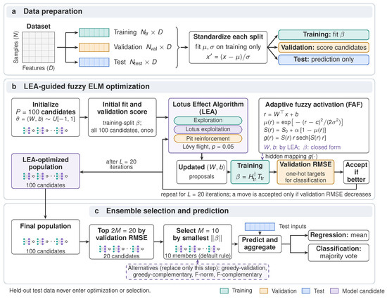
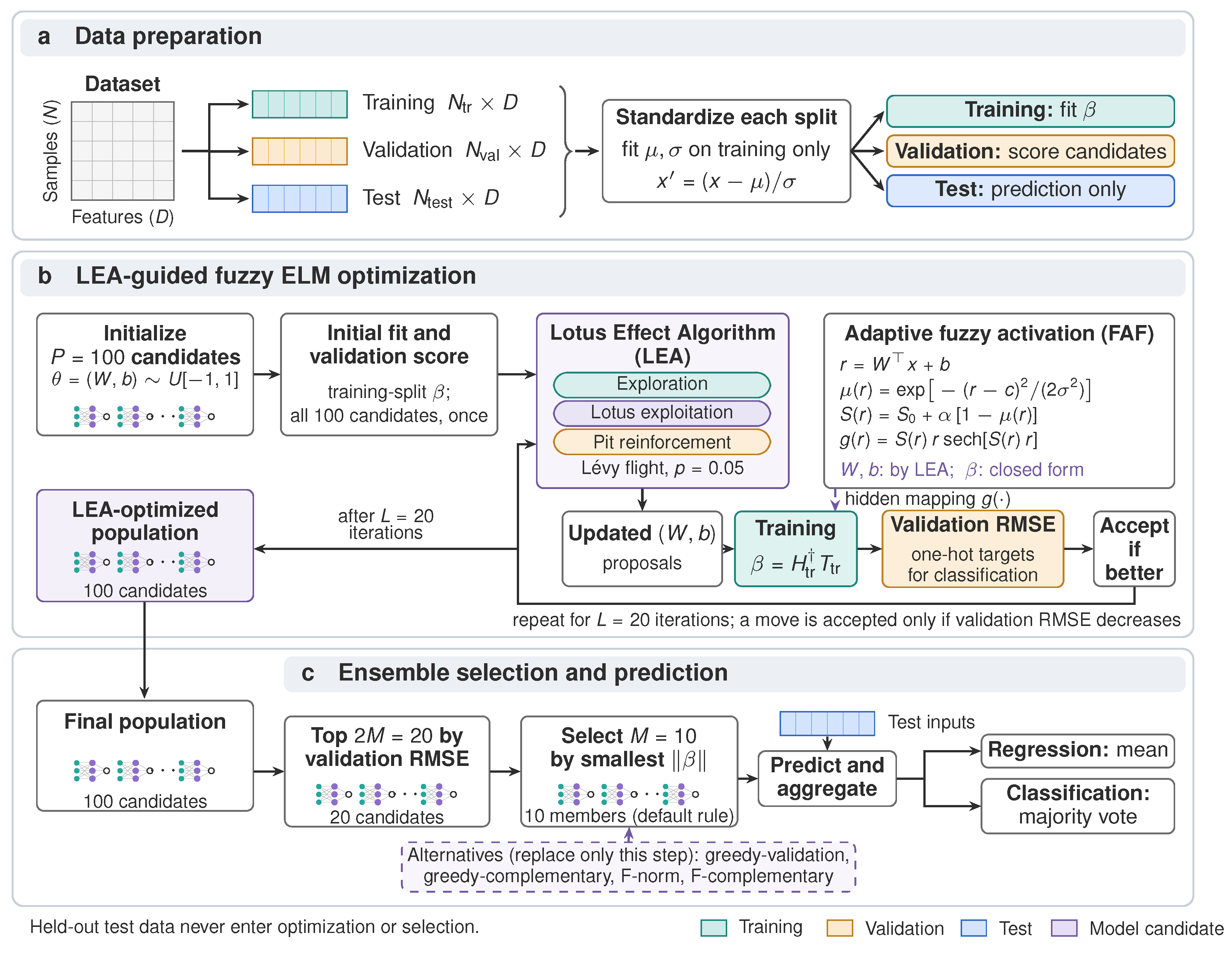
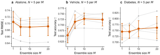
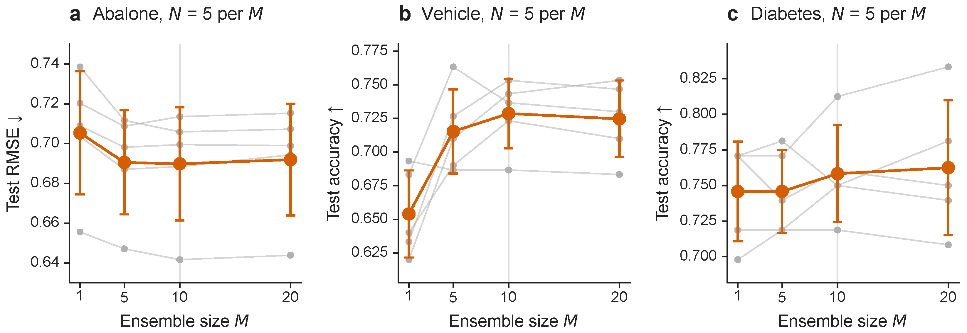
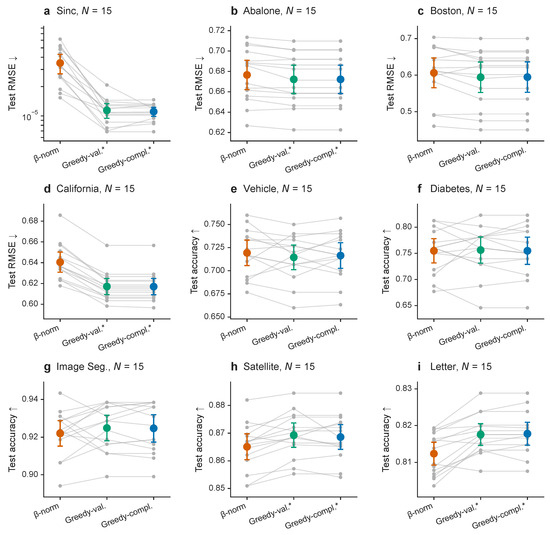
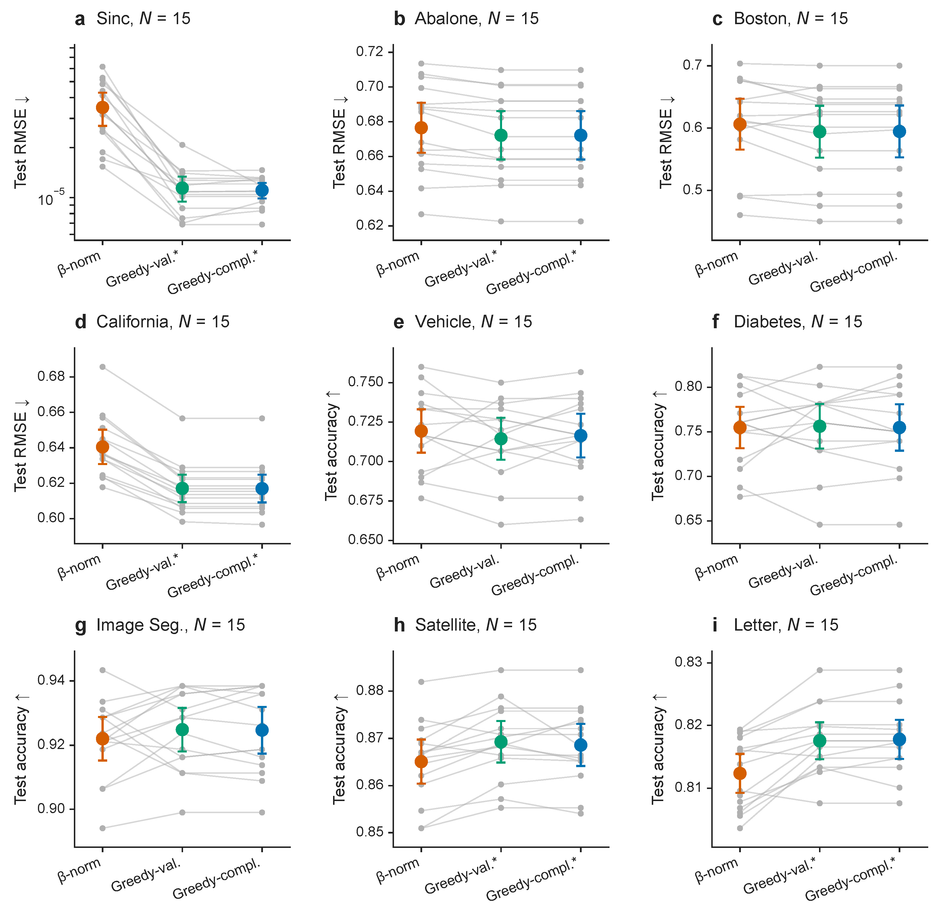
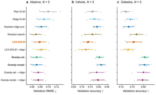
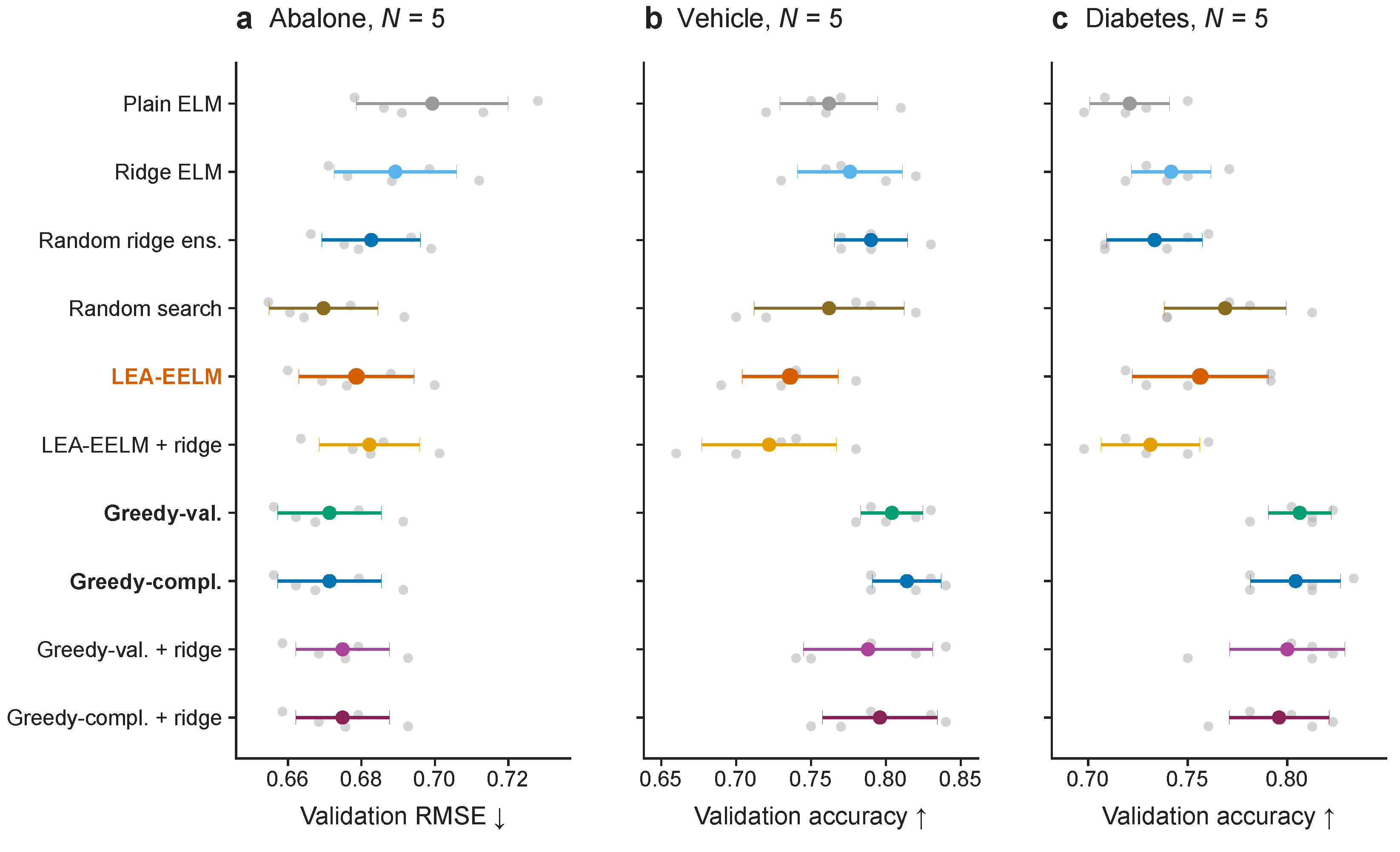
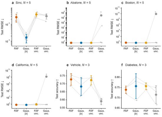
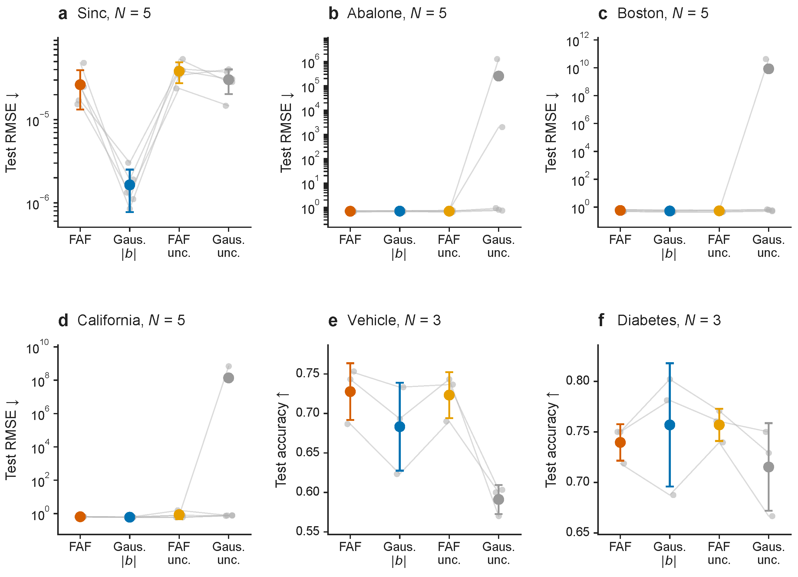
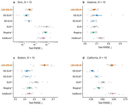
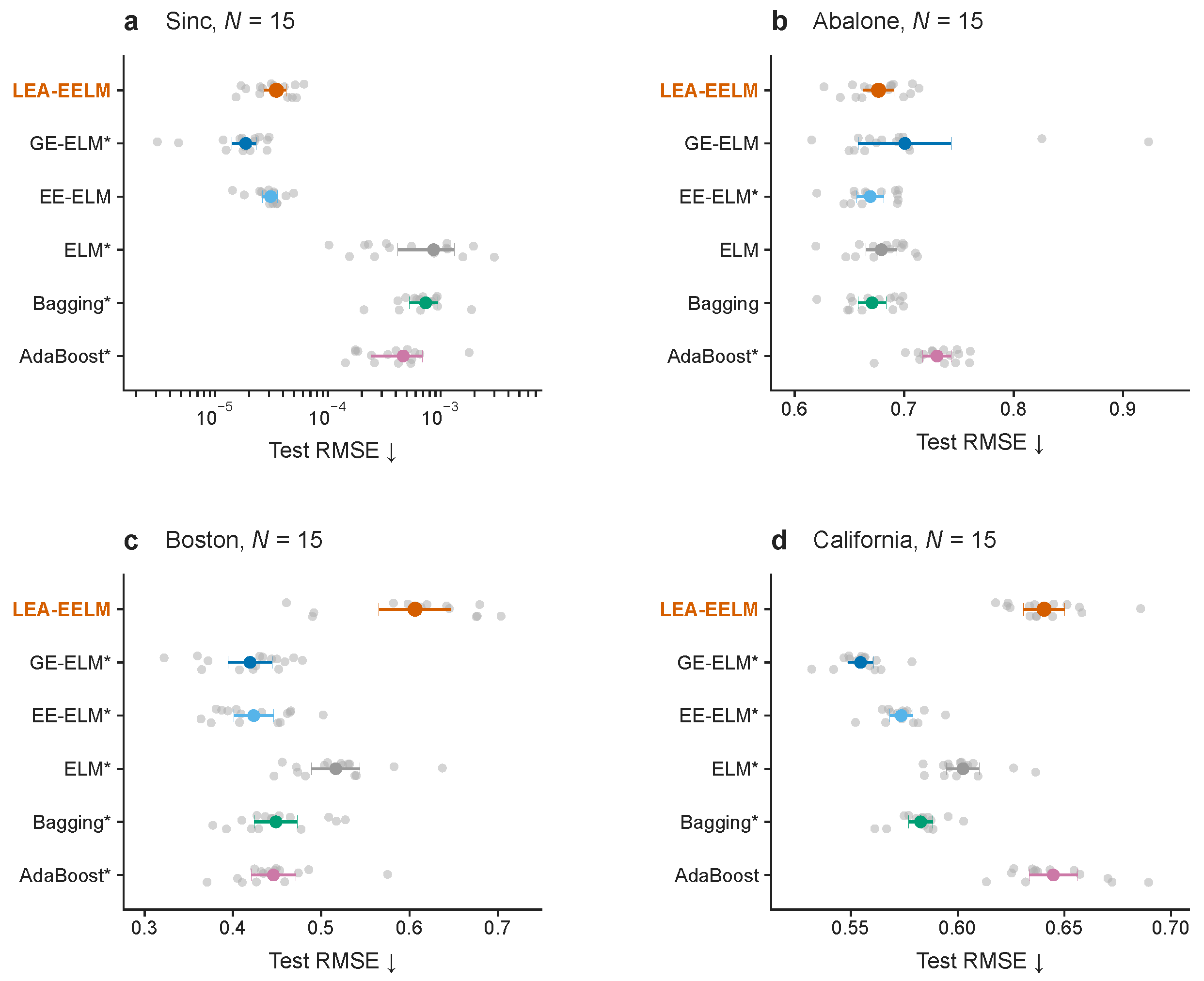
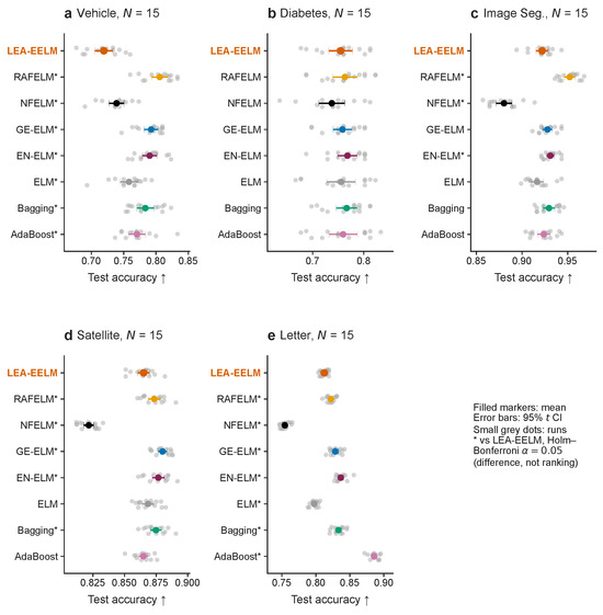
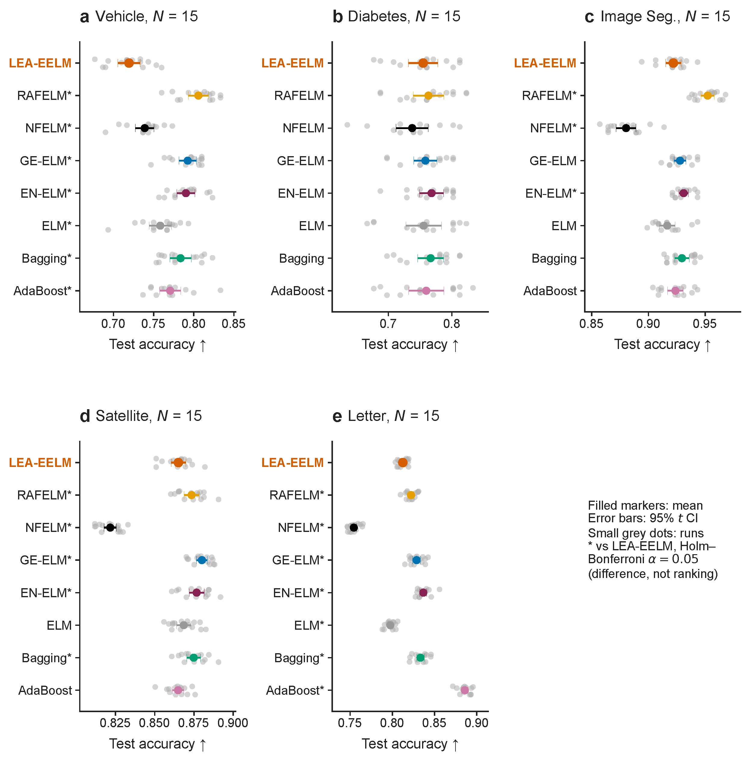

Disclaimer/Publisher’s Note: The statements, opinions and data contained in all publications are solely those of the individual author(s) and contributor(s) and not of MDPI and/or the editor(s). MDPI and/or the editor(s) disclaim responsibility for any injury to people or property resulting from any ideas, methods, instructions or products referred to in the content. |
© 2026 by the authors. Licensee MDPI, Basel, Switzerland. This article is an open access article distributed under the terms and conditions of the Creative Commons Attribution (CC BY) license.