Pell–Lucas Collocation Method for Time-Fractional Partial Integro-Differential Equations

Abstract

This paper presents a Pell–Lucas collocation method for time-fractional partial integro-differential equations (TFPIDEs) with initial and boundary conditions, where the fractional derivative is taken in the Caputo sense. The unknown solution is approximated by a truncated bivariate Pell–Lucas series, and the governing equation together with the initial and boundary conditions is discretized at uniform collocation points. Operational matrices are employed to represent the fractional-time derivative, spatial derivatives, and Volterra integral term, thereby reducing the continuous problem to a system of algebraic equations. An upper error bound in the infinity norm and a residual-based error-estimation procedure are also discussed. Numerical examples illustrate the applicability and accuracy of the proposed approach and include comparisons with exact solutions and with results reported in the literature for alternative methods.

1. Introduction

Over the past decade, partial integro-differential equations (PIDEs) have attracted increasing attention in applied sciences, including mathematics, engineering, physics, electromagnetic theory, geophysics, heat conduction, radiation propagation, poro-viscoelastic medium compression, reaction–diffusion problems, and nuclear reactor dynamics [1,2,3,4]. Because PIDEs combine integral, spatial, and temporal terms, they provide a flexible framework for modeling phenomena with memory and nonlocal effects.

The theory of partial integro-differential equations is a significant area within the study of differential and integral equations. For example, in dynamical systems with automatic control, the inclusion of an integral term in differential equations of the first and second orders is essential [5,6]. A PIDE involves partial differentiation and integration of the unknown function and is frequently employed when memory effects must be taken into account. PIDEs can be solved by a variety of methods, including finite difference schemes, collocation methods, the variational iteration method, and spline collocation methods [5,7,8].

Fractional calculus extends classical differentiation and integration to non-integer orders and has become increasingly important in science and engineering [9]. It provides a natural mathematical setting for many physical and engineering processes [10,11], and fractional differential equations have been studied extensively in the literature [12,13,14]. Because complex phenomena are often nonlocal, fractional derivatives have proved useful in modeling memory-affecting processes. Time-fractional partial integro-differential equations (TFPIDEs) have therefore received considerable attention for their ability to describe a wide range of physical, biological, financial, and control-theoretic systems [15,16,17,18,19,20,21,22,23,24]. Representative applications include viscoelastic materials, anomalous diffusion in porous media, population dynamics, delayed control systems, and asset pricing models with long-memory effects.

Since most TFPIDE problems cannot be solved exactly in closed form, numerical methods play a central role in their study. Several approaches have been proposed for fractional partial integro-differential equations, including compact finite difference methods [25,26], the homotopy analysis method [27], and variational iteration techniques [7,28]. In particular, the variational iteration method (VIM) and the homotopy perturbation method (HPM) are well-established iterative schemes for fractional integro-differential equations; they construct approximate solutions through successive corrections or homotopy expansions [7,28,29]. Additional numerical schemes for fractional PIDEs are discussed in [30,31,32]. Relative to these semi-analytical series methods and to grid-based finite-difference discretizations, spectral/collocation schemes based on polynomial operational matrices reduce the continuous TFPIDE to a single algebraic system, which is the approach taken here. The numerical treatment remains challenging because fractional operators are nonlocal, memory terms introduce long-range dependencies, and the interaction between fractional order and approximation must be handled carefully.

Although many fractional models can be formulated with alternative derivative definitions, the present work employs the classical Caputo derivative throughout. Other operators used in the recent literature include the two-scale fractal derivative [33] and related modified Caputo-type constructions in Chun-Hui He’s fractal–fractional framework [34]. We mention these alternatives briefly for context; extending the present collocation scheme to such operators is left for future work.

The present Pell–Lucas collocation scheme is conceptually related to the classical Ritz method of variational theory [35]: both seek approximate solutions in a finite-dimensional polynomial space and lead to algebraic equations for the unknown coefficients. The essential distinction is that the Ritz method arises from a variational (energy) formulation, whereas the scheme developed below is a residual collocation method driven by operational matrices for the Caputo time derivative, the spatial derivatives, and the Volterra integral term.

Related Pell–Lucas collocation studies address different equation classes. In particular, Yüzbaşı and Yıldırım applied Pell–Lucas collocation with residual correction to nonlinear population models [36] and later to a fractional HIV/AIDS compartmental system [24], while Abd-Elhameed et al. developed shifted Pell–Lucas algorithms with convergence estimates for fractional and classical Rosenau–Hyman equations [37]. Closely related spectral/collocation work for fractional PDEs includes Chebyshev–Legendre treatments of Lévy–Feller diffusion and variable-order advection–dispersion equations [38,39] and related Riesz–Feller fractional Schrödinger models [40]. The present contribution targets a linear time-fractional partial integro-differential equation with a Volterra kernel $K(x,t,s)$ and builds a unified collocation system from operational matrices for the Caputo time derivative, the spatial second derivative, and the Volterra integral term. The novelty therefore rests on this combined nonlocal treatment, not on the use of Pell–Lucas polynomials alone.

In this work, we combine Pell–Lucas (PL) polynomials with a collocation method to obtain numerical approximations of TFPIDEs with initial and boundary conditions. PL polynomials are related to Pell and Lucas numbers and have been used in number theory, combinatorics, and numerical analysis [24,41,42,43,44,45]. Their recurrence relation provides a convenient basis for constructing operational matrices of integer and fractional derivatives. Following the operational-matrix approach widely used in spectral and collocation methods [46], we approximate the solution by a truncated bivariate Pell–Lucas expansion, transform the governing equation and the Volterra integral term into matrix form, and enforce the initial and boundary conditions at uniform collocation points. This procedure reduces the original problem to a system of algebraic equations that can be treated numerically.

The main contributions of this paper are threefold: (i) the development of a Pell–Lucas collocation formulation for the TFPIDE (1) and (2); (ii) the derivation and use of operational matrices for the fractional-time derivative, spatial derivatives, and Volterra integral term, leading to an algebraic collocation system; and (iii) an error analysis comprising an upper error bound and a residual-based error-estimation procedure, together with numerical illustrations on representative test problems.

In this paper, we investigate the time-fractional partial integro-differential equation

$${}^{C}D_t^{\beta }v(x,t)=h(x,t)v_{xx}(x,t)+{\int }_0^{t}K(x,t,s)v(x,s)ds+f(x,t),a\le x\le b,0\le t\le T.$$

(1)

with the following initial and boundary conditions:

$$\begin{array}{cc}v(a,t)=q_1\left(t\right),\hfill & t\in [0,T],\hfill \\ v(b,t)=q_2\left(t\right),\hfill & t\in [0,T],\hfill \\ v(x,0)=q_3\left(x\right),\hfill & x\in [a,b],\hfill \end{array}$$

(2)

where $q_1\left(t\right),q_2\left(t\right),q_3\left(x\right)$, $h(x,t)$, and $f(x,t)$ are known continuous functions, $K(x,t,s)$ is the kernel of the Volterra integral term defined on ${\mathbb{R}}^3$, and ${}^{C}D_t^{\beta }v(x,t)$ denotes the Caputo fractional derivative of order $0<\beta \le 1$.

The approximate solution is constructed as a truncated bivariate Pell–Lucas series:

$$v(x,t)={\displaystyle \sum _{m=0}^{\infty }}{\displaystyle \sum _{s=0}^{\infty }}{a}_{m,s}{\varphi }_{m,s}(x,t),{\varphi }_{m,s}(x,t)={\varphi }_m\left(x\right){\varphi }_s\left(t\right),$$

(3)

where ${\varphi }_m\left(x\right)$ and ${\varphi }_s\left(t\right)$ are PL polynomials and $a_{m,s}$, $m,s=0,1,2,\dots$, denote the unknown coefficients.

If the infinite series (3) is truncated after $(M+1)$ terms in each variable, it can be written as

$$v(x,t)\simeq v_{2M}(x,t)={\displaystyle \sum _{m=0}^M}{\displaystyle \sum _{s=0}^M}{a}_{m,s}{\varphi }_{m,s}(x,t),m,s=0,1,2,\dots ,M.$$

(4)

Equation (1) is treated as a fractional integro-differential equation in which a Volterra integral term with a general kernel appears from the outset, rather than being obtained by converting a partial differential equation into an equivalent integral form.

The remainder of the paper is organized as follows. Section 2 reviews fractional calculus and Pell–Lucas polynomials. Section 3 derives operational matrices for integer- and fractional-order derivatives. Section 4 constructs the matrix representation of the TFPIDE together with the initial and boundary conditions. Section 5 presents the collocation system and its assembly. Section 6 discusses error bounds and error estimation. Section 7 reports numerical examples, and Section 8 gives concluding remarks.

2. Preliminaries

This section introduces the fractional operators and Pell–Lucas polynomials used throughout the paper.

2.1. Fractional Calculus

The basic notions of fractional calculus required in the subsequent analysis are reviewed below [14,15].

Definition 1.

Left-sided and right-sided Riemann–Liouville fractional integral operators $I_{a^{+}}^{\beta }$, $I_{b^{-}}^{\beta }$ where $Re\left(\beta \right)>0$ and $v\in L_1(a,b)$ are defined as:

$$I_{a^{+}}^{\beta }v\left(t\right)={\displaystyle \frac{1}{\Gamma \left(\beta \right)}}{\int }_a^t{(t-\zeta )}^{\beta -1}v\left(\zeta \right)d\zeta ,\zeta \in (a,b],t>a,$$

(5)

$$I_{b^{-}}^{\beta }v\left(t\right)={\displaystyle \frac{1}{\Gamma \left(\beta \right)}}{\int }_t^b{(\zeta -t)}^{\beta -1}v\left(\zeta \right)d\zeta ,\zeta \in [a,b),t<b,$$

(6)

Definition 2.

For $\beta >0,t>a$ and $\beta ,a,t\in \mathbb{R}$, the Caputo fractional derivative of order β, of function $v\left(t\right)$ on the interval $[a,t]$ is defined as follows:

$${}_a{}^{C}D_t^{\beta }v\left(t\right)=\left\{\begin{array}{cc}{\displaystyle \frac{1}{\Gamma (n-\beta )}}{\int }_a^t{(t-\zeta )}^{n-\beta -1}{v}^{\left(n\right)}\left(\zeta \right)d\zeta ,\hfill & n-1<\beta <n\in \mathbb{N},\hfill \\ {\displaystyle \frac{d^n}{d{t}^n}}v\left(t\right),\hfill & \beta =n\in \mathbb{N},\hfill \end{array}\right.$$

(7)

where ${}_a{}^{C}D_t^{\beta }$ represents the Caputo derivative of fractional order β.

The Caputo operator is related to the Riemann–Liouville integrals of Definition 1 by

$${}_a{}^{C}D^{\beta }v\left(t\right)=I_{a^{+}}^{n-\beta }{D}^{\left(n\right)}v\left(t\right),$$

and therefore

$${}_a{}^{C}D^{\beta }v\left(t\right)=I_{a^{+}}^{n-\beta }{v}^{\left(n\right)}\left(t\right)={\displaystyle \frac{1}{\Gamma (n-\beta )}}{\int }_a^t{(t-\zeta )}^{n-\beta -1}{v}^{\left(n\right)}\left(\zeta \right)d\zeta .$$

In particular, for $0<\beta \le 1$, the Caputo derivative of $v(x,t)$ with respect to t is defined as follows.

$${}_0{}^{C}D_t^{\beta }v(x,t)=\left\{\begin{array}{cc}{\displaystyle \frac{1}{\Gamma (1-\beta )}}{\int }_0^t{(t-s)}^{-\beta }{v}_t(x,s)ds,\hfill & 0<\beta <1,\hfill \\ v_t(x,t),\hfill & \beta =1,\hfill \end{array}\right.$$

(8)

The following properties are satisfied by fractional differential and integral operators:

$$\begin{array}{cc}\hfill & \left(1\right)I^{\beta }{I}^{\gamma }v=I^{\beta +\gamma }v,\beta ,\gamma >0,\hfill \\ \hfill & \left(2\right)I^{\beta }{t}^{\gamma }={\displaystyle \frac{\Gamma (\gamma +1)}{\Gamma (\beta +\gamma +1)}}{t}^{\beta +\gamma },\beta >0,\gamma >-1,t>0,\hfill \\ \hfill & \left(3\right)I^{\beta }{}^{C}D_t^{\beta }v\left(t\right)=v\left(t\right)-{\displaystyle \sum _{k=0}^{m-1}}{v}^{\left(k\right)}\left(0^{+}\right){\displaystyle \frac{t^k}{k!}},t>0,m-1<\beta \le m,\hfill \\ \hfill & \left(4\right){}^{C}D_t^{\beta }{I}^{\beta }v\left(t\right)=v\left(t\right),t>0,m-1<\beta \le m,\hfill \\ \hfill & \left(5\right){}^{C}D_t^{\beta }k=0,kisconstant,\hfill \\ \hfill & \left(6\right){}^{C}D_t^{\beta }{t}^{\gamma }=\left\{\begin{array}{cc}0,\hfill & \gamma \in {\mathbb{N}}_0,\gamma <\lceil \beta \rceil ,\hfill \\ {\displaystyle \frac{\Gamma (\gamma +1)}{\Gamma (\gamma -\beta +1)}}{t}^{\gamma -\beta },\hfill & \gamma \in {\mathbb{N}}_0,\gamma \ge \lceil \beta \rceil .\hfill \end{array}\right.\hfill \end{array}$$

(9)

where $\lceil \beta \rceil$ denotes the smallest integer greater than or equal to $\beta$ and ${\mathbb{N}}_0=\mathbb{N}\cup \left\{0\right\}$.

2.2. Review of the Pell–Lucas Polynomials

Polynomial bases play a central role in many applied mathematics techniques. According to the literature [47], Pell–Lucas polynomials provide effective tools for the numerical treatment of differential equations. Further properties and results can be found in [48,49].

The Pell–Lucas polynomials ${\varphi }_m\left(x\right)$ are defined by ${\varphi }_0\left(x\right)=2$, ${\varphi }_1\left(x\right)=2x$, and, for $m\ge 2$,

$${\varphi }_m\left(x\right)={\displaystyle \sum _{j=0}^{\lfloor {\displaystyle \frac{m}{2}}\rfloor }}{\displaystyle \frac{m\Gamma (m-j)}{\Gamma (j+1)\Gamma (m-2j+1)}}{\left(2x\right)}^{m-2j},$$

(10)

where $\lfloor {\displaystyle \frac{m}{2}}\rfloor$ denotes the greatest integer less than or equal to ${\displaystyle \frac{m}{2}}$. Equivalently, they satisfy the recurrence

$${\varphi }_{m+1}\left(x\right)=2x{\varphi }_m\left(x\right)+{\varphi }_{m-1}\left(x\right),m\ge 1,x\in \mathbb{R},$$

with the same initial polynomials ${\varphi }_0$ and ${\varphi }_1$ [48,49].

The derivative of ${\varphi }_m\left(x\right)$ with respect to x is defined recursively by:

$${\varphi }_m^{\prime }\left(x\right)=2x{\varphi }_{m-1}^{\prime }\left(x\right)+{\varphi }_{m-2}^{\prime }\left(x\right)+2{\varphi }_{m-1}\left(x\right),m\ge 2,$$

(11)

where ${\varphi }_0^{\prime }\left(x\right)=0$ and ${\varphi }_1^{\prime }\left(x\right)=2$.

Lemma 1.

The expansion of the following power function in the sense of PL polynomials can be expressed as follows

$$x^m={\displaystyle \frac{1}{2^m}}{\displaystyle \sum _{j=0}^{\lfloor {\displaystyle \frac{m}{2}}\rfloor }}{\displaystyle \frac{{(-1)}^j\Gamma (m+1){\zeta }_{m-2j}}{\Gamma (j+1)\Gamma (m-j+1)}}{\varphi }_{m-2j}\left(x\right),$$

(12)

where

$${\zeta }_{m-2j}=\left\{\begin{array}{cc}{\displaystyle \frac{1}{2}},\hfill & j={\displaystyle \frac{m}{2}},\hfill \\ 1,\hfill & j<{\displaystyle \frac{m}{2}}\hfill \end{array}\right..$$

(13)

Proof. 

See [50] for more details. □

Lemma 2.

The first derivative of Pell–Lucas polynomials can be written as follows.

$${\displaystyle \frac{d}{dx}}{\varphi }_m\left(x\right)=2m{\displaystyle \sum _{j=0}^{\lfloor {\displaystyle \frac{m-1}{2}}\rfloor }}{(-1)}^j{\xi }_{m-2j-1}{\varphi }_{m-2j-1}\left(x\right),m>2,$$

(14)

where the auxiliary coefficients ${\xi }_k$ are defined by

$${\xi }_k=\left\{\begin{array}{cc}{\displaystyle \frac{1}{2}},\hfill & k=0,\hfill \\ 1,\hfill & k\ge 1.\hfill \end{array}\right.$$

Proof. 

See [50]. □

The Pell–Lucas polynomial representation in Equation (10) in terms of power functions $x^j$ can be rewritten with the following formula:

$${\varphi }_m\left(x\right)=m{\displaystyle \sum _{j=0}^m}{\displaystyle \frac{2^{j+1}\Gamma \left(\frac{m+j+2}{2}\right){\delta }_{m+j}}{(m+j)\Gamma (j+1)\Gamma \left(\frac{m-j+2}{2}\right)}}{x}^j,m\ge 1,$$

(15)

where

$${\delta }_z=\left\{\begin{array}{cc}1,\hfill & zeven,\hfill \\ 0,\hfill & zodd.\hfill \end{array}\right..$$

(16)

The equivalent representation of the power function in Equation (12) in terms of Pell–Lucas polynomials is given as follows:

$$x^m={\displaystyle \frac{\Gamma (m+1)}{2^m}}{\displaystyle \sum _{j=0,(j+m)even}^m}{\displaystyle \frac{{(-1)}^{\frac{m-j}{2}}{\xi }_j}{\Gamma \left(\frac{m+j+2}{2}\right)\Gamma \left(\frac{m-j+2}{2}\right)}}{\varphi }_j\left(x\right),m\ge 1.$$

(17)

One can see [48,51] for further details on Pell–Lucas polynomials.

3. Pell–Lucas Operational Matrices

In this section, integer- and fractional-order differential operators are represented as matrix operations associated with Pell–Lucas polynomials.

3.1. Operational Matrix of Classical Derivatives

A function $v\left(x\right)\in L_2(a,b)$ can be approximated by an infinite Pell–Lucas series as follows:

$$v\left(x\right)={\displaystyle \sum _{m=0}^{\infty }}{a}_m{\varphi }_m\left(x\right).$$

(18)

where $a_m$, $m=0,1,2,\dots$, are the unknown coefficients. Truncating the series after the first $M+1$ terms, Equation (18) can be rewritten as

$$v\left(x\right)\simeq v_M\left(x\right)={\displaystyle \sum _{m=0}^M}{a}_m{\varphi }_m\left(x\right)=A^T{\Phi }_M\left(x\right),$$

(19)

where the unknown coefficients vector $A^T$ and vector of Pell–Lucas polynomials ${\Phi }_M\left(x\right)$ are defined by:

$$A^T=\left[\begin{array}{cccc}{a}_0& a_1& \cdots & a_M\end{array}\right],$$

(20)

and

$${\Phi }_M\left(x\right)={\left[\begin{array}{cccc}{\varphi }_0\left(x\right)& {\varphi }_1\left(x\right)& \cdots & {\varphi }_M\left(x\right)\end{array}\right]}^T.$$

(21)

Lemma 3.

The operational matrix of first derivative of the vector ${\Phi }_M\left(x\right)$ can be expressed as follows:

$${\displaystyle \frac{d}{dx}}{\Phi }_M\left(x\right)=W^{\left(1\right)}{\Phi }_M\left(x\right),$$

(22)

where $W^{\left(1\right)}=(w_{lm}^{\left(1\right)})$ is the operational matrix of the first derivative and has dimension $(M+1)\times (M+1)$.

Proof. 

In accordance with the property of the first order derivative of Pell–Lucas polynomials, the elements of matrix $W^{\left(1\right)}$ are represented as follows:

$$w_{lm}^{\left(1\right)}=\left\{\begin{array}{cc}2l{(-1)}^{{\displaystyle \frac{l-m+1}{2}}}{\xi }_m,\hfill & l>m,(l+m)odd,\hfill \\ 0,\hfill & l\le m,(l+m)even.\hfill \end{array}\right.$$

(23)

The Pell–Lucas operational matrix of the nth-order derivative of the vector ${\Phi }_M\left(x\right)$ can be expressed as

$${\displaystyle \frac{d^n}{d{x}^n}}{\Phi }_M\left(x\right)=W^{\left(n\right)}{\Phi }_M\left(x\right)={\left(W^{\left(1\right)}\right)}^n{\Phi }_M\left(x\right),$$

(24)

where $n\in {\mathbb{Z}}^{+}$. For further details, see [49]. □

3.2. Operational Matrix of Derivative of Fractional Order

Theorem 1.

Assume ${\Phi }_M\left(x\right)$ is the Pell–Lucas vector defined in Equation (21). The Caputo fractional derivative of order β of ${\Phi }_M\left(x\right)$ can be represented as follows:

$${}^{C}D_x^{\beta }{\Phi }_M\left(x\right)=x^{-\beta }{H}^{\left(\beta \right)}{\Phi }_M\left(x\right),$$

(25)

where $H^{\left(\beta \right)}=(h_{p,l}^{\beta })$ is an $(M+1)\times (M+1)$ matrix representing the Pell–Lucas operational matrix of the Caputo derivative of order β and can be expressed as follows:

$$H^{\left(\beta \right)}=\left(\begin{array}{ccccc}0& 0& 0& \cdots & 0\\ ⋮& ⋮& ⋮& & ⋮\\ {\zeta }_{\beta }(\lceil \beta \rceil ,0)& {\zeta }_{\beta }(\lceil \beta \rceil ,1)& 0& \cdots & 0\\ ⋮& ⋮& ⋮& & ⋮\\ {\zeta }_{\beta }(p,0)& \cdots & {\zeta }_{\beta }(p,p)& \cdots & 0\\ ⋮& ⋮& ⋮& & ⋮\\ {\zeta }_{\beta }(M,0)& {\zeta }_{\beta }(M,1)& {\zeta }_{\beta }(M,2)& \cdots & {\zeta }_{\beta }(M,M)\end{array}\right),$$

(26)

where the elements of $H^{\left(\beta \right)}$ can be given as

$$h_{p,l}^{\beta }=\left\{\begin{array}{cc}{\zeta }_{\beta }(p,l),\hfill & p\ge l,p\ge \lceil \beta \rceil ,l=0,1,\dots ,p,\hfill \\ 0,\hfill & p<l,p<\lceil \beta \rceil ,\hfill \end{array}\right.$$

(27)

where

$${\zeta }_{\beta }(p,l)=p{\displaystyle \sum _{n=\lceil \beta \rceil ,n-l+2>0}^p}{\displaystyle \frac{{(-1)}^{\frac{n-l}{2}}{\delta }_{p+n}{\delta }_{l+n}{\xi }_l\Gamma (n+1)\Gamma \left(\frac{p+n}{2}\right)}{\Gamma \left(\frac{p-n+2}{2}\right)\Gamma \left(\frac{n-l+2}{2}\right)\Gamma \left(\frac{n+l+2}{2}\right)\Gamma (n-\beta +1)}}.$$

(28)

Proof. 

Using the Pell–Lucas polynomials definition in Equation (15) and definition of ${\delta }_z$ in Equation (16). The power function $x^m$ can be represented as:

$$x^m={\displaystyle \frac{\Gamma (m+1)}{2^m}}{\displaystyle \sum _{j=0}^m}{\displaystyle \frac{{(-1)}^{\frac{m-j}{2}}{\xi }_j{\delta }_{j+m}}{\Gamma \left(\frac{m+j+2}{2}\right)\Gamma \left(\frac{m-j+2}{2}\right)}}{\varphi }_j\left(x\right),m\ge 1.$$

(29)

By calculating the fractional derivative of ${\varphi }_p\left(x\right)$ in the Caputo sense of order $\beta$ of Equation (21) is defined as follows:

$${}^{C}D_x^{\beta }{\varphi }_p\left(x\right)={\displaystyle \sum _{j=0}^p}{\displaystyle \frac{2^{j+1}\Gamma (\frac{p+j+2}{2}){\delta }_{p+j}}{(j+p)\Gamma (j+1)\Gamma (\frac{p-j+1}{2})}}{}^{C}D_x^{\beta }{x}^j.$$

(30)

Now, using Equation (7), we write Equation (30) for values greater than $\lceil \beta \rceil$ as follows:

$${}^{C}D_x^{\beta }{\varphi }_p\left(x\right)=p{x}^{-\beta }{\displaystyle \sum _{j=\lceil \beta \rceil }^p}{\displaystyle \frac{2^{j+1}\Gamma (\frac{p+j+2}{2}){\delta }_{p+j}}{(j+p)\Gamma (\frac{p-j+1}{2})\Gamma (j-\beta +1)}}{x}^j.$$

(31)

By changing the index from j to n, we have

$${}^{C}D_x^{\beta }{\varphi }_p\left(x\right)=p{x}^{-\beta }{\displaystyle \sum _{n=\lceil \beta \rceil }^p}{\displaystyle \frac{2^{n+1}\Gamma \left(\frac{p+n+2}{2}\right){\delta }_{p+n}}{(p+n)\Gamma \left(\frac{p-n+2}{2}\right)\Gamma (n-\beta +1)}}{x}^n.$$

(32)

By replacing $x^n$ of Equation (29) in Equation (32) and using the properties of the Gamma function, we will have

$${}^{C}D_x^{\beta }{\varphi }_p\left(x\right)=x^{-\beta }{\displaystyle \sum _{\begin{array}{c}l=0\\ n-l+2>0\end{array}}^p}\left(p{\displaystyle \sum _{n=\lceil \beta \rceil }^p}{\displaystyle \frac{{(-1)}^{\frac{n-l}{2}}{\delta }_{p+n}{\delta }_{l+n}{\zeta }_l\Gamma (n+1)\Gamma \left(\frac{p+n}{2}\right)}{\Gamma \left(\frac{p-n+2}{2}\right)\Gamma \left(\frac{n+l+2}{2}\right)\Gamma \left(\frac{n-l+2}{2}\right)\Gamma (n-\beta +1)}}\right){\varphi }_l\left(x\right),$$

(33)

then Equation (33) can be written as:

$${}^{C}D_x^{\beta }{\varphi }_p\left(x\right)=x^{-\beta }{\displaystyle \sum _{l=0}^p}{\zeta }_{\beta }(p,l){\varphi }_l\left(x\right),$$

(34)

where ${\zeta }_{\beta }(p,l)$ is given in Equation (28).

Equation (34) can also be expressed as the vector form

$${}^{C}D_x^{\beta }{\varphi }_p\left(x\right)=x^{-\beta }[{\zeta }_{\beta }(p,0),{\zeta }_{\beta }(p,1),\dots ,{\zeta }_{\beta }(p,p),0,0,\dots ,0]\Phi \left(x\right),\lceil \beta \rceil \le j\le N,$$

(35)

Moreover, we can write

$${}^{C}D_x^{\beta }{\varphi }_p\left(x\right)=x^{-\beta }[0,0,\dots ,0],0\le p\le \lceil \beta \rceil -1.$$

(36)

Combining Equations (35) and (36) yields the desired result. □

4. Matrix Representations

To obtain a matrix formulation of Equation (1) in terms of Pell–Lucas polynomials, we rewrite it as

$$D_1(x,t)-D_2(x,t)=f(x,t),$$

(37)

where the derivative and integral parts are expressed as follows:

$$D_1(x,t)={}^{C}D_t^{\beta }v(x,t)-h(x,t)v_{xx}(x,t),$$

(38)

and

$$D_2(x,t)={\int }_0^{t}K(x,t,s)v(x,s)ds.$$

(39)

The problem is thereby transformed into a system of algebraic equations, and the approximate solution is obtained by the collocation method described below.

Lemma 4.

The approximate solution (3) in terms of Pell–Lucas polynomials can be represented as:

$$v_{2M}(x,t)={\Phi }_M\left(x\right){\overline{\Phi }}_M\left(t\right){\overline{\mathit{A}}}_M,$$

(40)

where

$${\overline{\mathit{A}}}_M={[{\mathit{A}}_0,{\mathit{A}}_1,\dots ,{\mathit{A}}_M]}^T,{\mathit{A}}_i={[a_{i,0},a_{i,1},\dots ,a_{i,M}]}^T,i=0,1,2,\dots ,M,$$

$${\Phi }_M\left(x\right)=[{\varphi }_0\left(x\right),{\varphi }_1\left(x\right),\dots ,{\varphi }_M\left(x\right)],$$

and ${\overline{\Phi }}_M\left(t\right)=diag\left({\Phi }_M\left(t\right)\right)$.

Proof. 

The expansion of approximate solution $v_{2M}(x,t)$ with respect to Pell–Lucas vectors ${\Phi }_M\left(x\right)$ and ${\Phi }_M\left(t\right)$ can be easily expressed by Equation (40). □

Lemma 5.

The second-order spatial partial derivative of Equation (3) in terms of PL polynomials in matrix structure can be represented by:

$${\left(v_{2M}(x,t)\right)}_{xx}={\Phi }_M\left(x\right){\mathit{N}}^2{\overline{\Phi }}_M\left(t\right){\overline{\mathit{A}}}_M,$$

(41)

where if M is odd

$$\mathit{N}={\left(\begin{array}{cccccc}0& 1& 0& -3& \cdots & {(-1)}^{{\displaystyle \frac{M-1}{2}}}M\\ 0& 0& 4& 0& \cdots & 0\\ 0& 0& 0& 6& \cdots & {(-1)}^{{\displaystyle \frac{M-3}{2}}}2M\\ ⋮& ⋮& ⋮& ⋮& \ddots & 2M\\ 0& 0& 0& 0& \cdots & 0\end{array}\right)}_{(M+1)\times (M+1)},$$

and if M is even

$$\mathit{N}={\left(\begin{array}{cccccc}0& 1& 0& -3& \cdots & 0\\ 0& 0& 4& 0& \cdots & {(-1)}^{{\displaystyle \frac{M-2}{2}}}2M\\ 0& 0& 0& 6& \cdots & 0\\ ⋮& ⋮& ⋮& ⋮& \ddots & ⋮\\ 0& 0& 0& 0& \cdots & 0\end{array}\right)}_{(M+1)\times (M+1)},$$

where, ${\Phi }_M\left(x\right),{\overline{\Phi }}_M\left(t\right)$ and ${\overline{\mathit{A}}}_M$ are defined in Lemma 4. The two displays represent the same truncated differentiation map ${\Phi }_M\mapsto {\Phi }_M^{\prime }$ (and thence ${\Phi }_M^{″}={\Phi }_M{\mathbf{N}}^2$); the even/odd cases differ only in which entries of the highest-degree columns remain nonzero after truncation of the Pell–Lucas derivative recurrence.

Proof. 

The first and second spatial derivatives of approximate solution in Equation (40) in matrix form can be expressed as follows:

$${\left(v_{2M}(x,t)\right)}_x={\Phi }_M^{\prime }\left(x\right){\overline{\Phi }}_M\left(t\right){\overline{\mathbf{A}}}_M,$$

(42)

and

$${\left(v_{2M}(x,t)\right)}_{xx}={\Phi }_M^{″}\left(x\right){\overline{\Phi }}_M\left(t\right){\overline{\mathbf{A}}}_M,$$

(43)

In order to construct the matrix structure of ${\Phi }_M^{″}\left(x\right)$ in Equation (43), we use the recurrence formula of first derivative of Pell–Lucas polynomials. So, the matrix structure of the second derivative of ${\Phi }_M\left(x\right)$ can be written as:

$${\Phi }_M^{″}\left(x\right)={\Phi }_M\left(x\right){\mathbf{N}}^2.$$

(44)

Finally, by substituting Equation (44) into the expression (43), the matrix structure (41) is derived. The parity dependence of the displayed pattern of $\mathbf{N}$ arises because the highest retained index generated by the derivative recurrence depends on whether the truncation degree M is even or odd; both forms encode the same linear map on the truncated basis. □

Lemma 6.

The matrix structure of $K(x,t,s)$ in Equation (39) can be represented in terms of PL polynomials as follows:

$$\left[K(x,t,s)\right]={\mathit{X}}_M\left(x\right){\overline{\mathit{X}}}_M\left(t\right)\mathit{K}{\mathit{X}}_M^T\left(s\right),\mathit{K}=\left[k_{p_1,p_2,p_3}^T\right],p_1,p_2,p_3=0,1,\dots ,M,$$

(45)

where

$$k_{p_1,p_2,p_3}^T={\displaystyle \frac{1}{p_1!p_2!p_3!}}{\displaystyle \frac{{\partial }^{p_1+p_2+p_3}K(0,0,0)}{\partial x^{p_1}\partial t^{p_2}\partial s^{p_3}}},p_1,p_2,p_3=0,1,\dots ,M,$$

(46)

$${\mathit{X}}_M\left(x\right)=\left[\begin{array}{cccc}1& x& \cdots & x^M\end{array}\right],{\mathit{X}}_M^T\left(s\right)={\left[\begin{array}{cccc}1& s& \cdots & s^M\end{array}\right]}^T,{\overline{\mathit{X}}}_M\left(t\right)=diag\left({\mathit{X}}_M\left(t\right)\right).$$

Proof. 

The kernel $K(x,t,s)$ based on the truncated Maclaurin series, can be expressed as follows:

$$K(x,t,s)={\displaystyle \sum _{p_1=0}^M}{\displaystyle \sum _{p_2=0}^M}{\displaystyle \sum _{p_3=0}^M}{k}_{p_1,p_2,p_3}^T{x}^{p_1}{t}^{p_2}{s}^{p_3}.$$

(47)

Multiplying by $\mathbf{K}{\mathbf{X}}_M^T\left(x\right)$, from the right side in vector ${\mathbf{X}}_M\left(x\right){\overline{\mathbf{X}}}_M\left(t\right)$, the relation (45) is obtained. □

In the collocation scheme, the Volterra integral term is therefore not evaluated by numerical quadrature of the original kernel at each step. Instead, after truncating K by its Maclaurin polynomial, the integral against the Pell–Lucas expansion of $v_{2M}$ is converted into an exact matrix product through the operational representation of Lemma 7 (and the associated integrated basis factors).

Lemma 7.

In the Volterra integral Equation (39), the expression $v_{2M}(x,s)$ has the following matrix representation:

$$v_{2M}(x,s)={\Phi }_M\left(s\right){\overline{\Phi }}_M\left(x\right){\overline{\mathit{A}}}_M^{\ast },$$

(48)

where

$${\overline{\mathit{A}}}_M^{\ast }={\left[\begin{array}{cccc}{\mathit{A}}_0^{\ast }& {\mathit{A}}_1^{\ast }& \cdots & {\mathit{A}}_M^{\ast }\end{array}\right]}^T,{\mathit{A}}_i^{\ast }={\left[\begin{array}{cccc}{a}_{0,i}& a_{1,i}& \cdots & a_{M,i}\end{array}\right]}^T,$$

$${\Phi }_M\left(s\right)=\left[\begin{array}{cccc}{\varphi }_0\left(s\right)& {\varphi }_1\left(s\right)& \cdots & {\varphi }_M\left(s\right)\end{array}\right],{\overline{\Phi }}_M\left(x\right)=diag\left({\Phi }_M\left(x\right)\right).$$

Proof. 

By substituting s instead of t in Lemma 4, we have

$$v_{2M}(x,s)={\Phi }_M\left(x\right){\overline{\Phi }}_M\left(s\right){\overline{\mathbf{A}}}_M.$$

(49)

This expression can be more exactly written as follows:

$$v_{2M}(x,s)=\left[a_{0,0}s{a}_{0,1}{s}^2{a}_{0,2}x{a}_{1,0}xs{a}_{1,1}x{s}^2{a}_{1,2}{x}^2{a}_{2,0}{x}^{2}s{a}_{2,1}{x}^2{s}^2{a}_{2,2}\right]$$

(50)

If ${\Phi }_M\left(s\right)$ and ${\overline{\Phi }}_M\left(x\right)$ are substituted in place of ${\Phi }_M\left(x\right)$ and ${\overline{\Phi }}_M\left(s\right)$ in Equation (49), then ${\overline{\mathbf{A}}}_M^{\ast }$ is written instead of ${\overline{\mathbf{A}}}_M$ to obtain the equality in Equation (50). Consequently, Equation (48) is obtained.

Explicitly, both stacked vectors have length ${(M+1)}^2$ and contain the same scalars $a_{i,j}$. Writing

$${\overline{\mathbf{A}}}_M={\left(a_{0,0},\dots ,a_{0,M},a_{1,0},\dots ,a_{1,M},\dots ,a_{M,0},\dots ,a_{M,M}\right)}^T$$

(spatial index outer) and

$${\overline{\mathbf{A}}}_M^{\ast }={\left(a_{0,0},\dots ,a_{M,0},a_{0,1},\dots ,a_{M,1},\dots ,a_{0,M},\dots ,a_{M,M}\right)}^T$$

(temporal index outer), one has the exact identity

$${\overline{\mathbf{A}}}_M^{\ast }=P{\overline{\mathbf{A}}}_M,$$

(51)

where $P\in {\mathbb{R}}^{N\times N}$ with $N={(M+1)}^2$ is the (symmetric involutory) commutation matrix defined by

$$P{e}_{i(M+1)+j}=e_{j(M+1)+i},i,j=0,\dots ,M$$

(equivalently, if $A=\left(a_{i,j}\right)$ then ${\overline{\mathbf{A}}}_M=\mathrm{vec}\left(A\right)$ and ${\overline{\mathbf{A}}}_M^{\ast }=\mathrm{vec}\left(A^T\right)$ in row-major stacking). Thus P has dimension ${(M+1)}^2\times {(M+1)}^2$. In particular $P=P^T=P^{-1}$, and ${\overline{\mathbf{A}}}_M^{\ast }$ does not introduce independent unknowns: every occurrence of ${\overline{\mathbf{A}}}_M^{\ast }$ in Lemmas 8 and 9 is the same coefficient vector as ${\overline{\mathbf{A}}}_M$, only reordered for the Volterra/time layout. □

Lemma 8.

The matrix representation of time-fractional derivative of order β of Equation (3) in Caputo sense has the following matrix structure:

$${}^{C}D_t^{\beta }{v}_{2M}(x,t)=t^{-\beta }{\Phi }_M\left(t\right){\left(H^{\left(\beta \right)}\right)}^T{\overline{\Phi }}_M\left(x\right){\overline{\mathit{A}}}_M^{\ast },$$

(52)

Here, ${\Phi }_M\left(t\right),{\overline{\Phi }}_M\left(x\right)$ and ${\overline{\mathit{A}}}_M^{\ast }$ are as in Lemma 7, and $H^{\left(\beta \right)}$ in Equation (26).

Proof. 

By taking the Caputo fractional derivative of order $\beta$ of the approximate solution (48) with respect to t, we obtain

$${}^{C}D_t^{\beta }{v}_{2M}(x,t)={}^{C}D_t^{\beta }\left({\Phi }_M\left(t\right){\overline{\Phi }}_M\left(x\right){\overline{\mathbf{A}}}_M^{\ast }\right),$$

(53)

then, ${}^{C}D_t^{\beta }{\Phi }_M\left(t\right)$ in Equation (53) in matrix form can be represented as $t^{-\beta }{\Phi }_M\left(t\right){\left(H^{\left(\beta \right)}\right)}^T$ based on Equation (25). Inserting this relationship into Equation (53) gives the desired result. □

Lemma 9.

The term $D_1(x,t)$ has the following matrix structure:

$$\left[D_1(x,t)\right]=t^{-\beta }{\Phi }_M\left(t\right){\left(H^{\left(\beta \right)}\right)}^T{\overline{\Phi }}_M\left(x\right){\overline{\mathit{A}}}_M^{\ast }-\left[h(x,t)\right]{\Phi }_M\left(x\right){\mathit{N}}^2{\overline{\Phi }}_M\left(t\right){\overline{\mathit{A}}}_M.$$

(54)

Here, ${\Phi }_M\left(t\right),{\overline{\Phi }}_M\left(x\right)$ and ${\overline{\mathit{A}}}_M^{\ast }$ are as in Lemma 8, ${\Phi }_M\left(x\right),{\overline{\Phi }}_M\left(t\right)$ and ${\overline{\mathit{A}}}_M$ are as in Theorem 4 and $\mathit{N}$ in Lemma 5.

Proof. 

By substituting Equations (41) and (52) into Equation (38), the desired result is obtained. □

Lemma 10.

The matrix representation of $D_2(x,t)$ in Equation (38) can be expressed as

$$\left[D_2(x,t)\right]={\mathit{X}}_M\left(x\right){\overline{\mathit{X}}}_M\left(t\right)\mathit{K}\mathit{S}\left(t\right){\overline{\Phi }}_M\left(x\right){\overline{\mathit{A}}}_M^{\ast },$$

(55)

where

$$\mathit{S}\left(t\right)={\int }_0^t{\mathit{X}}_M^T\left(s\right){\Phi }_M\left(s\right)ds.$$

Here, ${\mathit{X}}_M\left(x\right),{\overline{\mathit{X}}}_M\left(t\right),\mathit{K}$ and ${\mathit{X}}_M^T\left(s\right)$ are in Lemma 6 and ${\Phi }_M\left(s\right),{\overline{\Phi }}_M\left(x\right),{\overline{\mathit{A}}}_M^{\ast }$ are in Lemma 7.

Proof. 

By employing Equations (45) and (48) into Equation (39), the matrix form of $D_2(x,t)$ can be easily obtained. □

In the following, the initial and boundary conditions (2) are written in matrix form.

Lemma 11.

The matrix form of the conditions (2) is given by

$$\begin{array}{c}{\Phi }_M\left(a\right){\overline{\Phi }}_M\left(t\right){\overline{\mathit{A}}}_M=q_1\left(t\right),\hfill \\ {\Phi }_M\left(b\right){\overline{\Phi }}_M\left(t\right){\overline{\mathit{A}}}_M=q_2\left(t\right),\hfill \\ {\Phi }_M\left(x\right){\overline{\Phi }}_M\left(0\right){\overline{\mathit{A}}}_M=q_3\left(x\right).\hfill \end{array}$$

(56)

Here, ${\Phi }_M\left(x\right),{\overline{\Phi }}_M\left(t\right)$ and ${\overline{\mathit{A}}}_M$ are as in Lemma 4.

Proof. 

By inserting $a,b$ instead of x and 0 instead of t in Lemma 4, we obtain $v_{2M}(a,t)={\Phi }_M\left(a\right){\overline{\Phi }}_M\left(t\right){\overline{\mathbf{A}}}_M$, $v_{2M}(b,t)={\Phi }_M\left(b\right){\overline{\Phi }}_M\left(t\right){\overline{\mathbf{A}}}_M$ and $v_{2M}(x,0)={\Phi }_M\left(x\right){\overline{\Phi }}_M\left(0\right){\overline{\mathbf{A}}}_M$, respectively. By using Equation (2), the desired result is easily obtained. □

5. Procedure of the Solution

This section describes the Pell–Lucas collocation method on uniform collocation points. The operational matrices derived in the previous sections are used to assemble a linear algebraic system for the unknown expansion coefficients.

The truncated series expansion (3) is substituted into Equation (1) and into the initial and boundary conditions (2). Using the matrix representations of the fractional-time derivative, spatial derivatives, and Volterra integral term, the governing equation can be written as

$$\begin{array}{c}\left\{t^{-\beta }{\Phi }_M\left(t\right){\left(H^{\left(\beta \right)}\right)}^T{\overline{\Phi }}_M\left(x\right)-{\mathbf{X}}_M\left(x\right){\overline{\mathbf{X}}}_M\left(t\right)\mathbf{K}\mathbf{S}\left(t\right){\overline{\Phi }}_M\left(x\right)\right\}{\overline{\mathbf{A}}}_M^{\ast }\hfill \\ -\left[h(x,t)\right]\left\{{\Phi }_M\left(x\right){\mathbf{N}}^2{\overline{\Phi }}_M\left(t\right)\right\}{\overline{\mathbf{A}}}_M=\left[f(x,t)\right].\hfill \end{array}$$

We define uniformly spaced collocation points by

$$x_i=a+{\displaystyle \frac{b-a}{M}}i,i=0,1,\dots ,M,t_j={\displaystyle \frac{T}{M}}j,j=0,1,\dots ,M.$$

(57)

We assume that the matrix representation for the approximate solution of Equations (1) and (2) is as follows:

$${\mathbf{Z}}^{\ast }{\overline{\mathbf{A}}}_M^{\ast }-\mathbf{Z}{\overline{\mathbf{A}}}_M=\mathbf{F}.$$

(58)

Using the structure of ${\overline{\mathbf{A}}}_M$ and ${\overline{\mathbf{A}}}_M^{\ast }$, Equation (58) may be recast as a linear system in the coefficients of ${\overline{\mathbf{A}}}_M$. Substituting the collocation points (57) into (58) yields the algebraic system

$${\mathbf{Z}}^{\ast }(x_i,t_j){\overline{\mathbf{A}}}_M^{\ast }-\mathbf{Z}(x_i,t_j){\overline{\mathbf{A}}}_M=\left[f(x_i,t_j)\right],$$

(59)

where

$${\mathbf{Z}}^{\ast }=\left(\begin{array}{c}{\mathbf{Z}}_0^{\ast }\\ {\mathbf{Z}}_1^{\ast }\\ ⋮\\ {\mathbf{Z}}_M^{\ast }\end{array}\right),{\mathbf{Z}}_i^{\ast }=\left(\begin{array}{c}{\mathbf{Z}}^{\ast }(x_i,t_0)\\ {\mathbf{Z}}^{\ast }(x_i,t_1)\\ ⋮\\ {\mathbf{Z}}^{\ast }(x_i,t_M)\end{array}\right),\mathbf{Z}=\left(\begin{array}{c}{\mathbf{Z}}_0\\ {\mathbf{Z}}_1\\ ⋮\\ {\mathbf{Z}}_M\end{array}\right),{\mathbf{Z}}_i=\left(\begin{array}{c}\mathbf{Z}(x_i,t_0)\\ \mathbf{Z}(x_i,t_1)\\ ⋮\\ \mathbf{Z}(x_i,t_M)\end{array}\right),$$

(60)

and

$$\mathbf{F}=\left(\begin{array}{c}{\mathbf{F}}_0\\ {\mathbf{F}}_1\\ ⋮\\ {\mathbf{F}}_M\end{array}\right),{\mathbf{F}}_j=\left(\begin{array}{c}f(x_j,t_0)\\ f(x_j,t_1)\\ ⋮\\ f(x_j,t_M)\end{array}\right),j=0,1,\dots ,M.$$

(61)

Lemma 12.

The initial and boundary conditions (2) in collocation points (57) can be represented as follows:

$$\mathit{U}{\overline{\mathit{A}}}_M={\eta }_j,\mathit{V}{\overline{\mathit{A}}}_M={\vartheta }_j,\mathit{W}{\overline{\mathit{A}}}_M={\delta }_i,$$

(62)

where

$$\mathit{U}=\left(\begin{array}{c}{\mathit{U}}_0\\ {\mathit{U}}_1\\ ⋮\\ {\mathit{U}}_M\end{array}\right),\mathit{V}=\left(\begin{array}{c}{\mathit{V}}_0\\ {\mathit{V}}_1\\ ⋮\\ {\mathit{V}}_M\end{array}\right),\mathit{W}=\left(\begin{array}{c}{\mathit{W}}_0\\ {\mathit{W}}_1\\ ⋮\\ {\mathit{W}}_M\end{array}\right),{\delta }_i=\left(\begin{array}{c}{w}_{j,1}{w}_{j,2}\dots w_{j,{(M+1)}^2}\end{array}\right),$$

$${\eta }_j=\left(\begin{array}{c}{u}_{j,1}{u}_{j,2}\dots u_{j,{(M+1)}^2}\end{array}\right),{\vartheta }_j=\left(\begin{array}{c}{v}_{j,1}{v}_{j,2}\dots v_{j,{(M+1)}^2}\end{array}\right),$$

$${\mathit{U}}_j={\Phi }_M\left(a\right){\overline{\Phi }}_M\left(t_j\right),{\mathit{V}}_j={\Phi }_M\left(b\right){\overline{\Phi }}_M\left(t_j\right),{\mathit{W}}_i={\Phi }_M\left(x_i\right){\overline{\Phi }}_M\left(0\right).$$

Proof. 

The stated block rows follow by evaluating the matrix forms of the initial and boundary conditions in Lemma 11 at the collocation nodes (57). □

The condition number of the collocation algebraic system in Equation (59) grows rapidly with M; for Example 1 with $\beta =0.55$ and $M=6$, the unscaled matrix condition number is already large (of order ${10}^8$–${10}^{18}$, depending on whether the overdetermined matrix or the normal equations are monitored). Adding Equation (62) to the system (59) yields the generalized matrix system

$$[{\tilde{\mathbf{Z}}}^{\ast };\tilde{\mathbf{Z}};\tilde{\mathbf{F}}].$$

(63)

Solving the system (63) yields the Pell–Lucas coefficient vector ${\overline{\mathbf{A}}}_M$, and the approximate solution is obtained by substituting these coefficients into Equation (3).

6. Error Analysis

This section presents an upper bound for the approximation error and a residual-based error-estimation procedure for the Pell–Lucas collocation method. The first result provides an error bound in the infinity norm, and the second characterizes the error through an auxiliary problem that can be used when an exact solution is unavailable.

Lemma 13

(Upper Bound of Error). Let v denote the exact solution of Equation (1), and let $v_{2M}$ denote its Pell–Lucas polynomial approximation on the domain $[a,b]\times [0,T]$. Let $v_{2M}^{Mac}$ be the truncated Maclaurin series of the exact solution $v(x,t)$ in the domain $[a,b]\times [0,T]$. The absolute error of the proposed method has an upper bound as follows:

$${\parallel v-v_{2M}\parallel }_{\infty }\le k_M{\parallel {\widetilde{\tilde{\mathit{A}}}}_M\parallel }_{\infty }+{\mathit{q}}_M{\overline{\mathit{q}}}_M{\parallel {\overline{\mathit{A}}}_M\parallel }_{\infty }$$

$$+{\displaystyle \frac{1}{(2M+1)!}}{\parallel {\left(x{\displaystyle \frac{\partial }{\partial x}}+t{\displaystyle \frac{\partial }{\partial t}}\right)}^{2M+1}v(c_x,c_t)\parallel }_{\infty },$$

(64)

$$a\le x\le b,0\le t\le T,$$

where ${\widetilde{\tilde{\mathit{A}}}}_M$ shows the coefficient matrix of $v_{2M}^{Mac}(x,t)$ and

$$k_M=\parallel {\mathit{X}}_M{(x,t)\parallel }_{\infty },{\mathit{q}}_M=\parallel {\Phi }_M{\left(x\right)\parallel }_{\infty },{\overline{\mathit{q}}}_M={\parallel {\overline{\Phi }}_M\left(t\right)\parallel }_{\infty }.$$

Proof. 

See [5]. □

Theorem 2

(Error Estimation). Let v and $v_{2M}$ denote the exact solution of Equations (1) and (2) and its Pell–Lucas collocation approximation, respectively. For the approximate solution $v_{2M}$, define the residual function $R_{2M}(x,t)$ by

$$R_{2M}(x,t)=L\left[v_{2M}(x,t)\right]-f(x,t).$$

(65)

Writing $e_{2M}=v-v_{2M}$, linearity of the operator L together with $L\left[v\right]=f$ yields the residual-driven error equation

$${}^{C}D_t^{\beta }{e}_{2M}-h(x,t){\left(e_{2M}\right)}_{xx}-{\int }_0^{t}K(x,t,s)e_{2M}(x,s)ds=-R_{2M}.$$

(66)

If, in addition, $v_{2M}$ coincides with the prescribed data on the lateral boundaries and at the initial time, then the error satisfies the homogeneous traces

$$\left\{\begin{array}{c}{e}_{2M}(a,t)=0,\hfill \\ e_{2M}(b,t)=0,\hfill \\ e_{2M}(x,0)=0,a\le x\le b,0\le t\le T.\hfill \end{array}\right.$$

(67)

In the overdetermined, column-equilibrated least-squares collocation implementation of Section 5, the governing equation and the initial/boundary conditions are enforced only in the discrete least-squares sense; consequently the residual $R_{2M}$ need not vanish identically, and the homogeneous conditions (67) hold only approximately whenever the corresponding discrete mismatches are nonzero.

Proof. 

According to the definitions of v and $v_{2M}$, Equation (1) can be written in operator form as

$$L\left[v(x,t)\right]=f(x,t),L\left[v\right]={}^{C}D_t^{\beta }v-h(x,t)v_{xx}-{\int }_0^{t}K(x,t,s)v(x,s)ds.$$

(68)

The approximate solution $v_{2M}(x,t)$ is constructed to satisfy the discrete collocation equations and the imposed initial and boundary conditions at the selected collocation nodes. In particular, it is not asserted that $v_{2M}$ solves the continuous problem (1) and (2) pointwise throughout the domain. Defining

$$L\left[v_{2M}\right]={}^{C}D_t^{\beta }\left(v_{2M}\right)-h(x,t){\left(v_{2M}\right)}_{xx}-{\int }_0^{t}K(x,t,s)v_{2M}(x,s)ds$$

(69)

and the residual $R_{2M}=L\left[v_{2M}\right]-f$ as in (65), subtraction from (68) gives (66). The boundary and initial traces of $e_{2M}$ equal the mismatches between the exact data $q_1$, $q_2$, $q_3$ and the corresponding traces of $v_{2M}$; they reduce to (67) precisely when those mismatches vanish. Thus, this completes the proof. □

Convergence Discussion

The error analysis presented in this section provides an upper bound on the approximation error (Lemma 13) and a residual-based procedure for error estimation (Theorem 2). For an exact solution $v(x,t)$ that is sufficiently smooth, Lemma 13 bounds $\parallel v-v_{2M}{\parallel }_{\infty }$ in terms of the truncation parameter M and a remainder term involving derivatives of v; this result establishes an error bound under the stated assumptions rather than a formal convergence theorem for the Pell–Lucas collocation method. Theorem 2 characterizes the error $e_{2M}=v-v_{2M}$ through an auxiliary problem driven by the residual $R_{2M}$, thereby offering a practical means to estimate the error when an exact solution is unavailable.

Concerning stability with respect to the kernel K and the diffusion coefficient h, several points should be distinguished. The continuous problem is assumed to admit a sufficiently regular solution for the given data; in particular, boundedness and smoothness of h and of the Volterra kernel K (together with the Caputo operator) are part of the standing hypotheses underlying the approximation bound in Lemma 13. Lemma 13 and Theorem 2 do not by themselves yield a uniform discrete stability estimate for arbitrary perturbations of K and h. Separately, the collocation discretization produces an algebraic matrix whose condition number may grow rapidly with M; this discrete conditioning is a numerical property of the basis and assembly and must be monitored on its own. The numerical experiments of Section 7 document the observed behavior after column equilibration: for the smooth manufactured Example 1 the $L_2$ and $L_{\infty }$ errors decrease systematically for $M=4,6,8,10$, with large successive rates, while the numerical experiments in Section 7 report both the unscaled and column-scaled condition numbers. Column equilibration is a standard diagonal scaling of the least-squares system; in exact arithmetic it yields the same minimizer of ${\parallel Ac-b\parallel }_2$, but it is not a theoretical stability theorem.

In particular, the bound does not by itself guarantee monotone decrease of the discrete error for every increase of M in finite precision. Convergence with respect to M should therefore be assessed together with residual norms and condition numbers. In Section 7 we report the truncation degrees $M=4,6,8,10$ and apply column equilibration to the least-squares collocation matrix, which reduces the observed condition numbers while preserving the least-squares solution of the discrete system in exact arithmetic.

7. Numerical Results

This section illustrates the proposed Pell–Lucas collocation method on two test problems for Equations (1) and (2). The numerical computations were performed using Python with NumPy, employing the collocation assembly and least-squares solve with column equilibration described above; CPU times therefore refer to this implementation. The reported numerical results were subsequently reproduced using Python 3.13.3 and NumPy 2.5.3. The exact software versions used in the original computations were not recorded. No parallel computing or GPU acceleration was used.

The exact and approximate solutions are denoted by $v(x,t)$ and $v_{2M}(x,t)$, respectively. The quantities $|v-v_{2M}|$ and $e_{2M}$ denote the actual error and the estimated error function. The $L_2$- and $L_{\infty }$-norms of the absolute error are defined by

$$L_2={\parallel v-v_{2M}\parallel }_2={\left({\int }_0^T{\int }_a^b{(v-v_{2M})}^{2}dxdt\right)}^{{\displaystyle \frac{1}{2}}},$$

and

$$L_{\infty }={\parallel v-v_{2M}\parallel }_{\infty }=\max \left\{\right|v(x,t)-v_{2M}(x,t)\left|\right\},a\le x\le b,0\le t\le T.$$

Example 1.

We consider Equations (1) and (2) on the domain $[-1,1]\times [0,1]$, with

$$\begin{array}{c}h(x,t)=1,\hfill \\ K(x,t,s)=e^{x(t-s)},\hfill \\ f(x,t)=(1-x^2)t^{1-\beta }{E}_{2,2-\beta }(-t^2)+2\sin t+{\displaystyle \frac{(1-x^2)(x\sin t-e^{xt}+\cos t)}{x^2+1}},\hfill \end{array}$$

and the initial and boundary conditions $v(x,0)=0,v(-1,t)=0,v(1,t)=0$ [52]. The forcing term is consistent with the exact solution below for $h(x,t)=1$ and $K(x,t,s)=e^{x(t-s)}$.

In $f(x,t)$, $E_{\eta ,\zeta }$ denotes the two-parameter Mittag–Leffler function with $Re\left(\eta \right)>0$, defined by the series [53]

$$E_{\eta ,\zeta }\left(t\right)={\displaystyle \sum _{k=0}^{\infty }}{\displaystyle \frac{t^k}{\Gamma (k\eta +\zeta )}},t\in \mathbb{C}.$$

The exact solution of this problem is

$$v(x,t)=(1-x^2)\sin t.$$

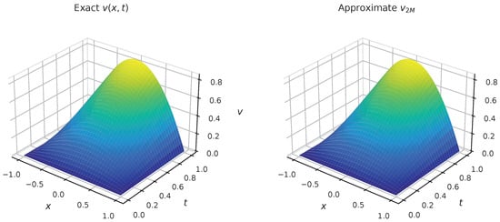
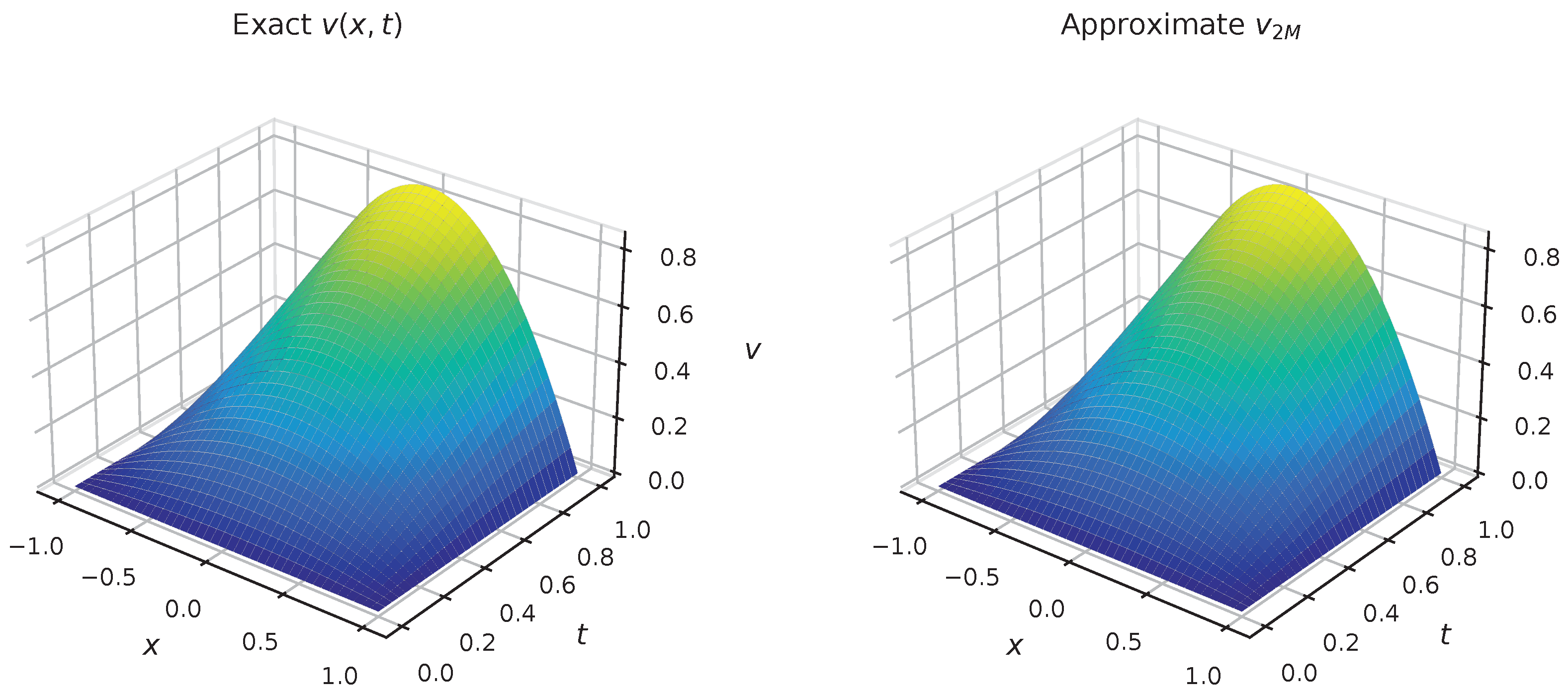
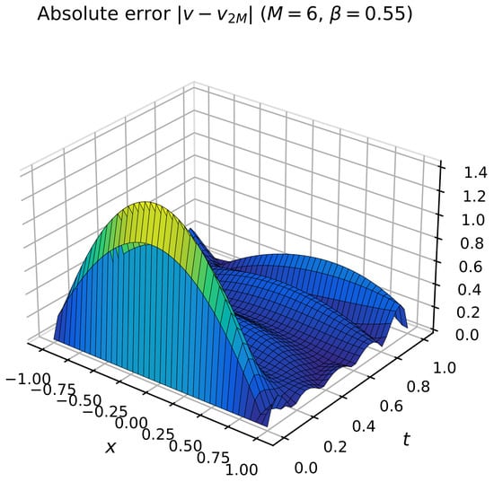
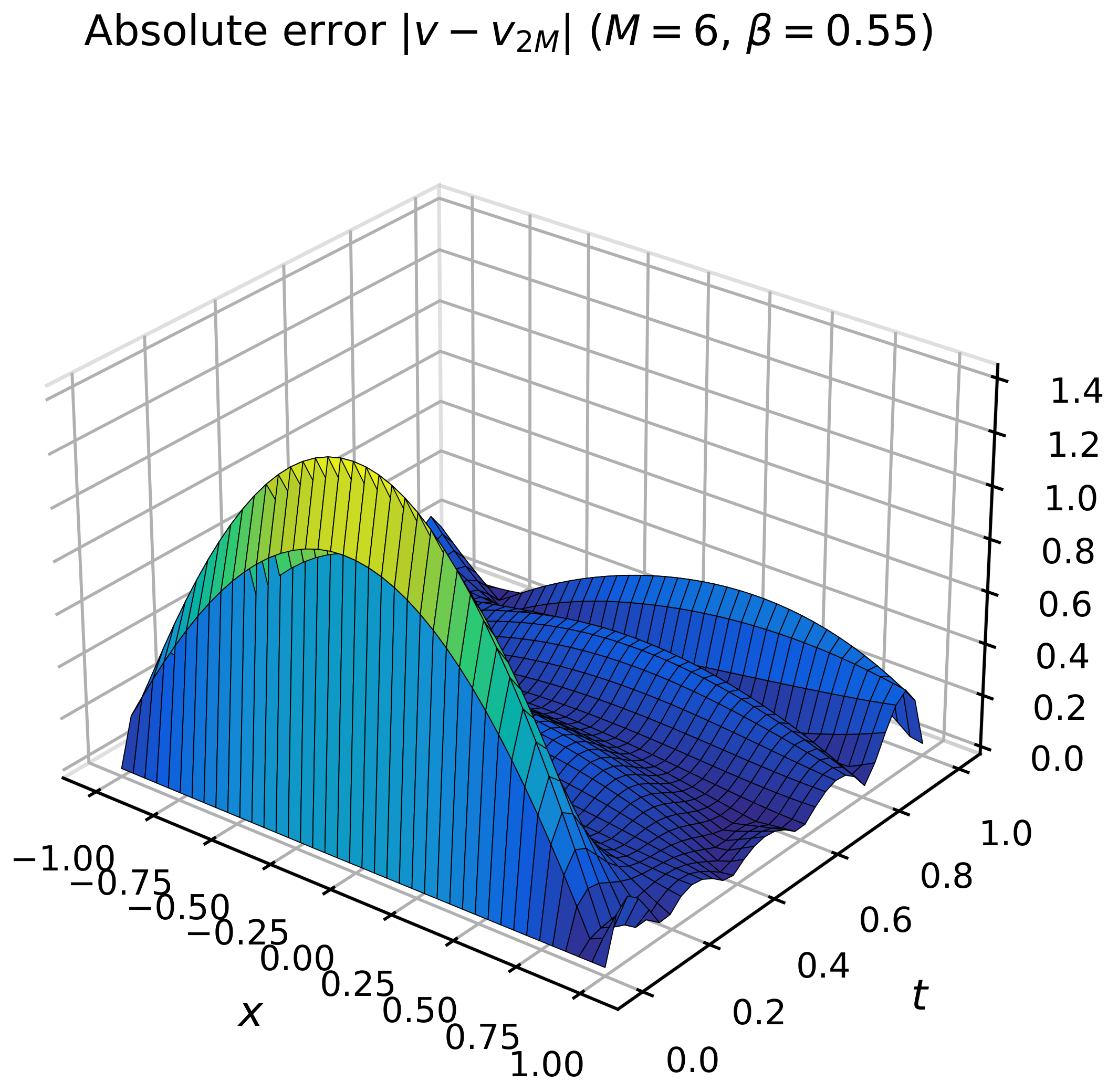
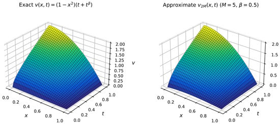
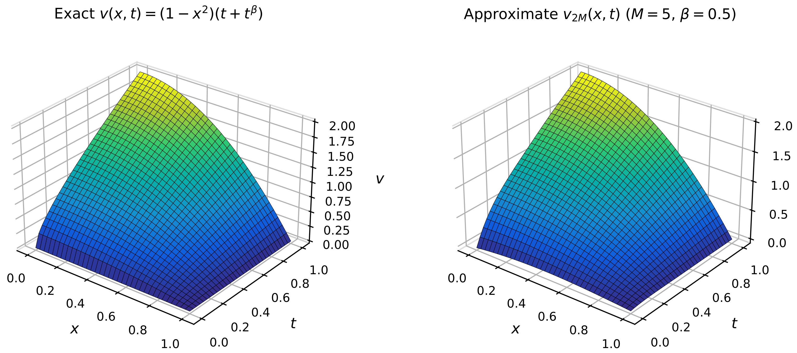
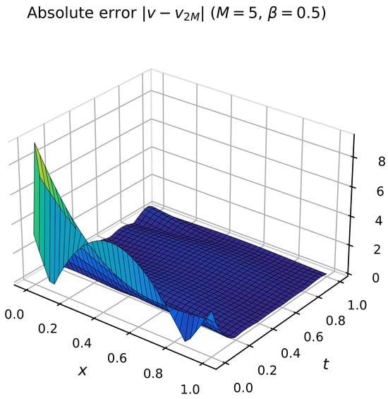
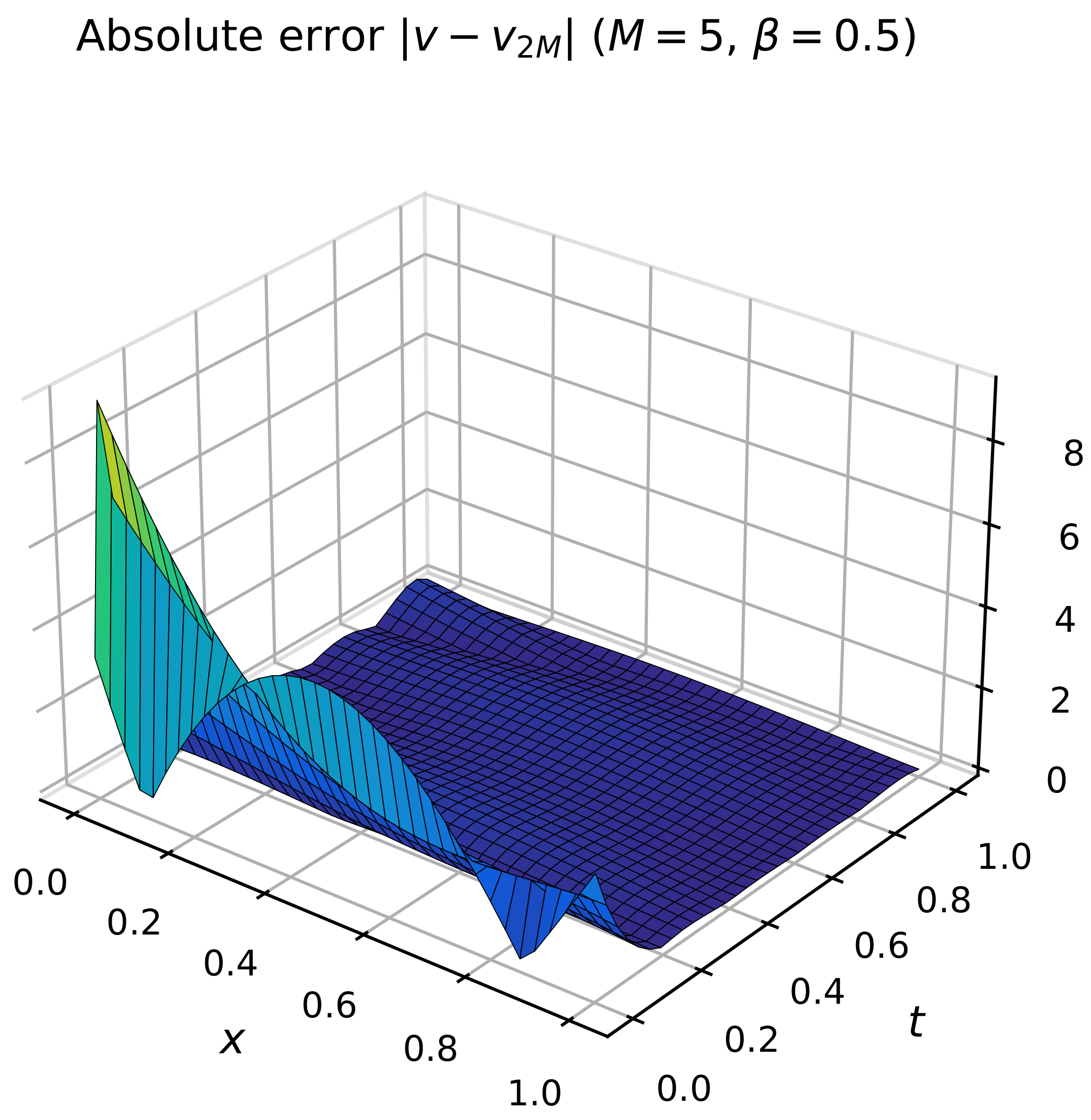
In the numerical experiments below, the overdetermined collocation system is solved in the least-squares sense after column equilibration of the discrete matrix (a standard diagonal scaling that, in exact arithmetic, preserves the least-squares minimizer of ${\parallel Ac-b\parallel }_2$). Table 1 reports the exact solution, the approximate solution, and the absolute error for $M=6$ and $\beta =0.55$ at selected time levels along the diagonal $x=t$. Figure 1 compares the exact and approximate solutions over the computational domain, and Figure 2 shows the corresponding absolute-error field.

Table 1. Numerical results for Example 1 with $M=6$, $\beta =0.55$, and selected time levels along $x=t$.

t	$\mathit{v}\mathbf{(}\mathit{x}\mathbf{,}\mathit{t}\mathbf{)}$	${\mathit{v}}_{\mathbf{2}\mathit{M}}\mathbf{(}\mathit{x}\mathbf{,}\mathit{t}\mathbf{)}$	$\mathbf{|}\mathit{v}\mathbf{(}\mathit{x}\mathbf{,}\mathit{t}\mathbf{)}\mathbf{-}{\mathit{v}}_{\mathbf{2}\mathit{M}}\mathbf{(}\mathit{x}\mathbf{,}\mathit{t}\mathbf{)}\mathbf{|}$
$0.00$	$0.0000$	$1.8239\times {10}^{-11}$	$1.8239\times {10}^{-11}$
$0.10$	$9.8835\times {10}^{-2}$	$9.8835\times {10}^{-2}$	$1.2417\times {10}^{-7}$
$0.20$	$1.9072\times {10}^{-1}$	$1.9072\times {10}^{-1}$	$3.5802\times {10}^{-8}$
$0.30$	$2.6892\times {10}^{-1}$	$2.6892\times {10}^{-1}$	$1.2395\times {10}^{-8}$
$0.40$	$3.2711\times {10}^{-1}$	$3.2711\times {10}^{-1}$	$1.8462\times {10}^{-8}$
$0.50$	$3.5957\times {10}^{-1}$	$3.5957\times {10}^{-1}$	$1.1093\times {10}^{-8}$
$0.60$	$3.6137\times {10}^{-1}$	$3.6137\times {10}^{-1}$	$3.9263\times {10}^{-9}$
$0.70$	$3.2855\times {10}^{-1}$	$3.2855\times {10}^{-1}$	$1.2481\times {10}^{-8}$
$0.80$	$2.5825\times {10}^{-1}$	$2.5825\times {10}^{-1}$	$1.1042\times {10}^{-8}$
$0.90$	$1.4883\times {10}^{-1}$	$1.4883\times {10}^{-1}$	$2.1527\times {10}^{-8}$
$1.00$	$0.0000$	$1.7023\times {10}^{-9}$	$1.7023\times {10}^{-9}$

Figure 1. Exact and approximate solution surfaces for Example 1 with $M=6$ and $\beta =0.55$.

Figure 2. Absolute-error surface $|v-v_{2M}|$ for Example 1 with $M=6$ and $\beta =0.55$.

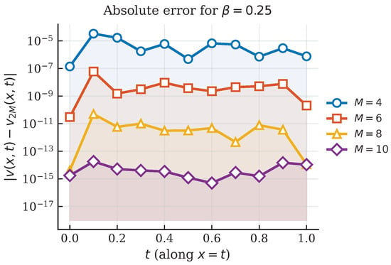
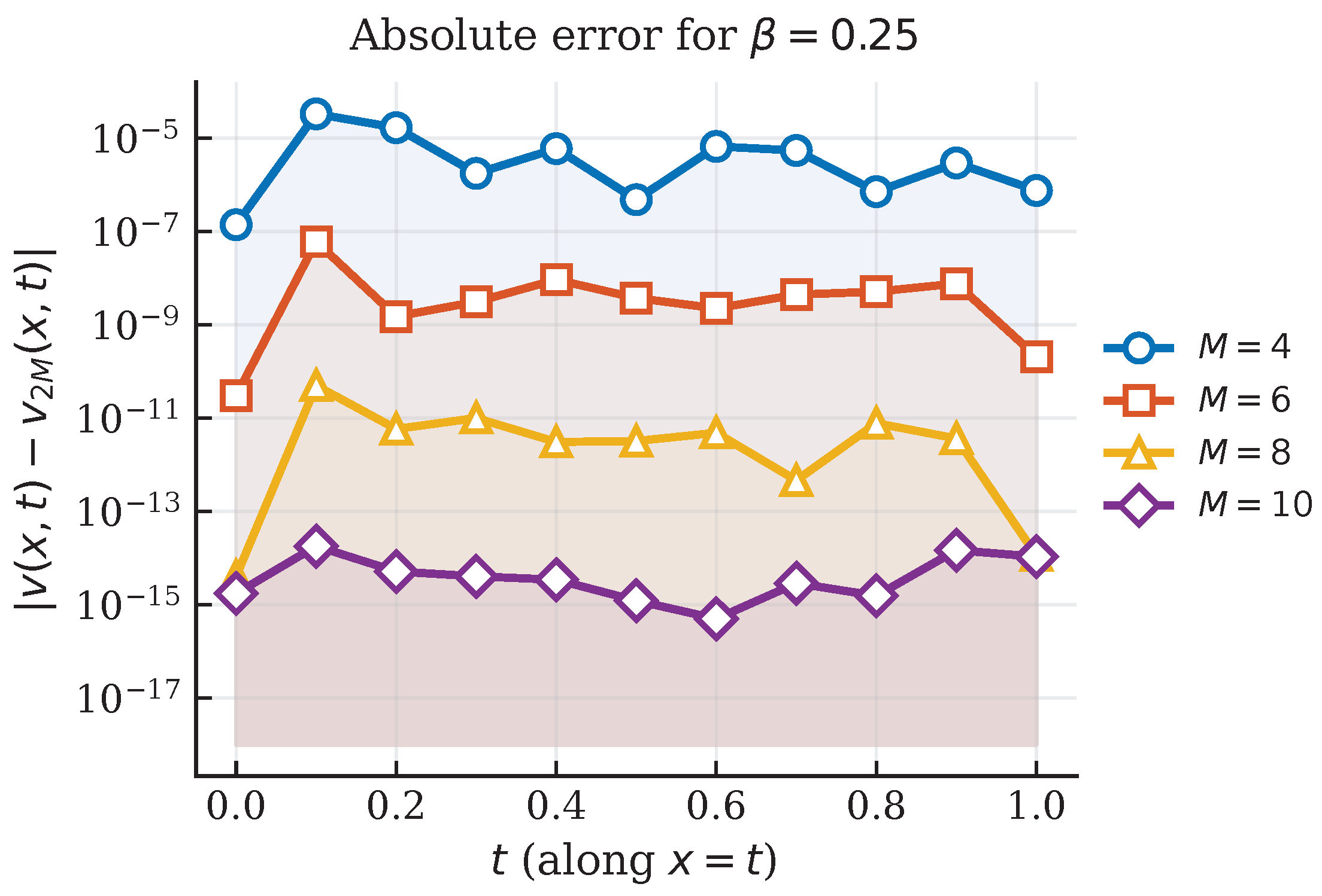
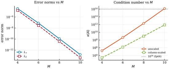
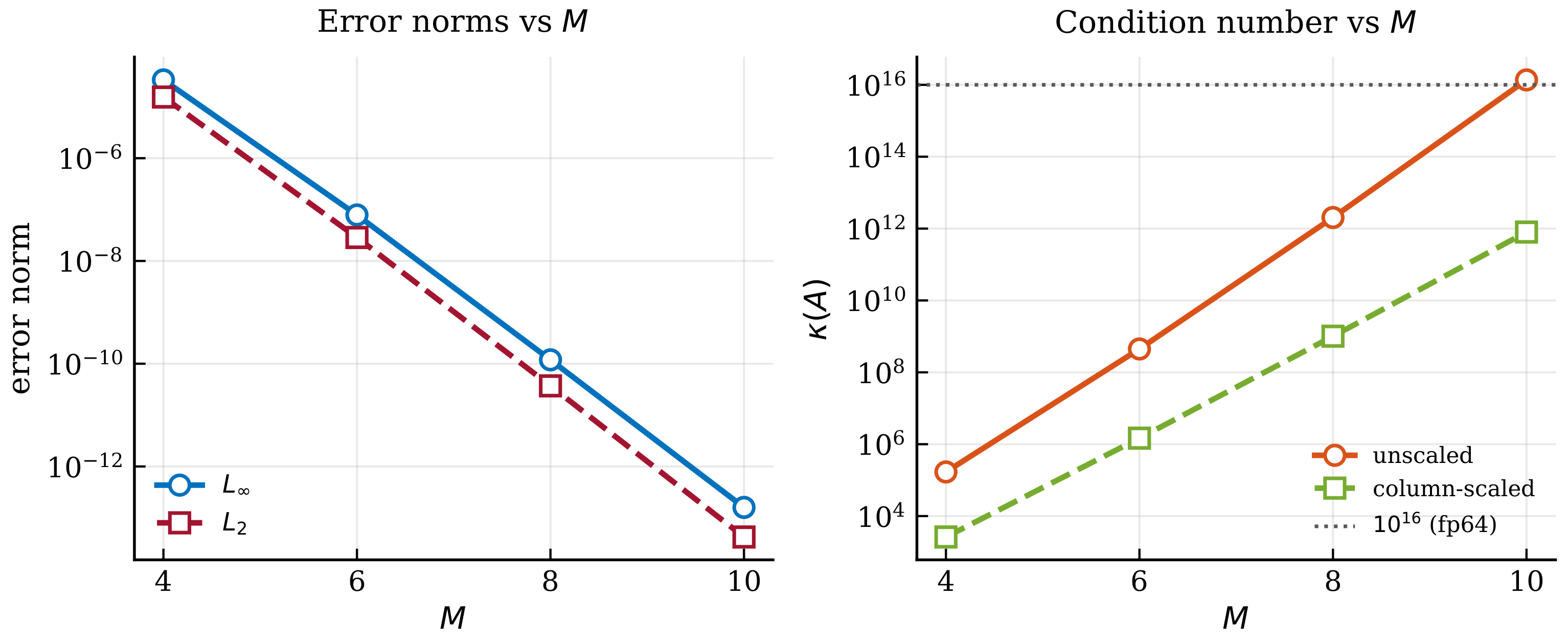
Table 2 presents the absolute errors along $x=t$ for $M=4,6,8,10$ with $\beta =0.25$; the errors decrease systematically as M increases. Figure 3 displays these diagonal errors on a logarithmic scale, and Figure 4 reports the $L_2$ and $L_{\infty }$ norms together with the growth of the (unscaled and column-scaled) condition numbers. Table 3 lists the global error norms, the CPU time, and the observed successive $L_{\infty }$ rates for the same values of M. The large empirical rates indicate rapid error decay for the smooth manufactured solution considered here. Without column equilibration the discrete system at $M=10$ becomes severely ill-conditioned; with the scaling used here the accuracy continues to improve, while Figure 4 makes the residual growth of $\kappa \left(A\right)$ transparent.

Table 2. Absolute errors for Example 1 with $M=4,6,8,10$, $\beta =0.25$, and selected time levels along $x=t$.

t	$\mathit{M}\mathbf{=}\mathbf{4}$	$\mathit{M}\mathbf{=}\mathbf{6}$	$\mathit{M}\mathbf{=}\mathbf{8}$	$\mathit{M}\mathbf{=}\mathbf{10}$
$0.00$	$1.3970\times {10}^{-7}$	$3.0153\times {10}^{-11}$	$4.0779\times {10}^{-15}$	$1.7418\times {10}^{-15}$
$0.10$	$3.3177\times {10}^{-5}$	$6.0593\times {10}^{-8}$	$4.9866\times {10}^{-11}$	$1.8041\times {10}^{-14}$
$0.20$	$1.6798\times {10}^{-5}$	$1.5115\times {10}^{-9}$	$5.8591\times {10}^{-12}$	$5.1625\times {10}^{-15}$
$0.30$	$1.7609\times {10}^{-6}$	$3.1217\times {10}^{-9}$	$1.0024\times {10}^{-11}$	$4.0523\times {10}^{-15}$
$0.40$	$5.9769\times {10}^{-6}$	$9.2619\times {10}^{-9}$	$3.0775\times {10}^{-12}$	$3.4417\times {10}^{-15}$
$0.50$	$4.8102\times {10}^{-7}$	$3.7452\times {10}^{-9}$	$3.2287\times {10}^{-12}$	$1.2212\times {10}^{-15}$
$0.60$	$6.6602\times {10}^{-6}$	$2.2538\times {10}^{-9}$	$4.8442\times {10}^{-12}$	$4.9960\times {10}^{-16}$
$0.70$	$5.4517\times {10}^{-6}$	$4.4350\times {10}^{-9}$	$4.6324\times {10}^{-13}$	$2.8866\times {10}^{-15}$
$0.80$	$7.1436\times {10}^{-7}$	$5.1404\times {10}^{-9}$	$7.7791\times {10}^{-12}$	$1.5543\times {10}^{-15}$
$0.90$	$2.9504\times {10}^{-6}$	$7.6538\times {10}^{-9}$	$3.6566\times {10}^{-12}$	$1.4738\times {10}^{-14}$
$1.00$	$7.5738\times {10}^{-7}$	$2.0767\times {10}^{-10}$	$1.1310\times {10}^{-14}$	$1.0697\times {10}^{-14}$

Figure 3. Absolute error along $x=t$ for Example 1 with $\beta =0.25$ and $M=4,6,8,10$.

Figure 4. Error norms (left) and condition numbers (right) versus M for Example 1 with $\beta =0.25$.

Table 3. $L_2$- and $L_{\infty }$-norms, CPU time, and observed successive rates for Example 1 with $\beta =0.25$. The rate from M to $M^{\prime }$ is $\varrho =\log (E_M/E_{M^{\prime }})/\log (M^{\prime }/M)$ with $E_M={\parallel v-v_{2M}\parallel }_{\infty }$.

M	${\mathit{L}}_{\mathbf{2}}$	${\mathit{L}}_{\mathit{\infty }}$	CPU Time (s)	$\mathit{\varrho }$ (${\mathit{L}}_{\mathit{\infty }}$)
4	$1.5499\times {10}^{-5}$	$3.3436\times {10}^{-5}$	$0.008$	—
6	$2.8635\times {10}^{-8}$	$7.8641\times {10}^{-8}$	$0.029$	$14.93$
8	$3.7078\times {10}^{-11}$	$1.1899\times {10}^{-10}$	$0.078$	$22.57$
10	$4.2386\times {10}^{-14}$	$1.5965\times {10}^{-13}$	$0.181$	$29.64$

Example 2.

We consider Equations (1) and (2) on the domain $[0,1]\times (0,1]$, with

$$\begin{array}{c}h(x,t)=1,\hfill \\ K(x,t,s)=-x(t-s),\hfill \\ f(x,t)=(1-x^2)\left({\displaystyle \frac{t^{1-\beta }}{\Gamma (2-\beta )}}+\Gamma (1+\beta )\right)+2(t+t^{\beta })+x(1-x^2)\left({\displaystyle \frac{t^3}{6}}+{\displaystyle \frac{t^{2+\beta }}{(1+\beta )(2+\beta )}}\right),\hfill \end{array}$$

exact solution $v(x,t)=(1-x^2)(t+t^{\beta })$, and initial and boundary conditions $v(x,0)=0$, $v(0,t)=t+t^{\beta }$, $v(1,t)=0$ [25]. The forcing term is consistent with this data for $h(x,t)=1$ and $K(x,t,s)=-x(t-s)$.

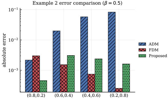
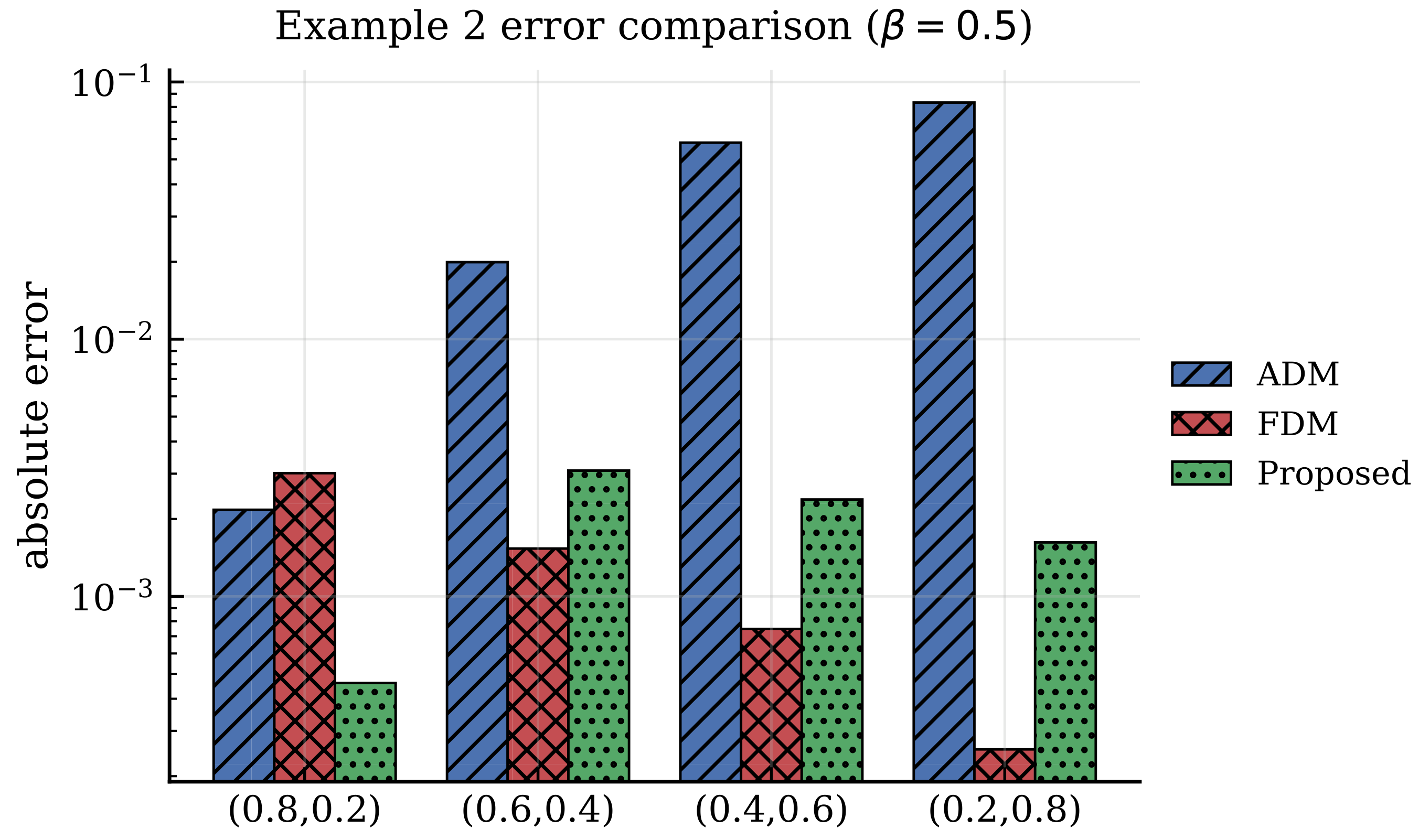
Reference results obtained by the Adomian decomposition method (ADM) with $n=20$ terms and the finite difference method (FDM) with $M=N=10$ are taken from [25]; those reference solvers were not re-implemented here. The proposed Pell–Lucas collocation method is applied with $M=5$ and $\beta =0.5,0.7$, using the same least-squares collocation solve with column equilibration as in Example 1. Table 4 compares solution values at selected sample points, and Table 5 reports the corresponding absolute errors. The comparisons with ADM and FDM are based on pointwise error values reported in the literature; corresponding CPU timings are unavailable or are not directly comparable across implementations and computing environments.

Table 4. Comparison of the proposed method ($M=5$) with ADM ($n=20$) and FDM ($M=N=10$) for selected $(x,t)$ and $\beta =0.5,0.7$ in Example 2. ADM/FDM values are from [25].

$\mathbf{(}\mathit{x}\mathbf{,}\mathit{t}\mathbf{)}$	$\mathit{\beta }\mathbf{=}\mathbf{0.5}$				$\mathit{\beta }=\mathbf{0.7}$
	Exact	ADM	FDM	Proposed	Exact	ADM	FDM	Proposed
$(0.9,0.1)$	$0.0791$	$0.0790$	$0.0748$	$0.0705$	$0.0569$	$0.0569$	$0.0538$	$0.0532$
$(0.7,0.3)$	$0.4323$	$0.4241$	$0.4302$	$0.4358$	$0.3726$	$0.3706$	$0.3701$	$0.3754$
$(0.5,0.5)$	$0.9053$	$0.8680$	$0.9042$	$0.9075$	$0.8367$	$0.8248$	$0.8353$	$0.8392$
$(0.3,0.7)$	$1.3984$	$1.3218$	$1.3979$	$1.4015$	$1.3459$	$1.3166$	$1.3453$	$1.3476$
$(0.1,0.9)$	$1.8302$	$1.7661$	$1.8301$	$1.8266$	$1.8106$	$1.7824$	$1.8105$	$1.8097$

Table 5. Absolute errors of ADM, FDM, and the proposed method ($M=5$) for selected $(x,t)$ and $\beta =0.5,0.7$ in Example 2. ADM/FDM errors are from [25].

$\mathbf{(}\mathit{x}\mathbf{,}\mathit{t}\mathbf{)}$	$\mathit{\beta }\mathbf{=}\mathbf{0.5}$			$\mathit{\beta }\mathbf{=}\mathbf{0.7}$
	ADM	FDM	Proposed	ADM	FDM	Proposed
$(0.8,0.2)$	$2.1713\times {10}^{-3}$	$3.0136\times {10}^{-3}$	$4.6057\times {10}^{-4}$	$4.0422\times {10}^{-4}$	$3.1136\times {10}^{-3}$	$1.8780\times {10}^{-3}$
$(0.6,0.4)$	$1.9929\times {10}^{-2}$	$1.5344\times {10}^{-3}$	$3.0836\times {10}^{-3}$	$5.5585\times {10}^{-3}$	$1.8397\times {10}^{-3}$	$2.8855\times {10}^{-3}$
$(0.4,0.6)$	$5.8106\times {10}^{-2}$	$7.4680\times {10}^{-4}$	$2.3809\times {10}^{-3}$	$2.0409\times {10}^{-2}$	$9.4712\times {10}^{-4}$	$1.9256\times {10}^{-3}$
$(0.2,0.8)$	$8.3181\times {10}^{-2}$	$2.5420\times {10}^{-4}$	$1.6212\times {10}^{-3}$	$4.4305\times {10}^{-2}$	$3.6554\times {10}^{-4}$	$1.1497\times {10}^{-3}$

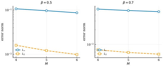
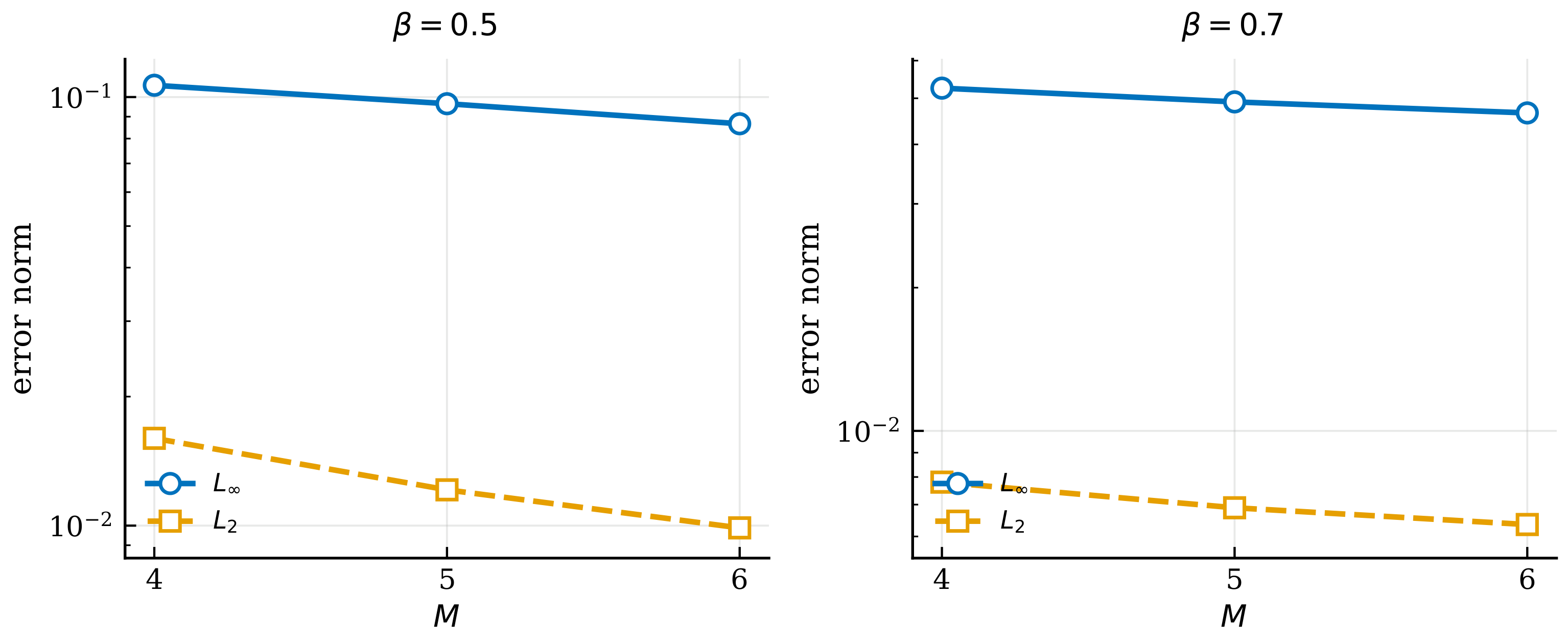
Figure 5 shows the exact and approximate solutions for $\beta =0.5$, Figure 6 the absolute-error field, and Figure 7 a logarithmic comparison of absolute errors at the Table 5 nodes. Because the exact solution contains the weakly singular factor $t^{\beta }$, global polynomial accuracy is limited near $t=0$; nevertheless, Table 6 and Figure 8 show that the $L_2$ and $L_{\infty }$ norms decrease as M increases from 4 to 6, with modest CPU times.

Figure 5. Exact and approximate solution surfaces for Example 2 with $M=5$ and $\beta =0.5$.

Figure 6. Absolute-error surface $|v-v_{2M}|$ for Example 2 with $M=5$ and $\beta =0.5$.

Figure 7. Absolute-error comparison at selected nodes for Example 2 ($\beta =0.5$; ADM/FDM from [25]).

Table 6. $L_2$- and $L_{\infty }$-norms and CPU time for Example 2.

M	$\mathit{\beta }$	${\mathit{L}}_{\mathbf{2}}$	${\mathit{L}}_{\mathit{\infty }}$	CPU Time (s)
4	$0.5$	$1.5985\times {10}^{-2}$	$1.0655\times {10}^{-1}$	$0.007$
5	$0.5$	$1.2120\times {10}^{-2}$	$9.6501\times {10}^{-2}$	$0.016$
6	$0.5$	$9.8802\times {10}^{-3}$	$8.6653\times {10}^{-2}$	$0.026$
4	$0.7$	$7.8039\times {10}^{-3}$	$5.2520\times {10}^{-2}$	$0.007$
5	$0.7$	$6.8937\times {10}^{-3}$	$4.9138\times {10}^{-2}$	$0.014$
6	$0.7$	$6.3568\times {10}^{-3}$	$4.6584\times {10}^{-2}$	$0.025$

Figure 8. Global $L_2$ and $L_{\infty }$ error norms versus M for Example 2.

8. Conclusions

This paper developed a Pell–Lucas collocation method for time-fractional partial integro-differential equations with Caputo fractional derivatives, spatial diffusion, and a Volterra memory term. The unknown solution was approximated by a truncated bivariate Pell–Lucas expansion, and operational matrices were used to represent the fractional-time derivative, spatial derivatives, and integral term. The governing equation together with the initial and boundary conditions was discretized at uniform collocation points, yielding a system of algebraic equations for the expansion coefficients.

An upper error bound in the infinity norm and a residual-based error-estimation procedure were also presented. In Example 1, the approximate solution agreed closely with the exact solution, and the reported error norms decreased systematically for $M=4,6,8,10$ after column equilibration. In Example 2, recomputed collocation values were compared with ADM and FDM results taken from the literature; the method remains competitive at the reported sample points, while global norms improve mildly with M despite the limited regularity induced by $t^{\beta }$. Further study for additional equation classes and comparison settings remains a natural direction for future work.

References

- Appell, J.; Kalitvin, A.; Zabrejko, P. Partial Integral Operators and Integro-Differential Equations: Pure and Applied Mathematics; CRC Press: Boca Raton, FL, USA, 2000. [Google Scholar]
- Grasselli, M.; Kabanikhin, S.; Lorenzi, A. An inverse hyperbolic integrodifferential problem arising in geophysics ii. Nonlinear Anal. Theory Methods Appl. 1990, 15, 283–298. [Google Scholar] [CrossRef] [Scilit]
- Miller, R. An integrodifferential equation for rigid heat conductors with memory. J. Math. Anal. Appl. 1978, 66, 313–332. [Google Scholar] [CrossRef] [Scilit]
- Pao, C. Solution of a nonlinear integrodifferential system arising in nuclear reactor dynamics. J. Math. Anal. Appl. 1974, 48, 470–492. [Google Scholar] [CrossRef] [Scilit]
- Yüzbaşı, Ş.; Yıldırım, G. A collocation method to solve the parabolic-type partial integro-differential equations via pell–lucas polynomials. Appl. Math. Comput. 2022, 421, 126956. [Google Scholar] [CrossRef] [Scilit]
- Yuldashev, T. Nonlocal boundary value problem for a nonlinear fredholm integro-differential equation with degenerate kernel. Differ. Equ. 2018, 54, 1646–1653. [Google Scholar] [CrossRef] [Scilit]
- Dehghan, M.; Shakeri, F. Solution of parabolic integro-differential equations arising in heat conduction in materials with memory via he’s variational iteration technique. Int. J. Numer. Methods Biomed. Eng. 2010, 26, 705–715. [Google Scholar] [CrossRef] [Scilit]
- Fairweather, G. Spline collocation methods for a class of hyperbolic partial integro-differential equations. SIAM J. Numer. Anal. 1994, 31, 444–460. [Google Scholar] [CrossRef] [Scilit]
- Samko, S. Fractional Integrals and Derivatives: Theory and Applications; Gordan and Breach Science: London, UK, 1993. [Google Scholar]
- Mainardi, F. Fractional Calculus: Some Basic Problems in Continuum and Statistical Mechanics; Springer: Berlin/Heidelberg, Germany, 1997. [Google Scholar]
- Kumar, D.; Baleanu, D. Fractional Calculus and Its Applications in Physics; Frontiers Media SA: Lausanne, Switzerland, 2019. [Google Scholar]
- Diethelm, K.; Ford, N. The Analysis of Fractional Differential Equations; Lecture Notes in Mathematics; Springer: Berlin/Heidelberg, Germany, 2010. [Google Scholar]
- Hilfer, R. Applications of Fractional Calculus in Physics; World Scientific: Singapore, 2000. [Google Scholar]
- Podlubny, I. Fractional Differential Equations: An Introduction to Fractional Derivatives, Fractional Differential Equations, to Methods of Their Solution and Some of Their Applications; Elsevier: Amsterdam, The Netherlands, 1998; Volume 198. [Google Scholar]
- Abd Elaziz El-Sayed, A.; Boulaaras, S.; Sweilam, N. Numerical solution of the fractional-order logistic equation via the first-kind dickson polynomials and spectral tau method. Math. Methods Appl. Sci. 2023, 46, 8004–8017. [Google Scholar] [CrossRef] [Scilit]
- Noeiaghdam, S.; Dreglea, A.; Işık, H.; Suleman, M. A comparative study between discrete stochastic arithmetic and floating-point arithmetic to validate the results of fractional order model of malaria infection. Mathematics 2021, 9, 1435. [Google Scholar] [CrossRef] [Scilit]
- Ali, Z.; Nia, S.N.; Rabiei, F.; Shah, K.; Tan, M.K. A semianalytical approach to the solution of time-fractional navier-stokes equation. Adv. Math. Phys. 2021, 2021, 5547804. [Google Scholar] [CrossRef] [Scilit]
- Atangana, A.; Secer, A. A note on fractional order derivatives and table of fractional derivatives of some special functions. Abstr. Appl. Anal. 2013, 2013, 279681. [Google Scholar] [CrossRef] [Scilit]
- Noeiaghdam, S.; Micula, S.; Nieto, J.J. A novel technique to control the accuracy of a nonlinear fractional order model of covid-19: Application of the cestac method and the cadna library. Mathematics 2021, 9, 1321. [Google Scholar] [CrossRef] [Scilit]
- Mainardi, F. Fractional Calculus and Waves in Linear Viscoelasticity: An Introduction to Mathematical Models; World Scientific: Singapore, 2022. [Google Scholar]
- Janmohammadi, A.; Damirchi, J.; Mahmoudi, S.M.; Esfandiari, A. Numerical solutions of inverse time fractional coupled burgers’ equations by the chebyshev wavelet method. J. Appl. Math. Comput. 2022, 68, 2983–3009. [Google Scholar] [CrossRef] [Scilit]
- Foadian, S.; Pourgholi, R.; Tabasi, S.H.; Damirchi, J. The inverse solution of the coupled nonlinear reaction–diffusion equations by the haar wavelets. Int. J. Comput. Math. 2019, 96, 105–125. [Google Scholar] [CrossRef] [Scilit]
- Aslan, E.; Kürkçü, Ö.K.; Sezer, M. A fast numerical method for fractional partial integro-differential equations with spatial-time delays. Appl. Numer. Math. 2021, 161, 525–539. [Google Scholar] [CrossRef] [Scilit]
- Yıldırım, G.; Yüzbaşı, Ş. A collocation technique via Pell-Lucas polynomials to solve fractional differential equation model for HIV/AIDS with treatment compartment. Comput. Model. Eng. Sci. 2024, 141, 281–310. [Google Scholar] [CrossRef] [Scilit]
- Santra, S.; Mohapatra, J. A novel finite difference technique with error estimate for time fractional partial integro-differential equation of volterra type. J. Comput. Appl. Math. 2022, 400, 113746. [Google Scholar] [CrossRef] [Scilit]
- Luo, Z.; Zhang, X.; Wang, S.; Yao, L. Numerical approximation of time fractional partial integro-differential equation based on compact finite difference scheme. Chaos Solitons Fractals 2022, 161, 112395. [Google Scholar] [CrossRef] [Scilit]
- Jaradat, H.; Awawdeh, F.; Rawashdeh, E. Analytic solution of fractional integro-differential equations. Ann. Univ. Craiova-Math. Comput. Sci. Ser. 2011, 38, 1–10. [Google Scholar]
- Hussain, A.K.; Rusli, N.; Fadhel, F.S.; Yahya, Z.R. Solution of one-dimensional fractional order partial integro-differential equations using variational iteration method. AIP Conf. Proc. 2016, 1775, 030096. [Google Scholar] [CrossRef] [Scilit]
- Nawaz, Y. Variational iteration method and homotopy perturbation method for fourth-order fractional integro-differential equations. Comput. Math. Appl. 2011, 61, 2330–2341. [Google Scholar] [CrossRef] [Scilit]
- Dehestani, H.; Ordokhani, Y.; Razzaghi, M. Pseudo-operational matrix method for the solution of variable-order fractional partial integro-differential equations. Eng. Comput. 2021, 37, 1791–1806. [Google Scholar] [CrossRef] [Scilit]
- Abu Arqub, O. Computational algorithm for solving singular fredholm time-fractional partial integrodifferential equations with error estimates. J. Appl. Math. Comput. 2019, 59, 227–243. [Google Scholar] [CrossRef] [Scilit]
- Aslefallah, M.; Shivanian, E. Nonlinear fractional integro-differential reaction-diffusion equation via radial basis functions. Eur. Phys. J. Plus 2015, 130, 47. [Google Scholar] [CrossRef] [Scilit]
- He, J.H.; El-Dib, Y.O. A tutorial introduction to the two-scale fractal calculus and its application to the fractal Zhiber–Shabat oscillator. Fractals 2021, 29, 2150268. [Google Scholar] [CrossRef] [Scilit]
- He, C.H.; He, J.H. Fractal, fractional calculus, and AI: Advanced tools driving innovation in mechanical engineering. Facta Univ. Ser. Mech. Eng. 2026, 24, 1–20. [Google Scholar] [CrossRef] [Scilit]
- He, J.H. A short review on analytical methods for a fully fourth-order nonlinear integral boundary value problem with fractal derivatives. Int. J. Numer. Methods Heat Fluid Flow 2020, 30, 4933–4943. [Google Scholar] [CrossRef] [Scilit]
- Yüzbaşı, Ş.; Yıldırım, G. Pell–Lucas collocation method for numerical solutions of two population models and residual correction. J. Taibah Univ. Sci. 2020, 14, 1262–1278. [Google Scholar] [CrossRef] [Scilit]
- Abd-Elhameed, W.M.; Alshehri, H.M.; Alharbi, M.H.; Alqubori, O.M.; Amin, A.K.; Atta, A.G. Shifted Pell–Lucas polynomial-based algorithms for fractional and classical Rosenau–Hyman models. Fractal Fract. 2026, 10, 359. [Google Scholar] [CrossRef] [Scilit]
- Sweilam, N.H.; Abou Hasan, M.M. Numerical approximation of Lévy–Feller fractional diffusion equation via Chebyshev–Legendre collocation method. Eur. Phys. J. Plus 2016, 131, 251. [Google Scholar] [CrossRef] [Scilit]
- Sweilam, N.H.; Abou Hasan, M.M. An improved method for nonlinear variable-order Lévy–Feller advection–dispersion equation. Bull. Malays. Math. Sci. Soc. 2019, 42, 3021–3046. [Google Scholar] [CrossRef] [Scilit]
- Sweilam, N.H.; Abou Hasan, M.M. Numerical studies for the fractional Schrödinger equation with the quantum Riesz–Feller derivative. Prog. Fract. Differ. Appl. 2016, 2, 231–245. [Google Scholar] [CrossRef] [Scilit]
- Koshy, T.; Koshy, T. Pell and Pell–Lucas Numbers; Springer: Berlin/Heidelberg, Germany, 2014. [Google Scholar]
- El-Sayed, A.A.E. Pell-lucas polynomials for numerical treatment of the nonlinear fractional-order duffing equation. Demonstr. Math. 2023, 56, 20220220. [Google Scholar] [CrossRef] [Scilit]
- Yüzbaşı, Ş.; Yıldırım, G. Pell–Lucas collocation method for solving a class of second order nonlinear differential equations with variable delays. Turk. J. Math. 2023, 47, 37–55. [Google Scholar] [CrossRef] [Scilit]
- Yüzbaşı, Ş.; Yıldırım, G. Pell–Lucas collocation method to solve high-order linear Fredholm–Volterra integro-differential equations and residual correction. Turk. J. Math. 2020, 44, 1065–1091. [Google Scholar] [CrossRef] [Scilit]
- Jafari, H.; Ganji, R.; Salati, S.; Johnston, S. A mixed-method to numerical simulation of variable order stochastic advection diffusion equations. Alex. Eng. J. 2024, 89, 60–70. [Google Scholar] [CrossRef] [Scilit]
- Zhou, T.; Ncube, M.N.; Salati, S.; Jafari, H. Operational matrices for solving a class of variable-order partial differential equations. Fractals 2025, 33, 2540130. [Google Scholar] [CrossRef] [Scilit]
- Şahin, M.; Sezer, M. Pell-lucas collocation method for solving high-order functional differential equations with hybrid delays. Celal Bayar Univ. J. Sci. 2018, 14, 141–149. [Google Scholar] [CrossRef] [Scilit]
- Horadam, A.; Mahon, J. Pell and pell-lucas polynomials. Fibonacci Q. 1985, 23, 7–20. [Google Scholar] [CrossRef] [Scilit]
- Horadam, A.; Swita, B.; Filipponi, P. Integration and derivative sequences for pell and pell-lucas polynomials. Fibonacci Q. 1994, 32, 130–135. [Google Scholar] [CrossRef] [Scilit]
- Abd-Elhameed, W.; Youssri, Y. Generalized lucas polynomial sequence approach for fractional differential equations. Nonlinear Dyn. 2017, 89, 1341–1355. [Google Scholar] [CrossRef] [Scilit]
- Wang, W.; Wang, H. Some results on convolved (p, q)-fibonacci polynomials. Integral Transform. Spec. Funct. 2015, 26, 340–356. [Google Scholar] [CrossRef] [Scilit]
- Meybodi, F.A.A.; Heydari, M.H.; Ghaini, F.M.M. Gaussian-radial basis functions for solving fractional parabolic partial integro-differential equations. J. Math. Ext. 2019, 15, 1–21. [Google Scholar]
- Podlubny, I. Geometric and physical interpretation of fractional integration and fractional differentiation. arXiv 2001, arXiv:math/0110241. [Google Scholar]
Disclaimer/Publisher’s Note: The statements, opinions and data contained in all publications are solely those of the individual author(s) and contributor(s) and not of MDPI and/or the editor(s). MDPI and/or the editor(s) disclaim responsibility for any injury to people or property resulting from any ideas, methods, instructions or products referred to in the content. |
© 2026 by the authors. Licensee MDPI, Basel, Switzerland. This article is an open access article distributed under the terms and conditions of the Creative Commons Attribution (CC BY) license.