Design of Attack-Resilient Load Frequency Control for Hybrid Wind–Diesel Power Systems Under Hybrid Cyber Attacks

Abstract

This paper investigates the finite-time boundedness problem of hybrid wind–diesel power systems through an attack-resilient load frequency control framework in the presence of hybrid cyber attacks and multiple disturbances. The considered disturbances include matched disturbances and mismatched disturbances. To address these challenges, an output-reliant disturbance observer is developed to accurately estimate the matched disturbances, while a dissipative mechanism is employed to attenuate the effects of mismatched disturbances. By utilizing the disturbance estimates and the measured system output, a proportional–integral observer is constructed to estimate the system states. Subsequently, an attack-resilient load frequency controller is designed based on the estimated states and disturbances. Furthermore, multimodal false-data-injection and replay attacks are incorporated into the controller channel to realistically model hybrid cyber threats and enhance controller resilience. Based on Lyapunov stability theory and finite-time stability concepts, sufficient stability conditions are derived in terms of linear matrix inequalities to guarantee finite-time boundedness of the closed-loop system. These conditions also provide a systematic approach for computing the observer and controller gain matrices. Finally, simulation results are presented to demonstrate the effectiveness and robustness of the developed control scheme under hybrid cyber attacks and multiple disturbances.

1. Introduction

Over the last several years, the world has begun shifting its focus toward renewable energy solutions and hybrid wind–diesel power systems (HWDPSs), which are being touted as the pioneers in this regard [1]. Precisely, HWDPSs combine the dependability of diesel generators with the renewable potential of wind turbines in a seamless manner, while resulting in lower fuel use and optimal utilization of the fluctuating wind resources [2]. Additionally, this blending mitigates operational expenses and has a less adverse effect on the environment. Furthermore, these systems improve energy dependability and resilience while simultaneously decreasing dependence on fossil fuels [3]. The development of HWDPSs highlights a transition toward more sustainable and efficient energy infrastructure, driven by advances in control systems, energy storage, and turbine technology [4,5]. In underserved regions around the world, these hybrid systems are transforming power generation by providing reliable energy while simultaneously reducing environmental impact. As wind power is integrated into the system, it is essential to keep the frequency within the specified range to achieve active power balance in a region. Therefore, frequency control of power systems equipped with wind turbine generators has been the subject of study, and some results can be found in [6,7,8,9]. Therefore, load frequency control in HWDPSs has emerged as a critical research problem.

In practice, control systems are susceptible to external disturbances, which could hinder the system’s operation. In light of the foregoing, researchers have devised an assortment of approaches for the rejection and attenuation of disturbances [10,11,12]. Among them, the disturbance observer (DO) has emerged as a powerful framework for compensating external disturbances and uncertainties due to its accuracy, effectiveness, and robustness [10]. In addition, dissipative theory is extensively used in the synthesis and analysis of several sectors of engineering and science to reduce disturbances [12]. However, it should be noted that many real-world systems may be affected by different kinds of disturbances, and each may have different characteristics and consequently require different modeling and compensation strategies [13]. The approaches mentioned earlier are ineffective in this situation because they are designed to handle specific types of disruption. To address this shortcoming, composite anti-disturbance schemes have become prevalent, integrating disturbance-rejection and disturbance-attenuation approaches. In this regard, some notable results have been published for various control systems [14,15,16,17]. It should be emphasized that the matched/mismatched disturbance classification is not restricted to sliding-mode control. It is a structural classification determined by whether a disturbance enters through the control-input subspace. Unlike sliding-mode control, which handles matched disturbances through sliding-surface invariance, the present theoretical framework actively estimates and compensates for the matched disturbance using an output-reliant disturbance observer. Meanwhile, the mismatched disturbance, which cannot generally be cancelled through the control input, is attenuated through the strictly dissipative mechanism. It should be noted that the DOs in the aforementioned results are contingent upon the availability of complete state information. In practice, measurement instruments are able to access only a small portion of system states, which encourages the study of output-reliant DOs [18,19] and observer techniques [20,21]. Furthermore, wind variability, load fluctuations, and environmental uncertainties expose HWDPSs to multiple disturbances. Hence, designing an output-based anti-disturbance control strategy for HWDPSs is of significant practical importance.

Over time, network connections are replacing more traditional point-to-point connections. Although networked communications provide substantial advantages, they pose inherent safety risks. Security is a major issue since dynamical systems allow for more integration between physical and networked areas than ever before, which opens the door for attackers to potentially compromise the system’s stability [22]. As a result, a dynamical system’s security measures have become a vital research area in control engineering [23]. Specifically, adversaries execute two fundamental categories of cyber attacks, namely false-data-injection attacks [24] and replay attacks [25]. To be more precise, false-data-injection attacks are designed to intercept states from communication networks and introduce malicious data into transmitted signals. Furthermore, in a replay attack, hackers continuously transmit data that has been previously recorded. On the other hand, substantial progress has been reported in resilient control under hybrid cyber attacks, particularly under combined denial-of-service and false-data-injection attacks (see [26,27,28,29,30,31,32]), whereas comparatively fewer studies have addressed false-data-injection and replay attacks within a common framework (see [33,34,35,36,37]). Furthermore, multimodal false-data-injection attacks, in which different attack functions represent distinct false-data-injection patterns, have received increasing research attention [38,39]. Motivated by these developments, the present study investigates multimodal false-data-injection and replay attacks within a unified stochastic framework for hybrid wind–diesel power systems, which rely on networked communication channels for transmitting measurement and control information.

It should be noted that exponential and asymptotic stability concepts characterize the long-term behavior of HWDPSs. In contrast, finite-time convergence requires the system states to reach the equilibrium within a finite settling time, which generally depends on the initial conditions [40]. Fixed-time convergence ensures an upper bound on the settling time independent of the initial conditions [41], whereas predefined-time convergence allows the convergence-time bound to be prescribed in advance through suitable design parameters [42]. Unlike these convergence-oriented concepts, finite-time boundedness (FTB) has also been extensively investigated for a variety of dynamic systems [43,44,45]. Rather than requiring the system states to reach the equilibrium within a finite settling time, FTB requires that the system trajectories remain within a prescribed bound over a selected finite interval, subject to admissible initial conditions and disturbances. Accordingly, the objective of the present study is to establish FTB for the considered HWDPS. This objective is particularly relevant to maintaining bounded frequency deviations during critical transient intervals in the presence of hybrid cyber attacks and external disturbances, thereby enhancing the operational resilience of the power system.

Based on the above insights and literature survey, the objective of this study is to develop a DO and an attack-resilient load frequency control (ARLFC) to achieve FTB for HWDPSs with hybrid cyber attacks and multiple external disturbances. More specifically, the main innovations and outcomes of this study are put forth in four aspects:

▪

An ARLFC framework is developed for HWDPSs operating under hybrid cyber attacks and multiple external disturbances. The disturbances are classified into matched disturbances and mismatched disturbances, enabling a realistic representation of adverse operating conditions in HWDPSs.

▪

For the considered HWDPSs, an output-reliant DO is designed to estimate matched disturbances acting on the control input channel. Specifically, the DO relies solely on the measured system output, making it suitable for practical load frequency control applications where full state measurements may not be available.

▪

By utilizing the measured output together with the estimated matched disturbances, a proportional–integral observer (PIO) is constructed to estimate the system states of the HWDPSs. This PIO provides reliable state information for controller synthesis without directly estimating disturbances.

▪

Specifically, the controller explicitly incorporates cyber attacks in the controller channel and mitigates stochastic signal manipulation over compromised communication links. A unified stochastic framework is adopted to represent multimodal false-data-injection and replay attacks, capturing practical behaviors such as multimodal and delayed signal injection, thereby enhancing the relevance of the developed ARLFC for HWDPSs.

Moreover, sufficient conditions guaranteeing FTB for the closed-loop HWDPSs are derived using Lyapunov stability theory and formulated in terms of linear matrix inequalities. Lastly, the simulation results, including Monte Carlo analyses, act as evidence to assess the theoretical findings that have been developed. The DO is shown to effectively reject external disturbances and the HWDPSs are stabilized using the developed controller.

Notations: ${\mathbb{R}}^x$ and ${\mathbb{R}}^{x\times y}$ represent the x-dimensional Euclidean space and the set of all $x\times y$ real matrices, respectively. ${\mathbb{R}}_{+}^x$ denotes the set of all $x\times x$ positive definite matrices, and I is the identity matrix of appropriate dimension. The superscripts T and $-1$ indicate matrix transpose and inverse, respectively. $Pr\{·\}$ and $\mathbb{E}\{·\}$ denote the probability measure and mathematical expectation, respectively. The symbol * refers to symmetric terms in a matrix. For any square matrix $\mathsf{N}$, $sym\left\{\mathsf{N}\right\}=\mathsf{N}+{\mathsf{N}}^T$; ${\mathbb{C}}^{\diamond }$ indicates the pseudoinverse of $\mathbb{C}$ with (i) $\mathbb{C}{\mathbb{C}}^{\diamond }\mathbb{C}=\mathbb{C}$, (ii) ${\mathbb{C}}^{\diamond }\mathbb{C}{\mathbb{C}}^{\diamond }={\mathbb{C}}^{\diamond }$, (iii) ${\left(\mathbb{C}{\mathbb{C}}^{\diamond }\right)}^T=\mathbb{C}{\mathbb{C}}^{\diamond }$ and (iv) ${\left({\mathbb{C}}^{\diamond }\mathbb{C}\right)}^T={\mathbb{C}}^{\diamond }\mathbb{C}$.

2. Model Description and Preliminaries

Generally, linear equations adequately describe the dynamics of load frequency control systems. In this regard, the linearized HWDPS model featuring battery energy storage is taken into account [7,8,9]. The model includes a wind turbine with a pitch angle controller, a diesel generator with a speed regulator, and a battery for energy storage. In this case, the frequency control issue can be adequately studied using a first-order dynamical model of energy storage in batteries and a generator based on wind turbines. In light of the above discussions, as in [7,8,9], its corresponding state-space model is provided hereunder:

$$\begin{array}{c}\hfill \left\{\begin{array}{cc}\dot{\eta }\left(t\right)=\hfill & \mathcal{A}\eta \left(t\right)+\mathcal{B}u\left(t\right)+\mathcal{D}\mu \left(t\right),\hfill \\ \alpha \left(t\right)=\hfill & \mathcal{C}\eta \left(t\right),\hfill \\ {\alpha }_z\left(t\right)=\hfill & {\mathcal{C}}_z\eta \left(t\right),\hfill \end{array}\right.\end{array}$$

(1)

where $\eta \left(t\right)={[{\eta }_1\left(t\right),{\eta }_2\left(t\right),{\eta }_3\left(t\right),{\eta }_4\left(t\right),{\eta }_5\left(t\right),{\eta }_6\left(t\right),{\eta }_7\left(t\right),{\eta }_8\left(t\right),{\eta }_9\left(t\right),{\eta }_{10}\left(t\right),{\eta }_{11}\left(t\right)]}^T\in {\mathbb{R}}^{\eta }$ delineates the state vector of the system; $u\left(t\right)\in {\mathbb{R}}^u$ symbolizes the control input; $\mu \left(t\right)\in {\mathbb{R}}^{\mu }$ denotes the mismatched disturbance; $\alpha \left(t\right)\in {\mathbb{R}}^{\alpha }$ represents the measurement output vector; and ${\alpha }_z\left(t\right)\in {\mathbb{R}}^{{\alpha }_z}$ represents the control output vector. Herein, ${\eta }_1\left(t\right)$↣ incremental change in frequency; ${\eta }_2\left(t\right)$↣ incremental change in diesel generator active power; ${\eta }_3\left(t\right)$↣ incremental change in speed governor valve position; ${\eta }_5\left(t\right)$↣ incremental change in wind generator frequency; ${\eta }_6\left(t\right)$↣ incremental change in wind active power; ${\eta }_7\left(t\right)$↣ incremental change in hydraulic pitch actuator output; and ${\eta }_9\left(t\right)$↣ incremental change in battery active power. Moreover, as in [7,8], ${\eta }_4\left(t\right)$ and ${\eta }_8\left(t\right)$ have been regarded as dummy states for the development of the model; ${\eta }_{10}\left(t\right)$ and ${\eta }_{11}\left(t\right)$ delineate the augmented states leveraged for stability; $\mathcal{C}$ and ${\mathcal{C}}_z$ denote matrices of appropriate dimensions; and $\mathcal{A}$, $\mathcal{B}$ and $\mathcal{D}$ depict the constant matrices of the form:

$$\begin{array}{c}\hfill \mathcal{A}=\left[\begin{array}{cccc}{a}_{11}& a_{12}& \dots & a_{1,11}\\ a_{21}& a_{22}& \dots & a_{2,11}\\ ⋮& ⋮& \ddots & ⋮\\ a_{11,1}& a_{11,2}& \dots & a_{11,11}\end{array}\right],\mathcal{B}=\left[\begin{array}{cc}{b}_{11}& b_{12}\\ b_{21}& b_{22}\\ ⋮& ⋮\\ b_{11,1}& b_{11,2}\end{array}\right]\mathrm{and}\mathcal{D}=\left[\begin{array}{cc}{d}_{11}& d_{12}\\ d_{21}& d_{22}\\ ⋮& ⋮\\ d_{11,1}& d_{11,2}\end{array}\right],\end{array}$$

where

$$\begin{array}{cc}\hfill & \left\{\begin{array}{cc}{a}_{11}\hfill & =-{\displaystyle \frac{1+K_{PT}{K}_{IG}}{T_{PT}}},a_{12}={\displaystyle \frac{K_{PT}}{T_{PT}}},a_{15}={\displaystyle \frac{K_{PT}{K}_{IG}}{T_{PT}}},a_{19}=-{\displaystyle \frac{K_{PT}}{T_{PT}}},\hfill \\ a_{22}\hfill & =-{\displaystyle \frac{1}{T_{D4}}},a_{23}={\displaystyle \frac{1}{T_{D4}}},\hfill \\ a_{31}\hfill & =-{\displaystyle \frac{K_{D1}{T}_{D1}}{R_D{T}_{D2}{T}_{D3}}},a_{33}=-{\displaystyle \frac{1}{T_{D3}}},a_{34}=-{\displaystyle \frac{K_{D1}(T_{D1}-T_{D2})}{T_{D2}{T}_{D3}}},\hfill \\ a_{41}\hfill & =-{\displaystyle \frac{1}{R_D{T}_{D2}}},a_{44}=-{\displaystyle \frac{1}{T_{D2}}},\hfill \\ a_{51}\hfill & ={\displaystyle \frac{K_{IG}}{T_W}},a_{55}={\displaystyle \frac{K_{TP}-K_{IG}-1}{T_W}},a_{56}={\displaystyle \frac{1}{T_W}},\hfill \\ a_{66}\hfill & =-{\displaystyle \frac{1}{T_{P3}}},a_{67}={\displaystyle \frac{K_{PC}{K}_{P3}}{T_{P3}}},\hfill \\ a_{77}\hfill & =-{\displaystyle \frac{1}{T_{P2}}},a_{78}={\displaystyle \frac{K_{P1}{K}_{P2}(1-T_{P1})}{T_{P2}}},\hfill \\ a_{88}\hfill & =-1,\hfill \\ a_{91}\hfill & ={\displaystyle \frac{1}{T_{BES}}},a_{99}=-{\displaystyle \frac{1}{T_{BES}}}.\hfill \end{array}\right.\hfill \\ \hfill & \left\{\begin{array}{cc}{b}_{31}\hfill & ={\displaystyle \frac{K_{D1}{T}_{D1}}{T_{D2}{T}_{D3}}},\hfill \\ b_{41}\hfill & ={\displaystyle \frac{1}{T_{D2}}},\hfill \\ b_{72}\hfill & ={\displaystyle \frac{K_{P1}{K}_{P2}{T}_{P1}}{T_{P2}}},\hfill \\ b_{82}\hfill & =1.\hfill \end{array}\right.\hfill \\ \hfill & \left\{\begin{array}{cc}{d}_{11}\hfill & =-{\displaystyle \frac{K_{PT}}{T_{PT}}},\hfill \\ d_{52}\hfill & ={\displaystyle \frac{1}{T_W}}.\hfill \end{array}\right.\hfill \end{array}$$

The remaining terms in $\mathcal{A}$, $\mathcal{B}$, $\mathcal{D}$ are zero and the description of the symbols used in the system matrices is given in Table 1.

Table 1. Model Parameters [9].

Parameter	Description	Parameter	Description
$K_{PT}$	Power-to-frequency gain of the diesel generator (Hz/pu kW)	$T_{PT}$	Power system time constant (s)
$K_{IG}$	Integral gain related to governor dynamics (pu kW/Hz)	$K_{TP}$	Frequency-to-power gain of the wind turbine (pu kW/Hz)
$T_W$	Wind turbine generator time constant (s)	$K_{PC}$	Pitch controller gain constant
$K_{P1}$	Pitch control subsystem gain (stage 1)	$K_{P2}$	Pitch control subsystem gain (stage 2)
$K_{P3}$	Hydraulic pitch actuator gain constant	$T_{P1}$	Pitch controller time constant (s)
$T_{P2}$	Pitch actuator time constant (s)	$T_{P3}$	Hydraulic pitch actuator time constant (s)
$K_{D1}$	Diesel generator gain constant (pu kW/Hz)	$T_{D1}$	Diesel governor time constant (s)
$T_{D2}$	Diesel actuator time constant (s)	$T_{D3}$	Diesel engine time constant (s)
$T_{D4}$	Diesel generator time constant (s)	$R_D$	Speed droop characteristic (Hz/pu kW)
$T_{BES}$	Battery energy storage system time constant (s)

2.1. Problem Statement

Aside from the mismatched disturbances $\mu \left(t\right)$, it should be noted that the HWDPSs may also be susceptible to matched disturbances. This is owing to the fact that there are control system interactions, interference in communication links, and so on. In this regard, the matched disturbance, denoted by ${\gamma }_1\left(t\right)\in {\mathbb{R}}^u$, is assumed to enter through the control-input path of the system (1). Further, in order to reflect the reality more precisely, the matched disturbance is assumed to be generated by the following exogenous system:

$$\begin{array}{c}\hfill \left\{\begin{array}{cc}\dot{\omega }\left(t\right)=\hfill & \mathcal{T}\omega \left(t\right)+\mathcal{U}{\gamma }_2\left(t\right),\hfill \\ {\gamma }_1\left(t\right)=\hfill & \mathcal{V}\omega \left(t\right),\hfill \end{array}\right.\end{array}$$

(2)

where $\omega \left(t\right)\in {\mathbb{R}}^{\omega }$ denotes the state vector of the exogenous system; ${\gamma }_2\left(t\right)\in {\mathbb{R}}^{\gamma }$ stands for the additional disturbance; and $\mathcal{T}$, $\mathcal{U}$ and $\mathcal{V}$ denote known constant matrices of appropriate dimensions. Based on the above discussions, the system (1) with matched disturbances can be laid out in the following manner:

$$\begin{array}{c}\hfill \left\{\begin{array}{cc}\dot{\eta }\left(t\right)=\hfill & \mathcal{A}\eta \left(t\right)+\mathcal{B}(u\left(t\right)+{\gamma }_1\left(t\right))+\mathcal{D}\mu \left(t\right),\hfill \\ \alpha \left(t\right)=\hfill & \mathcal{C}\eta \left(t\right),\hfill \\ {\alpha }_z\left(t\right)=\hfill & {\mathcal{C}}_z\eta \left(t\right).\hfill \end{array}\right.\end{array}$$

(3)

Here, ${\gamma }_1\left(t\right)$ enters through the control-input channel $\mathcal{B}$ and represents matched input-side perturbations. Meanwhile, ${\mu }_1\left(t\right)$ and ${\mu }_2\left(t\right)$ enter through $\mathcal{D}$ and represent load-demand fluctuations and wind-power intermittency, respectively. The matched disturbance is estimated and compensated, whereas the mismatched disturbances are attenuated using the dissipative mechanism. The admissible disturbances satisfy the finite-horizon energy bound in Assumption 2.

2.2. Layout of Observer Framework

2.2.1. Description of Output-Reliant DO

As detailed in the introduction, one of the significant and practical methods of estimating the disturbances is the DO technique. Prior to constructing the DO, we perform the differential operation on $\alpha \left(t\right)$, and the resulting equation is provided as follows:

$$\begin{array}{cc}\hfill \dot{\alpha }\left(t\right)=& \mathcal{C}\mathcal{A}{\mathcal{C}}^{\diamond }\alpha \left(t\right)+\mathcal{C}\mathcal{B}u\left(t\right)+\mathcal{C}\mathcal{B}{\gamma }_1\left(t\right)+\mathcal{C}\mathcal{D}\mu \left(t\right).\hfill \end{array}$$

(4)

In this regard, as in [18,19], the following DO is designed using the information obtained from (2) and (3):

$$\begin{array}{c}\hfill \left\{\begin{array}{cc}\widehat{\omega }\left(t\right)=\hfill & \sigma \left(t\right)-\mathcal{M}\alpha \left(t\right),\hfill \\ \dot{\sigma }\left(t\right)=\hfill & [\mathcal{T}+\mathcal{M}\mathcal{C}\mathcal{B}\mathcal{V}]\widehat{\omega }\left(t\right)+\mathcal{M}[\mathcal{C}\mathcal{A}{\mathcal{C}}^{\diamond }\alpha \left(t\right)+\mathcal{C}\mathcal{B}u\left(t\right)],\hfill \\ \widehat{{\gamma }_1}\left(t\right)=\hfill & \mathcal{V}\widehat{\omega }\left(t\right),\hfill \end{array}\right.\end{array}$$

(5)

where $\widehat{\omega }\left(t\right)$ and ${\widehat{\gamma }}_1\left(t\right)$ stand for the estimates of $\omega \left(t\right)$ and ${\gamma }_1\left(t\right)$, respectively; $\sigma \left(t\right)$ symbolizes the internal state of the observer; and $\mathcal{M}\in {\mathbb{R}}^{\omega \times \alpha }$ denotes the DO gain matrix, which will be calculated in the subsequent sections.

2.2.2. Description of PIO

Subsequently, to estimate the states of the considered system, the following PIO is constructed by utilizing the output information from the system model (3) and (5):

$$\begin{array}{c}\hfill \left\{\begin{array}{cc}\dot{\widehat{\eta }}\left(t\right)=\hfill & \mathcal{A}\widehat{\eta }\left(t\right)+\mathcal{B}(u\left(t\right)+{\widehat{\gamma }}_1\left(t\right))+{\mathcal{E}}_1(\alpha \left(t\right)-\widehat{\alpha }\left(t\right))+\mathcal{B}\iota \left(t\right),\hfill \\ \widehat{\alpha }\left(t\right)=\hfill & \mathcal{C}\widehat{\eta }\left(t\right),\hfill \\ \dot{\iota }\left(t\right)=\hfill & -\iota \left(t\right)+{\mathcal{E}}_2(\alpha \left(t\right)-\widehat{\alpha }\left(t\right)),\hfill \end{array}\right.\end{array}$$

(6)

where $\widehat{\eta }\left(t\right)$ denotes the estimate of $\eta \left(t\right)$; $\iota \left(t\right)$ denotes the integral state vector; and ${\mathcal{E}}_1\in {\mathbb{R}}^{\eta \times \alpha }$ and ${\mathcal{E}}_2\in {\mathbb{R}}^{u\times \alpha }$ stand for the proportional and integral gain matrices, respectively, and their design will be presented in the subsequent section.

Remark 1.

Unlike conventional observers requiring complete state information, the developed framework combines an output-reliant DO with a PIO. The DO reconstructs the matched disturbance from the measured output, while the integral correction in the PIO improves state-estimation accuracy under persistent disturbances.

2.3. Attack-Resilient Load Frequency Control Scheme

This section focuses on designing a controller to stabilize the system under consideration. Two principal types of attacks are considered: false-data-injection and replay attacks. A unified stochastic framework is used to model these hybrid cyber attacks.

In particular, cyber attacks often intercept and modify the signals transmitted to the controller. On the basis of this, a more realistic multimodal false-data-injection attack model [21] is taken into consideration, and the signal that is transmitted to the controller is laid out in the following manner:

$${\widehat{\eta }}^d\left(t\right)=(1-\nu \left(t\right))\widehat{\eta }\left(t\right)+\nu \left(t\right){\displaystyle \sum _{g=1}^m}{\varphi }_g\left(t\right)l_g\left(\widehat{\eta }\left(t\right)\right),$$

(7)

where $\nu \left(t\right)$ and ${\varphi }_g\left(t\right)$$(g=1,2,\dots ,m)$ stand for the Bernoulli-distributed variables that indicate the occurrence of an attack and the attack mode, respectively; and $l_g\left(\widehat{\eta }\left(t\right)\right)$ represents the nonlinear attack function, which adheres to Assumption 1. Moreover, $\nu \left(t\right)$ and ${\varphi }_g\left(t\right)$ satisfy the following conditions:

$$\begin{array}{c}\hfill \left\{\begin{array}{c}Pr\{\nu \left(t\right)=1\}=\mathbb{E}\left\{\nu \left(t\right)\right\}=\overline{\nu },Pr\{\nu \left(t\right)=0\}=1-\mathbb{E}\left\{\nu \left(t\right)\right\}=1-\overline{\nu },\hfill \\ Pr\{{\varphi }_g\left(t\right)=1\}=\mathbb{E}\left\{{\varphi }_g\left(t\right)\right\}={\overline{\varphi }}_g,Pr\{{\varphi }_g\left(t\right)=0\}=1-\mathbb{E}\left\{{\varphi }_g\left(t\right)\right\}=1-{\overline{\varphi }}_g,\hfill \\ {\displaystyle \sum _{g=1}^m}{\varphi }_g\left(t\right)={\displaystyle \sum _{g=1}^m}{\overline{\varphi }}_g=1,0\le \overline{\nu },{\overline{\varphi }}_g\le 1.\hfill \end{array}\right.\end{array}$$

Moreover, to ease the analysis, let us consider $\beta \left(\widehat{\eta }\left(t\right)\right)={\left[\begin{array}{cccc}{l}_1^T\left(\widehat{\eta }\left(t\right)\right)& l_2^T\left(\widehat{\eta }\left(t\right)\right)& \dots & l_m^T\left(\widehat{\eta }\left(t\right)\right)\end{array}\right]}^T$ and $◊\left(t\right)=\left[\begin{array}{cccc}{\varphi }_1\left(t\right)& {\varphi }_2\left(t\right)& \dots & {\varphi }_m\left(t\right)\end{array}\right]$ with $\overline{◊}=\mathbb{E}\{◊\left(t\right)\}=\left[\begin{array}{ccc}{\overline{\varphi }}_1& \dots & {\overline{\varphi }}_m\end{array}\right]$. Based on this premise, the description in (7) can be equivalently rewritten as follows:

$${\widehat{\eta }}^d\left(t\right)=(1-\nu \left(t\right))\widehat{\eta }\left(t\right)+\nu \left(t\right)◊\left(t\right)\beta \left(\widehat{\eta }\left(t\right)\right).$$

(8)

Remark 2.

The considered hybrid attack model [21] encompasses both general and multimodal false-data-injection scenarios within a unified stochastic framework. In the general case ($m=1$), the false-data-injection attack reduces to a single attack function, and the corrupted signal becomes ${\widehat{\eta }}^d\left(t\right)=(1-\nu \left(t\right))\widehat{\eta }\left(t\right)+\nu \left(t\right)l_1\left(\widehat{\eta }\left(t\right)\right)$, which represents a conventional false-data-injection attack model. In the multimodal case ($m>1$), multiple nonlinear attack functions coexist with ${\displaystyle \sum _{g=1}^m}{\varphi }_g\left(t\right)=1$. Consequently, the injected signal $◊\left(t\right)\beta \left(\widehat{\eta }\left(t\right)\right)$ characterizes a false-data-injection mechanism with multiple attack patterns. Therefore, the considered formulation generalizes traditional single-mode false-data-injection models and enables realistic representation of multimodal false-data-injection strategies.

On the other hand, replay attacks enable an adversary to substitute authentic networked control signals with previously recorded data. Precisely, the execution of such an attack typically involves two fundamental phases [37].

Phase 1: Acquisition of historical transmission data: During network operation, the attacker continuously eavesdrops on the communication channel and stores the transmitted signals from the initial instant $t_0$ up to a given time t. The collection of intercepted samples is represented by

$$\mathcal{L}\left(t\right)\triangleq \{\widehat{\eta }\left(t_0\right),\widehat{\eta }\left(t_1\right),\dots ,\widehat{\eta }\left(t_c\right)\},$$

where the time indices satisfy $0\le t_0<t_1<\cdots <t_c<t.$ This dataset constitutes the memory buffer from which the attacker later retrieves signals to be replayed.

Phase 2: Injection of previously recorded signals: At some instant t, the attacker selects a historical data point from $\mathcal{L}\left(t\right)$ to inject into the system. Let $t_r$ denote the selected past instant, which satisfies $0<t_r<t$ and $t_r=t-\varkappa \left(t\right),$ with $\varkappa \left(t\right)$ denoting the replay delay. Since the adversary typically stores only a finite window of recent data, the delay is bounded as $0<\varkappa \left(t\right)<\widehat{\varkappa }.$ Consequently, the injected signal $\widehat{\eta }(t-\varkappa \left(t\right))$ corresponds to a previously recorded transmission reintroduced into the control loop.

To represent stochastic switching between false-data-injection and replay attacks within a unified hybrid attack model, the signal received by the actuator is expressed as follows.

$${\widehat{\eta }}^r\left(t\right)=\psi \left(t\right){\widehat{\eta }}^d\left(t\right)+(1-\psi \left(t\right))\widehat{\eta }\left(t_r\right),$$

(9)

where $\psi \left(t\right)\in \{0,1\}$ is a Bernoulli random variable governing the attack mode, with the statistical properties $Pr\{\psi \left(t\right)=1\}=\mathbb{E}\left\{\psi \left(t\right)\right\}=\overline{\psi }$, $Pr\{\psi \left(t\right)=0\}=1-\mathbb{E}\left\{\psi \left(t\right)\right\}=1-\overline{\psi }$ and $\overline{\psi }\in [0,1]$. Therefore, based on (7)–(9), the controller is designed as follows:

$$u\left(t\right)=\psi \left(t\right)(1-\nu \left(t\right))\mathcal{K}\widehat{\eta }\left(t\right)+\psi \left(t\right)\nu \left(t\right)\mathcal{K}◊\left(t\right)\beta \left(\widehat{\eta }\left(t\right)\right)+(1-\psi \left(t\right))\mathcal{K}\widehat{\eta }\left(t_r\right),$$

(10)

where $\mathcal{K}\in {\mathbb{R}}^{u\times \eta }$ denotes the controller gain matrix, and it will be designed in the subsequent section. Subsequently, the above controller is coupled with the associated disturbance estimator (5) to deliver reliable performance with efficient disturbance rejection, and the DO-driven ARLFC is expressed as follows:

$$u\left(t\right)=\psi \left(t\right)(1-\nu \left(t\right))\mathcal{K}\widehat{\eta }\left(t\right)+\psi \left(t\right)\nu \left(t\right)\mathcal{K}◊\left(t\right)\beta \left(\widehat{\eta }\left(t\right)\right)+(1-\psi \left(t\right))\mathcal{K}\widehat{\eta }\left(t_r\right)-{\widehat{\gamma }}_1\left(t\right).$$

(11)

Remark 3.

It is worth clarifying that $\psi \left(t\right)$, $\nu \left(t\right)$, and the attack-mode selection vector $◊\left(t\right)$ are mutually independent. The pair $[\psi \left(t\right),\nu \left(t\right)]\in {\{0,1\}}^2$ determines the exact attack scenario at time t. When $\psi \left(t\right)=0$, the actuator receives the replayed signal $\widehat{\eta }\left(t_r\right)$ regardless of the value of $\nu \left(t\right)$, indicating that replay attacks dominate the transmission channel. When $\psi \left(t\right)=1$ and $\nu \left(t\right)=0$, the communication is attack-free and the genuine signal $\widehat{\eta }\left(t\right)$ is delivered to the controller. In contrast, when $\psi \left(t\right)=1$ and $\nu \left(t\right)=1$, a multimodal false-data-injection attack is activated through $◊\left(t\right)\beta \left(\widehat{\eta }\left(t\right)\right)$. Therefore, the developed stochastic framework compactly captures normal operation, replay attacks, false-data-injection attacks, and their probabilistic behavior within a unified model, thereby enhancing the realism of the hybrid cyber-attack representation.

2.4. Formulation of Closed-Loop and Error Systems

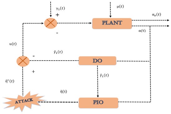
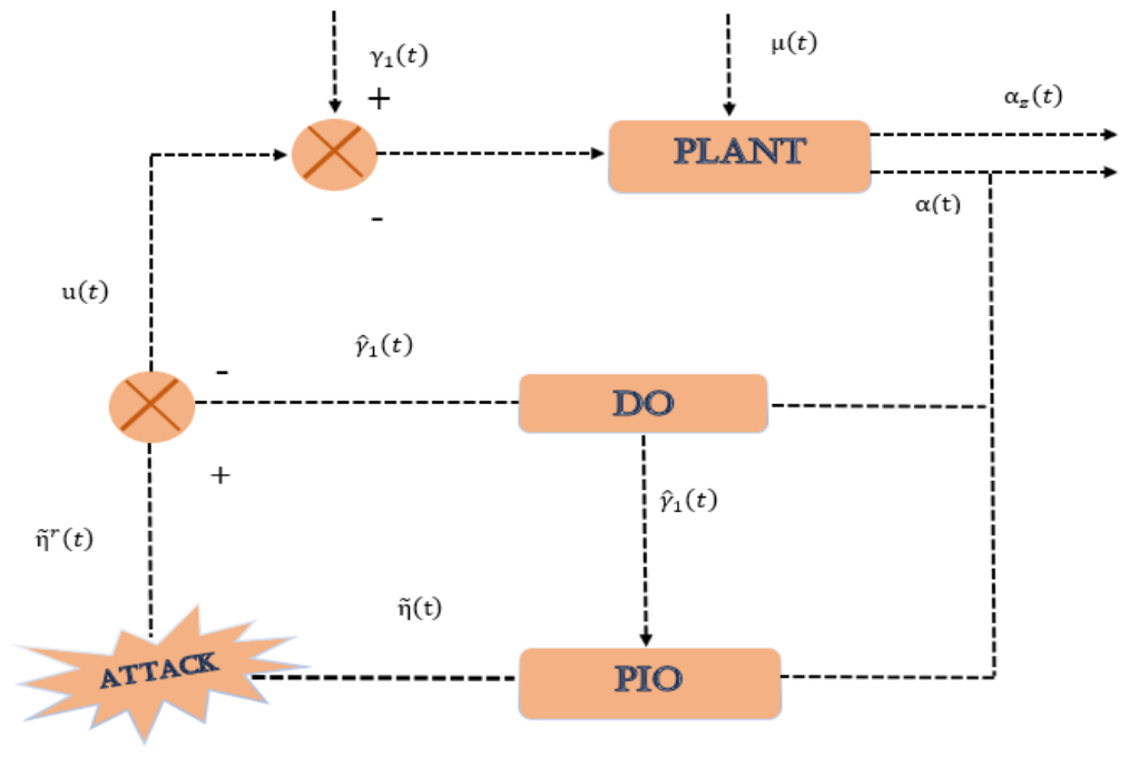
Moreover, a schematic representation of the proposed methodology is provided in Figure 1. Next, by incorporating the designed controller (11) into the systems (3), (6) and defining the estimation errors as $\tilde{\omega }\left(t\right)=\omega \left(t\right)-\widehat{\omega }\left(t\right)$, $\tilde{\eta }\left(t\right)=\widehat{\eta }\left(t\right)-\eta \left(t\right)$, we obtain

$$\begin{array}{c}\hfill \left\{\begin{array}{cc}\dot{\eta }\left(t\right)=\hfill & \mathcal{A}\eta \left(t\right)+\psi \left(t\right)(1-\nu \left(t\right))\mathcal{B}\mathcal{K}\eta \left(t\right)+\psi \left(t\right)(1-\nu \left(t\right))\mathcal{B}\mathcal{K}\tilde{\eta }\left(t\right)+\psi \left(t\right)\nu \left(t\right)\mathcal{B}\mathcal{K}◊\left(t\right)\beta \left(\widehat{\eta }\left(t\right)\right)\hfill \\ \hfill & +(1-\psi \left(t\right))\mathcal{B}\mathcal{K}\eta (t-\varkappa \left(t\right))+(1-\psi \left(t\right))\mathcal{B}\mathcal{K}\tilde{\eta }(t-\varkappa \left(t\right))+\mathcal{B}\mathcal{V}\tilde{\omega }\left(t\right)+\mathcal{D}\mu \left(t\right),\hfill \\ \dot{\tilde{\omega }}\left(t\right)=\hfill & (\mathcal{T}+\mathcal{M}\mathcal{C}\mathcal{B}\mathcal{V})\tilde{\omega }\left(t\right)+\mathcal{U}{\gamma }_2\left(t\right)+\mathcal{M}\mathcal{C}\mathcal{D}\mu \left(t\right),\hfill \\ \dot{\tilde{\eta }}\left(t\right)=\hfill & (\mathcal{A}-{\mathcal{E}}_1\mathcal{C})\tilde{\eta }\left(t\right)-\mathcal{B}\mathcal{V}\tilde{\omega }\left(t\right)+\mathcal{B}\iota \left(t\right)-\mathcal{D}\mu \left(t\right),\hfill \\ \dot{\iota }\left(t\right)=\hfill & -\iota \left(t\right)-{\mathcal{E}}_2\mathcal{C}\tilde{\eta }\left(t\right).\hfill \end{array}\right.\end{array}$$

(12)

Figure 1. Schematic overview of the presented methodology.

Primary Objective: Designing an ARLFC framework that combines output-reliant DO and PIO mechanisms to guarantee FTB for HWDPSs in the presence of hybrid cyber attacks and multiple disturbances.

2.5. Preliminaries

In the final portion of this section, we are going to provide the assumption and definitions that facilitate the core findings of this work.

Assumption 1.

The attack function $l_g\left(\widehat{\eta }\left(t\right)\right)$ adheres to $\Vert l_g\left(\widehat{\eta }\left(t\right)\right)\Vert \le \Vert {\mathcal{J}}_g\widehat{\eta }\left(t\right)\Vert$, for real matrices ${\mathcal{J}}_g$, $g=1,2,\dots ,m.$

Assumption 2.

For some positive scalar $\mathfrak{w}$, the condition ${\int }_0^{\mathsf{T}}{\overline{\mu }}^T\left(t\right)\overline{\mu }\left(t\right)dt\le \mathfrak{w}$ holds with $\overline{\mu }\left(t\right)=\mathrm{col}\{\mu \left(t\right),{\gamma }_2\left(t\right)\}.$

Lemma 1

([46]). Consider matrices $\mathfrak{A}\in {\mathbb{R}}_{\eta }^{+}$ and $\mathfrak{C}\in {\mathbb{R}}^{\eta \times \eta }$ satisfying

$$\left[\begin{array}{cc}\mathfrak{A}& \mathfrak{C}\\ *& \mathfrak{A}\end{array}\right]\ge 0.$$

Let $y,z$ be scalars with $y>z$, and let $\eta :[t-y,t-z]\to {\mathbb{R}}^{\eta }$ be a differentiable function with derivative $\dot{\eta }\left(t\right)$. Then, for any $\mathfrak{f}\left(t\right)\in [z,y]$, the following relation holds:

$$-(y-z){\int }_{t-y}^{t-z}{\dot{\eta }}^T\left(s\right)\mathfrak{A}\dot{\eta }\left(s\right)ds\le {\left[\begin{array}{c}\eta (t-z)\\ \eta (t-\mathfrak{f}(t\left)\right)\\ \eta (t-y)\end{array}\right]}^T\left[\begin{array}{ccc}-\mathfrak{A}& \mathfrak{A}-\mathfrak{C}& \mathfrak{C}\\ *& -2\mathfrak{A}+\mathfrak{C}+{\mathfrak{C}}^T& \mathfrak{A}-\mathfrak{C}\\ *& *& -\mathfrak{A}\end{array}\right]\left[\begin{array}{c}\eta (t-z)\\ \eta (t-\mathfrak{f}(t\left)\right)\\ \eta (t-y)\end{array}\right].$$

Definition 1

([43]). Under Assumption 2, the closed-loop system (12) is finite-time bounded with regard to $({\varrho }_1,{\varrho }_2,\mathsf{T},\overline{\mathcal{Y}},\mathfrak{w})$ if

$$\mathbb{E}\left\{\underset{-\widehat{\varkappa }\le s\le 0}{\sup }\left\{{\chi }^T\left(s\right)\overline{\mathcal{Y}}\chi \left(s\right),{\dot{\chi }}^T\left(s\right)\overline{\mathcal{Y}}\dot{\chi }\left(s\right)\right\}\right\}\le {\varrho }_1\Rightarrow \mathbb{E}\left\{{\chi }^T\left(t\right)\overline{\mathcal{Y}}\chi \left(t\right)\right\}<{\varrho }_2,$$

where ${\varrho }_1>0$ and ${\varrho }_2>0$ are scalars satisfying ${\varrho }_1<{\varrho }_2$, $\overline{\mathcal{Y}}=\mathrm{diag}\{\mathcal{Y},{\mathcal{Y}}_1,{\mathcal{Y}}_2,{\mathcal{Y}}_3\}>0$, and ${\chi }^T\left(t\right)=\left[\begin{array}{cccc}{\eta }^T\left(t\right)& {\tilde{\eta }}^T\left(t\right)& {\tilde{\omega }}^T\left(t\right)& {\iota }^T\left(t\right)\end{array}\right].$

Definition 2

([12]). Let the matrices ${\mathcal{F}}_1\le 0$, ${\mathcal{F}}_2$, ${\mathcal{F}}_3={\mathcal{F}}_3^T$ and a parameter $\epsilon >0$ be given. The closed-loop system (12) is said to be strictly $({\mathcal{F}}_1,{\mathcal{F}}_2,{\mathcal{F}}_3)$-ε dissipative under zero initial conditions if, for any $\mathsf{T}>0$ and for all $\overline{\mu }\left(t\right)\in L_2[0,+\infty )$, the following criterion holds:

$$\mathbb{E}\left\{{\int }_0^{\mathsf{T}}\left({\alpha }_z^T\left(g\right){\mathcal{F}}_1{\alpha }_z\left(g\right)+2{\alpha }_z^T\left(g\right){\mathcal{F}}_2\overline{\mu }\left(g\right)+{\overline{\mu }}^T\left(g\right)({\mathcal{F}}_3-\epsilon I)\overline{\mu }\left(g\right)\right)dg\right\}\ge 0.$$

3. Main Results

This section focuses on dealing with the disturbance rejection and FTB issue for the explored HWDPSs (3) relying on the designed DO-driven ARLFC protocol (11). Specifically, within the realm of linear matrix inequalities, we acquire sufficient requirements for assuring the intended stability of the closed-loop system (12). This is accomplished by selecting an appropriate Lyapunov function.

Theorem 1.

Let the Assumptions 1 and 2 hold. Assume that the scalars $\{{\overline{\varphi }}_g,\overline{\nu },\overline{\psi }\}\in [0,1]$, $\widehat{\varkappa }>0$, $\mathfrak{z}>0$ and built controller gain matrix $\mathcal{K}$, configured observer gain matrices $\mathcal{M}$, ${\mathcal{E}}_1$, ${\mathcal{E}}_2$ are defined beforehand. Then, the considered system (3) is finite-time bounded under the ARLFC (11), if the matrices $\{\mathfrak{M},\mathfrak{N},\mathfrak{Q},\mathfrak{R},\mathfrak{S},\mathfrak{T},\mathfrak{Z}\}\in {\mathbb{R}}_{\eta }^{+}$, $\mathfrak{O}\in {\mathbb{R}}_{\omega }^{+}$ and $\mathfrak{P}\in {\mathbb{R}}_u^{+}$, $\{\mathfrak{Y},{\mathfrak{R}}_1,{\mathfrak{R}}_2\}\in {\mathbb{R}}^{\eta \times \eta }$ exist, such that the requirements specified below are met:

$$\begin{array}{c}\hfill \left[\begin{array}{cc}\mathfrak{S}& {\mathfrak{R}}_1\\ *& \mathfrak{S}\end{array}\right]>0,\left[\begin{array}{cc}\mathfrak{T}& {\mathfrak{R}}_2\\ *& \mathfrak{T}\end{array}\right]>0,\end{array}$$

(13)

$$\begin{array}{c}\hfill \left[\mathsf{\aleph }\right]<0,\end{array}$$

(14)

$$\begin{array}{c}\hfill \left(\delta {\varrho }_1+\mathfrak{z}\mathfrak{w}\right)<e^{-\mathfrak{z}\mathsf{T}}{\varsigma }_1{\varrho }_2,\end{array}$$

(15)

where

$$\begin{array}{cc}\hfill \left[\mathsf{\aleph }\right]=& {\left[\mathsf{\aleph }\right]}_a+{\left[\mathsf{\aleph }\right]}_b,\hfill \\ \hfill {\left[\mathsf{\aleph }\right]}_a=& {\mathsf{\aleph }}^1+{\mathsf{\aleph }}^4+{\mathsf{\aleph }}^5+{\mathsf{\aleph }}^6+{\mathsf{\aleph }}^7+{\mathsf{\aleph }}^{10}+{\mathsf{\aleph }}^{11},\hfill \\ \hfill {\left[\mathsf{\aleph }\right]}_b=& {\mathsf{\aleph }}^2+{\mathsf{\aleph }}^3+{\mathsf{\aleph }}^8+{\mathsf{\aleph }}^9+{\mathsf{\aleph }}^{12},\hfill \\ \hfill {\mathsf{\aleph }}^1=& sym\left\{{\mathfrak{r}}_1^T\mathfrak{M}{\mathfrak{r}}_2+{\mathfrak{r}}_3^T\mathfrak{N}{\mathfrak{r}}_4\right\},\hfill \\ \hfill {\mathsf{\aleph }}^2=& sym\left\{{\mathfrak{r}}_6^T\mathfrak{O}\left((\mathcal{T}+\mathcal{M}\mathcal{C}\mathcal{B}\mathcal{V}){\mathfrak{r}}_6+\mathcal{U}{\mathfrak{r}}_{13}+\mathcal{M}\mathcal{C}\mathcal{D}{\mathfrak{r}}_{12}\right)\right\},\hfill \\ \hfill {\mathsf{\aleph }}^3=& sym\left\{{\mathfrak{r}}_5^T\mathfrak{P}\left(-{\mathfrak{r}}_5-{\mathcal{E}}_2\mathcal{C}{\mathfrak{r}}_3\right)\right\},\hfill \\ \hfill {\mathsf{\aleph }}^4=& {\mathfrak{r}}_1^T\mathfrak{Q}{\mathfrak{r}}_1-{\mathfrak{r}}_9^T\mathfrak{Q}{\mathfrak{r}}_9+{\mathfrak{r}}_3^T\mathfrak{R}{\mathfrak{r}}_3-{\mathfrak{r}}_{10}^T\mathfrak{R}{\mathfrak{r}}_{10},\hfill \\ \hfill {\mathsf{\aleph }}^5=& {\mathfrak{r}}_2^T{\widehat{\varkappa }}^2\mathfrak{S}{\mathfrak{r}}_2+{\mathfrak{r}}_4^T{\widehat{\varkappa }}^2\mathfrak{T}{\mathfrak{r}}_4,\hfill \\ \hfill {\mathsf{\aleph }}^6=& -{\mathfrak{r}}_1^T\mathfrak{S}{\mathfrak{r}}_1+sym\left\{{\mathfrak{r}}_1^T(\mathfrak{S}-{\mathfrak{R}}_1){\mathfrak{r}}_7+{\mathfrak{r}}_1^T{\mathfrak{R}}_1{\mathfrak{r}}_9+{\mathfrak{r}}_7^T(\mathfrak{S}-{\mathfrak{R}}_1){\mathfrak{r}}_9\right\}+{\mathfrak{r}}_7^T(-2\mathfrak{S}+{\mathfrak{R}}_1+{\mathfrak{R}}_1^T){\mathfrak{r}}_7-{\mathfrak{r}}_9^T\mathfrak{S}{\mathfrak{r}}_9,\hfill \\ \hfill {\mathsf{\aleph }}^7=& -{\mathfrak{r}}_3^T\mathfrak{T}{\mathfrak{r}}_3+sym\left\{{\mathfrak{r}}_3^T(\mathfrak{T}-{\mathfrak{R}}_2){\mathfrak{r}}_8+{\mathfrak{r}}_3^T{\mathfrak{R}}_2{\mathfrak{r}}_{10}+{\mathfrak{r}}_8^T(\mathfrak{T}-{\mathfrak{R}}_2){\mathfrak{r}}_{10}\right\}+{\mathfrak{r}}_8^T(-2\mathfrak{T}+{\mathfrak{R}}_2+{\mathfrak{R}}_2^T){\mathfrak{r}}_8-{\mathfrak{r}}_{10}^T\mathfrak{T}{\mathfrak{r}}_{10},\hfill \\ \hfill {\mathsf{\aleph }}^8=& sym\left\{\left[{\mathfrak{r}}_1^T{\mathfrak{m}}_1+{\mathfrak{r}}_2^T{\mathfrak{m}}_2\right]\mathfrak{Y}\right[\mathcal{A}{\mathfrak{r}}_1+\overline{\psi }(1-\overline{\nu })\mathcal{B}\mathcal{K}{\mathfrak{r}}_1+\overline{\psi }(1-\overline{\nu })\mathcal{B}\mathcal{K}{\mathfrak{r}}_3+\overline{\psi }\overline{\nu }\mathcal{B}\mathcal{K}\overline{◊}{\mathfrak{r}}_{11}\hfill \\ \hfill & +(1-\overline{\psi })\mathcal{B}\mathcal{K}{\mathfrak{r}}_7+(1-\overline{\psi })\mathcal{B}\mathcal{K}{\mathfrak{r}}_8+\mathcal{B}\mathcal{V}{\mathfrak{r}}_6+\mathcal{D}{\mathfrak{r}}_{12}-{\mathfrak{r}}_2\left]\right\},\hfill \\ \hfill {\mathsf{\aleph }}^9=& sym\left\{\left[{\mathfrak{r}}_3^T{\mathfrak{n}}_1+{\mathfrak{r}}_4^T{\mathfrak{n}}_2\right]\mathfrak{Z}\left[(\mathcal{A}-{\mathcal{E}}_1\mathcal{C}){\mathfrak{r}}_3-\mathcal{B}\mathcal{V}{\mathfrak{r}}_6+\mathcal{B}{\mathfrak{r}}_5-\mathcal{D}{\mathfrak{r}}_{12}-{\mathfrak{r}}_4\right]\right\},\hfill \\ \hfill {\mathsf{\aleph }}^{10}=& [{\mathfrak{r}}_1^T+{\mathfrak{r}}_3^T]{\displaystyle \sum _{g=1}^m}{\mathcal{J}}_g^T{\mathcal{J}}_g[{\mathfrak{r}}_1+{\mathfrak{r}}_3]-{\mathfrak{r}}_{11}^T{\mathfrak{r}}_{11},\hfill \\ \hfill {\mathsf{\aleph }}^{11}=& -{\mathfrak{r}}_1^T\mathfrak{z}\mathfrak{M}{\mathfrak{r}}_1-{\mathfrak{r}}_3^T\mathfrak{z}\mathfrak{N}{\mathfrak{r}}_3-{\mathfrak{r}}_5^T\mathfrak{z}\mathfrak{P}{\mathfrak{r}}_5-{\mathfrak{r}}_6^T\mathfrak{z}\mathfrak{O}{\mathfrak{r}}_6,\hfill \\ \hfill {\mathsf{\aleph }}^{12}=& -{\mathfrak{r}}_{12}^T\mathfrak{z}{\mathfrak{r}}_{12}-{\mathfrak{r}}_{13}^T\mathfrak{z}{\mathfrak{r}}_{13},\hfill \\ \hfill \delta =& {\varsigma }_2+{\varsigma }_3+{\varsigma }_4+{\varsigma }_5+\widehat{\varkappa }{\varsigma }_6+\widehat{\varkappa }{\varsigma }_7+{\displaystyle \frac{{\widehat{\varkappa }}^3}{2}}{\varsigma }_8+{\displaystyle \frac{{\widehat{\varkappa }}^3}{2}}{\varsigma }_9,\hfill \\ \hfill {\varsigma }_1=& {\lambda }_{min}\left(\widetilde{\widehat{\mathfrak{M}}}\right),{\varsigma }_2={\lambda }_{max}\left(\tilde{\mathfrak{M}}\right),{\varsigma }_3={\lambda }_{max}\left(\tilde{\mathfrak{N}}\right),{\varsigma }_4={\lambda }_{max}\left(\tilde{\mathfrak{O}}\right),{\varsigma }_5={\lambda }_{max}\left(\tilde{\mathfrak{P}}\right),\hfill \\ \hfill {\varsigma }_6=& {\lambda }_{max}\left(\tilde{\mathfrak{Q}}\right),{\varsigma }_7={\lambda }_{max}\left(\tilde{\mathfrak{R}}\right),{\varsigma }_8={\lambda }_{max}\left(\tilde{\mathfrak{S}}\right),{\varsigma }_9={\lambda }_{max}\left(\tilde{\mathfrak{T}}\right),\hfill \\ \hfill {\mathfrak{r}}_c=& \left[\begin{array}{ccc}{0}_{d_c\times {\sum }_{j=1}^{c-1}{d}_j}& I_{d_c}& 0_{d_c\times {\sum }_{j=c+1}^{13}{d}_j}\end{array}\right],c=1,2,\dots ,13,\hfill \\ \hfill & (d_1,d_2,\dots ,d_{13})=(\eta ,\eta ,\eta ,\eta ,u,\omega ,\eta ,\eta ,\eta ,\eta ,m\eta ,\mu ,\gamma ).\hfill \end{array}$$

Proof. 

The Lyapunov stability theory is employed in pursuit of the foremost goal of this section. Thus, we put forward the Lyapunov function in the following form:

$$\mathcal{L}\left(t\right)={\mathcal{L}}_1\left(t\right)+{\mathcal{L}}_2\left(t\right)+{\mathcal{L}}_3\left(t\right),$$

(16)

where

$$\begin{array}{cc}\hfill {\mathcal{L}}_1\left(t\right)=& {\eta }^T\left(t\right)\mathfrak{M}\eta \left(t\right)+{\tilde{\eta }}^T\left(t\right)\mathfrak{N}\tilde{\eta }\left(t\right)+{\tilde{\omega }}^T\left(t\right)\mathfrak{O}\tilde{\omega }\left(t\right)+{\iota }^T\left(t\right)\mathfrak{P}\iota \left(t\right),\hfill \end{array}$$

(17)

$$\begin{array}{cc}\hfill {\mathcal{L}}_2\left(t\right)=& {\int }_{t-\widehat{\varkappa }}^t{\eta }^T\left(s\right)\mathfrak{Q}\eta \left(s\right)ds+{\int }_{t-\widehat{\varkappa }}^t{\tilde{\eta }}^T\left(s\right)\mathfrak{R}\tilde{\eta }\left(s\right)ds,\hfill \end{array}$$

(18)

$$\begin{array}{cc}\hfill {\mathcal{L}}_3\left(t\right)=& \widehat{\varkappa }{\int }_{-\widehat{\varkappa }}^0{\int }_{t+q}^t{\dot{\eta }}^T\left(s\right)\mathfrak{S}\dot{\eta }\left(s\right)dsdq+\widehat{\varkappa }{\int }_{-\widehat{\varkappa }}^0{\int }_{t+q}^t{\dot{\tilde{\eta }}}^T\left(s\right)\mathfrak{T}\dot{\tilde{\eta }}\left(s\right)dsdq.\hfill \end{array}$$

(19)

By differentiating the constructed Lyapunov function with respect to time t, in conjunction with the system (12) and taking mathematical expectation on both sides, we secure the resultant expression:

$$\begin{array}{cc}\hfill \mathbb{E}\left\{{\dot{\mathcal{L}}}_1\left(t\right)\right\}=& \mathbb{E}\{{\eta }^T\left(t\right)\mathfrak{M}\dot{\eta }\left(t\right)+{\dot{\eta }}^T\left(t\right)\mathfrak{M}\eta \left(t\right)+{\tilde{\eta }}^T\left(t\right)\mathfrak{N}\dot{\tilde{\eta }}\left(t\right)+{\dot{\tilde{\eta }}}^T\left(t\right)\mathfrak{N}\tilde{\eta }\left(t\right)\hfill \\ \hfill & +{\tilde{\omega }}^T\left(t\right)\mathfrak{O}\left((\mathcal{T}+\mathcal{M}\mathcal{C}\mathcal{B}\mathcal{V})\tilde{\omega }\left(t\right)+\mathcal{U}{\gamma }_2\left(t\right)+\mathcal{M}\mathcal{C}\mathcal{D}\mu \left(t\right)\right)\hfill \\ \hfill & +{\left((\mathcal{T}+\mathcal{M}\mathcal{C}\mathcal{B}\mathcal{V})\tilde{\omega }\left(t\right)+\mathcal{U}{\gamma }_2\left(t\right)+\mathcal{M}\mathcal{C}\mathcal{D}\mu \left(t\right)\right)}^T\mathfrak{O}\tilde{\omega }\left(t\right)\hfill \\ \hfill & +{\iota }^T\left(t\right)\mathfrak{P}\left(-\iota \left(t\right)-{\mathcal{E}}_2\mathcal{C}\tilde{\eta }\left(t\right)\right)+{\left(-\iota \left(t\right)-{\mathcal{E}}_2\mathcal{C}\tilde{\eta }\left(t\right)\right)}^T\mathfrak{P}\iota \left(t\right)\}\hfill \\ \hfill =& \mathbb{E}\left\{{\mathfrak{a}}^T\left(t\right)({\mathsf{\aleph }}^1+{\mathsf{\aleph }}^2+{\mathsf{\aleph }}^3)\mathfrak{a}\left(t\right)\right\},\hfill \end{array}$$

(20)

$$\begin{array}{cc}\hfill \mathbb{E}\left\{{\dot{\mathcal{L}}}_2\left(t\right)\right\}=& \mathbb{E}\{{\eta }^T\left(t\right)\mathfrak{Q}\eta \left(t\right)-{\eta }^T(t-\widehat{\varkappa })\mathfrak{Q}\eta (t-\widehat{\varkappa })+{\tilde{\eta }}^T\left(t\right)\mathfrak{R}\tilde{\eta }\left(t\right)\hfill \\ \hfill & -{\tilde{\eta }}^T(t-\widehat{\varkappa })\mathfrak{R}\tilde{\eta }(t-\widehat{\varkappa })\}=\mathbb{E}\left\{{\mathfrak{a}}^T\left(t\right){\mathsf{\aleph }}^4\mathfrak{a}\left(t\right)\right\},\hfill \end{array}$$

(21)

$$\begin{array}{cc}\hfill \mathbb{E}\left\{{\dot{\mathcal{L}}}_3\left(t\right)\right\}=& \mathbb{E}\{{\widehat{\varkappa }}^2{\dot{\eta }}^T\left(t\right)\mathfrak{S}\dot{\eta }\left(t\right)+{\widehat{\varkappa }}^2{\dot{\tilde{\eta }}}^T\left(t\right)\mathfrak{T}\dot{\tilde{\eta }}\left(t\right)-\widehat{\varkappa }{\int }_{t-\widehat{\varkappa }}^t{\dot{\eta }}^T\left(s\right)\mathfrak{S}\dot{\eta }\left(s\right)ds\hfill \\ \hfill & -\widehat{\varkappa }{\int }_{t-\widehat{\varkappa }}^t{\dot{\tilde{\eta }}}^T\left(s\right)\mathfrak{T}\dot{\tilde{\eta }}\left(s\right)ds\}\hfill \\ \hfill =& \mathbb{E}\left\{{\mathfrak{a}}^T\left(t\right){\mathsf{\aleph }}^5\mathfrak{a}\left(t\right)-\widehat{\varkappa }{\int }_{t-\widehat{\varkappa }}^t{\dot{\eta }}^T\left(s\right)\mathfrak{S}\dot{\eta }\left(s\right)ds-\widehat{\varkappa }{\int }_{t-\widehat{\varkappa }}^t{\dot{\tilde{\eta }}}^T\left(s\right)\mathfrak{T}\dot{\tilde{\eta }}\left(s\right)ds\right\}.\hfill \end{array}$$

(22)

By applying Lemma 1 to the integral terms in the above equation, we obtain the following inequalities under the conditions (13):

$$\begin{array}{cc}\hfill -\widehat{\varkappa }{\int }_{t-\widehat{\varkappa }}^t{\dot{\eta }}^T\left(s\right)\mathfrak{S}\dot{\eta }\left(s\right)ds\le & {\left[\begin{array}{c}\eta \left(t\right)\\ \eta (t-\varkappa (t\left)\right)\\ \eta (t-\widehat{\varkappa })\end{array}\right]}^T\left[\begin{array}{ccc}-\mathfrak{S}& \mathfrak{S}-{\mathfrak{R}}_1& {\mathfrak{R}}_1\\ *& -2\mathfrak{S}+{\mathfrak{R}}_1+{\mathfrak{R}}_1^T& \mathfrak{S}-{\mathfrak{R}}_1\\ *& *& -\mathfrak{S}\end{array}\right]\left[\begin{array}{c}\eta \left(t\right)\\ \eta (t-\varkappa (t\left)\right)\\ \eta (t-\widehat{\varkappa })\end{array}\right]\hfill \\ \hfill =& {\mathfrak{a}}^T\left(t\right){\mathsf{\aleph }}^6\mathfrak{a}\left(t\right),\hfill \end{array}$$

(23)

$$\begin{array}{cc}\hfill -\widehat{\varkappa }{\int }_{t-\widehat{\varkappa }}^t{\dot{\tilde{\eta }}}^T\left(s\right)\mathfrak{T}\dot{\tilde{\eta }}\left(s\right)ds\le & {\left[\begin{array}{c}\tilde{\eta }\left(t\right)\\ \tilde{\eta }(t-\varkappa \left(t\right))\\ \tilde{\eta }(t-\widehat{\varkappa })\end{array}\right]}^T\left[\begin{array}{ccc}-\mathfrak{T}& \mathfrak{T}-{\mathfrak{R}}_2& {\mathfrak{R}}_2\\ *& -2\mathfrak{T}+{\mathfrak{R}}_2+{\mathfrak{R}}_2^T& \mathfrak{T}-{\mathfrak{R}}_2\\ *& *& -\mathfrak{T}\end{array}\right]\left[\begin{array}{c}\tilde{\eta }\left(t\right)\\ \tilde{\eta }(t-\varkappa \left(t\right))\\ \tilde{\eta }(t-\widehat{\varkappa })\end{array}\right]\hfill \\ \hfill =& {\mathfrak{a}}^T\left(t\right){\mathsf{\aleph }}^7\mathfrak{a}\left(t\right).\hfill \end{array}$$

(24)

Moreover, the following zero equations are introduced to aid the analysis for some real matrices $\mathfrak{Y}$, $\mathfrak{Z}$ and positive scalars ${\mathfrak{m}}_1$, ${\mathfrak{m}}_2$, ${\mathfrak{n}}_1$, ${\mathfrak{n}}_2$:

$$\begin{array}{cc}\hfill 0=& \mathbb{E}\left\{2{\left[\eta \left(t\right){\mathfrak{m}}_1+\dot{\eta }\left(t\right){\mathfrak{m}}_2\right]}^T\mathfrak{Y}\right[\mathcal{A}\eta \left(t\right)+\psi \left(t\right)(1-\nu \left(t\right))\mathcal{B}\mathcal{K}\eta \left(t\right)+\psi \left(t\right)(1-\nu \left(t\right))\mathcal{B}\mathcal{K}\tilde{\eta }\left(t\right)\hfill \\ \hfill & +\psi \left(t\right)\nu \left(t\right)\mathcal{B}\mathcal{K}◊\left(t\right)\beta \left(\widehat{\eta }\left(t\right)\right)+(1-\psi \left(t\right))\mathcal{B}\mathcal{K}\eta (t-\varkappa \left(t\right))+(1-\psi \left(t\right))\mathcal{B}\mathcal{K}\tilde{\eta }(t-\varkappa \left(t\right))\hfill \\ \hfill & +\mathcal{B}\mathcal{V}\tilde{\omega }\left(t\right)+\mathcal{D}\mu \left(t\right)-\dot{\eta }\left(t\right)\left]\right\},\hfill \\ \hfill =& \mathbb{E}\left\{{\mathfrak{a}}^T\left(t\right){\mathsf{\aleph }}^8\mathfrak{a}\left(t\right)\right\},\hfill \end{array}$$

(25)

$$\begin{array}{cc}\hfill 0=& \mathbb{E}\left\{2{\left[\tilde{\eta }\left(t\right){\mathfrak{n}}_1+\dot{\tilde{\eta }}\left(t\right){\mathfrak{n}}_2\right]}^T\mathfrak{Z}\left[(\mathcal{A}-{\mathcal{E}}_1\mathcal{C})\tilde{\eta }\left(t\right)-\mathcal{B}\mathcal{V}\tilde{\omega }\left(t\right)+\mathcal{B}\iota \left(t\right)-\mathcal{D}\mu \left(t\right)-\dot{\tilde{\eta }}\left(t\right)\right]\right\},\hfill \\ \hfill =& \mathbb{E}\left\{{\mathfrak{a}}^T\left(t\right){\mathsf{\aleph }}^9\mathfrak{a}\left(t\right)\right\}.\hfill \end{array}$$

(26)

Furthermore, based on Assumption 1, the following equation is obtained:

$$\begin{array}{cc}\hfill 0\le & {\widehat{\eta }}^T\left(t\right){\displaystyle \sum _{g=1}^m}{\mathcal{J}}_g^T{\mathcal{J}}_g\widehat{\eta }\left(t\right)-{\beta }^T\left(\widehat{\eta }\left(t\right)\right)\beta \left(\widehat{\eta }\left(t\right)\right)\hfill \\ \hfill 0\le & [{\eta }^T\left(t\right)+{\tilde{\eta }}^T\left(t\right)]{\displaystyle \sum _{g=1}^m}{\mathcal{J}}_g^T{\mathcal{J}}_g[\eta \left(t\right)+\tilde{\eta }\left(t\right)]-{\beta }^T\left(\widehat{\eta }\left(t\right)\right)\beta \left(\widehat{\eta }\left(t\right)\right)\hfill \\ \hfill =& {\mathfrak{a}}^T\left(t\right){\mathsf{\aleph }}^{10}\mathfrak{a}\left(t\right).\hfill \end{array}$$

(27)

Next, using the preceding relations (20)–(27), we obtain the following inequality:

$$\mathbb{E}\left\{\dot{\mathcal{L}}\left(t\right)--\mathfrak{z}\mathcal{L}\left(t\right)-{\overline{\mu }}^T\left(t\right)\mathfrak{z}\overline{\mu }\left(t\right)\right\}\le \mathbb{E}\left\{{\mathfrak{a}}^T\left(t\right)\left[\mathsf{\aleph }\right]\mathfrak{a}\left(t\right)\right\},$$

(28)

where ${\mathfrak{a}}^T\left(t\right)=[{\eta }^T\left(t\right){\dot{\eta }}^T\left(t\right){\tilde{\eta }}^T\left(t\right){\dot{\tilde{\eta }}}^T\left(t\right){\iota }^T\left(t\right){\tilde{\omega }}^T\left(t\right){\eta }^T(t-\varkappa \left(t\right)){\tilde{\eta }}^T(t-\varkappa \left(t\right))$ ${\eta }^T(t-\widehat{\varkappa }){\tilde{\eta }}^T(t-\widehat{\varkappa }){\beta }^T\left(\widehat{\eta }\left(t\right)\right){\mu }^T\left(t\right){\gamma }_2^T\left(t\right)]$ and $\left[\mathsf{\aleph }\right]$ is defined in theorem statement. Furthermore, if the relation (14) holds then it can be asserted that

$$\mathbb{E}\left\{\dot{\mathcal{L}}\left(t\right)-\mathfrak{z}\mathcal{L}\left(t\right)-{\overline{\mu }}^T\left(t\right)\mathfrak{z}\overline{\mu }\left(t\right)\right\}\le \mathbb{E}\left\{{\mathfrak{a}}^T\left(t\right)\left[\mathsf{\aleph }\right]\mathfrak{a}\left(t\right)\right\}<0,$$

(29)

where ${\overline{\mu }}^T\left(t\right)=\left[{\mu }^T\left(t\right){\gamma }_2^T\left(t\right)\right]$.

From the above relation, the following relation is deduced:

$$\mathbb{E}\left\{\dot{\mathcal{L}}\left(t\right)-\mathfrak{z}\mathcal{L}\left(t\right)\right\}<\mathbb{E}\left\{{\overline{\mu }}^T\left(t\right)\mathfrak{z}\overline{\mu }\left(t\right)\right\}.$$

(30)

Next, we multiply both sides of inequality (30) by the exponential function $e^{-\mathfrak{z}t}$ and integrate over $[0,t]$. Using $e^{-\mathfrak{z}s}\le 1$, $t\le \mathsf{T}$, and Assumption 2, we obtain

$$\begin{array}{cc}\hfill \mathbb{E}\left\{\mathcal{L}\left(t\right)\right\}& <e^{\mathfrak{z}t}\left[\mathbb{E}\left\{\mathcal{L}\left(0\right)\right\}+\mathfrak{z}{\int }_0^t{e}^{-\mathfrak{z}s}\mathbb{E}\left\{{\overline{\mu }}^T\left(s\right)\overline{\mu }\left(s\right)\right\}ds\right]\hfill \\ & \le e^{\mathfrak{z}\mathsf{T}}\left[\mathbb{E}\left\{\mathcal{L}\left(0\right)\right\}+\mathfrak{z}\mathfrak{w}\right].\hfill \end{array}$$

(31)

Define $\tilde{\mathfrak{M}}={\mathcal{Y}}^{-{\displaystyle \frac{1}{2}}}\mathfrak{M}{\mathcal{Y}}^{-{\displaystyle \frac{1}{2}}}$, $\tilde{\mathfrak{N}}={\mathcal{Y}}_1^{-{\displaystyle \frac{1}{2}}}\mathfrak{N}{\mathcal{Y}}_1^{-{\displaystyle \frac{1}{2}}}$, $\tilde{\mathfrak{O}}={\mathcal{Y}}_2^{-{\displaystyle \frac{1}{2}}}\mathfrak{O}{\mathcal{Y}}_2^{-{\displaystyle \frac{1}{2}}}$, $\tilde{\mathfrak{P}}={\mathcal{Y}}_3^{-{\displaystyle \frac{1}{2}}}\mathfrak{P}{\mathcal{Y}}_3^{-{\displaystyle \frac{1}{2}}}$, $\tilde{\mathfrak{Q}}={\mathcal{Y}}^{-{\displaystyle \frac{1}{2}}}\mathfrak{Q}{\mathcal{Y}}^{-{\displaystyle \frac{1}{2}}}$, $\tilde{\mathfrak{R}}={\mathcal{Y}}_1^{-{\displaystyle \frac{1}{2}}}\mathfrak{R}{\mathcal{Y}}_1^{-{\displaystyle \frac{1}{2}}}$, $\tilde{\mathfrak{S}}={\mathcal{Y}}^{-{\displaystyle \frac{1}{2}}}\mathfrak{S}{\mathcal{Y}}^{-{\displaystyle \frac{1}{2}}}$, $\tilde{\mathfrak{T}}={\mathcal{Y}}_1^{-{\displaystyle \frac{1}{2}}}\mathfrak{T}{\mathcal{Y}}_1^{-{\displaystyle \frac{1}{2}}}$ and $\widehat{\mathfrak{M}}=diag\{\mathfrak{M},\mathfrak{N},\mathfrak{O},\mathfrak{P}\}$, $\widetilde{\widehat{\mathfrak{M}}}={\overline{\mathcal{Y}}}^{-{\displaystyle \frac{1}{2}}}\widehat{\mathfrak{M}}{\overline{\mathcal{Y}}}^{-{\displaystyle \frac{1}{2}}}$. Based on these relations, we can establish the following connection:

$$\begin{array}{cc}\hfill \mathbb{E}\left\{\mathcal{L}\left(t\right)\right\}\ge & \mathbb{E}\left\{{\chi }^T\left(t\right)\widehat{\mathfrak{M}}\chi \left(t\right)\right\}=\mathbb{E}\left\{{\chi }^T\left(t\right){\overline{\mathcal{Y}}}^{{\displaystyle \frac{1}{2}}}\widetilde{\widehat{\mathfrak{M}}}{\overline{\mathcal{Y}}}^{{\displaystyle \frac{1}{2}}}\chi \left(t\right)\right\}\hfill \\ \hfill \ge & {\lambda }_{min}\left(\widetilde{\widehat{\mathfrak{M}}}\right)\mathbb{E}\left\{{\chi }^T\left(t\right)\overline{\mathcal{Y}}\chi \left(t\right)\right\}\hfill \\ \hfill =& {\varsigma }_1\mathbb{E}\left\{{\chi }^T\left(t\right)\overline{\mathcal{Y}}\chi \left(t\right)\right\}.\hfill \end{array}$$

(32)

In addition, the following formula can potentially be obtained via Equation (16):

$$\begin{array}{cc}\hfill \mathbb{E}\left\{\mathcal{L}\left(0\right)\right\}=& \mathbb{E}\{{\eta }^T\left(0\right)\mathfrak{M}\eta \left(0\right)+{\tilde{\omega }}^T\left(0\right)\mathfrak{O}\tilde{\omega }\left(0\right)+{\tilde{\eta }}^T\left(0\right)\mathfrak{N}\tilde{\eta }\left(0\right)+{\iota }^T\left(0\right)\mathfrak{P}\iota \left(0\right)\hfill \\ \hfill & +{\int }_{-\widehat{\varkappa }}^0{\eta }^T\left(s\right)\mathfrak{Q}\eta \left(s\right)ds+{\int }_{-\widehat{\varkappa }}^0{\tilde{\eta }}^T\left(s\right)\mathfrak{R}\tilde{\eta }\left(s\right)ds+\widehat{\varkappa }{\int }_{-\widehat{\varkappa }}^0{\int }_q^0{\dot{\eta }}^T\left(s\right)\mathfrak{S}\dot{\eta }\left(s\right)dqds\hfill \\ \hfill & +\widehat{\varkappa }{\int }_{-\widehat{\varkappa }}^0{\int }_q^0{\dot{\tilde{\eta }}}^T\left(s\right)\mathfrak{T}\dot{\tilde{\eta }}\left(s\right)dqds\}\hfill \\ \hfill \le & [{\lambda }_{max}\left(\tilde{\mathfrak{M}}\right)+{\lambda }_{max}\left(\tilde{\mathfrak{N}}\right)+{\lambda }_{max}\left(\tilde{\mathfrak{O}}\right)+{\lambda }_{max}\left(\tilde{\mathfrak{P}}\right)+\widehat{\varkappa }{\lambda }_{max}\left(\tilde{\mathfrak{Q}}\right)+\widehat{\varkappa }{\lambda }_{max}\left(\tilde{\mathfrak{R}}\right)+{\displaystyle \frac{{\widehat{\varkappa }}^3}{2}}{\lambda }_{max}\left(\tilde{\mathfrak{S}}\right)\hfill \\ \hfill & +{\displaystyle \frac{{\widehat{\varkappa }}^3}{2}}{\lambda }_{max}\left(\tilde{\mathfrak{T}}\right)]\mathbb{E}\left\{\underset{-\widehat{\varkappa }\le s\le 0}{\sup }\{{\eta }^T\left(s\right)\mathcal{Y}\eta \left(s\right),{\tilde{\eta }}^T\left(s\right){\mathcal{Y}}_1\tilde{\eta }\left(s\right),{\tilde{\omega }}^T\left(s\right){\mathcal{Y}}_2\tilde{\omega }\left(s\right),{\iota }^T\left(s\right){\mathcal{Y}}_3\iota \left(s\right),{\dot{\eta }}^T\left(s\right)\mathcal{Y}\dot{\eta }\left(s\right),{\dot{\tilde{\eta }}}^T\left(s\right){\mathcal{Y}}_1\dot{\tilde{\eta }}\left(s\right)\}\right\}\hfill \\ \hfill \le & \delta {\varrho }_1.\hfill \end{array}$$

(33)

where $\delta ={\varsigma }_2+{\varsigma }_3+{\varsigma }_4+{\varsigma }_5+\widehat{\varkappa }{\varsigma }_6+\widehat{\varkappa }{\varsigma }_7+{\displaystyle \frac{{\widehat{\varkappa }}^3}{2}}{\varsigma }_8+{\displaystyle \frac{{\widehat{\varkappa }}^3}{2}}{\varsigma }_9$.

Finally, using Equations (30)–(33), we obtain the following relation:

$$\begin{array}{c}\hfill \mathbb{E}\left\{{\chi }^T\left(t\right)\overline{\mathcal{Y}}\chi \left(t\right)\right\}\le {\displaystyle \frac{\mathbb{E}\left\{\mathcal{L}\left(t\right)\right\}}{{\varsigma }_1}}\le e^{\mathfrak{z}\mathsf{T}}{\displaystyle \frac{\left(\delta {\varrho }_1+\mathfrak{z}\mathfrak{w}\right)}{{\varsigma }_1}}.\end{array}$$

(34)

In addition, for any t in the interval $[0,\mathsf{T}]$, we can establish that $\mathbb{E}\left\{{\chi }^T\left(t\right)\overline{\mathcal{Y}}\chi \left(t\right)\right\}<{\varrho }_2$ if (15) is satisfied. Hence, according to Definition 1, we can deduce that the developed ARLFC (11) enables HWDPSs (3) to achieve FTB. With this, we conclude the proof of the theorem.    □

The following result extends Theorem 1 to the case where the observer and controller gain matrices are unknown. In this regard, sufficient requirements for the closed-loop system (12) to be finite-time bounded with respect to strictly $({\mathcal{F}}_1,{\mathcal{F}}_2,{\mathcal{F}}_3)-\epsilon$ dissipative performance are established.

Theorem 2.

Under Assumptions 1, 2 and for given scalars $\{{\overline{\varphi }}_g,\overline{\nu },\overline{\psi }\}\in [0,1]$, $\widehat{\varkappa }>0$, $\mathfrak{z}>0$, the closed-loop system (12) achieves FTB with respect to strictly $({\mathcal{F}}_1,{\mathcal{F}}_2,{\mathcal{F}}_3)-\epsilon$ dissipative performance if there exist a scalar $\mathfrak{e}>0$ and matrices $\{\mathfrak{M},\mathfrak{N},\mathfrak{Q},\mathfrak{R},\mathfrak{S},\mathfrak{Z},\mathfrak{T}\}\in {\mathbb{R}}_{\eta }^{+}$, $\mathfrak{O}\in {\mathbb{R}}_{\omega }^{+}$, and $\mathfrak{P}\in {\mathbb{R}}_u^{+}$, $\{\mathfrak{Y},{\mathfrak{R}}_1,{\mathfrak{R}}_2\}\in {\mathbb{R}}^{\eta \times \eta }$, $\overline{\mathfrak{Y}}\in {\mathbb{R}}_u^{+}$, $\mathcal{N}\in {\mathbb{R}}^{u\times \eta }$, ${\mathcal{O}}_1\in {\mathbb{R}}^{\eta \times \alpha }$, ${\mathcal{O}}_2\in {\mathbb{R}}^{u\times \alpha }$, $\mathcal{P}\in {\mathbb{R}}^{\omega \times \alpha }$, such that the relations set forth below, together with (15), hold:

$$\begin{array}{c}\hfill \left[\begin{array}{cc}\mathfrak{S}& {\mathfrak{R}}_1\\ *& \mathfrak{S}\end{array}\right]>0,\left[\begin{array}{cc}\mathfrak{T}& {\mathfrak{R}}_2\\ *& \mathfrak{T}\end{array}\right]>0,\end{array}$$

(35)

$$\begin{array}{c}\hfill [\mathsf{ϝ}]<0,\end{array}$$

(36)

$$\begin{array}{c}\hfill \left[\begin{array}{cc}-\mathfrak{e}I& {[\mathfrak{Y}\mathcal{B}-\mathcal{B}\overline{\mathfrak{Y}}]}^T\\ *& -I\end{array}\right]<0,\end{array}$$

(37)

where

$$\begin{array}{cc}\hfill [\mathsf{ϝ}]=& {\left[\mathsf{\aleph }\right]}_a+{[\mathsf{ϝ}]}_b,\hfill \\ \hfill {[\mathsf{ϝ}]}_b=& {\mathsf{ϝ}}^1+{\mathsf{ϝ}}^2+{\mathsf{ϝ}}^3+{\mathsf{ϝ}}^4+{\mathsf{ϝ}}^5,\hfill \\ \hfill {\mathsf{ϝ}}^1=& sym\left\{{\mathfrak{r}}_6^T(\mathfrak{O}\mathcal{T}+\mathcal{P}\mathcal{C}\mathcal{B}\mathcal{V}){\mathfrak{r}}_6+{\mathfrak{r}}_6^T\mathfrak{O}\mathcal{U}{\mathfrak{r}}_{13}+{\mathfrak{r}}_6^T\mathcal{P}\mathcal{C}\mathcal{D}{\mathfrak{r}}_{12}\right\},\hfill \\ \hfill {\mathsf{ϝ}}^2=& sym\left\{-{\mathfrak{r}}_5^T\mathfrak{P}{\mathfrak{r}}_5-{\mathfrak{r}}_5^T{\mathcal{O}}_2\mathcal{C}{\mathfrak{r}}_3\right\},\hfill \\ \hfill {\mathsf{ϝ}}^3=& sym\left\{\left[{\mathfrak{r}}_1^T{\mathfrak{m}}_1+{\mathfrak{r}}_2^T{\mathfrak{m}}_2\right]\right[\mathfrak{Y}\mathcal{A}{\mathfrak{r}}_1+\overline{\psi }(1-\overline{\nu })\mathcal{B}\mathcal{N}{\mathfrak{r}}_1+\overline{\psi }(1-\overline{\nu })\mathcal{B}\mathcal{N}{\mathfrak{r}}_3+\overline{\psi }\overline{\nu }\mathcal{B}\mathcal{N}\overline{◊}{\mathfrak{r}}_{11}+(1-\overline{\psi })\mathcal{B}\mathcal{N}{\mathfrak{r}}_7\hfill \\ & +(1-\overline{\psi })\mathcal{B}\mathcal{N}{\mathfrak{r}}_8+\mathfrak{Y}\mathcal{B}\mathcal{V}{\mathfrak{r}}_6+\mathfrak{Y}\mathcal{D}{\mathfrak{r}}_{12}-\mathfrak{Y}{\mathfrak{r}}_2\left]\right\},\hfill \\ \hfill {\mathsf{ϝ}}^4=& sym\left\{\left[{\mathfrak{r}}_3^T{\mathfrak{n}}_1+{\mathfrak{r}}_4^T{\mathfrak{n}}_2\right]\left[(\mathfrak{Z}\mathcal{A}-{\mathcal{O}}_1\mathcal{C}){\mathfrak{r}}_3-\mathfrak{Z}\mathcal{B}\mathcal{V}{\mathfrak{r}}_6+\mathfrak{Z}\mathcal{B}{\mathfrak{r}}_5-\mathfrak{Z}\mathcal{D}{\mathfrak{r}}_{12}-\mathfrak{Z}{\mathfrak{r}}_4\right]\right\},\hfill \\ \hfill {\mathsf{ϝ}}^5=& -{\mathfrak{r}}_1^T{\mathcal{C}}_z^T{\mathcal{F}}_1{\mathcal{C}}_z{\mathfrak{r}}_1-\mathrm{sym}\left\{{\mathfrak{r}}_1^T{\mathcal{C}}_z^T{\mathcal{F}}_2{\mathfrak{r}}_{\overline{\mu }}\right\}-{\mathfrak{r}}_{\overline{\mu }}^T({\mathcal{F}}_3-\epsilon I){\mathfrak{r}}_{\overline{\mu }},{\mathfrak{r}}_{\overline{\mu }}=\left[\begin{array}{c}{\mathfrak{r}}_{12}\\ {\mathfrak{r}}_{13}\end{array}\right].\hfill \end{array}$$

And ${\left[\mathsf{\aleph }\right]}_a$ is stated in Theorem 1. Subsequently, the relations for calculating the required gain matrices are established as $\mathcal{K}={\overline{\mathfrak{Y}}}^{-1}\mathcal{N}$, ${\mathcal{E}}_1={\mathfrak{Z}}^{-1}{\mathcal{O}}_1$, ${\mathcal{E}}_2={\mathfrak{P}}^{-1}{\mathcal{O}}_2$ and $\mathcal{M}={\mathfrak{O}}^{-1}\mathcal{P}$.

Proof. 

The proof of this theorem follows directly from Theorem 1. Moreover, to address the mismatched disturbances, the strictly $({\mathcal{F}}_1,{\mathcal{F}}_2,{\mathcal{F}}_3)-\epsilon$ dissipative mechanism (Definition 2) is incorporated into the above theorem, that is, $\mathfrak{D}\left(t\right)={\alpha }_z^T\left(t\right){\mathcal{F}}_1{\alpha }_z\left(t\right)+2{\alpha }_z^T\left(t\right){\mathcal{F}}_2\overline{\mu }\left(t\right)+{\overline{\mu }}^T\left(t\right)({\mathcal{F}}_3-\epsilon I)\overline{\mu }\left(t\right)$. Furthermore, to counteract the nonlinearities occurring in the preceding matrix as a result of the presumption regarding the gain matrices, the congruence transformation is adopted. In this regard, the assumptions $\mathfrak{Y}\mathcal{B}=\mathcal{B}\overline{\mathfrak{Y}}$, $\overline{\mathfrak{Y}}\mathcal{K}=\mathcal{N}$, $\mathfrak{Z}{\mathcal{E}}_1={\mathcal{O}}_1$, $\mathfrak{P}{\mathcal{E}}_2={\mathcal{O}}_2$, and $\mathfrak{O}\mathcal{M}=\mathcal{P}$ are imposed on the matrix $\left[\mathsf{\aleph }\right]$ in (14). Consequently, the matrix $\left[\mathsf{\aleph }\right]$ can be restructured as $[\mathsf{ϝ}]$, and the elements of the matrix are provided in the theorem statement. Furthermore, if the constraint set forth in (36) is met, then it is straightforward to establish that $[\mathsf{ϝ}]<0$. Then, by following steps similar to those in (30)–(33) and in light of Lyapunov stability theory and Definition 2, it can be established that the considered HWDPS (3) under the ARLFC (11) is finite-time bounded with respect to strictly $({\mathcal{F}}_1,{\mathcal{F}}_2,{\mathcal{F}}_3)-\epsilon$ dissipative performance.

On the other hand, since directly imposing the coupling equality $\mathfrak{Y}\mathcal{B}=\mathcal{B}\overline{\mathfrak{Y}}$ is restrictive within the adopted linear matrix inequality framework, it is approximated by the relaxation ${[\mathfrak{Y}\mathcal{B}-\mathcal{B}\overline{\mathfrak{Y}}]}^T[\mathfrak{Y}\mathcal{B}-\mathcal{B}\overline{\mathfrak{Y}}]-\mathfrak{e}I<0,$ where $\mathfrak{e}>0$. By applying the Schur complement, this inequality is equivalently expressed as (37). With this, we conclude the proof of the theorem.    □

Remark 4.

The established linear matrix inequality conditions are solved offline using the MATLAB R2025a linear matrix inequality toolbox to obtain the controller and observer gains $\mathcal{K}$, ${\mathcal{E}}_1$, ${\mathcal{E}}_2$, and $\mathcal{M}$. Therefore, online implementation does not require solving any optimization problem and involves only fixed-gain observer updates, matrix–vector operations, and control-law evaluation. This considerably reduces the real-time computational burden.

Remark 5.

It should be emphasized that the objective of this study is finite-time boundedness rather than finite-time convergence. Finite-time convergence requires the state trajectory to reach the equilibrium within a finite settling time. In contrast, finite-time boundedness guarantees that the state remains within a prescribed bound during a specified finite interval, subject to admissible initial conditions and disturbances. Accordingly, $\mathsf{T}$ in this study denotes a prescribed verification horizon, not a state-convergence time.

4. Simulation Verification

4.1. Simulation Setup

This section evaluates the effectiveness and performance of the ARLFC mechanism (11) for the HWDPS (3) through numerical simulations. More specifically, the parameters of the system in Equation (3) have been extracted from [7,8] and are listed in Table 2.

Table 2. Parameters of the system (3) [7,8].

Parameters	${\mathit{K}}_{\mathit{IG}}$	${\mathit{K}}_{\mathit{TP}}$	${\mathit{T}}_{\mathit{W}}$	${\mathit{K}}_{\mathit{PC}}$	${\mathit{K}}_{\mathit{P}1}$	${\mathit{K}}_{\mathit{P}2}$
Values	0.272 (puKw/Hz)	0.0014 (puKw/Hz)	4.0 (s)	0.08 (puKw/Hz)	$1.25$	$1.0$
Parameters	${\mathit{K}}_{\mathit{P}\mathbf{3}}$	${\mathit{T}}_{\mathit{P}\mathbf{1}}$	${\mathit{T}}_{\mathit{P}\mathbf{2}}$	${\mathit{T}}_{\mathit{P}\mathbf{3}}$	${\mathit{K}}_{\mathit{PT}}$	${\mathit{T}}_{\mathit{PT}}$
Values	$1.40$	0.60 (s)	0.041 (s)	1.0 (s)	81.43 (Hz/puKw)	16.3 (s)
Parameters	${\mathit{K}}_{\mathit{D}\mathbf{1}}$	${\mathit{T}}_{\mathit{D}\mathbf{1}}$	${\mathit{T}}_{\mathit{D}\mathbf{2}}$	${\mathit{T}}_{\mathit{D}\mathbf{3}}$	${\mathit{T}}_{\mathit{D}\mathbf{4}}$	${\mathit{R}}_{\mathit{D}}$	${\mathit{T}}_{\mathit{BES}}$
Values	0.64 (puKw/Hz)	1.0 (s)	2.0 (s)	0.025 (s)	3.0 (s)	5.0 (Hz/puKw)	0.05 (s)

Next, the output matrix is picked as

$$\mathcal{C}=\left[\begin{array}{ccccccccccc}-0.055& 0.007& -0.950& 0.308& 0.002& 0.000& 0.000& 0.000& -0.014& 0.000& 0.000\\ 0.000& 0.000& 0.000& 0.000& 0.000& 0.000& 0.625& -0.781& 0.000& 0.000& 0.000\end{array}\right]$$

and

$${\mathcal{C}}_z=\left[\begin{array}{ccccccccccc}0.11& 0& 0& 0& 0& 0& 0& 0& 0& 0& 0\end{array}\right].$$

The matrices associated with the exogenous system (2) are $\mathcal{T}=\left[\begin{array}{cc}0& 7.5\\ -7.5& 0\end{array}\right]$, $\mathcal{U}=\left[\begin{array}{c}0.03\\ 0.02\end{array}\right]$ and $\mathcal{V}=\left[\begin{array}{cc}30& 35\\ 25& 25\end{array}\right]$.

Meanwhile, the parameters used in the FTB analysis are selected as $\mathfrak{w}=3$, $\mathsf{T}=10$, ${\varrho }_1=0.2$, ${\varrho }_2=5$ and $\overline{\mathcal{Y}}=I$. Furthermore, the parameters of the hybrid cyber-attack model are selected as $\overline{\nu }=0.5$, $\overline{\psi }=0.5$, ${\overline{\varphi }}_1=0.4$, ${\overline{\varphi }}_2=0.6$, ${\mathcal{J}}_1=1.7$, ${\mathcal{J}}_2=1.3$, $\widehat{\varkappa }=0.02$, $l_1\left(\widehat{\eta }\left(t\right)\right)=1.7\sin \left(\widehat{\eta }\left(t\right)\right)$ and $l_2\left(\widehat{\eta }\left(t\right)\right)=1.3\tanh \left(\widehat{\eta }\left(t\right)\right)$. The parameters of the strictly $({\mathcal{F}}_1,{\mathcal{F}}_2,{\mathcal{F}}_3)-\epsilon$ dissipative mechanism are selected as ${\mathcal{F}}_1=-0.2I$, ${\mathcal{F}}_2=\left[\begin{array}{ccc}0.5& 0.5& 0.5\end{array}\right]$, ${\mathcal{F}}_3=2.5I$ and $\epsilon =0.12$. Moreover, other parameters used in the feasibility test are selected as ${\mathfrak{m}}_1=0.0051$, ${\mathfrak{m}}_2=0.007$, ${\mathfrak{n}}_1=0.005$ and ${\mathfrak{n}}_2=0.005$. Using the matrices and parameters specified above, the relations outlined in Theorem 2 are solved with the MATLAB linear matrix inequality (LMI) toolbox. Feasible solutions are thereby obtained, from which the controller and observer gain matrices are calculated as

$$\mathcal{K}={10}^{-3}\times \left[\begin{array}{ccccccccccc}0.6013& -0.0005& -0.2457& -0.0509& -0.0045& -0.0032& -0.0107& 0.0053& 0.0693& 0.0032& 0.0012\\ -0.0073& 0.0020& -0.0062& 0.0096& -0.0106& -0.0066& -0.2334& -0.0394& -0.0009& -0.0016& -0.0035\end{array}\right],$$

$${\mathcal{E}}_1={10}^4\times {\left[\begin{array}{ccccccccccc}0.8449& 0.0020& 0.0140& -0.0052& 0.0250& -0.0018& 0.0902& 0.0042& 0.0012& 0.0053& 0.0118\\ 1.6541& -0.0021& -0.0105& 0.0047& -0.0265& 0.0016& -0.0896& -0.0043& -0.0004& -0.0046& -0.0111\end{array}\right]}^T,$$

$${\mathcal{E}}_2=\left[\begin{array}{cc}0.1770& -0.1328\\ 0.5953& -0.5109\end{array}\right]\mathrm{and}\mathcal{M}={10}^{-3}\times \left[\begin{array}{cc}0.2386& -0.2483\\ 0.0469& -0.0055\end{array}\right].$$

A parameter-feasibility analysis is also performed by varying the attack-function bounds ${\mathcal{J}}_1$ and ${\mathcal{J}}_2$ and the disturbance-energy bound $\mathfrak{w}$ while retaining the remaining parameters at their nominal values. Under this configuration, the conditions in Theorem 2 remain feasible for ${\mathcal{J}}_1,{\mathcal{J}}_2\in (0,64]$ and $\mathfrak{w}\in (0,11]$. Beyond these ranges, no feasible solution is obtained using the same design settings. On the other hand, the finite-time boundedness horizon is set to $\mathsf{T}=10$. The time-response plots are extended to $50\mathrm{s}$ to illustrate the subsequent system behavior. All reported root-mean-square performance metrics, the maximum frequency-deviation measure, and the average control-effort measure are calculated over $[0,10]\mathrm{s}$ using the corresponding simulation data. The theoretical finite-time boundedness guarantee applies to this 10 s interval; behavior shown beyond it is numerical evidence only.

4.2. System Responses Under Nominal Disturbance and Attack Conditions

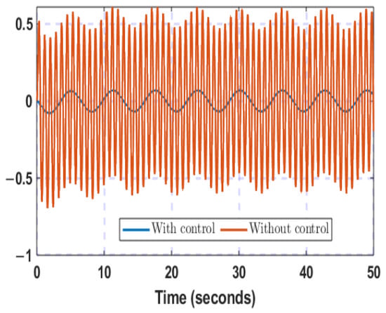
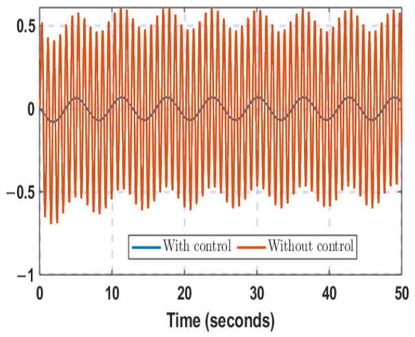
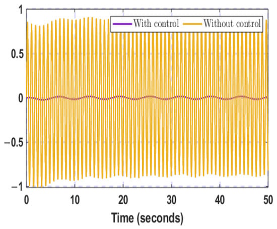
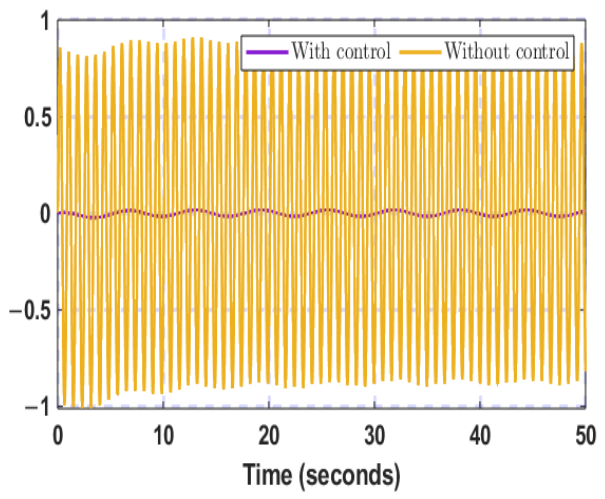
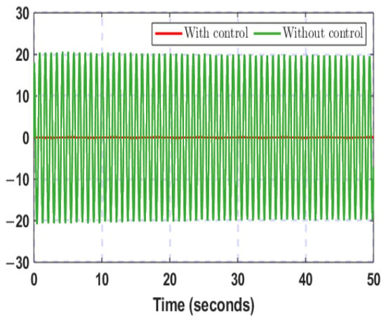
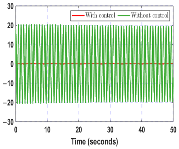
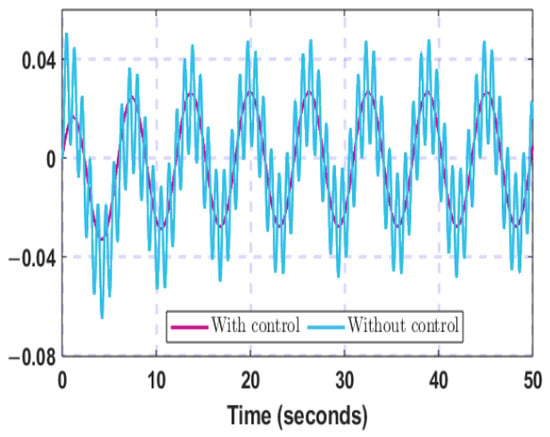
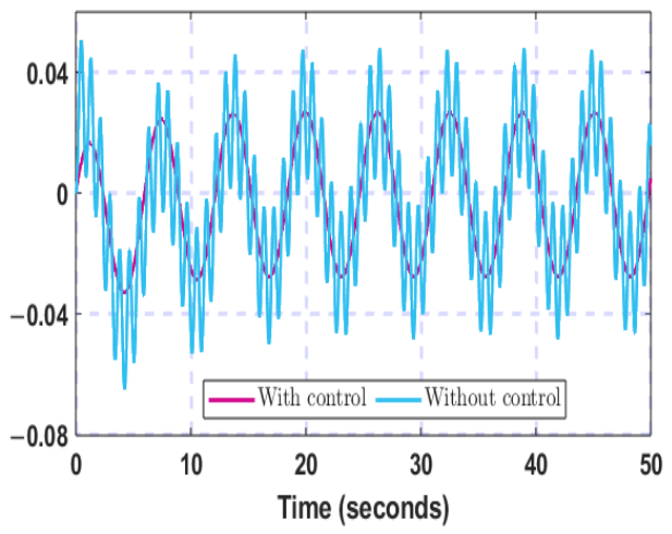
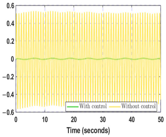
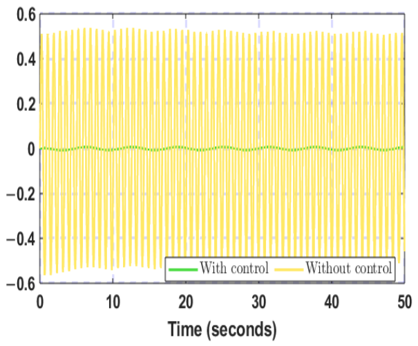
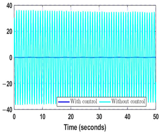
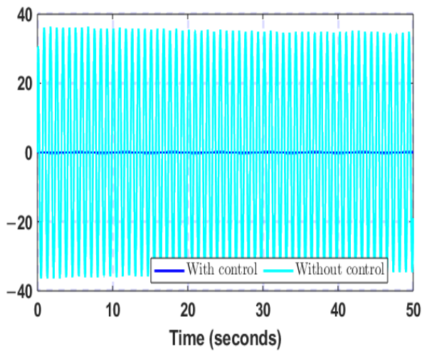
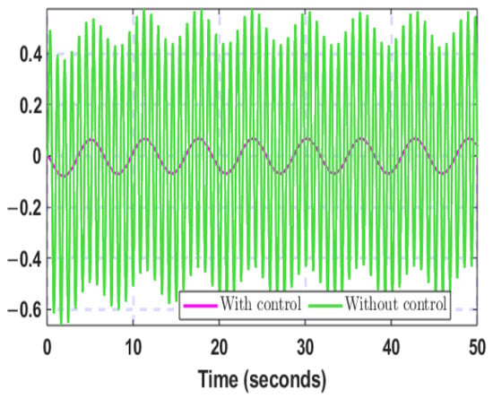
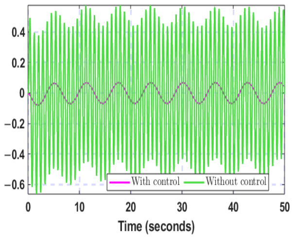
In this scenario, the nominal attack probabilities, attack-function bounds, disturbance settings, and gains specified above are used throughout. The controlled and uncontrolled responses are compared under the same nominal disturbance setting. Subsequently, by selecting the disturbance signals as $\mu \left(t\right)=\left[\begin{array}{c}0.1\sin \left(t\right)\\ 0.1\cos \left(t\right)\end{array}\right]$, the controlled and uncontrolled trajectories are compared in Figure 2, Figure 3, Figure 4, Figure 5, Figure 6, Figure 7 and Figure 8. These figures show the frequency, diesel-generator power, governor-valve position, wind-generator frequency and power, pitch-actuator output, and battery power under the same nominal scenario. The controlled trajectories exhibit smaller oscillations than the uncontrolled trajectories. The maximum absolute frequency deviation in run j is $\Delta f_{\max }^{\left(j\right)}={\max }_{0\le t\le \mathsf{T}}\left|{\eta }_1^{\left(j\right)}\left(t\right)\right|$, $j=1,2,\dots ,100$. Its average over 100 Monte Carlo runs is $0.0945$.

Figure 2. Time history of system frequency.

Figure 3. Time history of active power of the diesel generator.

Figure 4. Time profile of governor valve.

Figure 5. Time profile of frequency of wind generation.

Figure 6. Time history of active power of wind generation.

Figure 7. Time history of hydraulic pitch actuator output.

Figure 8. Response of the active power of the battery.

4.3. Observer and Disturbance-Estimation Performance

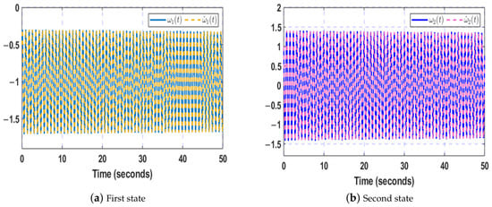
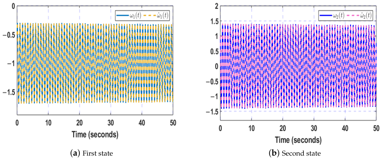
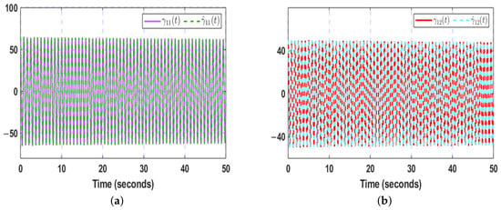
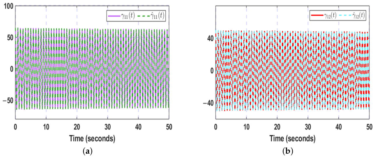
Under the nominal hybrid-attack and disturbance setting, Figure 9 shows the state-estimation error, while Figure 10 and Figure 11 show the performance of the output-reliant DO. Figure 10 compares the two exogenous-system states with their observer estimates. Figure 11 compares the corresponding matched-disturbance components with their reconstructed values. These plots assess estimation behavior separately from the frequency-regulation response.

Figure 9. Progression of state-estimation error $\parallel \tilde{\eta }\left(t\right)\parallel$.

Figure 10. Evolution of the exogenous system’s state and its corresponding DO state.

Figure 11. Evolution of matched disturbances and their estimates (a) First trajectory; (b) Second trajectory.

4.4. Finite-Time Bound and Control Effort

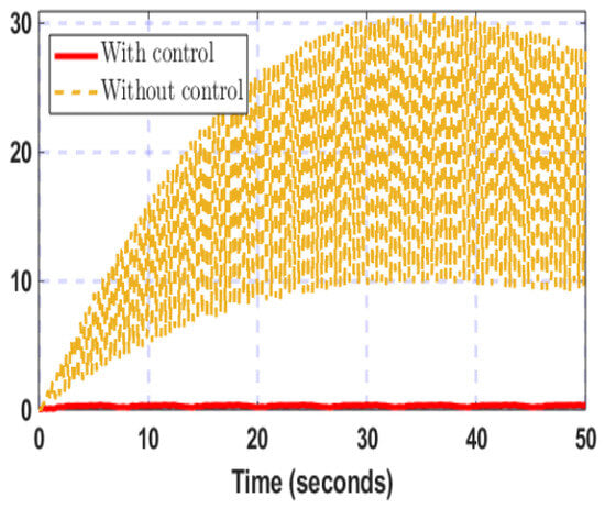
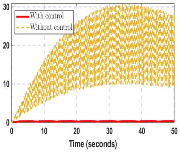
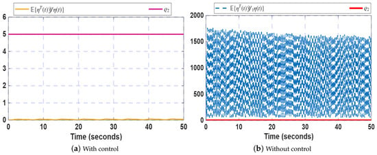
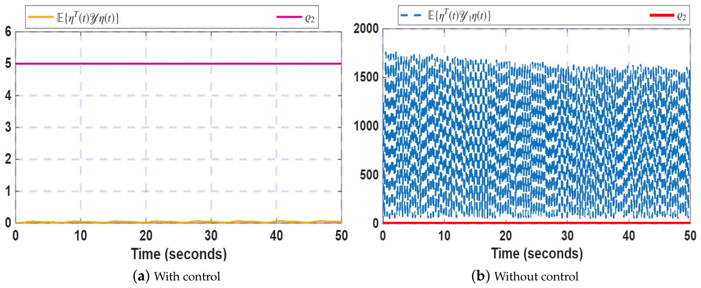
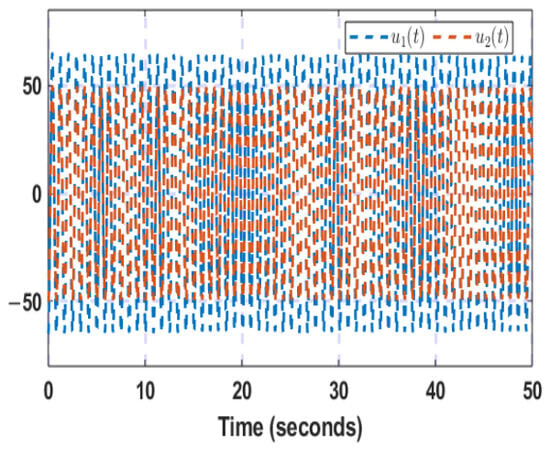
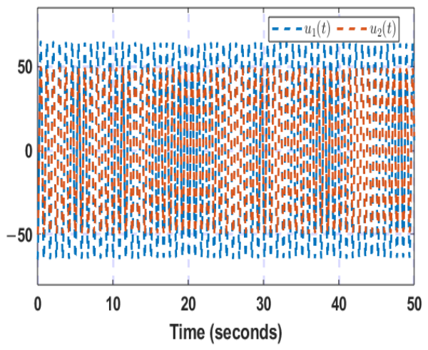
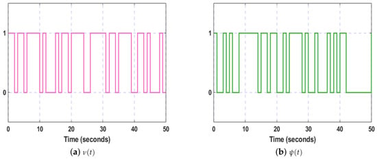
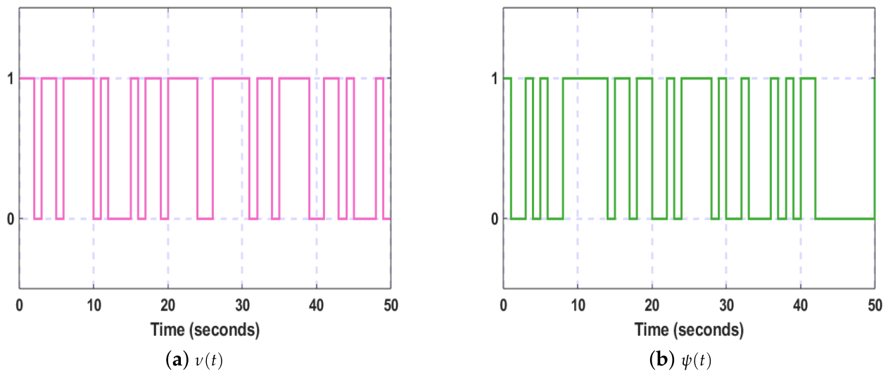
For the nominal setting with $\mathsf{T}=10$ and ${\varrho }_2=5$, Figure 12 compares the weighted state trajectory with the prescribed finite-time bound for the same parameters mentioned previously. The controlled trajectory remains below the bound over $[0,\mathsf{T}]$, whereas the uncontrolled trajectory exceeds it. Furthermore, Figure 13 displays the control-input trajectories. In addition, the control effort required by the developed ARLFC is quantified using the root-mean-square (RMS) value $u_{\mathrm{RMS}}^{\left(j\right)}=\sqrt{{\displaystyle \frac{1}{\mathsf{T}}}{\int }_0^{\mathsf{T}}{u}_j^T\left(t\right)u_j\left(t\right)dt},j=1,2,\dots ,100,$ where j denotes the Monte Carlo run. The average RMS control effort over 100 independent runs is calculated as ${\overline{u}}_{\mathrm{RMS}}={\displaystyle \frac{1}{100}}{\sum }_{j=1}^{100}{u}_{\mathrm{RMS}}^{\left(j\right)}.$ The resulting average control effort is ${\overline{u}}_{\mathrm{RMS}}=58.2125$. This result quantifies the control action required by the developed ARLFC under the considered disturbances and hybrid cyber attacks. Furthermore, the portrayal of Bernoulli variables are provided in Figure 14.

Figure 12. Time profile of ${\eta }^T\left(t\right)\mathcal{Y}\eta \left(t\right)$.

Figure 13. Time history of control trajectories.

Figure 14. Evolution of Bernoulli variables.

4.5. Monte Carlo Estimation-Error Study

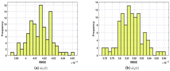
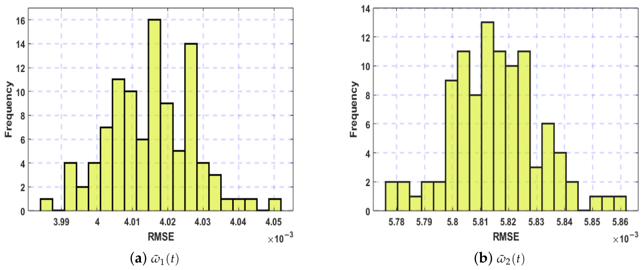
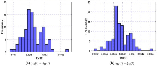
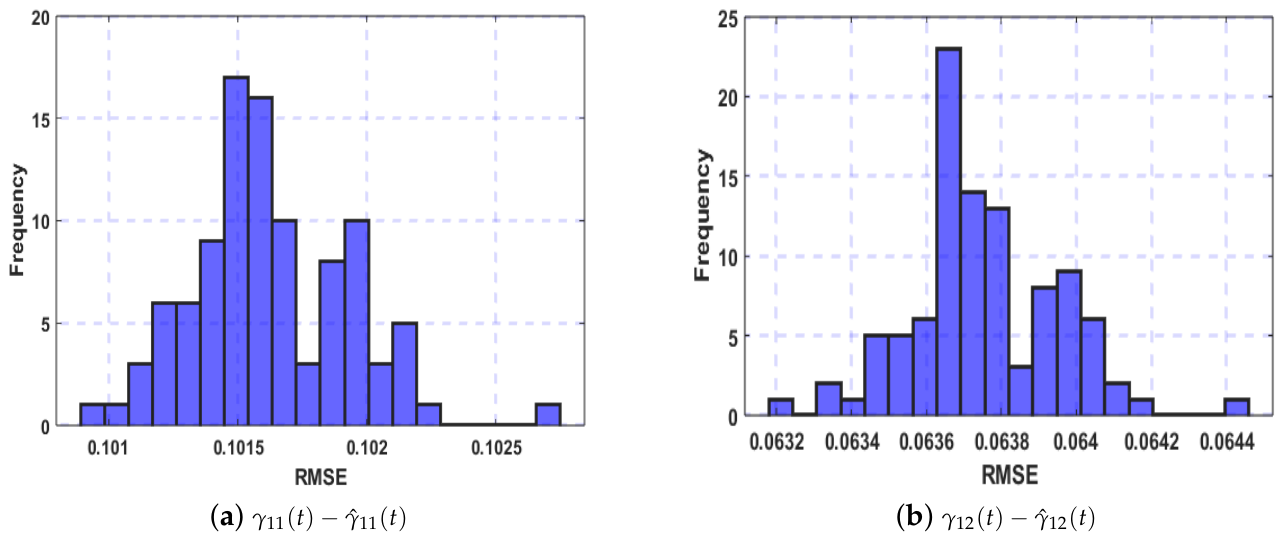
To account for stochastic hybrid-attack realizations, the nominal observer and controller configuration is evaluated over 100 independent runs. The same precomputed observer and controller gain matrices, plant parameters, disturbance settings, and attack probabilities are used in every run; only the stochastic attack realizations vary. Figure 15 and Figure 16 display the exogenous-state and matched-disturbance estimation errors, respectively, and Table 3 summarizes their root-mean-square errors (RMSE) and standard deviations. Across all 100 trials, the RMSE values remain small with a reasonably low standard deviation, demonstrating the robustness and consistency of the developed framework.

Figure 15. RMSE values of exogenous system’s state and its corresponding DO state for 100 runs.

Figure 16. RMSE values of disturbance and its estimation for 100 runs.

Table 3. Statistical performance of estimated parameters.

Performance Index	${\mathit{\gamma }}_{11}\left(\mathit{t}\right)-{\widehat{\mathit{\gamma }}}_{11}\left(\mathit{t}\right)$	${\mathit{\gamma }}_{12}\left(\mathit{t}\right)-{\widehat{\mathit{\gamma }}}_{12}\left(\mathit{t}\right)$	${\tilde{\mathit{\omega }}}_1\left(\mathit{t}\right)$	${\tilde{\mathit{\omega }}}_2\left(\mathit{t}\right)$
RMSE	0.101625	0.063750	0.004015	0.005815
Standard deviation	0.000302	0.000198	0.000012	0.000016

4.6. Controller and Observer Comparisons

Four control configurations are compared under the same nominal disturbance and hybrid-attack conditions over 100 independent Monte Carlo trials. The developed PIO-based ARLFC is the nominal proposed scheme, incorporating the disturbance observer and the proportional–integral state observer. Conventional control uses gains obtained from linear matrix inequality conditions that do not account for cyber attacks. During the Simulink evaluation, however, the same hybrid-attack signals are applied to this controller as to the other configurations. In state-feedback-based ARLFC, the disturbance observer is retained, but the actual system state is used for feedback instead of a state estimate; hence, no proportional–integral state observer is required. In Luenberger-observer-based ARLFC, the disturbance observer is retained, while the proportional–integral observer is replaced with a conventional Luenberger observer, so the integral correction structure is absent. Each configuration uses its corresponding precomputed gains, and the same disturbance and attack realizations are used for the comparisons. Table 4 reports the resulting mean output RMS values for 100 simulation runs. The developed scheme has the lowest reported average output RMS ($0.030753$), compared with $0.184518$, $0.094571$, and $0.057149$, respectively. This comparison evaluates closed-loop regulation across controller architectures.

Table 4. RMS value of output trajectory for 100 runs.

Control Method	RMS
Developed PIO-based ARLFC	0.030753
Conventional control	0.184518
State-feedback-based ARLFC	0.094571
Luenberger-observer-based ARLFC	0.057149

Subsequently, Table 5 isolates the state-observer comparison under identical disturbance and hybrid-attack realizations over 100 trials. The PIO gives an average state-estimation-error RMS of $0.198436$, whereas the conventional Luenberger observer gives $0.541892$. This result supports the role of the integral correction term in the considered scenario.

Table 5. RMS value of state-estimation error $\parallel \tilde{\eta }\left(t\right)\parallel$ for 100 runs.

Method	RMS
PIO	0.198436
Luenberger observer	0.541892

4.7. Isolated Disturbance Scenarios

In this part, the nominal hybrid-attack setting and controller are retained while the matched and mismatched disturbances are applied separately and then together. Table 6 reports output RMS values of $0.014527$ for the mismatched disturbance alone, $0.030142$ for the matched disturbance alone, and $0.030753$ for both disturbances. The combined case has the highest RMS, while all three cases remain bounded in the reported simulations.

Table 6. RMS value of output trajectory under different disturbance scenarios for 100 runs.

Scenario	RMS
Mismatched disturbance only	0.014527
Matched disturbance only	0.030142
Combined disturbances	0.030753

4.8. Isolated Attack Scenarios

Here, the nominal disturbance setting and controller are retained while replay and false-data-injection attacks are considered separately and then together. Table 7 gives output RMS values of $0.029516$ for replay only, $0.024893$ for false-data-injection only, and $0.030753$ for the hybrid case. The combined attack setting produces the largest RMS among these three scenarios.

Table 7. RMS value of output trajectory under different attack scenarios for 100 runs.

Scenario	RMS
Replay attack only	0.029516
False-data-injection attack only	0.024893
Hybrid attacks	0.030753

4.9. False-Data-Injection Occurrence Probability

In the first attack-sensitivity study, only the false-data-injection occurrence probability $\overline{\nu }$ is varied; the replay probability, attack-function bounds, disturbances, and observer–controller gains remain at their nominal settings. Table 8 reports the RMS of $\parallel \eta \left(t\right)\parallel$ for $\overline{\nu }=0.1,0.3,0.5,0.7,0.9$. The RMS increases from $0.542871$ to $0.595245$, indicating gradual performance degradation as false-data-injection attacks occur more frequently in the tested setting. The attack-function magnitudes remain unchanged in this study; only the probability of false-data-injection occurrence is varied.

Table 8. RMS value of state trajectory $\parallel \eta \left(t\right)\parallel$ under different attack probabilities $\overline{\nu }$.

$\overline{\mathit{\nu }}$	0.1	0.3	0.5	0.7	0.9
RMS	0.542871	0.552469	0.589142	0.590456	0.595245

4.10. False-Data-Injection Intensity

In the second attack-sensitivity study, the attack-function bounds $[{\mathcal{J}}_1,{\mathcal{J}}_2]$ are varied, while the attack probabilities and disturbance settings remain at their nominal values. For each bound pair, the linear matrix inequality conditions are solved again, and the corresponding observer and controller gains are used in the simulation. Table 9 reports state-trajectory RMS values of $0.426387$, $0.589142$, and $0.678412$ for the three settings. The increasing RMS indicates a larger state response as the attack-function bounds increase in the tested cases.

Table 9. RMS value of state trajectory $\parallel \eta \left(t\right)\parallel$ under different attack intensities.

$[{\mathcal{J}}_1,{\mathcal{J}}_2]$	[0.8, 0.9]	[1.7, 1.3]	[2.5, 2.7]
RMS	0.426387	0.589142	0.678412

4.11. Dissipativity-Parameter Sensitivity

With the nominal disturbance and hybrid-attack setting retained, Table 10 compares three selections of ${\mathcal{F}}_1$, ${\mathcal{F}}_2$, ${\mathcal{F}}_3$, and $\epsilon$. Their output RMS values are $0.031245$, $0.030753$, and $0.031983$, respectively; the nominal Set 2 gives the lowest value among these tested selections. This study varies the dissipativity parameters rather than the attack process.

Table 10. Sensitivity analysis of the dissipativity parameters.

Parameter Set	${\mathcal{F}}_1$	${\mathcal{F}}_2$	${\mathcal{F}}_3$	$\mathit{\epsilon }$	Output RMS
Set 1	$-0.3I$	$\left[\begin{array}{ccc}0.7& 0.7& 0.7\end{array}\right]$	$2.7I$	$0.14$	0.031245
Set 2	$-0.2I$	$\left[\begin{array}{ccc}0.5& 0.5& 0.5\end{array}\right]$	$2.5I$	$0.12$	0.030753
Set 3	$-0.4I$	$\left[\begin{array}{ccc}0.9& 0.9& 0.9\end{array}\right]$	$2.9I$	$0.16$	0.031983

4.12. Finite-Time-Bound Feasibility Sensitivity

In a separate feasibility study, the prescribed bound ${\varrho }_2$ is varied while the maximum admissible dissipativity margin ${\epsilon }_{\max }$ is evaluated. Table 11 shows that ${\epsilon }_{\max }$ changes from $2.4991$ to $2.4997$ as ${\varrho }_2$ increases from 5 to 11.

Table 11. ${\epsilon }_{\max }$ for different finite-time bounds.

${\mathit{\varrho }}_2$	5	7	9	11
${\epsilon }_{\max }$	$2.4991$	$2.4994$	$2.4996$	$2.4997$

Thus, based on the analysis presented above, we conclude that the HWDPS (3) is stabilized by the designed DO-driven ARLFC law (11), such that the DO functions properly and the system performs smoothly despite multiple disturbances and hybrid cyber attacks.

5. Conclusions

An ARLFC strategy for HWDPSs has been presented to address the challenges posed by hybrid cyber attacks and multiple disturbances within an FTB framework. The combined use of an output-reliant DO and a PIO enables reliable estimation of disturbances and system states using measured outputs. By explicitly incorporating multimodal false-data-injection and replay attacks in the controller channel, the developed ARLFC scheme maintains satisfactory frequency regulation even under adversarial signal manipulation. The FTB conditions derived in the linear matrix inequality framework offer a systematic and implementable design methodology. Simulation studies confirm that the developed approach effectively suppresses disturbance effects and mitigates attack-induced performance degradation, thereby improving the operational resilience of HWDPSs. Some limitations remain in the present framework, including the effects of measurement noise, communication delays, packet losses, sampling frequency, and actuator saturation. These limitations will be addressed in future work by extending the observer–controller framework and incorporating reinforcement-learning-based mechanisms to improve its adaptability and resilience against unknown or time-varying disturbances and cyber attacks.

References

- Almeida, R.G.D.; Lopes, J.P. Participation of doubly fed induction wind generators in system frequency regulation. IEEE Trans. Power Syst. 2017, 22, 944–950. [Google Scholar]
- Serban, I.; Marinescu, C. Aggregate load-frequency control of a wind-hydro autonomous microgrid. Renew. Energy 2011, 36, 3345–3354. [Google Scholar] [CrossRef] [Scilit]
- Mohamed, T.H.; Morel, J.; Bevrani, H.; Hiyama, T. Model predictive based load frequency control design concerning wind turbines. Int. J. Electr. Power Energy Syst. 2012, 43, 859–867. [Google Scholar] [CrossRef] [Scilit]
- Fu, L.; Cui, S.; Liu, H. Event-triggered control for ts fuzzy multi-area cyber-physical power system under hybrid attacks. J. Frankl. Inst. 2025, 363, 108366. [Google Scholar] [CrossRef] [Scilit]
- Shen, Z.; Chen, G.; Huang, T. Event-based H∞ load frequency control for fuzzy Markov-jump IPS with wind power under hybrid attacks. J. Frankl. Inst. 2024, 361, 106909. [Google Scholar] [CrossRef] [Scilit]
- Mi, Y.; Fu, Y.; Li, D.; Wang, C.; Loh, P.C.; Wang, P. The sliding mode load frequency control for hybrid power system based on disturbance observer. Int. J. Electr. Power Energy Syst. 2016, 74, 446–452. [Google Scholar] [CrossRef] [Scilit]
- Dahiya, P.; Mukhija, P.; Saxena, A.R. Design of sampled data and event-triggered load frequency controller for isolated hybrid power system. Int. J. Electr. Power Energy Syst. 2018, 100, 331–349. [Google Scholar] [CrossRef] [Scilit]
- Abdelrahim, M.; Almakhles, D.J. Synthesis of state/output feedback event-triggered controllers for load frequency regulation in hybrid wind-diesel power systems. Appl. Sci. 2023, 13, 9652. [Google Scholar] [CrossRef] [Scilit]
- Pandey, S.K.; Mohanty, S.R.; Kishor, N.; Catalão, J.P. Frequency regulation in hybrid power systems using particle swarm optimization and linear matrix inequalities based robust controller design. Int. J. Electr. Power Energy Syst. 2014, 63, 887–900. [Google Scholar] [CrossRef] [Scilit]
- Xu, T.; Zhu, C.; Qi, W.; Cao, J.; Cheng, J.; Shi, K.; Pan, G. Finite-time composite control for fuzzy delayed semi-Markovian jump systems with multiple disturbances and uncertainty. Int. J. Adapt. Control Signal Process. 2023, 37, 1738–1761. [Google Scholar] [CrossRef] [Scilit]
- Zhou, Y.; She, J.; Wang, F.; Iwasaki, M. Disturbance rejection for stewart platform based on integration of equivalent-input-disturbance and sliding-mode control methods. IEEE/ASME Trans. Mechatron. 2023, 28, 2364–2374. [Google Scholar] [CrossRef] [Scilit]
- Kaviarasan, B.; Kwon, O.M.; Park, M.J.; Sakthivel, R. Reduced-order filtering for semi-Markovian jump systems against randomly occurring false data injection attacks. Appl. Math. Comput. 2023, 444, 127832. [Google Scholar] [CrossRef] [Scilit]
- Zhao, H.; Wei, X.; Zhang, H.; Karimi, H.R. Nonlinear disturbance observer-based control for a class of discrete-time stochastic systems with multiple heterogenous disturbances. Trans. Inst. Meas. Control 2020, 42, 180–187. [Google Scholar] [CrossRef] [Scilit]
- Wang, X.; Li, S.; Lam, J. Distributed active anti-disturbance output consensus algorithms for higher-order multi-agent systems with mismatched disturbances. Automatica 2016, 74, 30–37. [Google Scholar] [CrossRef] [Scilit]
- Wei, Y.; Liu, G.P.; Zong, G.; Shen, H. Composite anti-disturbance control for uncertain Markovian jump systems with actuator saturation based disturbance observer and adaptive neural network. J. Frankl. Inst. 2019, 356, 6926–6945. [Google Scholar] [CrossRef] [Scilit]
- Li, Y.; Chen, M.; Shi, P.; Li, T. Stochastic anti-disturbance flight control for helicopter systems with switching disturbances under Markovian parameters. IEEE Trans. Aerosp. Electron. Syst. 2022, 59, 2933–2946. [Google Scholar] [CrossRef] [Scilit]
- Qin, Y.; Wang, J.; Chen, X.; Shi, K.; Shen, H. Anti-disturbance synchronization of fuzzy genetic regulatory networks with reaction-diffusion. J. Frankl. Inst. 2022, 359, 3733–3748. [Google Scholar] [CrossRef] [Scilit]
- Shen, M.; Zhang, H.; Nguang, S.K.; Ahn, C.K. H∞ output anti-disturbance control of stochastic Markov jump systems with multiple disturbances. IEEE Trans. Syst. Man Cybern. Syst. 2020, 51, 7633–7643. [Google Scholar] [CrossRef] [Scilit]
- Huang, T.; Shao, Y.; Li, L.; Liu, Y.; Shen, M. Guaranteed cost event-triggered H∞ control of uncertain linear system via output disturbance observer. Appl. Math. Comput. 2024, 473, 128652. [Google Scholar] [CrossRef] [Scilit]
- Ponnarasi, L.; Pankajavalli, P.B.; Lim, Y.; Sakthivel, R. Distributed state estimation-based resilient controller design for IoT-enabled microgrids under deception attacks. Appl. Energy 2024, 374, 123997. [Google Scholar] [CrossRef] [Scilit]
- Yan, S.; Yang, X.; Park, J.H. Outlier-removal memory-event-triggered proportional-integral state estimation for wind turbine systems under multimodal deception attacks. IEEE Trans. Autom. Sci. Eng. 2025, 22, 17790–17800. [Google Scholar] [CrossRef] [Scilit]
- Selvaraj, P.; Kwon, O.M.; Lee, S.H.; Sakthivel, R. Sampled radial basis function neural network adaptive observer-based platooning control for autonomous vehicles with cyber-attacks. IEEE Trans. Intell. Transp. Syst. 2025, 26, 23113–23124. [Google Scholar] [CrossRef] [Scilit]
- Xue, M.; Lam, J.; Yan, H.; Kwok, K.W. Asynchronous control for interval type-2 fuzzy nonhomogeneous Markov jump systems against successive DoS attacks. IEEE Trans. Cybern. 2024, 55, 172–183. [Google Scholar] [CrossRef] [Scilit]
- Qishui, Q.; Han, S.; Shi, K.; Zhong, S.; Cai, X.; Kwon, O.M. Distributed secure sampled-data control for distributed generators and energy storage systems in microgrids under abnormal deception attacks. Appl. Energy 2022, 326, 119948. [Google Scholar] [CrossRef] [Scilit]
- Yang, M.; Zhai, J. Predictor-based decentralized event-triggered secure control for nonlinear cyber-physical systems under replay attacks and time delay. IEEE Trans. Control Netw. Syst. 2023, 11, 150–160. [Google Scholar] [CrossRef] [Scilit]
- Zhang, L.; Shen, Z.; Niu, B.; Zhao, N. Dynamic-event-based reachable set synthesis for nonlinear delayed hidden semi-Markov jump systems under multiple cyber-attacks. IEEE Trans. Syst. Man Cybern. Syst. 2024, 55, 587–598. [Google Scholar] [CrossRef] [Scilit]
- Wang, X.; Park, J.H.; Wang, J.; Zhang, D. Neural network-based adaptive LFC approach for multi-area power systems vulnerable to hybrid attacks. IEEE Trans. Smart Grid 2026, 17, 2480–2489. [Google Scholar] [CrossRef] [Scilit]
- Zhang, G.; Shen, H.; Wang, J.; Cao, J.; Rutkowski, L. Resilient H∞ output feedback control for hidden semi-Markov jump systems subject to hybrid cyber attacks. IEEE Internet Things J. 2026, 13, 13072–13081. [Google Scholar] [CrossRef] [Scilit]
- Li, H.; Zhan, X.; Yang, Q.; Cheng, L.; Wu, B. Dynamic event-triggered control for networked control systems under hybrid cyber-attacks. Asian J. Control 2026, 28, 737–749. [Google Scholar] [CrossRef] [Scilit]
- Zhang, D.W.; Liu, G.P. Secure tracking control of cyber-physical systems against hybrid attacks via FAS terminal sliding-mode predictive control. IEEE Trans. Cybern. 2025, 55, 5177–5188. [Google Scholar] [CrossRef] [Scilit]
- Liu, J.; Gu, Y.; Zha, L.; Liu, Y.; Cao, J. Event-triggered H∞ load frequency control for multiarea power systems under hybrid cyber attacks. IEEE Trans. Syst. Man Cybern. Syst. 2019, 49, 1665–1678. [Google Scholar] [CrossRef] [Scilit]
- Luo, W.; Chen, H.; Zong, G.; Zhao, X. Event-triggered neural asynchronous control of nonhomogeneous Markov jump power systems with hybrid cyberattacks and unknown states. IEEE Trans. Power Syst. 2025, 40, 3874–3886. [Google Scholar] [CrossRef] [Scilit]
- Huang, F.; Pan, Y.; Lu, Q. Observer-based event-triggered security control for nonlinear networked control systems with cyber attacks. Int. J. Robust Nonlinear Control 2024, 34, 2691–2710. [Google Scholar] [CrossRef] [Scilit]
- Tahoun, A.H.; Arafa, M. Secure control design for nonlinear cyber-physical systems under DoS, replay, and deception cyber-attacks with multiple transmission channels. ISA Trans. 2022, 128, 294–308. [Google Scholar] [CrossRef] [Scilit]
- Kchaou, M.; Tajudeen, M.H.M.; Ali, M.S.; Perumal, R.; Priya, B.; Thakur, G.K. Annular finite-time stability for IT2 fuzzy networked switched system via non-fragile AETS under multiple attacks: Application to tank reactor chemical process model. Expert Syst. Appl. 2024, 255, 124552. [Google Scholar] [CrossRef] [Scilit]
- Liu, J.; Yang, M.; Xie, X.; Peng, C.; Yan, H. Finite-time H∞ filtering for state-dependent uncertain systems with event-triggered mechanism and multiple attacks. IEEE Trans. Circuits Syst. I Regul. Pap. 2019, 67, 1021–1034. [Google Scholar] [CrossRef] [Scilit]
- VakilKandi, S.J.; Bayat, F.; Jalilvand, A.; Bartoszewicz, A. Cyber-physical systems under hybrid cyber-attacks: Resilient event-triggered H∞ control approach. ISA Trans. 2025, 163, 51–64. [Google Scholar] [CrossRef] [Scilit]
- Dou, Z.; Ding, L.; Yan, S. Dynamic integral-event-triggered control of photovoltaic microgrids with multimodal deception attacks. Symmetry 2025, 17, 838. [Google Scholar] [CrossRef] [Scilit]
- Elakkiya, V.; Satheesh, T.; Kwon, O.M.; Dharsini, C.D.; Sakthivel, R. Design of security aware ESO-based tracking control for singularly perturbed hyperbolic PDE systems under multimodal injection attacks. Chaos Solitons Fractals 2026, 209, 118504. [Google Scholar] [CrossRef] [Scilit]
- Lin, L.; Lam, J.; Ching, W.K.; Qiu, Q.; Sun, L.; Min, B. Finite-time stabilizers for large-scale stochastic Boolean networks. IEEE Trans. Cybern. 2025, 55, 2098–2109. [Google Scholar] [CrossRef] [Scilit]
- Wang, S.; Sun, C.; Chen, Q.; He, H. Composite learning fixed-time control for nonlinear servo systems with state constraints and unknown dynamics. IEEE Trans. Syst. Man Cybern. Syst. 2025, 55, 2332–2342. [Google Scholar] [CrossRef] [Scilit]
- Liu, C.; Zhao, K.; Li, J.; Yang, C. Fuzzy adaptive predefined time control with global prescribed performance for robotic manipulator under unknown disturbance. IEEE Trans. Syst. Man Cybern. Syst. 2025, 55, 3397–3410. [Google Scholar] [CrossRef] [Scilit]
- Kharrat, M.; Mercorelli, P. Neural network-based adaptive finite-time control for pure-feedback stochastic nonlinear systems with full state constraints, actuator faults, and backlash-like hysteresis. Mathematics 2025, 14, 30. [Google Scholar] [CrossRef] [Scilit]
- Qi, W.; Zhang, C.; Zong, G.; Su, S.F.; Chadli, M. Finite-time event-triggered stabilization for discrete-time fuzzy Markov jump singularly perturbed systems. IEEE Trans. Cybern. 2023, 53, 4511–4520. [Google Scholar] [CrossRef] [Scilit]
- Liu, Y.; Xia, J.; Wang, J.; Shen, H. Finite-time stability for interval type-2 fuzzy nonlinear systems via an observer-based sliding mode control. J. Syst. Sci. Complex. 2022, 35, 2223–2247. [Google Scholar] [CrossRef] [Scilit]
- Park, P.; Ko, J.W.; Jeong, C. Reciprocally convex approach to stability of systems with time-varying delays. Automatica 2011, 47, 235–238. [Google Scholar] [CrossRef] [Scilit]
Disclaimer/Publisher’s Note: The statements, opinions and data contained in all publications are solely those of the individual author(s) and contributor(s) and not of MDPI and/or the editor(s). MDPI and/or the editor(s) disclaim responsibility for any injury to people or property resulting from any ideas, methods, instructions or products referred to in the content. |
© 2026 by the authors. Licensee MDPI, Basel, Switzerland. This article is an open access article distributed under the terms and conditions of the Creative Commons Attribution (CC BY) license.