


Abstract
Variational methods and deep learning represent two distinct paradigms that have each shaped the development of modern image processing. Variational formulations are grounded in carefully designed energy functionals and partial differential equations (PDEs) that encode prior knowledge about image structure; they offer interpretability, theoretical guarantees, and strong performance. Deep learning, by contrast, learns image priors implicitly from data through highly expressive parametric models and has achieved impressive improvements across a wide range of tasks. Over roughly the past decade, a growing body of work has sought to integrate the two paradigms, combining the mathematical rigor of variational models with the representational power of deep networks. This article provides a task-oriented review of this integration. We survey the principal mathematical frameworks—total variation (TV) and its generalisations, the Mumford–Shah functional, Euler’s elastica, level set methods, and nonlinear diffusion PDEs—and describe how each has been coupled with deep architectures. We then organise the literature by tasks, covering image denoising, segmentation, reconstruction, super-resolution, inpainting, and deblurring. For each task, we survey major learning paradigms and representative deep learning integration frameworks—centred on variational loss formulation, algorithm unrolling, PDE-driven architectures, plug-and-play priors, deep image prior, and score-based generative modelling—highlighting the synergy between mathematically rigorous variational principles and empirical model performance. We further establish theoretical links: residual networks to ordinary differential equations, and score-based diffusion models to stochastic PDEs. Standard benchmarks and metrics are summarised, followed by open challenges such as cross-domain generalisation, robustness, interpretability, hallucination control, and data-efficient learning. Finally, conclusions are drawn based on the available evidence, and the maturity of each research direction is explicitly discussed. This review differs from existing surveys in three respects. It classifies methods by the locus at which the variational and the learned component are coupled—the training objective, the network architecture, or the energy minimised at inference—rather than by task or by assumption on the forward operator. It applies that single classification uniformly across six tasks, including segmentation and inpainting, which carry no explicit forward operator and therefore fall outside the scope of existing surveys of learned inverse problems. Moreover, it uses the resulting coverage map, audited entry by entry against a formal membership criterion, to distinguish combinations that have been realised from those that remain unexplored, those the taxonomy excludes, and those connected only loosely.
MSC:
68U10
1. Introduction
1.1. Motivation
Image processing is related to applied mathematics, signal processing and computer vision. Classical approaches formalise a task—denoising, segmentation, reconstruction, and the like—as the minimisation of an energy functional that balances data fidelity against regularisation terms expressing prior beliefs about the solution. The seminal Rudin–Osher–Fatemi (ROF) total variation denoising model [1], the Mumford–Shah functional for segmentation and piecewise smooth approximation [2], the Chan–Vese active contour model [3], the anisotropic diffusion framework of Perona and Malik [4], and the level set machinery of Osher and Sethian [5] are widely regarded as foundational milestones. These variational and partial differential equation (PDE)-based models have several advantages: they are mostly convex or have a distinct non-convex structure; they ensure the convergence of the corresponding algorithms; they require fewer data to be adjusted; and their solutions can be explained by geometric or physical priors.
Deep learning, in the form of convolutional neural networks (CNNs), generative adversarial networks (GANs), transformers, and, more recently, diffusion models, has produced a complementary set of advances. Architectures such as the U-Net [6] have become standard tools for prediction tasks, while residual networks [7] and vision transformers [8] have extended the reach of data-driven image models. In many tasks of practical interest, deep models trained on large datasets have delivered quality improvements over purely hand-crafted variational baselines, especially when training data are plentiful and the test distribution is reasonably close to the training distribution.
Neither approach is always the most suitable. The variational methods might not work well when the hand-made priors are unable to properly reflect the complexity of natural or medical images, and their parameters must be modified according to the specific task. On the other hand, the deep networks may fail in dealing with distribution changes, usually do not possess clear structures and generally require a lot of training data. Therefore, there has been an increasing research on combining these two techniques, either by embedding classical variational or PDE structures into the deep architectures or using learning networks to replace some steps of the variational procedures. Several authors believe that such a combination will lead to models which can effectively use the data, are physically reasonable and empirically competitive [9].
1.2. Complementary Strengths
Any summary of how the two paradigms complement each other is necessarily schematic, but several contrasts stand out. With variational and PDE-based methods, the regularity of the solution can be controlled explicitly, be it piecewise constancy, piecewise smoothness or bounded curvature. Physical forward models, such as the Radon transform in computed tomography or the Fourier sampling operator in magnetic resonance imaging, fit naturally into these formulations, and the existence and uniqueness of their solutions can be analysed rigorously. Deep networks, for their part, excel at learning complex, high-dimensional priors directly from data and, once trained, perform inference at low computational cost. When a variational formulation provides the overall structure and a neural network learns selected components, the resulting hybrid has been shown to inherit useful properties of both approaches [10,11].
Integration does not, however, invariably produce genuine improvements. The evidence in the literature is mixed. On the positive side, deep networks unrolled from proximal algorithms have been reported to achieve competitive reconstruction accuracy together with improved interpretability [12,13]. Other studies are more cautious and draw attention to how sensitive such methods are to hyperparameter settings or to the choice of the underlying variational model. A careful review should therefore regard integration not as a universal solution but as a design space whose trade-offs need to be assessed case by case.
1.3. Scope and Organisation
This review focuses on image processing tasks in which a variational or PDE-based formulation has been combined with a deep neural component. We cover six core tasks—denoising, segmentation, reconstruction (inverse problems), super-resolution, inpainting, and deblurring—giving each the same structural treatment, in the sense made precise below. Within each task section, we will discuss the classical variational baseline, purely deep approaches, and integrated approaches; we then consider how different learning paradigms—supervised, unsupervised, self-supervised, semi-supervised, and contrastive—have been applied.
Literature was selected as follows. We searched Scopus, IEEE Xplore, and arXiv, combining the name of each variational framework (total variation, Mumford–Shah, Euler’s elastica, level set methods, nonlinear/anisotropic diffusion) with each of the six task names and with each learning-paradigm term, and supplemented the result by backward and forward citation chasing from the foundational papers [1,2,3,4,5] and from the surveys [10,13,14,15,16]. A work was included if it couples a variational or PDE-based component with a learned component in one of the three structural senses defined in Section 3, or if it is a foundational or state-of-the-art reference required as a baseline for such a coupling. A work was excluded if the variational model appears only as a cited baseline without structural coupling; if the contribution is a purely sequential pipeline in which a learned stage merely post-processes a variational one, or the converse (Section 3); if the target task lies outside the six considered here, such as registration, classification, or detection; or if it is available only as an unreviewed preprint, unless the peer-reviewed literature has subsequently built on it, as is the case for several diffusion-model papers. The resulting reference list is therefore representative rather than exhaustive: the aim was to cover every framework–strategy–task combination that has established literature, not every paper within each combination.
Equal weight across the six tasks is structural rather than bibliometric. Each of Section 4, Section 5, Section 6, Section 7, Section 8 and Section 9 follows the same template—the classical variational baseline, purely learned approaches, then integration under Strategies A, B, and C in turn—so that the same questions are put to every task and the sections are of comparable length. Coverage is deliberately not equal in the number of works cited, which would misrepresent the field: reconstruction and denoising have attracted substantially more integrated work than inpainting or deblurring, and we state this imbalance explicitly rather than concealing it. Where a strategy has no established instance for a task, we say so rather than filling the slot.
The remainder of the paper is organised as follows. Section 2 reviews the mathematical foundations of variational and PDE-based image processing and summarises the deep learning primitives most relevant to our scope. A taxonomy of integration strategies is introduced in Section 3, after which Section 4, Section 5, Section 6, Section 7, Section 8 and Section 9 treat, in turn, denoising, segmentation, reconstruction, super-resolution, inpainting, and deblurring. Commonly used datasets, metrics, and benchmarks are collected in Section 10. Section 11 takes learning paradigms as a cross-cutting theme and also discusses the theoretical links between network architectures and differential equations. Open challenges and possible future directions are identified in Section 12; Section 13 consolidates the task-level comparison, and Section 14 concludes the paper.
1.4. Relation to Prior Surveys
Parts of this territory have been covered by several recent surveys and tutorials. Monga, Li and Eldar [13], for example, give an authoritative account of algorithm unrolling, but they restrict themselves to that one integration strategy and to inverse-problem reconstruction. Loss-side integration (e.g., Mumford–Shah and boundary losses), implicit-prior methods (plug-and-play, regularisation by denoising (RED) and the deep image prior) and the more recent diffusion-based posterior samplers therefore lie outside their scope. Ongie et al. [10] review deep learning for inverse problems with considerable attention to its theoretical foundations. Their focus, too, is on reconstruction, and prediction problems such as segmentation, deblurring and inpainting are not covered. Thorough surveys of deep learning for denoising and for segmentation are available from Tian et al. [16] and Minaee et al. [14], respectively, while Siddique et al. [15] concentrate on U-Net variants for medical imaging. Each of these, however, addresses a single task and engages only to a limited extent with the variational tradition in which the corresponding task formulations originated. A growing literature on score-based generative priors covers the diffusion thread, yet it usually frames these priors as an outgrowth of generative modelling. It rarely presents them as a development of variational regularisation and gradient-flow PDEs, with which they are mathematically continuous.
The present review argues that these threads are instances of a small number of integration strategies applied to a similarly small set of variational frameworks across six imaging tasks. The strategies are the variational regulariser as a training loss, algorithm unrolling, and the implicit prior in iterative inference. The frameworks are total variation, Mumford–Shah, Euler’s elastica, level set methods and nonlinear diffusion. Viewed in this way, it becomes clear which framework–paradigm intersections are mature, which are still at an early stage, and which are conspicuously absent. The same perspective also exposes the structural factors behind divergent lines of progress. In image reconstruction, of which low-dose CT is the paradigmatic case, advances have come mainly from one integration strategy. Progress in segmentation, of both natural and medical images, has instead been driven by different ones. Beyond mapping the field, the taxonomy helps to identify what integration actually improves. A central question is whether two properties survive the coupling of the variational and learned components in training and inference, or are even strengthened by it: the convergence guarantees inherited from the variational side and the empirical performance contributed by the learned side. Section 3.4 takes up this question directly. The rest of the review is organised to bring these structural patterns to the fore rather than to catalogue methods task by task in isolation.
Specifically, this review makes the following contributions:
(i) a unified taxonomy built on three strategies (the variational regulariser used as a training loss, algorithm unrolling, and the implicit prior within iterative inference), which places plug-and-play, RED, variational losses, PDE-inspired architectures, the deep image prior, bilevel optimisation and diffusion priors in one common framework; (ii) a synthesis of work on six tasks (denoising, segmentation, reconstruction, super-resolution, inpainting and deblurring), organised according to this taxonomy; (iii) a cross-cutting analysis of the ways in which supervised, unsupervised, self-supervised, semi-supervised and contrastive learning paradigms interact with each variational framework; (iv) an audited coverage map, which lists, for every framework–paradigm intersection, the methods that couple the two structurally and, where there are none, records whether the combination is unexplored in the surveyed literature, excluded by the taxonomy, or only loosely connected; (v) an explicit account of the open challenges: theoretical convergence guarantees under learned operators, scaling to volumetric and dynamic data, standardised evaluation of interpretability and uncertainty, cross-protocol generalisation in clinical imaging, and integration with vision foundation models. A timeline of representative methods, grouped by integration strategy, is given in Figure 1.
Figure 1.
Timeline of representative methods. The two panels use different time scales. Panel (a) covers the pre-deep-learning era, in which the foundational variational and PDE-based models were established: level sets [5], Mumford–Shah [2], Perona–Malik [4], ROF/TV [1], geodesic active contours [17], Chan–Vese [3], elastica inpainting [18], Split Bregman [19], LISTA [20] and Chambolle–Pock [21]. Panel (b) covers the deep-learning era, in which the four hybrid families discussed in Section 3 emerged—algorithm unrolling (ADMM-Net [22], TNRD [12], ISTA-Net [23], LEARN [24], VarNet [11], and the unrolling survey [13]), plug-and-play and implicit priors (PnP priors [25], PnP-ADMM [26], RED [27], Deep Image Prior [28], DeepRED [29], TV+DIP [30], Double-DIP [31], DPIR [32] and deep variational priors [33,34]), geometry-aware variational losses (deep level sets [35], topology-aware loss [36], boundary loss [37], active-contour-mimicking network [38] and Mumford–Shah loss [39]), and score-based solvers for inverse problems (DDPM [40], Score-SDE [41], DDRM [42], RePaint [43], DPS [44] and reverse-diffusion MRI [45]). Splitting the axis keeps the dense post-2015 period legible, since roughly three quarters of the methods surveyed here fall within its final decade. Method family is encoded by marker shape as well as by colour, so the grouping remains readable in greyscale.
Two of these surveys propose classifications that partly overlap with the one adopted here, and it is worth stating precisely where the difference lies. Monga et al. [13] classify methods within algorithm unrolling—by which optimiser is transcribed, which parameters are freed, and how the resulting network is trained; their partition is therefore internal to what we call Strategy B, and by construction, it says nothing about loss-side integration or about priors invoked at inference. Ongie et al. [10] classify by the epistemic status of the forward operator whether A is known, partially known, or unknown and whether the learned component is trained with it. That criterion is powerful for inverse problems but is undefined wherever no forward operator exists, which excludes segmentation outright and admits inpainting only through a degenerate masking operator. Neither classification is wrong; both are indexed by domain, whereas the question asked here is structural.
We classify instead by a single question: at which point of the pipeline does the learned component enter the variational object—in the objective that trains the network (Strategy A), in the composition structure of the network itself (Strategy B), or in the energy that is actually minimised at test time (Strategy C)? This criterion is operator-free, hence, applicable across all six tasks surveyed here; it is checkable rather than descriptive—the membership test is stated formally at the beginning of Section 3—and, because the three loci are logically independent, it makes combinations enumerable rather than anecdotal. Table 1 maps the earlier classifications onto this one and records what each leaves uncovered. Table 2 then applies the taxonomy to the surveyed literature, recording for each framework–paradigm intersection which methods are structurally coupled and which couplings remain unexplored.
Table 1.
Relation between this taxonomy and the classifications adopted by earlier surveys. Each earlier partition is indexed by a different variable, and each is silent about regions of the literature that the present criterion reaches.
Table 2.
Structurally coupled methods by variational framework (rows) and learning paradigm (columns). An entry appears only if the cited work couples the framework with a learned component in the sense of the membership criterion of Section 3; the letter in parentheses gives the strategy. Marks in empty cells distinguish combinations for which no coupled work was found (○), combinations whose only candidates the taxonomy excludes (×), and combinations with only a loose or indirect connection (∼); see the note below the table.
Compared with the previous version, every entry has been checked against the criterion of Section 3. Purely learned methods that had been listed because they are historically related to a framework or serve as its baselines—DnCNN [53], RED-CNN [54], WGAN-VGG [55], Noise2Noise [56], Noise2Void [57], Noise2Self [58], Mean Teacher [59], UA-MT [60], SimCLR [61], MoCo [62], and the contrastive scheme of [63]—have been removed, as have DIP [28], DeepRED [29], and Double-DIP [31], which belong to Strategy C but couple to none of the five frameworks; the classical, non-learned models [17,18,52]; LISTA [20], whose ℓ1 synthesis prior is not a total-variation model; and SSDU [64], a self-supervised unrolled network whose learned regulariser is not one of the five frameworks. Other entries have been moved to the framework or paradigm their authors actually use.
Three observations follow, and we state them with the caution the audit requires. First, the contrastive column is empty: none of the works we surveyed couples a contrastive objective structurally to any of the five frameworks. An admissible coupling would need a contrastive objective that itself encodes the variational prior, for instance, positive pairs generated by a scale-space semigroup, and we are not aware of such work. Second, semi-supervised coupling is represented only by the Mumford–Shah loss [39], which its authors demonstrate in supervised, semi-supervised, and unsupervised settings; generic semi-supervised schemes are purely learned. Third, Euler’s elastica has no structurally coupled learned method in the surveyed literature; its cells record either classical solvers that the taxonomy excludes or loose analogies, and the numerical explanation offered in Section 3.5 is a hypothesis rather than a finding. A cell marked ○ therefore records an absence in the literature we surveyed, not a demonstrated research opportunity: a gap may equally reflect a mismatch between prior and paradigm that no future work will overcome.
2. Mathematical Foundations
2.1. Variational Formulation of Image Processing
In a generic variational formulation, an image u defined over a domain Ω ⊂ ℝ2 (or ℝ3 for volumetric data) is recovered as the minimiser of an energy functional of the form
where D is a data-fidelity term that measures the discrepancy between the estimate u and the observed data f (for example, f may be a noisy observation, a set of projection measurements, or a masked image), R is a regularisation term that encodes prior knowledge about admissible images, and λ > 0 is a regularisation parameter. The precise form of D is typically dictated by the forward model and the assumed noise statistics. For Gaussian noise, D(u, f) = ½ ‖Au − f ‖2, where A is the forward operator. For Poisson noise, a Kullback–Leibler-type data term is common.
E(u) = D(u, f) + λ R(u),
The geometric and statistical character of the solution is determined by the choice of R. Quadratic penalties of Tikhonov type, among the earliest regularisers, smooth the image uniformly; they are simple and convex, yet their tendency to blur edges is what prompted the search for edge-preserving alternatives. The classical variational and PDE frameworks reviewed in this section are listed in Table 3 together with their analytical properties and typical applications, and comprehensive treatments can be found in the monographs [65,66,67].
Table 3.
Classical variational and PDE frameworks underlying the methods reviewed in this survey.
2.2. Classical Regularisers and PDE-Based Models
2.2.1. Total Variation
Of the edge-preserving regularisers, the total variation (TV) seminorm, which Rudin, Osher and Fatemi [1] first applied to image processing, is arguably the most influential. In its continuous isotropic form, TV(u) = ∫Ω|∇u|dx; replacing the Euclidean norm of the gradient by the ℓ1 norm yields anisotropic variants. Minimising TV favours piecewise constant solutions while retaining sharp discontinuities. Because the functional is convex, it can be optimised efficiently, for instance by splitting schemes such as Split Bregman [19] or by primal-dual algorithms [21]; Chambolle’s projection algorithm [68] was an early efficient solver. A known drawback is that TV introduces staircase artefacts where the intensity varies smoothly. This has led to variants such as TV-ℓ1 [69], total generalised variation (TGV) [70], which penalises higher-order derivatives in a balanced way, and non-local TV [71], which extends the penalty to non-local neighbourhoods. Weighted and anisotropic formulations of TV offer a means of incorporating further geometric priors.
2.2.2. Mumford–Shah Functional
The Mumford–Shah (MS) functional [2] provides a piecewise smooth model. Given an image f, one seeks a function u (piecewise smooth) and a discontinuity set K such that
where H1(K) is the one-dimensional Hausdorff measure (length) of the edge set K. Minimising this functional is difficult because of the free discontinuity term; the Ambrosio–Tortorelli approximation replaces K with a phase-field function and admits Γ-convergence guarantees. The Chan–Vese model [3] can be viewed as a piecewise-constant specialisation of the MS energy, replacing the smooth region term with region-mean approximations and representing the edge set implicitly via a level set function. The MS framework remains a touchstone for segmentation and smoothing, and its combination with deep learning has received increasing attention, for example, through learned piecewise-smooth losses [39] (see Section 5.3).
E(u, K) = ∫Ω\K |∇u|2 dx + ν H1(K) + μ ∫Ω (u − f)2 dx,
2.2.3. Euler’s Elastica and Curvature-Based Regularisation
Euler’s elastica energy penalises both the length and the integrated squared curvature of the level curves of an image:
where κ denotes the curvature of a level line and a, b ≥ 0 weight the two contributions. The curvature term favours smooth continuation and has theoretical appeal for inpainting disoccluded regions, where connectivity of level lines is a natural prior, as argued by Masnou and Morel [72] and by Shen, Kang, and Chan [18]. Owing to its non-convexity and the presence of higher-order derivatives, elastica minimisation is numerically challenging; augmented Lagrangian [52] and operator-splitting schemes have been proposed. Deep variants that learn curvature-aware regularisation from data are an area of active investigation.
Eela(u) = ∫Ω (a + b κ2) |∇u| dx,
2.2.4. Level Set Methods
The level set method of Osher and Sethian [5] represents a moving interface Γ ⊂ Ω implicitly, as the zero level set of a continuous function φ: Ω → ℝ. A Hamilton-Jacobi equation for φ then governs how the interface evolves, and topological changes such as splitting and merging are handled by this formulation without any special treatment. Level sets underlie edge-based segmentation models, of which geodesic active contours [17] are the best known, as well as region-based ones such as Chan–Vese [3]. They can also be combined with deep learning in several ways: through level-set losses, through learned speed functions, or by training networks to predict signed distance maps [35].
2.2.5. Nonlinear and Anisotropic Diffusion PDEs
Perona and Malik [4] proposed the model ∂u/∂t = div(g(|∇u|)∇u), in which the diffusivity g weakens smoothing in the vicinity of edges. The equation is forward-backward parabolic and hence ill-posed [73]. Existence and uniqueness can be recovered by smoothing the gradient before the diffusivity is evaluated [74,75] and by replacing the scalar diffusivity with a diffusion tensor, a change that additionally yields scale-space properties and admits efficient splitting schemes [65,76,77]. Fourth-order variants avoid staircasing because they favour piecewise-planar, not piecewise-constant, solutions [78]. In reaction-diffusion equations, an extra term pushes the solution towards features of interest. One discretised step of such an equation is structurally identical to a feed-forward layer, which means that its coefficients can be learned [79]; this is exactly what TNRD [12] exploits (Section 3.2, Section 3.4 and Section 11.6).
2.3. Deep Learning Primitives
The deep architectures that recur below are assumed familiar and are recalled only by name: convolutional networks with residual connections [7]; the U-Net encoder–decoder with long skip connections [6], the de facto standard for dense prediction; generative adversarial networks [80]; transformers and their image variants [8,81], with hybrid designs such as the Swin Transformer restoring locality through shifted windows [82]; and score-based and denoising diffusion models [40,41], which reverse a forward noising process and are surveyed for inverse problems in [83]. What matters for this review is not their internal detail but where each can be attached to a variational model, which is the subject of Section 3.
2.4. Optimisation Tools for Variational Models and Deep Networks
Convex analysis and non-smooth optimisation provide the foundations of variational image processing. Proximal operators generalise projection; for several important regularisers, including TV [68] and sparsity-inducing norms, they admit closed-form expressions. ADMM [84,85], primal–dual methods [21], forward–backward splitting and similar splitting schemes decouple the data-fidelity term from the regulariser, with convergence rates that follow from monotone-operator theory.
Deep learning, by contrast, optimises a different objective with a different set of tools. The quantity minimised is an empirical risk over the training samples, which is non-convex in the network weights. Minimisation proceeds by stochastic first-order methods, namely SGD with momentum and adaptive variants such as Adam, with gradients computed by backpropagation; regularity is imposed through weight decay, normalisation layers and learning-rate schedules. The difference between the two approaches is systematic. On the variational side, a deterministic and typically convex problem is solved for each image, and optimality can be certified. On the learned side, a stochastic, non-convex problem is solved once over an entire dataset, and performance is validated empirically.
The two toolboxes meet where a splitting scheme becomes a network: in unrolled architectures, each layer is a proximal or gradient step, so a proximal operator must be differentiable for backpropagation to pass through it, and the outer stochastic optimiser tunes parameters of an inner deterministic solver. These algorithms therefore serve not only as solvers but also as templates for the unrolled networks of Section 3.1, and the interaction between the two optimisation regimes is what Section 3.4 examines.
3. Integration Strategies: A Taxonomy
A wide variety of mechanisms have been proposed to couple variational or PDE-based ideas with deep learning. Although no single classification is canonical, the taxonomy adopted here, adapted from previous surveys [10,13], organises the principal design patterns by where the coupling occurs: in the training objective (Strategy A), in the network architecture (Strategy B), or in the prior invoked during iterative inference (Strategy C). The three loci can be separated precisely. Write an integrated system as a triple (, Fθ, ): the training objective, the parameterised architecture, and the inference map that produces from the observation y. Let E(x) = D(x, y) + λR(x) denote the variational energy from which the classical component derives. Strategy A: R enters only, and is a single evaluation, = Fθ(y). Removing R after training changes nothing about inference; the variational model has acted purely as a training-time inductive bias. (The bilevel form is the dual case: R is retained at inference, and selects its parameters.) Strategy B: Fθ = TK ∘ … ∘ T1, where each TK is a parameterised instance of one iteration of a solver for E, so that the layer index is the iteration index. The test is the existence of a bijection between layers and solver steps; where it holds only genealogically (Section 3.2.2), we say so. Strategy C: is itself an iterative procedure whose limit satisfies a stationarity or fixed-point condition containing a learned operator, 0 ∈ ∂D(, y) + λ ∂Rθ() or = Ψθ(). Equivalently: the learned component is required at test time and is invoked more than once.
The criterion is exhaustive over the literature surveyed here and yields three corollaries that the classifications of [10,13] cannot express. First, it applies unchanged to tasks with no forward operator, which is what allows segmentation (Section 5) and inpainting (Section 8) to be placed on the same axis as reconstruction. Second, since the three loci are logically independent, hybrids are enumerable: A+B, A+C, and B+C all occur (Section 6.2), and A+B+C does not, an absence we return to in Section 3.5. Third, and most consequentially, failure modes turn out to cluster by locus rather than by task: the same expressiveness–certification tension recurs in every Strategy C system regardless of whether the task is denoising or MRI reconstruction (Section 3.4 and Section 3.5).
Figure 2 gives a schematic comparison of the three strategies, and Figure 3 refines Strategy C in more detail. Many successful systems in practice draw on more than one strategy, so the assignment that follows reflects where integration primarily takes place in each family of methods. Purely sequential pipelines, such as analytic reconstruction followed by learned post-processing, compose the two paradigms rather than coupling them structurally: they share neither the objective, nor the architecture, nor the inference loop. Such pipelines are therefore discussed under the relevant tasks and not within this taxonomy, although Section 3.2.2 considers residual denoisers that can be interpreted as diffusion steps. Composition is orthogonal to the taxonomy, since a learned or variational post-processing stage can be appended to any pipeline in either direction. A system is classified according to the innermost locus of structural coupling and is regarded as a sequential baseline only when composition is the sole relationship between the two paradigms.
Figure 2.
Three integration strategies for combining variational methods with deep learning. Strategy A inserts a variational regulariser into the training loss of an otherwise data-driven network; representative methods are the Mumford–Shah loss [39], boundary loss [37], active-contour CNN [48], bilevel fields-of-experts [86] and deep level sets [35]. Strategy B unrolls each iteration of a model-based optimiser into a learnable network stage; representative methods are LISTA [20], ADMM-Net [22], ISTA-Net [23], VarNet for MRI [11] and LEARN for CT [24]. Strategy C invokes a data-derived prior—a denoiser, score model, or untrained generator—inside an iterative inference loop; representative methods are PnP-ADMM [26], RED [27], Deep Image Prior [28], DeepRED and Double-DIP [29,31], and diffusion-based solvers such as DPS and DDRM [42,44]. Each strategy is discussed in the corresponding subsection of Section 3.
Figure 3.
Three structurally distinct ways of injecting a learned prior into reconstruction. PnP substitutes an off-the-shelf denoiser D<sub>σ</sub> into the proximal slot of ADMM/HQS, with no explicit regulariser [25,32]. RED treats the denoiser as defining an explicit regulariser 𝓡<sub>RED</sub>(x) = ½x<sup>T</sup>(x − D(x)) whose gradient is added to the data-fidelity gradient [27,29]. DIP parametrises the image itself as the output of an untrained CNN G<sub>θ</sub>(z), optimising θ to fit a single measurement y; the network architecture acts as the prior [28,31]. Author–year labels in the figure correspond to these references.
3.1. Strategy A: Objective-Level Coupling
In the first strategy, the two paradigms are coupled through the objective function, while the network architecture and the inference procedure remain unchanged. This strategy takes two complementary, and in fact dual, forms. In one, a variational term is added to the loss used to train a network. In the other, a learned component is embedded in a variational energy, and the parameters of that energy are tuned through an outer learning problem.
3.1.1. Variational Regularisation as a Learning Loss
The most direct construction embeds variational terms into the training loss of a deep network. Mumford–Shah-type losses regularise segmentation networks towards piecewise-constant regions and, through the total-variation term they contain, towards short boundaries [38,39]; curvature-based losses in the spirit of Euler’s elastica have been proposed far less often, for reasons discussed in Section 3.5. Works that combine a deep network with an explicit variational energy by optimising the network parameters per image [33,47] do not belong here: the energy is minimised at inference, so they are instances of Strategy C (Section 3.3.2). Geodesic and level-set-inspired losses have also appeared in segmentation [37,48]. Such losses are typically easy to implement as differentiable penalties and impose inductive biases without structural changes to the backbone.
3.1.2. Bilevel Optimisation
The converse construction places the variational model, rather than the network, at the centre. Bilevel optimisation casts the selection of variational hyperparameters—regularisation weights, or even entire regularisers—as an upper-level learning problem whose lower level is the variational reconstruction. This allows task-specific tuning of variational models in a principled way [86,87]. Although often more computationally demanding than standard training, bilevel approaches yield models with the interpretability of the underlying variational formulation and have been used, for example, to learn filter banks in fields-of-experts models. Together with variational losses, they illustrate the two directions in which objectives can be shared: the former lends variational structure to network training; the latter lends learning capacity to variational models.
3.1.3. Optimisation of Strategy A
The two forms of Strategy A lead to different optimisation problems. In the loss-based form, the variational term is simply added to an otherwise standard training objective, L(θ) = L_task(uθ) + λR(uθ), which is minimised end-to-end by stochastic gradient methods. The only requirement is that R be differentiable along the computation graph. TV is therefore replaced by a smooth Charbonnier or Huber surrogate, and curvature terms, which involve higher-order spatial derivatives, are computed on the network output with finite-difference stencils. Optimisation in this setting is no more difficult than ordinary training; the main practical difficulty is choosing λ so that the regulariser is properly balanced against the task loss.
The bilevel form is considerably harder, because the parameters being trained appear inside an argmin. At the upper level, a task loss is minimised over hyperparameters θ, and the corresponding reconstruction u*(θ) is itself the solution of the lower-level variational problem. There are two ways to compute the hypergradient. Implicit differentiation applies the implicit function theorem to the optimality conditions of the lower-level problem. It is exact, but it requires the lower-level problem to be solved to high accuracy and its Hessian to be inverted, or at least the associated linear system to be solved iteratively. Unrolled differentiation, on the other hand, backpropagates through a fixed number of lower-level iterations, which is cheaper but only approximate. If the truncated iterations are additionally given free parameters of their own, this approach reduces to the algorithm unrolling of Section 3.2, so Strategy B can be understood as a relaxation of bilevel learning [12,86]. The choice between the two has consequences for the guarantees discussed in Section 3.4. Implicit differentiation keeps the lower-level model exactly intact, whereas unrolling gives up this fidelity in exchange for scalability.
3.2. Strategy B: Coupling in the Architecture
In the second strategy, variational or PDE structure is built into the network itself, and the inductive bias is therefore carried by the architecture rather than by the loss. Each layer corresponds to an iteration of a model-based solver or to a time step of a differential equation.
3.2.1. Algorithm Unrolling
Algorithm unrolling (also called algorithm unfolding or deep unfolding) turns a fixed number of iterations of a classical iterative solver into a trainable neural network. Every layer stands for one iteration of the original algorithm, and some or all of its parameters, such as step sizes, proximal operators or filter coefficients, are learned from data. LISTA [20], derived by unrolling the iterative shrinkage-thresholding algorithm (ISTA) for sparse coding, was the pioneering example. In image processing, trainable nonlinear reaction diffusion (TNRD) [12] unrolls a nonlinear reaction–diffusion PDE and has been reported to improve denoising and deblocking performance. For compressed-sensing MRI, ADMM-Net [22] and ISTA-Net [23] unroll ADMM and ISTA, respectively, and variational networks have been designed for MRI reconstruction [11]. What makes unrolling attractive is that the network keeps the interpretability and convergence intuition of the underlying algorithm while gaining representational flexibility. This close coupling to the original solver comes at a price, however: the forward model is fixed in the architecture, so the network cannot easily be adapted to a new measurement operator without substantial redesign. Recent unrolled reconstruction methods have continued along these lines; examples from 2024 include an iterative residual optimisation network for limited-angle tomography [88] and a sparse–low-rank unrolling network for spectral CT [89]. A self-supervised unrolled scheme based on regularisation by denoising has also been proposed, which dispenses with fully sampled reference data [90].
3.2.2. PDE-Inspired Architectures
Whereas unrolling reproduces one particular solver step by step, a looser form of architectural coupling borrows differential equations as design motifs. A residual block in a ResNet [7] may be read as a forward Euler discretisation of an ODE dx/dt = f(x, θ(t)) [91,92]; this reading motivated neural ODEs [93] as well as families of stable architectures [91]. When a network is derived from anisotropic diffusion or reaction–diffusion PDEs, each layer update corresponds to an explicit PDE time step [12]. Multi-scale architectures, pyramid networks and nonlocal modules often draw their motivation from classical multiscale analysis and nonlocal filtering, such as nonlocal means [94] and its sparse-representation successors, of which BM3D [95] is the most prominent.
The same architectural perspective helps to locate residual denoising networks that are otherwise trained purely as post-processors. DnCNN [53] uses residual learning: it predicts the noise component and subtracts it, so its update u−f(u) can be interpreted as a single explicit step of a learned diffusion. In fact, one-stage TNRD can be recovered as a special case of this architecture [53]. Encoder-decoder variants developed for low-dose CT, such as RED-CNN [54], inherit the same residual structure through their shortcut connections. These networks nonetheless do not satisfy the membership criterion stated at the start of this section. Their layers are not iterations of a solver for any explicit energy, and the diffusion-step interpretation is an analogy with the reaction–diffusion lineage of TNRD [12], not a structural coupling. We therefore do not assign DnCNN, RED-CNN or the adversarially trained WGAN-VGG [55] to any strategy. They appear in this review only as purely learned baselines and have been removed from Table 2 and Table 6.
3.2.3. Optimisation of Strategy B
After a solver has been unrolled into T layers, training becomes ordinary end-to-end stochastic optimisation of a T-layer network. Three features, however, set it apart from generic deep learning. First, the forward operator and its adjoint appear in every layer, so each gradient step requires T applications of both. In tomography and MRI these operations account for most of the computational cost, and unless gradient checkpointing is employed, the memory needed for backpropagation grows linearly with T. This is exactly the truncated-unrolling hypergradient of Section 3.1.3, except that the truncated iterations now carry free parameters. Second, whether parameters are tied across layers is a design decision with theoretical implications. If the weights are shared, the network can still be read as a fixed iterative algorithm, and fixed-point analysis remains applicable. If they are untied layer by layer, the result is the learned acceleration of LISTA [20,96], obtained at the cost of that interpretation. Third, backpropagation through many nearly identical iterations is subject to the same vanishing- and exploding-gradient problems that arise in recurrent networks. This is where the PDE perspective of Section 3.2.2 proves its value. Treating layers as explicit time steps imposes step-size restrictions analogous to the CFL condition, and architectures designed for stability [91,92] guarantee well-behaved forward dynamics, which in turn yield well-conditioned gradients. Finally, the unroll depth T is fixed during training and serves as a hyperparameter that balances accuracy against computational cost [11,22,23].
3.3. Strategy C: Learned Components Within Iterative Inference
The third strategy keeps a classical iterative inference procedure and introduces a component supplied by a network into the energy that is minimised at inference time. Membership in this strategy is defined by exactly this criterion: a learned component appears in the inference objective. That component may occupy either of the two slots in a variational energy. When it occupies the prior slot, the data-fidelity term remains classical, and the regulariser is provided in one of three ways. It may come from a pre-trained denoiser (PnP/RED), from the inductive bias of an untrained generator (DIP), or from a score model trained on clean data (diffusion priors). Figure 3 compares these three injection mechanisms, which are discussed in Section 3.3.1, Section 3.3.2 and Section 3.3.3. When the learned component instead occupies the data-term slot, a handcrafted regulariser is kept and the likelihood is predicted by a network (Section 3.3.4).
3.3.1. Plug-and-Play Priors and Regularisation by Denoising
Plug-and-play (PnP) priors [25] build on the observation that, in splitting algorithms such as ADMM, the step associated with the proximal operator of the regulariser is formally a Gaussian denoising problem. Replacing this step with an arbitrary denoiser, which may be a learned one, removes the need for an explicit functional form of the prior and allows a single denoiser to be reused for many inverse problems. Convergence analyses [26] have established conditions under which PnP iterations converge to a fixed point. Regularisation by denoising (RED) [27] offers an explicit variational interpretation: for a denoiser f, it defines the regulariser ρ(u) = ½ uᵀ (u − f(u)), which has certain consistency properties under suitable technical assumptions. In both frameworks, variational reconstruction is linked to learned priors; the variational structure is kept intact, while a deep network such as DnCNN [53] or DRUNet [32] supplies the denoiser.
3.3.2. Deep Image Prior
The deep image prior (DIP) [28] showed that a suitably parameterised convolutional network, optimised on nothing more than a single degraded image, already acts as an implicit prior for natural images. Here the prior stems from the architecture, not from training data. Some variants couple DIP with explicit variational regularisation, such as weighted total variation [30] or higher-order and selective segmentation energies [33,47]; others, DeepRED [29] among them, pair it with regularisation by denoising. DIP has found use where training data are limited, medical and scientific imaging included, but its results remain sensitive to the choice of stopping criterion [30].
3.3.3. Score-Based and Diffusion Priors
In score-based generative models and denoising diffusion probabilistic models [40,41], a network is trained to estimate the score (the gradient of the log-density) of a noise-perturbed data distribution. If this score serves as the prior in a Bayesian formulation of an inverse problem, the resulting posterior sampling algorithms are formally very close in structure to variational reconstruction [42,44]. Because the learned prior describes a distribution and is not tied to any particular forward model, a single pre-trained diffusion model can, in principle, serve many tasks, including nonlinear ones (see Section 6.3.2). Diffusion priors have recently been extended beyond Gaussian likelihoods to the exponential family, which covers Poisson and other noise models that commonly arise in imaging [97].
3.3.4. Learned Data Terms with Handcrafted Priors
In the converse direction, the regulariser remains handcrafted and the network is given the data term. For segmentation, the softmax probabilities of a trained CNN can serve as the region (likelihood) force in a variational energy whose prior carries explicit shape information, for example isoperimetric compactness; the functional is then minimised at inference by spatially continuous dual optimisation [34]. These systems meet the membership criterion of the strategy, since the network-predicted likelihood enters an energy that is genuinely optimised at inference. Sequential pipelines without any inference-time optimisation, on the other hand, are still compositions in the sense defined at the start of this section. Although many papers in this family describe their methods as “post-processing” or “refinement”, the label only reflects where the method sits in the pipeline; classification depends on the structural coupling alone. How deep the integration goes within the family depends on how informative the handcrafted prior is. Generic smoothness penalties lie at the shallow end, whereas explicit structural priors (isoperimetric compactness, topology, shape) impose constraints that the network would not provide by itself. Structurally, this direction is the mirror image of Section 3.3.1, Section 3.3.2 and Section 3.3.3, as the learned and classical slots of the energy are interchanged between the two families.
The assessments in Table 4 are qualitative, and for several of its criteria, a quantitative statement is available. Let N be the number of voxels, CA the cost of one application of A or of its adjoint, and Cθ the cost of one forward pass of the learned component Cθ = O(N · Σℓkℓ2 cℓ−1cℓ) for a convolutional network with kernel sizes kℓ and channel widths cℓ. For the operators considered here, CA = O(N log N) for FFT-based blur and single-coil MRI, O(NC · N log N) for N_c-coil MRI, and O(N3/2) for the two-dimensional Radon transform with O(√N) views. Let K denote the number of unrolled stages or of inference iterations. Table 5 records the resulting cost per reconstructed image.
Table 4.
Comparison of the three integration strategies of Section 3. Purely sequential pipelines (e.g., analytic reconstruction followed by a learned post-processor) sit outside this comparison: with no inference-time optimisation, they occupy the trivial corner of every column—paired supervision, no forward-model dependence, minimal interpretability, minimal cost (Section 3). Assessments are qualitative and refer to the typical member of each family; hybrids inherit properties from the strategies they combine.
Table 5.
Quantitative comparison of the three integration strategies. Costs are per reconstructed image in the notation defined above; P1–P4 are the verifiable properties that replace the ordinal interpretability grades of Table 4. Entries marked conditional hold only under the assumptions cited.
In the same table, the informal notion of interpretability is replaced by four properties, each of which can be verified for a given system, whereas an ordinal grade cannot. Under P1, the output is characterised as a minimiser or stationary point of an energy expressed in closed form. P2 holds when convergence as K → ∞ is provable and the required assumptions are recorded. P3 requires that every trainable parameter correspond to a quantity of the underlying model, for instance a step size, a regularisation weight, a filter or a diffusivity. P4 demands that the learned component remain valid for a forward operator not encountered during training.
What matters here is the order of magnitude rather than the exact constants. Consider four-fold accelerated multi-coil brain MRI at 320 × 320 with fifteen coils: a ten-stage unrolled network needs ten network evaluations and twenty operator applications for each reconstruction. Diffusion posterior sampling with 103 function evaluations costs a further two orders of magnitude, while a loss-integrated network requires just a single evaluation. In Table 4, the labels “low”, “low–moderate” and “high” summarise this 1:10:103 ratio qualitatively.
3.3.5. Optimisation of Strategy C
Strategy C distributes the optimisation over two timescales. In the offline phase, the injected component is trained independently of any specific inverse problem. The denoiser is trained with a standard denoising objective [53] and the score model by denoising score matching, while DIP needs no pretraining whatsoever [28]. In the online phase, the actual optimisation is carried out by the classical iterative loop, whose behaviour depends on how the learned component is injected. In PnP, the denoiser takes the place of a proximal operator within ADMM or forward-backward splitting. An explicit energy therefore does not exist in general, and the iteration is analysed as a fixed-point scheme in which the noise level of the denoiser and the penalty parameter serve as the tuning parameters [25,26]. RED, under the conditions given in [27], recovers an explicit objective whose gradient is u − D(u). DIP, for its part, optimises the network weights for each image with a first-order method. Early stopping then acts as the regulariser, and the iteration at which optimisation stops becomes the critical hyperparameter [28]. Diffusion priors alternate a reverse-time sampling process with data-consistency steps, so that both cost and fidelity are governed by the step schedule and the approximation used for the likelihood [42,44]. What these mechanisms share, and what distinguishes them from Strategies A and B, is a shift of computation from training to test time. Each reconstruction involves many network evaluations, and hyperparameters are tuned for each problem instead of being learned. In return, a single trained component can be amortised over arbitrary forward models. The conditions under which this test-time optimisation is provably convergent are precisely those examined in Section 3.4 [98,99].
3.4. Convergence and Performance: What Does Integration Enhance?
Each paradigm brings a different strength to the integration. From the variational side comes convergence, in the form of convex or otherwise well-structured energies, the theory of monotone operators and fixed points, and iterative schemes (gradient descent, ADMM, primal–dual splitting) whose convergence to a minimiser or saddle point can be proved under verifiable conditions. Deep learning contributes performance: learned priors far more expressive than handcrafted regularisers, and, when training data are abundant, an empirical accuracy that hand-designed models seldom reach. This raises a natural question for every hybrid scheme surveyed in Section 3.1, Section 3.2 and Section 3.3. Does integration preserve, or even enhance, convergence while improving performance, or does each side instead dilute the advantage of the other?
As far as convergence is concerned, the answer depends on where the learned component is introduced. In Strategy A, the inference machinery is left unchanged, and the classical guarantees carry over. Once a regulariser has been trained, as with bilevel-trained filter-based random fields [86,87] or learned regularisers such as NETT [100] and total deep variation [101], the resulting energy is minimised by standard solvers whose analysis is unaffected. Bilevel training influences only the quality of the learned parameters and has no effect on the convergence of the lower-level iteration. In Strategy B, unrolling truncates the iteration at a fixed depth, so asymptotic convergence gives way to trained behaviour over a finite number of steps. Remarkably, though, learning can increase the speed of convergence and not merely preserve it. LISTA attains a given accuracy in far fewer iterations than ISTA [20], an acceleration that has since been characterised rigorously as a linear convergence rate [96], and ADMM-Net and ISTA-Net inherit this acceleration for imaging operators [22,23]. In Strategy C, the guarantees hold only under certain conditions. PnP-ADMM converges to a fixed point if the plugged-in denoiser satisfies boundedness or nonexpansiveness assumptions [26], and RED has a consistent interpretation when Jacobian symmetry and local homogeneity conditions are met [27]. Provable convergence can be restored by enforcing such conditions, either through Lipschitz or spectral-norm constraints imposed while training the denoiser [99] or by parameterising the denoiser as an explicit gradient step, so that the iteration provably converges to stationary points of an underlying functional [98]. The cost is a more restricted class of networks.
On performance, integration clearly lifts hybrid models above the purely variational methods from which they derive. Unrolled networks do better than both the underlying optimisation scheme and generic black-box networks of comparable size, since the inherited algorithmic structure acts as an inductive bias that raises accuracy per parameter and per training sample [11,22,23]. Relative to purely data-driven models, the gains are of a different kind, concerning data efficiency, robustness to operator or distribution shift, and reusability. With PnP, a single pre-trained denoiser [32,53] improves results over an entire family of inverse problems without any task-specific retraining, and DIP delivers competitive restoration with no training data at all [28]. The regimes in which structure improves performance are therefore exactly those in which unconstrained deep learning is weakest: scarce data, shifting distributions and changing forward models.
These two kinds of enhancement do not, however, compound automatically; they pull against each other. The hypotheses that certify convergence, such as nonexpansiveness, contractivity and bounded Lipschitz constants, limit expressive capacity, and constrained denoisers generally give up some empirical accuracy compared with their unconstrained counterparts. Conversely, the learned priors that perform best regularly violate the assumptions of the convergence theorems currently available, so their excellent empirical behaviour is observed but not guaranteed. Existing integrated systems therefore tend to improve along one axis while preserving, or slightly weakening, the other. Where the balance should lie depends on the application. Safety-critical reconstruction calls for certified convergence even at a modest cost in performance, whereas photographic restoration can accept heuristic convergence in return for the highest possible quality.
The overall verdict is a qualified yes on both counts. Integration can enhance convergence in the practically relevant sense of speed—learned solvers reach prescribed accuracy in an order of magnitude fewer iterations—and can preserve convergence in the theoretical sense under enforceable constraints; and it reliably enhances performance relative to purely variational baselines while improving data efficiency and robustness relative to purely learned ones. What remains open is the simultaneous attainment of state-of-the-art performance and unconditional guarantees; the partial and uneven state of this theory is surveyed in [46] and taken up in Section 12.2.
3.5. Negative Results: Which Integrations Have Not Worked, and Why?
The account so far has recorded what integration achieves. A review that reported only successes would misrepresent the field: several couplings have been tried and found wanting, and their failures are informative. They are not scattered at random but cluster by the locus at which the coupling was made.
Plug-and-play with unconstrained denoisers. There is no guarantee that a splitting algorithm will converge once an arbitrary trained denoiser has been substituted into it. The iteration may cycle, and even when it does settle, the fixed point it reaches is determined by the penalty parameter and not by any prior. Convergence can be restored by constraining the denoiser, whether by bounding its Lipschitz constant, by requiring non-expansiveness [26,99] or by adopting an explicit gradient-step parameterisation [98], but this comes at a measurable cost in accuracy. Here the tension between expressiveness and certification identified in Section 3.4 appears in its most acute form.
The explicit variational reading of RED. RED was introduced with an explicit regulariser whose gradient is u—D(u) [27]. Reehorst and Schniter [102] showed that this reading requires the denoiser to have a symmetric Jacobian and to be locally homogeneous and that trained convolutional denoisers satisfy neither; the gradient interpretation therefore does not hold for the methods actually deployed, and what survives is a fixed-point reading connected to score matching. We retain RED within Strategy C on the strength of that weaker interpretation, and the statements about RED in Section 3.3.1 and Section 3.4 should be read subject to it.
Unrolling: acceleration bought with interpretability. Untying parameters across layers buys LISTA-style acceleration [20,96] at the cost of the reading of the network as a fixed iterative algorithm, and as depth grows and parameters are fully untied, an unrolled network approaches a generic network of comparable size. What unrolling contributes is an inductive bias rather than the algorithm itself, and like other inductive biases, its value diminishes as training data grow.
Structured post-processing absorbed by stronger backbones. Dense conditional random fields were standard in early semantic segmentation and were unrolled into recurrent layers by CRF-RNN [103]; DeepLabv3+ [104] removed the stage, reporting that a stronger decoder made it unnecessary, and it has largely disappeared from competitive pipelines. The same pattern appears in medical segmentation, where nnU-Net [105] shows that systematic self-configuration of a plain U-Net outperforms most architectural and loss-side embellishments, geometric losses among them. A prior that duplicates what abundant data already supply is absorbed as backbones and datasets grow.
Metric gains that are not clinical gains. Antun et al. [106] showed that deep reconstruction can become unstable under small perturbations, to the point of omitting clinically relevant detail, and Gottschling et al. [107] contend that this behaviour is generic and not merely incidental. In the 2020 fastMRI challenge [108], the organisers named AI-generated hallucination, along with the inadequacy of current metrics, as one of the main open problems. They also reported that radiologists held mixed views of the reconstructions at eightfold acceleration and on scanners outside the training distribution. The leading submission nevertheless ranked first on both SSIM and radiologist assessment, which shows that metrics and readers do not necessarily disagree. Evaluation practice is thus itself part of the failure mode, an issue revisited in Section 10.4.
Higher-order geometric priors: a numerical rather than conceptual failure. Curvature and elastica terms require second derivatives of the network output, realised by finite-difference stencils that are poorly conditioned under stochastic optimisation, and curvature is undefined on the thresholded masks that semi-supervised schemes produce. This, rather than any argument that curvature is the wrong prior, is, we suggest, the principal reason why the elastica row of Table 2 contains no structurally coupled method—the obstruction is numerical, and a phase-field relaxation on soft predictions is the obvious route around it.
These findings divide along the lines of the taxonomy rather than along task boundaries. Redundancy is the failure mode of Strategy A: a geometric prior that only duplicates what abundant labels already convey is absorbed as models grow larger. Strategy B suffers from dilution, because untied parameters and greater depth reintroduce black-box behaviour, and the interpretability that first motivated unrolling ends up being traded for accuracy. For Strategy C, the obstacle is the cost of certification: the hypotheses that make an iteration provably convergent exclude the best-performing denoisers. A fourth failure mode, which concerns evaluation practice and lies outside the taxonomy, is that distortion metrics can improve even while clinically salient structure is being fabricated or lost. In practice, then, integration justifies its added complexity precisely where data cannot substitute for structure: when annotations are scarce, when forward operators change, or when constraints such as measurement consistency are required that no amount of training data can supply. If a larger dataset and a well-configured baseline would suffice, integration is a poor investment.
4. Image Denoising
Of all imaging tasks, denoising is probably the one in which the integration of variational methods and deep learning has been explored most extensively. Denoising also acts as a component of many other restoration pipelines through PnP, RED and diffusion-based sampling. As a result, progress in denoising tends to carry over to reconstruction, super-resolution and inpainting.
4.1. Purely Learned Denoising
4.1.1. Supervised Deep Denoising
Given paired training data, supervised denoising networks learn a direct mapping from noisy to clean images. The line of work starts with DnCNN [53], which pairs residual learning with batch normalisation. FFDNet [109] followed; because it is conditioned on a noise-level map, a single model can cover a wide range of noise variances. Feature attention for real noise was introduced in RIDNet [110], while NAFNet [111] relies on a simplified backbone. Adding perceptual and adversarial terms [112] steers the outputs towards visually plausible reconstructions, and transformer backbones, SwinIR [113] and Restormer [114] for example, achieve competitive performance.
4.1.2. Unsupervised and Self-Supervised Denoising
Where clean references are unavailable, self-supervision replaces them. Noise2Noise [56] maps one noisy observation to another and recovers the clean image under zero-mean noise; Noise2Void [57] and Noise2Self [58] remove even that requirement by masking pixels and predicting them from their surroundings; Neighbor2Neighbor [115] builds training pairs by subsampling adjacent pixels; and deep image prior [28] needs only the degraded image itself. These schemes carry denoising into medical and scientific modalities where paired data cannot be acquired.
4.1.3. Contrastive and Representation-Based Denoising
Contrastive learning serves less as a denoising objective than as a way of pre-training representations for downstream restoration, typically with losses defined between clean and degraded patches or between augmentations of a noisy image. The evidence base is thinner than for the other categories here, and quantitative claims should be checked against the originating papers. Figure 4 shows the unified reconstruction pipeline.
Figure 4.
The unified reconstruction pipeline. Stages 1–3 derive the variational functional from imaging physics (Beer–Lambert for CT, k-space sampling for MRI, blur kernels for natural images) by writing the forward model y = Ax + n and the MAP estimator. Stage 4 selects the regulariser R(x) from classical options—total variation [1], Mumford–Shah [2] and Euler’s elastica [18]—or from learned priors such as PnP [25], DIP [28] and score-based models [41]; stage 5 chooses the optimisation algorithm. Variational–deep-learning hybrids enter at stage 4 (loss-side integration) or stage 5 (unrolling, implicit priors).
4.2. Strategy A: Variational Regularisation in the Denoising Objective
Strategy A is comparatively rare in denoising: variational penalties are more often attached to the per-image objective of a deep image prior than to the training loss of a denoiser. The DIP variants that add total-variation or Hessian penalties to curb overfitting [29,30] minimise that penalty at inference on a single image, and under the criterion of Section 3, they therefore belong to Strategy C; they are discussed in Section 4.4.
4.3. Strategy B: Unrolling-Based Denoising
Unrolled networks provide an explicit bridge between classical variational denoising and deep learning. TNRD [12] unrolls a nonlinear reaction–diffusion PDE into a trainable feed-forward network, with filters and influence functions learned from data; the resulting architecture has been reported to achieve strong performance with a relatively small number of stages. Subsequent works have unrolled primal–dual algorithms, forward–backward splitting, and ADMM for denoising. A conceptual advantage is that each layer corresponds to a recognisable algorithmic step, which facilitates interpretation and, in some cases, analysis of convergence. Figure 5 illustrates how the iterations of such a model-based solver are mapped onto the cascaded stages of a learnable network.
Figure 5.
From iterative optimisation to a learnable network. The left panel shows the model-based iterative formulation (proximal gradient on a variational functional with a hand-set prior); the right panel shows one stage of the unrolled network, in which the proximal step is replaced by a CNN with learnable parameters. K iterations become K cascaded stages whose parameters {(αk, θk)} are optimised jointly by backpropagation on paired training data.
4.4. Strategy C: Plug-and-Play and Implicit Priors
Within the PnP and RED frameworks, deep denoisers act as modular priors inside variational solvers. In DPIR [32], a flexible CNN denoiser trained by Zhang et al. is inserted into half-quadratic splitting, and this single system achieves competitive results across denoising, deblurring, super-resolution, and demosaicing. To curb the overfitting to which DIP is prone, DeepRED [29] combines it with a RED prior, while the ADMM scheme of [30] uses weighted total variation instead. On the theoretical side, studies of PnP convergence have identified conditions, nonexpansiveness of the denoiser among them, under which the fixed-point iterations are well behaved [26].
4.5. Denoising in Medical Imaging
Low-dose computed tomography (LDCT) denoising is a representative clinical problem. RED-CNN [54] uses a residual encoder–decoder CNN trained on paired low-dose and normal-dose slices and reports visible improvements on the Mayo Clinic data. WGAN–VGG [55] combines a Wasserstein GAN loss with a perceptual VGG loss in order to reduce the over-smoothing artefacts that are typical of ℓ2 training. Transformer-based architectures, CTformer-type designs among them, have been proposed to capture long-range dependencies within CT slices. More recently, diffusion-based denoisers have been studied, including some that rely on physics-aware noise models derived from the Beer–Lambert law. Research on such physics-informed denoising is still developing, and quantitative comparisons are highly sensitive to the dose level, the reconstruction kernel, and the patient cohort; aggregate numerical rankings should therefore be interpreted with caution.
5. Image Segmentation
The aim of segmentation is to partition an image into regions corresponding to meaningful structures. In the classical variational setting, this is done with energies that combine a data-fidelity term and geometric priors, the latter imposed either on the region boundaries or directly on the labelling field. Deep learning has transformed the field, initially with encoder–decoder networks and, more recently, with transformer-based architectures. Variational ideas now enter chiefly through loss design, architectural hybrids, and unrolling.
5.1. Classical Variational Segmentation
A canonical formulation is the Mumford–Shah functional [2], which treats boundaries as free discontinuities between smooth regions. Chan–Vese [3] restricts this model to piecewise constant approximations and evolves a level set function along the gradient flow of the associated energy. Geodesic active contours [17] instead replace the region term with an edge-dependent length penalty, so that contours move along the gradient of a Riemannian length. Such models are amenable to rich theoretical analysis, and they offer interpretable control over the geometry of the segmentation.
Among the further extensions are the piecewise smooth MS model, multiphase level set formulations for multi-region segmentation, and shape priors introduced via statistical atlases or curvature-based penalties. Euler’s elastica has also been investigated as a higher-order shape regulariser in selective segmentation, where it encourages smooth boundaries in the presence of noise or occlusion.
5.2. Purely Learned Segmentation
5.2.1. Deep Segmentation Architectures
The encoder–decoder paradigm for dense prediction was established by FCN [116] and U-Net [6]. DeepLab [117] subsequently introduced atrous convolutions and dense-CRF post-processing, and on natural-image benchmarks the lead has since passed to transformer models such as SegFormer [118] and Mask2Former [119]. With Segment Anything [120], promptable general-purpose segmentation arrived in the form of a foundation model; MedSAM [121] adapted it to medical images, and Medical SAM 2 [122] carries SAM 2 over to medical volumes by treating them as video. In medical imaging, nnU-Net [105] remains the reference point, since its self-configuring pipeline matches or outperforms more elaborate designs, while TransUNet [123] and Swin-UNet [124] offer transformer-based alternatives.
5.2.2. Semi-Supervised Segmentation
Labels for dense segmentation are costly; semi-supervised learning is therefore of high practical interest. Consistency regularisation approaches encourage predictions to be stable under perturbations of the input or the network (e.g., Mean Teacher [59]). Pseudo-labelling methods generate labels for unlabelled data and retrain; FixMatch-style schemes [125] combine weak and strong augmentations with confidence thresholding. Uncertainty-aware self-ensembling [60] has been applied to medical volumetric segmentation. These schemes are purely learned. A variational loss evaluated on the unlabelled images can supply the training signal the labels do not, as the Mumford–Shah loss does in its semi-supervised form [39], but among the works we surveyed, this is the only structurally coupled semi-supervised method.
5.2.3. Contrastive Learning for Segmentation
Segmentation encoders have been pre-trained with contrastive self-supervised representation learning, including SimCLR [61], MoCo [62], BYOL [126], SimSiam [127], and supervised contrastive learning [128], and are then usually fine-tuned under supervision. For medical image segmentation with limited annotations, Chaitanya et al. [63] proposed a contrastive scheme combining global and local features, and reported that pre-training with volumetric contrastive losses benefits downstream segmentation when labelled data are scarce. Subsequent studies have explored contrastive objectives tailored to dense prediction, such as pixel-level and region-level contrast.
5.2.4. Unsupervised and Zero-Shot Segmentation
Unsupervised segmentation draws only on the structure of the image itself and has traditionally been approached through clustering, MS-type models, and graph partitioning. Modern deep approaches include self-supervised pretext tasks, saliency-driven methods, and the generation of candidate masks with pre-trained foundation models. The deep image prior has also been adapted to segmentation. In Double-DIP [31], for instance, coupled DIP networks decompose an image into foreground and background layers without any external training data, and the inductive bias of the network architecture serves as an implicit regulariser for a data-dependent segmentation energy. Zero-shot segmentation with large models such as SAM [120] is a related and rapidly developing line of research, although these models have so far incorporated classical variational structure only to a limited extent.
5.3. Strategy A: Coupling in the Training Objective
5.3.1. Variational and Geometric Losses
A considerable body of work adds variational terms that encode geometric priors to the standard pixelwise losses (cross-entropy, Dice). TV regularisation of the segmentation masks, for instance, discourages noisy boundaries. Mumford–Shah-inspired losses, among them those built on Ambrosio–Tortorelli relaxations, favour piecewise smooth predictions with controlled discontinuities [39]. Topology-aware losses steer networks towards structurally coherent boundary geometry and thereby complement curvature-based regularisation in the spirit of Euler’s elastica; Mosinska et al. [36], for example, penalise topologically inconsistent predictions through distances between VGG features. The boundary loss [37], the Hausdorff distance loss and other boundary-aware losses aim to improve geometric fidelity.
5.3.2. Level-Set-Based Deep Segmentation
A number of studies incorporate a level set representation into a deep segmentation pipeline. The network may predict a signed distance function (SDF) or output a level set function directly, and the loss functions are derived from Chan–Vese or geodesic active contour energies [35,38]. The approach thus joins the representational flexibility of deep networks to the geometric and topological versatility of level sets, and it has been investigated for medical image segmentation as well as for natural-image tasks.
5.4. Strategy B: Unrolled and PDE-Inspired Segmentation
Segmentation has seen unrolling in several forms. CRF-RNN [103], which unrolls mean-field inference of a dense CRF into recurrent layers trained end-to-end with the backbone, is still the canonical case of an energy-minimisation scheme transcribed into a segmentation architecture. In the continuous setting, deep structured active contours learn the parameter maps of an active-contour energy and embed its minimisation in training [129], while LevelSet R-CNN differentiates through a truncated level-set optimisation within an instance-segmentation head [50]. PDE-inspired architectures, in turn, treat the propagation of masks or features as a diffusion process. In the semantic diffusion network, for instance, boundary enhancement is implemented as a learnable anisotropic diffusion step [51]. PottsMGNet, by contrast, derives the encoder–decoder architecture itself from operator splitting of a Potts segmentation model, thus providing a variational explanation for an empirically motivated design [49]. These designs pair the end-to-end trainability of deep networks with the interpretability of energy minimisation or PDE evolution.
6. Image Reconstruction (Inverse Problems)
Reconstruction of images from indirect measurements is one of the settings in which the integration of variational methods and deep learning is most visible. Recovering an image u from measurements f = A(u) + η, where A is the forward operator and η the noise, is usually an ill-posed problem, so regularisation based on image priors is indispensable. Classical methods combine a handcrafted regulariser, such as TV or a wavelet-sparsity term, with an iterative solver. Deep learning has brought data-driven priors into the reconstruction pipeline at several levels. Figure 4 sketches this pipeline, from the imaging physics and the choice of regulariser to the optimisation algorithm, and marks the points at which variational–deep-learning hybrids come into play.
6.1. Classical Reconstruction
Tikhonov and TV-regularised reconstruction, and compressed sensing with sparsifying transforms [130], are the mathematical backbone of modern tomography and accelerated MRI: under incoherent measurements and approximate sparsity, ℓ1-regularised reconstruction recovers under-sampled signals stably. ISTA, FISTA, ADMM, and primal–dual splitting [21] are the standard solvers, and they remain in clinical use where predictable behaviour is required.
6.2. Strategy A and Multi-Strategy Hybrids
For reconstruction, Strategy A appears as learned regularisers that leave the variational energy explicit at inference. The template came from bilevel parameter learning, in which TV-type weights are tuned against a task loss and the reconstruction forms the lower-level problem [87]. More recent descendants replace the handcrafted functional itself. An adversarial regulariser trains a critic network to tell desirable from undesirable images and then uses that network directly as R(u) [131]. NETT places a trained network inside a Tikhonov-type functional and establishes convergence of the resulting regularisation scheme in the classical inverse-problems sense [100], whereas total deep variation learns a multi-scale regulariser whose stability and optimality conditions can be analysed through the associated gradient flow [101]. Because inference remains the minimisation of an explicit energy, this family rests on the firmest theoretical footing of all learned reconstruction methods, which is exactly the convergence side of the trade-off examined in Section 3.4.
Many practical systems combine several strategies. A learned denoiser may act as a PnP prior inside a primal–dual loop whose regularisation weights are tuned by bilevel learning [26,87], or a score-based prior may be stabilised by an explicit TV term [44]. Such hybrids reflect the observation that no single integration strategy is adequate in every operating regime.
6.3. Strategy B: Supervised Unrolled and Physics-Embedded Reconstruction
6.3.1. MRI Reconstruction
Variational networks for MRI [11] unroll a generalised compressed-sensing gradient descent with learned filters and activation functions. They have been reported to reconstruct accelerated multi-coil data quickly, and in a reader study, the resulting image quality was judged suitable for clinical evaluation. MoDL [132] shares weights across iterations and uses a conjugate-gradient data-consistency layer; this reduces the amount of training data required, and the method is reported to generalise across several acceleration factors. ADMM-Net [22] and ISTA-Net [23] are further examples of unrolled networks for compressed-sensing reconstruction. Taken together, these methods show that the interpretability of classical iterative algorithms can be retained while the representational power of deep learning is exploited.
When fully sampled references are not available, as is often the case in clinical MRI, unrolled networks can be trained in a self-supervised manner. SSDU [64] divides the acquired k-space measurements into two subsets and uses one to supervise the reconstruction from the other, and Noise2Noise-style training is applicable whenever several noisy realisations of the measurements exist. A recent systematic review examines this integration of deep learning and compressed sensing for MRI [133].
6.3.2. CT Reconstruction
Deep learning methods for CT reconstruction range from architectures that post-process filtered back-projection images (e.g., FBPConvNet [134]) and learned iterative schemes such as LEARN and its successors [24] to end-to-end networks that operate on raw sinogram data. Integrated designs often build a physics-aware projection/back-projection operator into the network, which leads to model-based learning architectures. The boundary between reconstruction and post-processing becomes blurred in LDCT denoising (Section 4.5), where many methods are evaluated in the image domain and not in the raw measurement domain.
6.4. Strategy C: Learned Priors in Iterative Inference
6.4.1. Plug-and-Play Priors for Reconstruction
PnP methods extend readily to reconstruction: the proximal step of an ADMM or primal–dual solver is simply replaced by a learned denoiser [26]. Because the prior is thereby decoupled from the forward model, the same denoiser can be reused for MRI, CT, deblurring, and super-resolution. DPIR [32] is a representative example in the natural-image setting and is reported to perform competitively on several tasks with a single denoiser. Convergence analyses have established conditions on the denoiser, such as nonexpansiveness, under which the fixed-point iterations are well behaved. The same slot also accommodates training-free and zero-shot operation. The deep image prior has been extended to dynamic MRI and to other reconstruction settings, and a pre-trained denoiser can be transferred zero-shot to MRI reconstruction tasks that it has not encountered [135]. This widens the range of application to regimes in which supervised references cannot be obtained.
6.4.2. Score-Based and Diffusion Posterior Sampling
Score-based generative models and denoising diffusion models [40,41] provide another route to reconstruction. After a score model has been trained on clean images, it can be combined with a likelihood term derived from the forward model in order to sample from the posterior p(u|f). Diffusion posterior sampling (DPS) [44] introduces an approximation that makes the approach applicable to general and possibly nonlinear inverse problems, whereas denoising diffusion restoration models (DDRM) [42] are tailored to linear inverse problems and offer efficient sampling. For MRI, score-based reconstruction methods have been proposed [45] and are reported to perform strongly, although their practical deployment raises questions about sampling efficiency and uncertainty quantification.
7. Super-Resolution
Single-image super-resolution (SISR) seeks to recover a high-resolution (HR) image from a single low-resolution (LR) observation. It is an ill-posed inverse problem in the sense of Section 6, with the degradation operator usually modelled as convolution with a blur kernel, followed by downsampling and, in many cases, additive noise. Classical and modern approaches together cover the full range of integration strategies.
7.1. Classical and Early Learning-Based Methods
Classical SISR encompasses example-based and self-similarity methods, sparse-coding approaches, and TV-regularised upsampling. In sparse coding, coupled dictionaries are learned for LR and HR patches, an idea that inspired the first deep SISR architectures. Variational SISR models, for their part, rely on TV or wavelet priors to penalise deviations from a bicubic interpolation.
7.2. Supervised Deep Super-Resolution
SRCNN [136] established end-to-end deep SISR. Residual learning allowed VDSR [137] to increase network depth, and EDSR [138] scaled the model up after removing batch normalisation. Adversarial and perceptual objectives came with SRGAN [139] and ESRGAN [140], which accept weaker distortion metrics in return for better perceptual quality. Transformer backbones with efficient attention, SwinIR [113] among them, are competitive as well.
7.3. Strategies A and B: Variational Losses and Unrolled Solvers
In SISR, unrolled networks unfold the iterations of a solver regularised by TV or by sparsity. Variational losses such as TV and perceptual (VGG-based) terms have been used to bias reconstructions towards sharper and more plausible textures. Plug-and-play priors also carry over to SISR, with the same denoiser that serves other inverse problems [32].
7.4. Unsupervised and Zero-Shot Super-Resolution
ZSSR [141] exploits the recurrence of patches within a single image to train a small network at test time, thereby achieving zero-shot super-resolution without any external training data. Cycle-consistent approaches, CinCGAN [142] being one example, learn LR→HR mappings from unpaired training sets. DIP [28] can likewise be applied to SISR, where it acts as an untrained network prior.
7.5. Strategy C: Diffusion-Based Super-Resolution
By conditioning denoising diffusion probabilistic models on the LR input, SR3 [143] adapts them to super-resolution and is reported to achieve strong perceptual quality, especially at large upscaling factors. The paradigm has since been extended to real-world images through explicit degradation modelling, and to diffusion in a latent space for greater efficiency. In this sense, diffusion-based SR exemplifies the convergence of generative modelling and inverse-problem frameworks discussed in Section 6.3.2.
8. Image Inpainting
Inpainting is the task of filling in missing or unwanted regions of an image. The region to be filled may consist of small scratches, text overlays, or large holes. Classical inpainting models are predominantly variational and PDE-based, and modern deep models have both built on these variational ideas and frequently been combined with them.
8.1. Classical Variational and PDE-Based Inpainting
Bertalmio et al. [144] proposed a PDE-based inpainting scheme in which isophotes are propagated into the missing regions along the directions of the level lines. The Euler’s elastica inpainting model of Masnou and Morel [72] and the curvature-based model of Shen, Kang, and Chan [18] rely on higher-order regularity to connect level lines across large gaps. TV inpainting minimises TV(u) under the constraint that u agrees with the known region. Although it is computationally simpler than elastica-based models, it may fail to join level lines that are disconnected. Exemplar-based methods, such as Criminisi’s method [145], combine propagation with texture synthesis and remain useful baselines for inpainting large holes.
8.2. Purely Learned Deep Inpainting
Deep encoder–decoder networks entered inpainting with context encoders [146], which were trained in combination with an adversarial loss. Partial convolutions [147] and their variants target irregular masks. To borrow features from the known region, DeepFill [148] and its successors use contextual attention, whereas LaMa [149] employs Fourier convolutions to cope with large masks at high resolution. Diffusion-based methods such as RePaint [43] recast inpainting as masked conditional sampling under a pre-trained diffusion prior.
8.3. Strategies A–C Coupling in Hybrid Inpainting
In terms of the taxonomy of Section 3, the hybrids discussed below are coupled mainly through the objective (Strategy A: variational losses and TV- or elastica-based refinement) and within iterative inference (Strategy C: DIP, PnP, and diffusion samplers). Architectural unrolling (Strategy B) remains comparatively rare in inpainting.
Several works combine deep and variational ideas for inpainting. Deep networks may produce an initial completion that is then refined by a TV or elastica-based post-processing step; alternatively, variational losses may be added to a deep network’s training objective to encourage smooth level-line continuation. Deep image prior has been applied to inpainting, exploiting the implicit prior of convolutional networks. PnP inpainting uses a learned denoiser within a splitting algorithm whose data term enforces the known-region constraint. Diffusion-based inpainting can be viewed as a modern realisation of generative inpainting in which the prior is learned and the sampler respects the mask constraint.
9. Image Deblurring
Deblurring removes motion or optical blur from an image. When the blur kernel is known, deblurring is a linear inverse problem, and the frameworks of Section 6 apply directly; when the kernel is unknown, deblurring becomes a harder, bilinear, or blind problem.
9.1. Classical Deblurring
When the kernel is known, the Wiener filter serves as the classical linear baseline. TV-regularised deconvolution, deblurring with total generalised variation, and wavelet-based deconvolution are representative variational methods [70,150]. For blind deconvolution, variational models alternate between estimating the kernel and the image, and kernel hyperpriors, for example sparsity in gradient space, have proved important in avoiding trivial solutions.
9.2. Deep Deblurring
DeblurGAN [151] casts deblurring as conditional adversarial image translation. Strong results on standard deblurring benchmarks have been obtained both by multi-stage networks such as MPRNet [152] and by transformer-based models such as Restormer [114]. NAFNet [111] simplifies the architecture and offers a unified baseline for several restoration tasks, including deblurring.
9.3. Integration via Strategies A–C
Measured against Section 3, deblurring displays all three kinds of coupling, namely auxiliary variational losses (Strategy A), unrolled solvers (Strategy B), and learned priors embedded in iterative or sampling-based inference (Strategy C).
TV, perceptual and similar variational terms act as auxiliary training objectives. Unrolled deblurring networks make the physics explicit by unfolding the iterations of a solver regularised by TV or a hyper-Laplacian prior. Learned priors arise in PnP deblurring, where a denoiser supplies the prior and physics-aware modules enforce the blur model, and in diffusion-based deblurring, which has been studied within the DPS and DDRM frameworks [42,44]. Both frameworks accommodate general linear forward operators, blur among them, and DPS can also handle nonlinear ones.
10. Datasets, Metrics, and Benchmarks
10.1. Natural Image Benchmarks
For natural images, denoising results are usually reported on BSD68 and Kodak24, and super-resolution results on Set5, Set14, BSD100, Urban100, and Manga109, with DIV2K [153] serving as the standard high-resolution dataset. Inpainting is commonly evaluated on Places2 and CelebA-HQ, and deblurring on GoPro and RealBlur. Because the composition of a benchmark affects which methods appear to perform best, cross-dataset evaluation is important for assessing generalisation.
10.2. Medical Imaging Benchmarks
In medical imaging, the benchmarks are different and reflect clinical requirements. For MRI research, the fastMRI dataset [154] provides multi-coil raw k-space data along with paired reference reconstructions. LDCT denoising studies have widely adopted data from the Mayo Clinic Low-Dose CT Grand Challenge. Segmentation results are commonly reported on the BraTS series (brain tumour), LIDC-IDRI (lung nodules), ACDC (cardiac), and various MICCAI challenge datasets. nnU-Net [105] was evaluated on a broad selection of these, and its authors contend that a substantial share of overall performance is attributable to method-agnostic heuristics and self-configuration.
10.3. Evaluation Metrics
Image-quality metrics fall into three families: distortion-oriented (PSNR, SSIM), which dominate the denoising, super-resolution, and reconstruction literature; perceptual (LPIPS [155], FID), which correlate better with human judgement and with generative methods; and task-oriented, of which the segmentation metrics—Dice, IoU, boundary F-score, Hausdorff distance—are the example used here. Each family has known failure modes: PSNR over-penalises perceptually successful generative output, and the behaviour of SSIM on medical images differs from that on natural images. Reporting across families is therefore standard practice, and Section 10.4 takes up what a defensible protocol requires.
10.4. Evaluation Practice and Reproducibility
Beyond the choice of metric, the field continues to grapple with evaluation practice itself. Distortion metrics can misrepresent perceptual quality; perceptual metrics can be gamed. Public benchmarks drift over time as methods overfit to leaderboards, and precise numerical comparisons among integrated methods vary substantially with evaluation protocol—training/test split, dataset version, cropping, and metric implementation—so authoritative comparisons should be drawn from benchmark-specific papers and challenge reports rather than from cross-paper leaderboards. Careful protocol design, cross-dataset evaluation, and, especially in medical imaging, task-level assessments (e.g., diagnostic performance) are all necessary.
A workable standard for medical imaging would need to fix four elements. The first is evaluation in the raw domain. Reconstruction should be scored from measurement data under a published forward model and not from re-degraded images, because re-simulation in the image domain silently alters the task being solved. The second consists of fixed data splits and public preprocessing code, versioned together with the dataset, so that cropping, coil combination, and intensity normalisation cannot change unnoticed from one paper to the next. The third is the joint reporting of a distortion metric, a perceptual metric, and a task metric, such as lesion detectability or downstream segmentation accuracy, since these frequently move in opposite directions. The fourth is a stress-test suite comprising a fixed set of perturbations, an out-of-distribution cohort, and a reader-study endpoint for any method that claims clinical readiness. The fastMRI and Mayo Clinic low-dose CT challenges already provide parts of the first two elements; what is still missing is a single reusable protocol that combines them.
This position raises an obvious objection. If numbers compared across papers are unreliable, what quantitative basis remains for comparing integration strategies at all? Two answers are possible without conducting new experiments. One is to quantify what does not depend on any evaluation protocol, namely the computational cost and the verifiable properties of an inference map, which is the purpose of Table 5. The other is to draw comparative performance from studies designed for that purpose, that is, from challenge reports in which a common dataset, a fixed protocol, and a single evaluation pipeline are applied to every submission, and not from figures collected across different papers.
Two such reports are directly relevant to this review. The 2016 NIH–AAPM–Mayo Clinic Low Dose CT Grand Challenge [156] distributed a common set of quarter-dose and full-dose abdominal examinations. Both images and vendor-neutral projection data were provided, so that image-domain denoising and iterative reconstruction could be compared side by side, and twenty test cases were scored in a blinded, randomised reader study in which eleven radiology residents and fellows marked hepatic metastases. The endpoint was thus task-based and not a distortion metric. The 2020 fastMRI challenge [108] evaluated 894 held-out brain examinations under a fixed retrospective sampling scheme. It also included a Transfer track that tested models on scanners not represented in the training set, and it directed the radiologist assessment at the depiction of pathology; its findings are quoted in Section 3.5 and Section 12.1. Comparisons of this kind provide the appropriate evidence for claims about relative performance, and a review is better placed to point to them than to contribute yet another set of incommensurable numbers.
11. Cross-Cutting Perspectives: Learning Paradigms and Theoretical Connections
The task-oriented sections organised the literature according to what is computed. Here, the same body of work is re-examined along two cross-cutting axes. The first is the data axis, which concerns the supervision signal used to train an integrated system (Section 11.1, Section 11.2, Section 11.3, Section 11.4 and Section 11.5); the second is the mathematical axis, which concerns the theoretical structures on which such a system rests (Section 11.6, Section 11.7 and Section 11.8). Throughout, the focus is on how each learning paradigm and each theoretical bridge interacts with the variational components of Section 3.
Before turning to the individual paradigms, Table 6 summarises how they relate to the three integration strategies of Section 3. The two axes are not independent: the supervision available constrains which coupling is even possible. Strategy B is usually trained with paired data but does not require them: self-supervised schemes train an unrolled network by splitting the acquired measurements [64,90]. Strategy C is the natural home of the label-free regimes, because a denoiser or score model can be trained on clean images alone and then reused, and a deep image prior needs no training data at all. Strategy A is the most portable, appearing in every row in which any coupling was found, because a variational penalty can be added to almost any objective. The table also records one paradigm for which no coupling was found: contrastive pretraining acts on representations rather than on outputs, and none of the works we surveyed couples a contrastive objective structurally to a variational framework.
Table 6.
Learning paradigms and integration strategies, restricted to methods that satisfy the membership criterion of Section 3. For each paradigm, the table records the supervision signal it requires, the strategies for which coupled instances exist, the role played by the variational component under that combination, and representative methods.
11.1. Supervised Learning
Supervised learning assumes access to paired training data (xi, yi). It is the dominant paradigm in deep image processing and underlies most of the headline results on standard benchmarks. In integrated systems, supervision can be applied at several levels: to the final output (e.g., a reconstructed image), to intermediate quantities (e.g., a denoised intermediate iterate in an unrolled network), or to the parameters of a variational model (e.g., filter coefficients in TNRD [12]). Common losses include ℓ1 and ℓ2 distances, SSIM, perceptual losses based on pretrained networks, and adversarial losses from GAN-based training. Variational terms such as TV or Mumford–Shah penalties are often added to encourage geometric regularity.
11.2. Unsupervised and Self-Supervised Learning
Unsupervised and self-supervised approaches are treated together here because they rest on the same premise: neither needs clean reference images for training. They differ only in the source of the training signal. Unsupervised methods in the strict sense do without explicit targets entirely and define their training objectives through assumptions about the data (e.g., noise statistics) or about the architecture (e.g., the implicit bias of convolutional networks). Self-supervised methods, by contrast, construct surrogate targets from the corrupted data themselves, so that training keeps the familiar input–target form while remaining free of labels. In denoising, Noise2Noise [56], Noise2Void [57], and Noise2Self [58] are representative examples; they obtain supervision from paired noisy realisations or through blind-spot masking. The deep image prior [28] and its variants are markedly unsupervised, or single-image, in character, since they fit a single degraded observation with regularisation provided solely by the network structure. Self-supervised reconstruction methods such as SSDU [64] create their own supervision by partitioning the measurement domain into disjoint subsets, one serving as input and the other for evaluating the loss.
Variational priors fit naturally into this label-free regime, both as regularisers that make up for the lack of external supervision and as principled stopping criteria. TV, Hessian–Schatten, and nuclear-norm penalties have been applied to stabilise DIP, adding explicit structural assumptions where the implicit architectural prior is not sufficient on its own. Similarly, early-stopping rules based on variational reasoning have been proposed to prevent overfitting to the noise [30]. The variational machinery thus fills exactly the role that supervised losses cannot: it replaces the missing ground truth with analytical prior knowledge.
11.3. Semi-Supervised Learning
Semi-supervised learning draws on a small labelled dataset alongside a larger unlabelled one. Its main strategies are consistency regularisation (Mean Teacher [59], the Π-model, and temporal ensembling), pseudo-labelling, and FixMatch-style pseudo-labelling with confidence filtering [125]. In segmentation, uncertainty-aware self-ensembling [60] has been reported to give meaningful gains when labelled data are scarce. Coupling these schemes with variational losses on the pseudo-labels makes it possible to suppress label noise and to impose geometric regularity on the predictions for unlabelled data.
11.4. Contrastive Learning
Contrastive learning trains representations by drawing the embeddings of related (positive) pairs closer together and pushing those of unrelated (negative) pairs apart. Widely used implementations include SimCLR [61], MoCo [62], BYOL [126], and SimSiam [127], and supervised contrastive learning [128] extends the framework to labelled data. In image processing, contrastive pre-training has mostly served to initialise segmentation and classification encoders; [63], for instance, reported that combining global and local contrastive losses can improve medical image segmentation when annotations are limited. Some studies have also employed contrastive losses directly as restoration objectives, although this use is less mature.
11.5. Hybrid and Emerging Paradigms
Some paradigms straddle the categories above or lie outside them entirely. Zero-shot learning dispenses with training data altogether, as ZSSR [141] and the generalisation behaviour of DIP [28] illustrate. Foundation models, including SAM [120] for segmentation and various large vision models, offer pretrained representations that can be adapted to downstream image-processing tasks with comparatively little task-specific training. Diffusion models are usually trained with a score-matching objective, often regarded as self-supervised, yet they can act as powerful general-purpose priors for reconstruction (Section 6.3.2) and inpainting (Section 8.2). Integrating these paradigms with classical variational structure is an active area of research, and the corresponding open challenges are taken up in Section 12.5.
11.6. Residual Networks, ODEs, and PDEs
One widely discussed connection reads a residual block xk+1 = xk + f(xk, θk) as a forward-Euler discretisation of the ODE dx/dt = f(x, θ(t)), with network depth taking the role of integration time [91,92]. Neural ODEs [93], which model a continuous-depth dynamical system, were motivated by this view, as were stable architectures derived from well-posed ODEs or reaction–diffusion PDEs [91]. For image processing, the same view ties residual networks directly to the PDE-based methods of Section 2.2.5 and to the unrolled reaction–diffusion networks of Section 3.2.1 and Section 4.3.
This correspondence should be stated together with its hypotheses. Identifying a residual block with a forward-Euler step presumes a step size that has been absorbed into f, whereas trained networks use unit steps and finite depth: the discretisation is never refined, and no continuum limit is taken. Convergence of the discrete dynamics to a continuous flow requires regularity of θ(t) in the depth variable that ordinary training does not impose and has been established mainly for weight-tied or explicitly regularised architectures. The blocks of a trained network are non-autonomous and layer-dependent, so the associated system is at best non-autonomous with a merely measurable parameter path. Stability arguments transfer only when a CFL-type restriction links the step size to the Lipschitz constant of f [91,92]; without such a restriction, the continuous picture predicts neither the forward dynamics of the trained network nor the conditioning of its gradients. The analogy is therefore best read as a design heuristic that has produced useful architectures, rather than as an equivalence from which properties of the differential equation may be inferred for the network.
11.7. Diffusion Models and Stochastic Differential Equations
Score-based generative models [41] are formulated in terms of stochastic differential equations (SDEs), with a forward process that adds noise and a time-reversed process that makes use of the learned score. Under the forward SDE, the data density evolves according to the associated Fokker–Planck equation. This yields a formal bridge between classical PDE-based image processing, whose evolution equations were typically deterministic, and modern diffusion-based generative modelling, where the evolution is stochastic.
Any framework that unifies stochastic PDEs and deep networks has to reconcile two mismatches. The forward SDE and its Fokker–Planck equation describe how a probability density evolves, while classical PDE-based image processing evolves a single image. The two descriptions meet in the vanishing-noise limit, where the reverse-time SDE reduces to a gradient flow of the learned log-density and can be compared directly with variational gradient descent. The natural mathematical programme in this area is to make this correspondence precise, that is, to identify which classical regularisers arise as limits of learned scores and to determine under what conditions the discretised reverse process inherits the well-posedness of its continuous counterpart. Such a programme would provide for diffusion priors the kind of result that Γ-convergence provides for phase-field approximations of the Mumford–Shah functional.
11.8. Interpretability and Analysis
Unlike generic deep networks, unrolled networks, PnP/RED systems, and diffusion posterior samplers lend themselves to formal analysis. Results of this kind include the convergence of PnP iterations [26], the equivalence, under technical conditions, of RED regularisers to specific variational models [27], and stability results for diffusion posterior sampling [44]. Such analytical tractability is among the main motivations for integrated designs, and Section 12.2 considers where the theory is still incomplete.
12. Challenges and Open Directions
Table 7 lists the principal open problems together with their current status and promising directions. Its rows do not correspond one to one with the subsections that follow but cut across them. Approaches in the right-hand column are illustrative rather than exhaustive, and several intersect across multiple challenges.
Table 7.
Open challenges in variational deep learning for image processing, with current status, open questions, and promising research directions.
12.1. Robustness, Hallucination, and Reliability
Deep models are known to be sensitive to distribution shift; when training and deployment data differ, for instance across MRI scanners, CT vendors, or patient demographics, their performance can deteriorate. A related failure mode is hallucination, where strong learned priors produce structures that look plausible but are incorrect, a particular concern in medical reconstruction. Integration offers a common mitigation for both risks. Because variational components are data-agnostic, systems that retain a strong variational backbone (measurement-consistent data fidelity and conservative explicit regularisation, both preserved by construction in Strategy C) may degrade more gracefully under shift, and it has been argued that they hallucinate less. Uncertainty quantification, Bayesian or frequentist, is an important complement. Quantifying these robustness benefits, and not merely asserting them, is still a central open problem.
Three families of techniques can serve this purpose, and they are most effective in combination. Hard data consistency comes first. Whether each iterate is projected onto the measurement-consistent set or a conjugate-gradient data-consistency layer is appended, as in MoDL [132], the discrepancy that a learned prior can introduce is bounded; this is the most direct structural safeguard against hallucination. A second option is to constrain the learned operator itself. With spectrally normalised or Lipschitz-bounded denoisers [99] and gradient-step denoisers [98], the inference map is provably non-expansive, which turns stability from an empirical observation into a certified property, albeit at a measurable cost in accuracy (Section 3.4). Third, uncertainty can be quantified in an operationally meaningful way. Posterior sampling under a diffusion prior yields an ensemble whose pixel-wise dispersion signals fabricated structure, and conformal wrappers convert this dispersion into finite-sample coverage statements that do not rely on distributional assumptions. A defensible protocol combines all three, namely a certified prior, enforced measurement consistency, and calibrated uncertainty, and validates them with perturbation and out-of-distribution stress tests instead of average-case metrics alone.
On cross-domain generalisation specifically, the promising directions are of three kinds. Architecturally, keeping the forward operator explicit and outside the learned component—an unrolled network whose proximal block is operator-agnostic or a Strategy C system in which only the prior is learned—localises the domain dependence in a module that can be re-specified rather than retrained. In training, augmentation over the acquisition parameters themselves (dose, sampling pattern, coil configuration, field strength) and randomisation over those parameters are more effective than generic photometric augmentation, because the shift is generated by the physics rather than by appearance. At test time, self-supervised adaptation on the measurement-consistency loss of the single scan being reconstructed requires no target-domain labels and exploits directly the variational structure that Strategy C retains.
12.2. Theoretical Guarantees for Integrated Systems
The analytical traction surveyed in Section 11.8 is only partial and is distributed unevenly across the three integration strategies. For unrolling (Strategy B), convergence theory has been established mainly in classical, contractive settings. The fixed-point results for PnP [26] and the consistency results for RED [27] rely on technical conditions that learned denoisers need not satisfy, and stability results for diffusion posterior sampling [44] are only beginning to appear. Theoretical understanding is particularly incomplete for DIP’s implicit regularisation and for the asymptotic behaviour of bilevel-trained systems, so definitive claims should be made with caution. Analyses that characterise when and why integrated methods succeed, and what can be guaranteed about their outputs, are the subject of ongoing work.
Extending these guarantees to volumetric and dynamic data is limited less by the theory itself than by its assumptions. The fixed-point and non-expansiveness results for Strategy C are independent of dimension: the conditions in [26,98,99] constrain the denoiser as an operator on the signal space, so they hold unchanged in three or four dimensions, provided that the constraint is imposed on the three-dimensional operator that is actually deployed. This is rarely done in practice, since enforcing the constraint at that scale is expensive. The analysis of unrolling is a different matter. Its results are stated for a fixed depth K, and the memory limits of volumetric training reduce K to a handful of stages, which places out of reach precisely the regime in which finite-depth behaviour approximates the asymptotic iteration. Separable or low-rank spatiotemporal priors restore tractability, but their convergence theory is less developed than that of the isotropic case.
12.3. Data Efficiency and Label Scarcity
Labelled data are scarce in many domains, and in medical imaging in particular. The label-free and low-label paradigms of Section 11 (self-supervised, semi-supervised, and contrastive learning) hold promise, especially in combination with variational losses that compensate for missing supervision with structural prior knowledge (Section 11.2). Zero-shot and foundation-model-based methods complement these approaches (Section 12.5), but their integration with classical variational structure has only recently begun to be studied.
12.4. Physics-Faithful Modelling and Inference Efficiency
Real-world imaging noise is frequently non-Gaussian (e.g., Poisson–Gaussian in LDCT, Rician in magnitude MRI). Physics-informed variational formulations, grounded in imaging physics such as the Beer–Lambert law, Poisson photon statistics, and k-space sampling theory, can be combined with deep priors to obtain more faithful models, and designing data-fidelity terms that reflect such physics correctly is still an active area. Faithfulness has to be achieved at an acceptable cost, however, and diffusion-based posterior samplers as well as some unrolled networks remain computationally expensive at inference time. Accelerated sampling schemes, latent-space formulations, and knowledge-distilled student models are being pursued, and combining them with variational warm-starts and deterministic solvers may help close the gap between speed and quality. Modelling fidelity and inference efficiency are thus two sides of the same data-fidelity coin, the former determining what should be solved and the latter whether it can be solved at practical cost.
Extending these ideas to volumetric, dynamic, and multi-modal data is not simply a question of scale. The memory cost of unrolling grows linearly with the number of stages multiplied by the size of the volume, so the achievable unroll depth drops sharply in three and four dimensions unless implicit-gradient layers, activation checkpointing, or weight tying are employed (Table 7). The meaning of geometric regularisers also changes with dimension. Total variation and curvature become anisotropic when the voxel spacing is non-isotropic, and the natural elastica analogue for a surface involves mean and Gaussian curvature instead of the curvature of a single level line, which raises the order of the derivatives once more. In dynamic imaging, the prior has to couple space and time, and separable choices tend to over-smooth motion. In multi-modal settings, the forward model becomes a family of operators with differing noise statistics and resolutions. The data-fidelity term is then a sum of heterogeneous likelihoods, and registration error appears as an additional unknown. Joint regularisation across modalities, whether through structural coupling via shared gradient directions or through a single shared learned prior, is the natural variational formulation, but its convergence theory is considerably less developed than in the single-modality case.
12.5. Foundation Models and Neural Operators
Foundation models trained on very large datasets offer general-purpose capabilities, but they raise the question of how they interact with classical variational structure. This is arguably the most stringent test of the taxonomy of Section 3: once the learned component is a foundation model, which of Strategies A–C survive, and in what form? Early directions include foundation-model denoisers placed in PnP/RED slots and adapted score networks used as priors (Table 7). Neural operator frameworks seek to learn mappings between function spaces and may connect naturally with PDE-based imaging, although they are still maturing as tools for practical image processing; Section 11.5 offers the complementary view at the level of learning paradigms.
The taxonomy of Section 3 makes this question concrete. In the prior slot of Strategy C, a foundation denoiser or a large pre-trained score model can directly take the place of the task-specific network. This is the least disruptive option, since the classical inference loop and its data-fidelity term remain untouched; the open question is whether the Lipschitz or gradient-step conditions of Section 3.4 can be enforced at that scale without eliminating the advantage that motivated the substitution in the first place. In Strategy A, a frozen foundation model provides a semantic loss term, or a learned regulariser adapted through low-rank updates, an option that is attractive precisely when annotations are scarce. Strategy B is the most difficult to reconcile, because unrolling requires a per-stage operator cheap enough to be applied tens of times; distilled or adapter-based stages offer the most plausible way forward. Segmentation foundation models such as SAM [120] and MedSAM [121] point to a fourth pattern that is specific to prediction tasks. Here, the foundation model supplies the likelihood, and a handcrafted geometric prior provides the structural constraint that the model itself lacks, in the sense of Section 3.3.4.
13. Summary
Section 4, Section 5, Section 6, Section 7, Section 8 and Section 9 treated the six tasks individually, and the present section brings them together. Table 8 sets the six tasks side by side and records, for each, the integration strategy that currently dominates, the advantages that result from this choice, and the disadvantages and failure modes associated with it.
Table 8.
Comparison of the six image processing tasks of Section 4, Section 5, Section 6, Section 7, Section 8 and Section 9. For each task, the table records the integration strategy that currently dominates the literature, the advantages that follow from it, the disadvantages and characteristic failure modes, and the data regime in which each choice is preferred. Reference numbers are as cited in this survey.
Reading across the rows of the table, one sees that the dominant strategy is dictated by the structure of the task and not by fashion. Tasks with an explicit linear forward operator, namely reconstruction, super-resolution, and deblurring with a known kernel, lend themselves naturally to algorithm unrolling and plugged-in priors, since there is an operator to embed and a data-fidelity term to optimise at inference. Tasks without such an operator are integrated almost entirely through the training objective: segmentation is coupled through geometric losses, and inpainting through a masking constraint that acts as a degenerate operator. This accounts for the distribution of effort recorded in Table 2, which would otherwise seem puzzling.
Reading down the columns, one finds that the advantages of integration are consistently data efficiency, interpretability, and reusability. Its costs are equally consistent: inference time, sensitivity to hyperparameters, and the loss of convergence guarantees whenever the learned component is left unconstrained, which is the same tension analysed in Section 3.4. For no task in the table does a single strategy dominate across all data regimes, and for this reason, the final column records the setting and not a winner.
Two qualifications apply to the table. First, the dominant strategy assigned to each task indicates where published effort has been concentrated; it does not demonstrate superiority, and Section 3.5 records cases in which an integration that once dominated was later absorbed by stronger backbones. Second, the entries in the two middle columns are structural, not numerical. As argued in Section 10.4, numerical rankings compiled across papers are not reliable enough to be tabulated, since they vary with training and test splits, dataset versions, cropping, and metric implementations. The quantitative comparison that can be made rigorously is instead the cost analysis in Table 5.
14. Conclusions
In image processing, the integration of variational methods and deep learning has grown from a curiosity into a core design principle. Across denoising, segmentation, reconstruction, super-resolution, inpainting and deblurring, the same pattern recurs: classical variational and PDE-based structure provides the mathematical scaffolding (forward models, regularisation templates and optimisation machinery), while deep networks contribute learned priors and efficient inference. The three-strategy taxonomy of Section 3 separates coupling in the training objective, coupling in the network architecture, and coupling through learned components within iterative inference. These categories capture the main routes by which this synthesis has been achieved, with concrete instances that include variational losses, bilevel optimisation, algorithm unrolling, PDE-inspired architectures, PnP/RED, DIP and diffusion priors.
The resulting systems often match or surpass both their purely classical and their purely learned predecessors, while retaining measurable advantages in interpretability, generalisation and data efficiency. Yet they also inherit difficulties from each tradition: non-convexity and the associated optimisation problems from deep learning, and parameter sensitivity and high computational cost from variational methods. On top of this, integration itself adds a further layer of complexity.
Looking ahead, the most consequential directions appear to be those that couple the expressive power of large, pre-trained learned priors with principled variational and physics-aware formulations that constrain their behaviour to be measurement-consistent, interpretable, and robust. It is notable that the three-way design space of Section 3 has remained stable even as the learned components inside it have evolved from filter banks to denoisers to score models; we expect foundation-scale priors increasingly to occupy the learned slots of Strategies A–C, while physics-grounded variational structure remains the vehicle through which such priors are made measurement-consistent, data-efficient, and auditable—properties that no amount of pre-training supplies by itself. In medical imaging—where the stakes are highest and data are often scarcest—this combination is particularly well-motivated, and the gap between theoretical guarantees and clinical deployment remains a central open problem.
The central claim of this survey can be stated plainly. The usual distinction between “pure deep learning” and “pure variational” approaches is becoming a historical artefact of how training objectives have been designed. Nearly every competitive image-processing system reviewed here either contains variational structure or descends from architectures that do (Section 3.2.2). That structure may take the form of a handcrafted regulariser, a proximal step replaced by a learned denoiser, an unrolled iteration with learnable parameters, or an implicit prior encoded in the dynamics of a generative model. Whether to integrate variational and learned components is therefore no longer the interesting research question. What matters is which integration strategy best suits a particular task, data regime and downstream requirement. The taxonomy of Section 3 and the coverage analysis developed in Section 4, Section 5, Section 6, Section 7, Section 8 and Section 9 are intended as a first step towards a principled answer. We hope they will serve both as a guide to the existing literature and as a generative framework for work over the coming decade. If the trajectory of the field is to be summed up in a single sentence, it would be this: rather than being displaced by learning, the variational tradition is becoming the grammar through which learned components are assembled into systems that can be trusted.
One practical implication deserves particular emphasis. By assigning the forward operator, the learned prior and the inference loop to separate slots, the taxonomy also points to a design goal. In a modular architecture of this kind, each of the three would be an interchangeable component, and a single implementation could be adapted from one task to another by replacing one slot instead of being redesigned. The reuse of a single trained denoiser across the inverse problems of Section 6, Section 7, Section 8 and Section 9 is the clearest current example of this principle. Extending it to the operator and inference slots is a concrete direction for future research.
Three limitations of this review should be stated. The first is coverage: the selection protocol of Section 1.3 is representative rather than exhaustive and is deliberately biased towards work that couples the two paradigms structurally, so purely learned methods appear here only as baselines; a reader seeking a complete account of, for example, transformer-based denoisers should consult the task-specific surveys cited in Section 1.4. The second is comparability: we report no cross-paper numerical ranking, for the reasons given in Section 10.4, and the consequence is that our statements about which strategy is preferred in which regime are qualitative syntheses of results reported by the original authors, inheriting whatever optimism those reports contain. The third is currency: the coupling of variational structure with large pre-trained models is moving quickly, and the diffusion and foundation-model material describes literature that was still consolidating as this review was written. The three-strategy taxonomy is intended to remain applicable as new methods appear—it has already absorbed the shift from filter banks to denoisers to score models—but the coverage map of Table 2 is a snapshot, and it will date faster than the framework it populates.
Author Contributions
Methodology, L.T. and W.-Q.L.; validation, H.-H.Z. and J.-N.X.; writing—original draft, L.T.; writing—review and editing, L.T. and W.-Q.L. All authors have read and agreed to the published version of the manuscript.
Funding
This work is supported by the Open Research Fund of the State Key Laboratory of Brain-Machine Intelligence, Zhejiang University (BMI2500010), Key Scientific Research Projects of Colleges and Universities in Anhui Province (2025AHGXZK30179, 2025AHGXZK20090), the Excellent Research Innovation Team of Anhui Provincial Education Department (2023AH010066), Peak Disciplines at Bengbu University (2025GFXK01), High-Level Talents Research Start-up Funding of Bengbu University in 2025 (2025GQD021), Shenzhen Nature Science Research Foundation Key project (ZDYJ20251211121303005) and the 2024 Guangdong Provincial Educational Science Planning Project (Higher Education Special Fund) (2024GXJK905).
Data Availability Statement
The original contributions presented in this study are included in the article. Further inquiries can be directed to the corresponding author.
Conflicts of Interest
The authors declare no conflicts of interest.
References
- Rudin, L.I.; Osher, S.; Fatemi, E. Nonlinear total variation based noise removal algorithms. Phys. D Nonlinear Phenom. 1992, 60, 259–268. [Google Scholar] [CrossRef] [Scilit]
- Mumford, D.; Shah, J. Optimal approximations by piecewise smooth functions and associated variational problems. Commun. Pure Appl. Math. 1989, 42, 577–685. [Google Scholar] [CrossRef] [Scilit]
- Chan, T.F.; Vese, L.A. Active contours without edges. IEEE Trans. Image Process. 2001, 10, 266–277. [Google Scholar] [CrossRef] [Scilit] [PubMed]
- Perona, P.; Malik, J. Scale-space and edge detection using anisotropic diffusion. IEEE Trans. Pattern Anal. Mach. Intell. 1990, 12, 629–639. [Google Scholar] [CrossRef] [Scilit]
- Osher, S.; Sethian, J.A. Fronts propagating with curvature-dependent speed: Algorithms based on Hamilton–Jacobi formulations. J. Comput. Phys. 1988, 79, 12–49. [Google Scholar] [CrossRef] [Scilit]
- Ronneberger, O.; Fischer, P.; Brox, T. U-Net: Convolutional networks for biomedical image segmentation. In Proceedings of the International Conference on Medical Image Computing and Computer-Assisted Intervention; Springer International Publishing: Cham, Switzerland, 2015; pp. 234–241. [Google Scholar] [CrossRef] [Scilit]
- He, K.; Zhang, X.; Ren, S.; Sun, J. Deep residual learning for image recognition. In Proceedings of the 2016 IEEE/CVF Conference on Computer Vision and Pattern Recognition (CVPR); IEEE: New York, NY, USA, 2016; pp. 770–778. [Google Scholar] [CrossRef] [Scilit]
- Dosovitskiy, A.; Beyer, L.; Kolesnikov, A.; Weissenborn, D.; Zhai, X.; Unterthiner, T.; Dehghani, M.; Minderer, M.; Heigold, G.; Gelly, S.; et al. An image is worth 16×16 words: Transformers for image recognition at scale. In Proceedings of the 2021 IEEE/CVF International Conference on Computer Vision Workshops (ICCVW); IEEE: New York, NY, USA, 2021. [Google Scholar]
- McCann, M.T.; Jin, K.H.; Unser, M. Convolutional neural networks for inverse problems in imaging: A review. IEEE Signal Process. Mag. 2017, 34, 85–95. [Google Scholar] [CrossRef] [Scilit]
- Ongie, G.; Jalal, A.; Metzler, C.A.; Baraniuk, R.G.; Dimakis, A.G.; Willett, R. Deep learning techniques for inverse problems in imaging. IEEE J. Sel. Areas Inf. Theory 2020, 1, 39–56. [Google Scholar] [CrossRef] [Scilit]
- Hammernik, K.; Klatzer, T.; Kobler, E.; Recht, M.P.; Sodickson, D.K.; Pock, T.; Knoll, F. Learning a variational network for reconstruction of accelerated MRI data. Magn. Reson. Med. 2018, 79, 3055–3071. [Google Scholar] [CrossRef] [Scilit] [PubMed]
- Chen, Y.; Pock, T. Trainable nonlinear reaction diffusion: A flexible framework for fast and effective image restoration. IEEE Trans. Pattern Anal. Mach. Intell. 2017, 39, 1256–1272. [Google Scholar] [CrossRef] [Scilit] [PubMed]
- Monga, V.; Li, Y.; Eldar, Y.C. Algorithm unrolling: Interpretable, efficient deep learning for signal and image processing. IEEE Signal Process. Mag. 2021, 38, 18–44. [Google Scholar] [CrossRef] [Scilit]
- Minaee, S.; Boykov, Y.; Porikli, F.; Plaza, A.; Kehtarnavaz, N.; Terzopoulos, D. Image segmentation using deep learning: A survey. IEEE Trans. Pattern Anal. Mach. Intell. 2022, 44, 3523–3542. [Google Scholar] [CrossRef] [Scilit] [PubMed]
- Siddique, N.; Paheding, S.; Elkin, C.P.; Devabhaktuni, V. U-Net and its variants for medical image segmentation: A review of theory and applications. IEEE Access 2021, 9, 82031–82057. [Google Scholar] [CrossRef] [Scilit]
- Tian, C.; Fei, L.; Zheng, W.; Xu, Y.; Zuo, W.; Lin, C.-W. Deep learning on image denoising: An overview. Neural Netw. 2020, 131, 251–275. [Google Scholar] [CrossRef] [Scilit] [PubMed]
- Caselles, V.; Kimmel, R.; Sapiro, G. Geodesic active contours. Int. J. Comput. Vis. 1997, 22, 61–79. [Google Scholar] [CrossRef] [Scilit]
- Shen, J.; Kang, S.H.; Chan, T.F. Euler’s elastica and curvature-based inpainting. SIAM J. Appl. Math. 2003, 63, 564–592. [Google Scholar] [CrossRef] [Scilit]
- Goldstein, T.; Osher, S. The split Bregman method for L1-regularized problems. SIAM J. Imaging Sci. 2009, 2, 323–343. [Google Scholar] [CrossRef] [Scilit]
- Gregor, K.; LeCun, Y. Learning fast approximations of sparse coding. In Proceedings of the International Conference on Machine Learning; PMLR: Online, 2010; pp. 399–406. Available online: https://dl.acm.org/doi/abs/10.5555/3104322.3104374 (accessed on 29 July 2026).
- Chambolle, A.; Pock, T. A first-order primal–dual algorithm for convex problems with applications to imaging. J. Math. Imaging Vis. 2011, 40, 120–145. [Google Scholar] [CrossRef] [Scilit]
- Yang, Y.; Sun, J.; Li, H.; Xu, Z. Deep ADMM-Net for compressive sensing MRI. Adv. Neural Inf. Process. Syst. 2016, 29, 10–18. [Google Scholar]
- Zhang, J.; Ghanem, B. ISTA-Net: Interpretable optimization-inspired deep network for image compressive sensing. In Proceedings of the 2018 IEEE/CVF Conference on Computer Vision and Pattern Recognition (CVPR); IEEE: New York, NY, USA, 2018; pp. 1828–1837. [Google Scholar] [CrossRef] [Scilit]
- Chen, H.; Zhang, Y.; Chen, Y.; Zhang, J.; Zhang, W.; Sun, H.; Lv, Y.; Liao, P.; Zhou, J.; Wang, G. LEARN: Learned experts’ assessment-based reconstruction network for sparse-data CT. IEEE Trans. Med. Imaging 2018, 37, 1333–1347. [Google Scholar] [CrossRef] [Scilit] [PubMed]
- Venkatakrishnan, S.V.; Bouman, C.A.; Wohlberg, B. Plug-and-play priors for model based reconstruction. In Proceedings of the IEEE Global Conference on Signal and Information Processing (GlobalSIP); IEEE: New York, NY, USA, 2013; pp. 945–948. [Google Scholar] [CrossRef] [Scilit]
- Chan, S.H.; Wang, X.; Elgendy, O.A. Plug-and-play ADMM for image restoration: Fixed-point convergence and applications. IEEE Trans. Comput. Imaging 2017, 3, 84–98. [Google Scholar] [CrossRef] [Scilit]
- Romano, Y.; Elad, M.; Milanfar, P. The little engine that could: Regularization by denoising (RED). SIAM J. Imaging Sci. 2017, 10, 1804–1844. [Google Scholar] [CrossRef] [Scilit]
- Ulyanov, D.; Vedaldi, A.; Lempitsky, V. Deep image prior. In Proceedings of the 2018 IEEE/CVF Conference on Computer Vision and Pattern Recognition; IEEE: New York, NY, USA, 2018; pp. 9446–9454. [Google Scholar]
- Mataev, G.; Milanfar, P.; Elad, M. DeepRED: Deep image prior powered by RED. In Proceedings of the 2019 IEEE/CVF International Conference on Computer Vision Workshops (ICCVW); IEEE: New York, NY, USA, 2019. [Google Scholar]
- Cascarano, P.; Sebastiani, A.; Comes, M.C.; Franchini, G.; Porta, F. Combining weighted total variation and deep image prior for natural and medical image restoration via ADMM. In Proceedings of the International Conference on Computational Science and Its Applications (ICCSA); IEEE: New York, NY, USA, 2021; pp. 39–46. [Google Scholar] [CrossRef] [Scilit]
- Gandelsman, Y.; Shocher, A.; Irani, M. Double-DIP: Unsupervised image decomposition via coupled deep-image-priors. In Proceedings of the 2019 IEEE/CVF Conference on Computer Vision and Pattern Recognition (CVPR); IEEE: New York, NY, USA, 2019; pp. 11018–11027. [Google Scholar] [CrossRef] [Scilit]
- Zhang, K.; Li, Y.; Zuo, W.; Zhang, L.; Van Gool, L.; Timofte, R. Plug-and-play image restoration with deep denoiser prior. IEEE Trans. Pattern Anal. Mach. Intell. 2022, 44, 6360–6376. [Google Scholar] [CrossRef] [PubMed]
- Tan, L.; Tai, X.C.; Li, L.; Liu, W.Q.; Chan, R.H.; Hong, D.F. Image segmentation via two-step deep variational priors. Pattern Recognit. Lett. 2025, 195, 44–50. [Google Scholar] [CrossRef] [Scilit]
- Tan, L.; Ma, S.; Xu, J.; Pan, J.; Yuan, J.; Kervadec, H.; Pelillo, M. Spatially continuous dual optimization on compactness function for image segmentation. Pattern Recognit. 2026, 172, 112613. [Google Scholar] [CrossRef] [Scilit]
- Hu, P.; Shuai, B.; Liu, J.; Wang, G. Deep level sets for salient object detection. In Proceedings of the 2017 IEEE/CVF Conference on Computer Vision and Pattern Recognition (CVPR); IEEE: New York, NY, USA, 2017; pp. 2300–2309. [Google Scholar]
- Mosinska, A.; Márquez-Neila, P.; Koziński, M.; Fua, P. Beyond the pixel-wise loss for topology-aware delineation. In Proceedings of the 2018 IEEE/CVF Conference on Computer Vision and Pattern Recognition (CVPR); IEEE: New York, NY, USA, 2018; pp. 3136–3145. [Google Scholar]
- Kervadec, H.; Bouchtiba, J.; Desrosiers, C.; Granger, E.; Dolz, J.; Ayed, I.B. Boundary loss for highly unbalanced segmentation. In Proceedings of the International Conference on Medical Imaging with Deep Learning; PMLR: Online, 2019. [Google Scholar]
- Gur, S.; Wolf, L.; Golgher, L.; Blinder, P. Unsupervised microvascular image segmentation using an active contours mimicking neural network. In Proceedings of the IEEE/CVF International Conference on Computer Vision; IEEE: New York, NY, USA, 2019; pp. 10721–10730. [Google Scholar] [CrossRef] [Scilit]
- Kim, B.; Ye, J.C. Mumford–Shah loss functional for image segmentation with deep learning. IEEE Trans. Image Process. 2020, 29, 1856–1866. [Google Scholar] [CrossRef] [Scilit] [PubMed]
- Ho, J.; Jain, A.; Abbeel, P. Denoising diffusion probabilistic models. Adv. Neural Inf. Process. Syst. 2020, 33, 6840–6851. [Google Scholar]
- Song, Y.; Sohl-Dickstein, J.; Kingma, D.P.; Kumar, A.; Ermon, S.; Poole, B. Score-based generative modeling through stochastic differential equations. arXiv 2021, arXiv:2011.13456. [Google Scholar]
- Kawar, B.; Elad, M.; Ermon, S.; Song, J. Denoising diffusion restoration models. Adv. Neural Inf. Process. Syst. 2022, 35, 23593–23606. [Google Scholar] [CrossRef] [Scilit]
- Lugmayr, A.; Danelljan, M.; Romero, A.; Yu, F.; Timofte, R.; Van Gool, L. RePaint: Inpainting using denoising diffusion probabilistic models. In Proceedings of the 2022 IEEE/CVF Conference on Computer Vision and Pattern Recognition (CVPR); IEEE: New York, NY, USA, 2022; pp. 11461–11471. [Google Scholar]
- Chung, H.; Kim, J.; McCann, M.T.; Klasky, M.L.; Ye, J.C. Diffusion posterior sampling for general noisy inverse problems. arXiv 2023, arXiv:2209.14687. [Google Scholar]
- Chung, H.; Lee, E.S.; Ye, J.C. MR image denoising and super-resolution using regularized reverse diffusion. IEEE Trans. Med. Imaging 2023, 42, 922–934. [Google Scholar] [CrossRef] [Scilit] [PubMed]
- Mukherjee, S.; Hauptmann, A.; Öktem, O.; Pereyra, M.; Schönlieb, C.-B. Learned reconstruction methods with convergence guarantees: A survey of concepts and applications. IEEE Signal Process. Mag. 2023, 40, 164–182. [Google Scholar] [CrossRef] [Scilit]
- Tan, L.; Li, L.; Liu, W.Q.; An, S.J.; Munyard, K. Unsupervised learning of multi-task deep variational model. J. Vis. Commun. Image Represent. 2022, 87, 103588. [Google Scholar] [CrossRef] [Scilit]
- Chen, X.; Williams, B.M.; Vallabhaneni, S.R.; Czanner, G.; Williams, R.; Zheng, Y. Learning active contour models for medical image segmentation. In Proceedings of the 2019 IEEE/CVF Conference on Computer Vision and Pattern Recognition (CVPR); IEEE: New York, NY, USA, 2019; pp. 11632–11640. [Google Scholar]
- Tai, X.-C.; Liu, H.; Chan, R. PottsMGNet: A mathematical explanation of encoder–decoder based neural networks. SIAM J. Imaging Sci. 2024, 17, 540–594. [Google Scholar] [CrossRef] [Scilit]
- Homayounfar, N.; Xiong, Y.; Liang, J.; Ma, W.C.; Urtasun, R. LevelSet R-CNN: A deep variational method for instance segmentation. In Proceedings of the European Conference on Computer Vision; Springer International Publishing: Cham, Switzerland, 2020. [Google Scholar] [CrossRef] [Scilit]
- Tan, H.; Wu, S.; Pi, J. Semantic diffusion network for semantic segmentation. Adv. Neural Inf. Process. Syst. 2022, 35, 8702–8716. [Google Scholar] [CrossRef] [Scilit]
- Tai, X.-C.; Hahn, J.; Chung, G.J. A fast algorithm for Euler’s elastica model using augmented Lagrangian method. SIAM J. Imaging Sci. 2011, 4, 313–344. [Google Scholar] [CrossRef] [Scilit]
- Zhang, K.; Zuo, W.; Chen, Y.; Meng, D.; Zhang, L. Beyond a Gaussian denoiser: Residual learning of deep CNN for image denoising. IEEE Trans. Image Process. 2017, 26, 3142–3155. [Google Scholar] [CrossRef] [Scilit] [PubMed]
- Chen, H.; Zhang, Y.; Kalra, M.K.; Lin, F.; Chen, Y.; Liao, P.; Zhou, J.; Wang, G. Low-dose CT with a residual encoder–decoder convolutional neural network (RED-CNN). IEEE Trans. Med. Imaging 2017, 36, 2524–2535. [Google Scholar] [CrossRef] [Scilit] [PubMed]
- Yang, Q.; Yan, P.; Zhang, Y.; Yu, H.; Shi, Y.; Mou, X.; Kalra, M.K.; Zhang, Y.; Sun, L.; Wang, G. Low-dose CT image denoising using a generative adversarial network with Wasserstein distance and perceptual loss. IEEE Trans. Med. Imaging 2018, 37, 1348–1357. [Google Scholar] [CrossRef] [Scilit] [PubMed]
- Lehtinen, J.; Munkberg, J.; Hasselgren, J.; Laine, S.; Karras, T.; Aittala, M.; Aila, T. Noise2Noise: Learning image restoration without clean data. In Proceedings of the International Conference on Machine Learning; PMLR: Online, 2018; pp. 2965–2974. [Google Scholar]
- Krull, A.; Buchholz, T.-O.; Jug, F. Noise2Void—Learning denoising from single noisy images. In Proceedings of the 2019 IEEE/CVF Conference on Computer Vision and Pattern Recognition (CVPR); IEEE: New York, NY, USA, 2019; pp. 2129–2137. [Google Scholar]
- Batson, J.; Royer, L. Noise2Self: Blind denoising by self-supervision. In Proceedings of the International Conference on Machine Learning; PMLR: Online, 2019; pp. 524–533. [Google Scholar]
- Tarvainen, A.; Valpola, H. Mean teachers are better role models: Weight-averaged consistency targets improve semi-supervised deep learning results. Adv. Neural Inf. Process. Syst. 2017, 30, 1195–1204. [Google Scholar]
- Yu, L.; Wang, S.; Li, X.; Fu, C.-W.; Heng, P.-A. Uncertainty-aware self-ensembling model for semi-supervised 3D left atrium segmentation. In Proceedings of the International Conference on Medical Image Computing and Computer-Assisted Intervention; Springer International Publishing: Cham, Switzerland, 2019; pp. 605–613. [Google Scholar] [CrossRef] [Scilit]
- Chen, T.; Kornblith, S.; Norouzi, M.; Hinton, G. A simple framework for contrastive learning of visual representations. In Proceedings of the International Conference on Machine Learning; PMLR: Online, 2020; pp. 1597–1607. Available online: https://dl.acm.org/doi/10.5555/3524938.3525087 (accessed on 29 July 2026).
- He, K.; Fan, H.; Wu, Y.; Xie, S.; Girshick, R. Momentum contrast for unsupervised visual representation learning. In Proceedings of the 2020 IEEE/CVF Conference on Computer Vision and Pattern Recognition (CVPR); IEEE: New York, NY, USA, 2020; pp. 9729–9738. [Google Scholar]
- Chaitanya, K.; Erdil, E.; Karani, N.; Konukoglu, E. Contrastive learning of global and local features for medical image segmentation with limited annotations. Adv. Neural Inf. Process. Syst. 2020, 33, 12546–12558. [Google Scholar]
- Yaman, B.; Hosseini, S.A.H.; Moeller, S.; Ellermann, J.; Uğurbil, K.; Akçakaya, M. Self-supervised learning of physics-guided reconstruction neural networks without fully sampled reference data. Magn. Reson. Med. 2020, 84, 3172–3191. [Google Scholar] [CrossRef] [Scilit] [PubMed]
- Weickert, J. Anisotropic Diffusion in Image Processing; Teubner: Stuttgart, Germany, 1998. [Google Scholar]
- Aubert, G.; Kornprobst, P. Mathematical Problems in Image Processing: Partial Differential Equations and the Calculus of Variations, 2nd ed.; Springer: Berlin/Heidelberg, Germany, 2006. [Google Scholar] [CrossRef] [Scilit]
- Chan, T.F.; Shen, J. Image Processing and Analysis: Variational, PDE, Wavelet, and Stochastic Methods; SIAM: Bangkok, Thailand, 2005. [Google Scholar]
- Chambolle, A. An algorithm for total variation minimization and applications. J. Math. Imaging Vis. 2004, 20, 89–97. [Google Scholar] [CrossRef] [Scilit]
- Chan, T.F.; Esedoglu, S. Aspects of total variation regularized L1 function approximation. SIAM J. Appl. Math. 2005, 65, 1817–1837. [Google Scholar] [CrossRef] [Scilit]
- Bredies, K.; Kunisch, K.; Pock, T. Total generalized variation. SIAM J. Imaging Sci. 2010, 3, 492–526. [Google Scholar] [CrossRef] [Scilit]
- Gilboa, G.; Osher, S. Nonlocal operators with applications to image processing. Multiscale Model. Simul. 2008, 7, 1005–1028. [Google Scholar] [CrossRef] [Scilit]
- Masnou, S.; Morel, J.-M. Level lines based disocclusion. In Proceedings of the IEEE International Conference on Image Processing (ICIP); IEEE: New York, NY, USA, 1998; pp. 259–263. [Google Scholar] [CrossRef] [Scilit]
- Kichenassamy, S. The Perona—Malik Paradox. SIAM J. Appl. Math. 1997, 57, 1328–1342. [Google Scholar] [CrossRef] [Scilit]
- Catté, F.; Lions, P.-L.; Morel, J.-M.; Coll, T. Image selective smoothing and edge detection by nonlinear diffusion. SIAM J. Numer. Anal. 1992, 29, 182–193. [Google Scholar] [CrossRef] [Scilit]
- Alvarez, L.; Lions, P.L.; Morel, J.M. Image selective smoothing and edge detection by nonlinear diffusion. II. SIAM J. Numer. Anal. 1992, 29, 845–866. [Google Scholar] [CrossRef] [Scilit]
- Weickert, J. Coherence-enhancing diffusion filtering. Int. J. Comput. Vis. 1999, 31, 111–127. [Google Scholar] [CrossRef] [Scilit]
- Weickert, J.; Romeny, B.M.T.H.; Viergever, M.A. Efficient and reliable schemes for nonlinear diffusion filtering. IEEE Trans. Image Process. 1998, 7, 398–410. [Google Scholar] [CrossRef] [Scilit] [PubMed]
- Lysaker, M.; Lundervold, A.; Tai, X.C. Noise removal using fourth-order partial differential equation with applications to medical magnetic resonance images in space and time. IEEE Trans. Image Process. 2003, 12, 1579–1590. [Google Scholar] [CrossRef] [Scilit] [PubMed]
- Liu, R.; Zhong, G.; Cao, J.; Lin, Z.; Shan, S.; Luo, Z. Learning to diffuse: A new perspective to design PDEs for visual analysis. IEEE Trans. Pattern Anal. Mach. Intell. 2016, 38, 2457–2471. [Google Scholar] [CrossRef] [Scilit] [PubMed]
- Goodfellow, I.; Pouget-Abadie, J.; Mirza, M.; Xu, B.; Warde-Farley, D.; Ozair, S.; Courville, A.; Bengio, Y. Generative adversarial nets. Commun. ACM 2020, 63, 139–144. [Google Scholar]
- Vaswani, A.; Shazeer, N.; Parmar, N.; Uszkoreit, J.; Jones, L.; Gomez, A.N.; Kaiser, Ł.; Polosukhin, I. Attention is all you need. Adv. Neural Inf. Process. Syst. 2017, 30, 5998–6008. [Google Scholar]
- Liu, Z.; Lin, Y.; Cao, Y.; Hu, H.; Wei, Y.; Zhang, Z.; Lin, S.; Guo, B. Swin Transformer: Hierarchical vision transformer using shifted windows. In Proceedings of the IEEE International Conference on Computer; IEEE: New York, NY, USA, 2021; pp. 10012–10022. [Google Scholar] [CrossRef] [Scilit]
- Daras, G.; Chung, H.; Lai, C.H.; Mitsufuji, Y.; Ye, J.C.; Milanfar, P.; Dimakis, A.G.; Delbracio, M. A survey on diffusion models for inverse problems. arXiv 2024, arXiv:2410.00083. [Google Scholar]
- Tan, L.; Liu, W.; Pan, Z. Color image restoration and inpainting via multi-channel total curvature. Appl. Math. Model. 2018, 61, 280–299. [Google Scholar] [CrossRef] [Scilit]
- Tan, L. Image Processing by Variational Methods, Stochastic Programming and Deep Learning Techniques. Doctoral Dissertation, Curtin University, Perth, Australia, 2020. Available online: https://hdl.handle.net/20.500.11937/82126 (accessed on 29 July 2026).
- Chen, Y.; Pock, T.; Ranftl, R.; Bischof, H. Revisiting loss-specific training of filter-based MRFs for image restoration. In Proceedings of the German Conference on Pattern Recognition (GCPR), Lecture Notes in Computer Science, Vol. 8142; Springer: Berlin/Heidelberg, Germany, 2013; pp. 271–281. [Google Scholar]
- Kunisch, K.; Pock, T. A bilevel optimization approach for parameter learning in variational models. SIAM J. Imaging Sci. 2013, 6, 938–983. [Google Scholar] [CrossRef] [Scilit]
- Pan, J.; Yu, H.; Gao, Z.; Wang, S.; Zhang, H.; Wu, W. Iterative residual optimization network for limited-angle tomographic reconstruction. IEEE Trans. Image Process. 2024, 33, 910–925. [Google Scholar] [CrossRef] [Scilit] [PubMed]
- Chen, X.; Xia, W.; Yang, Z.; Chen, H.; Liu, Y.; Zhou, J.; Wang, Z.; Chen, Y.; Wen, B.; Zhang, Y. SOUL-Net: A sparse and low-rank unrolling network for spectral CT image reconstruction. IEEE Trans. Neural Netw. Learn. Syst. 2024, 35, 18620–18634. [Google Scholar] [CrossRef] [Scilit] [PubMed]
- Huang, P.; Zhang, C.; Zhang, X.; Li, X.; Dong, L.; Ying, L. Self-supervised deep unrolled reconstruction using regularization by denoising. IEEE Trans. Med. Imaging 2024, 43, 1203–1213. [Google Scholar] [CrossRef] [Scilit] [PubMed]
- We, A. Proposal on machine learning via dynamical systems. Commun. Math. Stat. 2017, 5, 1–11. [Google Scholar] [CrossRef] [Scilit]
- Haber, E.; Ruthotto, L. Stable architectures for deep neural networks. Inverse Probl. 2018, 34, 014004. [Google Scholar] [CrossRef] [Scilit]
- Chen, R.T.Q.; Rubanova, Y.; Bettencourt, J.; Duvenaud, D. Neural ordinary differential equations. Adv. Neural Inf. Process. Syst. 2018, 31, 6571–6583. [Google Scholar]
- Buades, A.; Coll, B.; Morel, J.-M. A non-local algorithm for image denoising. In Proceedings of the 2005 IEEE/CVF Conference on Computer Vision and Pattern Recognition (CVPR); IEEE: New York, NY, USA, 2005; pp. 60–65. [Google Scholar]
- Dabov, K.; Foi, A.; Katkovnik, V.; Egiazarian, K. Image denoising by sparse 3-D transform-domain collaborative filtering. IEEE Trans. Image Process. 2007, 16, 2080–2095. [Google Scholar] [CrossRef] [Scilit] [PubMed]
- Chen, X.; Liu, J.; Wang, Z.; Yin, W. Theoretical linear convergence of unfolded ISTA and its practical weights and thresholds. Adv. Neural Inf. Process. Syst. 2018, 31, 9079–9089. [Google Scholar]
- Micheli, A.; Monod, M.; Bhatt, S. Diffusion models for inverse problems in the exponential family. arXiv 2025, arXiv:2502.05994. [Google Scholar]
- Hurault, S.; Leclaire, A.; Papadakis, N. Gradient Step Denoiser for Convergent Plug-and-Play. International Conference on Learning Representations. 2022. Available online: https://openreview.net/forum?id=fPhKeld3Okz (accessed on 29 July 2026).
- Ryu, E.K.; Liu, J.; Wang, S.; Chen, X.; Wang, Z.; Yin, W. Plug-and-play methods provably converge with properly trained denoisers. In Proceedings of the International Conference on Machine Learning; PMLR: Online, 2019; pp. 5546–5557. Available online: http://proceedings.mlr.press/v97/ryu19a.html (accessed on 29 July 2026).
- Li, H.; Schwab, J.; Antholzer, S.; Haltmeier, M. NETT: Solving inverse problems with deep neural networks. Inverse Probl. 2020, 36, 065005. [Google Scholar] [CrossRef] [Scilit]
- Kobler, E.; Effland, A.; Kunisch, K.; Pock, T. Total deep variation for linear inverse problems. In Proceedings of the 2020 IEEE/CVF Conference on Computer Vision and Pattern Recognition (CVPR); IEEE: New York, NY, USA, 2020; pp. 7549–7558. [Google Scholar] [CrossRef] [Scilit]
- Reehorst, E.T.; Schniter, P. Regularization by denoising: Clarifications and new interpretations. IEEE Trans. Comput. Imaging 2018, 5, 52–67. [Google Scholar] [CrossRef] [Scilit] [PubMed]
- Zheng, S.; Jayasumana, S.; Romera-Paredes, B.; Vineet, V.; Su, Z.; Du, D.; Huang, C.; Torr, P.H.S. Conditional random fields as recurrent neural networks. In Proceedings of the IEEE International Conference on Computer Vision; IEEE: New York, NY, USA, 2015; pp. 1529–1537. [Google Scholar]
- Chen, L.-C.; Zhu, Y.; Papandreou, G.; Schroff, F.; Adam, H. Encoder–decoder with atrous separable convolution for semantic image segmentation. In Proceedings of the European Conference on Computer Vision; Springer International Publishing: Cham, Switzerland, 2018; pp. 801–818. [Google Scholar] [CrossRef] [Scilit]
- Isensee, F.; Jaeger, P.F.; Kohl, S.A.A.; Petersen, J.; Maier-Hein, K.H. nnU-Net: A self-configuring method for deep learning-based biomedical image segmentation. Nat. Methods 2021, 18, 203–211. [Google Scholar] [CrossRef] [Scilit] [PubMed]
- Antun, V.; Renna, F.; Poon, C.; Adcock, B.; Hansen, A.C. On instabilities of deep learning in image reconstruction and the potential costs of AI. Proc. Natl. Acad. Sci. USA 2020, 117, 30088–30095. [Google Scholar] [CrossRef] [Scilit] [PubMed]
- Gottschling, N.M.; Antun, V.; Hansen, A.C.; Adcock, B. The troublesome kernel: On Hallucinations, No Free Lunches, and the Accuracy-Stability Tradeoff in Inverse Problems. SIAM Rev. 2025, 67, 73–104. [Google Scholar] [CrossRef] [Scilit]
- Muckley, M.J.; Riemenschneider, B.; Radmanesh, A.; Kim, S.; Jeong, G.; Ko, J.; Jun, Y.; Shin, H.; Hwang, D.; Mostapha, M.; et al. Results of the 2020 fastMRI challenge for machine learning MR image reconstruction. IEEE Trans. Med. Imaging 2021, 40, 2306–2317. [Google Scholar] [CrossRef] [Scilit] [PubMed]
- Zhang, K.; Zuo, W.; Zhang, L. FFDNet: Toward a fast and flexible solution for CNN-based image denoising. IEEE Trans. Image Process. 2018, 27, 4608–4622. [Google Scholar] [CrossRef] [Scilit] [PubMed]
- Anwar, S.; Barnes, N. Real image denoising with feature attention. In Proceedings of the IEEE International Conference on Computer; IEEE: New York, NY, USA, 2019; pp. 3155–3164. [Google Scholar]
- Chen, L.; Chu, X.; Zhang, X.; Sun, J. Simple baselines for image restoration. In Proceedings of the European Conference on Computer Vision; Springer International Publishing: Cham, Switzerland, 2022; pp. 17–33. [Google Scholar] [CrossRef] [Scilit]
- Johnson, J.; Alahi, A.; Fei-Fei, L. Perceptual losses for real-time style transfer and super-resolution. In Proceedings of the European Conference on Computer Vision; Springer International Publishing: Cham, Switzerland, 2016; pp. 694–711. [Google Scholar]
- Liang, J.; Cao, J.; Sun, G.; Zhang, K.; Van Gool, L.; Timofte, R. SwinIR: Image restoration using Swin Transformer. In Proceedings of the 2021 IEEE/CVF International Conference on Computer Vision Workshops (ICCVW); IEEE: New York, NY, USA, 2021; pp. 1833–1844. [Google Scholar]
- Zamir, S.W.; Arora, A.; Khan, S.; Hayat, M.; Khan, F.S.; Yang, M.-H. Restormer: Efficient transformer for high-resolution image restoration. In Proceedings of the 2022 IEEE/CVF Conference on Computer Vision and Pattern Recognition (CVPR); IEEE: New York, NY, USA, 2022; pp. 5728–5739. [Google Scholar] [CrossRef] [Scilit]
- Huang, T.; Li, S.; Jia, X.; Lu, H.; Liu, J. Neighbor2Neighbor: Self-supervised denoising from single noisy images. In Proceedings of the 2021 IEEE/CVF Conference on Computer Vision and Pattern Recognition (CVPR); IEEE: New York, NY, USA, 2021; pp. 14776–14786. [Google Scholar] [CrossRef] [Scilit]
- Long, J.; Shelhamer, E.; Darrell, T. Fully convolutional networks for semantic segmentation. In Proceedings of the 2015 IEEE/CVF Conference on Computer Vision and Pattern Recognition (CVPR); IEEE: New York, NY, USA, 2015; pp. 3431–3440. [Google Scholar]
- Chen, L.-C.; Papandreou, G.; Kokkinos, I.; Murphy, K.; Yuille, A.L. DeepLab: Semantic image segmentation with deep convolutional nets, atrous convolution, and fully connected CRFs. IEEE Trans. Pattern Anal. Mach. Intell. 2018, 40, 834–848. [Google Scholar] [CrossRef] [Scilit] [PubMed]
- Xie, E.; Wang, W.; Yu, Z.; Anandkumar, A.; Alvarez, J.M.; Luo, P. SegFormer: Simple and efficient design for semantic segmentation with transformers. Adv. Neural Inf. Process. Syst. 2021, 34, 12077–12090. [Google Scholar]
- Cheng, B.; Misra, I.; Schwing, A.G.; Kirillov, A.; Girdhar, R. Masked-attention mask transformer for universal image segmentation. In Proceedings of the 2022 IEEE/CVF Conference on Computer Vision and Pattern Recognition (CVPR); IEEE: New York, NY, USA, 2022; pp. 1290–1299. [Google Scholar] [CrossRef] [Scilit]
- Kirillov, A.; Mintun, E.; Ravi, N.; Mao, H.; Rolland, C.; Gustafson, L.; Xiao, T.; Whitehead, S.; Berg, A.C.; Lo, W.-Y.; et al. Segment anything. In Proceedings of the 2023 IEEE/CVF International Conference on Computer Vision (ICCV); IEEE: New York, NY, USA, 2023. [Google Scholar] [CrossRef] [Scilit]
- Ma, J.; He, Y.; Li, F.; Han, L.; You, C.; Wang, B. Segment anything in medical images. Nat. Commun. 2024, 15, 654. [Google Scholar] [CrossRef] [Scilit] [PubMed]
- Zhu, J.; Hamdi, A.; Qi, Y.; Jin, Y.; Wu, J. Medical SAM 2: Segment medical images as video via Segment Anything Model 2. arXiv 2024, arXiv:2408.00874. [Google Scholar]
- Chen, J.; Lu, Y.; Yu, Q.; Luo, X.; Adeli, E.; Wang, Y.; Lu, L.; Yuille, A.L.; Zhou, Y. TransUNet: Transformers make strong encoders for medical image segmentation. arXiv 2021, arXiv:2102.04306. [Google Scholar]
- Cao, H.; Wang, Y.; Chen, J.; Jiang, D.; Zhang, X.; Tian, Q.; Wang, M. Swin-Unet: Unet-like pure transformer for medical image segmentation. In Proceedings of the European Conference on Computer Vision; Springer International Publishing: Cham, Switzerland, 2022; pp. 205–218. [Google Scholar] [CrossRef] [Scilit]
- Sohn, K.; Berthelot, D.; Carlini, N.; Zhang, Z.; Zhang, H.; Raffel, C.; Cubuk, E.D.; Kurakin, A.; Li, C.-L. FixMatch: Simplifying semi-supervised learning with consistency and confidence. Adv. Neural Inf. Process. Syst. 2020, 33, 596–608. [Google Scholar]
- Grill, J.B.; Strub, F.; Altché, F.; Tallec, C.; Richemond, P.; Buchatskaya, E.; Doersch, C.; Pires, B.A.; Guo, Z.; Azar, M.G.; et al. Bootstrap your own latent: A new approach to self-supervised learning. Adv. Neural Inf. Process. Syst. 2020, 33, 21271–21284. [Google Scholar]
- Chen, X.; He, K. Exploring simple Siamese representation learning. In Proceedings of the 2021 IEEE/CVF Conference on Computer Vision and Pattern Recognition (CVPR); IEEE: New York, NY, USA, 2021; pp. 15750–15758. [Google Scholar] [CrossRef] [Scilit]
- Khosla, P.; Teterwak, P.; Wang, C.; Sarna, A.; Tian, Y.; Isola, P.; Maschinot, A.; Liu, C.; Krishnan, D. Supervised contrastive learning. Adv. Neural Inf. Process. Syst. 2020, 33, 18661–18673. [Google Scholar] [CrossRef] [Scilit] [PubMed]
- Zhang, L.; Bai, M.; Liao, R.; Urtasun, R.; Marcos, D.; Tuia, D.; Kellenberger, B. Learning deep structured active contours end-to-end. In Proceedings of the 2018 IEEE/CVF Conference on Computer Vision and Pattern Recognition (CVPR); IEEE: New York, NY, USA, 2018; pp. 8877–8885. [Google Scholar] [CrossRef] [Scilit]
- Donoho, D.L. Compressed sensing. IEEE Trans. Inf. Theory 2006, 52, 1289–1306. [Google Scholar] [CrossRef] [Scilit]
- Lunz, S.; Öktem, O.; Schönlieb, C.-B. Adversarial regularizers in inverse problems. Adv. Neural Inf. Process. Syst. 2018, 31, 8507–8516. [Google Scholar]
- Aggarwal, H.K.; Mani, M.P.; Jacob, M. MoDL: Model-based deep learning architecture for inverse problems. IEEE Trans. Med. Imaging 2019, 38, 394–405. [Google Scholar] [CrossRef] [Scilit] [PubMed]
- Safari, M.; Eidex, Z.; Chang, C.W.; Qiu, R.L.; Yang, X. Advancing MRI reconstruction: A systematic review of deep learning and compressed sensing integration. Biomed. Signal Process. Control 2026, 111, 108291. [Google Scholar] [CrossRef] [Scilit]
- Jin, K.H.; McCann, M.T.; Froustey, E.; Unser, M. Deep convolutional neural network for inverse problems in imaging. IEEE Trans. Image Process. 2017, 26, 4509–4522. [Google Scholar] [CrossRef] [Scilit] [PubMed]
- Hou, R.; Li, F. Denoising knowledge transfer model for zero-shot MRI reconstruction. IEEE Trans. Comput. Imaging 2025, 11, 52–64. [Google Scholar] [CrossRef] [Scilit]
- Dong, C.; Loy, C.C.; He, K.; Tang, X. Image super-resolution using deep convolutional networks. IEEE Trans. Pattern Anal. Mach. Intell. 2016, 38, 295–307. [Google Scholar] [CrossRef] [Scilit] [PubMed]
- Kim, J.; Lee, J.K.; Lee, K.M. Accurate image super-resolution using very deep convolutional networks. In Proceedings of the 2016 IEEE/CVF Conference on Computer Vision and Pattern Recognition (CVPR); IEEE: New York, NY, USA, 2016; pp. 1646–1654. [Google Scholar]
- Lim, B.; Son, S.; Kim, H.; Nah, S.; Lee, K.M. Enhanced deep residual networks for single image super-resolution. In Proceedings of the 2017 IEEE/CVF Conference on Computer Vision and Pattern Recognition (CVPR); IEEE: New York, NY, USA, 2017; pp. 136–144. [Google Scholar]
- Ledig, C.; Theis, L.; Huszár, F.; Caballero, J.; Cunningham, A.; Acosta, A.; Aitken, A.; Tejani, A.; Totz, J.; Wang, Z.; et al. Photo-realistic single image super-resolution using a generative adversarial network. In Proceedings of the 2017 IEEE/CVF Conference on Computer Vision and Pattern Recognition (CVPR); IEEE: New York, NY, USA, 2017; pp. 4681–4690. [Google Scholar]
- Wang, X.; Yu, K.; Wu, S.; Gu, J.; Liu, Y.; Dong, C.; Qiao, Y.; Loy, C.C. ESRGAN: Enhanced super-resolution generative adversarial networks. In Proceedings of the European Conference on Computer Vision; Springer International Publishing: Cham, Switzerland, 2018. [Google Scholar]
- Shocher, A.; Cohen, N.; Irani, M. Zero-shot super-resolution using deep internal learning. In Proceedings of the 2018 IEEE/CVF Conference on Computer Vision and Pattern Recognition (CVPR); IEEE: New York, NY, USA, 2018; pp. 3118–3126. [Google Scholar]
- Yuan, Y.; Liu, S.; Zhang, J.; Zhang, Y.; Dong, C.; Lin, L. Unsupervised image super-resolution using cycle-in-cycle generative adversarial networks. In Proceedings of the 2018 IEEE/CVF Conference on Computer Vision and Pattern Recognition (CVPR); IEEE: New York, NY, USA, 2018. [Google Scholar]
- Saharia, C.; Ho, J.; Chan, W.; Salimans, T.; Fleet, D.J.; Norouzi, M. Image super-resolution via iterative refinement. IEEE Trans. Pattern Anal. Mach. Intell. 2023, 45, 4713–4726. [Google Scholar] [CrossRef] [Scilit] [PubMed]
- Bertalmio, M.; Sapiro, G.; Caselles, V.; Ballester, C. Image inpainting. In Proceedings of the 27th Annual Conference on Computer Graphics and Interactive Techniques; ACM: New York, NY, USA, 2000; pp. 417–424. [Google Scholar]
- Criminisi, A.; Pérez, P.; Toyama, K. Region filling and object removal by exemplar-based image inpainting. IEEE Trans. Image Process. 2004, 13, 1200–1212. [Google Scholar] [CrossRef] [Scilit] [PubMed]
- Pathak, D.; Krähenbühl, P.; Donahue, J.; Darrell, T.; Efros, A.A. Context encoders: Feature learning by inpainting. In Proceedings of the 2016 IEEE/CVF Conference on Computer Vision and Pattern Recognition (CVPR); IEEE: New York, NY, USA, 2016; pp. 2536–2544. [Google Scholar]
- Liu, G.; Reda, F.A.; Shih, K.J.; Wang, T.-C.; Tao, A.; Catanzaro, B. Image inpainting for irregular holes using partial convolutions. In Proceedings of the European Conference on Computer Vision; Springer International Publishing: Cham, Switzerland, 2018. [Google Scholar] [CrossRef] [Scilit]
- Yu, J.; Lin, Z.; Yang, J.; Shen, X.; Lu, X.; Huang, T.S. Generative image inpainting with contextual attention. In Proceedings of the 2018 IEEE/CVF Conference on Computer Vision and Pattern Recognition (CVPR); IEEE: New York, NY, USA, 2018; pp. 5505–5514. [Google Scholar]
- Suvorov, R.; Logacheva, E.; Mashikhin, A.; Remizova, A.; Ashukha, A.; Silvestrov, A.; Kong, N.; Goka, H.; Park, K.; Lempitsky, V. Resolution-robust large mask inpainting with Fourier convolutions. In Proceedings of the 2022 IEEE/CVF Winter Conference on Applications of Computer Vision (WACV); IEEE: New York, NY, USA, 2022; pp. 3172–3182. [Google Scholar] [CrossRef] [Scilit]
- Krishnan, D.; Fergus, R. Fast image deconvolution using hyper-Laplacian priors. Adv. Neural Inf. Process. Syst. 2009, 22, 1033–1041. [Google Scholar]
- Kupyn, O.; Budzan, V.; Mykhailych, M.; Mishkin, D.; Matas, J. DeblurGAN: Blind motion deblurring using conditional adversarial networks. In Proceedings of the 2018 IEEE/CVF Conference on Computer Vision and Pattern Recognition (CVPR); IEEE: New York, NY, USA, 2018; pp. 8183–8192. [Google Scholar]
- Zamir, S.W.; Arora, A.; Khan, S.; Hayat, M.; Khan, F.S.; Yang, M.-H.; Shao, L. Multi-stage progressive image restoration. In Proceedings of the 2021 IEEE/CVF Conference on Computer Vision and Pattern Recognition (CVPR); IEEE: New York, NY, USA, 2021; pp. 14821–14831. [Google Scholar] [CrossRef] [Scilit]
- Agustsson, E.; Timofte, R. NTIRE 2017 challenge on single image super-resolution: Dataset and study. In Proceedings of the 2017 IEEE/CVF Conference on Computer Vision and Pattern Recognition (CVPR); IEEE: New York, NY, USA, 2017. [Google Scholar]
- Zbontar, J.; Knoll, F.; Sriram, A.; Murrell, T.; Huang, Z.; Muckley, M.J.; Defazio, A.; Stern, R.; Johnson, P.; Bruno, M.; et al. fastMRI: An open dataset and benchmarks for accelerated MRI. arXiv 2018, arXiv:1811.08839. [Google Scholar]
- Zhang, R.; Isola, P.; Efros, A.A.; Shechtman, E.; Wang, O. The unreasonable effectiveness of deep features as a perceptual metric. In Proceedings of the 2018 IEEE/CVF Conference on Computer Vision and Pattern Recognition (CVPR); IEEE: New York, NY, USA, 2018; pp. 586–595. [Google Scholar]
- McCollough, C.H.; Bartley, A.C.; Carter, R.E.; Chen, B.; Drees, T.A.; Edwards, P.; Holmes, D.R.; Huang, A.E.; Khan, F.; Leng, S.; et al. Low-dose CT for the detection and classification of metastatic liver lesions: Results of the 2016 Low Dose CT Grand Challenge. Med. Phys. 2017, 44, e339–e352. [Google Scholar] [CrossRef] [Scilit] [PubMed]
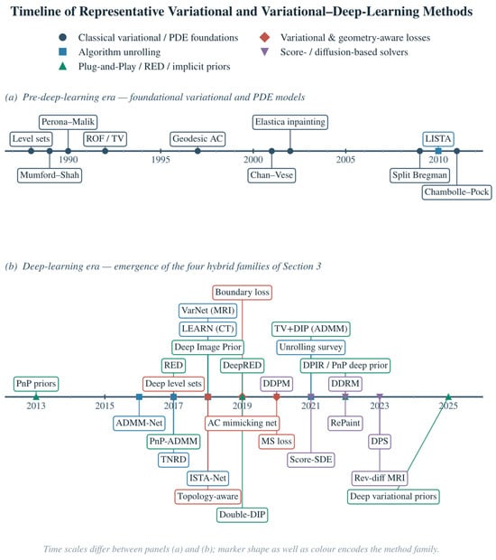
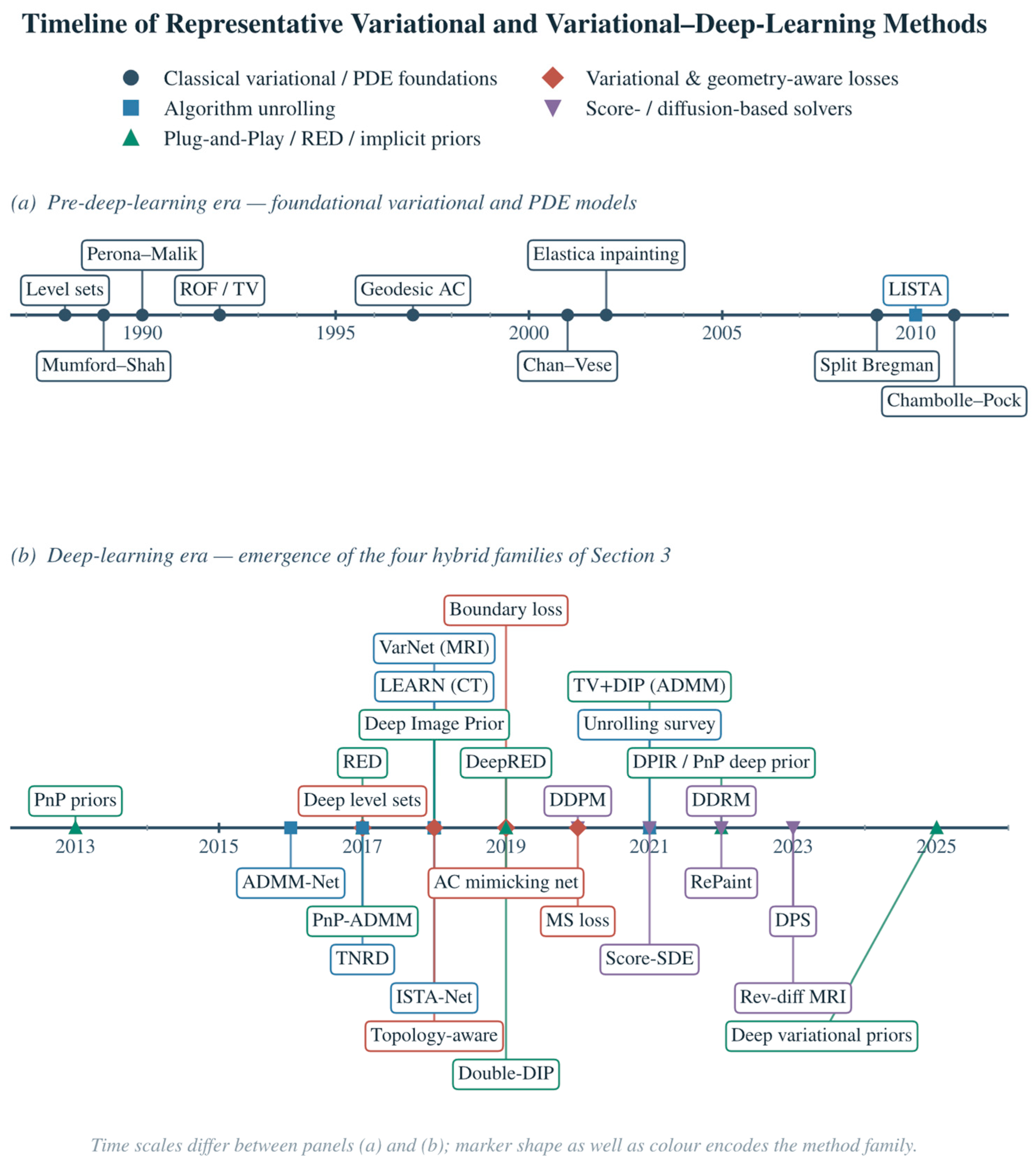
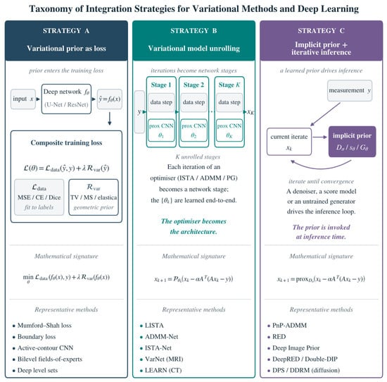

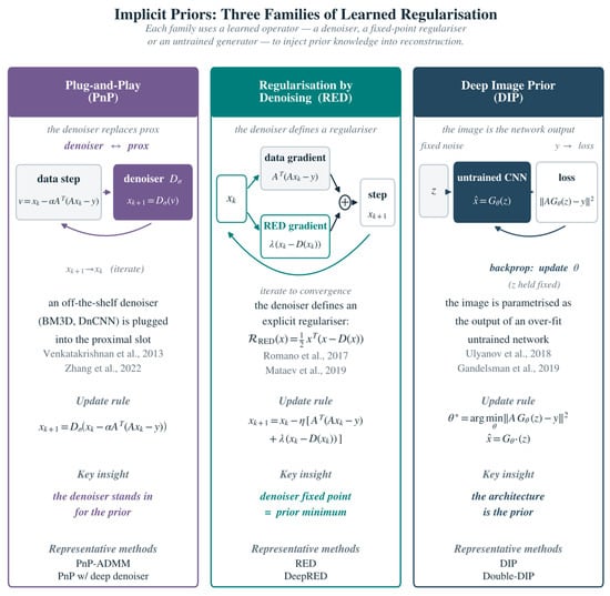
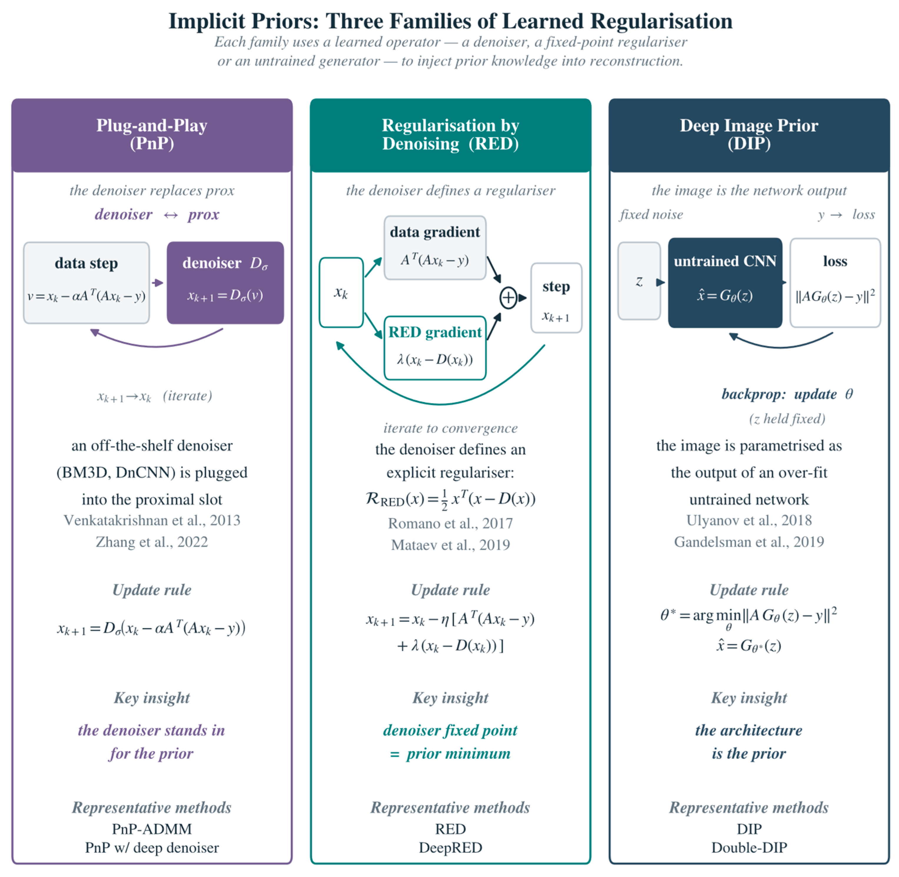
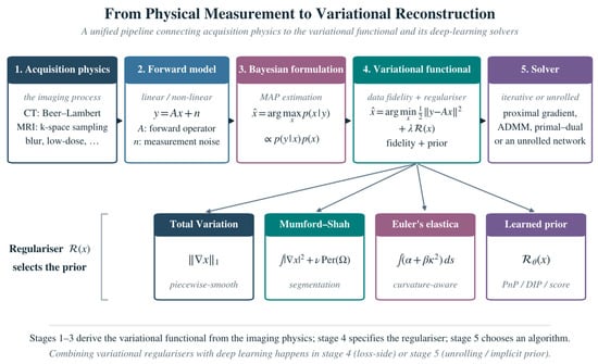
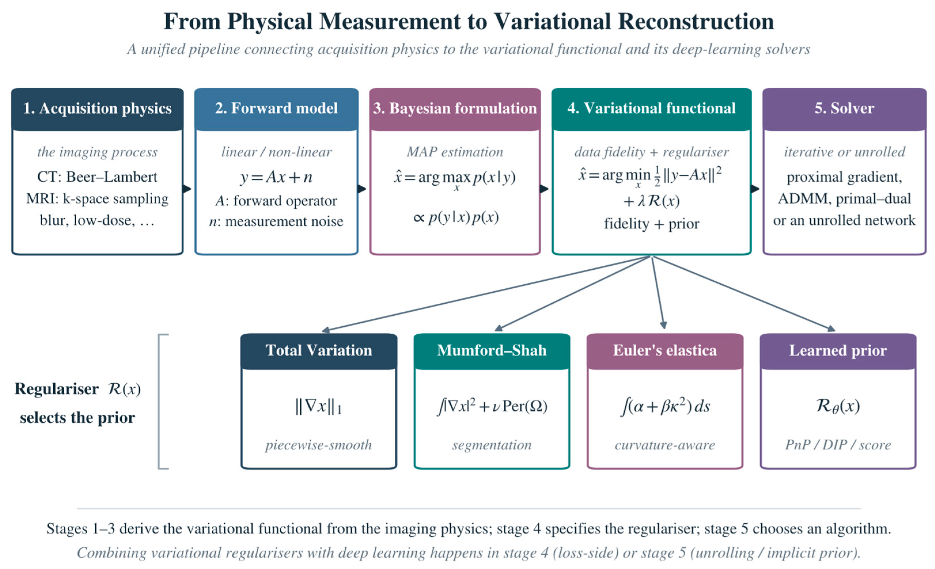
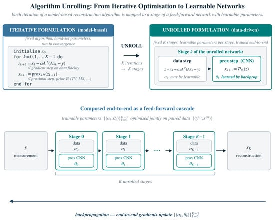
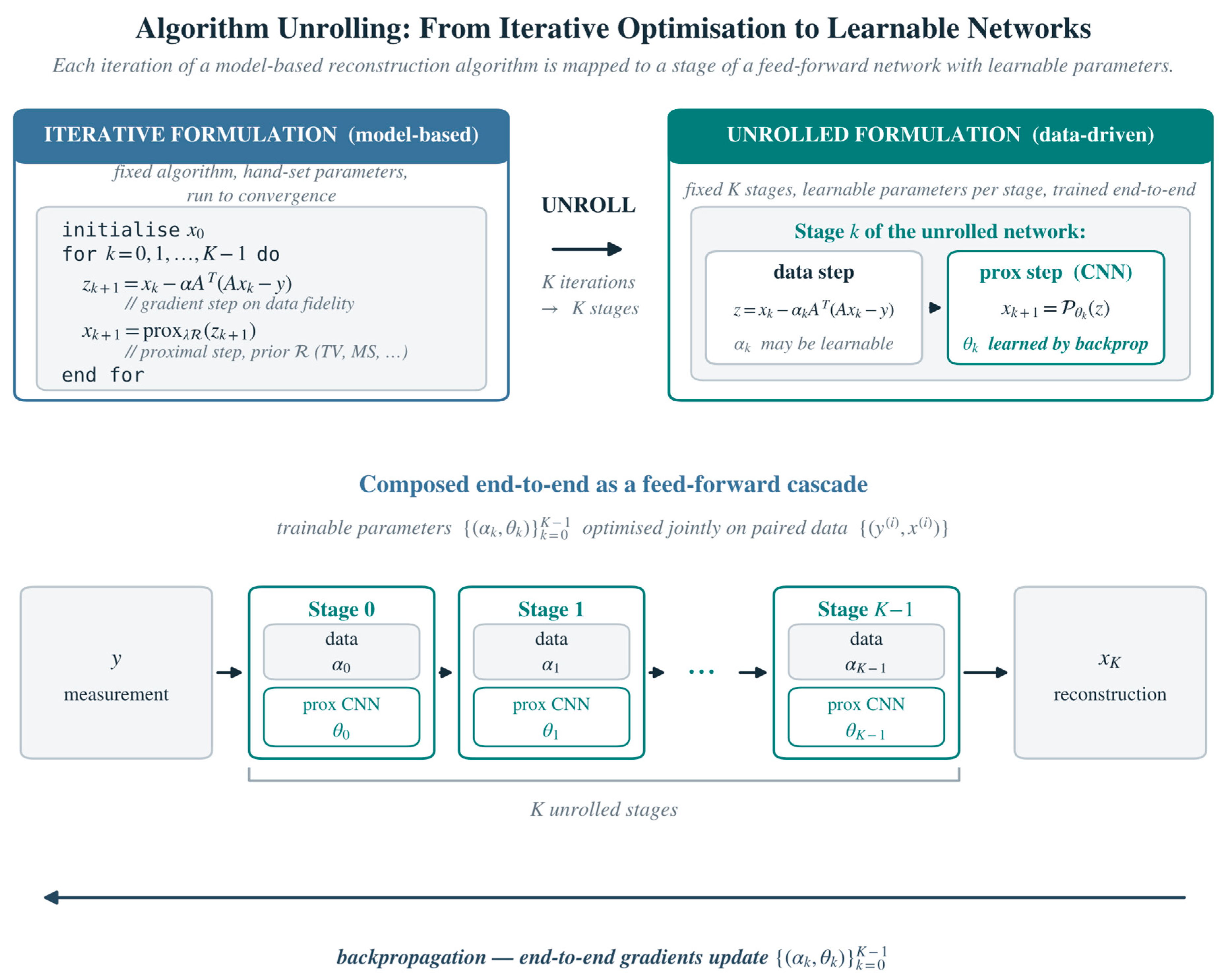

Disclaimer/Publisher’s Note: The statements, opinions and data contained in all publications are solely those of the individual author(s) and contributor(s) and not of MDPI and/or the editor(s). MDPI and/or the editor(s) disclaim responsibility for any injury to people or property resulting from any ideas, methods, instructions or products referred to in the content. |
© 2026 by the authors. Licensee MDPI, Basel, Switzerland. This article is an open access article distributed under the terms and conditions of the Creative Commons Attribution (CC BY) license.