Fuzzy Filtering for Networked Nonlinear Systems with Dynamic Quantization: Quantization-Dependent Event-Triggered Case

Abstract

This paper investigates the event-triggered robust dissipative filtering problem for discrete-time networked nonlinear systems subject to dynamic quantization and stochastic cyber attacks. The networked nonlinear system under consideration is represented by a Takagi-Sugeno (T-S) fuzzy model with parameter uncertainties. A dynamic quantizer and a novel quantization-dependent event-triggered mechanism are introduced to reduce the communication burden, thereby improving the utilization of the limited network resources. Moreover, a Bernoulli-distributed random variable is adopted to characterize the effects of stochastic cyber attacks. Attention is focused on the design of a filter such that the filtering error system is stochastically stable and satisfies a prescribed dissipative performance level. By applying the matrix inequality decoupling approach, the design conditions for the desired dynamic quantizer and filter are obtained in terms of linear matrix inequalities. Finally, simulation results for the Henon mapping system demonstrate that the proposed design approach guarantees the prescribed dissipative performance of $\gamma =1.5$. In addition, the number of triggering events is reduced by 14.13% compared with that of existing quantization-independent methods.

1. Introduction

Over the past few decades, the investigation of networked systems has attracted substantial research interest [1], largely owing to their wide applications in areas including intelligent transportation, robotics, and aerospace. Two primary research directions have emerged within the existing literature on networked systems. The first focuses on developing control strategies for the efficient utilization of limited communication resources. The second concerns the design of security controllers to preserve satisfactory system performance in the presence of cyber attacks. In the first direction, recent years have witnessed growing research attention to networked systems subject to quantization and event-triggered strategies. This is mainly because quantization and event-triggered strategies can markedly reduce the data transmission burden while making efficient use of limited communication resources. Accordingly, numerous important results on networked systems with quantization and event-triggered strategies have been reported in the literature. For instance, quantized control problems for networked systems have been addressed in [2,3,4,5,6,7,8] and event-triggered control problems for networked systems have been investigated in [4,5,6,7,8,9,10,11]. Additionally, many security controller design problems for networked systems under cyber attacks have been studied in [8,9,10].

In recent years, the Takagi-Sugeno (T-S) fuzzy model approach has attracted much attention because of its remarkable advantages in tackling the analysis and design problems of nonlinear systems. In the T-S fuzzy model approach, the considered nonlinear systems can be represented by a set of local linear models connected by IF-THEN rules. Then, the analysis and design problems for nonlinear systems can be addressed based on the well-established linear system theory. As a result, numerous important results have been reported for nonlinear systems by employing the T-S fuzzy model approach. Particularly, by applying the T-S fuzzy model approach, control problems have been investigated for networked nonlinear systems with quantization in [12,13,14,15,16,17,18]; controller design problems have been considered for networked nonlinear systems with different event-triggered schemes in [15,16,17,18,19,20,21,22,23]; and security control problems have been discussed for networked nonlinear systems in the presence of cyber attacks in [16,17,18,19].

In addition, the filtering problem has attracted considerable attention since the state variables of most practical systems are not always available [24,25]. As an important research topic in control theory, the filtering problem has been extensively investigated in recent years, and a great number of important results have been reported. To mention a few, by utilizing the T-S fuzzy model approach, filtering problems have been considered for networked nonlinear systems with quantization in [26,27,28,29,30,31,32,33,34]; filter design problems have been addressed for networked nonlinear systems with various event-triggered schemes in [30,31,32,33,34,35,36,37,38,39,40,41]; and security filtering problems have been discussed for networked nonlinear systems in the presence of cyber attacks in [33,34,39,40,41]. However, it should be noted that most of the above results on filtering problems for networked nonlinear systems have only considered either a quantization scheme or an event-triggered scheme, while few results have investigated the filtering problem with both quantization and event-triggered schemes, especially when quantization, a quantization-dependent event-triggered scheme, and stochastic cyber attacks are taken into account simultaneously. Moreover, even in the existing results that consider both schemes, the quantization and event-triggered strategies have been designed independently of each other, i.e., the event-triggered scheme is quantization-independent. Consequently, the study of the dissipative filtering problem for networked nonlinear systems with dynamic quantization, a quantization-dependent event-triggered strategy, and stochastic cyber attacks, based on the T-S fuzzy model approach, remains both significant and challenging.

In contrast to the existing studies, the contributions of this paper are summarized as follows:

(1)

This paper investigates the robust dissipative filtering problem for discrete-time uncertain networked nonlinear systems with stochastic cyber attacks.

(2)

The dynamic quantization, together with a novel quantization-dependent event-triggered strategy, is adopted to reduce the communication burden and improve the utilization of the limited communication resources.

(3)

The matrix inequality decoupling approach and a dimension-tuning matrix are employed to establish a unified framework in terms of linear matrix inequalities, which is applicable to both full-order and reduced-order filter design.

The remainder of this paper is organized as follows: Section 2 formulates the problem; Section 3 presents the main results; Section 4 provides a simulation example; and Section 5 concludes this paper.

Notations: The identity matrix and zero matrix with compatible dimensions are denoted by I and 0, respectively. $diag\{\cdots \}$ represents a block-diagonal matrix. ${\mathcal{R}}^n$ stands for the n-dimensional vector space. ${\mathcal{R}}^{n\times m}$ denotes the set of all real matrices of dimension $n\times m$. $\mathbf{sym}\left\{A\right\}$ represents $A^T+A$. $\left|·\right|$ indicates the Euclidean vector norm.

2. Problem Formulation

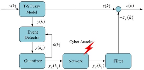
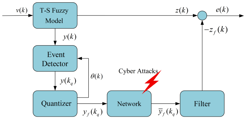
Figure 1 presents a block diagram of the dissipative filtering problem for the networked nonlinear systems considered in this paper, and the problem is mathematically formulated in this section.

Figure 1. Block diagram of the filtering problem for the networked nonlinear systems.

2.1. Nonlinear Plant

In this paper, the following discrete-time uncertain T-S fuzzy model is employed to represent the nonlinear plant under consideration. The $\mathfrak{j}$th rule is formulated as:

$$\begin{array}{c}\mathrm{Plant}\mathrm{Rule}\mathfrak{j}:\mathrm{IF}{\mathfrak{p}}_1\left(k\right)\mathrm{is}{\mathfrak{M}}_{1\mathfrak{j}},{\mathfrak{p}}_2\left(k\right)\mathrm{is}{\mathfrak{M}}_{2\mathfrak{j}}\mathrm{and}\dots \mathrm{and}\hfill \\ {\mathfrak{p}}_{\mathfrak{v}}\left(k\right)\mathrm{is}{\mathfrak{M}}_{\mathfrak{v}\mathfrak{j}},\hfill \\ \mathrm{THEN}x(k+1)=(A_{\mathfrak{j}}+\Delta A_{\mathfrak{j}})x\left(k\right)+(B_{\mathfrak{j}}+\Delta B_{\mathfrak{j}})v\left(k\right)\hfill \\ y\left(k\right)=C_{\mathfrak{j}}x\left(k\right)+D_{\mathfrak{j}}v\left(k\right)\hfill \\ z\left(k\right)=E_{\mathfrak{j}}x\left(k\right)+F_{\mathfrak{j}}v\left(k\right)\hfill \end{array}$$

(1)

where $\mathfrak{p}\left(k\right)=[{\mathfrak{p}}_1\left(k\right),{\mathfrak{p}}_2\left(k\right),...,{\mathfrak{p}}_{\mathfrak{v}}\left(k\right)]$ represents the premise variable, ${\mathfrak{M}}_{\kappa \mathfrak{j}}$ denote the fuzzy sets for $\mathfrak{j}=1,...,r$ and $\kappa =1,...,\mathfrak{v}$, and r is the number of fuzzy rules. $x\left(k\right)\in {\mathcal{R}}^{n_x}$ denotes the state variable of the system, $y\left(k\right)\in {\mathcal{R}}^{n_y}$ is the measurement output, $z\left(k\right)\in {\mathcal{R}}^{n_z}$ is the performance output, and $v\left(k\right)\in {\mathcal{R}}^{n_v}$ is the disturbance input, which belongs to $l_2\left[0,\infty \right)$. $A_{\mathfrak{j}}$, $B_{\mathfrak{j}}$, $C_{\mathfrak{j}}$, $D_{\mathfrak{j}}$, $E_{\mathfrak{j}}$, and $F_{\mathfrak{j}}$ are given system matrices of appropriate dimensions.

The matrices $\Delta A_{\mathfrak{j}}$ and $\Delta B_{\mathfrak{j}}$ represent time-varying norm-bounded parameter uncertainties, which are formulated as

$$\begin{array}{c}[\Delta A_{\mathfrak{j}}\Delta B_{\mathfrak{j}}]=E_{c\mathfrak{j}}{\Delta }_R\left[R_1{R}_2\right]\hfill \end{array}$$

(2)

where ${\Delta }_R$ denotes an unknown matrix satisfying ${\Delta }_R^T{\Delta }_R\le I$, and $E_{c\mathfrak{j}}$ ($\mathfrak{j}=1,\dots ,r$), $R_1$, and $R_2$ are known constant matrices.

For the fuzzy model (1), the fuzzy basis functions can be represented as

$$\begin{array}{c}{\mathfrak{g}}_{\mathfrak{j}}\left(\mathfrak{p}\left(k\right)\right)={\displaystyle \frac{{\prod }_{\kappa =1}^{\mathfrak{v}}{\mathfrak{M}}_{\kappa \mathfrak{j}}\left({\mathfrak{p}}_{\kappa }\left(k\right)\right)}{{\sum }_{\mathfrak{j}=1}^r{\prod }_{\kappa =1}^{\mathfrak{v}}{\mathfrak{M}}_{\kappa \mathfrak{j}}\left({\mathfrak{p}}_{\kappa }\left(k\right)\right)}},\mathfrak{j}=1,\dots ,r\hfill \end{array}$$

(3)

where ${\mathfrak{M}}_{\kappa \mathfrak{j}}\left({\mathfrak{p}}_{\kappa }\left(k\right)\right)$ is the grade of membership of ${\mathfrak{p}}_{\kappa }\left(k\right)$ in ${\mathfrak{M}}_{\kappa \mathfrak{j}}$.

Based on the above definition, we have

$$\begin{array}{c}{\mathfrak{g}}_{\mathfrak{j}}\left(\mathfrak{p}\left(k\right)\right)\ge 0,{\displaystyle {\sum }_{\mathfrak{j}=1}^r}{\mathfrak{g}}_{\mathfrak{j}}\left(\mathfrak{p}\left(k\right)\right)=1,\mathfrak{j}=1,...,r\hfill \end{array}$$

(4)

Then, the T-S fuzzy model (1) can be expressed as

$$\begin{array}{c}x(k+1)=\left(A\right(\mathfrak{g})+\Delta A(\mathfrak{g}\left)\right)x\left(k\right)+\left(B\right(\mathfrak{g})+\Delta B(\mathfrak{g}\left)\right)v\left(k\right)\hfill \\ y\left(k\right)=C\left(\mathfrak{g}\right)x\left(k\right)+D\left(\mathfrak{g}\right)v\left(k\right)\hfill \\ z\left(k\right)=E\left(\mathfrak{g}\right)x\left(k\right)+F\left(\mathfrak{g}\right)v\left(k\right)\hfill \end{array}$$

(5)

where

$$\begin{array}{c}A\left(\mathfrak{g}\right)={\displaystyle \sum _{\mathfrak{j}=1}^r}{\mathfrak{g}}_{\mathfrak{j}}\left(\mathfrak{p}\left(k\right)\right)A_{\mathfrak{j}},\Delta A\left(\mathfrak{g}\right)={\displaystyle \sum _{\mathfrak{j}=1}^r}{\mathfrak{g}}_{\mathfrak{j}}\left(\mathfrak{p}\left(k\right)\right)\Delta A_{\mathfrak{j}},C\left(\mathfrak{g}\right)={\displaystyle \sum _{\mathfrak{j}=1}^r}{\mathfrak{g}}_{\mathfrak{j}}\left(\mathfrak{p}\left(k\right)\right)C_{\mathfrak{j}},\hfill \\ B\left(\mathfrak{g}\right)={\displaystyle \sum _{\mathfrak{j}=1}^r}{\mathfrak{g}}_{\mathfrak{j}}\left(\mathfrak{p}\left(k\right)\right)B_{\mathfrak{j}},\Delta B\left(\mathfrak{g}\right)={\displaystyle \sum _{\mathfrak{j}=1}^r}{\mathfrak{g}}_{\mathfrak{j}}\left(\mathfrak{p}\left(k\right)\right)\Delta B_{\mathfrak{j}},D\left(\mathfrak{g}\right)={\displaystyle \sum _{\mathfrak{j}=1}^r}{\mathfrak{g}}_{\mathfrak{j}}\left(\mathfrak{p}\left(k\right)\right)D_{\mathfrak{j}},\hfill \\ E\left(\mathfrak{g}\right)={\displaystyle \sum _{\mathfrak{j}=1}^r}{\mathfrak{g}}_{\mathfrak{j}}\left(\mathfrak{p}\left(k\right)\right)E_{\mathfrak{j}},F\left(\mathfrak{g}\right)={\displaystyle \sum _{\mathfrak{j}=1}^r}{\mathfrak{g}}_{\mathfrak{j}}\left(\mathfrak{p}\left(k\right)\right)F_{\mathfrak{j}}.\hfill \end{array}$$

2.2. Event-Triggered Communication Scheme

In this paper, we propose a novel quantization-dependent event-triggered communication scheme to reduce the frequency of data transmission and alleviate network congestion. As depicted in Figure 1, the measurement output $y\left(k\right)$ is transmitted to the dynamic quantizer whenever the following event-triggered condition

$$\varphi y^T\left(k_q\right){\wedge }_{2}y\left(k_q\right)+\lambda {\theta }^2\left(k\right){\Delta }^2-{\alpha }^T\left(k\right){\wedge }_1\alpha \left(k\right)\le 0$$

(6)

is satisfied. In addition, $y\left(k\right)$ stands for the current measurement output, $y\left(k_q\right)$ indicates the last transmitted measurement output, and $\alpha \left(k\right)=y\left(k\right)-y\left(k_q\right)$. ${\wedge }_1>0$ and ${\wedge }_2>0$ stand for two undetermined parameter matrices, $\varphi \in [0,1)$ and $\lambda$ denote two given constants, while $\theta \left(k\right)$ and $\Delta$ are two parameters of the dynamic quantizer, to be introduced in the next subsequent section.

Remark 1.

This paper develops a novel quantization-dependent event-triggered scheme for networked systems with dynamic quantization, which effectively reduces the communication burden, thereby improving the utilization of bandwidth-limited network resources. It can be observed that the event-triggered condition (6) explicitly incorporates the quantizer parameter $\theta \left(k\right)$, allowing the triggering threshold to adapt to the quantization error bound. When $\theta \left(k\right)$ is large (i.e., coarse quantization), the term $\lambda {\theta }^2\left(k\right){\Delta }^2$ enlarges the triggering threshold, thereby avoiding unnecessary transmissions of output variations whose magnitudes are comparable to the quantization error. Conversely, when $\theta \left(k\right)$ is small (i.e., fine quantization), the threshold shrinks accordingly to maintain the triggering sensitivity and hence the estimation accuracy. This co-design avoids the conservatism of a fixed threshold that must accommodate the worst-case quantization error at all times. In contrast with the quantization-independent event-triggered schemes proposed in [15,16,17,33,34], the proposed quantization-dependent scheme in (6) is more general. It is noted that the quantization-independent scheme adopted in [15,34] can be obtained from the quantization-dependent event-triggered strategy developed in (6) by setting $\lambda =0$. Furthermore, by selecting ${\wedge }_1={\wedge }_2$ together with $\lambda =0$, the quantization-dependent event-triggered strategy developed in (6) reduces to the event-triggered scheme employed in [31,33]. The above advantages will be further verified by the simulation results.

2.3. Dynamic Quantizer

To further reduce the amount of data in the communication network and improve the utilization of the limited communication resources, the dynamic quantization scheme in [2,3,4,5,6,7,12,13,15,16,17] is employed in this paper. As in [2,3,4,5,6,7,12,13,15,16,17], the dynamic quantizer considered herein is given as

$$y_f\left(k_q\right)=\theta \left(k\right)f\left({\displaystyle \frac{y\left(k_q\right)}{\theta \left(k\right)}}\right),\theta \left(k\right)>0$$

(7)

in which $\theta \left(k\right)$ stands for an undetermined parameter of the quantizer, and $f(★)$ indicates a static quantizer satisfying the following two constraints.

$$\left|f\right(\vartheta )-\vartheta |\le \Delta ,\mathrm{IF}\left|\vartheta \right|\le M$$

(8)

$$\left|f\right(\vartheta \left)\right|>M-\Delta ,\mathrm{IF}\left|\vartheta \right|>M$$

(9)

where $\Delta$ denotes the quantization error bound of $f\left(\vartheta \right)-\vartheta$ and M refers to the range of the quantizer $f(★)$.

Remark 2.

The dynamic quantization scheme is advantageous since it dynamically scales the quantization levels to enlarge the region of attraction and attenuate the steady-state limit cycle. As a result, the dynamic quantization scheme in [2,3,4,5,6,7,12,13,15,16,17], rather than the static one in [8,14,18,26,27,30,31], is employed in this paper to further reduce the communication burden.

2.4. Cyber-Attacks

Considering that the quantized measurement output is transmitted to the filter via the unprotected communication network, the phenomenon of stochastic cyber attacks is addressed in this subsection. The quantized measurement output under stochastic cyber attacks is formulated as

$${\overline{y}}_f\left(k_q\right)=\mu C\left(\mathfrak{g}\right)s\left(x\left(k\right)\right)+(1-\mu )y_f\left(k_q\right)$$

(10)

where $s\left(x\right(k\left)\right)$ is a nonlinear function denoting the deception attacks. As in [8,9,10,17,18,33,34], it is assumed that $s\left(x\right(k\left)\right)$ satisfies the following inequality:

$$s^T\left(x\left(k\right)\right)s\left(x\left(k\right)\right)\le x^T\left(k\right)G^{T}Gx\left(k\right)$$

(11)

where G is a given constant matrix for $s\left(x\right(k\left)\right)$. Furthermore, $\mu$ is a Bernoulli random variable with the following statistical characteristics:

$$\begin{array}{c}Prob\{\mu =1\}=\mathbf{E}\left\{\mu \right\}=\overline{\mu }\hfill \\ Prob\{\mu =0\}=1-\overline{\mu }\hfill \end{array}$$

(12)

where $0\le \overline{\mu }\le 1$ is a given scalar.

2.5. Filter

For the event-triggered dissipative filtering problem addressed in this paper, a general filter is constructed to estimate the performance output based on the measurement output. The filter is given as follows:

$$\begin{array}{c}{x}_f(k+1)=A_f{x}_f\left(k\right)+B_f{\overline{y}}_f\left(k_q\right)\hfill \\ z_f\left(k\right)=E_f{x}_f\left(k\right)+F_f{\overline{y}}_f\left(k_q\right)\hfill \end{array}$$

(13)

in which $x_f\left(k\right)\in {\mathcal{R}}^{n_{x_f}}$ indicates the state of the filter and $z_f\left(k\right)\in {\mathcal{R}}^{n_z}$ stands for the output of the filter. The matrices $A_f$, $B_f$, $E_f$, and $F_f$ represent the filter parameters to be designed. Additionally, it is worth noting that the filter in (13) indicates the full-order filter if $n_{x_f}=n_x$ and the reduced-order filter if $1\le n_{x_f}<n_x$.

2.6. Filtering Error System

By defining $\tilde{\mu }=\mu -\overline{\mu }$, ${\eta }^T\left(k\right)=\left[x^T\left(k\right)x_f^T\left(k\right)\right]$, $e\left(k\right)=z\left(k\right)-z_f\left(k\right)$, and $\epsilon \left(k\right)=\theta \left(k\right)\left(f\left({\displaystyle \frac{y\left(k_q\right)}{\theta \left(k\right)}}\right)-{\displaystyle \frac{y\left(k_q\right)}{\theta \left(k\right)}}\right)$ and considering (5), (10), and (13), we can obtain the filtering error system as

$$\begin{array}{c}\eta (k+1)=({\overline{\mathbb{A}}}_1+\tilde{\mu }{\overline{\mathbb{A}}}_2)\eta \left(k\right)+({\overline{\mathbb{B}}}_1+\tilde{\mu }{\overline{\mathbb{B}}}_2)v\left(k\right)+({\overline{\mathbb{C}}}_1+\tilde{\mu }{\overline{\mathbb{C}}}_2)s\left(x\left(k\right)\right)\hfill \\ +({\overline{\mathbb{D}}}_1+\tilde{\mu }{\overline{\mathbb{D}}}_2)\epsilon \left(k\right)-({\overline{\mathbb{D}}}_1+\tilde{\mu }{\overline{\mathbb{D}}}_2)\alpha \left(k\right)\hfill \\ e\left(k\right)=({\overline{\mathbb{F}}}_1+\tilde{\mu }{\overline{\mathbb{F}}}_2)\eta \left(k\right)+({\overline{\mathbb{G}}}_1+\tilde{\mu }{\overline{\mathbb{G}}}_2)v\left(k\right)+({\overline{\mathbb{H}}}_1+\tilde{\mu }{\overline{\mathbb{H}}}_2)s\left(x\left(k\right)\right)\hfill \\ +({\overline{\mathbb{U}}}_1+\tilde{\mu }{\overline{\mathbb{U}}}_2)\epsilon \left(k\right)-({\overline{\mathbb{U}}}_1+\tilde{\mu }{\overline{\mathbb{U}}}_2)\alpha \left(k\right)\hfill \end{array}$$

(14)

where

$$\begin{array}{c}{\overline{\mathbb{A}}}_1=\left[\begin{array}{cc}{A}_{\Delta }& 0\\ (1-\overline{\mu })B_{f}C\left(\mathfrak{g}\right)& A_f\end{array}\right],{\overline{\mathbb{A}}}_2=\left[\begin{array}{cc}0& 0\\ -B_{f}C\left(\mathfrak{g}\right)& 0\end{array}\right],{\overline{\mathbb{B}}}_1=\left[\begin{array}{c}{B}_{\Delta }\\ (1-\overline{\mu })B_{f}D\left(\mathfrak{g}\right)\end{array}\right],\hfill \\ {\overline{\mathbb{B}}}_2=\left[\begin{array}{c}0\\ -B_{f}D\left(\mathfrak{g}\right)\end{array}\right],{\overline{\mathbb{C}}}_1=\left[\begin{array}{c}0\\ \overline{\mu }{B}_{f}C\left(\mathfrak{g}\right)\end{array}\right],{\overline{\mathbb{C}}}_2=\left[\begin{array}{c}0\\ B_{f}C\left(\mathfrak{g}\right)\end{array}\right],{\overline{\mathbb{D}}}_1=\left[\begin{array}{c}0\\ (1-\overline{\mu })B_f\end{array}\right],\hfill \\ {\overline{\mathbb{D}}}_2=\left[\begin{array}{c}0\\ -B_f\end{array}\right],{\overline{\mathbb{F}}}_1=[E\left(\mathfrak{g}\right)-(1-\overline{\mu })F_{f}C\left(\mathfrak{g}\right)-E_f],{\overline{\mathbb{F}}}_2=\left[F_{f}C\left(\mathfrak{g}\right)0\right],\hfill \\ {\overline{\mathbb{U}}}_1=-(1-\overline{\mu })F_f,{\overline{\mathbb{H}}}_1=-\overline{\mu }{F}_{f}C\left(\mathfrak{g}\right),{\overline{\mathbb{H}}}_2=-F_{f}C\left(\mathfrak{g}\right),{\overline{\mathbb{G}}}_2=F_{f}D\left(\mathfrak{g}\right),\hfill \\ {\overline{\mathbb{U}}}_2=F_f,{\overline{\mathbb{G}}}_1=F\left(\mathfrak{g}\right)-(1-\overline{\mu })F_{f}D\left(\mathfrak{g}\right),A_{\Delta }=A\left(\mathfrak{g}\right)+\Delta A\left(\mathfrak{g}\right),\hfill \\ B_{\Delta }=B\left(\mathfrak{g}\right)+\Delta B\left(\mathfrak{g}\right).\hfill \end{array}$$

As prerequisites for formulating the problem considered in this paper, the fundamental concepts of stochastic stability and dissipativity are introduced in the following definitions.

Definition 1

([29,33,34]). For any initial condition, if there exists a finite $\mathbb{W}>0$ satisfying

$$\begin{array}{c}\mathbf{E}\left\{{\displaystyle {\sum }_{k=0}^{\infty }}{\left|\eta \left(k\right)\right|}^2|\eta \left(0\right)\right\}<{\eta }^T\left(0\right)\mathbb{W}\eta \left(0\right)\hfill \end{array}$$

(15)

then the filtering error system (14) is stochastically stable with $v\left(k\right)=0$.

Definition 2

([31,34,37]). For given matrices $X_1=X_1^T\in {\mathcal{R}}^{n_z\times n_z}\le 0$, $X_2\in {\mathcal{R}}^{n_z\times n_v}$, $X_3=X_3^T\in {\mathcal{R}}^{n_v\times n_v}$, where $-X_1={\overline{X}}_1^T{\overline{X}}_1$ and ${\overline{X}}_1\in {\mathcal{R}}^{n_z\times n_z}\ge 0$. The filtering error system (14) is dissipative with a guaranteed dissipative performance γ for zero initial condition, if the following inequality

$$\begin{array}{c}{\displaystyle {\sum }_{k=0}^w}(e^T\left(k\right)X_{1}e\left(k\right)+\mathbf{sym}\left\{e^T\left(k\right)X_{2}v\left(k\right)\right\}\hfill \\ +v^T\left(k\right)(X_3-\gamma I)v\left(k\right))\ge 0\hfill \end{array}$$

(16)

is satisfied for $w>0$.

Remark 3.

It should be noted that the dissipative filtering performance defined in Definition 2 covers several special cases by selecting appropriate parameters. Specifically, the ${\mathcal{H}}_{\infty }$ filtering performance considered in [26,27,29,30,32,33,39] and the passive filtering performance can be obtained by setting $X_1=-I$, $X_2=0$, $X_3=(\gamma +{\gamma }^2)I$ and $X_1=0$, $X_2=I$, $X_3=2\gamma I$, respectively. Moreover, the mixed passive/${\mathcal{H}}_{\infty }$ filtering performance addressed in [38] can be obtained from the dissipative filtering performance defined in Definition 2 by selecting $X_1=-\varrho I$, $X_2=(1-\varrho )I$, $X_3=(2\gamma +\varrho ({\gamma }^2-\gamma ))I$ with $0\le \varrho \le 1$.

The dissipative filtering problem considered in this paper is to design the filter in (13) such that the filtering error system (14) satisfies the following two requirements:

(1)

The filtering error system (14) is stochastically stable in the sense of Definition 1.

(2)

The filtering error system (14) is dissipative in the sense of Definition 2 with a prescribed dissipative performance $\gamma$.

Before establishing the main results of this paper, we first introduce the following two essential lemmas.

Lemma 1

([26,27,29,30]). For real matrices ${\varpi }_1={\varpi }_1^T$, ${\varpi }_2$, ${\varpi }_3$ of appropriate dimensions and ℏ satisfying ${\hslash }^T\hslash \le I$, it can be concluded that ${\varpi }_1+{\varpi }_2\hslash {\varpi }_3+{\varpi }_3^T{\hslash }^T{\varpi }_2^T<0$ if and only if there exists a scalar $\varsigma >0$ such that

$$\begin{array}{c}{\varpi }_1+{\varsigma }^{-1}{\varpi }_2{\varpi }_2^T+\varsigma {\varpi }_3^T{\varpi }_3<0.\hfill \end{array}$$

(17)

Lemma 2

([15,28,34]). For real matrices ${\mathcal{M}}_1$, ${\mathcal{M}}_2$, and ${\mathcal{M}}_3$ of appropriate dimensions, it can be concluded that ${\mathcal{M}}_1+{\mathcal{M}}_2{\mathcal{M}}_3+{\mathcal{M}}_3^T{\mathcal{M}}_2^T<0$ if there exists a matrix ${\mathcal{M}}_4$ such that

$$\begin{array}{c}\left[\begin{array}{cc}{\mathcal{M}}_1& \ast \\ {\mathcal{M}}_2^T+{\mathcal{M}}_4{\mathcal{M}}_3& -{\mathcal{M}}_4-{\mathcal{M}}_4^T\end{array}\right]<0.\hfill \end{array}$$

(18)

3. Main Results

3.1. Filtering Performance Analysis

In this subsection, the dissipative filtering performance analysis problem is investigated. More specifically, a sufficient condition guaranteeing the stochastic stability and the prescribed dissipative filtering performance for the filtering error system (14) is established in the following theorem based on the Lyapunov methodology.

Theorem 1.

Suppose that the constants ϕ, $\overline{\mu }$, M, λ, and Δ, the matrices $X_1=X_1^T\le 0$, $X_2$, and $X_3=X_3^T$, and the filter parameters $A_f$, $B_f$, $E_f$, and $F_f$ are given. The stochastic stability and the prescribed dissipative performance γ of the filtering error system (14) are guaranteed if there exist matrices S, $P>0$, ${\wedge }_1>0$, ${\wedge }_2>0$ and a constant $\psi >1$ satisfying

$$\left[\begin{array}{ccccccc}{Y}_{11}& \ast & \ast & \ast & \ast & \ast & \ast \\ Y_{21}& Y_{22}& \ast & \ast & \ast & \ast & \ast \\ Y_{31}& 0& Y_{22}& \ast & \ast & \ast & \ast \\ Y_{41}& 0& 0& -I& \ast & \ast & \ast \\ Y_{51}& 0& 0& 0& -\lambda I& \ast & \ast \\ Y_{61}& 0& 0& 0& 0& -I& \ast \\ Y_{71}& 0& 0& 0& 0& 0& -I\end{array}\right]<0$$

(19)

where $Y_{22}=P-S^T-S$,

$$\begin{array}{c}{Y}_{11}=\left[\begin{array}{ccccc}{\partial }_{11}& \ast & \ast & \ast & \ast \\ {\partial }_{21}& {\partial }_{22}& \ast & \ast & \ast \\ 0& {\partial }_{32}& -I& \ast & \ast \\ 0& {\partial }_{42}& 0& -I& \ast \\ {\partial }_{51}& {\partial }_{52}& 0& 0& {\partial }_{55}\end{array}\right],\hfill \\ Y_{41}=\left[{\displaystyle \frac{\psi \Delta }{M}}\tilde{C}{\displaystyle \frac{\psi \Delta }{M}}D\left(\mathfrak{g}\right)00-{\displaystyle \frac{\psi \Delta }{M}}I\right],\hfill \\ Y_{21}=\left[S^T{\overline{\mathbb{A}}}_1{S}^T{\overline{\mathbb{B}}}_1{S}^T{\overline{\mathbb{C}}}_1{S}^T{\overline{\mathbb{D}}}_1-S^T{\overline{\mathbb{D}}}_1\right],\hfill \\ Y_{51}=\left[\lambda {\displaystyle \frac{\psi \Delta }{M}}\tilde{C}\lambda {\displaystyle \frac{\psi \Delta }{M}}D\left(\mathfrak{g}\right)00-\lambda {\displaystyle \frac{\psi \Delta }{M}}I\right],\hfill \\ Y_{61}=\left[{\overline{X}}_1{\overline{\mathbb{F}}}_1{\overline{X}}_1{\overline{\mathbb{G}}}_1{\overline{X}}_1{\overline{\mathbb{H}}}_1{\overline{X}}_1{\overline{\mathbb{U}}}_1-{\overline{X}}_1{\overline{\mathbb{U}}}_1\right],\hfill \\ Y_{31}=\left[\widehat{\mu }{S}^T{\overline{\mathbb{A}}}_2\widehat{\mu }{S}^T{\overline{\mathbb{B}}}_2\widehat{\mu }{S}^T{\overline{\mathbb{C}}}_2\widehat{\mu }{S}^T{\overline{\mathbb{D}}}_2-\widehat{\mu }{S}^T{\overline{\mathbb{D}}}_2\right],\hfill \\ Y_{71}=\left[\widehat{\mu }{\overline{X}}_1{\overline{\mathbb{F}}}_2\widehat{\mu }{\overline{X}}_1{\overline{\mathbb{G}}}_2\widehat{\mu }{\overline{X}}_1{\overline{\mathbb{H}}}_2\widehat{\mu }{\overline{X}}_1{\overline{\mathbb{U}}}_2-\widehat{\mu }{\overline{X}}_1{\overline{\mathbb{U}}}_2\right]\hfill \end{array}$$

with ${\partial }_{11}=-P+\varphi {\tilde{C}}^T{\wedge }_2\tilde{C}+{\tilde{G}}^T\tilde{G}$, ${\partial }_{21}=-X_2^T{\overline{\mathbb{F}}}_1+\varphi D{\left(\mathfrak{g}\right)}^T{\wedge }_2\tilde{C}$, ${\partial }_{22}=-(X_3-\gamma I)-X_2^T{\overline{\mathbb{G}}}_1-{\overline{\mathbb{G}}}_1^T{X}_2+\varphi D{\left(\mathfrak{g}\right)}^T{\wedge }_{2}D\left(\mathfrak{g}\right)$, ${\partial }_{32}=-{\overline{\mathbb{H}}}_1^T{X}_2$, ${\partial }_{42}=-{\overline{\mathbb{U}}}_1^T{X}_2$, ${\partial }_{51}=-\varphi {\wedge }_2\tilde{C}$, ${\partial }_{52}={\overline{\mathbb{U}}}_1^T{X}_2-\varphi {\wedge }_{2}D\left(\mathfrak{g}\right)$, ${\partial }_{55}=-{\wedge }_1+\varphi {\wedge }_2$, $\tilde{C}=\left[C\left(\mathfrak{g}\right)0\right]$, $\tilde{G}=\left[G0\right]$, $\widehat{\mu }={\left(\overline{\mu }(1-\overline{\mu })\right)}^{1/2}$.

Proof. 

Considering that $P-S-S^T\ge -S^T{P}^{-1}S$ and performing a congruence transformation to the inequality (19) by $diag\{I,S^{-T},S^{-T},I,$${\lambda }^{-1}I,I,I\}$, we obtain

$$\left[\begin{array}{ccccccc}{Y}_{11}& \ast & \ast & \ast & \ast & \ast & \ast \\ {\overline{Y}}_{21}& -P^{-1}& \ast & \ast & \ast & \ast & \ast \\ {\overline{Y}}_{31}& 0& -P^{-1}& \ast & \ast & \ast & \ast \\ Y_{41}& 0& 0& -I& \ast & \ast & \ast \\ {\overline{Y}}_{51}& 0& 0& 0& -{\lambda }^{-1}I& \ast & \ast \\ Y_{61}& 0& 0& 0& 0& -I& \ast \\ Y_{71}& 0& 0& 0& 0& 0& -I\end{array}\right]<0$$

(20)

where

$$\begin{array}{c}{\overline{Y}}_{21}=\left[{\overline{\mathbb{A}}}_1{\overline{\mathbb{B}}}_1{\overline{\mathbb{C}}}_1{\overline{\mathbb{D}}}_1-{\overline{\mathbb{D}}}_1\right],\hfill \\ {\overline{Y}}_{31}=\left[\widehat{\mu }{\overline{\mathbb{A}}}_2\widehat{\mu }{\overline{\mathbb{B}}}_2\widehat{\mu }{\overline{\mathbb{C}}}_2\widehat{\mu }{\overline{\mathbb{D}}}_2-\widehat{\mu }{\overline{\mathbb{D}}}_2\right],\hfill \\ {\overline{Y}}_{51}=\left[{\displaystyle \frac{\psi \Delta }{M}}\tilde{C}{\displaystyle \frac{\psi \Delta }{M}}D\left(\mathfrak{g}\right)00-{\displaystyle \frac{\psi \Delta }{M}}I\right].\hfill \end{array}$$

To proceed with the derivation, the Lyapunov function is constructed as

$$V\left(\eta \left(k\right)\right)={\eta }^T\left(k\right)P\eta \left(k\right),P>0.$$

(21)

Then, it can be obtained that

$$\begin{array}{c}\mathbf{E}\left\{V\left(\eta (k+1)\right)-V\left(\eta \left(k\right)\right)-e^T\left(k\right)X_{1}e\left(k\right)-e^T\left(k\right)\right.\hfill \\ \left.\times X_{2}v\left(k\right)-v^T\left(k\right)X_2^{T}e\left(k\right)\right\}-v^T\left(k\right)(X_3-\gamma I)v\left(k\right)\hfill \\ ={\widehat{\eta }}^T\left(k\right)\mathbf{E}\{{([{\overline{\mathbb{A}}}_1{\overline{\mathbb{B}}}_1{\overline{\mathbb{C}}}_1{\overline{\mathbb{D}}}_1-{\overline{\mathbb{D}}}_1]+\tilde{\mu }[{\overline{\mathbb{A}}}_2{\overline{\mathbb{B}}}_2{\overline{\mathbb{C}}}_2{\overline{\mathbb{D}}}_2-{\overline{\mathbb{D}}}_2])}^T\hfill \\ \times P([{\overline{\mathbb{A}}}_1{\overline{\mathbb{B}}}_1{\overline{\mathbb{C}}}_1{\overline{\mathbb{D}}}_1-{\overline{\mathbb{D}}}_1]+\tilde{\mu }[{\overline{\mathbb{A}}}_2{\overline{\mathbb{B}}}_2{\overline{\mathbb{C}}}_2{\overline{\mathbb{D}}}_2-{\overline{\mathbb{D}}}_2])\hfill \\ -{([{\overline{\mathbb{F}}}_1{\overline{\mathbb{G}}}_1{\overline{\mathbb{H}}}_1{\overline{\mathbb{U}}}_1-{\overline{\mathbb{U}}}_1]+\tilde{\mu }[{\overline{\mathbb{F}}}_2{\overline{\mathbb{G}}}_2{\overline{\mathbb{H}}}_2{\overline{\mathbb{U}}}_2-{\overline{\mathbb{U}}}_2])}^T{X}_1\hfill \\ \times ([{\overline{\mathbb{F}}}_1{\overline{\mathbb{G}}}_1{\overline{\mathbb{H}}}_1{\overline{\mathbb{U}}}_1-{\overline{\mathbb{U}}}_1]+\tilde{\mu }[{\overline{\mathbb{F}}}_2{\overline{\mathbb{G}}}_2{\overline{\mathbb{H}}}_2{\overline{\mathbb{U}}}_2-{\overline{\mathbb{U}}}_2])\hfill \\ -{([{\overline{\mathbb{F}}}_1{\overline{\mathbb{G}}}_1{\overline{\mathbb{H}}}_1{\overline{\mathbb{U}}}_1-{\overline{\mathbb{U}}}_1]+\tilde{\mu }[{\overline{\mathbb{F}}}_2{\overline{\mathbb{G}}}_2{\overline{\mathbb{H}}}_2{\overline{\mathbb{U}}}_2-{\overline{\mathbb{U}}}_2])}^T{X}_2\hfill \\ \times \left[0I000\right]-{\left[0I000\right]}^T{X}_2^T([{\overline{\mathbb{F}}}_1{\overline{\mathbb{G}}}_1{\overline{\mathbb{H}}}_1{\overline{\mathbb{U}}}_1-{\overline{\mathbb{U}}}_1]\hfill \\ +\tilde{\mu }[{\overline{\mathbb{F}}}_2{\overline{\mathbb{G}}}_2{\overline{\mathbb{H}}}_2{\overline{\mathbb{U}}}_2-{\overline{\mathbb{U}}}_2]\left)\right\}\widehat{\eta }\left(k\right)\hfill \\ -{\widehat{\eta }}^T\left(k\right)diag\{P,X_3-\gamma I,0,0,0\}\widehat{\eta }\left(k\right)\hfill \\ ={\widehat{\eta }}^T\left(k\right)\widehat{Z_0}\widehat{\eta }\left(k\right)\hfill \end{array}$$

(22)

where ${\widehat{\eta }}^T\left(k\right)=\left[{\eta }^T\left(k\right)v^T\left(k\right)s^T\left(x\left(k\right)\right){\epsilon }^T\left(k\right){\alpha }^T\left(k\right)\right]$ and

$$\begin{array}{c}\widehat{Z_0}={[{\overline{\mathbb{A}}}_1{\overline{\mathbb{B}}}_1{\overline{\mathbb{C}}}_1{\overline{\mathbb{D}}}_1-{\overline{\mathbb{D}}}_1]}^{T}P[{\overline{\mathbb{A}}}_1{\overline{\mathbb{B}}}_1{\overline{\mathbb{C}}}_1{\overline{\mathbb{D}}}_1-{\overline{\mathbb{D}}}_1]\hfill \\ +{\widehat{\mu }}^2{[{\overline{\mathbb{A}}}_2{\overline{\mathbb{B}}}_2{\overline{\mathbb{C}}}_2{\overline{\mathbb{D}}}_2-{\overline{\mathbb{D}}}_2]}^{T}P[{\overline{\mathbb{A}}}_2{\overline{\mathbb{B}}}_2{\overline{\mathbb{C}}}_2{\overline{\mathbb{D}}}_2-{\overline{\mathbb{D}}}_2]\hfill \\ -{[{\overline{\mathbb{F}}}_1{\overline{\mathbb{G}}}_1{\overline{\mathbb{H}}}_1{\overline{\mathbb{U}}}_1-{\overline{\mathbb{U}}}_1]}^T{X}_1[{\overline{\mathbb{F}}}_1{\overline{\mathbb{G}}}_1{\overline{\mathbb{H}}}_1{\overline{\mathbb{U}}}_1-{\overline{\mathbb{U}}}_1]\hfill \\ -{\widehat{\mu }}^2{[{\overline{\mathbb{F}}}_2{\overline{\mathbb{G}}}_2{\overline{\mathbb{H}}}_2{\overline{\mathbb{U}}}_2-{\overline{\mathbb{U}}}_2]}^T{X}_1[{\overline{\mathbb{F}}}_2{\overline{\mathbb{G}}}_2{\overline{\mathbb{H}}}_2{\overline{\mathbb{U}}}_2-{\overline{\mathbb{U}}}_2]\hfill \\ -{[{\overline{\mathbb{F}}}_1{\overline{\mathbb{G}}}_1{\overline{\mathbb{H}}}_1{\overline{\mathbb{U}}}_1-{\overline{\mathbb{U}}}_1]}^T{X}_2\left[0I000\right]\hfill \\ -{\left[0I000\right]}^T{X}_2^T[{\overline{\mathbb{F}}}_1{\overline{\mathbb{G}}}_1{\overline{\mathbb{H}}}_1{\overline{\mathbb{U}}}_1-{\overline{\mathbb{U}}}_1]\hfill \\ -diag\{P,X_3-\gamma I,0,0,0\}.\hfill \end{array}$$

By considering the event-triggered condition in (6), it can be deduced that ${\alpha }^T\left(k\right){\wedge }_1\alpha \left(k\right)\le \varphi y^T\left(k_q\right){\wedge }_{2}y\left(k_q\right)+\lambda {\theta }^2\left(k\right){\Delta }^2$. Moreover, we define the parameter of the dynamic quantizer as

$$\begin{array}{c}\theta \left(k\right)={\displaystyle \frac{\psi }{M}}\left|y\left(k_q\right)\right|,\psi \ge 1.\hfill \end{array}$$

(23)

Then, it can be obtained that

$$\begin{array}{c}{\widehat{\eta }}^T\left(k\right)\widehat{Z_1}\widehat{\eta }\left(k\right)\ge 0\hfill \end{array}$$

(24)

where

$$\begin{array}{c}\widehat{Z_1}=\varphi {[\tilde{C}D\left(\mathfrak{g}\right)00-I]}^T{\wedge }_2[\tilde{C}D\left(\mathfrak{g}\right)00-I]\hfill \\ +\lambda {[{\displaystyle \frac{\psi \Delta }{M}}\tilde{C}{\displaystyle \frac{\psi \Delta }{M}}D\left(\mathfrak{g}\right)00-{\displaystyle \frac{\psi \Delta }{M}}I]}^T[{\displaystyle \frac{\psi \Delta }{M}}\tilde{C}{\displaystyle \frac{\psi \Delta }{M}}D\left(\mathfrak{g}\right)00-{\displaystyle \frac{\psi \Delta }{M}}I]\hfill \\ -diag\{0,0,0,0,{\wedge }_1\}.\hfill \end{array}$$

Next, combining the property of the quantizer $f(★)$ given in (8) and the definition of $\theta \left(k\right)$ in (23), we deduce that ${\epsilon }^T\left(k\right)\epsilon \left(k\right)\le {\displaystyle \frac{{\psi }^2{\Delta }^2}{M^2}}{y}^T\left(k_q\right)y\left(k_q\right)$, from which we further obtain

$$\begin{array}{c}{\widehat{\eta }}^T\left(k\right)\widehat{Z_2}\widehat{\eta }\left(k\right)\ge 0\hfill \end{array}$$

(25)

where

$$\begin{array}{c}\widehat{Z_2}={[{\displaystyle \frac{\psi \Delta }{M}}\tilde{C}{\displaystyle \frac{\psi \Delta }{M}}D\left(\mathfrak{g}\right)00-{\displaystyle \frac{\psi \Delta }{M}}I]}^T[{\displaystyle \frac{\psi \Delta }{M}}\tilde{C}{\displaystyle \frac{\psi \Delta }{M}}D\left(\mathfrak{g}\right)00-{\displaystyle \frac{\psi \Delta }{M}}I]\hfill \\ -diag\{0,0,0,I,0\}.\hfill \end{array}$$

Additionally, we can further rewrite the constraint on the cyber attacks given in (11) as

$$\begin{array}{c}{\widehat{\eta }}^T\left(k\right)\widehat{Z_3}\widehat{\eta }\left(k\right)\ge 0\hfill \end{array}$$

(26)

where ${\widehat{Z}}_3={\left[\tilde{G}0000\right]}^T\left[\tilde{G}0000\right]-diag\{0,0,I,0,0\}$.

By applying the Schur complement to the inequality in (20), we obtain

$$\begin{array}{c}\widehat{Z_0}+\widehat{Z_1}+\widehat{Z_2}+\widehat{Z_3}<0.\hfill \end{array}$$

(27)

According to the S-procedure in [3,28], together with the inequalities in (24)–(26), we obtain ${\widehat{\eta }}^T\left(k\right)\widehat{Z_0}\widehat{\eta }\left(k\right)<0$, i.e.,

$$\begin{array}{c}\mathbf{E}\{V\left(\eta (k+1)\right)-V\left(\eta \left(k\right)\right)-e^T\left(k\right)X_{1}e\left(k\right)-e^T\left(k\right)X_{2}v\left(k\right)\hfill \\ -v^T\left(k\right)X_2^{T}e\left(k\right)\}-v^T\left(k\right)(X_3-\gamma I)v\left(k\right)<0\hfill \end{array}$$

(28)

By summing up the inequality in (28) from $k=0$ to $k=w$, we can conclude that

$$\begin{array}{c}\mathbf{E}\left\{V\left(\eta (w+1)\right)\right\}-V\left(\eta \left(0\right)\right)-{\displaystyle {\sum }_{k=0}^w}\left(\mathbf{E}\right\{e^T\left(k\right)X_1\hfill \\ \times e\left(k\right)+e^T\left(k\right)X_{2}v\left(k\right)+v^T\left(k\right)X_2^{T}e\left(k\right)\}\hfill \\ +v^T\left(k\right)(X_3-\gamma I)v\left(k\right))<0\hfill \end{array}$$

(29)

It should be noted that $V\left(\eta \right(0\left)\right)=0$ and $\mathbf{E}\left\{V\right(\eta (w+1)\left)\right\}\ge 0$. Based on the inequality in (29), we obtain

$$\begin{array}{c}{\displaystyle {\sum }_{k=0}^w}(\mathbf{E}\{e^T\left(k\right)X_{1}e\left(k\right)+e^T\left(k\right)X_{2}v\left(k\right)+v^T\left(k\right)X_2^{T}e\left(k\right)\}\hfill \\ +v^T\left(k\right)(X_3-\gamma I)v\left(k\right))\ge 0\hfill \end{array}$$

(30)

Recalling Definition 2, we deduce that the prescribed dissipative performance $\gamma$ of the filtering error system (14) is guaranteed if the condition in (19) is satisfied.

Next, we prove that if the condition in (19) holds, the filtering error system (14) is stochastically stable under $v\left(k\right)=0$.

For $v\left(k\right)=0$, the inequality in (28) reduces to the following inequality:

$$\begin{array}{c}\mathbf{E}\{\left(\eta (k+1)\right)-V\left(\eta \left(k\right)\right)\}<e^T\left(k\right)X_{1}e\left(k\right).\hfill \end{array}$$

(31)

Noting that $X_1\le 0$, we obtain

$$\begin{array}{c}\mathbf{E}\{\left(\eta (k+1)\right)-V\left(\eta \left(k\right)\right)\}={\tilde{\eta }}^T\left(k\right){\tilde{Z}}_0\tilde{\eta }\left(k\right)<0\hfill \end{array}$$

(32)

where ${\tilde{\eta }}^T\left(k\right)=\left[{\eta }^T\left(k\right)s^T\left(x\left(k\right)\right){\epsilon }^T\left(k\right){\alpha }^T\left(k\right)\right]$ and

$$\begin{array}{c}{\tilde{Z}}_0={[{\overline{\mathbb{A}}}_1{\overline{\mathbb{C}}}_1{\overline{\mathbb{D}}}_1-{\overline{\mathbb{D}}}_1]}^{T}P[{\overline{\mathbb{A}}}_1{\overline{\mathbb{C}}}_1{\overline{\mathbb{D}}}_1-{\overline{\mathbb{D}}}_1]\hfill \\ +{\widehat{\mu }}^2{[{\overline{\mathbb{A}}}_2{\overline{\mathbb{C}}}_2{\overline{\mathbb{D}}}_2-{\overline{\mathbb{D}}}_2]}^{T}P[{\overline{\mathbb{A}}}_2{\overline{\mathbb{C}}}_2{\overline{\mathbb{D}}}_2-{\overline{\mathbb{D}}}_2]\hfill \\ -diag\{P,0,0,0\}.\hfill \end{array}$$

Based on the equation in (32), we obtain

$$\begin{array}{c}\mathbf{E}\{\left(\eta (k+1)\right)-V\left(\eta \left(k\right)\right)\}\le -{\lambda }_{\min }(-{\tilde{Z}}_0){\tilde{\eta }}^T\left(k\right)\tilde{\eta }\left(k\right)\hfill \end{array}$$

(33)

Moreover, for any $\delta \ge 1$, we take mathematical expectation of the inequality (33) and sum both sides from $k=0$ to $k=\delta$. Then, we obtain

$$\begin{array}{c}\mathbf{E}\left\{{\eta }^T(\delta +1)P\eta (\delta +1)\right\}-{\eta }^T\left(0\right)P\eta \left(0\right)\hfill \\ \le -{\lambda }_{\min }(-{\tilde{Z}}_0)\mathbf{E}\left\{{\displaystyle {\sum }_{k=0}^{\delta }}\left|\tilde{\eta }{\left(k\right)}^2\right|\right\}\hfill \end{array}$$

(34)

which implies

$$\begin{array}{c}\mathbf{E}\left\{{\displaystyle {\sum }_{k=0}^{\delta }}{\left|\tilde{\eta }\left(k\right)\right|}^2\right\}\le {\left({\lambda }_{\min }(-{\tilde{Z}}_0)\right)}^{-1}({\eta }^T\left(0\right)P\eta \left(0\right)\hfill \\ -\mathbf{E}\left\{{\eta }^T(\delta +1)P\eta (\delta +1)\right\}).\hfill \end{array}$$

(35)

Letting $\delta \to \infty$, one deduces that $\mathbf{E}\left\{{\sum }_{k=0}^{\infty }\left|\tilde{\eta }{\left(k\right)}^2\right|\right\}\ge \mathbf{E}\left\{{\sum }_{k=0}^{\infty }\left|\eta {\left(k\right)}^2\right|\right\}$ and $\mathbf{E}\left\{{\eta }^T(\infty )P\eta (\infty )\right\}\ge 0$. As a result, we further rewrite the inequality in (35) as

$$\begin{array}{c}\mathbf{E}\left\{{\displaystyle {\sum }_{k=0}^{\infty }}\left|\eta {\left(k\right)}^2\right|\right\}\le {\left({\lambda }_{\min }(-{\tilde{Z}}_0)\right)}^{-1}{\eta }^T\left(0\right)P\eta \left(0\right)\hfill \\ ={\eta }^T\left(0\right){\left({\lambda }_{\min }(-{\tilde{Z}}_0)\right)}^{-1}P\eta \left(0\right)\hfill \\ ={\eta }^T\left(0\right)\mathbb{W}\eta \left(0\right)\hfill \end{array}$$

(36)

where $\mathbb{W}={\left({\lambda }_{\min }(-{\tilde{Z}}_0)\right)}^{-1}P$. Based on ${\tilde{\eta }}^T\left(k\right){\tilde{Z}}_0\tilde{\eta }\left(k\right)<0$, we have ${\tilde{Z}}_0<0$, i.e., ${\lambda }_{\min }(-{\tilde{Z}}_0)>0$. Furthermore, we obtain $\mathbb{W}={\left({\lambda }_{\min }(-Z_0)\right)}^{-1}P>0$. Recalling Definition 1, we have that the stochastic stability of the filtering system (14) is guaranteed if the condition (19) is satisfied.

□

3.2. Filter Design

In this subsection, the filter design problem is investigated. More specifically, based on Lemmas 1 and 2, and Theorem 1, the design conditions for the desired event-triggered communication scheme in (6), the dynamic quantizer in (7), and the filter in (13) are presented in terms of linear matrix inequalities.

Theorem 2.

Suppose that the constants ϕ, $\overline{\mu }$, M, λ, Δ, ${\sigma }_1$, ${\sigma }_2$, ${\sigma }_3$, and ${\sigma }_4$, the matrices ${\overline{X}}_1\ge 0$, $X_2$, $X_3=X_3^T$, and Q are given. The stochastic stability and the prescribed dissipative performance γ of the filtering error system (14) are guaranteed if there exist matrices $P_1$, $P_2$, $P_3$, $S_1$, $S_2$, $S_3$, $S_4$, $A_F$, $B_F$, $E_F$, $F_F$, Θ, ${\wedge }_1>0$, ${\wedge }_2>0$ and constants $\psi >1$, $\varsigma >0$ satisfying

$$\begin{array}{c}{\mathrm{\Omega }}_{\mathfrak{j}}<0,\mathfrak{j}=1,\dots ,r\hfill \end{array}$$

(37)

where

$$\begin{array}{c}{\mathrm{\Omega }}_{\mathfrak{j}}=\left[\begin{array}{ccccccc}{\Xi }_{11\mathfrak{j}}& \ast & \ast & \ast & \ast & \ast & \ast \\ {\Xi }_{21\mathfrak{j}}& {\Xi }_{22}& \ast & \ast & \ast & \ast & \ast \\ {\Xi }_{31\mathfrak{j}}& 0& {\Xi }_{22}& \ast & \ast & \ast & \ast \\ {\Xi }_{41\mathfrak{j}}& 0& 0& {\Xi }_{44}& \ast & \ast & \ast \\ 0& {\Xi }_{52\mathfrak{j}}& 0& 0& -\varsigma I& \ast & \ast \\ {\Xi }_{61}& 0& 0& 0& 0& -\varsigma I& \ast \\ {\Xi }_{71\mathfrak{j}}& {\Xi }_{72}& {\Xi }_{73}& 0& 0& 0& {\Xi }_{77}\end{array}\right],\hfill \\ {\Xi }_{11\mathfrak{j}}=\left[\begin{array}{ccccc}{\Gamma }_{11\mathfrak{j}}& \ast & \ast & \ast & \ast \\ {\Gamma }_{21\mathfrak{j}}& {\Gamma }_{22\mathfrak{j}}& \ast & \ast & \ast \\ 0& {\Gamma }_{32\mathfrak{j}}& -I& \ast & \ast \\ 0& {\Gamma }_{42}& 0& -I& \ast \\ {\Gamma }_{51\mathfrak{j}}& {\Gamma }_{52\mathfrak{j}}& 0& 0& {\partial }_{55}\end{array}\right],{\Xi }_{21\mathfrak{j}}={\left[\begin{array}{c}{\Gamma }_{61\mathfrak{j}}^T\\ {\Gamma }_{62\mathfrak{j}}^T\\ {\Gamma }_{63\mathfrak{j}}^T\\ {\Gamma }_{64}^T\\ -{\Gamma }_{64}^T\end{array}\right]}^T,\hfill \\ {\Xi }_{41\mathfrak{j}}=\left[\begin{array}{ccccc}{\Gamma }_{81}& {\Gamma }_{82\mathfrak{j}}& 0& 0& -{\displaystyle \frac{\psi \Delta }{M}}I\\ {\Gamma }_{91}& {\Gamma }_{92\mathfrak{j}}& 0& 0& -\lambda {\displaystyle \frac{\psi \Delta }{M}}I\\ {\Gamma }_{\mathsf{a}1\mathfrak{j}}& {\Gamma }_{\mathsf{a}2\mathfrak{j}}& {\Gamma }_{\mathsf{a}3\mathfrak{j}}& {\Gamma }_{\mathsf{a}4}& -{\Gamma }_{\mathsf{a}4}\\ {\Gamma }_{\mathsf{b}1\mathfrak{j}}& \widehat{\mu }{\overline{X}}_1{F}_F{D}_{\mathfrak{j}}& {\Gamma }_{\mathsf{b}3\mathfrak{j}}& {\Gamma }_{\mathsf{b}4}& -{\Gamma }_{\mathsf{b}4}\end{array}\right],\hfill \\ {\Xi }_{52\mathfrak{j}}=\left[E_{c\mathfrak{j}}^T{S}_1^T{E}_{c\mathfrak{j}}^T{S}_3^T\right],{\Xi }_{44}=-diag\{I,\lambda I,I,I\},\hfill \\ {\Xi }_{31\mathfrak{j}}=[{\Gamma }_{71\mathfrak{j}}{\Gamma }_{72\mathfrak{j}}{\Gamma }_{73\mathfrak{j}}{\Gamma }_{74}-{\Gamma }_{74}],\hfill \\ {\Xi }_{71\mathfrak{j}}=[{\Gamma }_{\mathsf{e}1\mathfrak{j}}{\Gamma }_{\mathsf{e}2\mathfrak{j}}{\Gamma }_{\mathsf{e}3\mathfrak{j}}{\Gamma }_{\mathsf{e}4}-{\Gamma }_{\mathsf{e}4}],{\Xi }_{61}=\left[{\Gamma }_{\mathsf{d}1}\varsigma R_{2}000\right],\hfill \\ {\Xi }_{22}=\left[\begin{array}{cc}{P}_1-S_1-S_1^T& \ast \\ P_2-S_3-S_2^T& P_3-S_4-S_4^T\end{array}\right],\hfill \\ {\Xi }_{72}=\left[\begin{array}{cc}{(S_2-{\sigma }_{1}Q\mathrm{\Theta })}^T& {(S_4-{\sigma }_2\mathrm{\Theta })}^T\\ 0& 0\end{array}\right],\hfill \\ {\Xi }_{73}=\left[\begin{array}{cc}0& 0\\ {(S_2-{\sigma }_{3}Q\mathrm{\Theta })}^T& {(S_4-{\sigma }_4\mathrm{\Theta })}^T\end{array}\right],\hfill \\ {\Xi }_{77}=-diag\{\mathrm{\Theta }+{\mathrm{\Theta }}^T,\mathrm{\Theta }+{\mathrm{\Theta }}^T\},\hfill \\ {\Gamma }_{11\mathfrak{j}}=\left[\begin{array}{cc}-P_1+\varphi C_{\mathfrak{j}}^T{\wedge }_2{C}_{\mathfrak{j}}+G^{T}G& \ast \\ -P_2& -P_3\end{array}\right],\hfill \\ {\Gamma }_{21\mathfrak{j}}=[-{\beta }_{1\mathfrak{j}}+{\beta }_{2\mathfrak{j}}+\varphi D_{\mathfrak{j}}^T{\wedge }_2{C}_{\mathfrak{j}}{X}_2^T{E}_F],\hfill \\ {\Gamma }_{32\mathfrak{j}}=\overline{\mu }{C}_{\mathfrak{j}}^T{F}_F^T{X}_2,{\Gamma }_{42}=(1-\overline{\mu })F_F^T{X}_2,\hfill \\ {\Gamma }_{22\mathfrak{j}}=-(X_3-\gamma I)-\mathit{sym}\{{\beta }_{3\mathfrak{j}}-{\beta }_{4\mathfrak{j}}\}+\varphi D_{\mathfrak{j}}^T{\wedge }_2{D}_{\mathfrak{j}},\hfill \\ {\Gamma }_{51\mathfrak{j}}=[-\varphi {\wedge }_2{C}_{\mathfrak{j}}0],{\Gamma }_{52\mathfrak{j}}=-(1-\overline{\mu })F_F^T{X}_2-\varphi {\wedge }_2{D}_{\mathfrak{j}},\hfill \\ {\Gamma }_{61\mathfrak{j}}=\left[\begin{array}{cc}{S}_1{A}_{\mathfrak{j}}+(1-\overline{\mu }){\sigma }_{1}Q{B}_F{C}_{\mathfrak{j}}& {\sigma }_{1}Q{A}_F\\ S_3{A}_{\mathfrak{j}}+(1-\overline{\mu }){\sigma }_2{B}_F{C}_{\mathfrak{j}}& {\sigma }_2{A}_F\end{array}\right],\hfill \end{array}$$

$$\begin{array}{c}{\Gamma }_{63\mathfrak{j}}=\left[\begin{array}{c}\overline{\mu }{\sigma }_{1}Q{B}_F{C}_{\mathfrak{j}}\\ \overline{\mu }{\sigma }_2{B}_F{C}_{\mathfrak{j}}\end{array}\right],{\Gamma }_{64}=\left[\begin{array}{c}(1-\overline{\mu }){\sigma }_{1}Q{B}_F\\ (1-\overline{\mu }){\sigma }_2{B}_F\end{array}\right],\hfill \\ {\Gamma }_{71\mathfrak{j}}=\left[\begin{array}{cc}-\widehat{\mu }{\sigma }_{3}Q{B}_F{C}_{\mathfrak{j}}& 0\\ -\widehat{\mu }{\sigma }_4{B}_F{C}_{\mathfrak{j}}& 0\end{array}\right],{\Gamma }_{72\mathfrak{j}}=\left[\begin{array}{c}-\widehat{\mu }{\sigma }_{3}Q{B}_F{D}_{\mathfrak{j}}\\ -\widehat{\mu }{\sigma }_4{B}_F{D}_{\mathfrak{j}}\end{array}\right],\hfill \\ {\Gamma }_{\mathsf{e}1\mathfrak{j}}=\left[\begin{array}{cc}(1-\overline{\mu })B_F{C}_{\mathfrak{j}}& A_F\\ -\widehat{\mu }{B}_F{C}_{\mathfrak{j}}& 0\end{array}\right],{\Gamma }_{\mathsf{e}2\mathfrak{j}}=\left[\begin{array}{c}(1-\overline{\mu })B_F{D}_{\mathfrak{j}}\\ -\widehat{\mu }{B}_F{D}_{\mathfrak{j}}\end{array}\right],\hfill \\ {\Gamma }_{73\mathfrak{j}}=\left[\begin{array}{c}\widehat{\mu }{\sigma }_{3}Q{B}_F{C}_{\mathfrak{j}}\\ \widehat{\mu }{\sigma }_4{B}_F{C}_{\mathfrak{j}}\end{array}\right],{\Gamma }_{74}=\left[\begin{array}{c}-\widehat{\mu }{\sigma }_{3}Q{B}_F\\ -\widehat{\mu }{\sigma }_4{B}_F\end{array}\right],{\Gamma }_{\mathsf{e}3\mathfrak{j}}=\left[\begin{array}{c}\overline{\mu }{B}_F{C}_{\mathfrak{j}}\\ \widehat{\mu }{B}_F{C}_{\mathfrak{j}}\end{array}\right],\hfill \\ {\Gamma }_{\mathsf{e}4}=\left[\begin{array}{c}(1-\overline{\mu })B_F\\ -\widehat{\mu }{B}_F\end{array}\right],{\Gamma }_{62\mathfrak{j}}=\left[\begin{array}{c}{S}_1{B}_{\mathfrak{j}}+(1-\overline{\mu }){\sigma }_{1}Q{B}_F{D}_{\mathfrak{j}}\\ S_3{B}_{\mathfrak{j}}+(1-\overline{\mu }){\sigma }_2{B}_F{D}_{\mathfrak{j}}\end{array}\right],\hfill \\ {\Gamma }_{81\mathfrak{j}}=\left[{\displaystyle \frac{\psi \Delta }{M}}{C}_{\mathfrak{j}}0\right],{\Gamma }_{82\mathfrak{j}}={\displaystyle \frac{\psi \Delta }{M}}{D}_{\mathfrak{j}},{\Gamma }_{91\mathfrak{j}}=\left[\lambda {\displaystyle \frac{\psi \Delta }{M}}{C}_{\mathfrak{j}}0\right],\hfill \\ {\Gamma }_{92\mathfrak{j}}=\lambda {\displaystyle \frac{\psi \Delta }{M}}{D}_{\mathfrak{j}},{\Gamma }_{\mathsf{a}2\mathfrak{j}}={\overline{X}}_1{F}_{\mathfrak{j}}-(1-\overline{\mu }){\overline{X}}_1{F}_F{D}_{\mathfrak{j}},\hfill \\ {\Gamma }_{\mathsf{a}1\mathfrak{j}}=[{\overline{X}}_1{E}_{\mathfrak{j}}-(1-\overline{\mu }){\overline{X}}_1{F}_F{C}_{\mathfrak{j}}-{\overline{X}}_1{E}_F],\hfill \\ {\Gamma }_{\mathsf{a}3\mathfrak{j}}=-\overline{\mu }{\overline{X}}_1{F}_F{C}_{\mathfrak{j}},{\Gamma }_{\mathsf{a}4}=-(1-\overline{\mu }){\overline{X}}_1{F}_F,{\Gamma }_{\mathsf{d}1}=\left[\varsigma R_{1}0\right],\hfill \\ {\Gamma }_{\mathsf{b}1\mathfrak{j}}=\left[\widehat{\mu }{\overline{X}}_1{F}_F{C}_{\mathfrak{j}}0\right],{\Gamma }_{\mathsf{b}3\mathfrak{j}}=-\widehat{\mu }{\overline{X}}_1{F}_F{C}_{\mathfrak{j}},{\Gamma }_{\mathsf{b}4}=\widehat{\mu }{\overline{X}}_1{F}_F,\hfill \\ {\beta }_{1\mathfrak{j}}=X_2^T{E}_{\mathfrak{j}},{\beta }_{2\mathfrak{j}}=(1-\overline{\mu })X_2^T{F}_F{C}_{\mathfrak{j}},{\beta }_{3\mathfrak{j}}=X_2^T{F}_{\mathfrak{j}},{\beta }_{4\mathfrak{j}}=(1-\overline{\mu })X_2^T{F}_F{D}_{\mathfrak{j}}.\hfill \end{array}$$

Additionally, the filter parameters $A_f$, $B_f$, $E_f$, and $F_f$ are given by

$$\begin{array}{c}{A}_f={\mathrm{\Theta }}^{-1}{A}_F,B_f={\mathrm{\Theta }}^{-1}{B}_F,E_f=E_F,F_f=F_F.\hfill \end{array}$$

(38)

Proof. 

To derive the design conditions for the desired filter, we first eliminate the uncertain variables $\Delta A\left(\mathfrak{g}\right)$ and $\Delta B\left(\mathfrak{g}\right)$ in (19) based on Lemma 1. To this end, we rewrite the inequality in (19) as

$$\begin{array}{c}\mathbb{T}+\mathbf{sym}\left\{\mathbb{X}\left(\mathfrak{g}\right){\Delta }_R\mathbb{Y}\right\}<0\hfill \end{array}$$

(39)

where $\mathbb{X}\left(\mathfrak{g}\right)={\left[0{\mathbb{X}}_1^T\left(\mathfrak{g}\right)00\right]}^T$, $\mathbb{Y}=\left[{\mathbb{Y}}_{1}000\right]$,

$$\begin{array}{c}\mathbb{T}=\left[\begin{array}{cccc}{Y}_{11}& \ast & \ast & \ast \\ {\overrightarrow{Y}}_{21}& Y_{22}& \ast & \ast \\ Y_{31}& 0& Y_{22}& \ast \\ {\mathrm{\Psi }}_{41}& 0& 0& {\Xi }_{44}\end{array}\right],{\tilde{\mathbb{B}}}_1=\left[\begin{array}{c}B\left(\mathfrak{g}\right)\\ (1-\overline{\mu })B_{f}D\left(\mathfrak{g}\right)\end{array}\right],\hfill \\ {\tilde{\mathbb{A}}}_1=\left[\begin{array}{cc}A\left(\mathfrak{g}\right)& 0\\ (1-\overline{\mu })B_{f}C\left(\mathfrak{g}\right)& A_f\end{array}\right],{\mathbb{X}}_1\left(\mathfrak{g}\right)={\left(\left[E_c^T\left(\mathfrak{g}\right)0\right]S\right)}^T,\hfill \\ {\mathbb{Y}}_1=\left[\left[R_{1}0\right]R_{2}000\right],{\mathrm{\Psi }}_{41}={\left[Y_{41}^T{Y}_{51}^T{Y}_{61}^T{Y}_{71}^T\right]}^T,\hfill \\ {\overrightarrow{Y}}_{21}=[S^T{\tilde{\mathbb{A}}}_1{S}^T{\tilde{\mathbb{B}}}_1{S}^T{\overline{\mathbb{C}}}_1{S}^T{\overline{\mathbb{D}}}_1-S^T{\overline{\mathbb{D}}}_1].\hfill \end{array}$$

Applying Lemma 1 and the Schur complement to (39), we deduce that the inequality in (39) holds if and only if there exists a scalar $\varsigma >0$ satisfying

$$\begin{array}{c}\left[\begin{array}{cccc}{Y}_{11}& \ast & \ast & \ast \\ {\overrightarrow{Y}}_{21}& Y_{22}& \ast & \ast \\ Y_{31}& 0& Y_{22}& \ast \\ {\mathrm{\Phi }}_{41}& {\mathrm{\Phi }}_{42}& 0& {\mathrm{\Phi }}_{44}\end{array}\right]<0\hfill \end{array}$$

(40)

where ${\mathrm{\Phi }}_{41}={\left[{\mathrm{\Psi }}_{41}^{T}0{\Xi }_{61}^T\right]}^T$, ${\mathrm{\Phi }}_{42}={\left[0{\mathbb{X}}_1\left(\mathfrak{g}\right)0\right]}^T$, and ${\mathrm{\Phi }}_{44}=diag\{{\Xi }_{44},-\varsigma I,-\varsigma I\}$.

Next, we define the matrices P and $S^T$ in (40) as $P=\left[\begin{array}{cc}{P}_1& \ast \\ P_2& P_3\end{array}\right]$ and $S^T=\left[\begin{array}{cc}{S}_1& S_2\\ S_3& S_4\end{array}\right]$, respectively. However, even with such a partition, the inequality (40) remains nonconvex with respect to the variables to be designed. This is mainly because there exist nonlinear terms, such as $(1-\overline{\mu })S_2{B}_{f}C\left(\mathfrak{g}\right)$ and $(1-\overline{\mu })S_4{B}_{f}C\left(\mathfrak{g}\right)$, among others. To obtain the design conditions for the desired filter in terms of linear matrix inequalities, the matrix inequality decoupling approach in [15,34] is employed. As in [34], we introduce a dimension tuning matrix Q, a nonsingular matrix variable $\mathrm{\Theta }$, and define $\mathrm{\Theta }{A}_f=A_F$, $\mathrm{\Theta }{B}_f=B_F$, $E_f=E_F$, and $F_f=F_F$. Then, we express the inequality in (40) as

$$\begin{array}{c}\left[\begin{array}{cccc}{\pounds }_{11}& \ast & \ast & \ast \\ {\pounds }_{21}& {\Xi }_{22}& \ast & \ast \\ {\pounds }_{31}& 0& {\Xi }_{22}& \ast \\ {\pounds }_{41}& {\pounds }_{42}& 0& {\pounds }_{44}\end{array}\right]+\mathbf{sym}\left\{\left[\begin{array}{c}0\\ {\mathbb{O}}_1\\ {\mathbb{O}}_2\\ 0\end{array}\right]\left[\begin{array}{cccc}{\mathbb{O}}_3& 0& 0& 0\end{array}\right]\right\}<0\hfill \end{array}$$

(41)

where

$$\begin{array}{c}{\pounds }_{11}=\left[\begin{array}{ccccc}{𝚤}_{11}& \ast & \ast & \ast & \ast \\ {𝚤}_{21}& {𝚤}_{22}& \ast & \ast & \ast \\ 0& {𝚤}_{32}& -I& \ast & \ast \\ 0& {\Gamma }_{42}& 0& -I& \ast \\ {𝚤}_{51}& {𝚤}_{52}& 0& 0& {\partial }_{55}\end{array}\right],{\pounds }_{21}={\left[\begin{array}{c}{𝚤}_{61}^T\\ {𝚤}_{62}^T\\ {𝚤}_{63}^T\\ {\Gamma }_{64}^T\\ -{\Gamma }_{64}^T\end{array}\right]}^T,\hfill \\ {\pounds }_{31}=[{𝚤}_{71}{𝚤}_{72}{𝚤}_{73}{\Gamma }_{74}-{\Gamma }_{74}],{\pounds }_{41}={\left[{𝚤}_{81}^{T}0{\Xi }_{61}^T\right]}^T,\hfill \\ {\pounds }_{42}={\left[0{𝚤}_{96}^{T}0\right]}^T,{\pounds }_{44}=-diag\{I,\lambda I,I,I,\varsigma I,\varsigma I\},\hfill \\ {𝚤}_{22}=-(X_3-\gamma I)-\mathbf{sym}\{{\overrightarrow{\beta }}_3-{\overrightarrow{\beta }}_4\}+\varphi D^T\left(\mathfrak{g}\right){\wedge }_{2}D\left(\mathfrak{g}\right),\hfill \\ {𝚤}_{32}=\overline{\mu }{C}^T\left(\mathfrak{g}\right)F_F^T{X}_2,{𝚤}_{52}=-(1-\overline{\mu })F_F^T{X}_2-\varphi {\wedge }_{2}D\left(\mathfrak{g}\right),\hfill \\ {𝚤}_{81}=\left[{\overrightarrow{𝚤}}_{81}{\overrightarrow{𝚤}}_{82}{\overrightarrow{𝚤}}_{83}{\overrightarrow{𝚤}}_{84}{\overrightarrow{𝚤}}_{85}\right],{𝚤}_{51}=[-\varphi {\wedge }_{2}C\left(\mathfrak{g}\right)0],\hfill \\ {𝚤}_{21}=\left[\begin{array}{cc}-{\overrightarrow{\beta }}_1+{\overrightarrow{\beta }}_2+\varphi D{\left(\mathfrak{g}\right)}^T{\wedge }_{2}C\left(\mathfrak{g}\right)& X_2^T{E}_F\end{array}\right],\hfill \\ {\overrightarrow{\beta }}_1=X_2^{T}E\left(\mathfrak{g}\right),{\overrightarrow{\beta }}_2=(1-\overline{\mu })X_2^T{F}_{F}C\left(\mathfrak{g}\right),{\overrightarrow{\beta }}_3=X_2^{T}F\left(\mathfrak{g}\right),\hfill \\ {\overrightarrow{\beta }}_4=(1-\overline{\mu })X_2^T{F}_{F}D\left(\mathfrak{g}\right),{\mathbb{O}}_3=\left[\begin{array}{ccccc}{\mathbb{K}}_1& {\mathbb{K}}_2& {\mathbb{K}}_3& {\mathbb{K}}_4& -{\mathbb{K}}_4\end{array}\right],\hfill \\ {\mathbb{O}}_1=\left[\begin{array}{cc}{S}_2-{\sigma }_{1}Q\mathrm{\Theta }& 0\\ S_4-{\sigma }_2\mathrm{\Theta }& 0\end{array}\right],{\mathbb{O}}_2=\left[\begin{array}{cc}0& S_2-{\sigma }_{3}Q\mathrm{\Theta }\\ 0& S_4-{\sigma }_4\mathrm{\Theta }\end{array}\right],\hfill \\ {\mathbb{K}}_1=\left[\begin{array}{cc}(1-\overline{\mu })B_{f}C\left(\mathfrak{g}\right)& A_f\\ -\widehat{\mu }{B}_{f}C\left(\mathfrak{g}\right)& 0\end{array}\right],{\mathbb{K}}_2=\left[\begin{array}{c}(1-\overline{\mu })B_{f}D\left(\mathfrak{g}\right)\\ -\widehat{\mu }{B}_{f}D\left(\mathfrak{g}\right)\end{array}\right],\hfill \end{array}$$

$$\begin{array}{c}{\mathbb{K}}_3=\left[\begin{array}{c}\overline{\mu }{B}_{f}C\left(\mathfrak{g}\right)\\ \widehat{\mu }{B}_{f}C\left(\mathfrak{g}\right)\end{array}\right],{\mathbb{K}}_4=\left[\begin{array}{c}(1-\overline{\mu })B_f\\ -\widehat{\mu }{B}_f\end{array}\right],{𝚤}_{96}={\left[\begin{array}{c}{S}_1{E}_c\left(\mathfrak{g}\right)\\ S_3{E}_c\left(\mathfrak{g}\right)\end{array}\right]}^T,\hfill \\ {𝚤}_{61}=\left[\begin{array}{cc}{S}_{1}A\left(\mathfrak{g}\right)+(1-\overline{\mu }){\sigma }_{1}Q{B}_{F}C\left(\mathfrak{g}\right)& {\sigma }_{1}Q{A}_F\\ S_{3}A\left(\mathfrak{g}\right)+(1-\overline{\mu }){\sigma }_2{B}_{F}C\left(\mathfrak{g}\right)& {\sigma }_2{A}_F\end{array}\right],\hfill \\ {𝚤}_{63}=\left[\begin{array}{c}\overline{\mu }{\sigma }_{1}Q{B}_{F}C\left(\mathfrak{g}\right)\\ \overline{\mu }{\sigma }_2{B}_{F}C\left(\mathfrak{g}\right)\end{array}\right],{𝚤}_{71}=\left[\begin{array}{cc}-\widehat{\mu }{\sigma }_{3}Q{B}_{F}C\left(\mathfrak{g}\right)& 0\\ -\widehat{\mu }{\sigma }_4{B}_{F}C\left(\mathfrak{g}\right)& 0\end{array}\right],\hfill \\ {𝚤}_{72}=\left[\begin{array}{c}-\widehat{\mu }{\sigma }_{3}Q{B}_{F}D\left(\mathfrak{g}\right)\\ -\widehat{\mu }{\sigma }_4{B}_{F}D\left(\mathfrak{g}\right)\end{array}\right],{𝚤}_{73}=\left[\begin{array}{c}\widehat{\mu }{\sigma }_{3}Q{B}_{F}C\left(\mathfrak{g}\right)\\ \widehat{\mu }{\sigma }_4{B}_{F}C\left(\mathfrak{g}\right)\end{array}\right],\hfill \\ {𝚤}_{11}=\left[\begin{array}{cc}-P_1+\varphi C^T\left(\mathfrak{g}\right){\wedge }_{2}C\left(\mathfrak{g}\right)+G^{T}G& \ast \\ -P_2& -P_3\end{array}\right],\hfill \\ {𝚤}_{62}=\left[\begin{array}{c}{S}_{1}B\left(\mathfrak{g}\right)+(1-\overline{\mu }){\sigma }_{1}Q{B}_{F}D\left(\mathfrak{g}\right)\\ S_{3}B\left(\mathfrak{g}\right)+(1-\overline{\mu }){\sigma }_2{B}_{F}D\left(\mathfrak{g}\right)\end{array}\right],\hfill \end{array}$$

$$\begin{array}{c}{\overrightarrow{𝚤}}_{81}=\left[\begin{array}{cc}{\displaystyle \frac{\psi \Delta }{M}}C\left(\mathfrak{g}\right)& 0\\ \lambda {\displaystyle \frac{\psi \Delta }{M}}C\left(\mathfrak{g}\right)& 0\\ {\overline{X}}_{1}E\left(\mathfrak{g}\right)-(1-\overline{\mu }){\overline{X}}_1{F}_{F}C\left(\mathfrak{g}\right)& -{\overline{X}}_1{E}_F\\ \widehat{\mu }{\overline{X}}_1{F}_{F}C\left(\mathfrak{g}\right)& 0\end{array}\right],\hfill \\ {\overrightarrow{𝚤}}_{82}=\left[\begin{array}{c}{\displaystyle \frac{\psi \Delta }{M}}D\left(\mathfrak{g}\right)\\ \lambda {\displaystyle \frac{\psi \Delta }{M}}D\left(\mathfrak{g}\right)\\ {\overline{X}}_{1}F\left(\mathfrak{g}\right)-(1-\overline{\mu }){\overline{X}}_1{F}_{F}D\left(\mathfrak{g}\right)\\ \widehat{\mu }{\overline{X}}_1{F}_{F}D\left(\mathfrak{g}\right)\end{array}\right],{\overrightarrow{𝚤}}_{83}=\left[\begin{array}{c}0\\ 0\\ -\overline{\mu }{\overline{X}}_1{F}_{F}C\left(\mathfrak{g}\right)\\ -\widehat{\mu }{\overline{X}}_1{F}_{F}C\left(\mathfrak{g}\right)\end{array}\right],\hfill \\ {\overrightarrow{𝚤}}_{84}=\left[\begin{array}{c}0\\ 0\\ -(1-\overline{\mu }){\overline{X}}_1{F}_F\\ \widehat{\mu }{\overline{X}}_1{F}_F\end{array}\right],{\overrightarrow{𝚤}}_{85}=\left[\begin{array}{c}{\displaystyle \frac{\psi \Delta }{M}}I\\ -\lambda {\displaystyle \frac{\psi \Delta }{M}}I\\ (1-\overline{\mu }){\overline{X}}_1{F}_F\\ -\widehat{\mu }{\overline{X}}_1{F}_F\end{array}\right].\hfill \end{array}$$

Based on Lemma 2, we conclude that the inequality in (41) is guaranteed by the following inequality:

$$\begin{array}{c}{\displaystyle {\sum }_{\mathfrak{j}=1}^r}{\mathfrak{g}}_{\mathfrak{j}}\left(\mathfrak{p}\left(k\right)\right){\mathrm{\Omega }}_{\mathfrak{j}}<0.\hfill \end{array}$$

(42)

Moreover, recalling the property of the fuzzy basis functions ${\mathfrak{g}}_{\mathfrak{j}}\left(\mathfrak{p}\left(k\right)\right)$ given in (4), we conclude that if inequality (37) holds, then inequality (42) also holds. This completes the proof. □

Subsequently, some discussions on the design results in Theorem 2 is presented in the following remarks.

Remark 4.

It should be noted that by selecting different dimension tuning matrices Q, the design conditions derived in Theorem 2 can address both full-order and reduced-order event-triggered robust dissipative filter design problems for nonlinear networked systems subject to dynamic quantization and stochastic cyber-attacks. Specifically, if we set $Q=I\in {\mathcal{R}}^{n_{x_f}\times n_{x_f}}$ with $n_{x_f}=n_x$, then the design conditions in Theorem 2 apply to full-order filter design. Otherwise, if we choose $Q={\left[I\in {\mathcal{R}}^{n_{x_f}\times n_{x_f}}0\in {\mathcal{R}}^{n_{x_f}\times \left(n_x-n_{x_f}\right)}\right]}^T$ with $1\le n_{x_f}<n_x$, the design conditions in Theorem 2 are applicable to reduced-order filter design.

Remark 5.

By utilizing the matrix inequality approach technique and introducing a dimension tuning matrix Q, the design conditions established in Theorem 2 provide a unified framework to deal with both full-order and reduced-order filter design problems. In addition, by employing some matrix inequality transforming technique and introducing a nonsingular matrix variable Θ, the proposed filter design method allows the slack matrix variable S to have a free structure. This implies that, unlike the well-known filter design approach in [26,27,28,29,30,33,37], the proposed method does not require imposing any constraints on S, i.e., all elements in its second column are identical. Therefore, the proposed filter design method is more general than the one in [26,27,28,29,30,33,37].

Remark 6.

It should be noted that the numerical complexity of the design conditions (37) established in Theorem 2 is determined by two factors, i.e., the number of undetermined variables $\mathbf{D}$ and the number of rows $\mathbf{R}$. Specifically, it follows from the design conditions (37) that $\mathbf{D}=2+{\displaystyle \frac{1}{2}}{n}_x(n_x+1)+{\displaystyle \frac{1}{2}}{n}_{x_f}(n_{x_f}+1)+n_x^2+3n_{x_f}^2+3n_x{n}_{x_f}+n_{x_f}{n}_y+n_z{n}_{x_f}+n_z{n}_y+n_y(n_y+1)$ and $\mathbf{R}=r(6n_x+n_v+5n_{x_f}+4n_y+2n_z)$. Based on the result in [15,34], the design conditions (37) can be solved in polynomial time, with the computational complexity proportional to ${\mathbf{D}}^3\mathbf{R}$. It is also worth noting that the scalars λ, M, and Δ in (6) are prescribed constants, and the scalar ψ is a decision variable of Theorem 2 regardless of the value of λ. Therefore, introducing the term $\lambda {\theta }^2\left(k\right){\Delta }^2$ into the triggering condition only changes the values of some existing blocks of the design conditions (37), without increasing the number of decision variables $\mathbf{D}$ or the row number $\mathbf{R}$, i.e., the computational complexity of the design conditions is not affected.

4. Simulation Example

In this section, the effectiveness of the event-triggered robust dissipative filtering approach proposed in this paper is demonstrated through the Henon mapping system, which is also utilized to study the filtering problem for nonlinear networked systems in [31,34]. Following [31,34], the Henon mapping system is described by

$$\begin{array}{c}{x}_1(k+1)=-x_1^2\left(k\right)+0.3x_2\left(k\right)+v\left(k\right)\hfill \\ x_2(k+1)=x_1\left(k\right)\hfill \\ y\left(k\right)=0.8x_1\left(k\right)+1.25x_2\left(k\right)+1.4v\left(k\right)\hfill \\ z\left(k\right)=-0.5x_1\left(k\right)-1.25x_2\left(k\right)+0.1v\left(k\right)\hfill \end{array}$$

(43)

Based on the results established in [31,34], we have that the Henon mapping system can be approximated by the discrete-time uncertain T-S fuzzy model defined in (1) with two IF-THEN rules. Assuming that $x_1\left(k\right)\in [-\tau ,\tau ]$ with $\tau >0$, the associated parameters are given as follows:

$$\begin{array}{c}{A}_1=\left[\begin{array}{cc}\tau & 0.3\\ 1& 0\end{array}\right],A_2=\left[\begin{array}{cc}-\tau & 0.3\\ 1& 0\end{array}\right],B_1=B_2=\left[\begin{array}{c}1\\ 0\end{array}\right],\hfill \\ C_1=C_2=\left[\begin{array}{cc}0.8& 1.25\end{array}\right],D_1=D_2=1.4,\hfill \\ E_1=E_2=\left[\begin{array}{cc}-0.5& -1.25\end{array}\right],F_1=F_2=0.1.\hfill \end{array}$$

The known matrices for parameter uncertainties are chosen as

$$\begin{array}{c}{E}_{c1}=\left[\begin{array}{cc}0.0007& 0.0006\\ 0.0001& -0.0006\end{array}\right],E_{c2}=\left[\begin{array}{cc}0.0007& 0.0004\\ 0.0003& -0.0016\end{array}\right],\hfill \\ R_1=\left[\begin{array}{cc}-0.04& -0.0017\\ -0.03& 0.0037\end{array}\right],R_2=\left[\begin{array}{c}0.2\\ 0.7\end{array}\right].\hfill \end{array}$$

Additionally, we formulate the corresponding fuzzy membership functions for the above fuzzy system as

$${\mathfrak{g}}_1\left(x_1\left(k\right)\right)={\displaystyle \frac{1}{2}}\left(1-{\displaystyle \frac{x_1\left(k\right)}{\tau }}\right),{\mathfrak{g}}_2\left(x_1\left(k\right)\right)={\displaystyle \frac{1}{2}}\left(1+{\displaystyle \frac{x_1\left(k\right)}{\tau }}\right).$$

To apply Theorem 2, we set the related parameters as $\tau =0.2$, $\varphi =0.3$, $\overline{\mu }=0.1$, $M=50$, $\lambda =1$, $\Delta =0.5$, ${\sigma }_1=1$, ${\sigma }_2=2$, ${\sigma }_3=1$, ${\sigma }_4=1$, ${\overline{X}}_1=\sqrt{0.2}$, $X_2=1.6$, $X_3=12$, $Q=I_{2\times 2}$, and $G=diag\{0.01,0.01\}$. Then, by applying Theorem 2 with $\gamma =1.5$, we obtain the undetermined parameters ${\wedge }_1$ and ${\wedge }_2$ for the quantization-dependent event-triggered strategy, the designed additional scalar $\psi$ for the parameter of the quantizer $\theta \left(k\right)$, and the filter parameters $A_f$, $B_f$, $E_f$, and $F_f$ as follows:

$$\begin{array}{c}\psi =6.1531,{\wedge }_1=5.4852,{\wedge }_2=0.2644,\hfill \\ A_f=\left[\begin{array}{cc}-0.0107& 0.0037\\ 0.0480& -0.0080\end{array}\right],B_f=\left[\begin{array}{c}-0.0495\\ -0.0258\end{array}\right],\hfill \\ E_f=\left[0.00390.4256\right],F_f=-0.6284.\hfill \end{array}$$

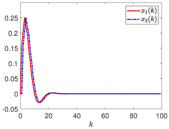
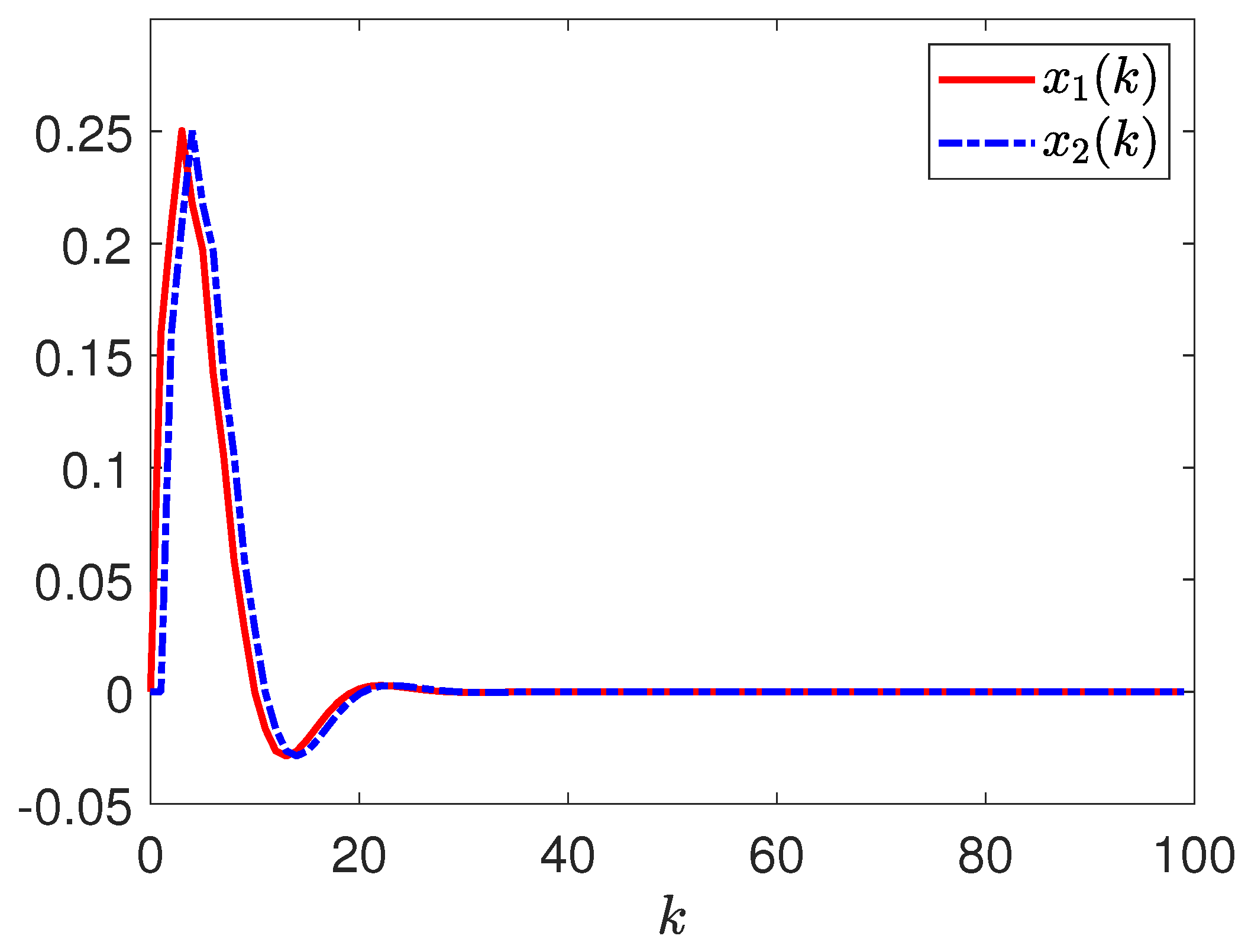
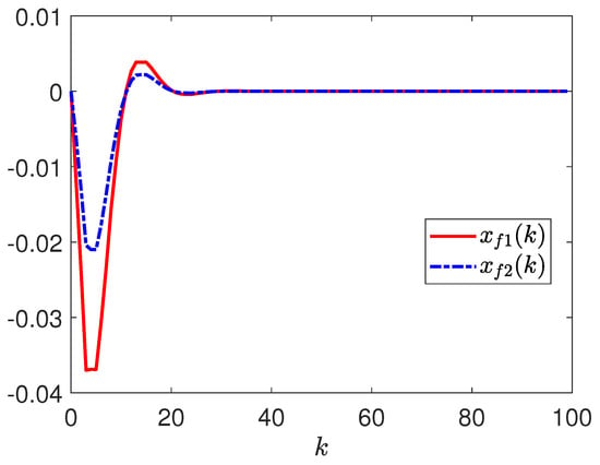
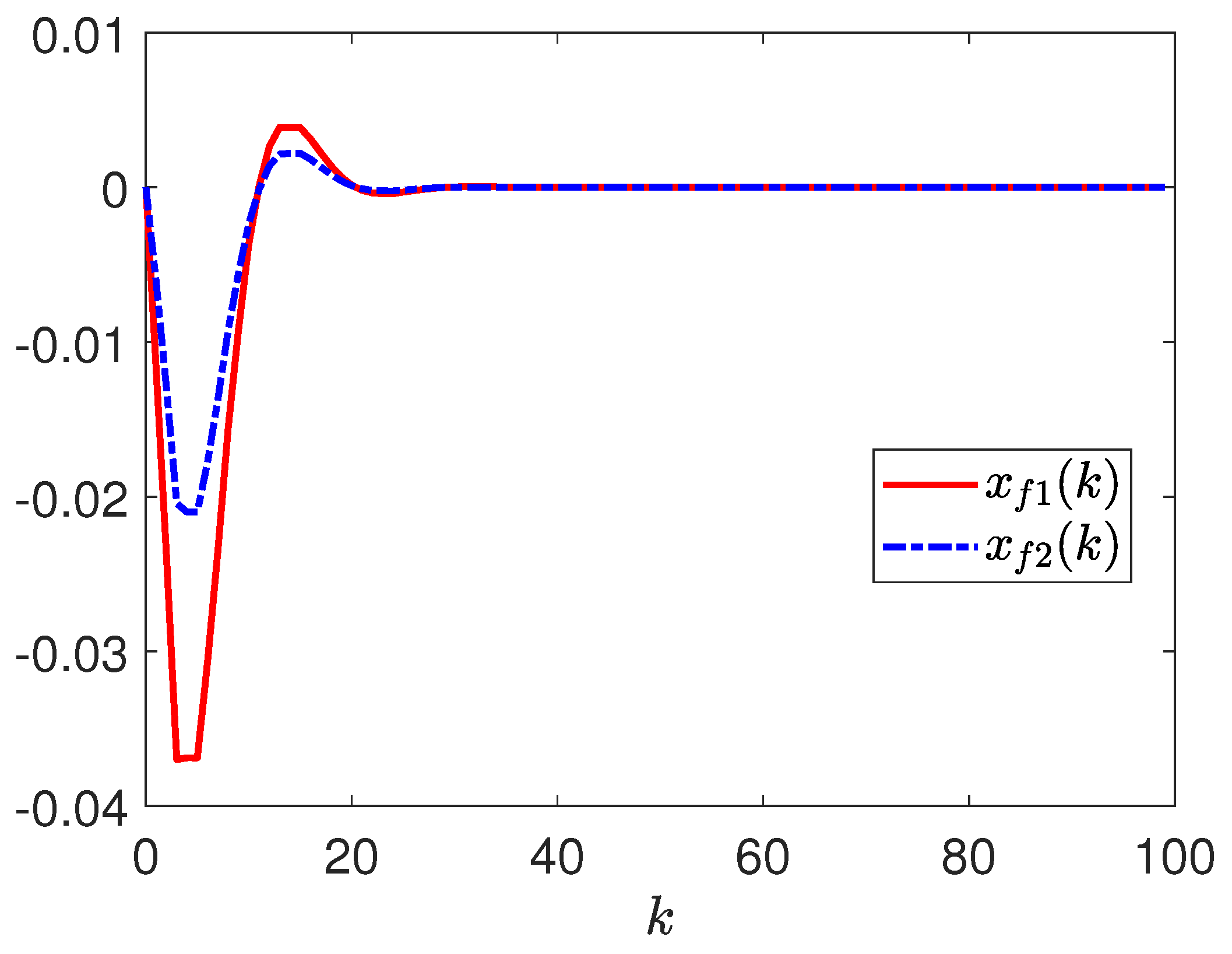
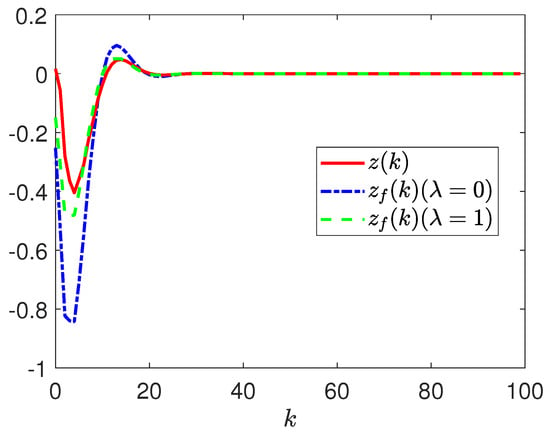
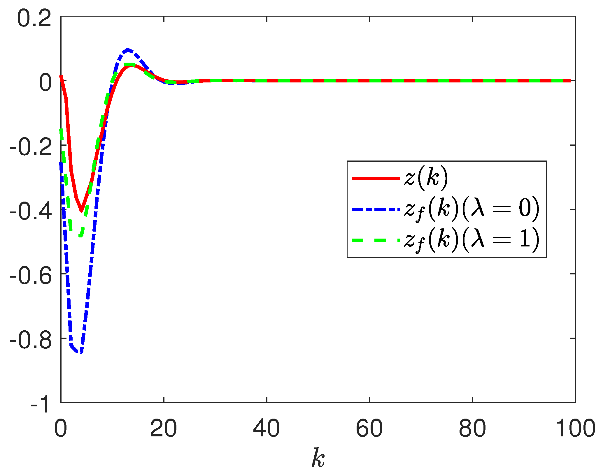
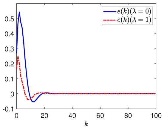
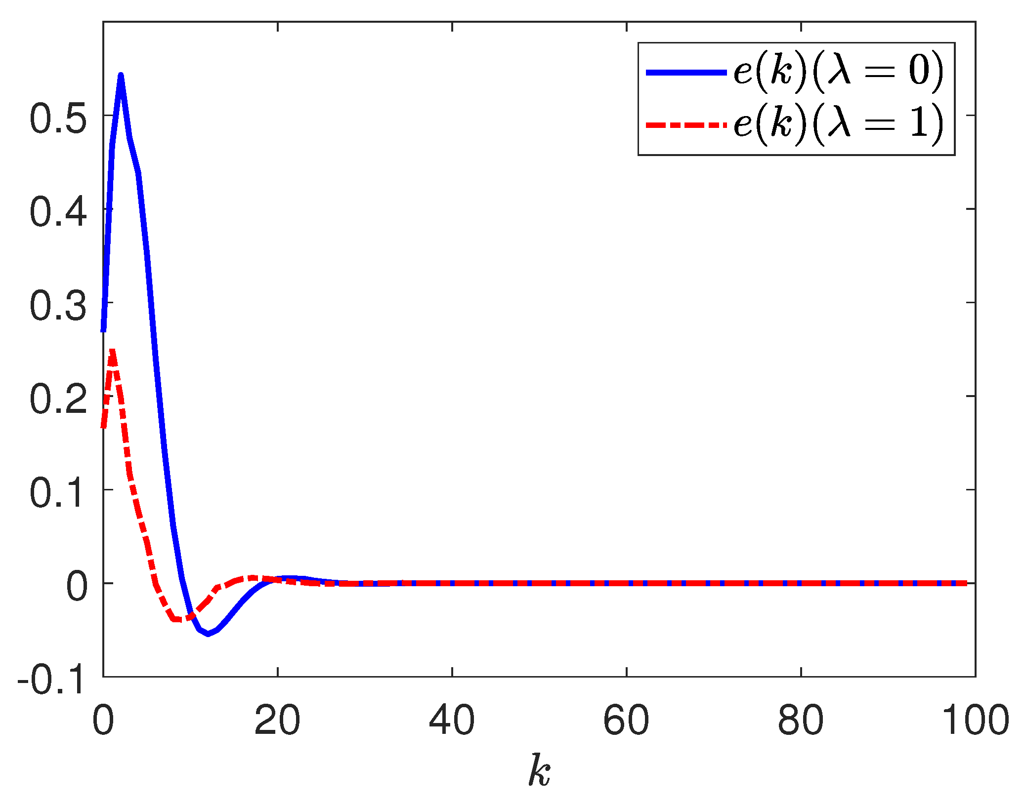
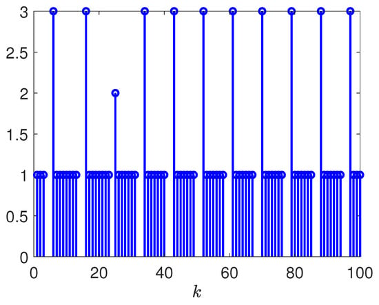
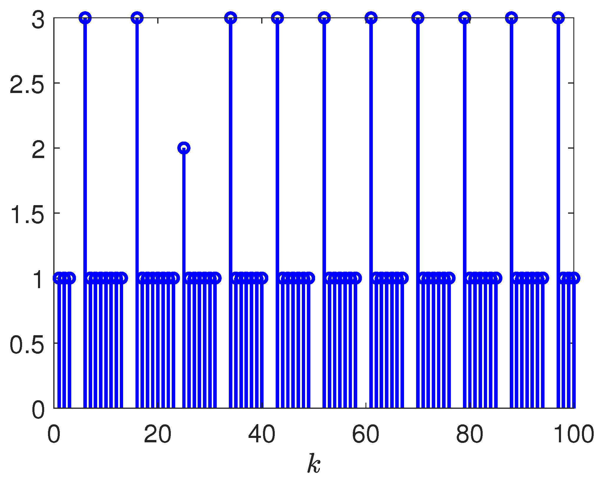
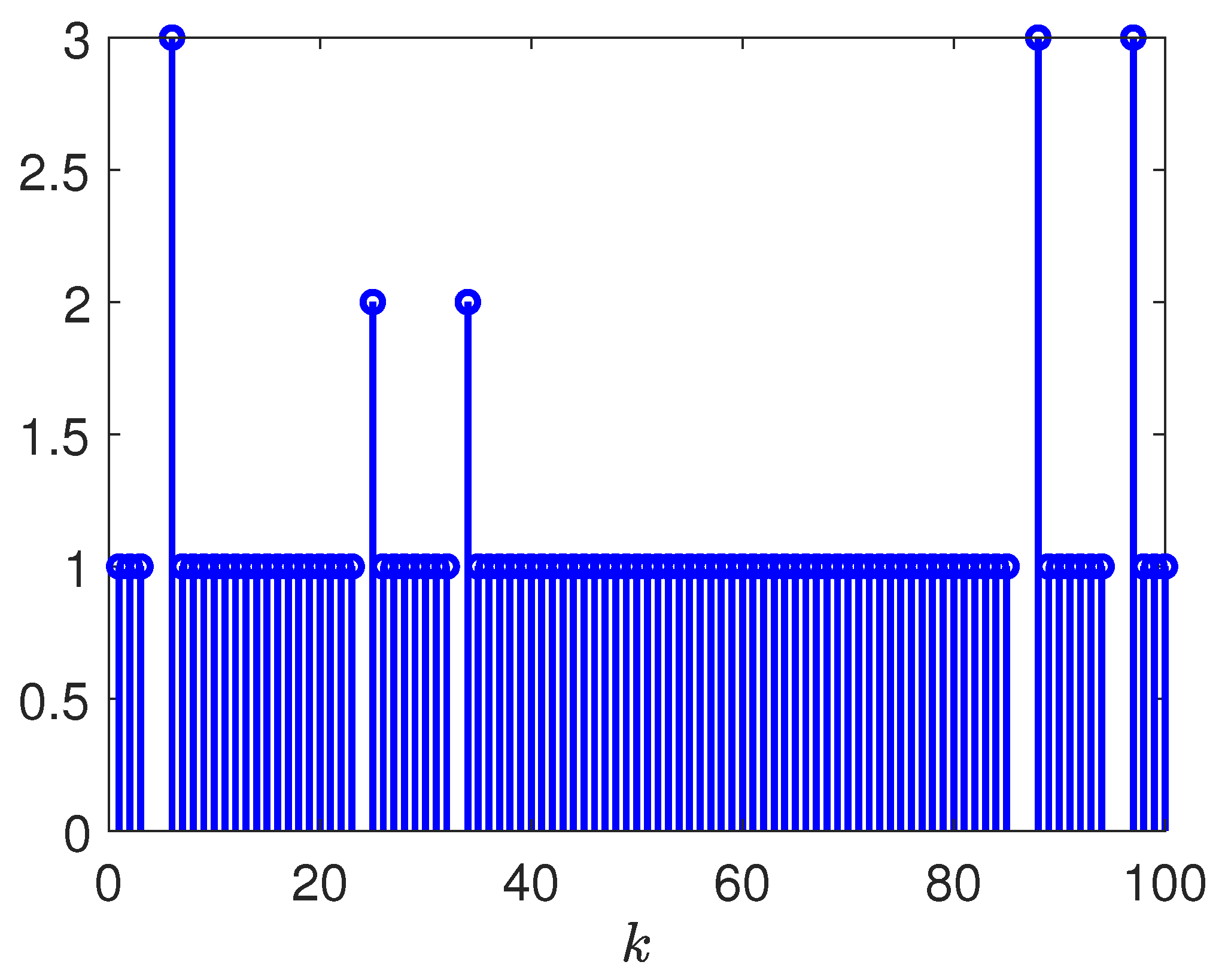
Furthermore, the unknown matrix function, the disturbance input, the initial states of the system and the filter, and the cyber-attack signal are set as ${\Delta }_R=\sin \left(0.1k\right)$, $v\left(k\right)=0.6\sin \left(0.35k\right)e^{-0.25k}$, $x\left(0\right)=x_f\left(0\right)={\left[00\right]}^T$, and $s\left(x\left(k\right)\right)={[-{\left(\tanh \left(0.01x_1\left(k\right)\right)\right)}^T-{\left(\tanh \left(0.01x_2\left(k\right)\right)\right)}^T]}^T$. The responses of the system state $x\left(k\right)$ and the filter state $x_f\left(k\right)$ are depicted in Figure 2 and Figure 3, respectively. Figure 4 presents the responses of the performance output $z\left(k\right)$ and the filter output $z_f\left(k\right)$. Figure 5 depicts the response of the filtering error $e\left(k\right)$. The released intervals of the communication channel from the system to the filter are shown in Figure 6. It can be concluded from the simulation results given in Figure 2, Figure 3 and Figure 4 that, the designed event-triggered robust dissipative filter performs well, as expected.

Figure 2. The response of the system state $x\left(k\right)$.

Figure 3. The response of the filter state $x_f\left(k\right)$.

Figure 4. The responses of the performance output $z\left(k\right)$ and the filter output $z_f\left(k\right)$.

Figure 5. The response of the filtering error $e\left(k\right)$.

Figure 6. The eleased intervals for $\lambda =1$.

To further illustrate that the quantization-dependent event-triggered strategy developed in this paper is more general than the quantization-independent one employed in [15,34], the quantization-independent one employed in [15,34] is also utilized to study the event-triggered robust dissipative filtering problem for this example. By setting $\lambda =0$, the response of the filter output $z_f\left(k\right)$ is depicted in Figure 4, the filtering error $e\left(k\right)$ is shown in Figure 5, and the released intervals of the communication channel from the system to the filter are given in Figure 7.

Figure 7. The released intervals with for $\lambda =0$.

From Figure 6 and Figure 7, we observe that the quantization-dependent event-triggered strategy developed in this paper is triggered only 79 times, fewer than the 92 times of the quantization-independent one employed in [15,34]. Moreover, as shown in Figure 4 and Figure 5, this reduction in data transmissions does not come at the expense of estimation accuracy. Therefore, compared with the quantization-independent event-triggered strategy in [15,34], the developed quantization-dependent one further alleviates the communication burden and conserves communication resources for networked systems with dynamic quantization without compromising estimation accuracy. Additionally, as shown in Figure 6, under the proposed quantization-dependent event-triggered mechanism ($\lambda =1$), the release intervals vary between 1 and 3 sampling periods, and the intervals of 3 sampling periods appear repeatedly over the entire time horizon. This is because the term $\lambda {\theta }^2\left(k\right){\Delta }^2$ in the triggering condition (6) adjusts the triggering threshold adaptively with the quantization error bound: since $\theta \left(k\right)$ is proportional to $\left|y\right(k_q\left)\right|$ as defined in (23), the threshold is enlarged when the quantization is coarse, so that unnecessary transmissions of output variations comparable to the quantization error are avoided. In contrast, for the quantization-independent case ($\lambda =0$), the triggering threshold depends solely on the fixed term $\varphi y^{\mathrm{T}}\left(k_q\right){\mathrm{\Lambda }}_{2}y\left(k_q\right)$, and thus the release interval is almost always 1 sampling period, i.e., the communication channel is occupied at nearly every sampling instant, as shown in Figure 7. Consequently, data transmission is triggered only 79 times under the proposed mechanism, fewer than the 92 times under the quantization-independent one, which indicates that the proposed quantization-dependent event-triggered mechanism achieves a sparser transmission pattern and is thus more desirable for conserving the limited communication resources.

Comparative Explanations: With the developed dissipative filter design strategy, the filtering problem for the Henon mapping system (43) with dynamic quantization, the quantization-dependent event-triggered strategy, and stochastic cyber-attacks can be solved in terms of linear matrix inequalities. Since the dissipative performance considered in this paper covers the ${\mathcal{H}}_{\infty }$ performance and the passive performance as special cases, developed filter design strategy is more general than the ${\mathcal{H}}_{\infty }$ filtering strategies in [26,27,29,30,32,33,39]. Furthermore, the main advantages of the proposed dissipative filtering strategy are summarized as follows.

(1)

In contrast to the existing filtering results, where only the quantization scheme [26,27,28,29] or the event-triggered scheme [35,36,37,38,39,40,41] has been considered, the filtering problem investigated in this paper involves dynamic quantization, event-triggered communication, and stochastic cyber-attacks simultaneously, which is more general and challenging. Specifically, by setting $\lambda =0$, the proposed quantization-dependent event-triggered strategy reduces to the quantization-independent ones in [15,34], and the dynamic quantization scheme adopted herein is more general than its static counterpart in [8,14,18,26,27,30,31]. As shown in Figure 6 and Figure 7, the number of data transmissions under the developed strategy is reduced by approximately 14.13% compared with that under the quantization-independent one, while the estimation accuracy is not compromised, as shown in Figure 4 and Figure 5.

(2)

With the matrix inequality decoupling approach, the design conditions for both full-order and reduced-order filters are derived within a unified framework in terms of linear matrix inequalities, rather than through separate designs as in [28,33]. In contrast to the classic filter design approach widely used in [26,27,28,29,30,33,37], the developed filter design method removes the restrictive assumption on the slack matrix variable, i.e., the requirement that all elements in its second column be identical. Therefore, the developed filter design method is more general than the classic one.

5. Conclusions

In this paper, the robust event-triggered dissipative filtering problem has been investigated for discrete-time networked nonlinear systems under dynamic quantization and stochastic cyber attacks based on T-S fuzzy system theory. To improve the utilization of the limited communication resources, a quantization-dependent event-triggered strategy has been developed, which enables its co-design with the dynamic quantizer to reduce unnecessary data transmissions over the network. Moreover, the effects of stochastic cyber attacks, characterized by the Bernoulli distribution, have also been taken into account. The co-design conditions for the desired dynamic quantizer and the event-triggered filter have been derived in terms of linear matrix inequalities by using the matrix inequality decoupling approach, which guarantee the stochastic stability and the prescribed dissipative performance of the filtering error system. Finally, a practical example has been provided to verify the effectiveness of the proposed filtering scheme. It should be noted that privacy preservation remains a significant challenge for networked systems. Accordingly, extending the proposed robust event-triggered dissipative filtering scheme to nonlinear networked systems with privacy constraints constitutes an interesting topic for future research.

References

- Zhang, X.-M.; Han, Q.-L.; Ge, X.; Ding, D.; Ding, L.; Yue, D.; Peng, C. Networked control systems: A survey of trends and techniques. IEEE/CAA J. Autom. Sin. 2020, 7, 1–17. [Google Scholar] [CrossRef] [Scilit]
- Ren, W.; Xiong, J. H∞ control of linear networked and quantized control systems with communication delays and random packet losses. IEEE Trans. Syst. Man Cybern. Syst. 2022, 52, 3926–3936. [Google Scholar] [CrossRef] [Scilit]
- Yu, K.; Chang, X.-H. Quantized output feedback resilient control of uncertain systems under hybrid cyber attacks. Int. J. Adapt. Control Signal Process. 2022, 36, 2954–2970. [Google Scholar] [CrossRef] [Scilit]
- Yang, H.; Xu, Y.; Zhang, J. Event-driven control for networked control systems with quantization and Markov packet losses. IEEE Trans. Cybern. 2017, 47, 2235–2243. [Google Scholar] [CrossRef] [Scilit] [PubMed]
- Wu, C.; Zhao, X.; Li, C.; Zhao, N. Controller synthesis of asynchronous periodic event-triggered networked control systems subject to quantization effects. IEEE Trans. Signal Inf. Process. Over Netw. 2022, 8, 907–919. [Google Scholar] [CrossRef] [Scilit]
- Zhao, R.; Zuo, Z.; Wang, Y. Event-triggered control for networked switched systems with quantization. IEEE Trans. Syst. Man Cybern. Syst. 2022, 52, 6120–6128. [Google Scholar] [CrossRef] [Scilit]
- Zheng, B.-C.; Yu, X.; Xue, Y. Quantized feedback sliding-mode control: An event-triggered approach. Automatica 2018, 91, 126–135. [Google Scholar] [CrossRef] [Scilit]
- Liu, Y.; Fang, Z.; Park, J.H.; Fang, F. Quantized event-triggered synchronization of discrete-time chaotic neural networks with stochastic deception attack. IEEE Trans. Syst. Man Cybern. Syst. 2023, 53, 4511–4521. [Google Scholar] [CrossRef] [Scilit]
- Liu, J.; Wu, Z.-G.; Yue, D.; Park, J.H. Stabilization of networked control systems with hybrid-driven mechanism and probabilistic cyber attacks. IEEE Trans. Syst. Man Cybern. Syst. 2021, 51, 943–953. [Google Scholar] [CrossRef] [Scilit]
- Zha, L.; Liao, R.; Liu, J.; Xie, X.; Tian, E.; Cao, J. Dynamic event-triggered output feedback control for networked systems subject to multiple cyber attacks. IEEE Trans. Cybern. 2022, 52, 13800–13808. [Google Scholar] [CrossRef] [Scilit] [PubMed]
- Zhou, X.; Liu, S.; Wang, Y.; Zhu, Y. Event-triggered output feedback H∞ control for Markov-type networked control systems. Mathematics 2024, 12, 2666. [Google Scholar] [CrossRef] [Scilit]
- Chang, X.-H.; Liu, X.-M.; Hou, L.-W.; Qi, J.-H. Quantized fuzzy feedback control for electric vehicle lateral dynamics. IEEE Trans. Syst. Man Cybern. Syst. 2024, 54, 2331–2341. [Google Scholar] [CrossRef] [Scilit]
- Zheng, Q.; Xu, S.; Yan, H. Observer-based quantized guaranteed cost control of fuzzy networked control systems with unreliable links and its applications. IEEE Trans. Fuzzy Syst. 2024, 32, 5214–5225. [Google Scholar] [CrossRef] [Scilit]
- Cheng, J.; Wang, Y.; Park, J.H.; Cao, J.; Shi, K. Static output feedback quantized control for fuzzy Markovian switching singularly perturbed systems with deception attacks. IEEE Trans. Fuzzy Syst. 2022, 30, 1036–1047. [Google Scholar] [CrossRef] [Scilit]
- Li, Z.-M.; Chang, X.-H.; Xiong, J. Event-based fuzzy tracking control for nonlinear networked systems subject to dynamic quantization. IEEE Trans. Fuzzy Syst. 2023, 31, 941–954. [Google Scholar] [CrossRef] [Scilit]
- Liu, X.-M.; Chang, X.-H.; Hou, L.-W. Attack-dependent adaptive event-triggered security fuzzy control for nonlinear networked cascade control systems under deception attacks. Mathematics 2024, 12, 3385. [Google Scholar] [CrossRef] [Scilit]
- Liu, X.-M.; Chang, X.-H. Adaptive event-triggered tracking control for nonlinear networked systems with dynamic quantization and deception attacks. Int. J. Robust Nonlinear Control 2024, 34, 8311–8333. [Google Scholar] [CrossRef] [Scilit]
- Liu, J.; Wei, L.; Xie, X.; Tian, E.; Fei, S. Quantized stabilization for T-S fuzzy systems with hybrid-triggered mechanism and stochastic cyber-attacks. IEEE Trans. Fuzzy Syst. 2018, 26, 3820–3834. [Google Scholar] [CrossRef] [Scilit]
- Yang, N.; Fan, X.; Su, H. Dynamic event-triggered delayed impulsive control for stochastic T-S fuzzy complex networks under cyber attacks. J. Frankl. Inst. 2025, 362, 107863. [Google Scholar] [CrossRef] [Scilit]
- Su, X.; Wen, Y.; Shi, P.; Wang, S.; Assawinchaichote, W. Event-triggered fuzzy control for nonlinear systems via sliding mode approach. IEEE Trans. Fuzzy Syst. 2021, 29, 336–344. [Google Scholar] [CrossRef] [Scilit]
- Chen, W.; Fei, Z.; Zhao, X.; Ren, S. Event-triggered asynchronous control for switched T-S fuzzy systems based on looped functionals. J. Frankl. Inst. 2022, 359, 6311–6335. [Google Scholar] [CrossRef] [Scilit]
- Zhu, Y.; Tang, X.; Kang, D.; Zhang, L.; Lv, X.; She, M.; Tan, C. H∞ control of uncertain T-S fuzzy networked control systems with actuator faults under stochastic packet loss-dependent event-triggered schemes. J. Frankl. Inst. 2024, 361, 107119. [Google Scholar] [CrossRef] [Scilit]
- Liu, H.; Hu, J.; Zhang, H.; Zuo, Z. Event-triggered sliding mode control for networked T-S fuzzy delayed systems against random injection attacks. J. Frankl. Inst. 2024, 361, 107333. [Google Scholar] [CrossRef] [Scilit]
- Zhang, J.; Zhao, X.; Zheng, G.; Zhu, F.; Dinh, T.N. On distributed prescribed-time unknown input observers. IEEE Trans. Autom. Control 2025, 70, 4743–4750. [Google Scholar] [CrossRef] [Scilit]
- Zhang, J.; Song, Y.; Zheng, G. Prescribed-time observer for descriptor systems with unknown input. Automatica 2025, 172, 111999. [Google Scholar] [CrossRef] [Scilit]
- Zheng, Q.; Xu, S.; Du, B. H∞ filtering of fuzzy impulsive switched systems with multipath quantizations and packet dropouts via multiple hybrid strategies. IEEE Trans. Fuzzy Syst. 2024, 32, 4178–4191. [Google Scholar] [CrossRef] [Scilit]
- Dong, S.; Su, H.; Shi, P.; Lu, R.; Wu, Z.-G. Filtering for discrete-time switched fuzzy systems with quantization. IEEE Trans. Fuzzy Syst. 2017, 25, 1616–1628. [Google Scholar] [CrossRef] [Scilit]
- Chang, X.-H.; Li, Z.-M.; Park, J.H. Fuzzy generalized H2 filtering for nonlinear discrete-time systems with measurement quantization. IEEE Trans. Syst. Man Cybern. Syst. 2018, 48, 2419–2430. [Google Scholar] [CrossRef] [Scilit]
- Chang, X.-H.; Liu, Y. Robust H∞ filtering for vehicle sideslip angle with quantization and data dropouts. IEEE Trans. Veh. Technol. 2020, 69, 10435–10445. [Google Scholar] [CrossRef] [Scilit]
- Li, W.; Xie, Z.; Wong, P.K.; Hu, Y.; Guo, G.; Zhao, J. Event-triggered asynchronous fuzzy filtering for vehicle sideslip angle estimation with data quantization and dropouts. IEEE Trans. Fuzzy Syst. 2022, 30, 2822–2836. [Google Scholar] [CrossRef] [Scilit]
- Chen, Z.; Zhang, B.; Zhang, Y.; Zhang, Z. Dissipative fuzzy filtering for nonlinear networked systems with limited communication links. IEEE Trans. Syst. Man Cybern. Syst. 2020, 50, 962–971. [Google Scholar] [CrossRef] [Scilit]
- Gu, Y.; Shen, M.; Park, J.H.; Wang, Q.-G.; Yi, Y.; Sun, Y. Dynamic event-triggered H∞ filtering for fuzzy Markov jump systems subject to mismatched quantization. IEEE Trans. Autom. Sci. Eng. 2025, 22, 10639–10649. [Google Scholar] [CrossRef] [Scilit]
- Li, Z.-M.; Xiong, J. Event-triggered fuzzy filtering for nonlinear networked systems with dynamic quantization and stochastic cyber attacks. ISA Trans. 2022, 121, 53–62. [Google Scholar] [CrossRef] [Scilit] [PubMed]
- Li, Z.-M.; Lu, C.; Chang, X.-H.; Xiong, J. Security dissipative fuzzy filtering for networked nonlinear systems with stochastic cyber-attacks. IEEE Trans. Signal Inf. Process. Over Netw. 2025, 11, 1344–1356. [Google Scholar] [CrossRef] [Scilit]
- Xie, X.; Li, S.; Xu, B. Adaptive event-triggered H∞ fuzzy filtering for interval type-2 T-S fuzzy-model-based networked control systems with asynchronously and imperfectly matched membership functions. J. Frankl. Inst. 2019, 356, 11760–11791. [Google Scholar] [CrossRef] [Scilit]
- Su, X.; Wen, Y.; Shi, P.; Lam, H.-K. Event-triggered fuzzy filtering for nonlinear dynamic systems via reduced-order approach. IEEE Trans. Fuzzy Syst. 2019, 27, 1215–1225. [Google Scholar] [CrossRef] [Scilit]
- Liu, Y.; Guo, B.-Z.; Park, J.H.; Lee, S. Event-based reliable dissipative filtering for T-S fuzzy systems with asynchronous constraints. IEEE Trans. Fuzzy Syst. 2018, 26, 2089–2098. [Google Scholar] [CrossRef] [Scilit]
- Zhao, X.; Zhou, S. Intelligent event-triggered filtering for interval type-2 fuzzy singular systems. Asian J. Control 2026, 28, 1258–1274. [Google Scholar] [CrossRef] [Scilit]
- Zhao, N.; Zhao, X.; Zong, G.; Xu, N. Resilient event-triggered filtering for networked switched T-S fuzzy systems under denial-of-service attacks. IEEE Trans. Fuzzy Syst. 2024, 32, 2140–2152. [Google Scholar] [CrossRef] [Scilit]
- Sakthivel, R.; Kwon, O.-M.; Park, M.J.; Sakthivel, R. Event-triggered finite-time dissipative filtering for interval type-2 fuzzy complex dynamical networks with cyber attacks. IEEE Trans. Syst. Man Cybern. Syst. 2023, 53, 3042–3053. [Google Scholar] [CrossRef] [Scilit]
- Xie, X.; Hu, S.; Liu, Y.; Li, Q. Resilient adaptive event-triggered H∞ fuzzy filtering for cyber-physical systems under stochastic-sampling and denial-of-service attacks. IEEE Trans. Fuzzy Syst. 2023, 31, 278–292. [Google Scholar] [CrossRef] [Scilit]
Disclaimer/Publisher’s Note: The statements, opinions and data contained in all publications are solely those of the individual author(s) and contributor(s) and not of MDPI and/or the editor(s). MDPI and/or the editor(s) disclaim responsibility for any injury to people or property resulting from any ideas, methods, instructions or products referred to in the content. |
© 2026 by the authors. Licensee MDPI, Basel, Switzerland. This article is an open access article distributed under the terms and conditions of the Creative Commons Attribution (CC BY) license.