


Abstract
Localizing an underwater acoustic source with a single hydrophone eliminates the cost, synchronization, and deployment burdens of multi-sensor arrays, but the absence of spatial sampling renders the inverse problem underdetermined: positional information must be recovered from the structure that propagation, motion, and vector sensing imprint on a single time series. This review organizes the field along four dimensions. First, the estimation tasks—direction finding, ranging, depth estimation, and tracking—are formalized. Second, the measurement models that generate exploitable structure are derived in a unified notation, covering multipath delays, modal dispersion and waveguide-invariant striations, Doppler and synthetic-aperture effects, and pressure–particle-velocity vector observables. Third, the inference paradigms that map these measurements to position estimates are reviewed, spanning model-based matching, closed-form geometric inversion, Bayesian filtering and batch inversion, and data-driven learning. Fourth, reported accuracies, computational costs, environmental sensitivities, and prior-knowledge requirements are compared across method families. The evidence indicates that relative range errors of 1–10% are routinely reported, whereas depth estimation is structurally harder and remains the principal accuracy bottleneck. Environmental mismatch, multipath resolvability, multi-source interference, and the out-of-distribution generalization of learned models constitute the main open challenges; physics–learning hybridization, uncertainty-aware estimation, vector-hydrophone designs, and joint localization–environment inversion are identified as promising directions.
MSC:
76Q05
1. Introduction
Covering approximately 71% of the Earth’s surface, the ocean is central to economic development, scientific research, and maritime security, and its exploration has attracted sustained international attention [1]. The principal modalities for ocean exploration are underwater acoustics, optics, and electromagnetics. Light and electromagnetic waves are strongly absorbed and attenuated in seawater, which severely limits their effective detection range [2]. Underwater acoustic techniques, which exploit the long-range propagation of sound in the ocean, therefore provide the primary means of remote underwater sensing.
Acoustic source localization, as a core technique of underwater detection, is applied in military operations [3], marine engineering [4], marine archaeology [5], and underwater robotics [6]. Conventional underwater source localization relies predominantly on multi-baseline systems, including long baseline, short baseline, and ultra-short baseline systems, which are limited by high cost, stringent synchronization requirements, and difficult deployment [7]. Single-receiver localization instead estimates the source position from the signal of one receiver only; it offers a simple system configuration, low cost, and ease of deployment, and it has become an active research topic in underwater acoustics [8].
This paper focuses on source localization with a single receiver, where the term “single receiver” denotes a solitary hydrophone unit without spatial sampling capability (i.e., it cannot form an array to acquire spatial information). The central question is therefore how to exploit information that is detrimental to conventional localization—such as multipath propagation and the relative motion between source and receiver—to accomplish localization in the absence of spatial information. This review covers not only methods based on a single scalar (pressure) hydrophone but also methods relying on a vector hydrophone, which measures the acoustic pressure and the particle-velocity vector (or acceleration vector) at the same point in the sound field. A single vector hydrophone can thus also be regarded as a “single receiver”, namely, “a collocated multi-channel sensor of vanishing aperture”, and it has been an active research topic in underwater vector acoustics since the 1990s [9].
As summarized in Table 1, this review provides a focused treatment of single-hydrophone source localization, with particular emphasis on acoustic vector hydrophone (AVH) technology. Existing surveys address network localization algorithms [10], taxonomic frameworks [11], MEMS AVS hardware [12], or underwater positioning and tracking at the system level [13]; they predominantly consider multi-node systems and provide limited discussion of reverberation and multipath impairments, and none offers a unified treatment of single-hydrophone localization spanning DOA estimation, ranging, and target tracking. The present review addresses this gap by integrating these signal processing dimensions into a dedicated review of single-hydrophone scalar- and vector-sensor localization.
Table 1.
Comprehensive comparison of acoustic source localization surveys.
Consequently, this study defines single-hydrophone localization in the following manner: By leveraging the signal data received by a single receiving unit, and in the absence of spatial information at the receiver, compensation is implemented through the comprehensive utilization of time-domain, spatial, frequency-domain information, as well as the prior knowledge of the sound source. Subsequently, in conjunction with the physical model of underwater acoustic propagation (such as ray theory or normal-mode model) or data-driven model (such as machine learning/deep learning), the formidable task of underwater sound source localization is tackled. Through an in-depth exploration of the fundamental principle of single-hydrophone localization and a systematic analysis of the scenarios and challenges addressed by existing algorithms, this review endeavors to put forward and address the following core research questions (RQs), aiming to assist readers in gaining a deeper understanding of the current state and development of this field:
- RQ1.
- What are the fundamental mathematical and physical models for single-hydrophone signal observation within an underwater environment? What are the associated modeling paradigms?
- RQ2.
- In the literature, what algorithmic principles and signal processing techniques have been put forward to address the single-hydrophone localization problem? How do they vary with respect to assumptions regarding target signals, channel models, localization parameters, and solution strategies?
- RQ3.
- How do different single-hydrophone localization methods compare in terms of key performance indicators? What trade-offs become evident from these comparisons?
- RQ4.
- What are the primary technical and theoretical challenges confronting current single-hydrophone localization systems? Which emerging directions are anticipated to achieve breakthroughs in the future?
To address the above research questions systematically, this review is organized through a rigorous literature retrieval and screening process, a thorough review of the underlying theories, and in-depth analysis of localization principles.
Literature Retrieval and Screening Methodology: The literature covered by this review was retrieved from Web of Science, Scopus, IEEE Xplore, and Google Scholar using combinations of the keywords “single hydrophone”, “single receiver”, “single vector sensor”, “underwater acoustic source localization”, “passive ranging”, “multipath time delay”, “modal dispersion”, “warping transform”, “waveguide invariant”, “Doppler”, “synthetic aperture”, and “machine learning localization”. The search covered publications from 1990 to 2025, including journal articles, conference proceedings, and doctoral dissertations. A study was included if (i) localization (DOA, range, depth, position, or tracking) is performed with a single receiving unit, or the method is directly transferable to that setting; (ii) the underlying signal processing principle is described in sufficient detail; and (iii) for the performance comparison of Dimension IV, quantitative results are reported. Studies relying on spatially distributed multi-element arrays were excluded unless they provide the theoretical basis of a single-receiver method. The reference lists of all retained papers were cross-checked to identify additional relevant works.
The remainder of this review is organized as follows: Section 2 presents the propagation physics and the mathematical model of the signal received by a single underwater receiver. Section 3, the core section, presents the basic principles of single-receiver underwater localization and proposes a four-dimension classification framework: Dimension I (Section 3.1) organizes methods by estimation task; Dimension II (Section 3.2) reviews the algorithm families grouped by physical principle; Dimension III (Section 3.3) treats statistical inference and data-driven paradigms; and Dimension IV (Section 3.4) compares performance metrics and trade-offs. Section 4 analyzes the key challenges and future prospects in single-hydrophone localization and potential future research directions. Section 5 concludes the review.
The four dimensions are deliberately chosen as orthogonal facets of any localization method rather than as a single hierarchical taxonomy, and they answer four successive questions that a designer faces: what is to be estimated (Dimension I: ranging, depth, direction finding, or tracking, each with distinct observability conditions); where the positional information comes from (Dimension II: the physical mechanism—multipath, modal dispersion, motion, or vector observables—that imprints position on a single time series); how the estimate is computed (Dimension III: model-based matching, closed-form inversion, Bayesian filtering, or data-driven learning); and how well the result performs in practice (Dimension IV: accuracy, cost, robustness, and prior-knowledge requirements). Read in sequence, the dimensions form the pipeline task → observable → estimator → performance, so that every method occupies a point in a four-dimensional design space. This contrasts with reviews organized solely by algorithm category, where the physical origin of the information and the inference machinery are entangled: separating the two exposes cross-family transfer (e.g., the same multipath-delay observable can feed a geometric solver, a matched-field grid search, or a neural regressor) and reveals unexplored combinations, which is precisely where the open directions of Section 4 arise.
2. Propagation and Measurement Models
For a single hydrophone to accomplish localization, fundamentally, the characteristics of the received signal must be spatially resolvable. This enables the indirect inference of the sound source’s position. It is therefore necessary to analyze the complete chain from source emission, through propagation, to reception by the hydrophone. Two modeling levels are distinguished in this section: the propagation model and the reception model. The propagation model describes the physical field generated by the source in the ocean acoustic channel, whereas the observation model describes how the hydrophone converts these physical fields into measurable signals. This section concludes with the design considerations for the received-signal model in single-hydrophone localization. For quick reference, the principal mathematical symbols used throughout this review are summarized in Appendix A.
2.1. Propagation Models
Underwater localization fundamentally builds upon wave acoustics. Compared with air, underwater sound propagation is strongly influenced by absorption, boundary reflections, refraction due to sound-speed variations, and scattering from medium inhomogeneities. As a result, the received field is often characterized by multipath propagation, which simultaneously complicates and enables localization with a single receiver.
Let denote the spatial position vector and t the time variable. The primary physical quantities describing the acoustic field are the sound pressure and the particle velocity vector . In vector hydrophone systems, particle velocity is particularly important since it encodes the wave’s propagation direction. Under the assumption of small acoustic perturbations, these quantities are governed by the linear momentum, continuity, and state equations in a homogeneous and isotropic fluid:
where is the medium equilibrium density, is the sound speed profile, and ∇ denotes the spatial gradient operator. In the frequency domain, particle velocity relates to the pressure gradient as
The frequency-domain form Equation (4) enables in-depth analysis of harmonic responses, impedance relationships, phase and amplitude characteristics that are contingent upon frequency. Importantly, in the plane-wave (far-field) limit, with wave number , is the angular frequency so
where is the characteristic impedance and is the propagation unit vector. This asymptotic Equation (5) implies a near-linear amplitude scaling between pressure and particle velocity and co-phasing of the two fields in the far field that contains directional information essential for bearing estimation. [9]. However, in near-field regions, and whenever strong scattering, diffraction, or boundary-induced evanescent components are present, pressure and velocity can exhibit substantial phase offsets and nontrivial directional structure [19].
This relationship indicates that, once the pressure field is solved, both pressure and velocity fields are available. Substituting these into Equations (1)–(3) yields the classical linear acoustic wave equation:
with denoting the Laplacian operator. This equation describes the evolution of the acoustic pressure field in space and time, and it serves as the starting point for a variety of propagation models. A variety of modeling approaches have been developed to solve the wave equation under realistic ocean conditions. The majority of fundamental theories addressing underwater acoustic propagation problems-including ray theory, normal-mode theory, parabolic equation theory, etc., are derived from wave fluctuation equations. These theoretical frameworks provide distinct approaches to modeling sound propagation in underwater environments, each with specific advantages and limitations.
2.1.1. Ray Theory
An approximate approach derived from geometric optics is employed to depict the propagation of waves. Nevertheless, this method does not yield a complete solution; instead, it offers an effective approximation under high-frequency circumstances. This theory conceptualizes the transmission of sound energy in the form of rays. A ray is defined as the normal to the wavefront, which indicates the direction of propagation. The superposition of these ray clusters forms the observable sound field environment. The ray model describes, in a highly intuitive manner, the propagation of sound energy within the medium. Its solution to the wave equation can be expressed as
where , termed transport function, governs the slow spatial and spectral variation of the field along a ray tube. termed the phase function, determines ray trajectories by expressing path length as a function of path endpoints. The eikonal relation is written as . Surfaces of constant phase are referred to as wavefronts, and the trajectories orthogonal to those surfaces are called sound rays. When such a trajectory links the source and a receiver, it is termed a characteristic sound ray; each characteristic ray uniquely determines a propagation delay and a geometric spreading factor that govern its contribution to the measurement field.
Ray theory is widely used in localization because it provides an intuitive and computationally efficient description of propagation delays and arrival angles. It is an asymptotic, high-frequency approximation and therefore becomes unreliable when diffraction, strong modal interference, or caustics dominate. A common empirical rule of thumb is
where f is frequency, is the water depth and c is the sound speed; this condition implies the wavelength is much smaller than the water depth, which justifies the ray approximation.
2.1.2. Normal-Mode Theory
In contrast to ray theory, the normal-mode model provides an exact solution of the wave equation for a range-dependent waveguide by expanding the acoustic pressure field into discrete eigenfunctions of the medium. This approach is particularly well suited to low-frequency and long-range scenarios, where the number of propagating modes is small, and each mode corresponds to a physically interpretable propagation path.
The solution to the wave Equation (6) can be decomposed into the product of a depth function and a radial propagation function, yielding the modal expansion form in cylindrical coordinates :
where are the depth-dependent eigenfunctions that satisfy the vertical boundary conditions, and are the horizontal mode amplitudes governing radial dependence.
In the normal-mode model, each mode can be construed as a traveling wave in the range direction, giving rise to a zero-order Bessel equation. The solution thereof can be formulated as a zero-order Hankel function. In the depth direction, it manifests as a standing wave, thereby formulating an eigenvalue problem within the normal-mode equation, and its solution is the Green function. The normal-mode theory offers an effective approach for characterizing the sound field via the superposition of discrete waveguide modes in sound propagation computations. The solution of the wave equation is presented in the form of the expansion and superposition of normal modes, and the eigenvalues and eigenfunctions are derived by solving the normal-mode equation that adheres to specific boundary conditions.
When the frequency of the acoustic signal is relatively low or the ocean depth is relatively shallow, the order of the normal modes capable of propagating within the channel is also reduced. Consequently, for low-frequency sound fields in shallow water, the normal-mode model offers high accuracy at low computational cost. The normal-mode model is able to derive a set of vibration modes, and the “frequency” of the vibration can yield the horizontal wave number that is closely associated with mode propagation. For a waveguide featuring pressure-release interfaces at the sea surface and rigid bottom, the cut-off frequency of the n-th mode is
2.1.3. Parabolic Equation and Full-Wave Numerical Theory
High-fidelity wave-equation models—notably parabolic-equation (PE) formulations and full-wave numerical solvers (finite-difference time-domain, finite-element, boundary-element)—retain wave phenomena omitted by geometric acoustics and simple modal representations. These phenomena include diffraction around obstacles, complex scattering from range-dependent structures, and precise near-field phase and reactive effects. PE implementations exploit a small-angle approximation to efficiently simulate long-range, depth-varying, broadband propagation; full-wave solvers dispense with angular restrictions and therefore can reproduce arbitrary angular spectra and near-field interactions, albeit at substantially higher computational cost.
From a signal-processing perspective, PE and full-wave models play three principal and complementary roles. First, they generate realistic synthetic datasets for training and benchmarking data-driven algorithms, a capability that is vital when in situ labeled data are scarce. Second, they provide accurate forward operators for physics-informed inversion frameworks—enabling waveform-level maximum-likelihood or Bayesian estimation that fits observed waveforms rather than relying on simplified arrival-time metrics. Third, they support rigorous uncertainty analysis by quantifying how errors in environmental parameters (e.g., sound-speed profile, bathymetry, seabed properties) propagate into localization bias and variance. For single-hydrophone localization tasks that demand waveform fidelity—matched-field processing, waveform-based Bayesian inversion, or end-to-end supervised learning—PE/full-wave models are often necessary despite their computational expense. Practically, a common workflow is to use PE/full-wave simulations offline to develop and validate algorithms, then deploy surrogate or reduced-order models (calibrated to the high-fidelity outputs) in real-time or resource-limited operational contexts.
2.2. Measurement Models
Building upon the propagation framework, the measurement model establishes a mathematical linkage between acoustic wave transmission and the observables accessible to a single hydrophone. In contrast to array-based localization, which leverages spatial diversity to directly derive directional information, single-receiver scenarios rely on extracting indirect observables from the received waveform. The primary challenge in single-hydrophone localization lies in deriving sufficient spatial information from a solitary measurement point, which is achieved by exploiting the acoustic field structure governed by source characteristics and the propagation environment.
Depending on the physical mechanisms employed, various measurement models can be constructed, each underpinning a distinct class of localization algorithms. For the received acoustic pressure signal , the fundamental measurement model is typically expressed as the convolution of the source signal with the channel impulse response , where the impulse response is a function of unknown parameters , which encompasses both environmental and geometrical parameters, such as range, depth, velocity, environmental conditions, and boundary properties, etc.
where is additive noise and ∗ denotes convolution in time. The specific form of and the subsequent processing strategies define the different localization methodologies. In the context of vector velocity signals, the measurement model is further extended to incorporate joint information from acoustic pressure and the particle velocity vector. This emphasizes that the channel impulse response should reflect the correlated multiplicative relationship between the pressure component and the vector form of particle velocity (or acoustic particle velocity flow). Specifically, the extended channel impulse response function can be represented in vector form as .
The measurement model formalizes the relationship between the transmitted source signal and the waveform recorded at a single hydrophone. Depending on the physical propagation mechanisms, receiver configuration, and inference paradigm, several distinct formulations can be established. In what follows, we summarize the major classes of measurement models relevant to single hydrophone localization.
2.2.1. Measurement Model for a Single Scalar Hydrophone
The propagation model based on ray theory, as presented in Section 2.1.1, shows that acoustic rays propagating along different paths exhibit distinct arrival times (time delays) due to differences in path lengths and the number of boundary reflections. This phenomenon has directly motivated the development of multipath arrival-based models. In contrast, the propagation model rooted in normal-mode theory, detailed in Section 2.1.2, reveals that the acoustic field is formed by the superposition of a discrete set of globally supported vibrational modes within the waveguide. Each mode exhibits unique dispersion characteristics—specifically, frequency-dependent phase and group velocities. As a result, the total acoustic pressure recorded at a single hydrophone constitutes a scalar measurement.
Multipath Arrival Based Received Signal Model
In conventional multi-sensor localization systems, multipath propagation is typically regarded as a source of interference, and significant efforts are often dedicated to its suppression or mitigation. In stark contrast, for the single-hydrophone localization problem, the multipath structure is not a detrimental artifact but rather forms a crucial environmental fingerprint. The distinct time delays, attenuation factors, and phase shifts associated with the various propagation paths inherently encode spatial information about the source and the environment. These characteristics provide exploitable localization cues that can be leveraged by methods based on time-delay estimation, model inversion, or statistical learning. Consequently, for the single-sensor localization problem, the appropriate characterization and utilization of the multipath structure is pivotal for enhancing localization accuracy and robustness.
When the acoustic wavelength is significantly smaller than the characteristic environmental scales, such as water depth or the scale of sound speed gradients, the ray propagation approximation provides a valid model. Under this assumption, effects like diffraction and inter-mode coupling can often be neglected. The received signal can then be modeled as a superposition of a finite number of distinct arrivals, resulting from specular reflections from boundaries (surface and bottom) and refraction due to the sound speed profile. The received signal is thus a sum of time-delayed, amplitude-scaled, and phase-shifted replicas of the original source signal. The channel impulse response introduced in Equation (11) can be specifically expressed under this ray-based, multipath model as follows:
where and are the complex amplitude and time delay of the m-th path, respectively, which are dependent on the source and receiver location parameters . The integer M denotes the total number of significant multipath components considered in the model. The time differences between these various paths constitute key observables. These measured Time Differences of Arrival (TDOAs) provide geometric constraints that can be matched against a ray-theoretic propagation model to estimate the source position.
Modal Interference Received Signal Model
Compared to the ray-geometric perspective, normal-mode theory permits decomposition of the acoustic field into physically interpretable components. In shallow water at low frequencies, the field is often well represented by a modest number of normal modes. For a pulsed transmission, each mode’s group velocity depends on modal order and frequency; consequently, modal dispersion occurs at the receiver. From the normal-mode viewpoint, modal dispersion illustrates that—even within the same path class—modal components propagate with different group velocities, leading to waveform distortion and temporal broadening at the hydrophone.
A more detailed description of the channel in a stratified ocean waveguide is obtained via modal decomposition. In this representation, the received field is expressed as a superposition of normal modes, each characterized by a depth-dependent eigenfunction and a mode-specific group delay. The channel impulse response in Equation (11) can be idealized as
where N denotes the number of propagating modes, is the modal excitation coefficient determined by , is the depth-dependent eigenfunction of mode n at both source depth and receiver depth , and is the modal group delay of the n-th mode. This formulation explicitly captures inter-modal dispersion through the mode-dependent group delays , which vary with both modal order and frequency. The frequency-domain representation follows directly through Fourier transformation:
where modal superposition produces constructive and destructive interference across frequency and range. These modal interference patterns manifest as characteristic striations in the time–frequency and frequency–range domains. The fringe spacing is governed by an approximate invariant relationship. For the interference between two modes, the spacing satisfies
where and are the frequency and range spacings of interference fringes, and is the waveguide invariant. The invariant , defined as for phase speed and group speed , encapsulates the average modal dispersion properties of the environment and is relatively insensitive to moderate environmental perturbations. This scalar characterization of the interference structure was introduced by Chuprov [20]—in whose honor the parameter is often called the “Chuprov invariant”—and its theory was subsequently formalized for layered waveguides by Grachev [21].
Thus, the modal-dispersion model provides a rigorous physical description of the underwater acoustic channel. It explains that the received signal is a superposition of normal modes, each traveling at a distinct group velocity, which leads to modal dispersion in the time domain. In the frequency domain, the interference between these modes generates a structured striation pattern, the geometry of which is governed by the waveguide invariant. This synthesis of modal physics in the time domain and interference geometry in the observation domain constitutes a compact and powerful measurement model.
2.2.2. Measurement Model for a Single Vector Hydrophone
When the receiver is a collocated vector hydrophone, under a far-field plane-wave approximation, the measurement reduces to the rank-1 structure both acoustic pressure and particle velocity components are measured. The multi-channel particle-velocity measurement is modeled as the convolution of the source waveform with a vector impulse response
where the additive noise term is compactly written as representing pressure and three velocity-axis hydrophone channel noise. It is usually assumed that the four channels are mutually uncorrelated. denotes the pressure impulse response in Equations (12) and (13) and denotes the particle-velocity impulse responses along the three sensor axes. In the homogeneous medium and narrowband limit the velocity impulse-response vector is collinear with defined as Equation (5) and proportional in amplitude to the pressure response by the plane-wave acoustic impedance factor ,
where is the unit propagation vector in Cartesian coordinates with elevation from axis and azimuth in the -plane from axis.
Multipath perspective: Each propagation path m is associated with a distinct propagation direction . Hence, in the multipath sum,
The scalar pressure contributions from different paths combine without directional labels, whereas the velocity contributions carry explicit, path-dependent direction vectors . This per-path directional diversity provides immediate cues for direction-of-arrival (DOA) estimation and assists in discriminating overlapping arrivals that may be ambiguous in pressure-only observations.
Modal perspective: In modal representation, different modes contribute with distinct modal velocity shapes and mode-dependent pressure–velocity transfer characteristics. Even where pressure spectra of two modes overlap, their velocity modal shapes (both orientation and depth dependence) can differ markedly, producing complementary information useful for resolving modal interference and for constraining inverse problems (e.g., source localization) that are ill-posed when using pressure alone.
In a waveguide the pressure and velocity fields are naturally expanded in normal modes like (14):
where and are the pressure and particle-velocity modal shape functions, respectively, and are the mode wave-numbers. The modal coefficients and are connected through mode-dependent impedances (or admittances) and boundary conditions; consequently, the relative amplitude and phase between pressure and velocity are generally frequency and depth dependent.
The vector modal shapes are typically not collinear with the pressure modal shapes and may exhibit distinct depth and phase profiles. Thus, modal dispersion induces frequency-dependent pressure–velocity relations and modal interference features in both scalar and vector channels.
2.2.3. Motion-Based Model
In the motion-based (synthetic-aperture) reception setting with a spatially fixed source, the measurement model is governed primarily by the receiver kinematics and the induced propagation delays. Let denote the known receiver trajectory and the fixed source location; the one-way propagation delay at time t is
is a slowly varying amplitude factor that models geometric spreading and attenuation, the continuous-time received signal is written as
The salient characteristics of this motion model are the receiver trajectory determines the effective synthetic aperture and thus the spatial sampling geometry; Meanwhile, variation in delays across successive snapshots provides virtual aperture information, enabling localization even when multipath or modal structure is weak. This forms the basis of synthetic aperture processing and sequential triangulation approaches.
In practice the two paradigms are complementary: physics-based statistical models supply interpretable likelihoods and rigorous uncertainty statements, while data-driven models offer computational efficiency and robustness to unmodeled complexity. A pragmatic strategy is to employ physics-based forward simulators to generate diverse training sets for learned models, and to retain Bayesian or ensemble techniques to quantify prediction confidence in deployment.
2.3. Summary of Propagation and Measurement Models
In summary, this chapter has reviewed two essential layers of modeling for single-hydrophone localization. The first part introduced propagation models, including ray theory, normal-mode theory, parabolic equation methods, and full-wave numerical formulations, which provide rigorous physical descriptions of acoustic energy transmission in the ocean environment. These frameworks establish how sound propagates through range-dependent, stratified, and potentially uncertain media, thereby underpinning all subsequent measurement formulations.
Building on this foundation, the second part focused on measurement models, which map the physical propagation process to the actual hydrophone observations. Multipath and mode-based formulations emphasize deterministic structures of the waveguide response, while motion-based and vector-hydrophone models enrich the available observables. In contrast, statistical and data-driven approaches abstract the input–output mapping into probabilistic or learned representations, offering modeling flexibility at the expense of explicit interpretability.
Together, propagation and measurement models provide a comprehensive basis for localization research: the former defines the underlying physics, and the latter structures the observations available for estimation. The following chapter therefore shifts attention from physical and measurement modeling toward algorithmic methodologies, examining how different estimation strategies—ranging from matched-field processing and Bayesian inference to machine learning and hybrid approaches—exploit these models for robust source localization.
3. Algorithmic Approaches for Single-Hydrophone Localization: Principles, Assumptions, and Performance
The fundamental challenge of source localization with a single hydrophone stems from the intrinsic loss of spatial diversity. Unlike hydrophone arrays, which leverage phase differences across spatially separated sensors to resolve source location, a single sensor must extract all locational information from the temporal and spectral structure of the received signal. This necessitates sophisticated signal processing techniques that exploit the interplay between the source emission, the underwater channel’s physical characteristics, and the geometry of the propagation paths.
This section reviews the algorithmic principles devised to address this challenge, dissecting the underlying assumptions, operational mechanisms, and limitations of each major method class. This analysis addresses RQ2 by cataloging the signal processing techniques found in the literature; by comparing their accuracy, complexity, robustness, and prior-knowledge requirements, it further provides a comparative framework for identifying trade-offs, thereby addressing RQ3.
The chapter is organized as follows. Section 3.1 introduces a task-oriented classification that organizes single-receiver localization problems according to their estimation objectives. Section 3.2 then presents a taxonomy that categorizes existing methods by their core signal processing principles, followed by a detailed exposition of each algorithm family. Section 3.3 treats the statistical inference and data-driven paradigms, including Bayesian estimation and machine-learning approaches. Finally, Section 3.4 presents a comprehensive performance comparison and discusses the trade-offs among these method families.
3.1. Dimension I: Task-Oriented Classification of Single-Receiver Localization
Single-receiver localization problems can be systematically categorized according to the specific estimation objectives. Different tasks require distinct levels of spatial information recovery and impose different observability conditions on the received acoustic field.
From a task-oriented perspective, existing studies can be broadly divided into four categories: direction-of-arrival (DOA) estimation, range and depth estimation, 2D/3D localization, and target tracking.
3.1.1. Task 1: Direction-of-Arrival Estimation
Direction-of-arrival estimation aims to determine the bearing of the acoustic source relative to the receiver. For a single vector hydrophone, DOA estimation exploits both the acoustic pressure and particle velocity components, enabling intrinsic directional sensitivity without requiring spatial aperture.
Vector sensors provide two major advantages: 1. The ability to directly estimate the acoustic intensity vector. 2. Enhanced performance under low SNR and coherent multipath environments.Typical approaches include intensity-based methods, subspace techniques adapted to vector measurements, and statistical beamforming formulations. DOA estimation provides angular information only and does not inherently resolve range ambiguity.
3.1.2. Task 2: Range Estimation (Or Depth Estimation)
Range estimation extends beyond angular recovery and aims to determine the source-receiver separation. This may include depth, horizontal or slant distance estimation.
In single-receiver scenarios, range estimation typically relies on additional structural information, such as multipath arrival time differences, modal interference patterns in waveguides, motion-induced geometric diversity. Unlike DOA estimation, range recovery requires exploiting propagation structure rather than purely local field directionality.
3.1.3. Task 3: 2D and 3D Localization
Full localization refers to recovering the complete spatial coordinates of the source, either in a two-dimensional horizontal plane, or in three-dimensional space (range, depth, and azimuth). This task requires jointly estimating angular and distance parameters and is generally formulated as a nonlinear inverse problem.
For single-receiver systems, full localization is achievable only when sufficient independent constraints are available, such as multiple resolvable multipath arrivals, environmental modal structure, receiver motion over time. The feasibility of full localization is fundamentally tied to observability and identifiability conditions.
3.1.4. Task 4: Target Tracking
Target tracking extends localization into the temporal domain by estimating a time-evolving state sequence. Instead of solving independent localization problems at each time instant, tracking methods incorporate dynamic models, such as constant velocity or acceleration motion models, doppler-based kinematic constraints, bayesian filtering frameworks (e.g., EKF, UKF, particle filters)
Tracking improves robustness and estimation accuracy by exploiting temporal continuity and state-space modeling. In single-receiver configurations, motion—either of the source or the receiver—often plays a critical role in enhancing observability over time.
To further reveal the intrinsic relationship between estimation objectives and methodological paradigms, Table 2 summarizes the major task categories and their corresponding information requirements, typical algorithmic approaches, and observability conditions.
Table 2.
Task-oriented classification of single-receiver localization: estimation targets, required information, typical methods, and observability conditions.
The four task categories reflect increasing levels of spatial information recovery, from angular estimation to full spatio-temporal state reconstruction. While DOA estimation primarily relies on the directional capability of vector sensors, range and full localization require exploiting propagation structure or temporal diversity. Tracking further introduces dynamical constraints that fundamentally alter the observability properties of the problem. This task-oriented classification provides a functional perspective that complements method-based or model-based categorizations.
3.2. Dimension II: Classification of Underwater Acoustic Target Localization Methods Based on Single Hydrophone
The classification of single-hydrophone localization methods foregrounds the signal-processing primitives and the types of physical prior information they exploit. The taxonomy is intended to make explicit the distinguishing observables and inversion strategies used across the literature and to serve as an organizing framework for comparative evaluation later in this review. The taxonomy groups methods into four broad families in Figure 1, distinguished by the physical mechanism that encodes source position in the single-channel measurement. Within the figure, the multipath-TDOA and modal-arrival branches are listed in processing order—time-delay estimation followed by model matching, and mode separation followed by feature extraction and position inversion—whereas the motion-based and vector-hydrophone branches group parallel variants that share the same physical observable but differ in configuration; this mirrors the subsection order of Section 3.2.1, Section 3.2.2, Section 3.2.3 and Section 3.2.4. Methods whose distinguishing feature is instead the inference machinery—statistical (Bayesian) and data-driven estimators that operate on the observables of any of these four families—are not listed as a branch of this taxonomy; they constitute Dimension III and are treated separately in Section 3.3.
Figure 1.
Taxonomy of single-hydrophone signal-processing methods for underwater target localization. Each second-level node groups a family of signal processing approaches; third-level nodes list representative sub-methods and fourth-level leaf nodes provide concise method descriptions.
Multipath Time-Difference-of-Arrival localization stands as one of the most intuitive and geometrically principled approaches for single-hydrophone localization. Its core premise is to exploit the multipath propagation inherent in underwater environments not as a detriment, but as a source of spatial diversity. By measuring the relative time delays between distinct acoustic paths (e.g., direct path, surface-reflected, bottom-reflected, etc.). And the relative delays are matched to a ray-geometric delay model to recover the source geometry. Spatial information is recovered because each physical path imposes a different geometric constraint on ; combining multiple measured inter-arrival constraints resolves the missing spatial degrees of freedom that a single hydrophone alone does not provide.
Modal Arrival Structure localization leverages the fact that acoustic propagation in shallow-water or bounded environments can be expressed as a discrete set of normal modes, each with distinct group velocity, phase evolution, and depth-dependent structure. The channel impulse response is therefore represented as a superposition of modal arrivals, where the relative arrival times, amplitudes, and phases carry information about source–receiver geometry. Spatial information is recovered because the modal dispersion and interference structure act as a unique acoustic fingerprint of source position : range is encoded through frequency–range scaling of fringes, while depth is embedded in the mode excitation pattern and vertical eigenfunction weighting.
Synthetic-aperture and motion-enabled localization exploit known kinematics of the receiver or source to convert temporal diversity into effective spatial aperture. As the receiver traverses a trajectory, the propagation delay, instantaneous phase and Doppler shift evolve in a geometry-dependent manner; these time-varying observables constitute the virtual spatial samples of a synthesized array. Algorithms in this family recover spatial information by estimating the delay, doppler, phase evolution across snapshots and relating them to via the range law, and coherently combining time-aligned snapshots after motion compensation to form synthetic-aperture beamformers or matched filters that exhibit angular and range selectivity analogous to a physical array. Spatial identifiability arises because different source locations produce distinct delay and phase histories along the known trajectory; in effect, the receiver motion supplies the missing degrees of freedom that a stationary single hydrophone lacks.
Vector hydrophone methods exploit collocated measurements of acoustic pressure and the particle-velocity to obtain local directional observables that are not available from a scalar hydrophone. Spatial information is recovered by estimating a local direction-of-arrival (DOA) from the active intensity in Equation (48) or equivalently from the amplitude relationships among the velocity component. In fact, Vector hydrophone do not by themselves yield distance measurements; instead, they supply arrival that can be fused with complementary cues such as multipath TDOAs, modal amplitude/phase signatures, or motion-induced delay, among others, to resolve the remaining spatial degrees of freedom. Form another way, collocated pressure–velocity measurements realize a “small aperture without baseline”: by providing multi-channel observables at a single point they substitute for physical array aperture.
3.2.1. Multipath TDOA Localization
In shallow-water or deep-sea ray-based models, the received signal is typically modeled as a superposition of the direct path and several reflected paths. The core principle of multipath TDOA-based localization is to extract the relative time delays between distinct propagation paths and invert these delays through a geometric or physical acoustic model to estimate the source position. Each delay and amplitude of the m-th path, as represented in the channel impulse response model (12), is determined by the source-receiver geometry and the properties of environmental boundaries. Substituting these into the received model allows the formulation of an inverse problem for source localization.
The consideration of multipath structure differs significantly between shallow and deep water environments. In shallow water, where the depth is typically less than 200 m [22], many studies [23,24] assume straight-line ray propagation due to relatively constant sound speed, a flat seafloor, and a pressure-release sea surface. Under these conditions, common approaches exploit the TDOAs between the direct path (D) and the surface-reflected (SR) path, or between the direct path and the bottom-reflected (BR) path, as illustrated in Figure 2a. In deep water, particularly when the hydrophone is deployed near the seafloor below the critical depth, the reliable acoustic path (RAP) regime often applies [25]. A typical deep-sea scenario involves a source near the surface and a receiver near the seabed, as shown in Figure 2b. In addition to D, SR, and BR paths, deeper multipath contributions such as the bottom-surface-reflected (SRBR) path [26] and the surface-bottom-reflected (BRSR) path [27] may also be utilized to improve localization accuracy.
Figure 2.
The multipath geometry of the source and hydrophone. Notation: S denotes SR, B denotes BR, SB denotes SRBR, BS denotes BRSR; in panel (b), the asterisks (*) denote the source positions and the open circle denotes the hydrophone.
Single-hydrophone underwater passive localization represents a fundamentally underdetermined problem, where estimating multiple spatial degrees of freedom (e.g., range, depth, bearing) from a single spatial observation point poses significant challenges. Multipath TDOA-based methods transform the inherent multipath propagation, traditionally considered detrimental in acoustic systems, into a valuable source of spatial diversity information. The core principle leverages the identifiable time delays between multiple replicas of a source signal arriving via distinct paths (e.g., direct, surface-reflected, and bottom-reflected) due to boundary interactions. By extracting these relative delays through advanced signal processing techniques and matching them against physical or geometric acoustic models, the source position can be inferred [28,29,30].
The mathematical foundation of these methods rests upon the deterministic relationship between the TDOA and the corresponding path length difference. Assuming constant sound speed c, the TDOA between paths relates directly to the pairs of the path difference between the acoustic source and the hydrophone. The core of its signal processing procedure lies in two crucial steps: time delay estimation(TDE) and model matching.
Time Delay Estimation of Multipath Arrival
The primary signal processing objective is the accurate estimation of the TDOA vector , often complicated by temporal overlap of multipath arrivals. The crucial techniques regarding time delay estimation encompass: Given a known transmitted waveform , two principal algorithmic approaches have emerged for estimating the delay parameters : (1) Matched filter [31,32,33] and (2) Subspace-based techniques [29,34]. The Maximum Likelihood/Least-Squares (ML/LS) framework formulates TDE as a deterministic parameter estimation problem. Given the discrete-time signal model according to the Equation (24), where is the delay manifold matrix, the optimal amplitude vector is given by the least-squares solution: . By invoking the orthogonality assumption , which holds for resolvable multipath components, the delay estimates are simplified to identifying the prominent peaks of the matched filter output:
This approach yields a computationally efficient estimator. However, its performance is fundamentally limited by the Rayleigh resolution criterion, making it particularly problematic in dense multipath scenarios with closely spaced arrivals. Effectively, under the assumptions of deterministic amplitudes and independent paths, the LS/ML estimator reduces to a matched filter or cross-correlator for extracting multipath delays.
Subspace-based methods enhance time-delay resolution by exploiting the inherent structure of the received data covariance matrix. These methods partition the received signal space into a signal-dominated subspace and its orthogonal complement—the noise subspace. Performing a singular value decomposition (SVD) on the data matrix yields the signal subspace , which is spanned by the first M left singular vectors. Theoretically, the signal subspace and the noise subspace are orthogonal. Time-delay estimation is achieved by evaluating the projection of the signal replica onto these subspaces. The signal subspace projection approach identifies delays that maximize the projection energy:
while the noise subspace projection method seeks delays that minimize the projection onto the noise subspace :
By leveraging subspace orthogonality, these techniques effectively suppress noise and provide superior resolution compared to conventional correlation-based methods, particularly in scenarios with closely spaced multipath components. However, their performance is contingent upon accurate estimation of the subspace dimension M and requires sufficient data samples for reliable subspace identification. In comparative assessment, ML/LS estimators provide robust baseline performance with lower computational demand, while subspace methods offer enhanced resolution at the expense of increased complexity and parametric sensitivity. The selection between these paradigms in practical underwater systems necessitates careful consideration of the operational environment’s multipath density, available prior knowledge, and computational constraints.
(3) The Auto-correlation Function (ACF) exhibits peaks at the lag values corresponding to the TDOA. This is particularly true for wideband signals [27,35,36,37,38].
where denotes ACF of the source signal, which must exhibit a sharply peaked structure to enable high-resolution discrimination among distinct multipath components. This requirement is typically met by wideband signals, which possess inherent temporal locality in their correlation profiles. It is further assumed that the ambient noise is a zero-mean, temporally white process and statistically uncorrelated with the source signal, ensuring that its auto-correlation is concentrated at and decays rapidly elsewhere, thereby minimizing interference at non-zero time lags. The self-term appears as a dominant peak centered at zero lag, serving as a reference for signal energy but potentially masking nearby TDOA peaks due to sidelobe leakage. In contrast, the cross-term produces distinct peaks exactly at the inter-path time delays .
Despite its computational efficiency, the method has three inherent limitations: first, it estimates only relative time differences between propagation paths rather than absolute arrival times; second, the presence of cross-terms arising from interactions among different multipath components can introduce spurious peaks in the correlation output, leading to ambiguity in delay estimation; and third, the temporal resolution is fundamentally limited by the inverse of the signal bandwidth, making the method sensitive to performance degradation under low signal-to-noise ratio (SNR) conditions.
(4) Cepstrum Analysis: The method based on cepstrum analysis endeavors to transform the convolutional mixed channel formula (11) into an additive combination, enabling the direct observation of time - delay peaks in the “quefrency domain”. It is particularly effective in separating paths that are significantly overlapped in the time domain. This is accomplished by first computing the power spectrum of the received signal , followed by a logarithmic transformation. For the multipath model presented in Equation (24), assuming that the source signal spectrum remains relatively flat over the operational bandwidth, performing the Inverse Fourier Transform on this logarithmic power spectrum yields
In this formulation, the component , concentrated around zero quefrency, originates from the source and average channel spectrum . Crucially, the periodic component which encapsulates the sum of cosine terms from all multipath pairs—is responsible for generating the definitive Dirac delta impulses located at in the cepstral domain. The position of the first significant non-zero peak, obtained via , thus provides a direct estimate of a dominant multipath time delay difference. This intrinsic property, where the inverse Fourier transform of directly yields the delay structure, renders cepstral analysis particularly effective for resolving temporally overlapping arrivals from impulsive acoustic sources, as demonstrated in passive ship ranging applications [24,39,40]. However, the method’s efficacy is contingent upon two critical factors: sufficient signal bandwidth to resolve the fine periodic spectral ripples in , and an adequate SNR to preserve the fidelity of the logarithmic operation and the subsequent peak detection.
(5) Interference Striation Analysis: In contrast to cepstral methods, interference striation analysis represents a frequency-domain (as opposed to quefrency-domain) paradigm for multipath time-delay estimation. This approach exploits the fundamental physical principle that multipath propagation generates constructive and destructive interference in the amplitude spectrum of the received signal, resulting in periodic amplitude modulations known as interference striations. The mathematical foundation is based on the inverse relationship between the observed striation period in the frequency domain and the underlying multipath time-delay difference , which is succinctly described by the fundamental relation:
While the cepstrum method relies on a logarithmic transformation to convert the convolutional signal mixture into an additive representation in the quefrency domain, striation analysis directly exploits the spectral modulation pattern caused by multipath interference (a simulated example is shown in Figure 3). The core principle is embodied in the structure of the spectral interference: for M dominant propagation paths, the received power spectrum consists of a superposition of cosine terms, the frequencies of which are determined by the inter-path time delays . The key innovation of this approach—demonstrated in deep-water applications [41,42] and moving source tracking [43] lies in its ability to estimate these delay differences without performing explicit deconvolution of the source waveform. In contrast to cepstral analysis, which requires high SNR to ensure numerical stability in logarithmic operations, striation-based methods remain effective with continuous noise sources and demonstrate superior robustness in structured waveguide environments such as the deep-ocean sound channel. Moreover, advanced implementations have incorporated time-frequency analysis [44,45] and enabled striation tracking in joint frequency-vertical angle domains [46], thereby resolving complex multipath configurations that challenge conventional cepstral techniques. As a result, striation analysis proves particularly valuable for passive localization of non-cooperative sources in scenarios involving unknown or noise-corrupted source spectra, positioning it as a powerful complement to the well-established cepstral methodology.
Figure 3.
Simulated LOFARgram (time–frequency representation) of the noise radiated by a surface source moving toward a single hydrophone in a shallow-water waveguide (isovelocity, water depth 50 m, source depth 10 m, receiver depth 30 m). Multipath interference between the direct and boundary-reflected paths produces the characteristic hyperbola-like striation pattern. The annotated striation slope in the vicinity of the closest point of approach is related to the source range r, speed v, and the waveguide invariant through , so that tracking the striation geometry provides a ranging observable without explicit multipath separation; the underlying waveguide-invariant description of the interference structure originates from Chuprov [20].
Table 3 provides a systematic comparison of the predominant time delay estimation algorithms employed in multipath TDOA-based single-hydrophone localization. Each method offers distinct advantages and is suited to particular operational scenarios. The Matched Filter delivers optimal performance for cooperative sources with known waveforms but is unsuitable for non-cooperative scenarios. Subspace-based Techniques provide superior resolution for resolving closely spaced multipath components at the cost of increased computational complexity and sensitivity to model errors. The Auto-Correlation Function offers a computationally efficient solution for impulsive or broadband signals in environments with well-separated multipath. Cepstrum Analysis excels in resolving temporally overlapping arrivals through its unique ability to transform convolutive mixtures into additive components in the quefrency domain. Finally, Interference Striation Analysis leverages frequency-domain interference patterns, making it particularly valuable for passive localization of unknown noise-like sources in deep-water environments. This comparative analysis underscores the importance of selecting an appropriate time delay estimation strategy based on specific source characteristics, environmental conditions, and computational constraints to achieve optimal localization performance.
Table 3.
Comparison of existing time delay estimation algorithm in multipath TDOA of single hydrophone localization.
Model Matching: From TDOA to Source Position
Following the estimation of multipath TDOAs, the subsequent challenge is to map these time-difference observations into the spatial coordinates of the source. A critical consideration underpinning many of these methods is the requirement for path identification, where the estimated TDOAs must be correctly associated with their corresponding physical propagation paths (e.g., direct, surface-reflected, bottom-reflected) to avoid solution ambiguity.
The methodologies for this transformation can be broadly distinguished by their treatment of the multipath time delays. One dominant approach relies on the explicit estimation and utilization of TDOAs, where discrete time-delay estimates are first extracted from the signal and then employed as direct inputs to geometric or optimization-based solvers. In contrast, another strategy engages in implicit matching, where the received signal or its representation is directly correlated with a parameterized model without necessitating intermediate TDOA estimation, thereby leveraging the inherent multipath delay structure indirectly. Finally, this localization framework can be further strengthened by hybrid techniques that incorporate auxiliary measurements, such as reflection phase or intensity ratios, to resolve ambiguities or enhance the primary TDOA-based estimation. A systematic comparison of these model-matching methods is provided in Table 4.
Table 4.
Comparison of model-matching localization methods in multipath TDOA of single-hydrophone localization.
(1) Geometric-Analytical Localization: Geometric-analytical methods formulate the source localization problem based on simplified assumptions, such as constant sound speed and flat boundaries. The TDOA measurements are directly related to the differences in path lengths, forming a system of geometrical equations that can be solved for the source position.
The simplest form involves a two-path model (e.g., direct and surface-reflected paths). The TDOA, , defines a hyperbola with the hydrophone and its surface image as foci. When combined with depth information, this can be solved for ship range estimation [39] and sperm whale localization [47]. A more robust and common approach utilizes a three-path model(D, SR, BR). The two independent TDOAs, and , define two distinct curves whose intersection yields the source range and depth . The system of equations can be expressed as follows:
This model forms the basis for methods used in [23] for dolphin localization and [24] for submerged object localization. When the number of identifiable multipath arrivals exceeds the minimum required for localization—such as when more than two time-difference-of-arrival (TDOA) measurements are available to estimate both range and depth—the underlying system of geometric equations becomes overdetermined. This scenario often arises in environments where higher-order reflections, such as surface-bottom or bottom-surface paths (e.g., SRBR, BRSR), can be reliably resolved. The resulting TDOAs among these additional multipath components introduce multiple hyperbolic equations with only two unknowns (range and depth), creating an overdetermined system. To solve this system robustly in the presence of TDOA estimation errors, a least-squares estimator is typically formulated. This estimator seeks the source position that minimizes the total residual error across all measured TDOAs [33,35], thereby providing an optimal fit in the sense of minimizing the overall mismatch.
When the environment is complex, with range-dependent sound speed profiles or non-flat bathymetry, geometric models become inadequate. Model-based matching techniques address this by leveraging numerical acoustic models (e.g., ray tracing with BELLHOP) to generate replica fields. The localization is framed as a search problem over a parameter space of possible source locations.
(2) Signal Waveform Matching Localization: In the most general form, Matched Field Processing (MFP) matches the received acoustic signal waveform with replica signals generated for each candidate source position . For non-cooperative sources where the transmitted signal is unknown [32], the source location is determined by minimizing a cost function which, for each candidate position, equals the minimum least-squares error between the observed data and the signal reconstructed from the best-fit source estimate and the position-dependent channel model in Equation (12).
(3) TDOA-Vector Matching Localization: A common simplification of MFP involves matching the vector of estimated TDOAs from received data against the model-predicted TDOA vector. The core principle is constructing an ambiguity surface at each candidate position by evaluating the match between these vectors. Recent work has focused on optimizing this framework by enhancing both the reliability of the measured TDOA vector and the fidelity of the model-predicted vector. Key innovations include improving measurement reliability through intelligent path selection in deep water [36] and advanced pre-processing techniques that maximize time-delay resolution and noise suppression [44]. Simultaneously, the fidelity of the modeled TDOA vector has been refined through the approximate optimization of the acoustic profile, moving beyond the assumption of constant sound speed [30], and through the use of dynamic replica fields on mobile platforms that update the acoustic model in near-real-time to improve time-delay estimation [38]. Furthermore, progress has been made in optimizing the matching metric itself, including quantifying multipath time-delay matching weights through multipath energy distribution analysis [48], and explicitly addressing path ordering ambiguity and outlier sensitivity by formulating the cost function using the L1-norm to reduce the impact of anomalous TDOA estimates on the ambiguity surface [27]. Collectively, these innovations contribute to generating a sharper and more reliable peak in the ambiguity surface, thereby improving localization accuracy and robustness.
A more recent and sophisticated class of methods avoids the potentially error-prone intermediate step of explicit TDOA estimation. Instead, these techniques define a matching metric that operates directly on a derived feature space of the signal, where the multipath structure is inherently encoded. The position is found by maximizing the similarity between the measured features and the model-predicted features.
(4) Subspace Matching Localization: An alternative paradigm to explicit time-delay estimation is offered by subspace matching methods. This approach [34] circumvents the challenging intermediate step of estimating individual path delays. Instead, it directly addresses the source localization problem by performing a match between the intrinsic structure of the received data and a parameterized model of the acoustic field. The method’s foundation rests on a position-dependent replica matrix , where each column is a time-delayed replica of the known source waveform, and the delay set is predicted by an acoustic model for a hypothetical source location . This matrix spans a model-based signal subspace for each candidate position. The localization process then searches for the position whose model-predicted subspace is closest to the signal subspace inherent in the measured data or, conversely, most orthogonal to the corresponding noise subspace. A key and robust processor derived from this principle is the noise subspace projector, whose location estimator is given by the following:
where is the matrix whose columns are the eigenvectors spanning the estimated noise subspace associated with the smallest eigenvalues of the data covariance matrix, and is the time-delayed replica of the source signal. For an incorrect candidate location, the model-predicted replica vectors will project significantly onto the measured noise subspace. In contrast, for the true source position , these replicas should ideally be orthogonal to the noise subspace, thereby minimizing the sum of squared projections.
The core innovation of this methodology lies in its avoidance of explicit, high-resolution estimation of individual time delays. By circumventing the need to resolve closely spaced multipath components—a process prone to significant performance degradation under limited bandwidth or low SNR conditions—the approach instead treats the entire predicted multipath delay structure as a holistic, location-specific acoustic signature. Localization is achieved by evaluating the collective geometric distance between the model-predicted signal subspace and the subspace derived from the observed data.
(5) Matched Feature Localization (MFL): The work by [37], which they term Peak Extraction Matched Feature Localization (MFL), is a quintessential example of this paradigm. Instead of estimating TDOAs, their method calculates the ACF of the received broadband signal. The peaks of the measured ACF are then directly compared to the peaks of a model-predicted ACF for a candidate source position. The matching metric involves a weighted summation of the correspondence between these peak structures. This is a form of implicit TDOA matching because the ACF peaks are directly related to the multipath time delays; however, the algorithm operates on the ACF profile as a holistic feature, avoiding the fragile step of identifying and labeling individual TDOA peaks. This makes it particularly suitable for scenarios where multipath arrivals are not distinctly separable.
(6) Interference Structure Matching Localization: This method localizes a source by analyzing the spectral interference patterns (striations) induced by multipath propagation, rather than by estimating discrete time delays. The core principle is that the oscillatory structure in the signal’s frequency spectrum serves as a unique positional fingerprint. The matching is typically achieved by correlating the measured spectral structure with a library of model-predicted patterns.
Key innovations within this paradigm include: ref. [41] leveraging the ratio of two interference periods for shadow zone localization; ref. [42] automating the extraction and classification of four interference periods; ref. [46] systematically comparing matched-interference-structure (MIS) and matched-frequency-spacing (MFS) processors; ref. [26] utilizing the multipath interference structure in the amplitude spectrum for instantaneous 2D localization; and ref. [43,45] extending the framework to track moving sources by matching time-evolving striations in the time-frequency domain.
Auxiliary Measurements and Hybrid Techniques
These techniques enhance the core TDOA-based localization by incorporating additional, complementary physical observables or by integrating sequential estimates.
(1) Reflection Phase for Path Disambiguation: A significant challenge in multipath TDOA localization is the ambiguity in associating estimated time delays with specific paths. Ref. [49] addressed this by exploiting the distinct phase shifts upon reflection. The sea surface (water-air interface) typically introduces a 180° phase shift, while the bottom reflection phase varies between 0° and 180°. Using high-resolution algorithms like Projection onto Convex Sets (POCS) in the complex domain, one can jointly estimate time delays and relative phases, thereby uniquely identifying the surface-reflected path and resolving the inherent ambiguity in the geometric model.
(2) Multipath Intensity Ratios: While TDOA utilizes phase information, the intensity (amplitude) ratio between different paths provides an independent observable. Ref. [50] utilized the energy ratio between the direct and bottom-reflected paths from sperm whale clicks. This ratio is influenced by the animal’s radiation pattern (directivity) and path-dependent transmission loss. It can be used to infer the source’s pitch angle, which, when fused with TDOA-derived location estimates, enables the reconstruction of 3D dive trajectories and provides insights into animal behavior.
3.2.2. Modal Arrival Structure Localization
In contrast to ray-based multipath models which treat each arrival as an individual eigenray, the normal-mode framework provides a wave-theoretic description of propagation in a stratified waveguide. For a horizontally range-independent environment, the acoustic field at a single hydrophone can be expressed as a coherent superposition of propagating modes. Each mode represents an eigenfunction of the depth-separated wave equation and is characterized by a depth-dependent eigenfunction and a horizontal wavenumber . The dispersive nature of the waveguide arises because the group velocity is both mode- and frequency-dependent. Consequently, a broadband pulse emitted by the source arrives at the receiver as a dispersed train of modal arrivals, each with a distinct delay and amplitude. This modal dispersion, rather than being a nuisance, encodes the source range and depth into the relative arrival times and amplitude ratios of the resolved modal components.
Within this framework, the pressure-channel measurement model established in Section 2.2.1 applies directly: the channel impulse response and transfer function are given by Equations (13) and (14), respectively, and the spacing of the resulting interference striations obeys the waveguide-invariant relation of Equation (15). It should be emphasized that these equations describe the scalar pressure channel (hence the subscript p); they are deliberately distinguished from the vector-hydrophone model of Section 2.2.2, in which each mode contributes both a pressure component and a particle-velocity component related through the modal admittance. Since the modal arrival-structure methods reviewed in this subsection were developed for single pressure hydrophones, the scalar pressure-channel model is adopted throughout, and its vector extension is deferred to Section 3.2.4.
This normal-mode measurement model provides two complementary families of observables. In the time domain, the relative group delays and amplitude ratios are directly related to source range and depth. In the frequency–range domain, the slope and spacing of interference striations constitute a geometric fingerprint of the source position. The waveguide invariant encapsulates the average dispersion properties of the waveguide and remains relatively stable under moderate environmental perturbations, making it a robust feature for localization; the invariant framework further abstracts these interference features into a compact form that does not require explicit separation of individual modes.
The development of specific algorithms for mode separation (e.g., warping transform, time-frequency analysis), feature extraction (e.g., travel-time picking, modal amplitude estimation), and position inversion (e.g., matched-mode processing, Bayesian inversion, invariant-based ranging) is the subject of the subsequent sections. The present section has established only the fundamental measurement equations and the physical observables that these algorithms exploit. The models expressed in Equation (13) through Equation (15) form the theoretical basis upon which the signal processing techniques described later are constructed. They also highlight the key environmental parameters (sound speed profile, water depth, seabed properties) that must be known or jointly estimated for successful localization, and they clarify the inherent trade-offs between bandwidth, signal-to-noise ratio, and achievable resolution in the single-hydrophone setting.
The measurement model established in the preceding section establishes a deterministic mapping between the source position and the observables derived from modal dispersion, including modal group delays , modal amplitudes , interference striation periods , and the waveguide invariant . However, the translation from the raw received signal to a position estimate necessitates a three-tiered signal processing cascade: mode separation, feature extraction, and position inversion. This section systematically delineates the core algorithms underpinning each tier, their mathematical formalisms, applicability conditions, and evolutionary trajectories as documented in the literature.
Mode Separation Algorithms
Mode separation constitutes the prerequisite and pivotal first step in dispersion-based single-hydrophone localization. According to normal-mode theory, the received signal is a superposition of N propagating modes, each manifesting as an intertwined dispersion curve in the time-frequency (TF) plane. The objective of mode separation is to disentangle from the mixture to facilitate subsequent extraction of arrival times and amplitudes. Existing techniques fall into three principal categories: TF masking, nonlinear time-domain warping, and sparse reconstruction.
(1) Time–Frequency Masking: Methods in this category identify and isolate the TF support region corresponding to each mode in the TF plane. Let denote the TF distribution of the received signal. The separated nth mode waveform can be reconstructed via TF masking:
where is a frequency-dependent synthesis kernel. The performance of this approach critically depends on the TF resolution and the suppression of cross-terms.
The adaptive radial Gaussian kernel (ARGK) TF distribution overcomes the resolution limitations of the short-time Fourier transform by optimizing the kernel spread parameter adaptively, thereby balancing TF concentration against cross-term mitigation [51]. Numerical simulations in a Pekeris waveguide show that ARGK clearly resolves the dispersion trajectories of the first four modes, offering a 3–5-fold improvement in TF resolution over the STFT [51]. The method requires kernel optimization on a per-signal basis, however, which incurs high computational cost and limits robustness under low signal-to-noise ratio (SNR) conditions.
(2) Nonlinear Time-Domain Warping: The warping transform is currently the most widely adopted mode separation technique for single-hydrophone data, introduced to underwater acoustics in [52,53]. Its central idea is to apply a nonlinear time-domain remapping matched to the waveguide’s dispersion characteristics, thereby “straightening” the dispersed modal signals into monocomponent tones in the warped domain.
For an ideal Pekeris waveguide, the warping operator is defined as follows:
where is a reference sound speed (typically the average water-column sound speed) and r is the propagation range. After transformation, the nth mode appears as a monochromatic signal at frequency in the warped frequency domain, enabling straightforward separation via bandpass filtering (see Figure 4).
Figure 4.
Modal dispersion and warping-based mode separation in a simulated Pekeris waveguide (water depth 50 m, source at 5 km range, impulsive broadband source). (a) Spectrogram of the received signal: each normal mode follows its own dispersion curve, with low-frequency energy arriving later (group velocity decreases toward the cutoff frequency), so the modes overlap in the time–frequency plane. (b) Spectrogram of the same signal after the warping transform with reference time : each mode is mapped onto a monotone at a mode-specific warped frequency , so that individual modes can be isolated by simple bandpass filtering and inverted back to the time domain; the red dotted horizontal lines mark the theoretically predicted warped frequencies of modes 1–4, confirming that each mode is mapped onto its expected monotone.
A key practical advantage of this technique is its weak dependence on precise environmental knowledge: even if is inaccurately specified, the transformed modes remain sufficiently compact in the warped TF domain to enable effective separation. An open-source implementation [53] has made warping a standard preprocessing step for tasks such as bowhead whale call localization [54] and seabed property inversion.
Nonetheless, classical warping rests on the homogeneous mode-type assumption: it requires that all propagating modes in the waveguide belong to the same reflection/refraction category (i.e., either all fully reflected or all fully refracted). In downward-refracting environments, however, low-order modes are refracted while high-order modes are reflected; these mixed-type modes interfere in the warped domain, leading to significant degradation in separation performance [55].
(3) Sparse Bayesian Learning-Based Mode Separation: To address the mixed-mode limitation, a sparse Bayesian learning (SBL) framework reformulates mode separation as a sparse recovery problem in the frequency domain [55].
Let denote the frequency-domain representation of the received signal (F frequency bins). Construct a dictionary matrix , where each column corresponds to the frequency-domain replica of a specific mode n at a specific horizontal wavenumber . The mode separation problem is then expressed as follows:
where is a sparse coefficient vector whose non-zero entries indicate the presence and horizontal wavenumber of actual modes. By solving the convex optimization problem,
The frequency components of individual modes are recovered. The key strength of this method is its minimal environmental prior requirement: the dictionary can be constructed solely from a plausible range of water sound speeds () and an empirical upper bound for seabed sound speed (typically –2500 m/s). Simulations demonstrate that this SBL-based approach successfully separates mixed-type modes in downward-refracting environments, thereby overcoming the homogeneous mode-type constraint of warping.
Feature Extraction Algorithms
Once individual modal waveforms are separated, numerical features that exhibit a deterministic relationship with the source position must be extracted. Guided by the measurement model, the principal features include: modal travel-time differences, modal amplitude ratios, dispersion curves, and interference striation parameters.
(1) Extraction of Modal Travel-Time Differences: Given the separated time-domain waveform of the nth mode, its arrival time can be estimated via peak picking or matched filtering. The travel-time difference (TTD) between modes m and n is defined as . According to group-delay theory, the source range r is related to by the following:
where is the group slowness of mode m. Estimation accuracy hinges on two factors: (i) the resolution and precision of time-delay estimation, and (ii) the fidelity of the modeled group-slowness difference .
In [51], dispersion curves are extracted from the ARGK TF distribution, and peak picking along each curve yields frequency-dependent arrival times ; after polynomial fitting, is evaluated at a specified frequency. In Pekeris waveguide simulations, this procedure achieves range estimation errors below 2% at a true range of 10 km.
(2) Modal Amplitude and Depth Function Matching: The modal amplitude is a function of the source depth . Since the receiver depth is known and can be precomputed, depth estimation reduces to matching the observed amplitude vector with the theoretical mode depth function vector .
A multi-mode joint matching cost function is constructed as follows [51]:
where are weighting coefficients (typically based on SNR or modal energy). Increasing the number of participating modes sharpens the main lobe of the cost function, suppresses spurious peaks, and improves the accuracy and uniqueness of depth estimation [51].
(3) Dispersion Curve Matching: The dispersion curve itself, as a high-dimensional feature, can be directly exploited for range estimation. The selective multi-modal pair (SMP) algorithm [56] proceeds as follows: first, the observed dispersion curves are extracted from the received signal. For a candidate range r, the theoretical dispersion curves are computed using an environmental model. A matching cost function is defined as follows:
where denotes the set of selected mode pairs and are weighting coefficients. The novelty of SMP lies in: (i) allowing arbitrary mode-pair combinations rather than being restricted to consecutive mode orders, and (ii) introducing a mode-pair selection mechanism that prioritizes pairs with high noise robustness and strong range sensitivity. Simulations indicated that, under SNR conditions of 28–45 dB, SMP yields superior localization accuracy for underwater explosions and whale vocalizations compared to conventional methods. In the deep sound channel, dispersion structure can be exploited at much larger scales without explicit mode extraction: the focal regions that appear in single-hydrophone spectrograms where refracted and surface-reflected modal arrivals merge have been used to localize broadband sources at ranges of several thousand kilometres [57].
(4) Interference Striation Parameter Extraction: Waveguide invariant-based methods do not require explicit modal separation; instead, they extract geometric parameters of interference striations directly from time–frequency or frequency–range representations. The striation slope or the frequency period satisfies a deterministic relation with source range r, source velocity v, and the waveguide invariant . Mainstream extraction techniques include Hough transform and Radon transform, which convert the detection of striations in the image domain into peak detection in a parameter space. A distinct body of work by the Russian school has developed this interferometric paradigm for single receivers: Kuznetsov et al. localized a broadband noise source in shallow water and estimated its radial velocity from the double Fourier transform of the moving-source interference pattern [58], and analyzed the interference immunity of interferometric velocity estimation for signals with uniform versus noise spectra [59]. The analysis of single-type-mode spectrograms has likewise been developed into a systematic tool for source localization in oceanic waveguides [60], and matched-field processing in underwater sound channels has been comprehensively reviewed by Sazontov and Malekhanov [61].
Position Inversion Algorithms
Upon successful feature extraction, an appropriate inversion strategy must be employed to map the observed features onto an estimate of the source position . Based on the paradigm of inference, existing methods can be broadly categorized into matching-based methods, direct computation methods, and data-driven methods.
(1) Matched-Mode Processing and Matched-Field Processing: Matched-Mode Processing (MMP) operates directly on the separated modal features, localizing the source by maximizing the similarity between observed features and replica features. For depth estimation, the MMP processor is expressed as follows:
Matched-Field Processing (MFP) is a more general framework that matches the full complex pressure field or its cross-spectral density matrix. The Bartlett processor formulation is given in Section 3.2.4. MFP obviates the need for explicit mode separation but incurs substantial computational cost—requiring full-wave propagation modeling for every candidate position—and is highly sensitive to environmental mismatch. The resolution limits of this framework have been characterized analytically for an idealized rigid waveguide: the depth resolution is governed by the number of propagating modes and the water depth, approximately , whereas the range resolution scales inversely with the signal bandwidth for coherent signals and with the center frequency for incoherent, unknown waveforms [62]. Matching the phase of frequency-difference autoproducts instead of the field amplitude removes the dependence on the unknown source spectrum and encodes propagation delays as inter-frequency phase differences, which localized a broadband source at 5.6 km in the SACLANT shallow-water data under conditions where conventional amplitude-based MFP failed [63].
(2) Direct Computation Methods: When TTD or dispersion curve features are extracted with sufficiently high precision and the environmental parameters (group velocities, group-slowness differences) are accurately known, the source range can be obtained via a closed-form expression:
This approach is computationally extremely efficient. However, its accuracy is directly and entirely limited by the following: (i) errors in time-delay estimation, and (ii) errors in the modeled environmental parameters. In the presence of environmental mismatch, any bias in translates directly into a systematic bias in the range estimate.
(3) Weighted Multi-Modal Fusion Methods: To overcome the instability of single-pair estimates, the weighted multi-modal (WMM) algorithm [56] constructs a mode contribution matrix , where each element represents the weight assigned to the mode pair in the final range estimate. The weight design follows two criteria: (i) modal energy—higher-energy modes yield more reliable time-delay estimates; (ii) noise robustness—mode pairs less sensitive to noise are assigned higher weights. The final range estimate is the weighted average of all pair-wise estimates:
where is the range estimate derived solely from mode pair . Simulations demonstrated that WMM significantly outperforms conventional methods that rely only on low-order consecutive modes, particularly for high-frequency signals (>300 Hz) and low-SNR conditions (<10 dB).
The selective weighted genetic algorithm (SW-GA) [56] employs an evolutionary optimization framework to search the solution space for the globally optimal position estimate, incorporating an adaptive weighting function and a selective scaling function informed by geographic information. SW-GA effectively improves the convergence performance and noise resilience of genetic algorithm-based localization.
This section has systematically elaborated the three-tier algorithmic architecture for single-hydrophone dispersion-based localization. The mode separation tier, exemplified by the warping transform, ARGK time–frequency analysis, and sparse Bayesian learning, addresses the fundamental challenge of unmixing individual modes from a single-channel signal. The feature extraction tier transforms modal waveforms into higher-order observables such as travel-time differences, amplitude ratios, and dispersion curves. The position inversion tier completes the mapping from the feature space to the position space via matching processors, direct computation, multi-modal fusion, or data-driven regression.
The selection among algorithms at each tier involves inherent trade-offs among estimation accuracy, computational efficiency, dependence on environmental priors, and robustness to SNR and mismatch. Table 5 presents a consolidated taxonomy of the algorithms reviewed, summarizing their core principles, representative references, and key technical characteristics.
Table 5.
Taxonomy of modal-based single-hydrophone localization algorithms.
Collectively, these three processing tiers form the algorithmic basis of modal-based single-hydrophone localization. The observed progression—from purely physics-driven inversion toward hybrid physics-ML frameworks—has been driven by the need for robustness to environmental mismatch and by the growing availability of simulated training data. Familiarity with the principles, assumptions, and interrelationships of these algorithms supports both the informed selection of existing techniques and the development of new approaches.
3.2.3. Motion-Based Localization
While multipath TDOA methods exploit the spatial diversity provided by boundary reflections, a distinct family of motion-based techniques relies on the relative dynamics between source and receiver to generate observables that carry positional information. These methods fall into two broad categories: Doppler-based localization, which interprets frequency shifts induced by radial motion, and synthetic aperture-based localization, which synthesizes a virtual array by moving a single hydrophone through the water column. Both approaches transform the temporal variations caused by motion into spatial estimates, thereby circumventing the underdetermined nature of a single static sensor.
- (1)
- Doppler-Based Localization
When a source radiates a stable narrowband tonal at frequency and moves relative to the receiver, the received instantaneous frequency (IF) is shifted by the Doppler effect:
where is the radial closing velocity, taken as positive for an approaching source, and c is the sound speed. For a source moving at constant speed v along a rectilinear track with closest point of approach (CPA) range , the IF follows the profile
where is the CPA time. The IF decreases monotonically from to as the source transits, crossing at ; the magnitude of the instantaneous frequency rate (IFR) attains its maximum at the CPA time, which is therefore directly observable, while the curvature of the IF profile can be inverted for and v. For a single tonal, the received complex baseband signal is
where is the Doppler shift. A typical estimation chain comprises bandpass filtering to isolate individual tonals, time–frequency analysis (e.g., STFT or high-resolution time–frequency distributions) to track , IFR estimation by differentiation or polynomial fitting to locate , and inversion of Equation (44) for and v by nonlinear least squares, optionally refined by iterative Doppler compensation. The transit geometry and the resulting instantaneous-frequency profile are illustrated in Figure 5.
Figure 5.
Closest-point-of-approach (CPA) Doppler localization with a single hydrophone. (a) Transit geometry: a source radiating a tonal of frequency moves at constant speed v past a fixed hydrophone with CPA range at time ; the source–receiver range follows . (b) The resulting Doppler instantaneous-frequency profile (solid) is a sigmoid bounded by the asymptotes ; its rate of change (IFR, dashed, rescaled) attains its extremum at the CPA instant , where the Doppler shift changes sign—the observable exploited by the IFR and CPA-fitting estimators discussed in the text.
Reported implementations differ mainly in the instantaneous-frequency (IF) estimator, the IF-rate (IFR) estimator, and the inversion stage. The IFR approach models the radiated tonal as a high-order polynomial-phase signal, estimates its instantaneous frequency with a cross-term-suppressed time–frequency distribution, and takes the extremum of the frequency rate as the CPA instant, which fixes the along-track source position given the known sound speed and platform speed [69]. Target motion analysis based on the STFT–Hough transform instead extracts the hyperbolic interference striations that a transiting broadband source produces in the spectrogram and inverts their Hough parameters for the source speed, CPA range, and depth; a sea trial reported errors of 4.4%, 4.7%, and 11.3%, respectively [70]. The Doppler-compensated field-difference method (DC-FDM) removes the tracked Doppler shift before cross-correlating field samples, and the oscillation frequency of the resulting cross-correlation is fitted to a CPA model to obtain the radial speed and range [71]. For a transiting source, the measured frequency history can also be matched directly against the analytical profile of Equation (44) to jointly estimate the CPA parameters [72]. Doppler observables are complementary to multipath delays and have been fused with them: the Doppler shift combined with the delay of a surface-reflected path yields the source depth, speed, and range without a depth prior [73], and in the deep ocean the tracked multipath delay structure of a moving source can be inverted for its range and depth [25].
Doppler-based methods assume a stable narrowband tonal, a constant-velocity rectilinear track, a known sound speed, and multipath that is negligible or separable in frequency. They provide no bearing observable, and the IF profile is invariant under mirror reflection of the track, so the left–right ambiguity is resolved only when additional information (e.g., multipath delays) is fused.
- (2)
- Synthetic Aperture Based Localization
A hydrophone moving through the water column samples the acoustic field at a sequence of positions; when processed coherently, these samples form a synthetic array whose angular resolution far exceeds that of the single sensor. Three configurations have been reported: (i) horizontal synthetic aperture, in which the hydrophone (or the source) moves predominantly horizontally, forming a long horizontal baseline; (ii) vertical synthetic aperture, in which the hydrophone ascends or descends and synthesizes a vertical line array; and (iii) synthetic baseline, in which the hydrophone occupies several discrete positions and the time-of-arrival differences among them are used for multilateration.
For a narrowband signal of frequency and a stationary source at , the signal received along the hydrophone trajectory after heterodyning is
Provided that the signal remains coherent over the aperture, the samples at times can be combined by conventional beamforming after compensating the wavefront curvature (or under a plane-wave assumption):
where is the unit steering vector and are shading weights; the peak of yields the azimuth estimate , consistent with the convention of Equation (17) that denotes azimuth and elevation. Alternatively, Fourier transformation along the aperture yields the horizontal wavenumber spectrum, whose peak is related to the radial speed. The processing chain comprises trajectory estimation (GPS, inertial navigation system (INS), or dead reckoning), phase correction for non-uniform motion and platform attitude, aperture formation with beamforming or wavenumber analysis, and parameter inversion.
In the horizontal configuration, the radial-speed history extracted from sequential DOA estimates or from the wavenumber spectrum is fitted to a CPA model to recover the source range, CPA time, and speed [74]. In the vertical configuration, the elevation angles estimated from short overlapping sub-apertures obey the linear relation , so the source range follows from a least-squares fit of the slope [75]. For an underwater glider, dead reckoning fused with angle-of-attack and drift corrections linearizes the three-dimensional trajectory into a virtual line array, after which passive synthetic-aperture processing yields the DOA; a sea trial reported a DOA error of 1.85° at ranges of 17–19 km [76]. Synthetic-baseline methods replace continuous motion by discrete receiver positions: the arrival times of an unsynchronized periodic pinger collected by a moving surface vehicle can be clustered and jointly inverted for the source position and emission time by gradient descent [77]; the same principle has been applied to the positioning of underwater acoustic beacons [78] and to the self-localization of unmanned underwater vehicles using sources of opportunity [79].
Synthetic-aperture methods supply bearing observables that Doppler-only formulations lack and are less sensitive to environmental mismatch than matched-field processing, but coherent processing requires the receiver trajectory to be known to a fraction of a wavelength, the usable aperture is limited by the signal coherence time, and the far-field assumption underlying beamforming may be violated at short range. The computational load is moderate to high, as beamforming is performed over all snapshots of the aperture.
Comparative Summary
Table 6 contrasts the two motion-based families in terms of observables, signal and motion assumptions, outputs, and computational load.
Table 6.
Comparison of Doppler-based and synthetic aperture-based localization methods.
3.2.4. Vector Hydrophone-Based Localization
A single pressure hydrophone provides only scalar measures proportional to instantaneous pressure squared, , or, in the frequency domain, to the pressure spectral magnitude . Such measures reflect the local acoustic energy magnitude, i.e., the potential energy component, but do not contain information on the direction of energy flow. By contrast, the frequency-dependent active acoustic intensity vector, which describes the time-averaged energy flux per unit area, is expressed in the frequency domain as
where and are the pressure and particle-velocity spectra, respectively, and denotes the real part. The quantity depends on the product of the pressure and velocity field and therefore encodes both magnitude and direction of energy transport.
Recalling the vector measurement model of Section 2.2.2, a collocated vector hydrophone measures the rank-1 combination of pressure and particle velocity in Equation (16), in which each propagation path m carries its own direction vector in Equation (18). This per-path directional diversity is the fundamental advantage of vector sensing: whereas the scalar pressure channel mixes all arrivals without directional labels, the velocity channels preserve the bearing of each arrival. Two additional properties are exploited throughout this family of methods. First, under the far-field plane-wave relation in Equation (5), pressure and the in-line velocity component are co-phased, while the components of an isotropic noise field are mutually uncorrelated; pressure–velocity cross-processing therefore enjoys an intrinsic spatial gain (typically 4–6 dB) against isotropic noise [80]. Second, the co-located pressure and velocity channels constitute a “small aperture without baseline,” which can be treated as an equivalent multi-element receiver for subspace and matched-field formulations [81,82]. This subsection reviews five methodological branches—(1) intensity-based direction finding, (2) pressure–velocity joint multipath localization, (3) vector matched-field processing, (4) vector interference-structure methods, and (5) motion-augmented vector techniques—followed by a brief note on learning-based estimators.
- (1)
- Intensity-Based Direction-of-Arrival Estimation
The most direct exploitation of a vector hydrophone is direction-of-arrival (DOA) estimation from the active intensity vector. In the time domain, the intensity components are estimated as , , and in the frequency domain through Equation (48). Under the plane-wave relation of Equation (5), the intensity vector points along the propagation direction , so the azimuth and elevation angles follow from simple goniometry:
The theoretical foundation of vector-sensor DOA estimation comprises the vector-sensor measurement model together with its Cramér–Rao bounds [9] and the extension of Capon (MVDR) beamforming to vector sensors [82]. Underwater demonstrations include azimuth tracking of both broadband and narrowband sources with a single vector sensor using unified time- and frequency-domain intensity estimators [83], and the first shallow-water experimental comparison of single-AVS direction-finding algorithms, which showed that simple arctangent-ratio estimators remain competitive with intensity-based and beamforming estimators under mild multipath [84]. Figure 6 illustrates the estimator chain on a simulated 500 Hz tonal: per-snapshot intensity bearings scatter around the true azimuth, and the weighted-histogram estimate peaks at the true value.
Figure 6.
Simulated illustration of intensity-based DOA estimation with a single acoustic vector sensor (500 Hz tonal, SNR = 10 dB, true azimuth ). (a) Collocated pressure and in-line particle-velocity channels. (b) Per-snapshot azimuth estimates from 20 ms windows scatter around the true bearing (dashed line); their median (solid line) is 40.1°. (c) The weighted-histogram estimator accumulates the per-snapshot estimates and takes the histogram peak as the DOA estimate.
Because the instantaneous intensity estimates fluctuate strongly in noise, practical estimators aggregate them statistically. The weighted-histogram approach accumulates per-snapshot bearing estimates over time and frequency and picks the histogram peak as the DOA [85]; adaptive sample accumulation and constant false-alarm rate (CFAR) screening further enable autonomous detection of low-noise targets [85]. For low-cost MEMS vector hydrophones, polynomial-fitting smoothing with real-time attitude compensation moves the attitude correction into the preprocessing stage, achieving sub-degree azimuth accuracy in lake trials [86]. A vector convolution preprocessing model pre-whitens the pressure and velocity channels prior to conventional DOA estimators, improving low-SNR performance with an analytically characterized matched-filter upper bound [87]. Holographic signal processing has likewise been extended to vector-scalar receivers in the high-frequency band, forming two-dimensional interferograms and holograms from the pressure and velocity channels and resolving the bearing ambiguity through inter-channel interferogram ratios [88]. At the algorithmic limit of this branch, sparse Bayesian learning (SBL) reformulates bearing estimation as sparse recovery over an over-complete steering dictionary; the sound-intensity-based variant (SI-SBL) replaces the complex pressure–velocity observations by real-valued acoustic energy flow, exploiting the statistical independence of pressure and velocity noise to suppress the noise floor [89].
The assumptions common in intensity-based direction finding are as follows: (i) far-field plane-wave incidence, so that pressure and velocity are co-phased; (ii) isotropic or spatially uncorrelated noise; and (iii) a single dominant arrival within the analysis window. Coherent multipath—particularly the simultaneous presence of direct and surface-reflected arrivals with distinct elevation angles—biases Equation (49) because the measured intensity is the vector sum of the per-path intensities. Elevation estimation is therefore far more fragile than azimuth estimation in shallow water [83,84], a limitation that motivates the multipath-resolving techniques below.
- (2)
- Pressure–Velocity Joint Multipath Localization
The second branch combines the direction-finding capability with the multipath TDOA machinery of Section 3.2.1. The key observation is that pressure–velocity cross-correlation retains the delay structure of Equation (18) while suppressing isotropic noise and labeling each arrival with a direction. In [90], relative delays are estimated from pressure–velocity cross-correlation peaks, the DOA of each arrival is solved, and the source azimuth, depth, and range are recovered through ray-geometric relations, achieving errors below 10% in lake trials. A least-squares estimator that jointly extracts the amplitude, delay, and elevation angle of each multipath echo from a known cooperative waveform, followed by a back-propagation ray-tracing step that inverts the echo parameters for source range and depth, markedly reduces the propagation-model computations relative to full matched-field search [91]. Experimental validation with an 8–14 kHz cooperative source demonstrated full three-dimensional localization (azimuth, range, depth) from a single vector sensor [92]. For moving sources, joint pressure–velocity correlation enhances the contrast of interference striations by exploiting the vector spatial gain, from which the radial velocity and CPA range are recovered by fitting a motion model [80]. The same cross-channel principle extends to bistatic configurations, where a vector sensor jointly detects the direct blast and the target echo and solves the elliptic geometry from delay and bearing [93].
Compared with scalar multipath TDOA methods, the joint pressure–velocity formulation adds two observables per path (azimuth and elevation) at the cost of two additional assumptions: accurate inter-channel calibration (sensitivity and phase matching between pressure and velocity channels) and, for moving platforms, precise attitude knowledge [83,86].
- (3)
- Vector Matched-Field and Matched-Mode Processing
The third branch embeds vector observables into the matched-field framework. The vector Bartlett processor generalizes the scalar ambiguity function to
where and are the model-predicted pressure and velocity replicas at the candidate position , computed with the pressure–velocity transfer relation of Equation (17) or with full modal expansions of Equation (20). Matched-field processing was first applied to a single vector hydrophone for three-dimensional localization in [94], where four replica constructions (pressure-only, pressure–vertical-velocity, horizontal-velocity pair, and full three-axis velocity) were systematically compared and velocity-augmented replicas were shown to sharpen the ambiguity surface at the price of increased sensitivity to sensor orientation. An improved Bartlett processor fuses the horizontal and vertical velocity channels for passive range–depth estimation [95]. Combining time-reversal processing with a modified Bartlett cost function that fuses pressure and horizontal velocity requires only the seabed sound speed and water depth as sensitive environmental parameters, and lake experiments achieved a horizontal error of 8.3% and depth errors below 5 m [96]. Rather than treating the four channels as one sensor, the pressure and vertical-velocity fields can be reinterpreted as an equivalent vertical two-element array, leading to a broadband coherent matched processor with improved resolution and environmental tolerance [81]. Using phase instead of magnitude, a phase-correlation ranging method matches the target phase structure against normal-mode templates, trading amplitude information for robustness [97].
Vector matched-field methods inherit both the strengths and weaknesses of their scalar counterparts: they achieve high potential accuracy when the environment is well characterized, but suffer from the same environmental-mismatch sensitivity and grid-search complexity, while the single-sensor main lobe remains intrinsically wide [94].
- (4)
- Vector Interference-Structure Methods in Deep Water
In the deep-ocean direct-arrival zone, where the direct (D) and surface-reflected (SR) paths dominate, the vector channels provide a geometry observable that scalar sensors lack: the vertical arrival angle, estimated from the ratio of vertical to horizontal intensity. The D–SR interference produces a periodic modulation in the frequency domain whose cycle depends on the source depth, frequency, and vertical arrival angle; estimating the arrival angle from the intensity ratio and extracting the frequency cycle yields the source depth without any environmental prior, and South China Sea experiments reported depth errors below 5% at a 4.21 km range [98]. For narrowband sources, adaptive line enhancement combined with MVDR intensity estimation and an optimal Fourier transform converts the azimuth–range interference oscillation of a moving source into a depth estimate, achieving sea-trial errors below 40 m within 10 km [99]. Depth estimation has also been recast as a composite hypothesis test under the Neyman–Pearson criterion, in which the D–SR delay and the vertical arrival angle jointly determine a dynamic decision threshold, decoupling the horizontal-range influence; simulated classification success reached 0.96–0.98 at 0 dB SNR [100]. In shallow water, the frequency invariance of the vertical complex-intensity coherent term supports ranging, which, together with warping-based modal separation and a coherent-to-incoherent modal energy ratio for depth estimation, yields three-dimensional estimates without replica fields or guide sources [101].
This branch is distinguished by minimal environmental requirements—typically only isovelocity propagation and a pressure-release surface—but is geographically restricted to geometries where two dominant coherent paths exist, and its depth accuracy degrades as the arrival-angle estimation error propagates through the interference-cycle relation [98,99].
- (5)
- Motion-Augmented Vector Localization
Vector observables can also be fused with the motion-based mechanisms of Section 3.2.3. When the source moves, successive intensity-based bearing estimates from a single vector hydrophone form a virtual array: a virtual multi-element array constructed from motion samples, combined with forward–backward spatial smoothing to handle coherent sources, resolves source bearings with the multiple signal classification (MUSIC) algorithm, as validated experimentally in an anechoic pool [102,103]. In the deep direct-arrival zone, a modified target-motion-analysis (MTMA) framework fuses horizontal bearings with vertical grazing angles estimated by complex-intensity analysis, solving the target motion state and range for a quasi-stationary vector-hydrophone platform [104]. These methods benefit from the vector sensor’s ability to supply bearing observables at every snapshot, which removes the bearing unobservability that afflicts scalar Doppler-only formulations (Section 3.2.3), but they inherit the constant-velocity and single-target assumptions of target motion analysis.
- (6)
- Learning-Based Vector-Sensor Estimation
Finally, data-driven estimators have been applied to vector-hydrophone measurements. A fully connected network trained on pressure–velocity cross-spectral inputs achieves a mean absolute DOA error of 15.35°–23.35° on measured ship-noise data, far below the 64.7°–76.6° of the complex-intensity baseline under strong interference [105]; a deep transfer learning variant pre-trains a CNN on KRAKEN-simulated fields and fine-tunes the early convolutional layers on measured data, improving robustness in coherent-interference conditions [106]. Dynamic-window signal fusion combined with EM-based signal completion and BiLSTM/RNN regressors enables low-frequency source localization without preset environmental parameters, with meter-level errors reported in South China Sea trials [107,108]. These methods are discussed within the data-driven paradigm in Section 3.3.
Summary and Trade-Offs
Table 7 consolidates the five branches of vector-hydrophone localization. The common thread is the exploitation of pressure–velocity structure: intensity-based methods convert it into immediate bearing observables at minimal computational cost; joint multipath methods add per-path directional labels to the TDOA machinery; matched-field methods embed vector replicas into ambiguity-surface search; interference-structure methods exploit the vertical arrival angle to unlock depth estimation in deep water; and motion-augmented methods fuse per-snapshot bearings with kinematic constraints. The shared limitations are channel-calibration and attitude requirements, elevation fragility under coherent multipath, and—except for the interference-structure branch—the absence of an intrinsic range observable.
Table 7.
Comparison of vector-hydrophone localization method branches.
3.3. Dimension III: Statistical Inference and Data-Driven Paradigms
- Statistical and Data-Driven Model
In some approaches, the channel is not explicitly parameterized but represented statistically or learned from data. A probabilistic model takes the form
where is a mismatch functional, typically a negative log-likelihood or a quadratic error. In the statistical formulation is typically physics-informed and uncertainty is expressed explicitly via priors on or stochastic models for the propagation field. The posterior distribution is given by
and inference is carried out by recursive or batch estimators. This route provides principled uncertainty quantification and a natural mechanism to incorporate prior environmental knowledge, at the expense of increased computational cost when the forward model or the state dimension is large.
Data-driven models instead approximate either the inverse map or the forward map with parameterized functions , where denotes the parameters of the data-driven model trained on synthetic or measured examples. These models trade physical interpretability for representational flexibility and typically yield fast inference. Their effectiveness depends critically on the representativeness of the training data and on strategies to mitigate domain mismatch; reliable uncertainty estimates can be obtained via ensembles, Bayesian neural approximations, or bootstrap techniques. Figure 7 summarizes the resulting data-driven single-hydrophone localization pipeline.
Figure 7.
Generic pipeline of data-driven single-hydrophone localization. A physics-based forward model (ray, normal-mode, or PE solver) generates simulated training data, optionally augmented by measured sea-trial recordings. The received single-channel waveform is transformed into one of the input feature representations reviewed in Section 3.3 (normalized complex pressure, autocorrelation function, time–frequency spectrogram, raw waveform, or physically compressed modal/delay features), which feeds a trainable network (FC, CNN/ResNet, TCN, or RNN/LSTM) that regresses the source position (range, depth, azimuth) or performs joint detection and localization. Domain-randomization, physics-based augmentation, and transfer learning are the standard remedies for the simulation-to-real gap (dashed feedback).
3.3.1. Bayesian Inference and Sequential Estimation
Bayesian methods cast single-hydrophone localization as statistical inversion under the posterior model above. Two implementation families exist. Batch Bayesian inversion evaluates the posterior over a static parameter set. In [111], the dive trajectory of a phonating sperm whale is modeled parametrically and its depth and range are estimated from the sequence of direct-to-surface-reflected click delays using Markov chain Monte Carlo (MCMC), achieving average depth and range errors of 24 m and 34 m in simulation; the framework naturally propagates measurement uncertainty into posterior credibility intervals, at considerable computational cost. Warping-based mode separation combined with a Bayesian cost function and genetic-algorithm global search jointly inverts source position and seabed parameters without environmental priors, using the posterior probability distribution to quantify estimate reliability—an explicit robustness advantage over waveguide-invariant ranging under environmental mismatch [112].
Recursive Bayesian (filtering) methods couple a kinematic state model with the acoustic observation model. Let the source state be ; the state-space formulation is
where the observation is typically a vector of multipath TDOAs, Doppler shifts, or modal delays, and is the nonlinear measurement mapping derived from the propagation models of Section 2. The posterior is propagated by the Bayesian recursion , realized by Kalman-type filters under linear-Gaussian approximations or by sequential Monte Carlo otherwise. An early realization of this framework tracks a moving source in shallow water with a Kalman filter driven by bearing and two multipath delay measurements [28]. An extended Kalman filter (EKF) that takes the first-to-second-wave arrival-time difference as the observation and uses BELLHOP-predicted gradients localizes a moving source in the shallow layer of the deep ocean with a depth error of 0.3 m at 10.5 km [113]. The data-association problem of cepstrum-extracted TDOAs (missed detections and false alarms) is addressed by embedding probabilistic data association (PDA) within a particle filter, achieving stable sub-50 m RMSE on measured ship-noise data within 500 m [114]. A systematic treatment of model-based recursive Bayesian state estimation for single-hydrophone passive sonar is given in [115]. Sparse Bayesian learning provides a third, dictionary-based variant: instead of tracking a state, it recovers a sparse coefficient vector over an over-complete dictionary of candidate positions or modal replicas, as demonstrated for mode separation [55] and vector-sensor bearing estimation [89].
These statistical methods supply the temporal-fusion machinery required by the tracking task of Dimension I (Task 4): the physics-based observables of Dimension II furnish the measurement model , while the Bayesian recursion furnishes the estimator. Their principal costs are computational (MCMC and particle filters) and sensitivity to motion-model mismatch for maneuvering targets.
3.3.2. Input Feature Representation
Data-driven localization performance critically depends on how the acoustic observation is represented before learning. The dominant choices, each implicitly encoding a physical assumption about where positional information resides, are as follows:
(1) Normalized complex pressure. To remove the unknown source spectrum, the received frequency-domain complex pressure vector is subjected to complex pressure normalization:
where is a small regularization constant; the concatenated real and imaginary parts of form the input feature vector [67]. A magnitude-only variant retains across multiple frequencies, discarding phase but improving robustness to source waveform variability [67].
(2) Autocorrelation functions. The ACF of Equation (28) encodes the multipath delay profile without requiring path identification; ACF segments can be fed directly into a dedicated InceptionTime-style network (ACF-NET), together with a ray-model-based data augmentation that randomly deletes uncertain paths to simulate bottom-reflection variability [116].
(3) Time–frequency representations. Log-scaled spectrograms of broadband signals expose dispersion curves and interference striations as image structures; they are the standard input for CNN-based range/depth regression [68,117]. For vector hydrophones, the pressure–velocity cross-spectrum replaces the spectrogram to inject directional information [105,106].
(4) Raw waveforms. End-to-end 1D-CNN processing of short time-domain segments avoids hand-crafted features altogether; 2 s windows (2000 samples) have been used for joint event detection and geoacoustic inversion [118].
(5) Physically compressed features. Modal amplitudes and phases after warping-based separation [112], multipath delay vectors [114], and covariance-matrix summaries provide low-dimensional, physics-informed inputs that reduce the learning burden at the cost of a fragile front-end extraction step.
3.3.3. Network Architectures
Reported architectures track the structure of the chosen representation. Fully connected networks suffice for low-dimensional spectral inputs [105]. Convolutional networks dominate spectrogram-based estimation: a two-step coarse-to-fine ResNet50 first classifies the range interval and then regresses range and depth within it [67]; a pre-trained 18-layer ResNet performs high-frequency (11–31 kHz) depth estimation from log-spectrograms [117]; InceptionTime-style 1D convolutions process ACF sequences [116]; and compact 1D-CNNs invert raw dispersive pulses in milliseconds per signal [118]. Temporal convolutional networks enlarge the receptive field over long spectrograms for joint detection and ranging [68]. Recurrent networks (LSTM/BiLSTM) exploit temporal correlation of low-frequency tonal sequences for localization without environmental presets [107,108]. Physics-informed neural networks (PINNs), which embed the wave equation as a training constraint, have been proposed as a unifying direction but remain largely unexplored in the single-hydrophone setting.
3.3.4. Learning Paradigms
Three paradigms organize the literature. Supervised regression/classification on simulated replica fields is the default: networks are trained on synthetic data generated by normal-mode or ray models and then applied to measured data [67,68,116,118]. Its principal limitation is the simulation-to-real gap; mitigation strategies include randomizing environmental parameters during data generation [67,68], physics-based augmentation [116], and multi-task formulations that jointly detect and localize [68,118]. Transfer learning pre-trains on abundant simulated fields and fine-tunes early layers on limited measured data, demonstrably improving robustness to coherent interference [106]. Hybrid physics-guided learning retains physics-based front-ends (warping, ACF, intensity) as fixed feature extractors and learns only the downstream mapping, which markedly reduces data requirements compared with end-to-end designs [105,116].
Table 8 summarizes the representative statistical and data-driven studies along the axes that most affect method selection: the input data and feature representation, the inference or network model, the estimation task, the data basis, and the reported performance. Two structural conclusions emerge. First, feature engineering mirrors the physics of Dimension II: every successful input representation (ACF, spectrogram striations, cross-spectrum, modal coefficients) is a compressed version of the multipath, modal, or vector observables analyzed in Section 3.2.1, Section 3.2.2, Section 3.2.3 and Section 3.2.4. Second, reported experimental accuracies are now comparable to physics-based inversion in matched conditions (e.g., TCN ranging matching warping inversion [68], ACF-NET in the deep direct-arrival zone [116]), while out-of-distribution generalization remains the open weakness.
Table 8.
Summary of representative statistical and data-driven single-hydrophone localization studies.
3.4. Dimension IV: Performance Metrics and Trade-Offs
The preceding sections organized methods by task, by physical principle, and by inference paradigm. This section compares them across four performance axes—estimation accuracy, computational cost, robustness and environmental sensitivity, and prior-knowledge dependence—from the perspective of the computational models the methods employ, and closes with a consolidated trade-off analysis.
3.4.1. Estimation Accuracy
Accuracy evidence in the single-hydrophone literature is heterogeneous: metrics include absolute range/depth error, relative (percentage) range error, bearing RMSE, and track-level consistency, reported under incompatible geometries, SNRs, and environments. Table 9 therefore compiles representative reported results per method family rather than a single universal metric.
Table 9.
Representative reported localization accuracies by method family.
Three regularities emerge from this body of evidence. First, range is systematically easier than depth. Methods that anchor on propagation-delay or dispersion observables (multipath TDOA, modal group delays, waveguide invariant) routinely achieve 1–10% relative range errors, whereas depth estimates either carry persistent bias (tens of meters in [34]) or require depth-specific observables such as modal amplitude ratios [51,121] or the vertical arrival angle [98]. This asymmetry originates in the measurement equations: range enters the group delay approximately linearly, , while depth enters only through the eigenfunction product of Equation (13), whose sensitivity vanishes near modal nodes. Second, accuracy is bandwidth- and SNR-limited in a method-specific way: correlation- and cepstrum-based TDE improves with bandwidth but degrades sharply below moderate SNR [24]; interference-structure methods tolerate noise-like sources but require stable striations [41,64]; modal methods degrade when fewer than two to three modes are available [101]. Third, reported data-driven accuracies now bracket the physics-based ones in matched conditions, but their evidence base remains concentrated on a few sea trials, and degradation outside the training distribution is rarely quantified.
3.4.2. Computational Complexity
The computational models underlying the four physical families and the two inference paradigms differ in where the cost is concentrated, which matters for real-time and low-power deployment.
Correlation-domain estimators (matched filter, ACF, cepstrum) cost per analysis window through FFTs and require no forward model; they are the cheapest estimators in this review [24,37]. Subspace estimators add an -scale SVD per snapshot but still avoid propagation modeling [34]. Geometric closed-form solvers (three-path equation system (31), direct group-delay division, CPA fitting) are per estimate once features are given, but presuppose an accurate front-end feature extractor. Grid-search inversion (MFP/MMP, TDOA-vector matching, Bayesian global search) scales as , where G is the number of candidate positions and the cost of one forward-model evaluation—normal-mode or ray tracing per grid point; this dominates the budget of matched-field methods and motivates reduced-dimension matching (TDOA vectors instead of waveforms) [27,32]. Sequential Bayesian estimators scale with the number of particles or grid cells per time step; hierarchical grids and data-association gating are the standard cost controls [112,114]. Learning-based inference shifts essentially all cost offline: training requires – forward-model evaluations, but online inference is a single network pass—reported at 3 ms per signal on a CPU [118]—making the paradigm attractive for embedded real-time use once the training-data investment is accepted.
3.4.3. Robustness and Environmental Sensitivity
Environmental mismatch enters the four physical families and the two inference paradigms through different channels. Multipath TDOA methods depend on the sound-speed profile and boundary geometry only through the predicted delays; constant-speed geometric models fail under refractive profiles, but ray-traced replica delays restore accuracy at the price of requiring SSP and bathymetry [30]. Their dominant failure mode is not mismatch but multipath resolvability: when inter-path delays fall below the inverse bandwidth, correlation and cepstral estimators merge arrivals, and only subspace or waveform-matching variants remain viable [34]. Modal methods are the most mismatch-sensitive: modal eigenfunctions and group slownesses derive from the SSP, water depth, and seabed geoacoustic parameters, so phase-based features (matched-mode, MFP) degrade rapidly with bottom-parameter errors; systematic analysis shows a three-regime SNR–MSE behavior with a sharp threshold below which estimates become uninformative [66]. Phase-only designs that discard mismatch-sensitive modal amplitudes improve tolerance [122], as do waveguide-invariant formulations, which compress environmental dependence into the single scalar and tolerate moderately uncertain environments [123]. Motion-based methods are largely environment-agnostic—Doppler and synthetic-aperture observables require only a nominal sound speed—but substitute a new sensitivity: trajectory knowledge, with coherent processing demanding position errors below a fraction of a wavelength [75,76]. Vector methods add channel-calibration and attitude sensitivities to the above [86]. Statistical methods convert mismatch into posterior uncertainty rather than point-estimate bias, which is their principal robustness argument [66,112]. Data-driven methods are robust within the support of their training distribution and fragile outside it; randomizing SSP and seabed parameters during training-data generation is the current best practice [67,68].
3.4.4. Prior-Knowledge Dependence
A final axis is what each family must know in advance. At one extreme, interference-structure and waveguide-invariant methods need only a nominal sound speed and the invariant [64,98,123]; cepstrum/ACF-based TDE needs nothing but bandwidth. Geometric TDOA inversion additionally needs water depth and boundary geometry. Matched-field and matched-mode methods need the full environmental model (SSP, bathymetry, seabed). Motion-based methods need the receiver trajectory. Bayesian methods need priors and noise statistics; data-driven methods need a representative training distribution—arguably the heaviest prior of all, albeit an implicit one. This dependence ordering largely predicts the deployment scenarios in which each family has been validated.
3.4.5. Trade-Off Analysis
No single paradigm simultaneously optimizes accuracy, robustness, and computational efficiency. Table 11 consolidates the four dimensions into a qualitative trade-off map, and Figure 8 visualizes this map together with the reported errors compiled in Table 9. The comparison underlying Figure 8a is built on the structured extraction record described in Section 1 (Supplementary Table S1), in which every reviewed study is annotated with its task, estimated parameters, receiver type, localization principle, signal and channel assumptions, method pipeline, limitations, reported accuracy, and computational cost. From this record, the plotted points are obtained under three rules, and the construction of every point—raw report, normalization basis, and resulting value—is listed explicitly in Table 10.
Figure 8.
(a) Representative reported relative errors by method family, compiled from Table 9 (logarithmic axis; marker shape encodes the estimated observable), including the statistical/Bayesian paradigm where the inclusion rules are satisfiable; the construction and exclusion of every point is given in Table 10. (b) Qualitative trade-off map of the six paradigms across the four assessment criteria, corresponding to Table 11.
Table 10.
Construction of the Figure 8a data points from the per-study extraction records (Supplementary Table S1). Raw reports are transcribed verbatim; relative errors are computed with the stated normalization basis. Studies of Table 9 that do not satisfy the inclusion rules are listed for transparency.
(i) Selection: one marker per study–paradigm–observable combination, using the study’s principal experimental configuration and preferring sea-trial over simulation results when both are reported.
(ii) Metric conversion: percentage errors are transcribed verbatim; absolute range errors are normalized by the stated ground-truth source–receiver range, and absolute depth errors by the stated source depth or water-column depth, yielding relative errors in percent.
(iii) Exclusions: angular (DOA) and velocity errors are not plotted, being non-commensurable with range/depth relative errors, and studies whose records contain no quantified error or no ground-truth scale are excluded; these cases are listed in Table 10 and discussed qualitatively in this section. The Dimension III paradigms are included on the same footing: the Bayesian focalization result of [114] satisfies the rules and is plotted, whereas the absolute-error reports of [111,118] lack a ground-truth normalization basis and are excluded per rule (iii)—a reporting-practice gap that itself emerges from this analysis.
Each row of Table 11 is anchored in the specific evidence of Table 9. The high accuracy potential of multipath TDOA rests on experimental relative range errors below 5% under favorable geometry [64] and on meter-level ranging at 5.5 km with subspace matching [34], while its binding constraint is visible in the same rows: once arrivals merge or the geometry model is mismatched, depth bias grows to tens of meters [34]. Modal methods combine the best documented ranging (<2% at 10 km in Pekeris simulations [51]; 4.1% in New England shelf data [120]) with the heaviest environmental priors, consistent with the mismatch sensitivity analyzed above. Motion-based methods exchange absolute accuracy for environmental minimalism: sea-trial CPA estimates carry 4–11% errors [70], and the glider-based synthetic aperture attains a DOA error of 1.85° at 17–19 km [76], with no priors beyond a nominal sound speed and a known trajectory. Vector methods deliver sub-degree azimuth accuracy in lake trials [86] but degrade to 15–23° mean absolute error under strong interference [105], which quantifies the calibration and interference entries of the table. The two inference paradigms close the map: Bayesian inversion reports simulation-grade errors (24 m depth, 34 m range [111]) together with calibrated uncertainty, while data-driven inference achieves millisecond-scale online cost [118] but with evidence concentrated on a few sea trials—precisely the out-of-distribution risk entered as the binding constraint of the last row.
Table 11.
Trade-off map of single-hydrophone localization paradigms.
4. Discussion
4.1. Observability and Decoupling: How Each Family Recovers Spatial Information
The common mathematical core of all methods reviewed here is the underdetermined measurement Equation (11): a single scalar (or four-component vector) time series must constrain a two- or three-dimensional source position . The four method families of Dimension II are, at bottom, four distinct mechanisms for lifting the rank of the observation Jacobian , and their characteristic failure modes can be read directly from the corresponding equations.
Multipath TDOA: Geometric decoupling. In the three-path model of Equation (31), range and depth appear jointly inside both delay equations, so identifiability requires the two delay contours in the plane to intersect transversally. When the source approaches the receiver depth, , the direct-path term loses sensitivity to depth, the two contours become nearly tangent, and depth estimation ill-conditions—precisely the persistent depth bias reported in subspace-matching experiments [34]. Adding independent path constraints (SRBR, BRSR) [26,27] or fusing Doppler observables [73] restores the Jacobian rank, which is why overdetermined least-squares formulations consistently outperform minimal two-path inversions.
Modal methods: Amplitude/phase decoupling. The modal measurement Equation (13) factorizes the positional information almost cleanly: range enters linearly through the group delays , while depth enters only through the eigenfunction product . This factorization explains both the success of the two-step estimators—range from delay or dispersion-curve differences, depth from modal amplitude ratios [51,65]—and their characteristic weakness: depth sensitivity vanishes wherever is small, i.e., near modal nodes or when too few modes propagate [66,101]. The waveguide invariant compresses the same structure into the single striation-slope relation of Equation (15), trading the depth observable for environmental minimalism [123].
Motion-based methods: Temporal rank lifting. A static scalar hydrophone observing a static source collects repeated samples of one equation; receiver or source motion parameterizes the delay history by time, so each snapshot adds a genuinely new constraint. Doppler formulations recover the CPA parameters from the curvature of the instantaneous-frequency trajectory of Equation (44), but remain blind to bearing because the IF profile is invariant under mirror-reflection of the track; synthetic-aperture formulations remove this blindness by coherent phase combination along the trajectory of Equation (47). The price is transferred from environmental to kinematic priors: the Jacobian now depends on trajectory accuracy rather than on the propagation model.
Vector methods: Per-path directional labels. Equation (18) shows why a vector hydrophone is qualitatively different from a scalar one: each arrival carries its own direction vector , so a single sensor yields angular constraints that would otherwise require an array. This is the only family in which bearing is observable without motion. However, the intensity estimator of Equation (49) measures the vector sum of per-path intensities, so coherent multipath re-enters through the back door: elevation estimates are reliable only when one path dominates or when paths are resolved in time or frequency first [91,98].
Statistical and data-driven methods: Constraint softening. Bayesian formulations do not change the observation equations; they regularize the ill-conditioned inverse problem with priors and propagate uncertainty honestly, converting systematic mismatch into posterior variance rather than point bias [111,112]. Learned surrogates bypass the analytic Jacobian altogether, interpolating the inverse map from examples; their implicit constraint is the coverage of the training distribution, which is why out-of-distribution environments remain their failure mode.
4.2. Cross-Cutting Challenges
Several challenges transcend individual families. Environmental mismatch remains the binding constraint of physics-explicit inversion: modal phase features degrade fastest, TDOA-vector and ray-replica methods are intermediate, and invariant- or interferometric features are the most tolerant, an ordering consistent with the sensitivity analysis of Section 3.4. Multipath resolvability and low SNR limit all correlation-domain front-ends; when delays fall below the inverse bandwidth, only subspace, waveform-matching, or learned estimators remain effective. Multiple concurrent sources violate the single-source assumption embedded in every measurement model of Section 2.2; coherent multi-source resolution with one hydrophone is essentially open, with only sparse-recovery formulations offering a partial path [55]. Residual range–depth coupling persists whenever the available observables share the same functional dependence—the depth bias of scalar subspace matching and the node problem of modal amplitude matching are two faces of the same phenomenon. Generalization of learned models across seasons, sites, and source types is the least mature aspect of the data-driven paradigm; domain adaptation and physics-informed training are active but not yet conclusive remedies.
4.3. Future Directions
In light of RQ4, four directions appear most promising. (1) Physics–learning hybridization: Embedding propagation physics into learned models—physics-informed networks, learned front-ends anchored to invariant features, or neural surrogates calibrated by PE/full-wave simulators—combines the environmental adaptability of data-driven inference with the extrapolation discipline of physics. (2) Uncertainty-aware estimation: Wider adoption of Bayesian inversion, posterior diagnostics, and ensemble-based confidence measures would make single-hydrophone estimates operationally trustworthy, particularly under mismatch. (3) Vector-hydrophone-centric designs: As compact vector sensors mature, their per-path directional labels and isotropic-noise gain position them as the most direct route to full 2D/3D single-receiver localization, especially in deep-water interferometric geometries. (4) Joint localization–environment inversion and networked single receivers: Focalization-style joint estimation of source position and geoacoustic parameters [124,125,126], together with cooperative clusters of unsynchronized single receivers, can convert the environmental prior from a requirement into a jointly estimated quantity, relaxing the principal limitation identified throughout this review. Progress on all four fronts would benefit from shared benchmark datasets and reproducible evaluation protocols, which the field currently lacks.
5. Conclusions
This review has presented a systematic treatment of underwater acoustic source localization with a single hydrophone, organized around four research questions. For RQ1, the propagation and measurement models of Section 2 established how ray, normal-mode, and full-wave theories generate the multipath, modal-dispersion, vector, and motion-induced structures in which positional information is encoded. For RQ2, the four-dimension taxonomy of Section 3 dissected four algorithmic families grouped by physical mechanism—multipath TDOA, modal arrival structure, motion-based, and vector-hydrophone methods—together with the statistical and data-driven inference paradigms of Dimension III that operate on their observables, together with their governing equations, assumptions, and signal-processing pipelines. For RQ3, the evidence compiled in Section 3.4 showed that relative range errors of 1–10% are routinely reported across families, that depth estimation is the structurally harder problem, and that the families occupy distinct points in the accuracy–robustness–complexity–prior-knowledge trade-off space. For RQ4, the Discussion identified environmental mismatch, multipath resolvability, multi-source interference, residual range–depth coupling, and learned-model generalization as the principal open challenges and physics–learning hybridization, uncertainty-aware estimation, vector-sensor designs, and joint localization–inversion as the most promising responses. Single-hydrophone localization has matured from a curiosity of matched-field theory into a coherent methodological ecosystem; its next phase will be defined by how effectively physical priors and learned representations are fused under realistic, mismatched ocean conditions.
Supplementary Materials
The following supporting information can be downloaded at https://www.mdpi.com/article/10.3390/math14213937/s1: Table S1: Literature screening and reading records of the reviewed single-hydrophone localization studies.
Author Contributions
Conceptualization, R.L. and Y.W.; methodology, R.L.; investigation, R.L.; writing—original draft preparation, R.L.; writing—review and editing, R.L. and Y.W.; visualization, R.L.; supervision, Y.W. All authors have read and agreed to the published version of the manuscript.
Funding
This research received no external funding.
Institutional Review Board Statement
Not applicable.
Informed Consent Statement
Not applicable.
Data Availability Statement
The original contributions presented in this study are included in the Supplementary Material. For further inquiries, please contact the corresponding authors.
Acknowledgments
During the preparation of this manuscript, the authors used AI-assisted tools solely for language editing and improving sentence fluency. No AI or AI-assisted tools were used to generate research ideas, analyses, data, or any scientific content of this review. The authors have reviewed and edited all output and take full responsibility for the content of this publication.
Conflicts of Interest
The authors declare no conflicts of interest.
Abbreviations
The following abbreviations are used in this manuscript:
| ACF | Auto-Correlation Function |
| AVS | Acoustic Vector Sensor |
| CFAR | Constant False-Alarm Rate |
| CNN | Convolutional Neural Network |
| CPA | Closest Point of Approach |
| CRLB | Cramér–Rao Lower Bound |
| DOA | Direction of Arrival |
| EKF | Extended Kalman Filter |
| IF | Instantaneous Frequency |
| LFM | Linear Frequency Modulated |
| MFP | Matched-Field Processing |
| MMP | Matched-Mode Processing |
| MVDR | Minimum Variance Distortionless Response |
| PE | Parabolic Equation |
| PINN | Physics-Informed Neural Network |
| SBL | Sparse Bayesian Learning |
| SNR | Signal-to-Noise Ratio |
| SSP | Sound Speed Profile |
| STFT | Short-Time Fourier Transform |
| SVD | Singular Value Decomposition |
| TCN | Temporal Convolutional Network |
| TDE | Time Delay Estimation |
| TDOA | Time Difference of Arrival |
| TTD | Travel-Time Difference |
Appendix A. Notation
Table A1 summarizes the principal mathematical symbols used throughout this review, grouped by the modeling layer in which they appear. Where the same symbol carries two meanings in different subsections, both meanings are listed and the intended one is stated at each occurrence in the text.
Table A1.
Principal notation used in this review.
References
- Dhongdi, S.C. Review of underwater mobile sensor network for ocean phenomena monitoring. J. Netw. Comput. Appl. 2022, 205, 103418. [Google Scholar] [CrossRef] [Scilit]
- Li, Y.; Wang, S.; Jin, C.; Zhang, Y.; Jiang, T. A survey of underwater magnetic induction communications: Fundamental issues, recent advances, and challenges. IEEE Commun. Surv. Tutor. 2019, 21, 2466–2487. [Google Scholar] [CrossRef] [Scilit]
- Mansur, P.; Sreedharan, S. Survey of prediction algorithms for object tracking in wireless sensor networks. In Proceedings of the 2014 IEEE International Conference on Computational Intelligence and Computing Research; IEEE: Piscataway, NJ, USA, 2014; pp. 1–4. [Google Scholar]
- Xu, G.; Shi, Y.; Sun, X.; Shen, W. Internet of things in marine environment monitoring: A review. Sensors 2019, 19, 1711. [Google Scholar] [CrossRef] [Scilit] [PubMed]
- Liu, Y.; Wang, H.; Cai, L.; Shen, X.; Zhao, R. Fundamentals and advancements of topology discovery in underwater acoustic sensor networks: A review. IEEE Sens. J. 2021, 21, 21159–21174. [Google Scholar] [CrossRef] [Scilit]
- Penas, A.A. Positioning and Navigation Systems for Robotic Underwater Vehicles. Doctoral Thesis, Instituto Superior Tcnico, Lisbon, Portugal, 2009. [Google Scholar]
- Tan, H.P.; Diamant, R.; Seah, W.K.; Waldmeyer, M. A survey of techniques and challenges in underwater localization. Ocean Eng. 2011, 38, 1663–1676. [Google Scholar] [CrossRef] [Scilit]
- Bonnel, J.; Nicolas, B.; Mars, J.I.; Walker, S.C. Estimation of modal group velocities with a single receiver for geoacoustic inversion in shallow water. J. Acoust. Soc. Am. 2010, 128, 719–727. [Google Scholar] [CrossRef] [Scilit] [PubMed]
- Nehorai, A.; Paldi, E. Acoustic vector-sensor array processing. IEEE Trans. Signal Process. 1994, 42, 2481–2491. [Google Scholar] [CrossRef] [Scilit]
- Kumar, S.; Rathod, S. Survey of Localizations Algorithms in Underwater Wireless Sensor Network. Int. J. Sci. Res. Comput. Sci. Eng. Inf. Technol. (IJSRCSEIT) 2021, 7, 403–409. [Google Scholar] [CrossRef] [Scilit]
- Luo, J.; Yang, Y.; Wang, Z.; Chen, Y. Localization algorithm for underwater sensor network: A review. IEEE Internet Things J. 2021, 8, 13126–13144. [Google Scholar] [CrossRef] [Scilit]
- Varade, G.; Bhamare, L.; Mehta, H.; Mitra, N. Recent progress in MEMS based acoustic vector sensor for underwater applications. In Proceedings of the 2021 7th International Conference on Electrical, Electronics and Information Engineering (ICEEIE); IEEE: Piscataway, NJ, USA, 2021; pp. 307–312. [Google Scholar]
- Yang, Z.; Zhu, Z.; Zhao, Y.; Tian, Y.; Fan, C.; Guo, R.; Lu, W.; Ge, J.; Chen, B.; Zhang, Y.; et al. A Comprehensive Survey on Underwater Acoustic Target Positioning and Tracking: Progress, Challenges, and Perspectives. arXiv 2025, arXiv:2506.14165. [Google Scholar]
- Qu, F.; Wang, S.; Wu, Z.; Liu, Z. A survey of ranging algorithms and localization schemes in underwater acoustic sensor network. China Commun. 2016, 13, 66–81. [Google Scholar] [CrossRef] [Scilit]
- Cao, J.; Liu, J.; Wang, J.; Lai, X. Acoustic vector sensor: Reviews and future perspectives. IET Signal Process. 2017, 11, 1–9. [Google Scholar] [CrossRef] [Scilit]
- Su, X.; Ullah, I.; Liu, X.; Choi, D. A review of underwater localization techniques, algorithms, and challenges. J. Sens. 2020, 2020, 6403161. [Google Scholar] [CrossRef] [Scilit]
- Toky, A.; Singh, R.P.; Das, S. Localization schemes for underwater acoustic sensor networks-a review. Comput. Sci. Rev. 2020, 37, 100241. [Google Scholar] [CrossRef] [Scilit]
- Liaquat, M.U.; Munawar, H.S.; Rahman, A.; Qadir, Z.; Kouzani, A.Z.; Mahmud, M.P. Localization of sound sources: A systematic review. Energies 2021, 14, 3910. [Google Scholar] [CrossRef] [Scilit]
- Wu, Y.I.; Wong, K.T.; Lau, S.K. The acoustic vector-sensor’s near-field array-manifold. IEEE Trans. Signal Process. 2010, 58, 3946–3951. [Google Scholar] [CrossRef] [Scilit]
- Chuprov, S.D. Interference structure of a sound field in a layered ocean. In Ocean Acoustics. Current State; Brekhovskikh, L.M., Andreyeva, I.B., Eds.; Nauka: Moscow, Russia, 1982; pp. 71–91. (In Russian) [Google Scholar]
- Grachev, G.A. Theory of acoustic field invariants in layered waveguide. Acoust. Phys. 1993, 39, 67–71. [Google Scholar]
- Etter, P.C. Underwater Acoustic Modeling and Simulation; CRC Press: Boca Raton, FL, USA, 2018. [Google Scholar]
- Aubauer, R.; Lammers, M.O.; Au, W.W. One-hydrophone method of estimating distance and depth of phonating dolphins in shallow water. J. Acoust. Soc. Am. 2000, 107, 2744–2749. [Google Scholar] [CrossRef] [Scilit] [PubMed]
- Wu, G. Estimation of range and depth of a submerged moving object by using noise cepstrum. J. Sound Vib. 2001, 245, 835–843. [Google Scholar] [CrossRef] [Scilit]
- Duan, R.; Yang, K.; Ma, Y.; Yang, Q.; Li, H. Moving source localization with a single hydrophone using multipath time delays in the deep ocean. J. Acoust. Soc. Am. 2014, 136, EL159–EL165. [Google Scholar] [CrossRef] [Scilit] [PubMed]
- Gao, C.; Sun, C.; Zhu, Q. Amplitude Spectrum Matching Based Localization Method for a Single Hydrophone in the Deep Ocean. In Proceedings of the OCEANS 2023-Limerick; IEEE: Piscataway, NJ, USA, 2023; pp. 1–4. [Google Scholar]
- Li, Q.; Zhu, Y.; Yuan, M.; Zhang, Q. Single Hydrophone Localization Method Based on Matching Multi-path Time Delay Differences. In Proceedings of the 2025 2nd International Conference on Electronic Engineering and Information Systems (EEISS); IEEE: Piscataway, NJ, USA, 2025; pp. 1–6. [Google Scholar]
- Hassab, J. Passive tracking of a moving source by a single observer in shallow water. J. Sound Vib. 1976, 44, 127–145. [Google Scholar] [CrossRef] [Scilit]
- Jesus, S.M.; Porter, M.B.; Stéphan, Y.; Coelho, E.; Démoulin, X. Broadband source localization with a single hydrophone. In Proceedings of the IEEE Oceanic Engineering Society. OCEANS’98. Conference Proceedings (Cat. No. 98CH36259); IEEE: Piscataway, NJ, USA, 1998; Volume 2, pp. 1078–1082. [Google Scholar]
- Sangfelt, E.; Nilsson, B. Localization error analysis of a fast broadband matched field method for a single hydrophone. In Proceedings of the 9th European Signal Processing Conference (EUSIPCO 1998); IEEE: Piscataway, NJ, USA, 1998; pp. 1–4. [Google Scholar]
- Daku, B.L.; Salt, J.E.; McIntyre, C.M. Quality of underwater source localization in a multipath environment. J. Acoust. Soc. Am. 1992, 91, 957–964. [Google Scholar] [CrossRef] [Scilit]
- Li, K.; Fang, S.; An, L. Research on Matched-Field Localization of Non-Cooperative Underwater Acoustic Pulse Signals with a Single Hydrophone. J. Electron. Inf. Technol. 2012, 34, 2541–2547. (In Chinese) [Google Scholar] [CrossRef] [Scilit]
- Wang, H.; Zhao, H. Single hydrophone underwater source hyperbolic passive localization using multipath arrivals in shallow water. In Proceedings of the OCEANS 2018 MTS/IEEE Charleston; IEEE: Piscataway, NJ, USA, 2018; pp. 1–5. [Google Scholar]
- Jesus, S.M.; Porter, M.B.; Stéphan, Y.; Démoulin, X.; Rodríguez, O.C.; Coelho, E.M.F. Single hydrophone source localization. IEEE J. Ocean. Eng. 2000, 25, 337–346. [Google Scholar] [CrossRef] [Scilit]
- Lohrasbipeydeh, H.; Gulliver, T.A.; Zielinski, A.; Dakin, T. Single hydrophone passive source range and depth estimation in shallow water. In Proceedings of the 2013 MTS/IEEE OCEANS-Bergen; IEEE: Piscataway, NJ, USA, 2013; pp. 1–4. [Google Scholar]
- Li, H.; Yang, K.; Duan, R.; Yang, Q. Multipath-based passive source range localization with a single hydrophone in deep ocean. In Proceedings of the OCEANS 2016-Shanghai; IEEE: Piscataway, NJ, USA, 2016; pp. 1–5. [Google Scholar]
- Zhang, T.; Han, G.; Guizani, M.; Yan, L.; Shu, L. Peak extraction passive source localization using a single hydrophone in shallow water. IEEE Trans. Veh. Technol. 2020, 69, 3412–3423. [Google Scholar] [CrossRef] [Scilit]
- Xu, C.; Shi, Y.; Sun, J.; Zhou, Z. A Passive Localization Method with Multipath Time Delays Based on Underwater Glider Platforms in the Deep Sea. In Proceedings of the 2024 7th International Conference on Information Communication and Signal Processing (ICICSP); IEEE: Piscataway, NJ, USA, 2024; pp. 898–902. [Google Scholar]
- Krishnakumar, G.; Padmanabham, M.; Sudhakar, B.; Pavani, C.; Naik, M. Transiting ship’s slant range estimation using single hydrophone in shallow waters. In Proceedings of the 2015 IEEE Underwater Technology (UT); IEEE: Piscataway, NJ, USA, 2015; pp. 1–3. [Google Scholar]
- Sun, H.; Chen, S.; Long, X. Passive Localization with a Single Hydrophone Based on Multipath Time Delay Estimation. Shuileizhan Yu Jianchuan Fanghu (Mine Warf. Ship Self-Defense) 2016, 24, 11–13. (In Chinese) [Google Scholar]
- Weng, J.B.; Yang, Y.M. Experimental demonstration of shadow zone localization using deep water interference patterns measured by a single hydrophone. IEEE J. Ocean. Eng. 2017, 43, 1171–1178. [Google Scholar] [CrossRef] [Scilit]
- Wang, C.; Xiong, S.; Chen, F. A Way of Shadow Zone Autonomous Localization of Deep Sea by a Single Hydrophone. In Proceedings of the 2019 IEEE International Conference on Signal, Information and Data Processing (ICSIDP); IEEE: Piscataway, NJ, USA, 2019; pp. 1–5. [Google Scholar]
- Zhao, C.; Qiu, L.; Liang, G. Three-Dimensional Passive Localization for Moving Targets Based on a Single Hydrophone. In Proceedings of the 2024 OES China Ocean Acoustics (COA); IEEE: Piscataway, NJ, USA, 2024; pp. 1–5. [Google Scholar]
- Li, Y.; Liu, X.; Yang, Y.; Sun, C. Deep-Ocean Transient Source Localization Using Arrival Time Differences Matching and Adaptive Weighted Discrete Fourier Transform. In Proceedings of the 2023 6th International Conference on Information Communication and Signal Processing (ICICSP); IEEE: Piscataway, NJ, USA, 2023; pp. 1188–1192. [Google Scholar]
- Zhao, C.; Liang, G.; Qiu, L.; Wang, J.; Dong, W. Vertically Moving Target Localization Based on Interference Feature Matching Using a Single Hydrophone. J. Mar. Sci. Eng. 2025, 13, 346. [Google Scholar] [CrossRef] [Scilit]
- Duan, R.; Yang, K.; Li, H.; Yang, Q.; Wu, F.; Ma, Y. A performance study of acoustic interference structure applications on source depth estimation in deep water. J. Acoust. Soc. Am. 2019, 145, 903–916. [Google Scholar] [CrossRef] [Scilit] [PubMed]
- Lohrasbipeydeh, H.; Mosayyebpour, S.; Gulliver, T.A. Single hydrophone passive acoustic sperm whale range and depth estimation. In Proceedings of the 2013 IEEE International Conference on Acoustics, Speech and Signal Processing; IEEE: Piscataway, NJ, USA, 2013; pp. 754–757. [Google Scholar]
- Mouy, X.; Hannay, D.; Zykov, M.; Martin, B. Tracking of Pacific walruses in the Chukchi Sea using a single hydrophone. J. Acoust. Soc. Am. 2012, 131, 1349–1358. [Google Scholar] [CrossRef] [Scilit] [PubMed]
- Wang, J.; Wang, D.; Fan, J.; Cai, P.; Hu, J. Localization of Pulsed Acoustic Sources in Shallow Water Using a Single Hydrophone. Acta Armamentarii 2012, 33, 1131–1137. (In Chinese) [Google Scholar]
- Laplanche, C.; Adam, O.; Lopatka, M.; Motsch, J.F. Male sperm whale acoustic behavior observed from multipaths at a single hydrophone. J. Acoust. Soc. Am. 2005, 118, 2677–2687. [Google Scholar] [CrossRef] [Scilit] [PubMed]
- Li, K.; Fang, S.; An, L. Mode feature extraction and range-depth estimation with a single hydrophone based on dispersion characteristics. Acta Phys. Sin. 2013, 62, 094303. (In Chinese) [Google Scholar] [CrossRef] [Scilit]
- Bonnel, J.; Thode, A.M.; Blackwell, S.B.; Kim, K.; Macrander, A.M. Range estimation of bowhead whale (Balaena Mysticetus) Calls Arctic Using A Single Hydrophone. J. Acoust. Soc. Am. 2014, 136, 145–155. [Google Scholar] [CrossRef] [Scilit] [PubMed]
- Bonnel, J.; Dosso, S.E.; Chapman, N.R. Nonlinear time-warping made simple: A step-by-step tutorial on underwater acoustic modal separation with a single hydrophone. J. Acoust. Soc. Am. 2020, 147, 1889–1906. [Google Scholar] [CrossRef] [Scilit] [PubMed]
- Bonnel, J.; Thode, A. Range and depth estimation of bowhead whale calls in the Arctic using a single hydrophone. In Proceedings of the IEEE Sensor Systems for a Changing Ocean (SSCO); IEEE: Piscataway, NJ, USA, 2014. [Google Scholar]
- Niu, H.; Gerstoft, P.; Zhang, R.; Li, Z.; Gong, Z.; Wang, H. Mode separation with one hydrophone in shallow water: A sparse Bayesian learning approach based on phase speed. J. Acoust. Soc. Am. 2021, 149, 4366–4376. [Google Scholar] [CrossRef] [Scilit] [PubMed]
- Talebpour, F.; Mozaffari, S.; Saif, M.; Alirezaee, S. Multi-modal signal analysis for underwater acoustic sound processing. In Proceedings of the IEEE Canadian Conference on Electrical and Computer Engineering (CCECE); IEEE: Piscataway, NJ, USA, 2022. [Google Scholar]
- Kuperman, W.A.; D’spain, G.L.; Heaney, K.D. Long range source localization from single hydrophone spectrograms. J. Acoust. Soc. Am. 2001, 109. [Google Scholar] [CrossRef] [Scilit] [PubMed]
- Kuznetsov, G.N.; Kuz’kin, V.M.; Pereselkov, S.A.; Kaznacheev, I.V. Noise source localization in shallow water. Phys. Wave Phenom. 2017, 25, 156–163. [Google Scholar] [CrossRef] [Scilit]
- Kuznetsov, G.N.; Kuz’kin, V.M.; Pereselkov, S.A.; Prosovetskiy, D.Y. Interference immunity of an interferometric method of estimating the velocity of a sound source in shallow water. Acoust. Phys. 2016, 62, 559. [Google Scholar] [CrossRef] [Scilit]
- Kuznetsov, G.N.; Kuz’kin, V.M.; Pereselkov, S.A.; Prosovetskiy, D.Y. Spectrograms of single-type modes and their application to problems of sound source localization in oceanic waveguides. Phys. Wave Phenom. 2017, 25, 64. [Google Scholar] [CrossRef] [Scilit]
- Sazontov, A.G.; Malekhanov, A.I. Matched field signal processing in underwater sound channels (Review). Acoust. Phys. 2015, 61, 213. [Google Scholar] [CrossRef] [Scilit]
- Cheney, M.; Kirsteins, I. Resolution of matched field processing for a single hydrophone in a rigid waveguide. J. Acoust. Soc. Am. 2022, 152, 3186–3197. [Google Scholar] [CrossRef] [Scilit] [PubMed]
- Lin, Y.; Zhu, M.; Wu, Y.; Zhang, W. Frequency-difference matched field processing for broadband source localization with one hydrophone in shallow ocean environments. In Proceedings of the IEEE 3rd International Conference on Information Communication and Signal Processing (ICICSP); IEEE: Piscataway, NJ, USA, 2020. [Google Scholar]
- Zhao, C.; Liang, G.; Wang, J.; Qiu, L.; Liu, G.; Dong, W. Single-hydrophone-based passive localization for vertically moving targets in shallow water. Ocean Eng. 2024, 306, 118062. [Google Scholar] [CrossRef] [Scilit]
- Touzé, G.L.; Torras, J.; Nicolas, B.; Mars, J. Source localization on a single hydrophone. In Proceedings of the MTS/IEEE OCEANS; IEEE: Piscataway, NJ, USA, 2008. [Google Scholar]
- Le Gall, Y.; Bonnel, J. Performance analysis of single-receiver matched-mode localization. IEEE J. Ocean. Eng. 2019, 44, 193–206. [Google Scholar] [CrossRef] [Scilit]
- Niu, H.; Ozanich, E.; Gerstoft, P. Deep-learning source localization using multi-frequency magnitude-only data. J. Acoust. Soc. Am. 2019, 146, 211–222. [Google Scholar] [CrossRef] [Scilit]
- Goldwater, M.; Zitterbart, D.P.; Wright, D.; Bonnel, J. Machine-learning-based simultaneous detection and ranging of impulsive baleen whale vocalizations using a single hydrophone. J. Acoust. Soc. Am. 2023, 153, 1094–1107. [Google Scholar] [CrossRef] [Scilit] [PubMed]
- Yang, L.; Yang, Y.; Xu, L.; Sun, C.; Tian, F. Instantaneous frequency rate estimation algorithm for measurement of noise source distribution on underwater vehicle. Acta Acust. 2015, 40, 500–510. (In Chinese) [Google Scholar]
- Yang, J.; Hui, J.; Jiang, L.; Hui, J. Target motion analysis based on STFT-Hough transform. J. Harbin Eng. Univ. 2007, 28, 137–142. (In Chinese) [Google Scholar]
- Jang, J.B.; Byun, S.H.; Byun, G. Ranging of moving sound source using single hydrophone in shallow waters. In Proceedings of the IEEE Underwater Technology (UT); IEEE: Piscataway, NJ, USA, 2025. [Google Scholar]
- Tao, H.; Hickman, G.; Krolik, J.L.; Kemp, M. Single hydrophone passive localization of transiting acoustic sources. In Proceedings of the MTS/IEEE OCEANS; IEEE: Piscataway, NJ, USA, 2007. [Google Scholar]
- Chen, L. Multipath passive localization method using Doppler information. Tech. Acoust. 1998, 17, 1–5. (In Chinese) [Google Scholar]
- Du, J.Y.; Liu, Z.W.; Lü, L.G. Range localization of a moving source based on synthetic aperture beamforming using a single hydrophone in shallow water. Appl. Sci. 2020, 10, 1005. [Google Scholar] [CrossRef] [Scilit]
- Yuan, X.; Xu, M.; Xie, S. Range estimation on a single hydrophone deepening vertically in the Pekeris waveguide. In Proceedings of the IEEE/OES China Ocean Acoustics (COA); IEEE: Piscataway, NJ, USA, 2021; pp. 1–5. [Google Scholar]
- Ma, Y.; Sun, J.; Li, S.; Hu, T.; Li, S.; Zhang, Y. Passive synthetic aperture for direction-of-arrival estimation using an underwater glider with a single hydrophone. J. Mar. Sci. Eng. 2025, 13, 1322. [Google Scholar] [CrossRef] [Scilit]
- Ferreira, B.M.; Graça, P.A.; Alves, J.C.; Cruz, N.A. Single receiver underwater localization of an unsynchronized periodic acoustic beacon using synthetic baseline. IEEE J. Ocean. Eng. 2023, 48, 789–802. [Google Scholar] [CrossRef] [Scilit]
- Liu, J.; Xu, F.; Zhang, Q.; Jiang, L. An underwater acoustic beacons positioning method using single hydrophone. J. Phys. Conf. Ser. 2017, 887, 012033. [Google Scholar] [CrossRef] [Scilit]
- Young, A.; Soli, J.; Hickman, G. Self-localization technique for unmanned underwater vehicles using sources of opportunity and a single hydrophone. In Proceedings of the MTS/IEEE OCEANS; IEEE: Piscataway, NJ, USA, 2017. [Google Scholar]
- Yu, C.; Zhou, M.; Ma, S.; Bao, C. Range passive localization of the moving source with a single vector hydrophone. In Proceedings of the IEEE/OES China Ocean Acoustics (COA); IEEE: Piscataway, NJ, USA, 2016. [Google Scholar]
- Liu, F.; Tian, L.A.; Liu, K.; Wang, G. Matched-field localization with single vector hydrophone in shallow water. In Proceedings of the IEEE International Conference on Signal Processing, Communications and Computing (ICSPCC); IEEE: Piscataway, NJ, USA, 2017. [Google Scholar]
- Hawkes, M.; Nehorai, A. Acoustic vector-sensor beamforming and Capon direction estimation. IEEE Trans. Signal Process. 1998, 46, 2291–2304. [Google Scholar] [CrossRef] [Scilit]
- Felisberto, P.; Santos, P.; Jesus, S.M. Tracking source azimuth using a single vector sensor. In Proceedings of the 4th International Conference on Sensor Technologies and Applications (SENSORCOMM); IEEE: Piscataway, NJ, USA, 2010; pp. 416–421. [Google Scholar]
- Bereketli, A.; Guldogan, M.B.; Kolcak, T.; Gudu, T.; Avsar, A.L. Experimental results for direction of arrival estimation with a single acoustic vector sensor in shallow water. Sensors 2015, 15, 401353. [Google Scholar]
- Wang, C.; Zhang, Q.; Zhang, Y.; Yuan, M.; Li, Q. A high precision direction-finding algorithm for low-noise target based on single vector hydrophone. Acoust. Aust. 2025, 53, 223–240. [Google Scholar] [CrossRef] [Scilit]
- Wu, Y.; Zhang, W.; Wu, D.; Zhu, S.; Liu, Y.; Jia, L.; Zhang, G. A directional algorithm from single MEMS vector hydrophone based on polynomial fitting and real-time attitude compensation. Measurement 2024, 224, 114195. [Google Scholar] [CrossRef] [Scilit]
- Dong, H.; Suo, J.; Zhu, Z.; Li, S. Improved underwater single-vector acoustic DOA estimation via vector convolution preprocessing. Electronics 2024, 13, 1796. [Google Scholar] [CrossRef] [Scilit]
- Pereselkov, S.A.; Kuz’kin, V.; Ehrhardt, M.; Matvienko, Y.; Tkachenko, S.; Rybyanets, P. The formation of 2D holograms of a noise source and bearing estimation by a vector scalar receiver in the high-frequency band. J. Mar. Sci. Eng. 2024, 12, 704. [Google Scholar] [CrossRef] [Scilit]
- Li, X.; Liang, G.; Shen, T.; Luo, Z. Improved sparse Bayesian learning direction-of-arrival estimation with a single vector hydrophone. Acta Acust. 2025, 50, 77–85. (In Chinese) [Google Scholar]
- Wu, Y.; Hu, Y.; Ni, M.; Luo, H.; Meng, Z. Three-dimensional localization algorithm of multipath broadband signals based on a single vector hydrophone. Acta Armamentarii 2010, 31, 1181–1187. (In Chinese) [Google Scholar]
- Felisberto, P.; Rodríguez, O.; Jesus, S.M. Estimating the multipath structure of an underwater channel using a single vector sensor. J. Acoust. Soc. Am. 2013, 133, 070086. [Google Scholar] [CrossRef] [Scilit]
- Felisberto, P.; Rodriguez, O.; Santos, P.; Ey, E.; Jesus, S.M. Experimental results of underwater cooperative source localization using a single acoustic vector sensor. Sensors 2013, 13, 8856–8878. [Google Scholar] [CrossRef] [Scilit] [PubMed]
- Ma, L.; Gulliver, T.A.; Zhao, A.; Zeng, C.; Wang, K. An underwater bistatic positioning system based on an acoustic vector sensor and experimental investigation. Appl. Acoust. 2021, 172, 107558. [Google Scholar] [CrossRef] [Scilit]
- Wang, X.; Tu, Y.; Wu, K.; Cai, H. Three-dimensional localization with a single vector hydrophone using matched field processing. Tech. Acoust. 2012, 31, 72–76. (In Chinese) [Google Scholar]
- Zhang, Y.; Sun, D.; Shi, J.; Wang, Q. Passive localization with a single vector hydrophone using matched field processing. Transducer Microsyst. Technol. 2014, 33, 21–23. (In Chinese) [Google Scholar]
- Chen, Y.; Ma, S.; Fu, L.; Meng, Z. Passive localization techniques of a vector hydrophone based on time-reversal method. In Proceedings of the IEEE/OES Acoustics in Underwater Geosciences Symposium (RIO Acoustics); IEEE: Piscataway, NJ, USA, 2013. [Google Scholar]
- Li, N.; Piao, S. Passive ranging method with a single vector hydrophone. Chin. J. Sci. Instrum. 2015, 36, 2273–2282. (In Chinese) [Google Scholar]
- Qi, Y.; Zhou, S.; Liang, Y.; Du, S.; Liu, C. Passive broadband source depth estimation in the deep ocean using a single vector sensor. J. Acoust. Soc. Am. 2020, 148, EL88–EL92. [Google Scholar] [CrossRef] [Scilit] [PubMed]
- Li, H.; Wang, T.; Su, L.; Guo, X.; Wang, C.; Ma, L. Passive depth estimation for a narrowband source using a single vector sensor in deep water. JASA Express Lett. 2023, 3, 066002. [Google Scholar] [CrossRef] [Scilit] [PubMed]
- Lei, X.; Zhang, H.; Zhu, Z. Target depth classification based on a single vector hydrophone for reliable acoustic paths in deep water. In Proceedings of the IEEE/OES China Ocean Acoustics (COA); IEEE: Piscataway, NJ, USA, 2024. [Google Scholar]
- Yu, M.; Zhou, S. Three-dimensional localization simulation of a broadband source in shallow water with a single vector sensor. J. Appl. Acoust. 2020, 39, 839–848. (In Chinese) [Google Scholar]
- Han, C.; Dong, J.; Li, G.; Lan, C.; Guo, X. Single vector hydrophone positioning of moving sources based on virtual array. In Proceedings of the 9th International Congress on Image and Signal Processing, BioMedical Engineering and Informatics (CISP-BMEI); IEEE: Piscataway, NJ, USA, 2016. [Google Scholar]
- Han, C.; Ma, X.; Qu, H.; Li, Z. Experimental study on single vector hydrophone positioning. In Proceedings of the 10th International Congress on Image and Signal Processing, BioMedical Engineering and Informatics (CISP-BMEI); IEEE: Piscataway, NJ, USA, 2017. [Google Scholar]
- Zhang, Q.; Da, L.; Wang, C.; Yuan, M.; Zhang, Y.; Zhuo, J. Passive ranging of a moving target in the direct-arrival zone in deep sea using a single vector hydrophone. J. Acoust. Soc. Am. 2023, 154, 2426–2439. [Google Scholar] [CrossRef] [Scilit] [PubMed]
- Cao, H.; Wang, W.; Ni, H.; Ren, Q.; Ma, L. Deep learning for DOA estimation using a vector hydrophone. In Proceedings of the MTS/IEEE OCEANS Seattle; IEEE: Piscataway, NJ, USA, 2019. [Google Scholar]
- Cao, H.; Wang, W.; Su, L.; Ni, H.; Gerstoft, P.; Ren, Q.; Ma, L. Deep transfer learning for underwater direction of arrival using one vector sensor. J. Acoust. Soc. Am. 2021, 149, 1699–1711. [Google Scholar] [CrossRef] [Scilit] [PubMed]
- Sun, X.; Jia, X.; Zheng, Y.; Wang, Z. An adaptive model for the location of low-frequency sound sources in shallow sea environments. Appl. Acoust. 2020, 167, 107569. [Google Scholar] [CrossRef] [Scilit]
- Sun, X.; Jia, X.; Zheng, Y.; Wang, Z. Method for estimating the location of a low-frequency target in a shallow sea based on a single vector hydrophone. In Proceedings of the International Conference on Sensing, Measurement & Data Analytics in the Era of Artificial Intelligence (ICSMD); IEEE: Piscataway, NJ, USA, 2020. [Google Scholar]
- Song, Y.; Wong, K.T. Three-dimensional localization of a near-field emitter of unknown spectrum, using an acoustic vector sensor corrupted by additive noise of unknown spectrum. IEEE Trans. Aerosp. Electron. Syst. 2013, 49, 1035–1041. [Google Scholar] [CrossRef]
- Stinco, P.; Tesei, A.; Ferri, G.; Biagini, S.; Micheli, M.; Garau, B.; LePage, K.D.; Troiano, L.; Grati, A.; Guerrini, P. Passive acoustic signal processing at low frequency with a 3-D acoustic vector sensor hosted on a buoyancy glider. IEEE J. Ocean. Eng. 2021, 46, 283–293. [Google Scholar] [CrossRef] [Scilit]
- Laplanche, C. A Bayesian method to estimate the depth and the range of phonating sperm whales using a single hydrophone. J. Acoust. Soc. Am. 2007, 121, 1519–1528. [Google Scholar] [CrossRef] [Scilit] [PubMed]
- Li, X.; Piao, S.; Zhang, M.; Liu, Y. A passive source location method in a shallow water waveguide with a single sensor based on Bayesian theory. Sensors 2019, 19, 1452. [Google Scholar] [CrossRef] [Scilit] [PubMed]
- Zhang, B.; Sun, L.; Fan, L.; Meng, L. Localization of moving source in the shallow layer of deep ocean based on the arriving time difference between the first and second waves. In Proceedings of the 2020 IEEE 20th International Conference on Communication Technology (ICCT); IEEE: Piscataway, NJ, USA, 2020. [Google Scholar]
- Watkins, L.; Stinco, P.; Tesei, A.; Meyer, F. A probabilistic focalization approach for single receiver underwater localization. In Proceedings of the 27th International Conference on Information Fusion (FUSION); IEEE: Piscataway, NJ, USA, 2024. [Google Scholar]
- Jemmott, C. Model-Based Recursive Bayesian State Estimation for Single Hydrophone Passive Sonar Localization. Ph.D. Thesis, The Pennsylvania State University, State College, PA, USA, 2010. [Google Scholar]
- Liu, Y.; Niu, H.; Li, Z.; Wang, M. Deep-learning source localization using autocorrelation functions from a single hydrophone in deep ocean. JASA Express Lett. 2021, 1, 036002. [Google Scholar] [CrossRef] [Scilit] [PubMed]
- Yoon, S.; Yang, H.; Seong, W. Deep learning-based high-frequency source depth estimation using a single sensor. J. Acoust. Soc. Am. 2021, 149, 1454–1466. [Google Scholar] [CrossRef] [Scilit] [PubMed]
- Vardi, A.; Bonnel, J. End-to-end geoacoustic inversion with neural networks in shallow water using a single hydrophone. IEEE J. Ocean. Eng. 2024, 49, 380–389. [Google Scholar] [CrossRef] [Scilit]
- Niu, H.; Reeves, E.; Gerstoft, P. Source localization in an ocean waveguide using supervised machine learning. J. Acoust. Soc. Am. 2017, 142, 1176–1188. [Google Scholar] [CrossRef] [Scilit] [PubMed]
- Meng, X.; Zhao, H. Dispersion curve extraction and source localization for single hydrophone by combining image skeleton extraction with advanced time-frequency analysis. In Proceedings of the International Conference on Wireless Communications and Signal Processing (WCSP); IEEE: Piscataway, NJ, USA, 2023. [Google Scholar]
- Lopatka, M.; Le Touzé, G.; Nicolas, B.; Cristol, X.; Mars, J.; Fattaccioli, D. Underwater broadband source localization based on modal filtering and features extraction. EURASIP J. Adv. Signal Process. 2010, 2010, 304103. [Google Scholar] [CrossRef] [Scilit]
- Liang, N.; Zhou, J.; Yang, Y. Single hydrophone passive source range estimation using phase-matched filter. J. Mar. Sci. Eng. 2022, 10, 866. [Google Scholar] [CrossRef] [Scilit]
- Cockrell, K.L.; Schmidt, H. Robust passive range estimation using the waveguide invariant. J. Acoust. Soc. Am. 2010, 127, 2780–2789. [Google Scholar] [CrossRef] [Scilit] [PubMed]
- Bonnel, J.; Gervaise, C.; Nicolas, B.; Mars, J.I. Single-receiver geoacoustic inversion using modal reversal. J. Acoust. Soc. Am. 2012, 131, 119–128. [Google Scholar] [CrossRef] [Scilit] [PubMed]
- Gervaise, C.; Kinda, B.G.; Bonnel, J.; Stéphan, Y.; Vallez, S. Passive geoacoustic inversion with a single hydrophone using broadband ship noise. J. Acoust. Soc. Am. 2012, 131, 1999–2010. [Google Scholar] [CrossRef] [Scilit] [PubMed]
- Le Gac, J.C.; Asch, M.; Stéphan, Y.; Demoulin, X. Geoacoustic inversion of broad-band acoustic data in shallow water on a single hydrophone. IEEE J. Ocean. Eng. 2003, 28, 479–493. [Google Scholar] [CrossRef]
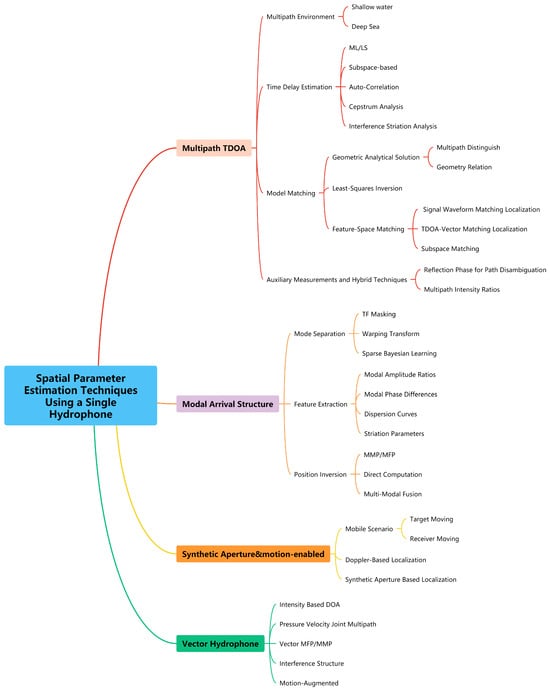
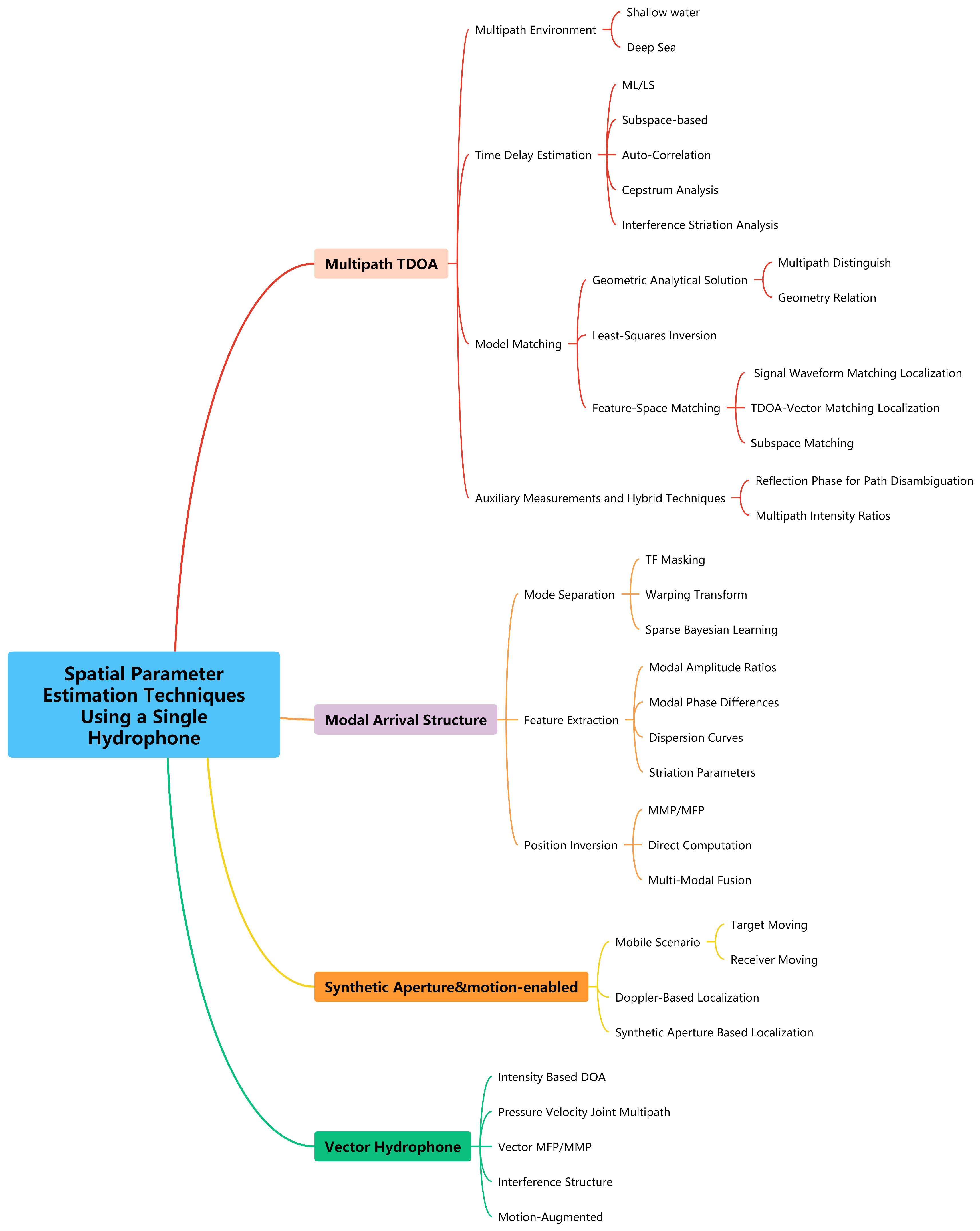
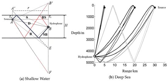
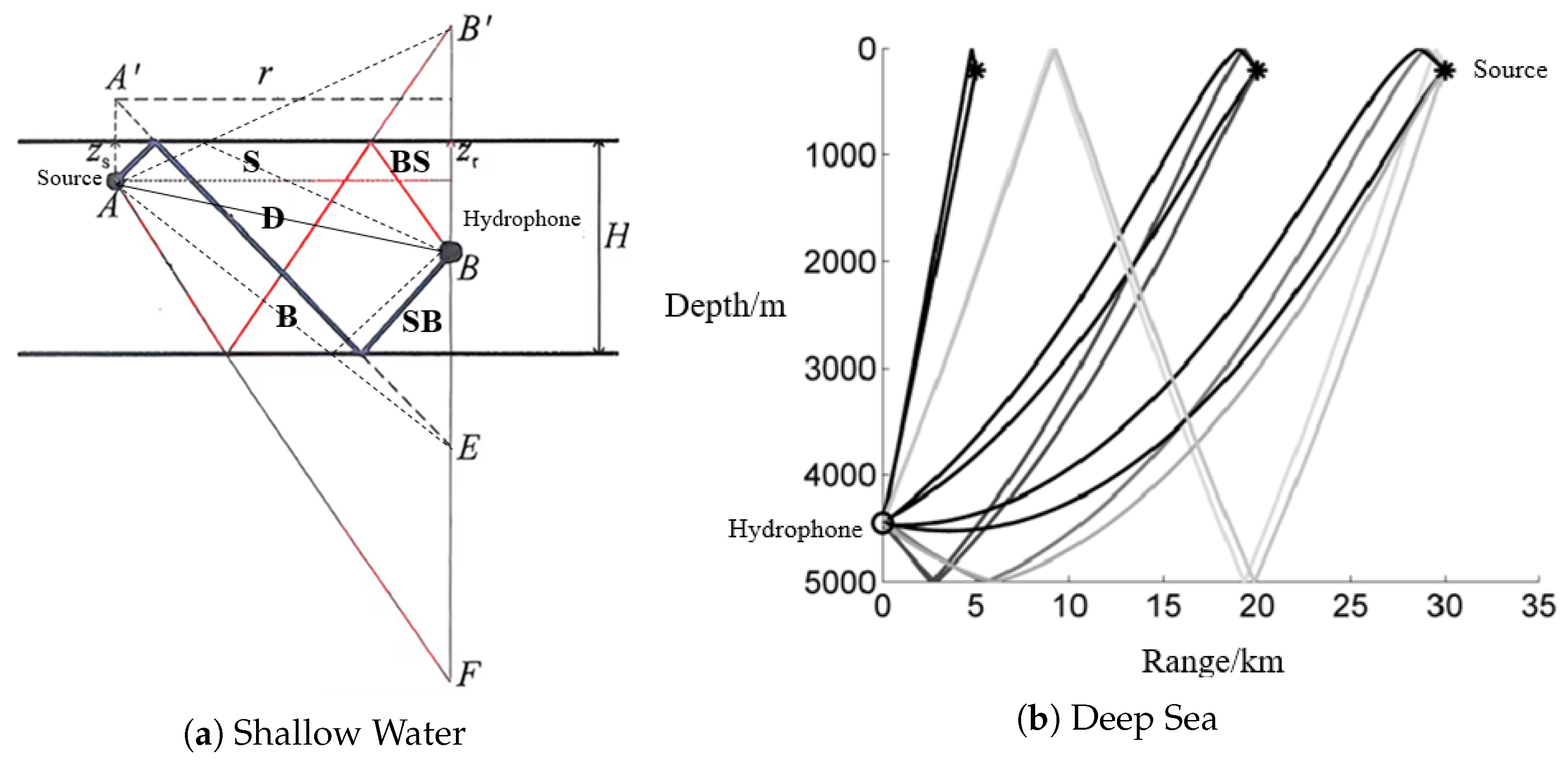
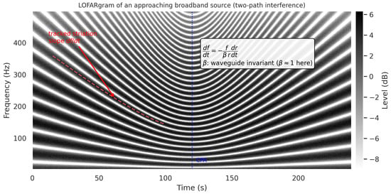
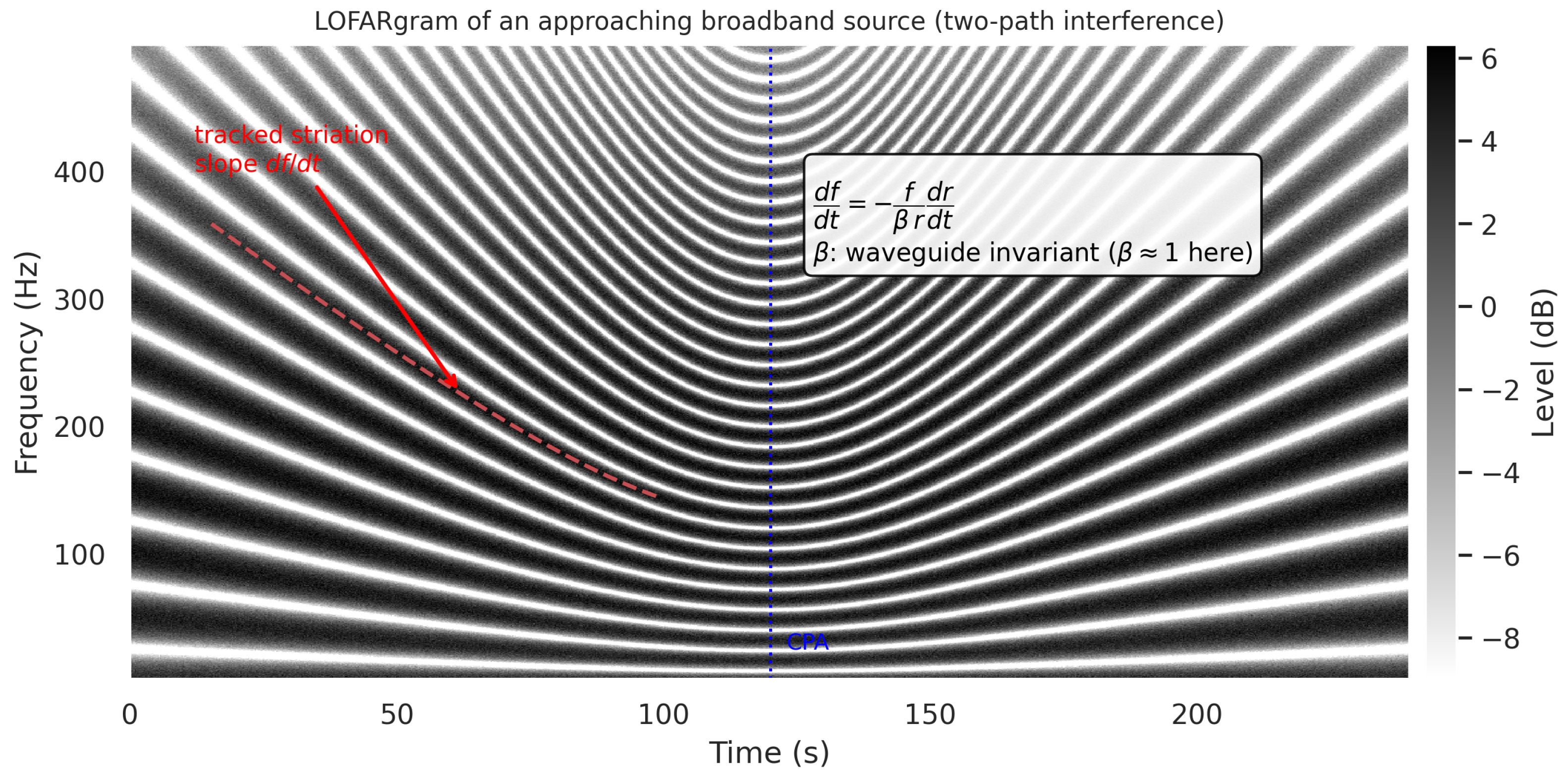
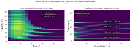
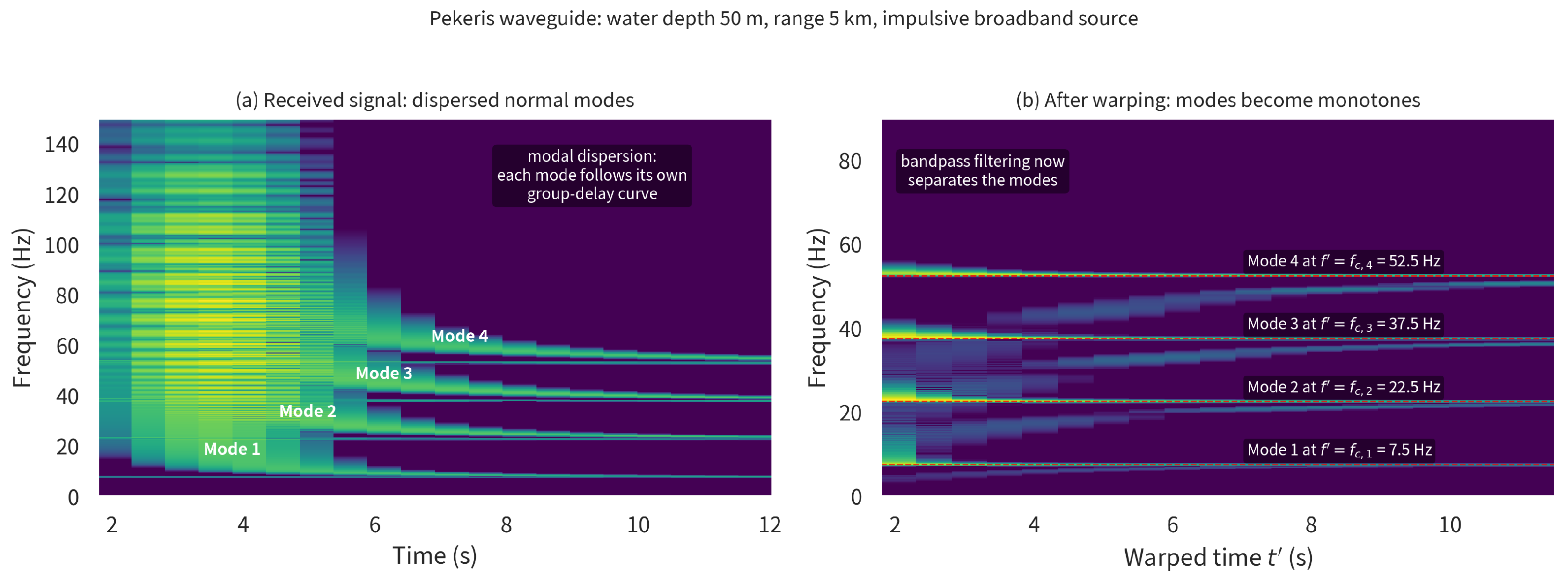
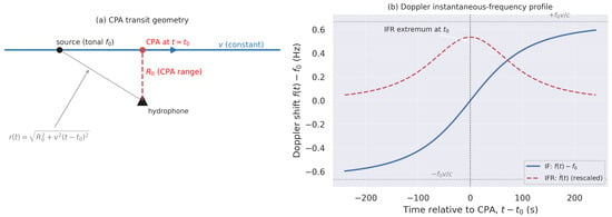
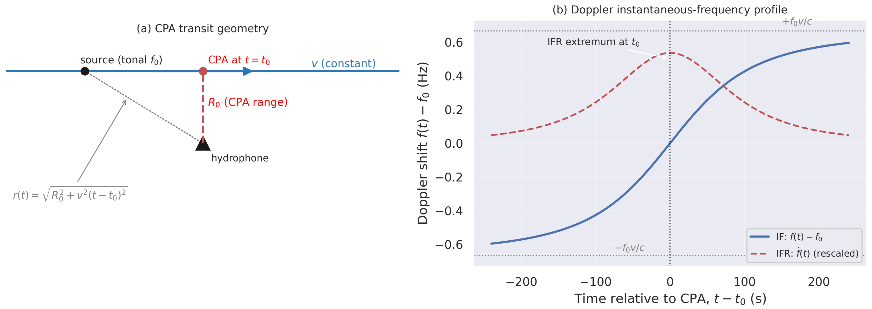
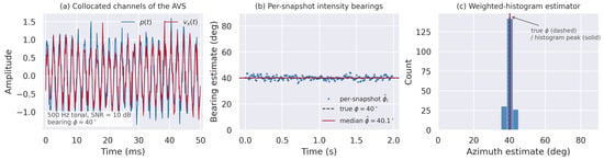
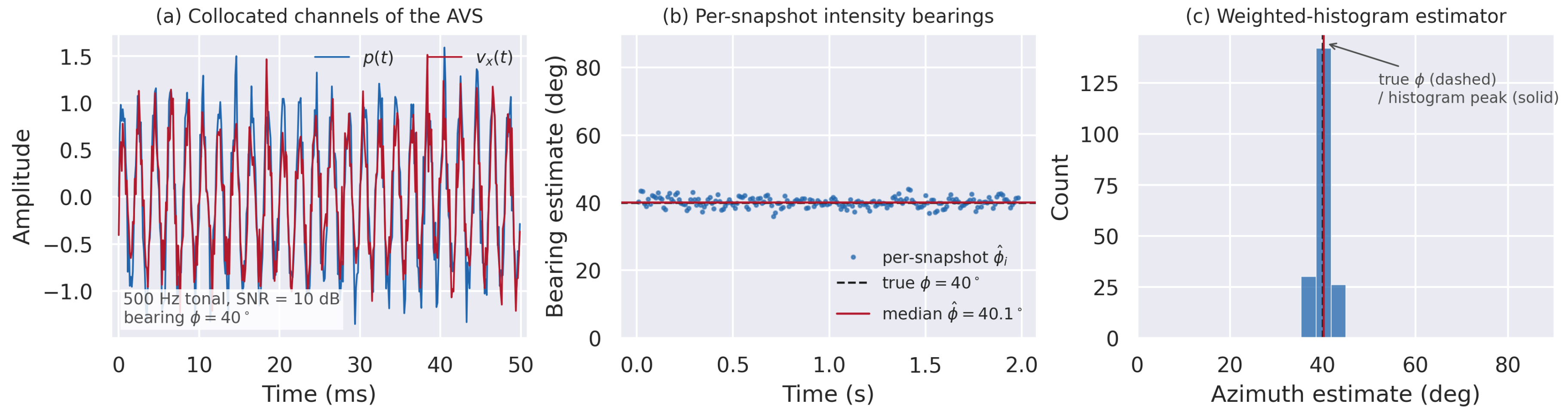
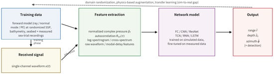
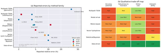
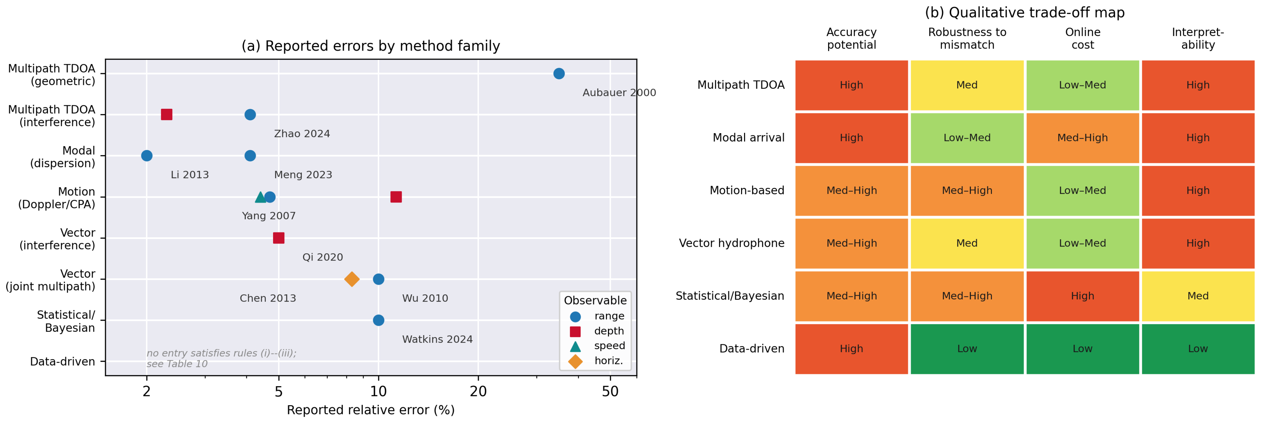

Disclaimer/Publisher’s Note: The statements, opinions and data contained in all publications are solely those of the individual author(s) and contributor(s) and not of MDPI and/or the editor(s). MDPI and/or the editor(s) disclaim responsibility for any injury to people or property resulting from any ideas, methods, instructions or products referred to in the content. |
© 2026 by the authors. Licensee MDPI, Basel, Switzerland. This article is an open access article distributed under the terms and conditions of the Creative Commons Attribution (CC BY) license.